Provable orbit recovery over SO(3) from the non-uniform second moment
We study the recovery of an unknown three-dimensional band-limited signal from multiple noisy observations that are randomly rotated by latent elements of SO(3), where the rotations are drawn from an unknown, non-uniform distribution. Because the rot…
Authors: Tamir Bendory, Dan Edidin, Josh Katz
PR O V ABLE ORBIT RECO VER Y O VER SO(3) FR OM THE NON-UNIF ORM SECOND MOMENT T AMIR BENDOR Y, D AN EDIDIN, JOSH KA TZ ∗ , SHA Y KREYMER, AND NIR SHAR ON Abstract. W e study the reco very of an unkno wn three-dimensional band-limited signal from multiple noisy observ ations that are randomly rotated by laten t elemen ts of SO(3), where the rotations are drawn from an unkno wn, non-uniform distribution. Because the rotations are unobserv ed, only the signal orbit under the rotation group can b e reco vered. W e sho w that the signal orbit and the rotation distribution are join tly identifiable from the first and second momen ts. This yields an impro ved high-noise sample complexit y that scales quadratically with the noise v ariance, rather than cubically as in the uniform-rotation case. W e further develop a prov able, computationally efficient reconstruction algorithm that re- co vers the 3-D signal b y successively solving a sequence of w ell-conditioned linear systems. The algorithm is v alidated through extensiv e n umerical exp erimen ts. Our results provide a principled and tractable framework for high-noise 3-D orbit recov ery , with p oten tial rele- v ance to cry o-electron microscopy and cry o-electron tomography mo deling, where molecules are observ ed in unknown orientations. 1. Introduction W e study the problem of reco v ering a 3-D signal from its randomly rotated and noisy observ ations. Sp ecifically , w e aim to estimate an unkno wn signal x ∈ V from n samples of the form (1) y i = g i · x + ε i , i = 1 , . . . , n, where g i are random elements dra wn from a distribution ρ on the rotation group SO(3), and ε i are i.i.d. Gaussian noise terms with zero mean and v ariance σ 2 . W e assume that V is a finite-dimensional space of band-limited functions on R 3 and that ρ is a non-uniform distribution ov er SO(3); precise mathematical mo dels are provided in the following sections. Our goal is to recov er x from the observ ations y 1 , . . . , y n , with the rotations g 1 , . . . , g n b eing unkno wn and the noise level σ p oten tially large. Imp ortan tly , since b oth the signal and the rotations are unknown, x is identifiable only up to a global rotation; that is, only its SO(3)-orbit can b e recov ered. The mo del (1) is a sp ecial case of a broader class of problems in which the goal is to estimate a signal from noisy samples sub ject to unknown group actions. This class is com monly known as orbit r e c overy problems or multi-r efer enc e alignment , e.g., [4, 8, 24]. When the noise level is lo w, a standard approach is to first estimate the laten t group elements from the samples, then align the observ ations accordingly , and finally av erage to reduce noise [33, 34, 25]. In high- noise regimes, how ev er, reliably estimating these group elements (e.g., rotations) b ecomes Date : F ebruary 25, 2026. ∗ Appro ved for Public Release; Distribution Unlimited. Public Release Case Number 26-0162. Affiliation with the MITRE Corp oration is for identification purp oses only and is not intended to con vey or imply MITRE’s concurrence with, or supp ort for, the p ositions, opinions, or viewp oin ts expressed b y the author. © 2026 The MITRE Corp oration. ALL RIGHTS RESER VED. 1 2 difficult, making alignment-based pro cedures unreliable [14]. In such settings, one typically turns to metho ds that estimate the signal directly while marginalizing o v er the unkno wn transformations; t w o p opular metho ds are the exp ectation-maximization algorithm and the metho d of moments [32, 17, 40, 31, 30]. This work fo cuses on the latter. Motiv ation: Electron-microscop y-based tec hnologies for structural biology . The primary motiv ation for studying orbit recov ery problems of the form (1) comes from single-particle cry o-electron microscopy (cryo-EM), the leading technology for determining the 3-D structure of biological macromolecules [23, 3]. In cry o-EM, one seeks to recov er a 3-D (band-limited) function representing the molecular densit y from man y noisy 2-D tomo- graphic pro jections. Eac h pro jection corresp onds to the molecule viewed after an unkno wn, randomly drawn 3-D rotation, so the observ ations are related through laten t group actions [7]. Mo del (1) captures the same cen tral statistical difficult y—estimating a signal from mul- tiple noisy , randomly rotated copies—while abstracting aw a y the additional complication in tro duced by the pro jection operator. In Section 5, we mak e this connection precise by relating (1) to the cry o-EM forw ard mo del and outlining ho w the metho ds developed here can b e p oten tially extended to incorp orate pro jections. Mo del (1) is also closely connected to cryo-electron tomograph y (cry o-ET), an emerging imaging mo dalit y for visualizing cellular architecture, including organelles and macromolec- ular assem blies [13, 28, 37]. In cry o-ET, a 3-D specimen (e.g., a cell) is imaged b y collecting a tilt series of 2-D pro jections at kno wn viewing angles. These pro jections are then integrated to pro duce a 3-D tomogram that preserves the in situ spatial arrangemen t of macromolecules within the cell. Researchers often extract smaller 3-D sub-volumes from the tomogram, called subtomograms, cen tered on macromolecules of interest. While real tomograms contain a het- erogeneous mixture of structures, it is useful to consider an idealized setting in which the v olume contains many instances of a single underlying structure x , eac h app earing in an un- kno wn, random orientation. Under this abstraction, the statistical structure aligns naturally with (1), whic h mo dels observ ations as noisy , randomly transformed copies of a common signal [39]. The metho d of momen ts and sample complexit y . A remark able line of w ork has rev ealed a close connection b et w een the metho d of momen ts and the information-theoretic limits of orbit reco v ery . In [2, 1, 4], it w as sho wn that, in the high-noise regime, the minimal n um b er of samples required for accurate signal estimation (i.e., the sample complexit y) scales as σ 2 d , where d is the smallest moment order that uniquely determines the signal’s orbit from the observ ations. F or instance, in mo del (1) with SO(3) transformations dra wn uniformly at random, one has d = 3, and consequen tly the sample complexity scales as σ 6 [10]. More generally , the σ 6 scaling also arises in many orbit recov ery mo dels under uniform group actions [8, 5, 4, 16]. Con tribution. Much of the existing w ork on orbit reco v ery problems fo cuses on identifia- bilit y: determining when a moment-matc hing form ulation, which t ypically inv olv es a system of p olynomial equations, admits a unique solution and its implication on sample complex- it y . In practice, how ev er, the field remains largely driven b y heuristic algorithms that lac k rigorous theoretical guaran tees; prominen t examples include [11, 29, 27, 41]. This paper mak es a significan t step forward b y in troducing a computationally efficien t algorithm for signal reco v ery from the second moment when the distribution of rotations is non-uniform, accompanied b y pro v able theoretical guaran tees. W e sho w that, in this setting, the unkno wn 3 signal and the rotation distribution are identifiable from the second momen t, which implies a sample complexity scaling as σ 4 . W e further develop a computationally efficient, prov able, and stable recov ery algorithm that reconstructs the 3-D function b y successiv ely solving a sequence of w ell-conditioned linear systems. This result complemen ts our previous work [10], whic h addressed recov ery under uniformly distributed rotations via the third momen t, and generalized [15] from SO(2) to SO(3). P ap er organization. The pap er is organized as follo ws. Section 2 reviews relev ant har- monic analysis on compact groups and form ulates the momen ts in represen tation-theoretic terms. Section 3 presen ts and prov es the main results on signal recov ery from the second momen t. Section 4 introduces the reco v ery algorithm—based on successively solving linear systems—and demonstrates its effectiveness n umerically , including empirical studies of ro- bustness to noise and the impact of the distribution. Finally , Section 5 outlines potential extensions of the approach to the cryo-EM problem. 2. Back gr ound 2.1. Harmonic analysis on compact groups. A function ρ ∈ L 2 ( G ) is determined by its F ourier c o efficients for each irreducible representation V of G. If φ : G → U ( V ) is a unitary represen tation of G , the F ourier co efficien t of V is the op erator on V defined by (2) ˆ ρ ( V ) = Z G ρ ( g ) φ V ( g ) ∗ dg , where dg is the Haar measure on G with total integral one, φ V ( g ) is the image of g in U ( V ), and φ V ( g i ) ∗ denotes the adjoin t. Let ˆ G b e the set of distinct irreducible represen tations of G . The function ρ is recov ered from its F ourier co efficien ts by the F ourier in version formula (3) ρ ( g ) = X V ∈ ˆ G (dim V ) T r( ˆ ρ ( V ) φ V ( g )) . In the case where ρ ( g ) dg defines a probability distribution, then the normalization condi- tion R G ρ ( g ) dg = 1 implies that ˆ ρ ( 1 ) = 1, where 1 denotes the trivial represen tation. The uniform distribution corresp onds to the case where ˆ ρ ( V ) is the 0-op erator for all non-trivial irreducible representations. By contrast, for a “generic” distribution, the F ourier co efficien ts ˆ ρ ( V ) are inv ertible op erators for all irreducibles V . 2.1.1. Harmonic analysis over SO(3) . Giv en our focus on the group SO(3), w e briefly review the spherical harmonics and Wigner D -matrices, which pro vide explicit bases for L 2 ( S 2 ) and L 2 (SO(3)), resp ectiv ely . The spherical harmonics Y m ℓ : S 2 → C for ℓ ≥ 0 and − ℓ ≤ m ≤ ℓ form an orthonormal basis for L 2 ( S 2 ). Using the Condon–Shortley phase conv en tion, they are defined as (4) Y m ℓ ( θ , φ ) = s 2 ℓ + 1 4 π ( ℓ − m )! ( ℓ + m )! P m ℓ (cos θ ) e imφ , where P m ℓ denotes the asso ciated Legendre p olynomial. F or each ℓ , the span (5) H ℓ = span { Y m ℓ : − ℓ ≤ m ≤ ℓ } 4 is an irreducible representation of SO(3) of dimension 2 ℓ + 1. The P eter-W eyl decomp osition giv es (6) L 2 ( S 2 ) = ∞ M ℓ =0 H ℓ . A signal in L 2 ( S 2 ) is L -band limited if it lies in the subspace ⊕ L ℓ =0 H ℓ . Throughout the pap er, w e consider band-limited signals and use the notation L 2 ( S 2 ) L to denote the subspace of L - band-limited signals in L 2 ( S 2 ). F or each ℓ , the representation π ℓ : SO(3) → U (2 ℓ + 1) acts on H ℓ b y rotation of functions. The matrix elements of π ℓ in the spherical harmonic basis are the Wigner D -functions : (7) D ℓ m,m ′ ( g ) = ⟨ Y m ℓ , g · Y m ′ ℓ ⟩ . Using the ZYZ Euler angle parameterization g = R z ( α ) R y ( β ) R z ( γ ) with α, γ ∈ [0 , 2 π ) and β ∈ [0 , π ], the Wigner D -functions factor as (8) D ℓ m,m ′ ( α, β , γ ) = e − imα d ℓ m,m ′ ( β ) e − im ′ γ , where d ℓ m,m ′ ( β ) is the Wigner small- d matrix, whic h can b e expressed in terms of Jacobi p oly- nomials. The normalized functions √ 2 ℓ + 1 D ℓ m,m ′ form an orthonormal basis for L 2 (SO(3)) with respect to the Haar measure. Consequen tly , any probability density ρ ∈ L 2 (SO(3)) admits the F ourier expansion (9) ρ ( g ) = ∞ X ℓ =0 (2 ℓ + 1) T r ˆ ρ ( H ℓ ) D ℓ ( g ) , where the F ourier co efficien t ˆ ρ ( H ℓ ) ∈ C (2 ℓ +1) × (2 ℓ +1) is defined by (10) ˆ ρ ( H ℓ ) m,m ′ = Z SO(3) ρ ( g ) D ℓ m,m ′ ( g ) dg . Throughout the text, w e use the notations ˆ ρ ℓ m [ m ′ ] and ˆ ρ ( H ℓ ) m,m ′ in terc hangeably to represent the co efficien ts that represen t the distribution. 2.1.2. Clebsch-Gor dan c o efficients. The tensor pro duct of tw o irreducible representations decomp oses as (11) H ℓ 1 ⊗ H ℓ 2 ∼ = ℓ 1 + ℓ 2 M k = | ℓ 1 − ℓ 2 | H k . The Clebsch-Gordan (CG) co efficien ts ⟨ ℓ 1 m 1 ℓ 2 m 2 | ℓ 3 m 3 ⟩ provide the explicit intert win- ing maps. They satisfy the selection rule m 1 + m 2 = m 3 and v anish unless | ℓ 1 − ℓ 2 | ≤ ℓ 3 ≤ ℓ 1 + ℓ 2 . These co efficien ts are cen tral to our second momen t formulas, as they gov ern the 5 pro jection H ℓ 2 ⊗ H ℓ 3 → H ℓ 1 , and they are explicitly given by ⟨ ℓ 1 m 1 ℓ 2 m 2 | ℓ m ⟩ = δ m,m 1 + m 2 s (2 ℓ + 1)( ℓ + ℓ 1 − ℓ 2 )!( ℓ − ℓ 1 + ℓ 2 )!( ℓ 1 + ℓ 2 − ℓ )! ( ℓ 1 + ℓ 2 + ℓ + 1)! × p ( ℓ + m )!( ℓ − m )!( ℓ 1 − m 1 )!( ℓ 1 + m 1 )!( ℓ 2 − m 2 )!( ℓ 2 + m 2 )! × X k ( − 1) k k !( ℓ 1 + ℓ 2 − ℓ − k )!( ℓ 1 − m 1 − k )!( ℓ 2 + m 2 − k )!( ℓ − ℓ 2 + m 1 + k )!( ℓ − ℓ 1 − m 2 + k )! . (12) The following lemma gives the explicit relationship b et w een the pro jection op erators and the Clebsc h-Gordan co efficien ts [12]. Lemma 2.1. F or a given ℓ , let a ℓ = ( a ℓ − ℓ , . . . , a ℓ ℓ ) ∈ H ℓ denote a ve ctor exp ande d in the spheric al harmonic b asis. F or | ℓ 2 − ℓ 3 | ≤ ℓ 1 ≤ ℓ 2 + ℓ 3 , the pr oje ction ( a ℓ 2 ⊗ a ℓ 3 ) ℓ 1 ∈ H ℓ 1 has c omp onents with r esp e ct to the spheric al harmonic b asis of H ℓ 1 ( a ℓ 2 ⊗ a ℓ 3 ) ℓ 1 k 1 = X k 2 ,k 3 k 2 + k 3 = k 1 ⟨ ℓ 2 k 2 ℓ 3 k 3 | ℓ 1 k 1 ⟩ a ℓ 2 k 2 a ℓ 3 k 3 , wher e − ℓ 1 ≤ k 1 ≤ ℓ 1 and the sum is over | k 2 | ≤ ℓ 2 and | k 3 | ≤ ℓ 3 . 2.1.3. In-plane uniform distributions. Next, w e introduce and study in-plane-uniform distri- butions. As will b e explained in Section 3, these distributions play a key role in cry o-EM. A probabilit y distribution ρ ∈ L 2 (SO(3)) is in-plane uniform if ρ ( g h ) = ρ ( g ) for all h ∈ SO(2), where SO(2) is embedded as rotations ab out the z -axis; i.e., matrices of the form cos θ sin θ 0 − sin θ cos θ 0 0 0 1 , θ ∈ [0 , 2 π ) . Suc h distributions correspond to viewing directions that are uniformly distributed in the in-plane angle but may hav e an arbitrary tilt distribution. Note that if ρ is in-plane uni- form, then g · ρ is as well, where g · ρ ∈ L 2 (SO(3)) is the function defined b y the formula ( g · ρ )( g ′ ) = ρ ( g − 1 g ′ ) for all g ′ ∈ G . In particular, an in-plane uniform distribution is a function L 2 (SO(3)) SO(2) , where SO(2) acts on ρ ∈ L 2 (SO(3)) b y ( hρ )( g ) = ρ ( g h ). Since this action commutes with the usual G action on L 2 (SO(3)), L 2 (SO(3)) SO(2) is an SO(3) sub- represen tation. The following lemma sho ws that, viewed as a function on SO(3), elements of L 2 (SO(3)) SO(2) can b e characterized in terms of their F ourier co efficien ts with resp ect to the bases of spherical harmonics for eac h irreducible representation H ℓ of SO(3). Lemma 2.2. With r esp e ct to the b asis { Y ℓ m } − ℓ ≤ m ≤ ℓ of spheric al harmonics for H ℓ , the F ourier c o efficients of a function ρ ∈ L 2 (SO(3)) SO(2) satisfy (13) ˆ ρ ℓ m [ m ′ ] = 0 unless m ′ = 0 . That is, only the m ′ = 0 c olumn of e ach F ourier c o efficient matrix is non-zer o. 6 Pr o of. Since ρ is H -in v ariant, we hav e that ˆ ρ ℓ m [ m ′ ] = Z SO(3) ρ ( g ) D ℓ m,m ′ ( g ) dg = Z SO(3) ρ ( g h ) D ℓ m,m ′ ( g ) dg = Z SO(3) ρ ( g ) D ℓ m,m ′ ( g h ) dg , where the second equalit y follows from a change of v ariables g 7→ g h . No w, D ℓ m,m ′ ( g ) = ⟨ Y m ℓ , g · Y m ′ ℓ ⟩ , and if h ∈ SO(2) corresp onds to rotation by an angle θ ab out the z -axis, D ℓ m,m ′ ( g h ) = ⟨ Y m ℓ , ( g h ) · Y m ′ ℓ ⟩ = ⟨ Y m ℓ , g · ( h · Y m ′ ℓ ) ⟩ = e ιm ′ θ ⟨ Y m ℓ , g · Y m ′ ℓ ⟩ = e ιm ′ θ D ℓ m,m ′ ( g ) , since the action of SO(2) is diagonalized with resp ect to the spherical harmonic basis. Hence, w e hav e that ˆ ρ ℓ m [ m ′ ] = e ιm ′ θ ˆ ρ ℓ m [ m ′ ] for all θ ∈ [0 , 2 π ), so if m ′ = 0 these co efficien ts v anish. □ Lemma 2.2 establishes that the space of SO(2)-inv arian t functions is isomorphic to L 2 ( S 2 ) via the isomorphism SO(3) / SO(2) ∼ = S 2 . 2.2. Signal and distribution models. W e mo del the target signal x as a real-v alued, radially discretized band-limited function supported at R spherical shells within the unit ball in R 3 . Expanded in spherical harmonics our function can b e represented as: (14) x ( r , θ , φ ) = L X ℓ =0 ℓ X m = − ℓ x ℓ m [ r ] Y m ℓ ( θ , φ ) , where r = 1 , . . . , R is a discrete parameter and θ , φ are spherical co ordinates. As such, our signal space can b e iden tified with the SO(3)-representation (15) V L = L M ℓ =0 H R ℓ . Giv en a bandlimit of L on the signal and a distribution ρ ∈ L 2 (SO(3)), the corresp onding bandlimited distribution ρ L is the function obtained by expanding the distribution ρ up to band L . It can b e expressed in the basis of D -Wigner matrices as follows: (16) ρ L ( g ) = L X ℓ =0 ℓ X m = − ℓ ℓ X m ′ = − ℓ ˆ ρ ℓ m [ m ′ ] D ℓ m,m ′ ( g ) , g ∈ SO(3) . 2.3. A F ourier-theoretic p ersp ectiv e of SO(3) momen ts. Here, we consider the first t w o p opulation momen ts M 1 ( ρ, x ) : = Z G ρ ( g )( g x ) dg , (17) M 2 ( ρ, x ) : = Z G ρ ( g )( g x ) ⊗ 2 dg . (18) 7 W e represent x ∈ V L = L L ℓ =0 H R ℓ as an ( L + 1)-tuple of signal matric es x = ( X 0 , . . . , X L ) , where X ℓ is a (2 ℓ + 1) × R matrix of spherical harmonic co efficien ts X ℓ = ( x ℓ m [ r ]) for m = − ℓ, . . . , ℓ and r = 1 , . . . , R . First momen t. The first non-uniform p opulation moment is an elemen t of V whic h is represen ted by the ( L + 1)-tuple of matrices (19) M 1 ( ρ, x ) = ( ˆ ρ ( H 0 ) ∗ X 0 , . . . , ˆ ρ ( H L ) ∗ X L ) . Hence, if w e know the first momen t, w e know each of the matrices ˆ ρ ( H ℓ ) ∗ X ℓ . In terms of the Wigner and spherical harmonic bases, the ( m ′ , s ) en try of ˆ ρ ( H ℓ ) ∗ X ℓ is: (20) ( ˆ ρ ( H ℓ ) ∗ X ℓ ) ( m ′ ,s ) = ℓ X m = − ℓ ˆ ρ ℓ m [ m ′ ] x ℓ m [ s ] . Note that, because ρ is a probability distribution, R G ρ ( g ) dg = 1, so X 0 is alwa ys known from the first moment. Second momen t. The tensor V ⊗ V decomp oses as a sum of tensor pro ducts H R i ⊗ H R j . In turn, w e can view H R i ⊗ H R j as a sum of R 2 summands all equal to H i ⊗ H j . The summand H i ⊗ H j decomp oses into irreducibles as (21) ( H i ⊗ H j ) = i + j M ℓ = | i − j | H ℓ . Th us, the tensor X i ⊗ X j decomp oses in to comp onen ts ( X i ⊗ X j ) ℓ , whic h live in ( H ℓ ) R 2 . View ed this wa y , the second momen t of x ∈ V , whic h is an elemen t of V ⊗ V , decomp oses as a sum (22) M 2 ( ρ, x ) = X i,j i + j X ℓ = | i − j | ˆ ρ ( H ℓ ) ∗ ( X i ⊗ X j ) ℓ , where the inner sum reflects the decomp osition of H R i ⊗ H R j in to its isot ypical pieces follo wing the decomp osition (21). In particular, if we know the second moment we know eac h of the summands ˆ ρ ( H ℓ ) ∗ ( X i ⊗ X j ) ℓ in the decomp osition (22). W e will denote by M 2 ( x ; H i , H j , H k ) the summand ˆ ρ ( H k ) ∗ ( X i ⊗ X j ) k . The columns of the matrices X i are the vectors x i [ s ] ∈ H i for s = 1 , . . . , R . Thus, the tensor X i ⊗ X j can b e viewed as a collection of R 2 tensors x i [ s 1 ] ⊗ x j [ s 2 ] ∈ H i ⊗ H j for 1 ≤ s 1 , s 2 ≤ R . Applying Lemma 2.1 to the second momen t (22), we obtain an explicit formula in terms of Clebsc h-Gordan co efficien ts for the action of the op erator ˆ ρ ( H ℓ ) ∗ on ( x i [ s 1 ] ⊗ x j [ s 2 ]) ℓ . T o mak e this precise, we c hange notation slightly and fix bands ℓ 1 , ℓ 2 , ℓ 3 satisfying the triangle inequalit y and shell indices s 2 , s 3 ∈ { 1 , . . . , R } . Then, for − ℓ 1 ≤ m ≤ ℓ 1 , the m -th en try in the v ector ˆ ρ ( H ℓ 1 ) ∗ ( x ℓ 2 [ s 2 ] ⊗ x ℓ 3 [ s 3 ]) ℓ 1 is M 2 ( ρ, x ; H ℓ 1 [ m ] , H ℓ 2 [ s 2 ] , H ℓ 3 [ s 3 ]) : = X k 2 + k 3 = k 1 | k i |≤ ℓ i ⟨ ℓ 2 k 2 ℓ 3 k 3 | ℓ 1 k 1 ⟩ ˆ ρ ℓ 1 k 1 [ m ] x ℓ 2 k 2 [ s 2 ] x ℓ 3 k 3 [ s 3 ] . (23) 8 3. Main resul ts W e b egin this section by explicitly introducing the signal and distribution mo dels. These mo dels will also serve us in the n umerical exp erimen ts in Section 4. Then, we state the t w o main theorems on signal reco v ery from the second momen t for a generic distribution on SO(3) (Theorem 3.1) and one for a generic in-plane uniform distribution on SO(3) (Theorem 3.2). The results are then prov ed in Section 3.2 and Section 3.3. 3.1. Main results. W e are no w ready to present the main theoretical results of this pap er. Theorem 3.1. L et ρ ∈ L 2 (SO(3)) b e a distribution whose F ourier c o efficients ˆ ρ ( H ℓ ) ar e invertible for 0 ≤ ℓ ≤ L . Then, if R ≥ 3 , and x ∈ V L is a generic signal, then the p air ( ρ L , x ) is determine d, up to a glob al r otation, by the first and se c ond moments M 1 ( ρ, x ) and M 2 ( ρ, x ) . By generic signal we mean that there is a non-empt y Zariski op en subset of V L suc h that the conclusion of the theorem holds. Note that this set may dep end on the distribution ρ . While Theorem 3.1 assumes that the F ourier co efficien ts of the distribution are in v ertible (at least up to band L ), this assumption may not b e exp erimen tally justified. In particular, in cry o-EM the distribution of in-plane rotations is uniform, since eac h in-plane rotation is equally lik ely to o ccur [7]. The follo wing theorem sho ws that in this imp ortan t scenario— where the in-plane rotation distribution is uniform but otherwise generic—the theory con- tin ues to hold, with only a mo dest increase in the required num ber of shells. Theorem 3.2. L et ρ b e an in-plane uniform distribution whose non-vanishing F ourier c o ef- ficients { ˆ ρ ℓ m [0] } with 0 ≤ ℓ ≤ L ar e generic. If R ≥ 4 , then, for a generic signal x ∈ V L , the p air ( ρ L , x ) is determine d, up to a glob al r otation, by the first and se c ond moments M 1 ( ρ, x ) and M 2 ( ρ, x ) . By generic F ourier co efficien ts and generic signal w e mean the follo wing. If we let U L denote the space of all p ossible { ˆ ρ ℓ m [0] } with 0 ≤ ℓ ≤ L , then there is a Zariski op en set in U L suc h that the following holds: F or every in-plane uniform distribution ρ whose non- v anishing F ourier coefficients lie in this Zariski op en set, there is a corresp onding Zariski op en set in the signal space V L suc h that for x in this op en set the conclusion of the theorem holds. Corollary 3.3. Consider the class of distributions and signals define d in The or ems 3.1 and 3.2. In the high-noise r e gime, wher e n, σ → ∞ , the sample c omplexity r e quir e d to estimate a signal fr om observations of (1) sc ales as n = ω ( σ 4 ) . Remark 3.4 (The optimality of the results) . It is unclear whether the results of Theorem 3.1 and Theorem 3.2 are optimal. In particular, the b ounds of R = 3 and R = 4 may b e an artifact of the pro of tec hnique of the sp ecific algorithm we analyze. 3.2. Pro of of Theorem 3.1. Our pro of of Theorem 3.1 is inductive and constructiv e. F or eac h ℓ , we first use the second moment to solve for the generalized F ourier co efficien t ˆ ρ ( H ℓ ), assuming that F ourier co efficien ts ˆ ρ ( H j ) and signal co efficien ts X j are known for j ≤ l . Ha ving done this, w e can easily determine the signal co efficien t matrix X ℓ from the first momen t b ecause the first moment yields ˆ ρ ( H ℓ ) ∗ X ℓ . Hence, if ˆ ρ ( H ℓ ) is inv ertible w e can determine X ℓ as w ell. This alternating pro cedure is illustrated in Figure 1. 9 Signal Distribution X 0 ˆ ρ ( H 0 ) X 1 ˆ ρ ( H 1 ) ˆ ρ ( H 2 ) X 2 ˆ ρ ( H 3 ) X 3 ˆ ρ ( H 4 ) X 4 . . . . . . 1 2 3 4 5 6 7 kno wn (base case) kno wn Figure 1. A sc hematic illustration of the frequency-marching reco v ery . Sig- nal co efficien ts (blue, left) and distribution F ourier co efficien ts (orange, right) are recov ered at progressively higher frequency bands. A t each band ℓ ≥ 2, the distribution ˆ ρ ( H ℓ ) is first solved from the second moment using previously reco v ered signal co efficien ts (diagonal and dashed arrows), and then X ℓ is re- co v ered from the first momen t by inv erting ˆ ρ ( H ℓ ) (horizontal arrows). The n um b ers show the order of computation. Base case. W e b egin by recalling that for any compact group, the G -in v arian t part of the d - th momen t with resp ect to an arbitrary probabilit y distribution is the uniform d -th moment. In particular, the uniform second moment is known from the non-uniform second moment, so b y [9] w e kno w the matrices X ∗ ℓ X ℓ for eac h ℓ . Moreov er, w e kno w X 0 since w e know ˆ ρ ( 1 ) = 1 for an y probability distribution and w e know ˆ ρ ( 1 ) X 0 . Let X ′ 1 b e an y square ro ot of the Gram matrix X ∗ 1 X 1 . Once we fix X ′ 1 , we can uniquely determine the F ourier co efficien t ˆ ρ ( H 1 ) from the first moment ˆ ρ ( H 1 ) ∗ X ′ 1 since we assume that we ha v e at least three shells ( R ≥ 3) and the latter implies that the rank of X ′ 1 is three for a generic signal. Hence, w e ha ve reco vered the first bands of b oth the distribution and signal up to the same O(3) action, which is equiv alent to reco v ering their joint SO(3) orbit up to a global sign. W e can eliminate the sign ambiguit y by comparing ( ˆ ρ ( H 1 ) ′ ) ∗ ( X ′ 1 ⊗ X ′ 1 ) 1 with the comp onen t ˆ ρ ( H 1 ) ∗ ( X 1 ⊗ X 1 ) 1 of the second moment. Induction step. Now, supp ose that w e ha ve determined the following F ourier co efficien ts, ˆ ρ ( 1 ) , . . . , ˆ ρ ( H ℓ − 1 ), and thus the corresp onding signal matrices X 1 , . . . , X ℓ − 1 . W e will sho w that w e can solve a linear system to determine the F ourier co efficien t ˆ ρ ( H ℓ ). 10 Lemma 3.5. Supp ose the orbit of ( ρ, x ) ∈ L 2 (SO(3)) ℓ − 1 × ( L 2 ( S 2 ) ℓ − 1 ) R is fixe d with ℓ > 1 . If − ℓ ≤ s ≤ ℓ , the distribution c o efficients ρ ℓ k [ s ] for − ℓ ≤ k ≤ ℓ ar e determine d by the invariants M 2 ( ρ, x ; H ℓ [ s 1 ] , H i [ s 2 ] , H ℓ − i [ s 3 ]) for 0 ≤ i ≤ ⌊ ℓ/ 2 ⌋ , pr ovide d that R ≥ 3 . Pr o of. F or fixed s 1 , the second moment equation (23) M 2 ( ρ, x ; H ℓ [ s 1 ] , H i [ s 2 ] , H ℓ − i [ s 3 ]) = X k 2 + k 3 = k 1 | k 1 |≤ ℓ, | k 2 |≤ i, | k 3 |≤ ℓ − i ⟨ i k 2 ( ℓ − i ) k 3 | ℓ k 1 ⟩ ˆ ρ ℓ k 1 [ s 1 ] x i k 2 [ s 2 ] x ℓ − i k 3 [ s 3 ] , giv es a linear equation in the 2 ℓ + 1 unkno wns ˆ ρ ℓ k [ s 1 ] with − ℓ ≤ k ≤ ℓ . The coefficients C ( x i [ s 2 ] , x ℓ − i [ s 3 ]) k = P k 1 − k 2 = k ⟨ i k 1 ( ℓ − i ) k 2 | ℓ k ⟩ x i [ s 2 ] k 1 x ℓ − i [ s 3 ] k 2 are bilinear forms in the v ariables x i,ℓ − i s,t [ s 2 , s 3 ] : = x i s [ s 2 ] x ℓ − i t [ s 3 ]. T aking indices ( s 2 , s 3 ) ∈ S i,ℓ − i [ R ], where S i,ℓ − i [ R ] = ( { (1 , 1) , . . . , (1 , R ) , (2 , 1) , . . . , ( R , 1) } if i = ℓ − i, { (1 , 1) , . . . , (1 , R ) } if i = ℓ − i, and v arying i from 0 to ⌊ ℓ/ 2 ⌋ , w e obtain ( ⌊ ℓ/ 2 ⌋ + 1) · (2 R − 1) equations. F or R ≥ 3, this giv es at least ( ⌊ ℓ/ 2 ⌋ + 1) · 5 ≥ 2 ℓ + 1 when ℓ ≥ 1. F or tw o distinct pairs ( s ′ 2 , s ′ 3 ) , ( s ′′ 2 , s ′′ 3 ) ∈ S i,ℓ − i [ R ], there are no algebraic relations b et w een the corresp onding sets of monomials, so w e ma y treat them as distinct sets of v ariables. Using the shorthand C ( { x i,ℓ − i s,t [ s 2 , s 3 ] } ) k for the co efficien t C ( x i [ s 2 ] , x ℓ − i [ s 3 ]) k , the co efficien t matrix is (24) M = C ( { x 0 ,ℓ s,t [1 , 1] } ) − ℓ · · · C ( { x 0 ,ℓ s,t [1 , 1] } ) ℓ . . . . . . C ( { x 0 ,ℓ s,t [1 , R ] } ) − ℓ · · · C ( { x 0 ,ℓ s,t [1 , R ] } ) ℓ C ( { x 0 ,ℓ s,t [2 , 1] } ) − ℓ · · · C ( { x 0 ,ℓ s,t [2 , 1] } ) ℓ . . . . . . C ( { x 0 ,ℓ s,t [ R, 1] } ) − ℓ · · · C ( { x 0 ,ℓ s,t [ R, 1] } ) ℓ C ( { x 1 ,ℓ − 1 s,t [1 , 1] } ) − ℓ · · · C ( { x 1 ,ℓ − 1 s,t [1 , 1] } ) ℓ . . . . . . C ( { x 1 ,ℓ − 1 s,t [1 , R ] } ) − ℓ · · · C ( { x 1 ,ℓ − 1 s,t [1 , R ] } ) ℓ C ( { x 1 ,ℓ − 1 s,t [2 , 1] } ) − ℓ · · · C ( { x 1 ,ℓ − 1 s,t [2 , 1] } ) ℓ . . . . . . C ( { x 1 ,ℓ − 1 s,t [ R, 1] } ) − ℓ · · · C ( { x 1 ,ℓ − 1 s,t [ R, 1] } ) ℓ . . . . . . C ( { x ⌊ ℓ/ 2 ⌋ , ⌈ ℓ/ 2 ⌉ s,t [1 , 1] } ) − ℓ · · · C ( { x ⌊ ℓ/ 2 ⌋ , ⌈ ℓ/ 2 ⌉ s,t [1 , 1] } ) ℓ . . . . . . C ( { x ⌊ ℓ/ 2 ⌋ , ⌈ ℓ/ 2 ⌉ s,t [1 , R ] } ) − ℓ · · · C ( { x ⌊ ℓ/ 2 ⌋ , ⌈ ℓ/ 2 ⌉ s,t [1 , R ] } ) ℓ C ( { x ⌊ ℓ/ 2 ⌋ , ⌈ ℓ/ 2 ⌉ s,t [2 , 1] } ) − ℓ · · · C ( { x ⌊ ℓ/ 2 ⌋ , ⌈ ℓ/ 2 ⌉ s,t [2 , 1] } ) ℓ . . . . . . C ( { x ⌊ ℓ/ 2 ⌋ , ⌈ ℓ/ 2 ⌉ s,t [ R, 1] } ) − ℓ · · · C ( { x ⌊ ℓ/ 2 ⌋ , ⌈ ℓ/ 2 ⌉ s,t [ R, 1] } ) ℓ . Since the forms C ( { x i,ℓ − i s,t [ s 2 , s 3 ] } ) k for k = − ℓ, . . . , ℓ are linearly indep enden t for each fixed ( s 1 , s 2 ), the matrix M has full rank o v er the field of rational functions. Th us, for generic 11 ( ρ, x ), the matrix has rank 2 ℓ + 1. In particular, the system has a unique solution for the en tries of the F ourier co efficien t matrix ˆ ρ ( H ℓ ). This completes the pro of of Lemma 3.5 and with it Theorem 3.1. □ 3.3. Pro of of Theorem 3.2. The pro of of Theorem 3.2 has a similar structure to the pro of of Theorem 3.1. How ev er, because the F ourier co efficien ts of an in-plane uniform distribution all ha v e rank one, we cannot use the first moment to solv e for the unkno wn matrices X ℓ if w e already know the F ourier co efficien t ˆ ρ ( H ℓ ). Because ˆ ρ ℓ m [ m ′ ] = 0 if m ′ = 0, the only non-zero terms in the second moment hav e the form M 2 ( ρ, x ; H i [0] , H j [ s 2 ] , H k [ s 3 ]) , for v arying v alues of i, j, k ∈ [0 , L ] and s 2 , s 3 ∈ [1 , R ]. Base case. The base case is essen tially the same as in the pro of Theorem 3.1. Because we ha v e at least three shells, w e may assume that the matrix X 1 has rank at least three and can therefore solve for the three non-zero en tries in ˆ ρ ( H 1 ) from the first moment ˆ ρ ( H 1 ) X 1 . Induction step. Let ℓ > 1 and supp ose all terms of the distribution and signal hav e b een determined up to band ℓ − 1, i.e., { ˆ ρ i k [0] } and { x i k [ s ] } are fixed for 1 ≤ i ≤ ℓ − 1, − i ≤ k ≤ i and 1 ≤ s ≤ R . Step 1: The case ℓ = 2 . Let ˆ ρ ( H 1 ) ∈ R 3 × 3 and X 1 ∈ R 3 × R b e fixed. W e first solv e for the distribution term, ˆ ρ ( H 2 ). W e use the equations { M 2 ( H 2 [0] , H 1 [ s 2 ] , H 1 [ s 3 ]) } with indices taking v alues in 1 ≤ s 2 ≤ R , s 3 = 1 and s 2 = 1, 2 ≤ s 3 ≤ R . This yields 2 R − 1 equations, whic h is at least dim( H 2 ) = 5 when R ≥ 3. No w w e solv e for the signal comp onen t X 2 . F or fixed 1 ≤ s 3 ≤ R , the R equations { M 2 ( ρ, x ; H 1 [0] , H 1 [ s 2 ] , H 2 [ s 3 ]) } with 1 ≤ s 2 ≤ R and the equation { M 2 ( ρ, x ; H 2 [0] , H 1 [1] , H 2 [ s 3 ]) } in v olve algebraically indep enden t co efficien ts. Therefore, we obtain R + 1 ≥ dim( H 2 ) = 5 (when R ≥ 4) indep enden t equations, which allows us to solve for x 2 [ s 3 ]. Step 2: The case ℓ > 2 . Fix 1 ≤ s 3 ≤ R . W e solv e for the 2 ℓ + 1 unknowns { x ℓ k [ s 3 ] } ℓ k = − ℓ using in v arian ts of the form M 2 ( H i [0] , H ℓ − i [ s 2 ] , H ℓ [ s 3 ]) for 1 ≤ i ≤ ℓ − 1 and 1 ≤ s 2 ≤ R . F or fixed i and s 2 , the second moment equation (23) M 2 ( ρ, x ; H i [0] , H ℓ − i [ s 2 ] , H ℓ [ s 3 ]) = X k 2 + k 3 = k 1 | k 1 |≤ i, | k 2 |≤ ( ℓ − i ) , | k 3 |≤ i ⟨ ( ℓ − i ) k 2 ℓ k 3 | i k 1 ⟩ ˆ ρ i k 1 [0] x ℓ − i k 2 [ s 2 ] x ℓ k 3 [ s 3 ] . giv es a linear equation in the unkno wns x ℓ k [ s 3 ], with co efficien ts C ( ˆ ρ i [0] , x ℓ − i [ s 2 ]) k = X k 1 − k 2 = k ⟨ ( ℓ − i ) k 1 ℓ k | i k 1 ⟩ ˆ ρ i k 1 [0] x ℓ − i k 2 [ s 2 ] that are bilinear forms in the v ariables y i,ℓ − i s,t [ s 2 ] : = ˆ ρ i s [0] x ℓ − i t [ s 2 ]. Let S [ R ] = { ( i, s 2 ) : 1 ≤ i ≤ ℓ − 1 , 1 ≤ s 2 ≤ R } ⊂ [1 , ℓ − 1] × [1 , R ] . T aking ( i, s 2 ) ∈ S [ R ] yields | S [ R ] | = ( ℓ − 1) · R linear equations. F or distinct pairs ( i, s 2 ) , ( i ′ , s ′ 2 ) ∈ S [ R ], there are no algebraic relations b et w een the corresp onding sets of monomials { y i,ℓ − i s,t [ s 2 ] } s,t and { y i ′ ,ℓ − i ′ s,t [ s ′ 2 ] } s,t : if i = i ′ the v ariables lie in different bands, and 12 if i = i ′ but s 2 = s ′ 2 the v ariables lie in differen t shells. Thus, w e ma y treat them as distinct sets of v ariables. Using the shorthand C ( { y i,ℓ − i s,t [ s 2 ] } ) k for the co efficien t C ( ˆ ρ i [0] , x ℓ − i [ s 2 ]) k the co efficien t matrix is (25) M = C ( { y 1 ,ℓ − 1 s,t [1] } ) − ℓ · · · C ( { y 1 ,ℓ − 1 s,t [1] } ) ℓ . . . . . . C ( { y 1 ,ℓ − 1 s,t [ R ] } ) − ℓ · · · C ( { y 1 ,L − 1 s,t [ R ] } ) ℓ C ( { y 2 ,L − 2 s,t [1] } ) − ℓ · · · C ( { y 2 ,L − 2 s,t [1] } ) ℓ . . . . . . C ( { y L − 1 , 1 s,t [ R ] } ) − ℓ · · · C ( { y L − 1 , 1 s,t [ R ] } ) ℓ . Since the forms C ( { y i,ℓ − i s,t [ s 2 ] } ) k for k = − ℓ, . . . , ℓ are linearly indep enden t for each fixed ( i, s 2 ), the matrix M has full rank ov er the field of rational functions. Th us, for generic ( ρ, x ), the matrix has rank min ( ℓ − 1) · R , 2 ℓ + 1). The system has a unique solution when ( ℓ − 1) · R ≥ 2 ℓ + 1. F or R = 4, this gives 4( ℓ − 1) = 4 ℓ − 4 ≥ 2 ℓ + 1, which holds when ℓ ≥ 3. Reco v ery of the distribution band ℓ . By Lemma 3.5, if th e signal co efficien ts are generic, then the distribution co efficien ts ˆ ρ ℓ m [0] are determined from the second momen t inv ariants, M 2 ( ρ, x ; H ℓ [0] , H i [ s 2 ] , H ℓ − i [ s 3 ]) for 0 ≤ i ≤ ⌊ ℓ/ 2 ⌋ , provided that R ≥ 3. Hence, for a generic distribution and signal ( ρ, x ), we can recov er x up to the action of SO(3) from the second momen t. 4. Algorithm and Numerical experiments In this section, we first explicitly in tro duce the algorithm derived from the pro ofs in Section 3. Then, w e empirically v alidate the theoretical results and demonstrate that our frequency marching algorithm, based on the second moment, successfully recov ers the signal when the distribution is non-uniform. F urthermore, we compare its p erformance against the third-momen t metho d prop osed in [10], analyzing the robustness of b oth estimators with resp ect to noise, sample complexit y , and the degree of nonuniformit y in the data. 4.1. Signal mo del. In the numerical part, we mo del the signal as (26) x ( r , θ , φ ) = L X ℓ =0 ℓ X m = − ℓ R X s =1 x ℓ m [ s ] Y m ℓ ( θ , φ ) j ℓ,s ( r ) . This mo del is similar to (14), but the function is not discretized in the radial direction. Sp ecifically , the radial direction is described b y the normalized spherical Bessel functions j ℓ,s ( r ) defined as j ℓ,s ( r ) = √ 2 | j ℓ +1 ( u ℓ,s ) | j ℓ ( u ℓ,s r ), where j ℓ is the spherical Bessel function of the first kind of order ℓ , and u ℓ,s denotes its s -th p ositiv e zero. The n umber of radial components is limited to a fixed n umber of shells R , and such a function can also b e represen ted as an elemen t in the finite-dimensional SO(3)-representation V L = L L ℓ =0 H R ℓ . This representation is chosen for its sup erior numerical stabilit y compared to the shell mo del [21], and the theoretical results established ab o ve follo w directly in this setting. The represen tation of the distribution is as in (16). 13 4.2. Algorithm. The algorithm for signal recov ery from the second moment is induced by our pro ofs in Section 3, with sligh t c hanges that are explained b elo w. It is based on a frequency marc hing mechanism, where the ℓ -th frequency of the signal and the distribution is reco vered linearly based on the knowledge of lo w er frequencies. A sc hematic illustration of this alternating pro cedure is giv en in Figure 1. W e no w formulate the algorithm explicitly . The algorithm begins by estimating the population momen ts from the empirical momen ts. While the first momen t is unbiased and can therefore b e estimated directly , the second momen t includes a bias term. How ev er, this bias affects only a small p ortion of the second momen t, sp ecifically , the comp onen t that is inv arian t under SO(3). Lemma 4.1. L et { y i = g i x + ε i } n i =1 ⊂ ( L 2 ( S 2 ) L ) R b e a c ol le ction of n noisy, r andomly r otate d c opies of the signal x . L et y ℓ i [ s ] ∈ H ℓ denote the c omp onents of the sample in the s-th r adial shel l of the ℓ -th b and. F or ℓ 1 ≥ 1 , we have 1 n n X i =1 ( y ℓ 2 i [ s 2 ] ⊗ y ℓ 3 i [ s 3 ]) ℓ 1 n →∞ − − − → ˆ ρ ( H ℓ 1 ) ∗ ( x ℓ 2 [ s 2 ] ⊗ x ℓ 3 [ s 3 ]) ℓ 1 . F or ℓ 1 = 0 , we obtain 1 n n X i =1 ( y ℓ i [ s ] ⊗ y ℓ i [ s ]) 0 n →∞ − − − → x ℓ [ s ] x ℓ [ s ] ∗ + σ 2 . Pr o of. The noise ε i con tributes σ 2 I 2 ℓ +1 to diagonal blo c ks H ℓ ⊗ H ℓ of the second momen t. Under the decomp osition H ℓ ⊗ H ℓ = L 2 ℓ k =0 H k , the identit y I 2 ℓ +1 lies entirely in the trivial summand H 0 . Pro jection onto H k for k ≥ 1 therefore annihilates the bias. □ Hence, the empirical second moment 1 n P n i =1 y i ⊗ y i is biased by σ 2 I due to the noise, and w e therefore debias the estimator as follo ws: (27) ˆ M 2 = 1 n n X i =1 y i ⊗ y i − σ 2 I . The empirical first moment is simply given by (28) ˆ M 1 = 1 n n X i =1 y i . Next, we aim to recov er the signal and distribution co efficien ts. First, the signal co efficien ts x 0 0 [ s ], 1 ≤ s ≤ R , are recov ered directly from the ℓ = 0 comp onen t of the first momen t (19), since ˆ ρ ( H 0 ) = 1: (29) ˆ x 0 0 [ s ] = ( ˆ M 1 ) 0 (0 ,s ) . The co efficien ts x 1 m [ s ] , 1 ≤ s ≤ R , m ∈ {− 1 , 0 , 1 } , are determined up to O(3) from the Gram matrix whose ( s, s ′ ) en try is (30) 1 X m = − 1 x 1 m [ s ] x 1 m [ s ′ ] ∗ , whic h is obtained from the uniform second moment; see the base case of the pro of of Theo- rem 3.1. The co efficien ts are reco vered up to a global rotation and reflection by computing 14 a matrix square ro ot, e.g., via eigendecomp osition. W e can eliminate the reflection b y uti- lizing one additional equation from the second momen t. Then, from the second momen t equations (23), we pro ceed: (1) When the signal co efficien ts x are fixed, ( 23) is linear in the distribution co efficien ts ρ . (2) When the distribution co efficien ts ρ are fixed, (23) is linear in the signal co efficien ts of the highest band (when solving progressiv ely). W e note that although the pro of of Theorem 3.1 uses the first moment to reco v er signal co efficien ts, in practice we solve for b oth signal and distribution co efficien ts directly from the second moment equations (23), which subsumes the first momen t information and yields b etter numerical p erformance. Distribution reco v ery . Assuming signal coefficients for bands 0 , . . . , ℓ − 1 are known, w e recov er the distribution F ourier coefficients at band ℓ b y solving (2 ℓ + 1) independent linear systems, one for each column s 1 ∈ {− ℓ, . . . , ℓ } of the distribution F ourier co efficien t matrix ˆ ρ ( H ℓ ). F or each column index s 1 , equation (23) yields a linear system: (31) A ( s 1 ) ρ ( x 0 ...ℓ − 1 ) ˆ ρ ℓ [ s 1 ] = b ( s 1 ) ρ ( ˆ M 2 ) , where ˆ ρ ℓ [ s 1 ] ∈ C 2 ℓ +1 is the s 1 -th column of ˆ ρ ( H ℓ ). The matrix A ( s 1 ) ρ has (2 ℓ + 1) columns indexed by m 1 ∈ {− ℓ, . . . , ℓ } , and rows indexed b y quadruples ( ℓ 2 , ℓ 3 , s 2 , s 3 ) where | ℓ − ℓ 2 | ≤ ℓ 3 ≤ min( ℓ + ℓ 2 , ℓ ) and s 2 , s 3 ∈ { 1 , . . . , R } . Each row has en tries: (32) A ( s 1 ) ρ ( ℓ 2 ,ℓ 3 ,s 2 ,s 3 ) ,m 1 = X m 2 + m 3 = m 1 | m i |≤ ℓ i ⟨ ℓ 2 m 2 ℓ 3 m 3 | ℓ m 1 ⟩ x ℓ 2 m 2 [ s 2 ] x ℓ 3 m 3 [ s 3 ] , for m 1 ∈ {− ℓ, . . . , ℓ } , where x ℓ 2 m 2 [ s 2 ] and x ℓ 3 m 3 [ s 3 ] denote known signal co efficien ts from lo wer bands. The righ t-hand side vector is the empirical second momen t comp onen ts for bands ( ℓ, ℓ 2 , ℓ 3 ) and shells ( s 1 , s 2 , s 3 ): (33) [ b ( s 1 ) ρ ] ( ℓ 2 ,ℓ 3 ,s 2 ,s 3 ) = [ ˆ M 2 ] ℓ,ℓ 2 ,ℓ 3 ( s 1 , s 2 , s 3 ) . Signal reco v ery . Conv ersely , if the distribution F ourier co efficien ts are known up to band ℓ and the signal co efficien ts are known up to band ℓ − 1, we recov er the signal co efficien ts at band ℓ by solving R indep enden t linear systems, one for each shell s ∈ { 1 , . . . , R } . F or each shell s , equation (23) yields: (34) A ( s ) x ( ˆ ρ 0 ...ℓ , x 0 ...ℓ − 1 ) x ℓ [ s ] = b ( s ) x ( ˆ M 2 ) , where x ℓ [ s ] = ( x ℓ − ℓ [ s ] , . . . , x ℓ ℓ [ s ]) ⊤ is the s -th column of the signal matrix X ℓ . The matrix A ( s ) x has (2 ℓ + 1) columns indexed b y m ∈ {− ℓ, . . . , ℓ } , and rows indexed b y sextuples ( ℓ 1 , ℓ 2 , ℓ 3 , s 1 , s 2 , s 3 ) satisfying the following constraints: 0 ≤ ℓ 1 < ℓ ; | ℓ 1 − ℓ 2 | ≤ ℓ 3 ≤ min( ℓ 1 + ℓ 2 , L ) (triangle inequality); exactly one of { ℓ 2 , ℓ 3 } equals ℓ while the other is less than ℓ ; s 1 ∈ {− ℓ 1 , . . . , ℓ 1 } and s 2 , s 3 ∈ { 1 , . . . , R } ; and crucially , the shell index corresp onding to band ℓ equals s (i.e., s 2 = s if ℓ 2 = ℓ , or s 3 = s if ℓ 3 = ℓ ). Without loss of generality , assume ℓ 2 = ℓ and s 2 = s . Then eac h row has entries: (35) A ( s ) x ( ℓ 1 ,ℓ 2 ,ℓ 3 ,s 1 ,s 2 ,s 3 ) ,m 2 = X m 1 + m 3 = m 2 | m i |≤ ℓ i ⟨ ℓ 1 m 1 ℓ 3 m 3 | ℓ m 2 ⟩ ˆ ρ ℓ 1 m 1 [ s 1 ] x ℓ 3 m 3 [ s 3 ] , for m 2 ∈ {− ℓ, . . . , ℓ } , where ˆ ρ ℓ 1 m 1 [ s 1 ] denote kno wn distribution F ourier co efficien ts and x ℓ 3 m 3 [ s 3 ] denote kno wn signal co efficien ts from the low er band ℓ 3 < ℓ . The case where ℓ 3 = ℓ 15 and s 3 = s (with ℓ 2 < ℓ ) is constructed analogously . The right-hand side vector consists of the empirical second moment comp onen ts: (36) [ b ( s ) x ] ( ℓ 1 ,ℓ 2 ,ℓ 3 ,s 1 ,s 2 ,s 3 ) = [ ˆ M 2 ] ℓ 1 ,ℓ 2 ,ℓ 3 ( s 1 , s 2 , s 3 ) . A pseudo-co de of the algorithm is describ ed in Algorithm 1. Algorithm 1 Joint recov ery of volume and distribution from the second moment 1: Inputs: Noisy observ ations { y i } n i =1 , noise v ariance σ 2 , num ber of shells R , maximal frequency L . 2: Outputs: Signal x and distribution ρ up to L . 3: Compute and debias the second momen t according to (27). 4: Initialize ˆ ρ 0 = 1. 5: Estimate x 0 0 [ s ] , 1 ≤ s ≤ R from the first moment according to (29). 6: Estimate x 1 m [ s ] , 1 ≤ s ≤ R, m ∈ {− 1 , 0 , 1 } b y applying matrix decomp osition to the Gram matrix defined in (30). 7: for ℓ = 1 : L do 8: for s 1 = 1 : 2 ℓ + 1 do 9: Solv e the system of equations (31): b ˆ ρ ℓ [ s 1 ] ← arg min ρ ∥ A ( s 1 ) ρ ˆ ρ − b ( s 1 ) ρ ∥ 2 2 , where A ( s 1 ) ρ is giv en in (32) and b ( s 1 ) ρ is giv en in (33). 10: end for 11: if ℓ ≥ 2 then 12: for s = 1 → R do 13: Solv e the system of equations (34): ˆ x ℓ [ s ] ← arg min x ∥ A ( s ) x x − b ( s ) x ∥ 2 2 , where A ( s ) x is giv en in (35) and b ( s ) x is giv en in (36). 14: end for 15: end if 16: end for 17: return x, ρ 4.3. Exp erimen tal setup. W e generated syn thetic data using t w o v olumes: the Plas- mo dium falciparum 80S rib osome [38] a v ailable from the Electron Microscopy Data Bank (EMDB) ∗ under accession co de EMD-2660, and the TRPV1 structure [18], av ailable as EMD-8117. The v olumes were downsampled to 31 3 v o xels, and expanded in to the truncated 3-D spherical-Bessel expansion of (26) up to degree L with R radial shells; L and R v ary b et w een the exp erimen ts. All exp erimen ts w ere p erformed on a Linux server equipp ed with an Intel Xeon Gold 6252 CPU @ 2.10GHz and 1.5 TB of RAM. The algorithms w ere im- plemen ted in MA TLAB. The co de used to repro duce all numerical exp erimen ts is publicly a v ailable at https://github.com/krshay/orbit- recovery- so3 . Our observ ations follow (1); the observ ations are generated in the co efficien ts domain. Unless stated otherwise, w e simulate non-uniform viewing distributions b y sampling the ∗ https://www.ebi.ac.uk/emdb/ 16 Euler angles ( α, β , γ ) indep enden tly from a zero-mean Gaussian distribution with a standard deviation of 1. The signal-to-noise ratio (SNR) is defined b y (37) SNR = ∥ x ∥ F ∥ ε ∥ F , where x denotes the expansion co efficien ts, ε the additiv e noise in coefficient space, and ∥ · ∥ F the F rob enius norm. The reco very error is computed as (38) Relativ e Error = ∥ x − ˆ x ∥ F ∥ x ∥ F , where x denotes the ground-truth expansion coefficients and ˆ x the reco v ered co efficien ts. W e note that the global rotation am biguit y is resolved in our implementation by fixing the co efficien ts for ℓ = 0 and ℓ = 1 to their true v alues, rendering a search o v er SO(3) unnecessary . 4.4. Reco v ery from a set of noisy measuremen ts. W e b egin by demonstrating a suc- cessful v olume reconstruction from a set of n = 50 , 000 noisy measurements with SNR = 1 / 2; see Figures 2a and 2b. These results use L = 13 and R = 8. The molecular visualizations w ere pro duced using UCSF Chimera [26]. The co de ran for appro ximately 16 hours. The reconstruction error w as 8 . 1% for the Plasmo dium falciparum 80S rib osome, and 21% for the TRPV1 volume. (a) Plasmo dium falciparum 80S rib osome (b) TRPV1 v olume Figure 2. V olume reconstruction results from n = 50 , 000 noisy measure- men ts with SNR = 1 / 2, using expansion parameters L = 13 and R = 8 shells. (a) Plasmo dium falciparum 80S rib osome reconstruction. (b) TRPV1 volume reconstruction. In b oth panels, from left to righ t: a representat ive noisy mea- suremen t; the reconstructed volume; and the ground truth volume expanded to L . 4.5. Condition num ber analysis. The prop osed algorithm is based on successively solving systems of linear equations. Th us, the stability of the algorithm is based on the condition n um b er of the linear systems. The k ey observ ation is that as R increases, the n um b er of rows in the distribution matrix gro ws as O ( R 2 ), while the n um b er of columns remains fixed at 2 L + 1. Lik ewise, the n um b er of columns in the signal matrix gro ws as O ( R ). As a result, the condition n umber should decrease with more shells. This can b e illustrated b y the following simple result. 17 T able 1. Condition n umbers for signal and distribution bands for the recon- struction of the Plasmo dium falciparum 80S rib osome. Signal Band Cond. Num. Dist. Band Cond. Num. ℓ R = 3 R = 5 R = 8 R = 3 R = 5 R = 8 1 - - - 5.8 5.9 5.4 2 3.8 4.4 4.0 7.2 4.6 4.4 3 3.8 3.5 3.2 8.7 5.7 4.7 4 3.9 3.7 3.7 5.6 4.3 3.8 5 4.3 4.1 4.2 7.7 6.5 5.7 6 3.8 3.3 3.4 7.5 5.6 4.5 7 4.4 4.0 3.7 8.5 6.9 6.2 8 3.8 3.7 3.6 7.7 6.0 4.9 9 4.1 4.1 4.0 7.9 5.8 4.9 10 4.1 4.5 4.3 6.9 5.2 4.3 11 3.5 3.8 4.3 5.9 4.0 3.8 12 3.2 3.8 3.7 5.8 4.7 4.0 13 3.2 3.5 3.7 6.5 4.9 4.4 T able 2. Condition n umbers for signal and distribution bands for the recon- struction of the TRPV1 volume. Signal Band Cond. Num. Dist. Band Cond. Num. ℓ R = 3 R = 5 R = 8 R = 3 R = 5 R = 8 1 - - - 9.0 8.7 8.7 2 5.5 6.6 6.6 31.5 23.2 21.2 3 26.3 22.1 19.3 33.8 31.2 26.0 4 17.4 12.3 11.8 40.9 28.5 21.7 5 14.9 9.2 7.4 35.3 23.8 16.9 6 11.3 9.4 9.1 27.3 27.1 19.7 7 14.4 15.0 14.2 34.8 37.2 27.9 8 11.3 12.5 13.4 22.2 19.6 16.0 9 7.1 10.3 12.2 23.1 22.8 15.2 10 3.9 5.6 6.7 27.3 20.2 14.7 11 3.6 4.6 4.8 25.9 25.6 18.5 12 3.3 4.0 4.3 26.3 20.6 17.6 13 4.9 3.3 3.6 32.9 21.8 22.7 Prop osition 4.2. L et A ∈ R m × n b e a matrix with indep endent, identic al ly distribute d entries having me an zer o and varianc e σ 2 . Then the c ondition numb er κ ( A ) satisfies κ ( A ) → 1 almost sur ely as m → ∞ with n fixe d . Pr o of. By the la w of large n umbers, the Gram matrix satisfies 1 m A T A → σ 2 I n almost surely implying κ ( A ) → 1. □ 18 Naturally , the en tries of M (25) are not gen uinely i.i.d.; rather, they are Clebsch-Gordan- w eigh ted quadratic p olynomials in the distribution and signal co efficien ts. Consequently , we cannot assert that the condition num ber approaches one as R increases. F ortunately , our n umerical exp erimen ts indicate that these systems are t ypically w ell conditioned. Indeed, since the equations remained well conditioned even when using the minimal n um ber of radial shells, the dep endence on R app ears to b e relatively mild. T ables 1 and 2 rep ort the condition n umbers for the signal and distribution bands for the Plasmo dium falciparum 80S rib osome and the TRPV1 volume, resp ectiv ely . W e ev al- uate these for v arying radial resolutions R ∈ { 3 , 5 , 8 } , while fixing the maxim um spherical harmonic degree at L = 13. F or the Plasmo dium falciparum 80S ribosome, the condition n um b ers are low across all bands and shell counts. In the case of TRPV1, w e observ e higher condition num bers, particularly in the distribution band where v alues fluctuate b et w een 20 and 40. This degradation in conditioning indicates that the inv erse problem is more sensitiv e to noise for this structure, which is consistent with the higher reconstruction error observ ed for TRPV1 (21%) compared to the 80S rib osome (8 . 1%). Ho w ev er, despite the increased er- ror, the condition num bers remain well b elo w the threshold of n umerical instability , allowing the algorithm to successfully recov er the core structural features of the volume. 10 -1 10 0 10 1 Signal-to-NoiseRatio(SNR) 10 -3 10 -2 10 -1 10 0 10 1 10 2 RelativeError 2ndmoment 3rdmoment Figure 3. The av erage reconstruction error as a function of the SNR. The second-momen t estimator is more robust in the high-noise regime (SNR < 1), while the third-moment estimator [10] con v erges faster as the noise decreases. 4.6. Robustness to noise. W e in v estigate the robustness of our algorithm against additive Gaussian noise, added to the observ ations. Figure 3 illustrates the relativ e reconstruction error for differen t SNR lev els. W e compared the prop osed algorithm (based on the second momen t) with the algorithm of [10]; the latter algorithm uses the third momen t and does not harness the non-uniform distribution of the rotations. F or these exp erimen ts, the n um b er of observ ations w as fixed at n = 100 , 000, and we used the Plasmo dium falciparum 80S rib osome, expanded with L = 5 and R = 5. The reconstruction error w as a veraged o v er 5 trials. 19 The results reveal tw o distinct regimes. In the low SNR regime (SNR < 1), the second- momen t estimator significantly outp erforms the third-momen t metho d. This adv an tage is attributed to the fact that the third momen t in v olves cubic terms of the data, which amplifies the noise more sev erely than the quadratic terms used in the second momen t. Con v ersely , in the high SNR regime (SNR > 1), the third-momen t estimator exhibits a steep er con v ergence rate and achiev es a slightly low er reconstruction error. 4.7. Sample complexit y. W e examine the reconstruction accuracy as a function of the sample size n . Figure 4 displays the reconstruction error for the second-moment and third- momen t metho ds as n v aries, with the SNR fixed at 1 / 2. W e used the Plasmo dium falciparum 80S rib osome, expanded with L = 5 and R = 5. The reconstruction error w as av eraged ov er 5 trials. 10 4 10 5 Numberofsamples 0.1 0.15 0.2 0.25 0.3 0.35 0.4 0.45 RelativeError 2ndmoment 3rdmoment Slope-1/2 Figure 4. The a v erage reconstruction error as a function of the num ber of observ ations. The error decays at a rate of appro ximately O (1 / √ n ) for b oth metho ds, with the second-moment estimator showing sup erior p erformance compared to the algorithm of [10]. Both estimators exhibit a con v ergence rate of appro ximately O (1 / √ n ). Notably , in this non-uniform exp erimen tal setting, the second-moment estimator consistently ac hiev es low er reconstruction error than the third-moment metho d for a fixed sample size. This suggests that the second-momen t metho d is more sample-efficient, at least in low-SNR en vironments, requiring few er observ ations to achiev e a target accuracy . 4.8. Robustness to distribution non uniformit y. Next, we ev aluate the p erformance of the prop osed algorithm for differen t distributions o ver SO(3). In our algorithm, we m ust estimate the F ourier matrices of the distribution from samples. Let { g i } n i =1 b e i.i.d. samples from the distribution with densit y ρ ∈ L 2 ( G ). Let φ V : G → O( V ) b e the represen tation of G on V. W e estimate the F ourier matrix ˆ ρ ( V ) by (39) ˆ ρ n ( V ) = 1 n n X i =1 φ V ( g i ) ∗ . 20 By the la w of large n um b ers, as n → ∞ , w e ha v e ˆ ρ n ( V ) → ˆ ρ ( V ). The v ariance of the estimator is determined by the following result: Prop osition 4.3. We have (40) V ar( ˆ ρ n ( V )) = 1 n (dim( V ) − || ˆ ρ ( V ) || 2 F ) . Pr o of. Note that V ar( ˆ ρ n ( V )) = V ar 1 n n X i =1 φ V ( g i ) ∗ ! = 1 n V ar φ V ( g i ) ∗ ) . (41) The pro of is completed b y: V ar φ V ( g i ) = E T r φ V ( g i ) φ V ( g i ) ∗ − T r ˆ φ ( V ) ˆ φ ( V ) ∗ = dim( V ) − ∥ ˆ ρ ( V ) ∥ 2 F . (42) □ The k ey tak ea w ay is that distributions closer to uniform, where || ˆ ρ ( H ℓ ) || 2 F is small for ℓ ≥ 1, exhibit higher v ariance in the F ourier co efficien t estimates, whereas more concen trated distributions yield more accurate estimates. This explains the empirical observ ation that our second-momen t algorithm p erforms b etter for concentrated distributions. Since distribution v ariance is therefore a key driv er of second-moment estimation accuracy , w e next presen t t w o sets of exp erimen ts to ev aluate the robustness of the algorithm with resp ect to angular co v erage and distribution v ariance. 0 0.2 0.4 0.6 0.8 1 1.2 1.4 1.6 1.8 2 Nonuniformityparameter 2 2 10 -2 10 -1 10 0 RelativeError 2ndmoment 3rdmoment Figure 5. The a v erage reconstruction error as a function of the nonunifor- mit y parameter η , for the second-moment and third-moment metho ds. Small v alues of η (high non-uniformit y) yield low errors for the second-momen t metho d. As η → 2 (approac hing uniformit y), the second-momen t metho d’s error increases, whereas the third-moment metho d remains stable. 21 4.8.1. R obustness to distribution ’s angular c over age. W e ev aluate the reconstruction accu- racy as a function of angular co verage b y v arying a parameter η ∈ [0 , 2] that scales the azim uthal range. Sp ecifically , Euler angles are sampled as α, γ ∼ Unif[0 , η π ), while the p olar angle is sampled to preserv e the standard measure on the sphere: β = cos − 1 (1 − 2 u ) with u ∼ Unif[0 , 1). Th us, small η corresp onds to highly restricted views, while η = 2 ap- proac hes a uniform distribution ov er SO(3). Figure 5 compares the second-moment metho d against the third-momen t metho d using the Plasmo dium falciparum 80S rib osome, with a v olume expansion of L = 5 and R = 5, with n = 50 , 000 observ ations and SNR = 1 / 2. The reconstruction error was a v eraged ov er 5 trials. The second-momen t estimator p erforms exceptionally w ell for restricted distributions ( η < 1). Ho w ev er, as exp ected, its performance degrades as the distribution approaches uniformity ( η → 2). In contrast, the third-moment metho d (that do es not harness the non-uniformity of the distribution) remains stable across all regimes, confirming that while higher moments are necessary for uniform distributions, the second moment is sup erior for retrieving signals from non-uniform rotation angles. 0.1 0.2 0.3 0.4 0.5 0.6 0.7 0.8 0.9 1 DistributionV arianceonSO(3) = = 2 10 -2 10 -1 10 0 RelativeError 2ndmoment 3rdmoment Figure 6. The a v erage reconstruction error as a function of the non- uniformit y parameter τ for the second-momen t and third-moment metho ds. Small v ariance v alues of (represen ting high nonuniformit y) yield low errors for the second-moment metho d. As the v ariance increases, the second-momen t metho d’s error increases, while the third-momen t metho d remains mostly un- affected. 4.8.2. R obustness to distribution ’s varianc e. Next, we ev aluate reconstruction accuracy as a function of the distribution v ariance on SO(3). W e generated non-uniform viewing distribu- tions by sampling Euler angles ( α , β , γ ) indep enden tly from a zero-mean Gaussian distribu- tion with v ariance τ 2 , where τ 2 v aries. As τ decreases, the distribution b ecomes increasingly concen trated. Figure 6 compares the second-moment metho d against the third-momen t metho d using the Plasmo dium falciparum 80S rib osome, with a v olume expansion of L = 5 and R = 5, with n = 50 , 000 observ ations and SNR = 1 / 2. The reconstruction error was a v eraged ov er 5 trials. 22 As exp ected, the third-moment method remains stable across all distribution v ariances. The second-momen t method outperforms the third-momen t method for all distribution v ariances, although its p erformance degrades as the distribution b ecomes less concen trated (i.e., less non uniform). 5. The p a th to pro v able algorithms for cr yo-EM? A ma jor op en question is whether similar techniques can recov er a 3-D function (repre- sen ting a molecular structure) from the second moment in the cryo-EM mo del. Unlik e the setting considered here, cry o-EM inv olv es a tomographic pro jection op erator, whic h is not a group action. In particular, cryo-EM observ ations tak e the form (43) y i = P ( g i · x ) + ε i , i = 1 , . . . , n, where P denotes tomographic pro jection along the z 3 -axis, i.e., P ( x ( z 1 , z 2 )) = R z 3 x ( z 1 , z 2 , z 3 ) dz 3 . The distribution o ver rotations in cryo-EM is typically non-uniform [35, 22, 6]. Explicit ex- pressions for the first and second momen ts of the cryo-EM mo del can b e found in [31, 19]. It is unclear whether the approac h developed in this work—reducing momen t in version to a sequence of linear systems—extends to the cryo-EM setting. Nevertheless, alternative strategies may b e p ossible. Belo w, w e outline a prosp ectiv e metho d that decomp oses this problem in to an alternating sequence of linear subproblems. The first momen t of the cryo-EM mo del can b e expressed as a conv olution of the underlying structure with the distribution of rotations. If this distribution is kno wn and sufficien tly generic, then reco v ering the structure reduces to a linear inv erse problem. While w e are not a w are of an established approach for directly estimating the rotation distribution, an initial estimate could b e chosen at random, transferred from a related exp erimen t, or learned b y lev eraging the large corpus of a v ailable reconstructed structures [20, 36]. Next, observ e that the second momen t dep ends linearly on the rotation distribution. Th us, given an estimate of the 3-D structure, the distribution can b e refined b y solving a linear system. This suggests an alternating scheme that iteratively up dates the rotation distribution giv en the current structure estimate, and then up dates the structure given the current distribution estimate. Determining, b oth numerically and analytically , when suc h a strategy succeeds remains an imp ortan t op en problem. A cknow ledgment T.B. and D.E. are supported in part by BSF under Gran t 2020159. T.B. and N .S are supp orted in part by NSF-BSF under Gran t 2024791. T.B is also supp orted in part by ISF under Gran t 1924/21, and in part b y a grant from The Cen ter for AI and Data Science at T el Aviv Universit y (T AD). D.E was also partially supp orted by NSF grant DMS2205626. S.K. is supp orted b y T AD Excellence Program for Do ctoral Studen ts in Artificial Intelligence and Data Science. N.S. is partially supp orted b y the BSF aw ard 2024266 and the DF G a ward 514588180. References [1] Emmanuel Abbe, T amir Bendory , William Leeb, Jo˜ ao M P ereira, Nir Sharon, and Amit Singer. Multiref- erence alignmen t is easier with an aperio dic translation distribution. IEEE T r ansactions on Information The ory , 65(6):3565–3584, 2018. [2] Emmanuel Abb e, Joao M Pereira, and Amit Singer. Estimation in the group action c hannel. In 2018 IEEE International Symp osium on Information The ory (ISIT) , pages 561–565. IEEE, 2018. 23 [3] Xiao-Chen Bai, Greg McMullan, and Sjors HW Scheres. How cryo-EM is revolutionizing structural biology . T r ends in Bio chemic al Scienc es , 40(1):49–57, 2015. [4] Afonso S. Bandeira, Ben Blum-Smith, Joe Kileel, Jonathan Niles-W eed, Amelia P erry , and Alexander S. W ein. Estimation under group actions: Reco v ering orbits from inv ariants. Applie d and Computational Harmonic Analysis , 66:236–319, 2023. [5] Afonso S Bandeira, Jonathan Niles-W eed, and Philipp e Rigollet. Optimal rates of estimation for multi- reference alignmen t. Mathematic al Statistics and L e arning , 2(1):25–75, 2020. [6] Charles Barchet, Ottilie von Lo effelholz, Rob erto Bahena-Ceron, Bruno P Klaholz, and Alexandre G Urzh umtsev. Explicit correction of severely non-uniform distributions of cryo-EM views. Biolo gic al Crys- tal lo gr aphy , 82(2), 2026. [7] T amir Bendory , Alberto Bartesaghi, and Amit Singer. Single-particle cryo-electron microscopy: Math- ematical theory , computational c hallenges, and opportunities. IEEE Signal Pr o c essing Magazine , 37(2):58–76, 2020. [8] T amir Bendory , Nicolas Boumal, Chao Ma, Zhizhen Zhao, and Amit Singer. Bisp ectrum inv ersion with application to m ultireference alignment. IEEE T r ansactions on Signal Pr o c essing , 66(4):1037–1050, 2017. [9] T amir Bendory and Dan Edidin. The sample complexity of sparse multireference alignmen t and single- particle cry o-electron microscopy . SIAM Journal on Mathematics of Data Scienc e , 6(2):254–282, 2024. [10] T amir Bendory , Dan Edidin, Josh Katz, and Shay Kreymer. Orbit reco very for spherical functions. arXiv pr eprint arXiv:2508.02674 , 2025. [11] T amir Bendory , Dan Edidin, William Leeb, and Nir Sharon. Dihedral m ulti-reference alignment. IEEE T r ansactions on Information The ory , 68(5):3489–3499, 2022. [12] Arno B¨ ohm. Quantum Me chanics: F oundations and Applic ations . T exts and Monographs in Physics. Springer Science & Business Media, 2013. [13] Muyuan Chen, James M Bell, Xiaodong Shi, Stella Y Sun, Zhao W ang, and Stev en J Ludtk e. A complete data pro cessing workflo w for cryo-ET and subtomogram a veraging. Natur e Metho ds , 16(11):1161–1168, 2019. [14] Marom Dadon, W asim Huleihel, and T amir Bendory . Detection and recov ery of hidden submatrices. IEEE T r ansactions on Signal and Information Pr o c essing over Networks , 10:69–82, 2024. [15] Gil Drozatz, T amir Bendory , and Nir Sharon. Prov able algorithms for multi-reference alignment ov er SO(2). In 2025 33r d Eur op e an Signal Pr o c essing Confer enc e (EUSIPCO 2025) , pages 2763–2766, 2025. [16] Dan Edidin and Josh Katz. Orbit recov ery from in v arian ts of lo w degree in represe n tations of finite groups. In 2025 International Confer enc e on Sampling The ory and Applic ations (SampT A) , pages 1–5, 2025. [17] Zhou F an, Yi Sun, Tianhao W ang, and Yihong W u. Lik eliho od landscap e and maximum likelihoo d estimation for the discrete orbit recov ery mo del. Communic ations on Pur e and Applie d Mathematics , 76(6):1208–1302, 2023. [18] Y uan Gao, Erh u Cao, David Julius, and Yifan Cheng. TRPV1 structures in nanodiscs rev eal mec hanisms of ligand and lipid action. Natur e , 534(7607):347–351, 2016. [19] Jeremy Hoskins, Y ueha w Kho o, Oscar Mick elin, Amit Singer, and Y uguan W ang. Subspace metho d of moments for ab initio 3-D single-particle cryo-EM reconstruction. arXiv pr eprint arXiv:2410.06889 , 2024. [20] Andrii Iudin, P aul K Korir, Sriram Somasundharam, Simone W eyand, Cesare Cattavitello, Neli F onseca, Osman Salih, Gerard J Kleywegt, and Ardan Pat wardhan. EMPIAR: the electron microscopy public image arc hive. Nucleic A cids R ese ar ch , 51(D1):D1503–D1511, 2023. [21] Jo e Kileel, Nic holas F Marshall, Oscar Mic kelin, and Amit Singer. F ast expansion into harmonics on the ball. SIAM Journal on Scientific Computing , 47(2):A1117–A1144, 2025. [22] Dmitry Lyumkis. Challenges and opportunities in cry o-EM single-particle analysis. Journal of Biolo gic al Chemistry , 294(13):5181–5197, 2019. [23] Ev a Nogales. The dev elopment of cryo-EM into a mainstream structural biology technique. Natur e Metho ds , 13(1):24–27, 2016. [24] Amelia Perry , Jonathan W eed, Afonso S Bandeira, Philippe Rigollet, and Amit Singer. The sample complexit y of multireference alignment. SIAM Journal on Mathematics of Data Scienc e , 1(3):497–517, 2019. 24 [25] Amelia Perry , Alexander S W ein, Afonso S Bandeira, and Ankur Moitra. Message-passing algorithms for sync hronization problems ov er compact groups. Communic ations on Pur e and Applie d Mathematics , 71(11):2275–2322, 2018. [26] Eric F Pettersen, Thomas D Go ddard, Conrad C Huang, Gregory S Couch, Daniel M Green blatt, Elaine C Meng, and Thomas E F errin. UCSF Chimera—a visualization system for exploratory research and analysis. Journal of Computational Chemistry , 25(13):1605–1612, 2004. [27] Ali Punjani, John L Rubinstein, David J Fleet, and Marcus A Brubak er. cryoSP ARC: algorithms for rapid unsup ervised cryo-EM structure determination. Natur e Metho ds , 14(3):290–296, 2017. [28] Miroslav a Schaffer, Stefan Pfeffer, Julia Mahamid, Stephan Kleindiek, Tim Laugks, Sahradha Alb ert, Benjamin D Engel, Andreas Rummel, Andrew J Smith, W olfgang Baumeister, et al. A cryo-FIB lift- out technique enables molecular-resolution cry o-ET within native Caenorhabditis elegans tissue. Natur e Metho ds , 16(8):757–762, 2019. [29] Sjors HW Scheres. RELION: implemen tation of a ba yesian approac h to cryo-EM structure determina- tion. Journal of Structur al Biolo gy , 180(3):519–530, 2012. [30] V ahid Shah v erdi, Eman uel Str¨ om, and Joakim And ´ en. Moment constraints and phase reco very for m ultireference alignment. arXiv pr eprint arXiv:2409.04868 , 2024. [31] Nir Sharon, Joe Kileel, Y uehaw Kho o, Boris Landa, and Amit Singer. Metho d of moments for 3D single particle ab initio mo deling with non-uniform distribution of viewing angles. Inverse Pr oblems , 36(4):044003, 2020. [32] F red J Sigworth. A maximum-lik elihoo d approac h to single-particle image refinement. Journal of Struc- tur al Biolo gy , 122(3):328–339, 1998. [33] Amit Singer. Angular sync hronization b y eigen v ectors and semidefinite programming. Applie d and Com- putational Harmonic Analysis , 30(1):20–36, 2011. [34] Amit Singer and Y o el Shkolnisky . Three-dimensional structure determination from common lines in cry o-EM by eigenv ectors and semidefinite programming. SIAM Journal on Imaging Scienc es , 4(2):543– 572, 2011. [35] Y ong Zi T an, Philip R Baldwin, Joseph H Da vis, James R Williamson, Clinton S P otter, Bridget Carragher, and Dmitry Lyumkis. Addressing preferred sp ecimen orientation in single-particle cryo-EM through tilting. Natur e Metho ds , 14(8):793–796, 2017. [36] The wwPDB Consortium. EMDB—the electron microscop y data bank. Nucleic A cids R ese ar ch , 52(D1):D456–D465, 2024. [37] Martin T urk and W olfgang Baumeister. The promise and the challenges of cryo-electron tomography . FEBS letters , 594(20):3243–3261, 2020. [38] Wilson W ong, Xiao-c hen Bai, Alan Brown, Israel S F ernandez, Eric Hanssen, Melanie Condron, Y an Hong T an, Jak e Baum, and Sjors HW Scheres. Cryo-EM structure of the Plasmo dium falciparum 80S rib osome b ound to the anti-protozoan drug emetine. Elife , 3:e03080, 2014. [39] Sheng Xu, Amnon Balanov, and T amir Bendory . Bay esian persp ective for orientation estimation in cry o-EM and cryo-ET. bioRxiv , pages 2024–12, 2024. [40] Sheng Xu, Anderson Y e Zhang, and Amit Singer. Missp ecified maxim um likelihoo d estimation for non- uniform group orbit reco very . arXiv pr eprint arXiv:2509.22945 , 2025. [41] Ellen D Zhong, T ristan Bepler, Bonnie Berger, and Joseph H Davis. Cry oDRGN: reconstruction of heterogeneous cry o-EM structures using neural netw orks. Natur e Metho ds , 18(2):176–185, 2021.
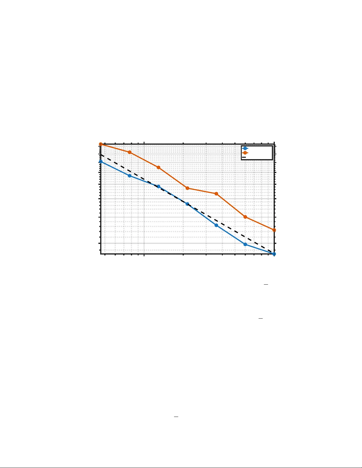
Original Paper
Loading high-quality paper...
Comments & Academic Discussion
Loading comments...
Leave a Comment