Progressive Per-Branch Depth Optimization for DEFOM-Stereo and SAM3 Joint Analysis in UAV Forestry Applications

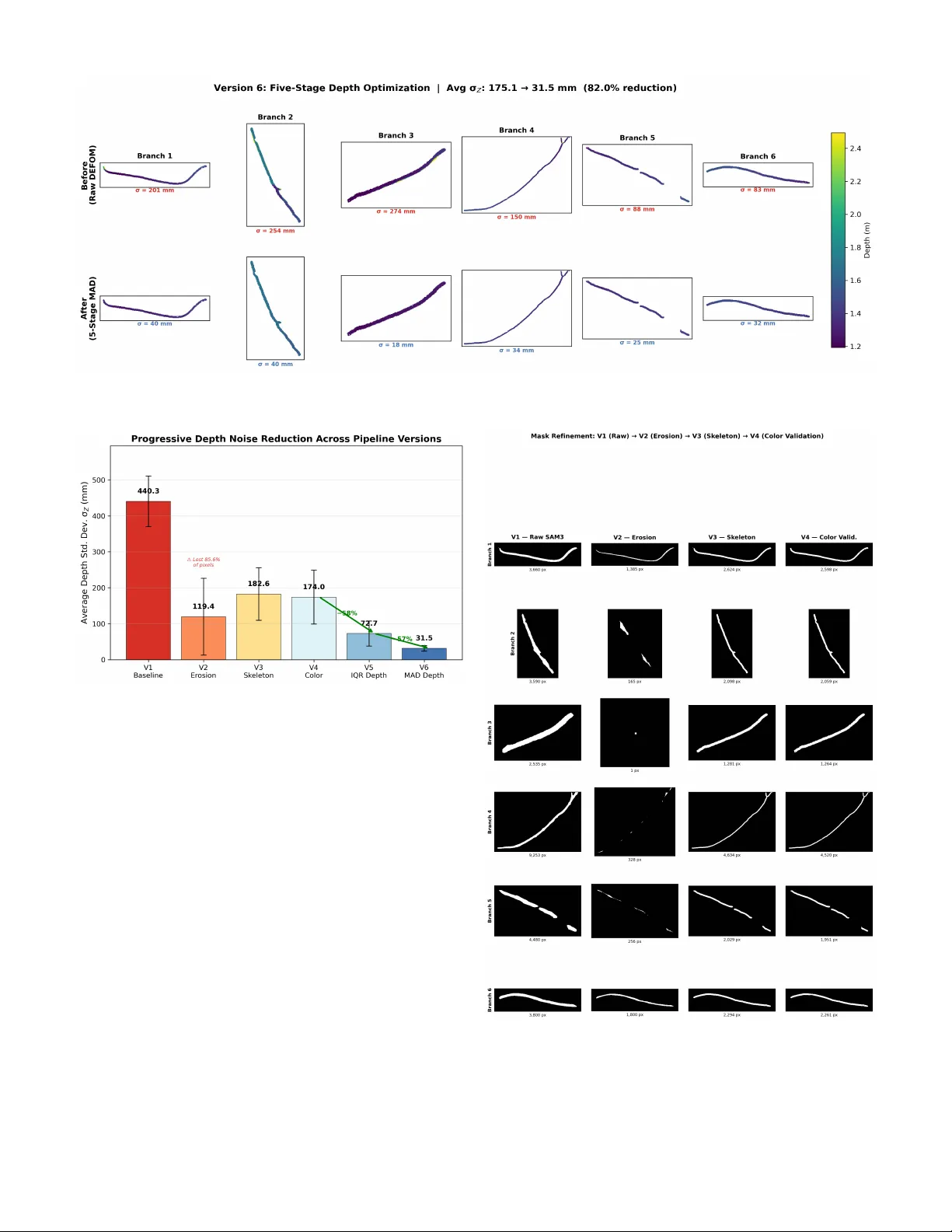
Progressi v e Per -Branch Depth Optimization for DEFOM-Stereo and SAM3 Joint Analysis in U A V F orestry Applications Y ida Lin, Bing Xue, Mengjie Zhang Centr e for Data Science and Artificial Intelligence V ictoria University of W ellington, W ellington, New Zealand linyida @ myvuw .ac.nz, bing.xue @ vuw .ac.nz, mengjie.zhang @ vuw .ac.nz Sam Schofield, Richard Green Department of Computer Science and Softwar e Engineering University of Canterb ury , Canterbury , New Zealand sam.schofield @ canterbury .ac.nz, richard.green @ canterbury .ac.nz Abstract —Accurate per -branch 3D reconstruction is a pre- requisite for autonomous U A V -based tree pruning, yet dense disparity maps from moder n stereo matchers r emain too noisy for individual branch analysis in complex forest canopies. This paper introduces a pr ogressi ve pipeline that chains DEFOM- Stereo foundation-model disparity estimation, SAM3 instance segmentation, and multi-stage depth optimization to deliver rob ust per -branch point clouds. Beginning with a na ¨ ıve baseline (V ersion 1), we identify and resolve three error families across six successive r efinements. Mask boundary contamination is first tackled through mor phological erosion (V ersion 2) and subse- quently through a skeleton-pr eserving variant that safeguards thin-branch topology (V ersion 3). Segmentation inaccuracy is then addressed with LAB-space Mahalanobis color validation coupled with cross-branch o verlap arbitration (V ersion 4). Depth noise—the final and most persistent error source—is initially mitigated by IQR/Z-score outlier removal and median filtering (V ersion 5), befor e being superseded by a fiv e-stage robust scheme: MAD global detection, spatial density consensus, local MAD filtering, RGB-guided filtering, and adaptive bilateral filtering (V ersion 6). Evaluated on 1920 × 1080 stereo imagery of Radiata pine acquired with a ZED Mini camera (63 mm baseline) from a U A V in Canterbury , New Zealand, the final pipeline reduces average per -branch depth standard de viation by 82% while retaining edge fidelity—yielding geometrically coherent 3D point clouds ready for autonomous pruning tool positioning. All code and processed outputs are publicly released to facilitate further U A V forestry resear ch. Index T erms —Stereo matching, depth optimization, instance segmentation, U A V for estry , 3D reconstruction, point cloud, tree branch I . I N T RO D U C T I O N Radiata pine ( Pinus radiata ) dominates New Zealand’ s plantation landscape, underpinning a forestry sector worth NZ$3.6 billion (1.3% of GDP). Producing high-value clear wood demands re gular pruning, yet the manual process ex- poses workers to serious hazards—falls and chainsaw in- juries chief among them. Autonomous U A V -based pruning promises a safer pathway [1], [2], b ut its realization hinges on centimeter-le vel depth knowledge per individual branch at 1–2 m operating distances. The con ver gence of two recent breakthroughs no w makes per-branch 3D reconstruction from drone stereo imagery a practical prospect. On the depth side, DEFOM-Stereo [4]— a foundation model coupling a DINOv2 [10] V iT -L encoder with iterative stereo decoding—delivers state-of-the-art cross- domain generalization, producing dense disparity maps on unseen vegetation scenes without fine-tuning [3]. On the segmentation side, the Segment Anything Model 3 (SAM3) [5] provides class-agnostic instance masks that reliably delineate individual branches despite heavy occlusion. Chaining these two components opens the door to extracting per-branch depth maps and reconstructing 3D point clouds—a capability that neither stereo-only nor segmentation-only pipelines can offer alone. In practice, howe ver , a straightforward fusion of DEFOM and SAM3 e xposes three interacting error sources that se verely compromise per-branch 3D fidelity . First, SAM3 masks tend to extend slightly past true branch contours, admitting back- ground (sky) pixels with drastically different depth values— what we refer to as mask boundary contamination . Second, confidence-based filtering is insufficient to pre vent color- inconsistent pix els from infiltrating branch masks or to dis- entangle overlapping masks between neighboring branches ( segmentation inaccuracy ). Third, DEFOM disparity maps, although globally accurate, harbor per-pixel noise, spatially isolated outliers, and boundary artif acts that corrupt per -branch depth histograms and 3D reconstructions ( depth noise ). Rather than attempting a monolithic solution, we adopt a pr ogr essive strate gy: six successiv e pipeline versions, each diagnosing and correcting a specific failure mode surfaced by its predecessor . • V ersion 1 (Baseline) directly chains DEFOM disparity estimation, depth con version, SAM3 segmentation, and per-branch point cloud generation; no refinement is ap- plied. • V ersions 2–3 attack mask boundary contamination— first with standard morphological erosion (V2), then with a skeleton-preserving variant that maintains thin- branch connectivity via distance transforms and topolog- ical skeletonization (V3). • V ersion 4 targets segmentation inaccuracy through a four-stage refinement sequence: boundary erosion with skeleton connectivity , LAB Mahalanobis color validation, connected-component cleaning, and cross-branch overlap arbitration. • V ersion 5 addresses depth noise via multi-round IQR outlier remov al, Z-score filtering, local spatial detection, and median smoothing. • V ersion 6 (Final) supersedes V5 with a more robust fiv e-stage depth pipeline: MAD global outlier detection, spatial density consensus, local MAD filtering, RGB- guided filtering [15], and adaptiv e bilateral filtering. The principal contrib utions of this work are as follows: • The first end-to-end pipeline uniting a stereo foundation model (DEFOM) with instance segmentation (SAM3) for per-branch 3D reconstruction in forestry . • A skeleton-preserving mask erosion algorithm that pro- tects thin-branch topology during boundary refinement. • A LAB Mahalanobis color-v alidation scheme enabling pixel-le vel segmentation verification and cross-branch ov erlap resolution. • A fi ve-stage robust depth optimization pipeline that inte- grates MAD statistics, spatial consensus, guided filtering, and adapti ve bilateral filtering for edge-preserving depth denoising. • A systematic ablation study quantifying each refinement stage’ s contribution to final per-branch 3D quality . I I . R E L A T E D W O R K A. Deep Ster eo Matching and F oundation Models End-to-end trainable architectures hav e reshaped stereo matching over the past decade. Spatial pyramid pooling for multi-scale cost aggregation (PSMNet [7]), group-wise correlation volumes (GwcNet [8]), and iterati ve refinement borrowed from optical flo w (RAFT -Stereo [9]) represent suc- cessiv e leaps in disparity quality . A more recent paradigm shift tow ards foundation models prioritizes cross-domain robustness ov er benchmark-specific accuracy . DEFOM-Stereo [4] exem- plifies this trend: by pairing a DINOv2 [10] V iT -L encoder with iterative stereo decoding, it achiev es state-of-the-art zero- shot performance across ETH3D [11], KITTI [12], and Mid- dlebury [13]—deliv ering consistent disparity maps with no catastrophic failures. Its suitability for ve getation scenes was confirmed in our earlier benchmark study [3], which motiv ates its adoption as the depth front-end here. B. Instance Se gmentation for V eg etation Promptable, class-agnostic segmentation became widely ac- cessible through the Segment Anything Model (SAM) [6]. Its successor , SAM 2 [5], introduced memory-augmented transformers for video-level reasoning, while SAM3 further sharpens mask boundaries through multi-scale feature fusion. Forestry applications ha ve thus far concentrated on indi vidual tree cro wn delineation [25]; per -branc h segmentation and the do wnstream depth e xtraction it enables remain largely uncharted territory . C. Depth Map Refinement and Filtering Stereo disparity maps are well known to suffer from noise, outliers, and edge bleeding. Bilateral filtering [16], guided filtering [15], and weighted median filtering [17] constitute Stereo Input DEFOM- Stereo Depth Conversion SAM3 V iT -L DINOv2 Z = f B/d s k > 0 . 7 V1 Baseline V2–V3 Mask Erosion V4 Color V alid. V5–V6 Depth Opt. Skeleton pres. LAB Mahal. MAD + Guided 3D Point Cloud Fig. 1: Overview of the progressive pipeline. Foundation modules (top, blue) feed into SAM3; the arrow descends to V ersion 1, then proceeds right-to-left through six iterative refinements (orange) ad- dressing mask contamination (V2–V3), segmentation accuracy (V4), and depth noise (V5–V6), producing per-branch 3D point clouds. the classical arsenal for alleviating these artifacts. On the statistical front, IQR- and MAD-based outlier detection [18] is standard practice in robust statistics, yet its spatially adaptiv e, per-instance application to stereo depth remains uncommon. Our pipeline traces an evolution from basic IQR clipping to a composite fiv e-stage strategy that weav es together global MAD, local spatial consensus, guided filtering, and adaptiv e bilateral filtering. D. Ster eo V ision for U A V F or estry Drone-mounted stereo cameras have been deployed for navigation [21], 3D reconstruction [22], and obstacle a void- ance [23]. More closely aligned with our goals, recent efforts in branch detection [1], [24] and segmentation [25] illus- trate how deep learning and stereo vision can jointly serve forestry needs. What remains missing is a pipeline that fuses foundation-model stereo with instance se gmentation for per- branch 3D point cloud generation. The present work fills precisely this gap, offering a complete pathway from raw stereo pairs to optimized per-branch point clouds. I I I . M E T H O D O L O G Y An overvie w of the complete pipeline appears in Fig. 1. The subsections below first lay out the shared foundation modules (§III-A) and then walk through each refinement stage in the order it w as de veloped (§III-B–§III-G). A. Shar ed F oundation 1) Data Acquisition: W e capture stereo image pairs at 1920 × 1080 resolution using a ZED Mini camera ( f x ≈ 1120 px, baseline B = 63 mm) mounted on a U A V . Images are captured at 1–2 m distance from Radiata pine branches in Canterbury , New Zealand, under varying illumination condi- tions (March–October 2024). Fig. 2 shows a representativ e left image and the corresponding DEFOM-Stereo disparity map. 2) DEFOM-Ster eo Disparity Estimation: Giv en a rectified stereo pair ( I L , I R ) ∈ R H × W × 3 , DEFOM-Stereo produces a dense disparity map D ∈ R H × W . The model uses a DINOv2 V iT -L encoder with 32 valid iterations and 8 scale iterations. From disparity , depth is recov ered by triangulation: Z ( x, y ) = f x · B D ( x, y ) (1) (a) Left stereo image (b) DEFOM disparity Fig. 2: Representativ e input data: (a) left image of Radiata pine canopy captured by ZED Mini at 1–2 m, and (b) dense disparity map produced by DEFOM-Stereo (V iT -L DINOv2, 32 iterations). W arm colors indicate closer objects. where f x is the horizontal focal length and B is the stereo baseline. 3) 3D P oint Cloud Generation: Each pixel ( u, v ) with v alid depth Z is back-projected to 3D using the standard pinhole model: X = ( u − c x ) · Z f x , Y = ( v − c y ) · Z f y (2) where ( c x , c y ) are the principal point coordinates. The result- ing point cloud P = { ( X i , Y i , Z i , R i , G i , B i ) } preserves RGB color from the left image. 4) SAM3 Instance Se gmentation: SAM3 is applied to the left image to produce a set of branch masks { M k } K k =1 with confidence scores { s k } . Only masks with s k > 0 . 7 are retained. For each accepted mask M k , the per-branch depth map is Z k = Z ⊙ M k (element-wise masking). B. V ersion 1: Baseline Pipeline In its simplest form the pipeline is a straightforward cascade: DEFOM disparity → depth conv ersion → SAM3 segmentation → per-branch depth extraction and point cloud generation, with no post-processing of any kind. Although this baseline is functionally complete, it is af- flicted by all three error families simultaneously: sky-depth outliers bleed into branch histograms through imprecise mask boundaries, color -inconsistent pixels pollute SAM3 masks, and raw DEFOM noise scatters points across the 3D reconstruc- tions. C. V ersion 2: Morphological Mask Er osion The most immediate remedy for boundary contamination is to shrink each SAM3 mask inward before e xtracting depth. V ersion 2 accomplishes this with morphological erosion using an elliptical structuring element of radius r e = 15 px: M eroded k = M k ⊖ E r e (3) where ⊖ denotes morphological erosion and E r e is the struc- turing element. A fallback mechanism progressively reduces r e to { r e / 2 , r e / 4 , 3 , 1 } if the erosion destroys the mask entirely (i.e., | M eroded k | = 0 ). Limitation : Standard morphological erosion works well for thick branches but disconnects or entirely removes thin branches whose diameter falls below 2 r e —a shortcoming that V ersion 3 specifically tar gets. D. V ersion 3: Skeleton-Pr eserving Er osion T o retain thin-branch connecti vity , V ersion 3 introduces a topology-aware erosion strategy that fuses distance-transform erosion with topological skeletonization: Step 1: Distance transform erosion . Compute the Eu- clidean distance transform D ( x, y ) of the binary mask M k , yielding the distance from each foreground pixel to the nearest boundary . Retain only pixels suf ficiently far from the bound- ary: M dist k = { ( x, y ) : D ( x, y ) ≥ r e } (4) Step 2: T opological skeletonization . Extract the morpho- logical skeleton S ( M k ) of the original mask using the algo- rithm from [20]. The skeleton is a one-pixel-wide connected centerline that preserv es the topology of the mask. Step 3: Skeleton dilation . Dilate the skeleton with a small radius r s = max(3 , r e / 4) to gi ve it pix el width: S wide k = S ( M k ) ⊕ E r s (5) Step 4: Union . The final refined mask is the union of the distance-eroded region and the widened skeleton, clipped to the original mask: M skel k = ( M dist k ∪ S wide k ) ∩ M k (6) Because the skeleton bridge persists ev en when M dist k is empty for a narrow section, thin branches are guaranteed to remain topologically connected. E. V ersion 4: Color-V alidated Se gmentation Skeleton-preserving erosion resolves boundary geometry , yet SAM3 masks may still contain color-inconsistent pixels— foliage fragments attached to a branch mask, for instance—and neighboring masks can ov erlap. V ersion 4 tackles both issues through a four -stage segmentation refinement pipeline. 1) Stage 1: Boundary Er osion with Skeleton Preservation: Identical to V ersion 3 (Eq. 4 – 6). 2) Stage 2: LAB Mahalanobis Color V alidation: For each branch mask M k , we b uild a color model from the deeply- eroded cor e r egion C k and reject pixels whose color deviates significantly . Core region extraction : Compute the distance transform of M k and retain only inner pixels with distance ≥ r c = 25 px: C k = { ( x, y ) : D M k ( x, y ) ≥ r c } (7) If | C k | < 100 , r c is progressiv ely reduced until a sufficient core is obtained. Gaussian color model in CIELAB space : Con vert the left image to CIELAB and compute the mean µ k and cov ariance Σ k of core-region pixels: µ k = 1 | C k | X ( x,y ) ∈ C k L ( x, y ) (8) Σ k = Cov  { L ( x, y ) } ( x,y ) ∈ C k  (9) where L ( x, y ) = [ L, a, b ] T is the CIELAB vector . A regu- larization term ϵ I ( ϵ = 10 − 3 ) is added to Σ k for numerical stability . Mahalanobis distance : For each pixel in M k , compute: d M = q ( L − µ k ) T Σ − 1 k ( L − µ k ) (10) where we abbreviate L = L ( x, y ) for readability . Pixels with d M > τ M = 3 . 5 are rejected from the mask. 3) Stage 3: Connected Component Cleaning: After color validation, small disconnected fragments may remain. W e apply connected component analysis and remove components smaller than 1% of the largest component’ s area: M clean k = [ { j : | R j |≥ 0 . 01 · max j | R j |} R j (11) where R j denotes the j -th connected region. 4) Stage 4: Cr oss-Branc h Overlap Resolution: When mul- tiple masks overlap, each contested pixel is assigned to the branch whose Mahalanobis distance is smallest: k ∗ ( x, y ) = arg min k ∈O ( x,y ) d ( k ) M ( x, y ) (12) where O ( x, y ) is the set of branches claiming pixel ( x, y ) . F . V ersion 5: Statistical Depth Optimization Once segmentation has been cleaned by V ersion 4, depth noise within the DEFOM disparity map emerges as the domi- nant remaining artifact. V ersion 5 combats it with a four-phase per-branch depth optimization pipeline. 1) Phase 1: Multi-Round IQR Outlier Removal: For each branch k , compute the interquartile range of depth values within M k : IQR k = Q 3 − Q 1 (13) outlier if Z i < Q 1 − α · IQR k or Z i > Q 3 + α · IQR k with α = 1 . 5 . Outliers are replaced with the branch median ˜ Z k . This phase is applied iteratively for up to T = 3 rounds until no further outliers are detected. 2) Phase 2: Z-Score F iltering: After IQR clipping, residual outliers are detected via Z-score: z i = | Z i − ¯ Z k | σ k , outlier if z i > 2 (14) where ¯ Z k and σ k are the post-IQR branch mean and standard deviation. 3) Phase 3: Local Spatial Outlier Detection: Using a 7 × 7 sliding window , compute the local mean and standard deviation via uniform filtering: outlier if | Z i − ˜ Z local i | > β · σ local i (15) with β = 2 . 0 and ˜ Z local i denoting the local median. Detected outliers are replaced with local median v alues. 4) Phase 4: Spatial Median F iltering: A 5 × 5 median filter is applied within the mask to smooth residual noise while preserving depth edges. Limitation : Both IQR and Z-score statistics assume roughly symmetric, unimodal distributions—an assumption frequently violated on branch surfaces where partial occlusion produces bimodal depth profiles. Moreov er , the Phase 4 median filter, despite its simplicity , blurs fine-grained depth edges. V ersion 6 redesigns the entire depth pipeline to overcome these short- comings. G. V ersion 6: Advanced Robust Depth Optimization The culminating V ersion 6 discards the four-phase scheme in fav or of a fi ve-stage robust optimization, with ev ery stage engineered to address a distinct noise characteristic. T able I provides a concise ov erview . T ABLE I: Five-Stage Depth Optimization Pipeline (V ersion 6) Stage Method Purpose 1 MAD Global Robust global outlier detection 2 Spatial Density Neighbor consensus voting 3 Local MAD Local robust outlier detection 4 Guided Filter RGB-guided edge-preserving smooth 5 Adaptiv e Bilateral Depth + spatial joint weighting 1) Stage 1: MAD Global Robust Outlier Detection: The Median Absolute Deviation (MAD) [18] is a robust measure of statistical dispersion with a breakdown point of 50%, far superior to the 25% breakdown point of IQR. For each branch k , compute: MAD k = median ( | Z i − ˜ Z k | ) , i ∈ M k (16) The modified Z-scor e [19] for each pixel is: m i = 0 . 6745 · | Z i − ˜ Z k | MAD k (17) where the constant 0.6745 ensures consistency with the stan- dard deviation for Gaussian data (MAD = 0 . 6745 · σ under normality). Pixels with m i > τ MAD = 3 . 5 are classified as outliers and replaced with the branch median ˜ Z k . This stage is applied iterati vely for up to T = 3 rounds. 2) Stage 2: Spatial Density Consensus: Global MAD filter- ing captures extreme outliers but overlooks spatially isolated points whose values appear plausible in a branch-wide sense. Stage 2 introduces neighbor-consensus voting to detect such depth-inconsistent pixels: W ithin an 11 × 11 windo w , compute the local median ˜ Z loc i and local MAD. Conv ert to a robust local scale estimate: ˆ σ loc i = 1 . 4826 · MAD loc i (18) where 1.4826 is the consistency constant for a normal distri- bution. A pixel is consistent with its neighborhood if: | Z i − ˜ Z loc i | ≤ γ · ˆ σ loc i (19) with γ = 2 . 0 . The consensus ratio ρ i is the fraction of neighbors satisfying Eq. (19). A pixel is classified as an isolated outlier if it is itself inconsistent, yet its neighborhood has high consensus ( ρ i ≥ 0 . 3 ). Such outliers are replaced with ˜ Z loc i . 3) Stage 3: Local MAD Outlier Detection: Even after global and consensus-based filtering, fine-grained local noise persists. Stage 3 re-applies MAD-based detection at the local scale, operating within a 7 × 7 window: | Z i − ˜ Z loc i | > τ L · 1 . 4826 · MAD loc i (20) with τ L = 3 . 0 . Because the local MAD is inherently insensi- tiv e to the very outliers it seeks to identify , it provides a more reliable scale estimate than the standard-de viation approach of V ersion 5. 4) Stage 4: Guided F ilter: Edge-preserving smoothing is realized through the guided filter [15], which leverages the RGB image as a structural reference. Gi ven guidance image I and input depth p , the output at pixel i is: q i = ¯ a k · I i + ¯ b k (21) where ¯ a k and ¯ b k are av eraged linear coefficients computed as: a k = 1 | ω k | P i ∈ ω k I i p i − ¯ I k ¯ p k σ 2 k + ϵ (22) b k = ¯ p k − a k ¯ I k with windo w ω k of radius r = 4 and re gularization ϵ = 0 . 01 . W e construct a multi-channel guidance signal by combining grayscale intensity , and CIELAB L, a, b channels with weights [0 . 4 , 0 . 3 , 0 . 15 , 0 . 15] , ensuring that both luminance and chromi- nance edges are respected during depth smoothing. 5) Stage 5: Adaptive Bilateral F iltering: A final bilateral filtering pass combines spatial proximity and depth similarity into a joint weighting scheme with data-adaptive parameters. The filtered depth at pixel i is: q i = P j ∈N i w s ( i, j ) · w d ( i, j ) · Z j P j ∈N i w s ( i, j ) · w d ( i, j ) (23) where w s ( i, j ) = exp( −∥ p i − p j ∥ 2 / 2 σ 2 s ) is the spatial weight and w d ( i, j ) = exp( −| Z i − Z j | 2 / 2 σ 2 d ) is the depth-range weight. Critically , the depth-range bandwidth σ d is automatically tuned per branch using the branch’ s o wn MAD: σ d = α d · 1 . 4826 · MAD k (24) with α d = 1 . 5 and spatial bandwidth σ s = 7 px. This adap- tation ensures that branches with larger depth variation (e.g., trunks) receiv e broader smoothing, while thin branches with tight depth distrib utions receive more conservati ve filtering. I V . E X P E R I M E N TA L R E S U L T S A. Experimental Setup Hardwar e : All experiments run on Google Colab with NVIDIA A100/V100 GPU. DEFOM-Stereo uses a V iT -L DINOv2 backbone with 32 valid iterations. Data : W e process stereo pairs of Radiata pine branches at 1920 × 1080 resolution captured with a ZED Mini camera (focal length f x ≈ 1120 px, baseline B = 63 mm). Evaluation metrics : W e ev aluate per-branch depth quality using: • Depth standard deviation ( σ Z ): lo wer values indicate less noise within a single branch. • Depth range (max − min): smaller ranges indicate fewer extreme outliers and tighter per-branch distributions. • T otal mask pixels : retained mask area; a drop indicates loss of thin structures. • 3D point cloud coherence : qualitati vely assessed via per - branch colored point clouds and depth histograms. B. V ersion-by-V ersion Comparison T able II summarizes the progressiv e improvement across all six versions. Fig. 4 visualizes the average depth standard deviation reduction. C. Mask Refinement Analysis (V1–V4) V1 → V2 : The mask refinement progression from V1 to V4 is laid out in Fig. 5. Shrinking each mask inward by 15 px strips aw ay the majority of sky-pixel outliers from depth T ABLE II: Progressive Improvement Across Pipeline V ersions V er . A vg. σ Z (mm) Range (mm) Pixels Mask Qual. Thin Br . V1 (Baseline) 440.3 1545 27 318 Low N/A V2 (Erosion) 119.4 461 3 935 Medium No V3 (Skeleton) 182.6 1431 14 960 Medium Y es V4 (Color) 174.0 1431 14 653 High Y es V5 (IQR) 72.7 281 14 653 High Y es V6 (MAD) 31.5 128 14 665 High Y es A vg. σ Z and A vg. Range are av eraged across all six branches. T otal Pixels is the sum of valid mask pixels across branches. V2 loses 85.6% of pixels due to na ¨ ıve erosion. V5 and V6 share V4’ s masks but apply depth optimization. histograms. The cost, howe ver , is severe: thin branches whose diameter falls below 30 px are disconnected or lost entirely . V2 → V3 : Skeleton-preserving erosion reco vers this lost connectivity . By extracting the topological centerline and dilating it to r s = max(3 , r e / 4) pixels before merging with the distance-eroded mask, the algorithm eliminates topology loss while retaining boundary erosion for larger structures. V3 → V4 : Geometric refinement alone cannot catch pixels that lie within the mask boundary yet differ in color from the branch. The LAB Mahalanobis color model (Eq. 9) built from the deeply-eroded core provides a robust reference, and the τ M = 3 . 5 threshold strikes a balance between tolerating natural color variability and excising contaminants. Subse- quent cross-branch ov erlap resolution (Eq. 12) produces the non-ov erlapping masks required for unbiased per-branch depth statistics. D. Depth Optimization Analysis (V5–V6) Per-branch depth distrib utions before and after the V ersion 6 optimization are contrasted in Fig. 6. V4 → V5 : Applying the four-phase IQR-based pipeline yields a marked reduction in depth noise. Gross outliers are clipped by multi-round IQR; residual large deviations fall to Z-score filtering; isolated local noise is caught by spatial detection; and a final median pass smooths what remains. A notable drawback is that the 5 × 5 median kernel blurs depth edges, and the 25% breakdown point of IQR means that extreme outliers can still inflate Q 1 /Q 3 enough to escape detection. V5 → V6 : The five-stage MAD-based pipeline (Fig. 3) ov ercomes each of these limitations: 1) MAD vs. IQR : W ith a 50% breakdown point, MAD can tolerate outliers constituting up to half the data, far exceeding IQR’ s 25% ceiling. 2) Consensus voting vs. Z-score : Neighborhood agree- ment captures spatially isolated anomalies that global statistics ov erlook. 3) Guided filter vs. median filter : By respecting RGB- aligned depth discontinuities, the guided filter retains sharper branch boundaries in 3D. 4) Adaptive bilateral smoothing : Branch-specific σ d tun- ing (Eq. 24) scales the smoothing bandwidth to each branch’ s depth variability , prev enting ov er-smoothing of narrow branches and under -smoothing of wide trunks. Fig. 3: V ersion 6 fi ve-stage depth optimization results. T op row: before optimization (V4 masks with raw DEFOM depth). Bottom row: after the fiv e-stage MAD-based pipeline. A verage σ Z reduced from 174.6 mm to 31.5 mm (82.0% reduction). Fig. 4: A verage per-branch depth standard deviation across pipeline versions. V2 achiev es low σ Z but loses 85.6% of mask pixels. V6 achiev es the lowest σ Z (31.5 mm) while preserving all branches. E. 3D P oint Cloud Quality Across pipeline versions, 3D point cloud fidelity improves substantially (Fig. 7). V ersion 1 clouds are dominated by scatter originating from both mask contamination and depth noise. Mask-related scatter disappears by V ersion 4, though depth-noise scatter persists. V ersion 5 curbs depth noise at the expense of edge blur . V ersion 6 strikes the most fa vorable balance: depth values cluster tightly within each branch, boundaries remain sharp where the y coincide with RGB edges, and isolated outlier points are nearly absent. The final RGB- textured per-branch point cloud is shown in Fig. 8. F . P er-Branc h Depth Distrib ution Analysis Box plots (Fig. 9) e xpose the cumulativ e impact of each refinement on per-branch depth distributions. V ersion 1 ex- hibits extreme outliers—driven by sky-depth contamination— and wide IQR ranges. Successive mask refinements (V2– V4) progressively purge distribution contamination, while the depth optimization stages (V5–V6) further compress the IQR Fig. 5: Mask refinement progression from V1 to V4. V2 erosion disconnects thin branches (Branch 3: 2 535 → 1 px). V3 skeleton preservation recovers connectivity (1 281 px). V4 color validation produces clean masks. Fig. 6: Per-branch depth optimization comparison (V ersion 6). Before (top) vs. after (bottom) the fi ve-stage pipeline, showing distribution narrowing and outlier elimination for each branch. T ABLE III: Per-Branch Depth Optimization: V5 vs. V6 Branch Befor e σ Z V5 σ Z V6 σ Z V6 Red. (mm) (mm) (mm) (%) B1 ( N =2 598) 201.7 91.7 39.7 80.3 B2 ( N =2 059) 252.7 137.9 39.9 84.2 B3 ( N =1 264) 274.9 35.4 17.6 93.6 B4 ( N =4 520) 146.9 65.3 34.4 76.6 B5 ( N =1 951) 84.5 37.6 24.9 70.5 B6 ( N =2 261) 86.9 68.3 32.4 62.7 A verage 174.6 72.7 31.5 82.0 “Before” is the V4-refined mask without depth optimization. V5 uses IQR+Z-score+median filter (1 738 pixels modified). V6 uses MAD+spatial consensus+guided+bilateral filter (4 623 pixels modified). Reduction computed relative to Before. and eliminate residual whiskers, ultimately yielding per -branch depth estimates precise enough for centimeter-le vel tool posi- tioning. G. Ablation Study: Depth Optimization Stages T o isolate the contribution of depth optimization from mask refinement, T able III compares V ersion 5 (IQR-based) and V ersion 6 (MAD-based) starting from identical V4-refined masks. V . D I S C U S S I O N A. Rationale for Pr ogr essive Refinement The six-version arc is not mere incremental tinkering; it is a diagnostic sequence in which every version exposes a distinct failure mode that shapes the subsequent design decision: • V ersion 1 uncovered the inadequacy of SAM3’ s boundary precision for depth-sensitive tasks, pointing to the need for mask erosion. • The thin-branch topology destruction caused by na ¨ ıve erosion in V ersion 2 prompted the skeleton-preserving strategy of V ersion 3. • V ersion 3 made clear that geometry-only mask refine- ment leav es color-inconsistent pixels intact, necessitating Mahalanobis color v alidation. • With mask quality secured, V ersion 4 exposed depth noise as the single largest obstacle to accurate per-branch reconstruction. • V ersion 5’ s reliance on IQR and Z-score proved fragile under the heavy-tailed noise distrib utions typical of v eg- etation stereo, driving the redesign around MAD-based statistics. This chain of diagnoses guarantees that e very component is both necessary —removing it measurably degrades output quality—and tar geted at a genuinely differ ent failur e mode . B. Robustness of MAD vs. IQR Switching from IQR-based (V ersion 5) to MAD-based (V er- sion 6 Stage 1) outlier detection rests on a clear theoreti- cal foundation: the br eakdown point —the largest fraction of outliers a statistic can tolerate before its estimate becomes arbitrarily unreliable. IQR breaks down at 25%: once more than a quarter of depth values are corrupted, Q 1 and Q 3 themselves become distorted. MAD, by contrast, withstands contamination of up to 50% of the data. In forestry imagery , branches frequently occupy only a minor share of the mask area—particularly after partial occlusion—making the doubled resilience of MAD a decisiv e practical adv antage. C. Edge Pr eservation: Guided F ilter vs. Median F ilter Replacing the median filter (V ersion 5) with an RGB-guided filter (V ersion 6 Stage 4) tackles a core deficiency: median filtering is spatially isotropic and blind to image structure. The guided filter , in contrast, borrows edge information from the color image, preserving depth discontinuities wherever the y align with color transitions. For tree branches—where the depth boundary and the branch-background color boundary are essentially co-located—this property is especially valuable. D. Practical Implications Beyond noise reduction, the V ersion 6 pipeline unlocks sev- eral do wnstream capabilities critical for autonomous pruning: • Branch diameter estimation : T ighter depth distribu- tions support reliable depth-profile analysis for measuring branch cross-sections. • Pruning path planning : Geometrically clean per-branch point clouds furnish the spatial input needed by cutting- tool trajectory optimizers. • Distance estimation : Narrow per-branch depth distribu- tions translate directly into precise U A V -to-branch dis- tance readings during approach maneuvers. E. Limitations Pseudo-Ground-T ruth Ceiling. Depth accuracy is funda- mentally capped by DEFOM-Stereo’ s disparity estimation. Prediction errors in textureless sky regions or heavily occluded areas propagate through ev ery subsequent optimization stage. Parameter Sensitivity . The pipeline relies on se veral hand- tuned parameters ( τ M , τ MAD , r e , r c , ϵ , α d ). Although the chosen v alues generalize well within our test scenes, different tree species or camera configurations may demand re-tuning. Computational Cost. DEFOM-Stereo inference dominates the overall runtime; the added mask refinement and depth optimization stages contrib ute negligible ov erhead. Fig. 7: Per-branch 3D point cloud progression from V1 to V6. V ersion 1 exhibits sev ere scatter from mask contamination and depth noise. V ersion 4 removes mask-related scatter. V ersion 6 achiev es tight depth clustering with minimal outliers. Fig. 8: Final V ersion 6 RGB-textured per -branch point cloud. Each branch is color-coded; clean geometry is suitable for autonomous pruning path planning. Fig. 9: Box plots comparing per -branch depth distributions across pipeline versions. V ersion 6 shows the tightest distributions with the fewest outliers. Limited Scene Diversity . All e xperiments in volve Radiata pine in Canterb ury , New Zealand. Broader validation across species, seasons, and lighting conditions remains necessary . V I . C O N C L U S I O N This paper introduced a progressiv e pipeline that unites DEFOM-Stereo disparity estimation, SAM3 instance segmen- tation, and multi-stage depth optimization for per-branch 3D reconstruction in U A V forestry . Over six successi ve versions, three distinct error families were identified and resolved: mask boundary contamination through skeleton-preserving erosion, segmentation inaccuracy through LAB Mahalanobis color v alidation, and depth noise through a fiv e-stage MAD- based robust optimization augmented by guided and adaptiv e bilateral filtering. The follo wing findings stand out: • Skeleton-preserving erosion suppresses boundary con- tamination without sacrificing thin-branch connectivity , surpassing con ventional morphological erosion. • LAB Mahalanobis color validation effecti vely purges color-inconsistent pixels and arbitrates cross-branch over - laps, yielding clean, non-overlapping instance masks. • MAD-based outlier detection , with its 50% breakdown point, pro ves substantially more reliable than IQR-based methods (25% breakdown) under the heavy-tailed noise typical of v egetation depth data. • Multi-channel guided filtering respects depth discon- tinuities aligned with RGB edges, deliv ering sharper branch reconstructions than isotropic median filtering. • Adaptive bilateral filtering tunes σ d per branch, match- ing smoothing intensity to each branch’ s intrinsic depth variability . T aken together , these refinements produce geometrically coherent per-branch 3D point clouds suitable for pruning path planning, branch diameter measurement, and real-time distance computation. Code, processed outputs, and interactiv e 3D visualizations are publicly released. Looking ahead, we plan to couple this pipeline with branch detection [1] and seg- mentation [25] systems toward fully autonomous pruning, and to e xplore temporal consistency constraints enabling video-rate per-branch tracking. A C K N O W L E D G M E N T S This research was supported by the Royal Society of New Zealand Marsden Fund and the Ministry of Business, Innov a- tion and Employment. W e thank the forestry research stations for data collection access. R E F E R E N C E S [1] Y . Lin, B. Xue, M. Zhang, S. Schofield, and R. Green, “Deep learning- based depth map generation and YOLO-integrated distance estimation for radiata pine branch detection using drone stereo vision, ” in Proc. Int. Conf. Imag e V is. Comput. New Zealand (IVCNZ) , Christchurch, New Zealand, 2024, pp. 1–6. [2] D. Steininger, J. Simon, A. Trondl, and M. Murschitz, “TimberV ision: A multi-task dataset and framew ork for log-component segmentation and tracking in autonomous forestry operations, ” in Pr oc. IEEE/CVF W inter Conf. Appl. Comput. V is. (W ACV) , 2025. [3] Y . Lin, B. Xue, M. Zhang, S. Schofield, and R. Green, “T owards gold- standard depth estimation for tree branches in U A V forestry: Benchmark- ing deep stereo matching methods, ” arXiv pr eprint arXiv:2601.19461 , 2026. [4] H. Jiang, Z. Lou, L. Ding, R. Xu, M. T an, W . Jiang, and R. Huang, “DEFOM-Stereo: Depth foundation model based stereo matching, ” arXiv preprint arXiv:2501.09466 , 2025. [5] N. Ravi, V . Gabeur , Y .-T . Hu, R. Hu, C. Ryali, T . Ma, H. Khedr, R. R ¨ adle, C. Rolland, L. Gustafson, E. Mintun, J. P an, K. V . Alwala, N. Carion, C.-Y . W u, R. Girshick, P . Doll ´ ar , and C. Feichtenhofer , “SAM 2: Segment an ything in images and videos, ” arXiv pr eprint arXiv:2408.00714 , 2024. [6] A. Kirillov , E. Mintun, N. Ravi, H. Mao, C. Rolland, L. Gustafson, T . Xiao, S. Whitehead, A. C. Berg, W .-Y . Lo, P . Doll ´ ar , and R. Girshick, “Segment anything, ” in Proc. IEEE Int. Conf. Comput. V is. (ICCV) , 2023, pp. 4015–4026. [7] J.-R. Chang and Y .-S. Chen, “Pyramid stereo matching network, ” in Pr oc. IEEE Conf. Comput. V is. P attern Recognit. (CVPR) , 2018, pp. 5410–5418. [8] X. Guo, K. Y ang, W . Y ang, X. W ang, and H. Li, “Group-wise correlation stereo network, ” in Pr oc. IEEE Conf. Comput. V is. P attern Recognit. (CVPR) , 2019, pp. 3273–3282. [9] L. Lipson, Z. T eed, and J. Deng, “RAFT -Stereo: Multilev el recurrent field transforms for stereo matching, ” in Proc. Int. Conf. 3D V is. (3D V) , 2021, pp. 218–227. [10] M. Oquab, T . Darcet, T . Moutakanni, H. V o, M. Szafraniec, V . Khalidov , P . Fernandez, D. Haziza, F . Massa, A. El-Nouby , M. Assran, N. Ballas, W . Galuba, R. Howes, P .-Y . Huang, S.-W . Li, I. Misra, M. Rabbat, V . Sharma, G. Synnaev e, H. Xu, H. Jegou, J. Mairal, P . Labatut, A. Joulin, and P . Bojanowski, “DINOv2: Learning robust visual features without supervision, ” T rans. Mach. Learn. Res. , 2024. [11] T . Sch ¨ ops, J. L. Sch ¨ onberger , S. Galliani, T . Sattler , K. Schindler , M. Pollefeys, and A. Geiger, “ A multi-view stereo benchmark with high-resolution images and multi-camera videos, ” in Proc. IEEE Conf. Comput. V is. P attern Recognit. (CVPR) , 2017, pp. 2538–2547. [12] A. Geiger, P . Lenz, and R. Urtasun, “ Are we ready for autonomous driving? The KITTI vision benchmark suite, ” in Pr oc. IEEE Conf. Comput. V is. P attern Recognit. (CVPR) , 2012, pp. 3354–3361. [13] D. Scharstein, H. Hirschm ¨ uller , Y . Kitajima, G. Krathwohl, N. Ne ˇ si ´ c, X. W ang, and P . W estling, “High-resolution stereo datasets with subpixel- accurate ground truth, ” in Pr oc. German Conf. P attern Recognit. (GCPR) , 2014, pp. 31–42. [14] N. Mayer, E. Ilg, P . Hausser, P . Fischer, D. Cremers, A. Dosovitskiy , and T . Brox, “ A large dataset to train con volutional networks for disparity , optical flow , and scene flow estimation, ” in Pr oc. IEEE Conf. Comput. V is. P attern Recognit. (CVPR) , 2016, pp. 4040–4048. [15] K. He, J. Sun, and X. T ang, “Guided image filtering, ” IEEE Tr ans. P attern Anal. Mach. Intell. , vol. 35, no. 6, pp. 1397–1409, Jun. 2013. [16] C. T omasi and R. Manduchi, “Bilateral filtering for gray and color images, ” in Pr oc. IEEE Int. Conf. Comput. V is. (ICCV) , 1998, pp. 839– 846. [17] Z. Ma, K. He, Y . W ei, J. Sun, and E. Wu, “Constant time weighted median filtering for stereo matching and beyond, ” in Pr oc. IEEE Int. Conf. Comput. V is. (ICCV) , 2013, pp. 49–56. [18] C. Leys, C. Ley , O. Klein, P . Bernard, and L. Licata, “Detecting outliers: Do not use standard deviation around the mean, use absolute deviation around the median, ” J. Exp. Social Psych. , vol. 49, no. 4, pp. 764–766, 2013. [19] B. Iglewicz and D. C. Hoaglin, V olume 16: How to Detect and Handle Outliers . Milwaukee, WI: ASQC Quality Press, 1993. [20] T .-C. Lee, R. L. Kashyap, and C.-N. Chu, “Building skeleton models via 3-D medial surface/axis thinning algorithms, ” CVGIP: Gr aph. Models Image Pr ocess. , vol. 56, no. 6, pp. 462–478, 1994. [21] F . Fraundorfer , L. Heng, D. Honegger , G. H. Lee, L. Meier, P . T anskanen, and M. Pollefeys, “V ision-based autonomous mapping and exploration using a quadrotor MA V , ” in Pr oc. IEEE/RSJ Int. Conf. Intell. Robots Syst. (IROS) , 2012, pp. 4557–4564. [22] F . Nex and F . Remondino, “U A V for 3D mapping applications: A revie w , ” Appl. Geomat. , vol. 6, no. 1, pp. 1–15, 2014. [23] A. J. Barry and R. T edrake, “Pushbroom stereo for high-speed navigation in cluttered en vironments, ” in Pr oc. IEEE Int. Conf. Robot. Autom. (ICRA) , 2015, pp. 3046–3052. [24] Y . Lin, B. Xue, M. Zhang, S. Schofield, and R. Green, “YOLO and SGBM integration for autonomous tree branch detection and depth estimation in radiata pine pruning applications, ” in Proc. Int. Conf. Image V is. Comput. Ne w Zealand (IVCNZ) , W ellington, New Zealand, 2025, pp. 1–6. [25] Y . Lin, B. Xue, M. Zhang, S. Schofield, and R. Green, “Performance ev aluation of deep learning for tree branch segmentation in autonomous forestry systems, ” in Pr oc. Int. Conf. Image V is. Comput. New Zealand (IVCNZ) , W ellington, New Zealand, 2025, pp. 1–6.