Waveform Design for Partial-Time Superimposed ISAC Systems

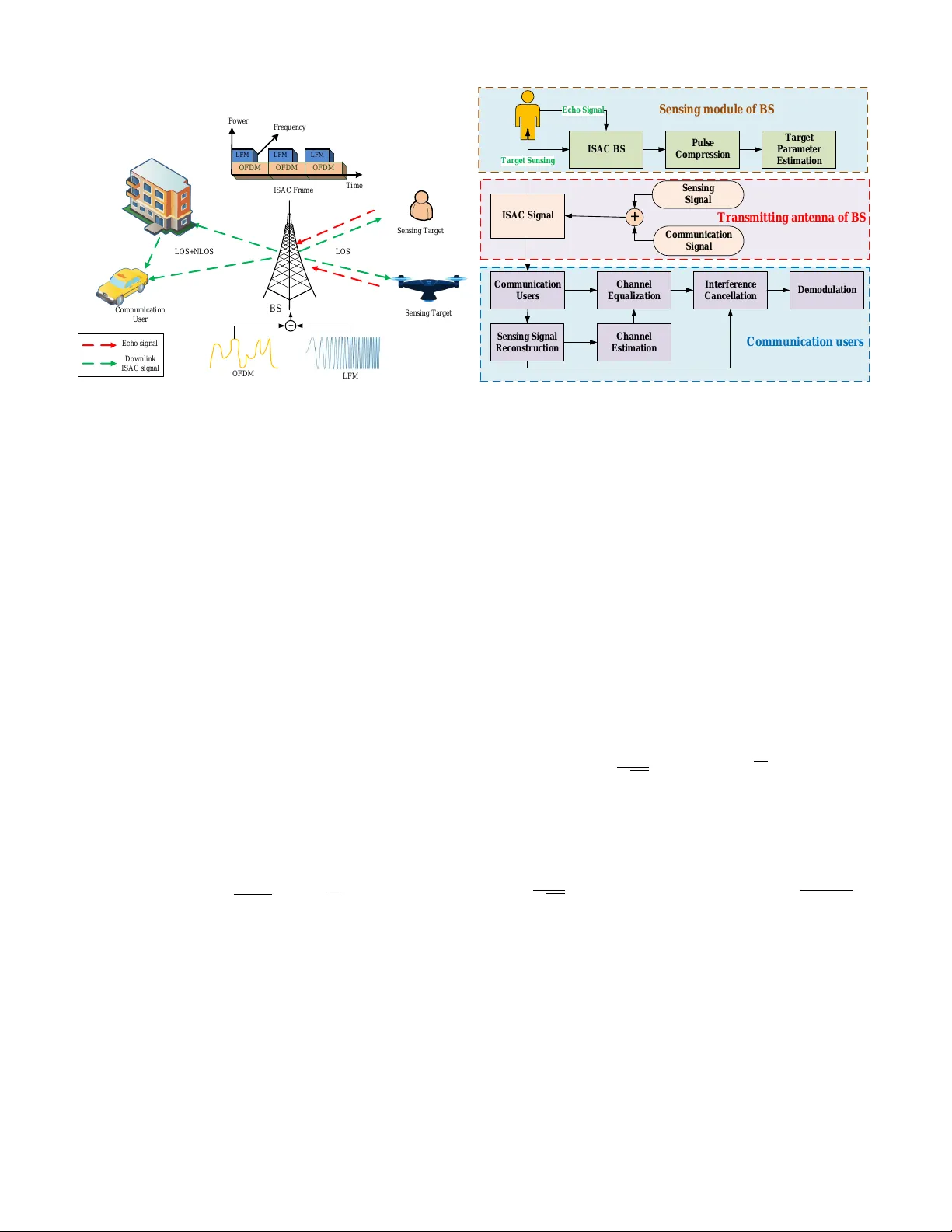
1 W a v eform Design for P artial-T ime Superimposed ISA C Systems Xi Nan, Rugui Y ao, Y e Fan, Ruikang Zhong, Xiao ya Zuo, Theodoros A. Tsiftsis and Alexandros-Apostolos A. Boulogeor gos Abstract —Nowadays, wav eforms of integrated sensing and communication (ISA C) are almost based on con ventional com- munication and sensing signal, which bounds both the commu- nication and sensing performance. T o deal with this issue, in this paper , a novel wav eform design is presented for the partial-time superimposed (PTS) ISA C system. At the base station (BS), a parameter -adjustable linear frequency modulation (LFM) pulse signal and a continuous communication orthogonal frequency division multiplexing (OFDM) signal are employed to broadcast public inf ormation and perf orm sensing tasks, r espectively , using a PTS scheme. Pulse compression gain enhances the system’ s long-range sensing capability , while OFDM ensures the system’s high-speed data transmission capability . Meanwhile, the LFM sig- nal is utilized as superimposed pilot for channel estimation, which has higher time-frequency resource utilization and stronger real- time performance compared to orthogonal pilots. W e present an accurate parameter estimation method of multi-path sens- ing signal for reconstructing and interference cancellation in communication users. Additionally , a cyclic maximum likelihood method is introduced for channel estimation and the Cram ´ er - Rao lo wer bound (CRLB) of channel estimation is derived. Simulations demonstrate the accuracy and rob ustness of the proposed parameter estimation algorithm as well as the improved channel estimation performance ov er traditional methods. The proposed wav eform design method can achieve reliable data transmission and accurate target sensing. This work was supported in part by the National Key Research and Dev elopment Program under Grant 2024YFE0213600; in part by the National Natural Science Foundation of China under Grant 62401473; in part by the National K ey Laboratory Fund Project for Space Microwav e Communication under Grant HTKJ2024KL504010, in part by the Shenzhen Science and T ech- nology Program under Grant JCYJ20240813150735045; in part by the Key Research and Development Project in Shaanxi Province under Grant 2025CY - YBXM-055 and 2025CG-GJHX-13, in part by Stable Support Program for National K ey Laboratory on Aircraft Integrated Flight Control under Grant WDZC2025601B09, in part by Open Fund Project of the Laboratory for Space T rusted Computing and Electronic Information T echnology under Grant OBCandETL-2024-04(02), and in part by the Project NEURON AS which is implemented in the framework of H.F .R.I call ”3rd Call for H.F .R.I. ’s Research Projects to Support Faculty Members & Researchers” (H.F .R.I. Project Number: 25726). (Corr esponding author: Rugui Y ao and Y e F an) Xi Nan, Rugui Y ao, Y e Fan, Xiaoya Zuo are all with the School of Electronics and Information, Northwestern Polytechnical Uni versity , Xi’an, Shaanxi China. Y . Fan is also with the Shenzhen Research Institute of Northwestern Polytechnical University , Room 2501, No. 45, Gaoxin South 9th Road, Nanshan District, Shenzhen, Guangdong 518057, China. (e- mail: nanxi@mail.nwpu.edu.cn; yaorg@nwpu.edu.cn; fanye@nwpu.edu.cn; zuoxy@nwpu.edu.cn). Ruikang Zhong is with the School of Information and Communication En- gineering, Xi’an Jiaotong Univ ersity . (e-mail: Ruikang.zhong@xjtu.edu.cn;) Theodoros A. Tsiftsis is with Department of Electrical and Electronic Engineering, University of Nottingham Ningbo China, Ningbo 315100, China, and also with the Department of Informatics and T elecom- munications, Univ ersity of Thessaly , Lamia 35100, Greece. (e-mail: theodoros.tsiftsis@nottingham.edu.cn; tsiftsis@uth.gr). Alexandros-Apostolos A. Boulogeorgos is with the Department of Electrical and Computer Engineering, Democritus University of Thrace, 67100 Xanthi, Greece (e-mail: al.boulogeorgos@ieee.or g). Index T erms —Integrated sensing and communication, channel estimation, partial-data superimposed I . I N T RO D U C T I O N T HE rapid proliferation of wireless communication de- vices driv en by fifth-generation (5G) technologies and internet of things (IoT) applications hav e significantly strained av ailable wireless spectrum resource [1]. As a response to the spectrum scarcity , researchers ha ve turned their attention to spectrum sharing approaches [2]. Integrated sensing and communication (ISAC) enables a wa veform to hav e both communication and sensing functions, which ef fectiv ely im- prov es spectrum and energy ef ficiencies as well as reducing the hardware cost. Fortunately , sensing and communication systems become increasingly similar in terms of hardware architectures, channel characteristics, and signal processing, which lays the foundation of the integrated design of commu- nication and sensing systems [3]–[5]. High-precision sensing is considered a ke y feature of sixth-generation (6G) wireless communication systems as it fulfills the demands of sev eral application scenarios, including extended reality , self-driv en vehicles, robotics, etc. As a result, ISA C design is an important direction of 6G research [6]. A. Literatur e re view Multiple access technology represents one of the simplest and most effecti ve approaches to implementing ISA C, enabling communication and sensing functions through orthogonal resource allocation. Existing studies have proposed various schemes based on orthogonal resource allocation, including time-division [7], frequency-di vision [8], code-division [9], and space-di vision [10]. Howe ver , these orthogonal multiple access methods isolate communication and sensing functions across time, frequency , code, or spatial domains, resulting in degraded resource utilization ef ficiency . Another approach is to design integrated wav eform that shares the same resources. And the wa veform design pri- marily follows two paradigms: communication-centric and sensing-centric. Communication-centric approaches typically lev erage OFDM signals, which are widely adopted in modern wireless systems due to their high spectral efficienc y and compatibility with existing communication infrastructure. In these schemes, sensing functionality is achiev ed by processing the channel information matrix in the time-frequency domain and transforming it into the delay-Doppler domain using two-dimensional discrete Fourier transform (2D-DFT). By 2 identifying spectral peaks in the periodogram, the delay and Doppler information can be estimated, enabling target distance and velocity measurements [11]–[14]. Howe ver , OFDM-based ISA C signals often suffer from high peak-to-average power ratio (P APR), which can de grade sensing performance, and their sensing range is limited by the cyclic prefix duration [13], [14]. T o address these issues, adv anced designs such as null-space precoding, diagonal resource allocation, and robust reference signal patterns have been proposed to enhance sensing accuracy and reduce ambiguity without sacrificing communication quality . On the other hand, sensing-centric designs use typical radar w aveforms (such as LFM) as the basis and embed communication data onto the sensing signal. T echniques like amplitude-shift ke ying, frequenc y-shift ke y- ing, phase-shift keying, or modulating communication symbols onto the chirp rate of LFM ha ve been explored [15]–[17]. These methods can achiev e high-resolution sensing and are robust to hardw are nonlinearity , but the achie vable commu- nication rate is generally limited compared to OFDM-based schemes. In recent years, non-orthogonal multiple access (NOMA)- enabled ISA C systems have emerged as a key research direc- tion for 6G and future wireless networks. Extensi ve studies hav e systematically explored the architecture, resource alloca- tion, interference management, and performance optimization of NOMA-ISA C systems. NOMA-ISA C enables the efficient coexistence of communication and sensing on shared spec- trum and hardware platforms, significantly improving spectral efficienc y and overall system performance. V arious NOMA- ISA C frameworks have been proposed, incorporating joint beamforming, po wer allocation, and sensing scheduling op- timization algorithms to simultaneously enhance communica- tion rates and sensing accuracy [18]–[27]. The integration of reconfigurable intelligent surfaces (RIS) and simultaneously transmitting and reflecting RIS (ST AR-RIS) further extends ISA C cov erage and sensing capabilities, enhancing system flexibility and rob ustness [26], [27]. Moreover , NOMA-ISA C has been combined with multi-tier computing and semi- integrated sensing and communication (Semi-ISA C) architec- tures, promoting multi-functionality and ef ficient resource uti- lization [28], [29]. Theoretical analyses and simulation results consistently demonstrate that NOMA-ISA C outperforms con- ventional orthogonal schemes, especially in highly correlated channels and o verloaded scenarios [18], [20], [25]. Overall, NOMA-ISA C exhibits significant advantages in some fields. NOMA improves the spectral ef ficiency , while, as a com- munication multi-user access enabler, it comes with some shortcomings that origins due to (i) multi-user interference, (ii) high channel quality requirements, and (iii) erroneous propagation [30]. The aforementioned shortcomings can be translated into the following question: (i) How to utilize non-orthogonal superposition to enable the complete sharing of time-frequency r esour ces between superior communication and sensing signals, forming a new ISA C signal? (ii) How to separ ate communication and sensing signals in multipath pr opagation en vir onments and r educe mutual interference? (iii) And how to achieve mutual assistance between communi- cation and sensing to enhance cooper ative gains. B. Motivation & contrib ution Fortunately , we have found a compromised scheme: The sensing signal is partial-time superimposed (PTS) with the communication signal. The communication signal adopts OFDM to ensure high-speed and robust information transmis- sion, and the sensing signal adopts LFM to guarantee high- precision target sensing. At the same time, the sensing signal is used as the superposed pilot for the channel estimation of the communication user . The mean advantages of the proposed PTS-ISA C wav eform are presented as: 1) High time-frequency resource utilization, the sensing signal serves as a superim- posed pilot, enabling the reuse of time-frequency resources with the communication signal. Compared to traditional or - thogonal pilot designs, this approach achieves higher resource utilization. 2) More flexible wav eform design strategy , by dynamically adjusting parameters such as communication- sensing po wer allocation and the duty cycle of the sensing signal, the ISA C w aveform can achie ve stronger adaptability in complex communication scenarios and various sensing tasks. 3) Enhanced communication-sensing coordination, PTS-ISA C realizes sensing-assisted communication channel estimation, improving the coordination between the two functions, one of the original visions of ISAC systems. Additionally , the main contributions of this paper are as follows 1) W e present a PTS ISA C wav eform scheme. LFM pulse signal and continuous OFDM signal are superimposed, sharing all the frequency and partial time resource. Pulse compression increases the receiv ed SINR of sensing system, while OFDM ensures the system’ s high-speed data transmission capability . Meanwhile, the LFM sig- nal is also utilized as superimposed pilot for channel estimation, which has higher time-frequency resource utilization. It is worth noting that instead of interfering each other, sensing-assisted communication is achieved in this paper . 2) An effecti ve multi-path LFM signal parameter detection algorithm is proposed to reconstruct the sensing signal accurately and cancel its interference at the communica- tion recei ver . In more detail, a LFM parameter estima- tion method based on blind source separation ( B S S), which in volves rough estimation, fine estimation and revision (RFR) is reported. Comparing to the e xisting algorithm, the accuracy of parameter estimation is obvi- ously improved, especially in the low SNR en vironment. 3) A sensing-assisted channel estimation method is pro- posed. The sensing signal is regarded as a superimposed pilot to achiev e channel estimation by a proposed cyclic maximum likelihood (CML) method without any addi- tional time or frequency resources. Further, the Cram ´ er- Rao lower bound (CRLB) of the channel estimation is deriv ed. C. Organization & notations The rest of this paper is organized as follo ws. Section II introduces the system model. In Section III, we propose the parameter estimation method of the sensing signal. And in 3 C o m m u n i c a t i o n U s e r S e n s i n g T a r g e t S e n s i n g T a r g e t BS + O F D M L F M L F M L F M L F M O F D M O F D M O F D M T i m e F r e q u e n c y P o w e r I S A C F r a m e D o w n l i n k I S A C s i g n a l E c h o s i g n a l L O S + N L O S L O S Fig. 1: System model. S e n s i n g S i g n a l C o m m u n i c a t i o n S i g n a l I S A C S i g n a l + I S A C B S E c h o S i gn al T ar ge t S e n s i n g P u l s e C o m p r e s s i o n S e n s i n g S i g n a l R e c o n s t r u c t i o n C h a n n e l E s t i m a t i o n T a r g e t P a r a m e t e r E s t i m a t i o n C o m m u n i c a t i o n U s e r s C h a n n e l E q u a l i z a t i o n I n t e r f e r e n c e C a n c e l l a t i o n D e m o d u l a t i o n S e n s i n g mod u l e of BS C ommu n i c ati on u s e r s T r an s mi tti n g an te n n a of BS Fig. 2: Signal processing flow chart Section IV , the sensing-assisted communication channel esti- mation method is proposed. Simulation results are presented in Section V . Finally , Section VI provides concluding remarks. Notation: Throughout this paper , A , a , a denote matrix, vector , and scalar, respecti vely . ( · ) ∗ , ( · ) T , ( · ) H , ( · ) − 1 , |·| , E ( · ) trace( · ) , ⊗ denote conjugate, transpose, Hermitian, in verse, modulus of a complex number, expectation, trace of a ma- trix and conv olution operation respecti vely . Finally , C N × M denotes the complex space of dimension N × M . I I . S Y S T E M M O D E L W e consider a post-disaster ISA C emer gency do wnlink communication scenario 1 , the single-antenna ISAC BS broad- casts public information to the multi-antenna user (such as emergenc y communication vehicle) and search for surviv ors, which is illustrated in Fig.1. Due to the lack of users’ prior information, the ISA C BS omnidirectionally broadcasts the common PTS ISA C signal without precoding to the commu- nication users with N a antennas through multi-path channels, while sensing multiple targets simultaneously . The PTS ISAC signal is generated by weighted superimposing of OFDM signal with public information and LFM signal, which is formulated as x ( t ) = √ 1 − w s ( t ) + √ w c ( t ) , (1) where s ( t ) is the LFM signal for sensing, and c ( t ) is the OFDM signal of communication component, w is the power weighting coefficient. Based the sensing requirements, BS dynamically adjusts the parameters of the LFM signal. In order to improv e time-frequency resource utilization, BS does not send additional pilots. Users employ multiple antennas for LFM signal parameters estimation, reconstruction and interference elimination. Moreov er, LFM signal is used as a superimposed pilot for channel estimation to demodulate 1 Based on the channel reciprocity , the downlink system model established in this paper is applicable to the uplink scenario. The proposed ISAC wav eform and the deriv ations for signal processing and channel estimation remain valid for a single-antenna user accessing a multi-antenna BS. public information for users. W e assume that the length of LFM signal is longer than the channel impulse response. The specific signal processing flow is shown in Fig.2. A. Communication model OFDM is widely used in various communication sys- tems because of its high frequency spectrum utilization ef- ficiency and excellent anti-multipath performance. Let C m = [ C m [0] , C m [1] , . . . , C m [ N c − 1]] , m = 0 , 1 , . . . , M − 1 be the discrete frequency domain symbol of the m -th OFDM symbol. M stands for the number of OFDM symbol, N c represents the number of subcarrier . The discrete time domain symbol of the m -th OFDM symbol can be obtained by in verse discrete Fourier transform (IDFT) of C m as c m [ n ] = 1 √ N c N c − 1 X k =0 C m [ k ]e 2j π kn N c , with n = 0 , 1 , . . . , N c − 1 . (2) The continuous time domain OFDM signal can be e xpressed as c ( t ) = 1 √ N c M − 1 X m =0 N c − 1 X k =0 C m [ k ]e 2j π k ∆ f ( t − mT c ) Π  t − mT c T c  , (3) with Π( t ) = ( 1 , if 0 < t ≤ 1 0 , otherwise , (4) where T c is the duration of OFDM symbol, ∆ f = 1 /T c is the interval of subcarrier . For simplicity of expression, we omit the user index. And the discrete time domain receiv ed signal of i -th antenna of user corresponding to the m -th OFDM symbol can be expressed as y i m [ n ] = L − 1 X l =0 h i [ l ] c m [ n − l ] + z i [ n ] , with n = 0 , 1 , . . . , N c − 1 , (5) 4 where h i [ l ] , l = 0 , 1 , . . . , L − 1 is the channel impulse response and z i [ n ] is the Gaussian white noise. The discrete recei ved signal in frequency domain can be obtain by discrete Fourier transform (DFT) of  y i m [ n ]  N c − 1 n =0 as Y i m [ k ] = H i [ k ] C m [ k ] + Z i [ k ] , with k = 0 , 1 , . . . , N c − 1 , (6) where { H i [ k ] } N c − 1 k =0 is the DFT of { h i [ l ] } L − 1 l =0 . The estimation of C m [ k ] by zero forcing equalization can be written as ˆ C m [ k ] = W [ k ]( H i [ k ] C m [ k ]+ Z i [ k ]) , with k = 0 , 1 , . . . , N c − 1 , (7) with W [ k ] = 1 H i [ k ] , k = 0 , 1 , . . . , N c − 1 , (8) B. Sensing model LFM signal is widely used in radar detection due to its large time-bandwidth product and high pulse compression ratio. The signal of LFM pulse radar can be e xpressed as: s ( t ) = M − 1 X m =0 A exp  j 2 π  f 0 ( t − mT c ) + 1 2 k ( t − mT c ) 2  × Π  t − mT c T s  , with T s < T c (9) where f 0 is the initial frequency , k is the chirp rate, A is the amplitude of the LFM signal, T s is the pulse width, and M is the number of LFM pulses. Setting different T s for the sensing signal essentially corresponds to adjusting the duty cycle. The fundamental significance of this adjustment lies in strategically allocating the sensing’ s attention and resources based on core mission requirements, so as to optimize its performance across three key dimensions: range, velocity , and unambiguous field of view . The LFM signal is non-orthogonal weighted superimposed with the OFDM signal; therefore, the real sensing signal can be written as x r ( t ) = Π  t − nT c T s  x ( t ) . (10) The parameter estimation and channel estimation are all based sensing signal, we just analyze x r ( t ) . W e assume that there exist N s sensing targets. Then, the echo signal can be expressed as y e ,m ( t ) = N s X n =1 x r,m ( t − t n ) e j2 π f d,n ( t − t n ) , (11) where v n and d n are the velocity and distance of the n -th target, respecti vely , while t n = 2 d n /c , f d,n = 2 v n f 0 /c are the delay and Doppler frequency shift caused by n -th sensing target, respectively . The echo signal is forwarded to the pulse compressor . Pulse compression (PC) improves the SNR and spatial resolution, and PC of m -th echo signal can be formulated as y pc ,m ( t ) = x ∗ r ( − t ) ⊗ y echo ,m ( t ) . (12) After sampling, y pc ,m ( t ) are organized in the follo wing ma- trix: Y pc =          y pc , 0 [0] y pc , 0 [1] · · · y pc , 0 [ N p − 1] y pc , 1 [0] y pc , 1 [1] · · · y pc , 1 [ N p − 1] . . . . . . . . . . . . y pc ,M − 1 [0] y pc ,M − 1 [1] · · · y pc ,M − 1 [ N p − 1]          , (13) where N p is the number of samples. By applying DFT to each column of Y pc and searching the peaks, we obtain the estimated values of the tar gets’ speed and distance. In addition, ambiguity function is an important tool for radar wa veform design and analysis. It characterizes the wa veform and the corresponding matched filter . By analyzing the ambi- guity function of radar transmitted wa veform, the resolution, measurement accuracy and ambiguity of radar system can be obtained, when the optimal matching filter is applied. The definition of ambiguity function adopted in is χ ( τ , f d ) = Z + ∞ −∞ x r ( t ) x ∗ r ( t − τ )e 2j π f d t dt , (14) where τ stands for the time delay , f d denotes the Doppler frequency shift. A random OFDM communication signal is superimposed on the LFM signal, which reduces its auto- correlation property . This af fects the performance of the am- biguity function. I I I . PA R A M E TE R E S T I M A T I O N O F S E N S I N G S I G N A L The multi-path ISA C signal recei ved at the communication receiv er is used to estimate the parameter of the sensing signal and reconstruct the sensing signal, in order to carry out channel estimation and interference cancellation. Howe ver , the traditional parameter estimation algorithms of LFM signals considered the multi-component problem b ut not the multi- path problem [31]. There are also few studies on parameter estimation of multi-path LFM signals, such as the cyclic correlation transformation (CCT) mentioned in [32]. Howe ver , its accuracy is limited, especially in the low SNR scenario. W e present a multi-path LFM signal parameter estimation algorithm. The BSS method is used to separate the multi- path LFM signals and extracted its single-path signal. Then the short-time Fourier transform (STFT) is employed for rough parameter estimation, and fractional Fourier transform (FRFT) is used for fine parameter estimation. Finally , the simulated annealing (SA) algorithm is used to revise estimated parameters. The parameters estimation process is sho wn in Fig. 3. A. Separation of multi-path LFM signals The received multi-path signal is formed with N r ISA C signals with dif ferent delays. According to the Central Limit Theorem, when the number of subcarriers is suf ficiently large, the OFDM signal, generated as the sum of the independent and identically distributed (i.i.d.) subcarriers, con verges to a complex Gaussian random variable [33], which can be regarded as noise. Thereby , the recei ved signal is formed with N r LFM signals with different delays and noise. W e 5 P ath S e p ar ati on R ou gh Es ti mati on F i n e E s ti mati on R e vi s i on M u l ti - p ath LF M S i gn al s S i n gl e p ath s i gn al I n i ti al i z ati on Fig. 3: Multi-path LFM signals parameters estimation process assume that the number of user’ s antennas N a ⩾ N r hav e low correlation to each others. As a result, the recei ved signals of N r antennas constitute the observation matrix, which can be expressed as Y = [ y 1 , y 2 , . . . , y N r ] T = MS + Z , (15) where S =  s τ 1 , s τ 2 , . . . , s τ N r  T , (16) y n = [ y n [0] , y n [1] , ..., y n [ N p − 1] is the receiv ed time discrete signal in n -th antenna, M ∈ C N r × N r is the mixed matrix, S ∈ C N r × N p is the source matrix, s τ N r ∈ C 1 × N p is the multi-path signal with dif ferent delay to be separated, and Z ∈ C N r × N p is the noise matrix, N p is the number of sampling points. Then, we reconstruct the source matrix from the observation matrix by using the BSS method. Howe ver , the following conditions need to be satisfied: 1) Conditions for BBS: LFM signals of dif ferent paths and noise are regarded as the source signals and separated by joint approximativ e diagonalization of eigenmatrix. In order to use BBS method, the following conditions of source signals should be satisfied [34]: a. The source signals need to be statistically independent or uncorrelated of each other . LFM signals of dif ferent links hav e different time delay , so we can determine the correlation of LFM signals with different delays by analyzing its auto- correlation function. The auto-correlation function of LFM signal can be expressed as r xx ( τ ) =      1 − | τ | τ ′  sinc  π kτ τ ′  1 − | τ | τ ′      with | τ | < τ ′ (17) where τ is the time delay , τ ′ is the length of the LFM signal, k is the chirp rate. Figure. 4 is the normalized auto-correlation function of LFM signal. It can be seen that LFM signals with different delays have low correlation. Therefore, condition a is satisfied. b . There can be at most one signal following Gaussian distribution in the source signals. LFM signal is the sub- Gaussian signal. So only noise is the Gaussian signal. There- fore, condition b is satisfied. c. The mixed matrix M hav e to be an in vertible matrix. T o satisfy condition c , we need to specify the number of source signals. Multiple scholars have put forward methods of estimating the number of sources and hav e achiev ed acceptable results, such as spatial smoothing rank (SSR) [35], information theory [36], singular value decomposition (SVD) [37]. The estimation of the number of source signals is not the focus of this paper , so the specific methods are not described here. The communication users tak es the same number of antennas as the source signals for observation, so that the mixed matrix is rev ersible. Therefore, condition c is satisfied. 2) Multi-path LFM signals separation method: After we get the observ ation matrix, a method based on joint approx- imativ e diagonalization of eigen matrix is used to separate multi-path LFM signals, but signal preprocessing should be first completed. a. Signal preprocessing The observ ed signal is preprocessed in order to decrease redundant information and noise. The preprocessing including centralization and whitening. The observ ation matrix after centralization can be expressed as ˆ Y = [ ˆ y 1 , ˆ y 2 , ..., ˆ y N r ] T , (18) where ˆ y i = y i − E { y i } , (19) Y r ∈ C N r × N r is the cov ariance matrix of ˆ Y , Φ x ∈ C N r × N r is a matrix composed of eigenv ectors of Y r and Σ r ∈ C N r × N r is a diagonal matrix composed of eigen values σ i of Y r . Then, the whitening matrix W can be calculated as W = Φ r Σ − 1 / 2 r Φ H r , (20) where Σ r = diag( σ 1 , σ 2 , . . . , σ N r ) . (21) Of note, W satisfies the following condition WM = U , (22) where U ∈ C N r × N r is a unitary matrix. The observation matrix after preprocessing can be e xpressed as ˜ Y = W ˆ Y . (23) b . Joint approximative diagonalization of eigen matrix In order to recov er the source matrix S , we calculate the -300 -200 -100 0 100 200 300 Delay /μs 0 0.2 0.4 0.6 0.8 1 Normalized Autocorrelation Fig. 4: Normalized Autocorrelation of LFM signal. 6 unitary matrix U in (22). It can be proved that the fourth order cumulant matrix of ˜ Y can be diagonalized by the unitary matrix U , so the unitary matrix U can be calculated by diagonalize the set of the fourth order cumulant matrices of ˜ Y jointly . Fourth order cumulant function can be defined as cum( x i , x ∗ k , x l , x ∗ n ) = E { x i x ∗ k x l x ∗ n } − E { x i x ∗ k } E { x l x ∗ n } − E { x i x l } E { x ∗ k x ∗ n } − E { x i x ∗ n } E { x l x ∗ k } . (24) For any N r × N r dimension, a nonzero matrix G = [ g ij ] N r × N r can define the fourth order cumulant matrix Q ˜ Y ( G ) = [ a i,j ] N r × N r , where a i,j can be expressed as a ij = N r X l =1 N r X n =1 cum( ˜ r i , ˜ r ∗ j , ˜ r l , ˜ r ∗ n ) g nl . (25) Matrix G i , which satisfies Q ˜ Y ( G i ) = λ G i , can be re garded as the eigenmatrix of Q ˜ Y ( G i ) , where λ is the eigen value. Q ˜ Y ( G i ) has N r 2 eigen values, but only N r eigen values are nonzero, and the N r corresponding eigenmatrices form the matrix set as follows: Ω = { λ i , G i | 1 ≤ i ≤ N r } . (26) In order to simplify the calculation, we could ev aluate the unitary matrix U by jointly diagonalizing all the eigenmatrices G i in the set Ω . Based on the Frobenius norm, the objectiv e function can be obtained as J( U ) = N r X i =1 off ( UG i U H ) , (27) where off ( Φ ) = || Φ − diag( Φ ) || 2 F = X i  = j | b i,j | 2 , (28) with off ( Φ ) being the Frobenius norm for non-diagonal ele- ments of Φ . The unitary matrix U can be obtained by solving the following optimization problem. ˆ U = arg min U J( U ) , (29) By combining (15) and (22), and ignoring the noise Z , we obtain the unmixed source signals as S = ˆ U − 1 WY , (30) Every row vector of S is a single path of the LFM signal. The path with the shortest delay can be regarded as LOS link, defined as r LOS ( t ) , which is used for parameter esti- mation. The computational complexity of the J ADE algorithm primarily stems from three aspects: 1) Whitening processing of the observed signals: The main computational load in- volv es the calculation of the covariance matrix and eigenv alue decomposition, with a complexity of O  N 2 r N p + N 3 r  . 2) Calculation of the fourth-order cumulant matrices: The com- plexity is O  N 4 r N p  . 3) Joint approximate diagonalization: The comple xity is O  N 4 r ϖ  , where ϖ indicates the number of iterations [34], [38]. B. P arameter estimation of LFM signal LFM signal is a typical non-stationary signal. STFT can quickly analyze time-frequency characteristic and estimate parameters of LFM signal with low accuracy . In addition, LFM signal is the basis of FRFT ; so, FRFT can estimate the parameters of LFM signal through global search, while spending much time. Combining the adv antages of STFT and FRFT , we use an approach that employs STFT to estimate the parameters of LFM signal roughly to narro w the search range and FRFT is used for accurate estimation. 1) Rough estimation by STFT : STFT divides a long signal into sev eral short-time signals by sliding windo w , and approxi- mately considers that the signal is stationary in a time window . Fourier transform is done in each time windo w , which can be expressed as S ( f , t ) = Z + ∞ −∞ r LOS ( τ ) w ( τ − t ) · e − j 2 πf τ d τ , (31) where w ( t ) is the window function. Comparing the spectrum characteristics in different time windows, the time-frequency characteristic of the signal can be extracted. The center time corresponding to each window is τ i , and the maximum value of the frequency in each windo w is f i , the point set is defined by { τ i , f i } . The relationship between time and frequency of LFM signal is a linear function, so the least square method can be used to fit the point set { τ i , f i } , i.e. { a 0 , a 1 } = arg a 0 ,a 1 min m − 1 X i =0 ( a 0 + a 1 x i − y i ) 2 ! , (32) By solving (32), the rough parameters estimation of the LFM signal can be obtained as follo ws:  f STFT = a 0 k STFT = 2 a 1 , (33) Although the STFT is limited, it provides the initial parameters for the fine estimation and narro w the search range. 2) Fine estimation by FRFT : The LFM signal is the basis of FRFT , the signal to be measured will sho w the best focusing performance after FRFT , if the chirp rate is the same as the basis function of FRFT . The p -th order FRFT of can be defined as in [39] x p ( u ) = Z + ∞ −∞ r LOS ( t ) K p ( t, u )d t, (34) where K p ( t, u ) =      e j cot α ( t 2 + u 2 ) 2 − ut sin α , for α  = nπ δ ( t − u ) , for α = 2 nπ δ ( t + u ) , for α = (2 n ± 1) π , (35) K p ( t, u ) is the core function, while A α = r (1 − j cot α ) 2 π , (36) and α = pπ 2 , (37) 7 -1.5 -1 -0.5 0 0.5 1 1.5 10 8 0 2 4 6 8 10 12 -arccot(k) = -arccot(k) |X α (μ)| 2 Fig. 5: FRFT of LFM signal in dif ferent order . The peak point of r LOS ( t ) in the FRFT transform domain is denoted as ( u, | X α ( u ) | 2 ) . If α = − arccot k , the peak value of r LOS ( t ) in FRFT transform domain is the maximum v alue, as sho wn in Fig. 5. F α is defined as the maximum value of r LOS ( t ) in the FRFT transform domain when the rotation angle is α . Bisection method is used to solve the following optimization problem: { ˆ α, ˆ u } = arg max α,u | X α ( u ) | 2 , (38) and the rough parameters estimation of r LOS ( t ) is used to be the start point of bisection method as follo ws: α mid = − arccot( k STFT ) . (39) Then the estimation of chirp rate, initial frequency and amplitude for r LOS ( t ) can be obtained k FRFT = − cot ˆ α, (40) f FRFT = ˆ u csc ˆ α, (41) A FRFT = | X ˆ α ( ˆ u ) | T | A ˆ α | , (42) r FRFT ( t ) = A FRFT exp  j2 π  f FRFT t + 1 2 k FRFT t 2  . (43) 3) Complexity analysis: The rough parameter estimation of the LFM signal by STFT with N p sampling points, ( N p − N w ) /N c + 1 DFT operations are required, where N w is the sampling point number of the windo w , N c is the sampling point number of the step. Then, the complexity of STFT is O ((( N p − N w ) /N c + 1) N w log N w ) . The fine parameter estimation of the LFM signal by FRFT with N p sampling points, 2log 2 ( λ/ε ) FRFT operations are required. Then, the complexity of FRFT is O (2log 2 ( λ/ε ) N p log( N p )) . C. Revision of estimated LFM par ameters FRFT accurately estimates the parameters of LFM signal, but there is still a non-negligible de viation in the estimation result due to the quantization error and noise. Moreo ver , the de viation accumulates over time. In particular , the LFM parameter estimation error causes a large channel estimation error . Therefore, a parameter re vision method is proposed based on the statistical characteristics of the LFM signal. Kurtosis is defined as the fourth central moment of a random variable divided by the fourth po wer of the standard deviation, which is used to test the deviation of the signal from the normal distribution. Kurtosis can be expressed as K 4 ( x ) = 1 n n P i =1 ( x i − E ( x )) 4  1 n n P i =1 ( x i − E ( x )) 2  2 . (44) The kurtosis v alue of the normal distribution is 3. The LFM signal is a sub-Gaussian signal, and its kurtosis value is less than 3. r LOS ( t ) is composed of sub-Gaussian LFM signal and Gaussian equi valent noise (OFDM signal and Gaussian white noise). If the LFM signal parameters are accurately estimated and removed from r LOS ( t ) , the remaining signal follows Gaussian distrib ution with a kurtosis of 3. Thus, the objectiv e function is constructed as Γ = ( K 4 ( r LOS ( t ) − r FRFT ( t )) − 3) 2 , (45) SA algorithm is used to solve the following optimization problem: n ˆ A, ˆ f , ˆ k o = arg min A,f ,k Γ , (46) where ˆ A, ˆ f , ˆ k are the final estimation result of initial frequency and chirp rate. The estimated LFM signal can be expressed as ˆ s ( t ) = ˆ A exp  2 j π  ˆ f t + 1 2 ˆ k t 2  , (47) Of note, there exists the amplitude uncertainty of BSS. It does not affect the time-frequency characteristics of LFM signals. I V . S E N S I N G - A S S I S T E D C H A N N E L E S T I M A T I O N In this section, a sensing-assisted channel estimation method based on cyclic maximum likelihood is studied. The sensing signal at the BS can be accurately reconstructed after param- eter estimation. Therefore, the sensing signal is considered as known, used for channel estimation as superimposed pilot. In conv entional channel estimation methods, the pilot and the transmission signal are separated in time domain or in the frequency domain [40]. Howe ver , the sensing signal and the communication signal are superimposed in both time and frequency domain. Thus, we need to consider the interference of the communication signal on the channel estimation. Al- though this increases the complexity of channel estimation, it can effecti vely improv e the utilization of time-frequency resources. A. Channel estimation based on CML According to the central limit theorem, OFDM signal is regarded as noise, and the discrete received signal in time domain can be written as y = S 0 h + z , (48) 8 where y = [ y [0] , y [1] , . . . , y [ N p − 1]] T , (49) S 0 =               s [0] 0 0 · · · 0 s [1] s [0] 0 · · · 0 s [2] s [1] s [0] · · · 0 . . . . . . . . . . . . . . . s [ l − 1] s [ l − 2] s [ l − 3] · · · s [0] s [ l ] s [ l − 1] s [ l − 2] · · · s [1] . . . . . . . . . . . . . . . 0 0 0 · · · s [ N p − l ]               , (50) h = [ h [0] , h [1] , . . . , h [ l − 1]] T , (51) z = [ z [0] , z [1] , . . . , z [ N p − 2] , z [ N p − 1]] T . (52) In (49)-(52) { s [ n ] } N p − 1 n =0 is the discrete LFM signal, l is the length of channel delay , z follo ws complex Gaussian distribu- tion with a mean of 0 and a v ariance of σ 2 z . y ∈ C N p × 1 follows complex Gaussian distribution with a mean of µ = Sh and a cov ariance of R = E [( y − Sh )( y − Sh ) H ] . The probability density function of y can be expressed as f ( y ; µ, R ) = exp  − 1 2 ( y − µ ) R − 1 ( y − µ ) H  (2 π ) M / 2 R 1 / 2 . (53) Let M be the number of samples, the likelihood function of h can be obtained as p ( y | h , R ) = M Y m =1 f ( y m | h , R ) . (54) The Log-likelihood function obtained as L ( h , R ) = − ln ( p ( y | h , R )) = − M X m =1 ln ( f ( y m | h , R )) . (55) Since the covariance matrix R is coupled with h , it is hard to directly obtain the maximum likelihood estimate of h . Therefore, we adopt an alternating optimization approach that follows the following steps: Step 1 : Initialize R = I , and obtain L ( h ) ∝ − 1 2 M X m =1 ( y m − S 0 h ) R − 1 ( y m − S 0 h ) H . (56) Step 2 : Set the partial deri vati ve of (56) to be equal to 0 , i.e., ∂ ∂ h ( − 1 2 M X m =1 ( y m − S 0 h ) R − 1 ( y m − S 0 h ) H ) = 0 , (57) and obtain the maximum likelihood estimation of h as ˆ h =  S 0 H R − 1 S 0  − 1 S 0 H R − 1 1 M M X m =1 y m ! . (58) Step 3 : Set h = ˆ h , and obtain L ( R ) ∝ − 1 2 ( M ln | R | + M X m =1 ( y m − S 0 h ) R − 1 ( y m − S 0 h ) H ! . (59) Step 4 : The partial deriv ativ e of (59) to be equal to 0 , i.e. ∂ ∂ R ( − 1 2 M ln | R | + M X m =1 [( y m − S 0 h ) R − 1 ( y m − S 0 h ) H io = 0 , (60) then, the maximum likelihood estimation of R can be obtained as ˆ R = 1 M M X m =1 ( y m − S 0 h ) ( y m − S 0 h ) H . (61) Step 5 : Repeat Steps 2-4 until con vergence or reaching the number of iterations. For clarity , we summarize the method in Algorithm 1 . Further , we calculate the CRLB of channel estimation ˆ h . The Fisher information of the h can be e xpressed as J ( h ) = − E  ∂ 2 L ( h ) ∂ h 2  = − E " ∂ ∂ h ( S H 0 R − 1 M X m =1 ( y m − S 0 h ) )# = M S H 0 R − 1 S 0 . (62) CRLB of h can be obtained as CRLB( h ) = trace  J ( h ) − 1  = 1 M trace( S H 0 R − 1 S 0 ) − 1 . (63) B. Conver gence analysis When R = R ( r ) is fixed, the subproblem becomes h ( r +1) = arg min h L ( h , R ( r ) ) . (64) This is a strictly con vex quadratic programming problem with respect to h . The global optimal solution is giv en by (58). This step ensures L ( h ( r +1) , R ( r ) ) ⩽ L ( h ( r ) , R ( r ) ) . That is, updating h while fixing R strictly make the objecti ve function value non-increasing. Similarly , when h = h ( r +1) is fixed, the subproblem becomes R ( r +1) = arg min R ≻ 0 L ( h ( r +1) , R ) . (65) This subproblem is conv ex with respect to the positiv e definite matrix R . The global optimal solution is gi ven by (61). This step ensures L ( h ( r +1) , R ( r +1) ) ⩽ L ( h ( r +1) , R ( r ) ) . That is, updating R while fixing h strictly make the objecti ve function value non-increasing. In summary , we can conclude that L ( h ( r +1) , R ( r +1) ) ≤ L ( h ( r +1) , R ( r ) ) ≤ L ( h ( r ) , R ( r +1) ) . (66) 9 Since the likelihood function is 0 < p ( y | h , R ) ⩽ 1 , we can obtain L ( h , R ) = − ln p ( y | h , R ) ⩾ 0 . (67) According to the monotone con ver gence theorem, the con- ver gence of proposed method can be guaranteed. Although the non-con vex nature of the optimization problem pre vents guarantees of global optimality , it ensures that the algorithm will ev entually conv erge to a stationary point [41]. C. Optimal power weighting coefficient In the generation of ISA C signals, allocating higher po wer to the communication component yields a better SINR at the re- ceiv er . Ho wev er, this ine vitably intensifies the data interference to the superimposed pilots during channel estimation, thereby degrading the estimation accuracy . Consequently , we optimize the weighting factor w with the objectiv e of maximizing the SINR. Since the e xact e xpression of the channel estimation error of the proposed method is hard to obtain, we leverage the previously derived CRLB for analysis, thereby deriving a closed-form solution. Noise Covariance Matrix R in (53) is determined by OFDM signal and Gaussian noise which can be e xpressed as R = ( σ 2 n + w P ) I N p . (68) And we have trace   S H 0 S 0  − 1  = D (1 − w ) P , (69) where D is a constant, P is the transmit po wer, and the CRLB in (63) can be rewritten as CRLB ( w ) = D  σ 2 n + w P  (1 − w ) P M , (70) where σ 2 n is the power of Gaussian white noise. The received signal can be expressed as y = X  ˆ h + ˜ h  + n = ˆ h ( C + S 0 ) + X ˜ h + n , (71) where X , C ∈ C N p × l are the lower triangular T oeplitz matrix consisted of transmit signal and communication signal, respectiv ely , like S 0 in (50), ˆ h is the estimation of channel gain vector , ˜ h denotes the channel estimation error with the variance of σ 2 ˜ h = CRLB . After eliminating the superimposed pilot we have y c = C ˆ h |{z} desired signal + X ˜ h |{z} interference + n |{z} noise . (72) The power of the useful signal is calculated as P sig = E     C ˆ h    2 2  = E h ˆ h H C H C ˆ h i . (73) Giv en that the communication signals are independent and un- correlated, we ha ve E  C H C  = l I l × l w P , P sig = l    ˆ h    2 2 w P . And the noise po wer is given by P noi = E h ∥ n ∥ 2 2 i = l σ 2 n . Algorithm 1: Cyclic Maximum likelihood channel estimation method. 1 Input : ε, N it 2 Output : ˆ h ( r ) 3 Initialization : R = I 4 while     h ( r ) − h ( r − 1)    < ε  && ( r < N it ) do 5 Calculate ˆ h ( r ) from (58) 6 h = ˆ h ( r ) 7 Calculate ˆ R ( r ) from (61) 8 R = ˆ R ( r ) 9 r ← r + 1 10 end Next, the data interference po wer is expressed as: P int = E     X ˜ h    2 2  = E h ˜ h H X H X ˜ h i = E h trace  X ˜ h ˜ h H X H i = trace  E  X H X  ˜ h ˜ h H  (74) Substituting the transmit signal expression X = C + S 0 , where S 0 is constructed using LFM signals with superior autocor- relation property , the communication signals are zero-mean, independent and uncorrelated. In addition, pilot and commu- nication signal are mutually uncorrelated, therefore, we can approximate the covariance matrix as E  X H X  = l · P I l × l . By modeling the channel estimation error via the derived CRLB in (63), the interference power simplifies to P int = l · P · CRLB . (75) Consequently , the SINR can be expressed as SINR = w P    ˆ h    2 P · CRLB + σ 2 n = w P    ˆ h    2 (1 − w ) M D ( σ 2 n + w P ) + (1 − w ) M σ 2 n . (76) T o maximize the SINR, we formulate the following opti- mization problem max w SINR = w P    ˆ h    2 (1 − w ) M D ( σ 2 n + w P ) + (1 − w ) M σ 2 n s.t 0 < w < 1 . (77) By simplifying the objecti ve function, we can reformulate the original optimization problem as max w f ( w ) = w − w 2 K 1 + K 2 w s.t 0 < w < 1 , (78) where K 1 = σ 2 n ( D + M ) and K 2 = D P − M σ 2 n , And the optimal w ∗ can be calculated as w ∗ = p K 1 ( K 1 + K 2 ) − K 1 K 2 = σ n p D ( D + M )( σ 2 n + P ) − σ 2 n ( D + M ) D P − M σ 2 n (79) 10 V . N U M E R I C A L R E S U LT S In this section, the performance of sensing signal pa- rameter estimation, sensing-assisted channel estimation and target sensing are simulated. The simulation parameters are summarized in T able 1. A. P arameter estimation of LFM signal 1) Separation of multi-path ISA C signals: It is assumed that the ISA C signal is transmitted from the BS to the user through 3 paths with the delays of 0, 10 and 30 sampling points, respectiv ely . At the BS, 3 antennas are used to receiv e the multi-path ISA C signals. 0 0.5 1 1.5 2 -2 -1 0 1 2 Amplitude Source Signal 1 0 0.5 1 1.5 2 -2 -1 0 1 2 Amplitude Source Signal 2 0 0.5 1 1.5 2 -2 -1 0 1 2 Amplitude Source Signal 3 0 0.5 1 1.5 2 -2 -1 0 1 2 Amplitude Received Signal 1 0 0.5 1 1.5 2 -2 -1 0 1 2 Amplitude Received Signal 2 0 0.5 1 1.5 2 -2 -1 0 1 2 Amplitude Received Signal 3 0 0.5 1 1.5 2 -2 -1 0 1 2 Amplitude Recovery Signal 1 0 0.5 1 1.5 2 -2 -1 0 1 2 Amplitude Recovery Signal 2 0 0.5 1 1.5 2 -2 -1 0 1 2 Amplitude Recovery Signal 3 Fig. 6: Separation of the multi-path ISAC signals. Figure 6 depicts the separation of the multi-path ISA C signals. The power weighting coef ficient is 0.2 and SNR is set to 20 dB . The first line are the source signals with different paths and delays, which are formed by the superposition of LFM signals, OFDM signals and Gaussian white noise. The second line are the signals receiv ed by different antennas. The T ABLE I: Parameters of system Parameter V alue Number of subcarriers ( N c ) 256 Number of sampling point ( N p ) 400 Bandwidth ( B ) 20 MHz Pulse width of LFM ( T s ) 2 µ s Initial frequency of LFM ( f 0 ) 80 MHz Chirp rate of LFM ( k ) 10 MHz /µ s 0 0.2 0.4 0.6 0.8 1 w 0 0.2 0.4 0.6 0.8 1 Correlation signal 1,10dB signal 2,10dB signal 3,10dB signal 1, 2 0dB signal 2, 2 0dB signal 3, 2 0dB Fig. 7: Correlation of source signals and reco very signals. third line is the recov ery signals. From this figure, it becomes evident that the proposed method can ef fectively separate the original signals in different links with different delays. In Fig. 7, the correlation between source and recovery signals as a function of the power weights for different values of SNR are presented. The correlation between the recov ery signals and the source signals is used to measure the performance of signal separation with different SNR value and different power weighting coefficients. It can be seen that the signal separation performance improv es as the SNR increases. On the other hand, as the power weights increase a performance degradation in terms of correlation is observed. It is because that the source signal becomes more like a Gaussian signal with the power of noise and communication signal increasing, so that the separation performance becomes worse according to condition b in Section III. When w =1, there is no sensing signal component in the source signal, and the source signals are all Gaussian signals; as a result, no separation is performed. 2) P arameter estimation of LFM signal by STFT -FRFT : The separated signal with the minimum delay is regarded as the LOS signal. STFT -FRFT is used for parameter estimation with different SNR where w = 0 . 2 and w = 0 . 6 respecti vely . And the simulations are sho wn in Fig. 8. The NMSE of parameter estimation decreases as the SNR increases. The accuracy of parameter estimation reaches its maximum value for w = 0 . 2 and SNR greater than 5 dB, as well as w = 0 . 6 and SNR greater than 30 dB. This is because the ISAC signal contains fixed communication signal, which is regarded as noise when estimating the LFM parameters. Meanwhile, there is a quantization error in FRFT , so the parameter estimation accuracy is upper bounded. 3) Revision of estimated LFM par ameters: The estimated LFM parameters is revised using SA. Moreov er, the parameter estimation performance of the method proposed in this paper is compared with the CCT algorithm proposed in [32]. Sim- ulations are presented in Fig. 9, where the NMSE is plotted against SNR for different values of w . By Comparing Fig. 8 and Fig. 9, we observe that param- 11 0 5 10 15 20 25 30 35 40 SNR/dB -50 -40 -30 -20 -10 0 N MSE/dB f 0 ( w =0.6) k ( w =0.6) f 0 ( w =0.2) k ( w =0.2) Fig. 8: Parameter estimation error of STFT -FRFT . eters estimation error of LFM signal by STFT -FRFT can be effecti vely reduced by the re vision method presented in this paper . Meanwhile, compared with the CCT method reported in [32], the NMSE of parameter estimation is greatly reduced, especially in the lo w SNR scenario. Since in the low SNR regime, the noise has the deeper impact on c yclic spectrum characteristic than statistical characteristic of LFM signal. In Fig. 10, we analyze the con v ergence of the parameter revision algorithm. It is observ ed that it has the minimum initial v alue and the fast con ver gence speed for w = 0 . 2 . Since the parameter estimation result by STFT -FRFT has the minimum error , for w = 0 . 2 , according to Fig. 10. Finally , after about 150 iterations, the algorithm con verges for any power weighting coefficient. B. Analysis of communication performance The LFM signal is regarded as a superimposed pilot for channel estimation. MSE of the proposed channel estimation method is compared with another classical method based on time domain least square (TDLS) for superimposed pilot in [42]. Channel estimation performance is simulated under dif ferent power weighting coefficient, which is shown in Fig. 11. W ith the increase of w , the sensing signal power for channel estimation decreases, and lead to the deterioration of channel estimation performance. Meanwhile, the MSE of channel estimation of the proposed method is about 2 dB lower than that of TDLS method, which is closer to CRLB. Then, we simulate the channel estimation performance for w = 0 . 2 and different SNR values. The MSE of channel estimation is shown in Fig. 12. From this figure. it can be observed that the channel estimation MSE is monotone decreasing with the increase of SNR. When the SNR is high, the channel estimation performance reaches a plateau and shows no significant further impro vement. This phenomenon can be attributed to two main factors: first, the OFDM com- ponent in the ISA C signal acts as noise during the channel estimation, which limits the estimation accuracy; second, error accumulation occurs during the reconstruction of the LFM 0 5 10 15 20 25 30 35 40 SNR/dB -80 -70 -60 -50 -40 -30 -20 -10 0 N MSE/dB f 0 (SA) f 0 (CCT) k (SA) k (CCT) (a) w = 0 . 2 SNR/dB 0 5 10 15 2 0 25 3 0 3 5 40 NMSE/dB -60 -50 -40 -30 -20 -10 0 f 0 (SA) f 0 (CCT) k ( SA ) k ( CC T ) 30 32 34 -52 -50 -48 -46 -44 (b) w = 0 . 6 Fig. 9: Revision of P arameter estimation error . signal. Meanwhile, the MSE of the proposed method is about 3 dB lo wer than that of TDLS method, which is closer to CRLB. In Fig. 13, the BER is plotted against the power weight coefficient for dif ferent estimation methods assuming that the SNR is equal to 15 dB. Here, ”Ideal” refers to the performance upper bound achiev ed when perfect CSI is available. It is observed that the proposed method outperforms TDLS, and is close to ideal channel estimation. For w = 0 , the power of communication signal is 0, and no communication information is transmitted. Since the BER is a monotonically decreasing function of the SINR, maximizing the SINR is equiv alent to minimizing the BER. It can be observed that the theoretical optimum w ∗ is located close to the minimum point of the BER curve, which v alidates the accurac y of our estimation. It is worth noting that a slight de viation exists between the theoretical and simulated values. This discrepancy stems from the fact that our theoretical deriv ation utilizes the CRLB of the channel estimation error rather than the exact error v ariance. Nev ertheless, the simulation results indicate that this deviation is within an acceptable range. Then, the BER performance is reported with different SNR. 12 0 50 100 150 200 Number of Iterations 0 0.1 0.2 0.3 0.4 0.5 0.6 Value of Objective Function w =0.6 w =0.4 w =0.2 Fig. 10: Con vergence analysis. 0 0.1 0.2 0.3 0.4 0.5 0.6 0.7 0.8 0.9 w -30 -25 -20 -15 -10 -5 0 5 10 MSE/dB TDLS Proposed method CRLB Fig. 11: MSE of channel estimation with dif ferent w ’ s. In addition, the BER performance of traditional time-domain orthogonal pilot schemes least squares(TDOP-LS) and mini- mum mean square error(TDOP-MMSE) are sho wn as bench- marks. For the orthogonal scheme, pilots and data signals are separated in the time domain, with a pilot overhead of 15% in both time duration and po wer allocation. As illustrated in Fig. 14, in the low-to-medium SNR regime [-5dB, 20dB], the BER performance of the proposed scheme is comparable to that of the MMSE estimator and significantly outperforms the LS scheme. Ho wever , in the high SNR re gime, the interference impact from data signal on channel estimation becomes more pronounced for the superimposed pilot approach, resulting in inferior performance compared to the orthogonal pilot scheme. Howe ver , the degradation is not prominent. Furthermore, our proposed method significantly outperforms the TDLS scheme. This advantage is attrib uted to the fact that we utilize both the first- and second-order statistics (mean and variance) of the received signal during channel estimation, whereas TDLS relies solely on first-order statistics. Finally , we analyzed the throughput of both the superim- posed and orthogonal pilot schemes, the throughput is defined -5 0 5 10 15 20 25 30 SNR/dB -35 -30 -25 -20 -15 -10 -5 0 5 10 MSE/dB TDLS Proposed method CRLB Fig. 12: MSE of channel estimation with dif ferent SNR’ s. 0.1 0.2 0.3 0.4 0.5 0.6 0.7 0.8 0.9 w 10 -2 10 -1 10 0 BER SP-TDLS SP-Proposed IdealCSI TheoreticalOptimal w SimulatedMin BER * =0.6728 w Fig. 13: BER performance with dif ferent w ’ s. -5 0 5 10 15 20 25 SNR/dB 10 -3 10 -2 10 -1 10 0 BER SP-TDLS SP-proposed Ideal CSI TDOP-LS TDOP-MMSE 4.8 5 5.2 5.4 0.35 0.4 0.45 0.5 0.55 SP-TDLS SP-proposed IdealCSI TDOP-LS TDOP-MMSE Fig. 14: BER performance with dif ferent SNR’ s. 13 T ABLE II: PSLR and ISLR in dif ferent power weighting coefficient PSLR(Speed) PSLR(Distance) ISLR(Speed) ISLR(Distance) w = 0 -10.791 dB -11.549 dB -15.512 dB -15.772 dB w = 0 . 2 -9.661 dB -10.457 dB -7.826 dB -7.882 dB w = 0 . 6 -9.622 dB -10.124 dB -4.876 dB -5.435 dB SNR/dB -5 0 5 10 15 20 25 Throughput  (bi t/s / Hz ) 0 1 2 3 4 5 6 7 8 9 SP-Proposed TDOP-LS TDOP-MMSE IdealCSI SP-TDLS Fig. 15: Throughput with different SNR’ s. as T = η · log 2  1 + P c σ 2 n + σ 2 e  , (80) where η denotes the resource utilization factor . Specifically , η sp = 100% for the superimposed pilot scheme and η op = 85% for the orthogonal pilot scheme. Additionally , P c denotes the signal power , σ 2 n is the noise power , and σ 2 e represents the variance of the channel estimation error . It can be observed from Fig. 15 that the proposed scheme outperforms both the traditional orthogonal pilot scheme and the superimposed pilot TDLS scheme in terms of throughput. This is attributed to the fact that the proposed scheme achiev es lower channel estimation errors while maintaining a time- frequency resource utilization rate of nearly 100% , thereby guaranteeing superior throughput performance. In contrast, the superimposed pilot TDLS scheme exhibits significantly lower throughput, primarily due to its substantial channel estimation errors. C. Analysis of sensing performance In this section, the ambiguity function and sensing perfor - mance are analyzed. First, the distance-ambiguity and speed- ambiguity function are presented for w = 0 , w = 0 . 2 and w = 0 . 6 . The simulations are depicted in Fig. 15. Peak side lobes ratio (PSLR) and integrated sidelobes ratio (ISLR) are usually used to quantify the performance of the ambiguity function. PSLR is the ratio of the highest side lobe peak P s to the main lobe peak P m , PSLR = P s /P m . ISLR is the ratio of the side lobe energy E s to the main lobe energy E m , ISLR = E s /E m . The smaller PSLR and ISLR value corresponding to better side lobe leakage performance. As -2.5 -2 -1.5 -1 -0.5 0 0.5 1 1.5 2 2.5 0 100 200 300 400 500 600 | ( ,0)| (a) Distance-ambiguity function w =0 w =0.2 w =0.6 -50 -40 -30 -20 -10 0 10 20 30 40 50 f d /MHz 0 100 200 300 400 500 600 | (0 , f d )| (b) Speed-ambiguity function w =0 w =0.2 w =0.6 -2 -1.5 0 25 50 -35 -30 -25 0 20 40 60 Fig. 16: Ambiguity function. can be seen from Fig. 16 and T able. II, as w increases PSLR and ISLR of the ISAC signal increases, and side lobe leakage increases, causing a decrease in sensing performance. Next, we report the multi-target sensing performance of the proposed ISA C signal for a scenario in which the carrier fre- quency of 10 GHz, bandwidth of 50 MHz, pulse width of 2 ms. W e set 3 targets with the speed of , 23.2 m/s, 41.3 m/s, 67.8 m/s and distance of 45.3 m, 130.1 m, 220.6 m, respecti vely . Simulations are presented in Fig. 17. The estimation errors of target speed are 0 . 53% , 0 . 82% , 0 . 85% ,while the estimation errors of target distance are 0 . 67% , 0 . 85% , 0 . 73% . It can be known that the proposed ISA C w aveform in this paper can achiev e a satisfied multi-target sensing performance. V I . C O N C L U S I O N This paper introduced a ne w PTS-ISA C wa veform design scheme that achiev ed high time-frequency resource utilization and coordination gain. Furthermore, an accurate parameter estimation method for the sensing signal was presented, which operated by separating multi-path signals. A novel approach for sensing-assisted channel estimation was presented, utiliz- ing the cyclic maximum likelihood method and treating the sensing signal as a superimposed pilot. W e analyzed the sens- ing performance using the ambiguity function demonstrating 14 Fig. 17: Simulation result of multi-tar get sensing. the capability of the proposed wav eform design to achiev e precise sensing. Simulations highlighted the superior accuracy and robustness of the proposed parameter estimation method. Finally , the superiority of the proposed sensing-assisted chan- nel estimation method against con ventional methods based on superimposed pilot was quantified. R E F E R E N C E S [1] X. Zhu, J. Liu, L. Lu, T . Zhang, T . Qiu, C. W ang, and Y . Liu, “Enabling intelligent connectivity: A survey of secure isac in 6G networks, ” IEEE Commun. Surv . T utor . , vol. 27, no. 2, pp. 748–781, 2025. [2] M. Chafii, L. Bariah, S. Muhaidat, and M. Debbah, “T welv e scientific challenges for 6G: Rethinking the foundations of communications theory , ” IEEE Commun. Surv . T utor . , vol. 25, no. 2, pp. 868–904, 2023. [3] Y . Cui, F . Liu, X. Jing, and J. Mu, “Integrating sensing and communi- cations for ubiquitous IoT: Applications, trends, and challenges, ” IEEE Netw . , v ol. 35, no. 5, pp. 158–167, 2021. [4] K. Meng, C. Masouros, A. P . Petropulu, and L. Hanzo, “Cooperativ e isac networks: Performance analysis, scaling laws, and optimization, ” IEEE T rans. W ir el. Commun. , vol. 24, no. 2, pp. 877–892, 2025. [5] H. Hawkins, C. Xu, L.-L. Y ang, and L. Hanzo, “IM-OFDM ISA C outperforms OFDM ISA C by combining multiple sensing observations, ” IEEE Open J. V eh. T echnol. , vol. 5, pp. 312–329, 2024. [6] X. Nan, R. Y ao, W . Su, Y . Fan, X. Zuo, W . Li, and M. Ibraimov , “ An assisted secure ISAC beamforming: Countering covert ea vesdropper, ” IEEE W ir eless Commun. Lett. , vol. 14, no. 10, pp. 3159–3163, 2025. [7] Q. Zhang, H. Sun, X. Gao, X. W ang, and Z. Feng, “Time-division ISA C enabled connected automated vehicles cooperation algorithm design and performance ev aluation, ” IEEE J. Sel. Ar eas Commun. , vol. 40, no. 8, pp. 2206–2218, 2022. [8] C. Shi, F . W ang, M. Sellathurai, J. Zhou, and S. Salous, “Po wer minimization-based robust OFDM radar waveform design for radar and communication systems in coexistence, ” IEEE Tr ans. Signal Process. , vol. 66, no. 5, pp. 1316–1330, 2018. [9] X. Chen, Z. Feng, Z. W ei, P . Zhang, and X. Y uan, “Code-division OFDM joint communication and sensing system for 6G machine-type communication, ” IEEE Internet Things J. , vol. 8, no. 15, pp. 12 093– 12 105, 2021. [10] F . Liu, C. Masouros, A. Li, H. Sun, and L. Hanzo, “MU-MIMO com- munications with MIMO radar: From coexistence to joint transmission, ” IEEE T rans. W ir eless Commun. , vol. 17, no. 4, pp. 2755–2770, 2018. [11] Y . He, G. Y u, Z. T ang, J. W ang, and H. Luo, “ A dual-functional sensing- communication wa veform design based on OFDM, ” IEEE T rans. W ire- less Commun. , vol. 23, no. 11, pp. 1–15, 2024. [12] R. Zhang, S. Tsai, T .-H. Chou, J. Ren, W . Qu, and O. Sun, “OFDM reference signal pattern design criteria for integrated communication and sensing, ” IEEE Internet Things J . , vol. 11, no. 1, pp. 1–15, 2024. [13] Q. Jiang, X. Sun, D. W ang, and et al., “Scalable long-distance ISAC signal design for OFDM systems with theoretical analysis and practical validation, ” IEEE Wir el. Commun. Lett. , 2025, accepted/Published. [14] A. T ang, Q. Zhao, X. W ang, and et al., “ISI-resistant reference signal design and processing for OFDM inte grated communications and long- range radar sensing, ” IEEE Commun. Lett. , vol. 28, no. 6, pp. 1322– 1326, 2024. [15] X. Xia, R. Y ao, X. Nan, Z. Zhang, J. Feng, Y . Fan, and X. Zuo, “Three- stage super-resolution estimation of target parameter in OCDM ISA C systems, ” IEEE W ir eless Commun. Lett. , vol. 14, no. 9, pp. 2947–2951, 2025. [16] G. N. Saddik, R. S. Singh, and E. R. Bro wn, “Ultra-wideband multi- functional communications/radar system, ” IEEE T rans. Micr ow . Theory T echn. , vol. 55, no. 7, pp. 1431–1437, 2007. [17] S. Kalenichenko and V . Mikhailov , “The joint radar targets detecting and communication system, ” in Proc. IEEE Int. Radar Symp. , 2006, pp. 1–4. [18] Z. W ang, Y . Liu, X. Mu, Z. Ding, and O. A. Dobre, “NOMA empowered integrated sensing and communication, ” IEEE Commun. Lett. , vol. 26, no. 3, pp. 677–681, 2022. [19] X. Mu, Y . Liu, L. Guo, J. Lin, and L. Hanzo, “NOMA-aided joint radar and multicast-unicast communication systems, ” IEEE J. Sel. Areas Commun. , vol. 40, no. 6, pp. 1978–1992, 2022. [20] X. Mu, Z. W ang, and Y . Liu, “NOMA for inte grating sensing and communications to wards 6G: A multiple access perspecti ve, ” IEEE W ir el. Commun. , vol. 31, no. 3, pp. 316–323, 2023. [21] Z. W ang, Y . Liu, X. Mu, and Z. Ding, “NOMA inspired interference cancellation for integrated sensing and communication, ” in Proc. IEEE Int. Conf. Commun. (ICC) , 2022, pp. 3154–3159. [22] C. Dou, N. Huang, Y . W u, L. Qian, and T . Q. Quek, “Sensing-ef ficient NOMA-aided integrated sensing and communication: A joint sensing scheduling and beamforming optimization, ” IEEE T rans. V eh. T echnol. , vol. 72, no. 10, pp. 13 591–13 603, 2023. [23] B. Zhao, C. Ouyang, X. Zhang, and Y . Liu, “Do wnlink and uplink NOMA-ISA C with signal alignment, ” IEEE T rans. W ireless Commun. , vol. 23, no. 10, pp. 15 322–15 338, 2024. [24] A. Nasser, A. Celik, and A. M. Eltawil, “Joint user-target pairing, power control, and beamforming for NOMA-aided ISAC networks, ” IEEE T rans. Cogn. Commun. Netw . , vol. 11, no. 1, pp. 316–332, 2025. [25] L. Sun, Z. Zhao, S. W ang, Z. Ding, and M. Peng, “On the study of non-orthogonal multiple access (NOMA)-assisted integrated sensing and communication (ISAC), ” IEEE T rans. Commun. , vol. 72, no. 11, pp. 1– 14, 2024. [26] Y . Chen, Z. Ren, J. Xu, Y . Zeng, D. W . K. Ng, and S. Cui, “Exploiting NOMA and RIS in integrated sensing and communication, ” IEEE T rans. V eh. T ec hnol. , vol. 71, no. 12, pp. 12 345–12 356, 2022. [27] N. Xue, X. Mu, Y . Liu, and Y . Chen, “NOMA-assisted full space ST AR- RIS-ISA C, ” IEEE T rans. W ireless Commun. , vol. 23, no. 8, pp. 1–15, 2024. [28] Z. W ang, X. Mu, and Y . Liu, “NOMA-aided joint communication, sens- ing, and multi-tier computing systems, ” IEEE J. Sel. Ar eas Commun. , vol. 40, no. 6, pp. 2001–2015, 2022. [29] C. Zhang, W . Y i, Y . Liu, and L. Hanzo, “Semi-inte grated sensing- and-communication (Semi-ISAC): From OMA to NOMA, ” IEEE T rans. Commun. , vol. 70, no. 4, pp. 2345–2359, 2022. [30] S. R. Islam, N. A vazov , O. A. Dobre, and K.-S. Kwak, “Po wer-domain non-orthogonal multiple access (NOMA) in 5G systems: Potentials and challenges, ” IEEE Commun. Surv . Tut. , vol. 19, no. 2, pp. 721–742, 2016. [31] S. S. Moghadasian, “Fast and accurate method for parameter estimation of multi-component LFM signals, ” IEEE Signal Pr oc Lett. , vol. 29, pp. 1719–1723, 2022. [32] S. Jianfeng and W . Keren, “Multipath LFM signal detection and pa- rameter estimation based on Cyclic-Correlation Transform, ” in Pr oc. IEEE 2006 International Conference on Communications, Cir cuits and Systems , vol. 1, 2006, pp. 352–355. [33] N. Chen and Z. T ong, “Superimposed training for OFDM: a peak-to- av erage power ratio analysis, ” IEEE T rans. Signal Pr ocess. , vol. 54, no. 6, pp. 2277–2287, 2006. [34] J. F . Cardoso and A. Souloumiac, “Blind beamforming for non-Gaussian signals, ” in Proc. IEE proceedings F (radar and signal processing) , vol. 140, no. 6, 1993, pp. 362–370. [35] X. Y uan, “Coherent source direction-finding using a sparsely-distributed acoustic vector -sensor array , ” IEEE T rans. Aer osp. Electr on. Syst. , vol. 48, no. 3, pp. 2710–2715, 2012. [36] C. W ei, Z. Zhang, and H. E. Zhengjia, “Information criterion-based source number estimation methods with comparison, ” J. Xi’an Jiaotong Univ . , v ol. 49, no. 8, pp. 38–44, 2015. 15 [37] S. K. Y adav , R. Sinha, and P . . K. Bora, “An efficient SVD shrink-age for rank estimation, ” IEEE Signal Process. Lett. , v ol. 22, no. 12, pp. 2406–2410, 2015. [38] E. Moreau, “ A generalization of joint-diagonalization criteria for source separation, ” IEEE T rans. Signal Pr ocess. , vol. 49, no. 3, pp. 530–541, 2001. [39] H. M. Ozaktas et al. , “Digital computation of the fractional Fourier transform, ” IEEE T rans. Signal Pr ocess. , vol. 44, no. 9, pp. 2141–2150, 1996. [40] M. B. Mashhadi and D. G ¨ und ¨ uz, “Pruning the pilots: Deep learning- based pilot design and channel estimation for MIMO-OFDM systems, ” IEEE T rans. W ir el. Commun. , vol. 20, no. 10, pp. 6315–6328, 2021. [41] P . Stoica and Y . Selen, “Cyclic minimizers, majorization techniques, and the expectation-maximization algorithm: a refresher , ” IEEE Signal Pr ocess. Mag. , vol. 21, no. 1, pp. 112–114, 2004. [42] C. Estrada-Jim ´ enez and M. J. F .-G. Garc ´ ıa, “Partial-Data Superimposed T raining W ith Data Precoding for OFDM Systems, ” IEEE Tr ans. Broad- cast. , vol. 65, no. 2, pp. 234–244, 2019.