GSNR: Graph Smooth Null-Space Representation for Inverse Problems

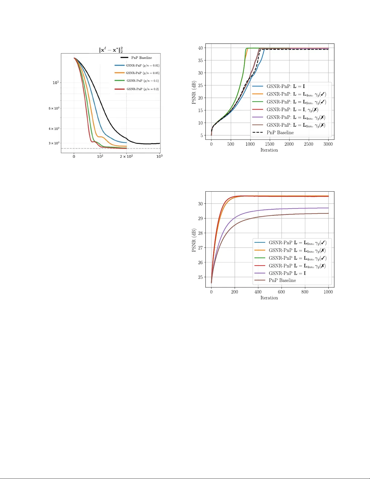
GSNR: Graph Smooth Null-Space Repr esentation f or In verse Pr oblems Romario Gualdr ´ on-Hurtado * , Roman Jacome * , Rafael S. Suarez, Henry Ar guello Uni versidad Industrial de Santander , Colombia, 680002 { yesid2238324,rajaccar,rafael2269082 } @correo.uis.edu.co , henarfu@uis.edu.co Abstract In verse pr oblems in imaging ar e ill-posed, leading to in- ﬁnitely many solutions consistent with the measur ements due to the non-trivial null-space of the sensing matrix. Common imag e priors pr omote solutions on the gener al image manifold, such as sparsity , smoothness, or score function. However , as these priors do not constrain the null-space component, the y can bias the r econstruction. Thus, we aim to incorporate meaningful null-space infor- mation in the r econstruction frame work. Inspir ed by smooth image r epr esentation on graphs, we pr opose Gr aph-Smooth Null-Space Repr esentation (GSNR), a mec hanism that im- poses structur e only into the in visible component. P ar - ticularly , given a graph Laplacian, we construct a null- r estricted Laplacian that encodes similarity between neigh- boring pixels in the null-space signal, and we design a low- dimensional pr ojection matrix fr om the p -smoothest spec- tral gr aph modes (lowest gr aph fr equencies). This approac h has str ong theor etical and practical implications: i) im- pr oved con ver gence via a null-only graph r egularizer , ii) better coverag e, how much null-space variance is captur ed by p modes, and iii) high pr edictability , how well these modes can be inferr ed fr om the measur ements. GSNR is incorporated into well-known in verse pr oblem solvers, e .g., PnP , DIP , and diffusion solvers, in four scenarios: ima ge deblurring, compr essed sensing, demosaicing, and imag e super-r esolution, pr oviding consistent impr ovement of up to 4.3 dB over baseline formulations and up to 1 dB compar ed with end-to-end learned models in terms of PSNR. 1. Introduction Recov ering an image from a limited number of noisy mea- surements requires estimating a solution to an undetermined in v erse problem, which is of the form y = Hx ∗ + ω , ω ∼ N ( 0 , σ 2 I ) . (1) where y ∈ R m denotes the measurement vector , x ∗ ∈ R n is the unkno wn tar get image, H ∈ R m × n is the sensing matrix with m ≤ n , and ω models additiv e Gaussian noise. This formulation is used in a broad range of imaging tasks * Equal contribution. by using a proper structure of H . Compressed sensing (CS) tasks employ dense sensing matrices [ 5 ]. Image restora- tion problems, such as deblurring [ 53 ], inpainting [ 51 ], and super-resolution [ 46 ], are modeled by structured T oeplitz or block-diagonal matrices. In medical imaging, modalities like magnetic resonance imaging (MRI) [ 26 ] and computed tomography (CT) [ 2 ] use structured physics-based opera- tors (e.g., undersampled Fourier or Radon transforms). The formulation in ( 1 ) becomes ill-posed due to matrix instabil- ity and/or the undersampling scheme. Therefore, incorpo- rating prior knowledge or regularization is essential to pro- mote reconstructions that are consistent with the expected structure of x ∗ [ 4 ]. The estimation of x ∗ is commonly formulated as a variational problem that combines a data- ﬁdelity term and a regularization term: b x = arg min ˜ x 1 2 ∥ H˜ x − y ∥ 2 2 | {z } data ﬁdelity: g ( ˜ x ) + λ f ( ˜ x ) | {z } prior (2) where g ( ˜ x ) enforces consistency with the measurements and f ( ˜ x ) incorporates prior kno wledge about the struc- ture of x ∗ . Recent advances have introduced data-driv en regularizers for f ( ˜ x ) , most notably Plug-and-Play (PnP) [ 6 , 20 , 48 , 52 ] and Regularization by Denoising (RED) [ 9 , 34 , 35 ], which hav e achie v ed remarkable success across a wide range of imaging tasks [ 20 ] by implicitly promot- ing solutions within the training image dataset manifold i.e., well-trained denoiser learns the data score-function [ 27 ]. PnP and RED use learned denoisers, allo wing the inte- gration of powerful deep restoration networks within algo- rithms [ 27 , 44 ]. Despite their versatility and success, these priors operate in the image domain and do not explicitly ex- ploit the structure of H , including its null-space (NS). Only a portion of x ∗ is observ able through H . The range-null- space decomposition (RNSD) states that any x ∈ R n vector is decomposed as x = x r + x n , where x r = P r x de- notes the component lying in the range space of H , with P r = H † H , and x n = P n x denotes the component lying in its NS, with the NS projector P n = I − H † H . x n is in visible to H because it belongs its NS, deﬁned as Null( H ) = { x ∈ R n : Hx = 0 } = { x : x ⊥ h j , ∀ j ∈ { 1 , . . . , m }} , where h j ∈ R n is the j -th row of H . This interpretation has inspired approaches that explicitly exploit Null( H ) . Null-Space Networks (NSN) [ 41 ] and Deep Decomposi- tion [ 7 ] operate across the entire Null( H ) , treating all in- visible directions as equally relev ant, neglecting the fact that natural, perceptually plausible images occupy only a low-dimensional manifold within that space [ 17 ]. T o ad- dress this gap, the recent Nonlinear Projections of the Null- Space (NPN) frame work [ 17 ] introduces a learnable low- dimensional NS projection matrix S ∈ R p × n , with p ≤ ( n − m ) . S is designed depending on the in verse prob- lem, making its ro ws orthogonal to H , then S is opti- mized jointly a NS component predictor G( y ) ≡ Sx ∗ to adapt the span( S ) into a subspace of Null( H ) . During reconstruction, NPN penalizes deviations ∥ G( y ) − S ˜ x ∥ 2 2 . Howe ver , natural images occupy a low-dimensional, struc- tured subset inside Null( H ) , so blindly learning an arbitrary span( S ⊤ ) ⊂ Null( H ) can waste capacity and induce bias. In this work, we present a principled framework that pro- vides a new representation of the NS, enabling the optimal selection of informative NS directions. T o address this is- sue, we took into account two main optimality criteria: Coverage: How much of the null-space of H is r epr e- sented with the pr ojection matrix S . Predictability: How easily can the projections Sx be estimated fr om the measurements y only . Inspired by the graph (smooth) representation of im- ages [ 28 , 29 ], we introduce Graph-Smooth Null-Space Rep- resentation (GSNR) to overcome the shortcomings of NS representation and prediction. Different from the well- studied graph-structure preserving approach in imaging in- verse problems [ 19 , 28 ] that promotes smoothness over the image x , our approach is the ﬁrst to endow the NS compo- nent x n with a graph structure, deﬁned through a sparse, positiv e semideﬁnite graph Laplacian L ⪰ 0 , such as 4/8-nearest-neighbor (NN) image grid whose edge weights encode local pixel similarity . W e form the null-r estricted Laplacian T := P n L P n on Null( H ) . V ia spectral graph theory , we construct the graph-smooth NS projection matrix S as the p -smoothest NS modes, which corresponds to the p ﬁrst graph F ourier modes. The proposed GSNR changes how we solve in v erse problems by providing ex- act structure information where the sensor is blind. By se- lecting the p -smoothest eigenmodes of the null-restricted Laplacian, our method (i) reduces hallucinations and bias by constraining only the in visible component, not the whole image; (ii) impro ves conditioning, leading to faster and more stable con v ergence across PnP , DIP , and diffusion solvers; (iii) increases data efﬁciency by capturing most null-space v ariation with small p (high coverage) and by targeting the modes that are easiest to infer from measure- ments (high predictability); and (iv) offers operational di- agnostics coverage/predictability curves that allows select- ing p and justify regularization objectively . Because it is plug-compatible with standard pipelines and agnostic to the forward operator , the approach scales across dif ferent imag- ing tasks, turning an ill-posed ambiguity into a structured, measurable, and learnable component. The proposed con- struction has the following beneﬁts: 1. Selected graph-smooth null-space components produce high coverage at low dimensionality projection, i.e., small p (Theorem 1 and Theorem 2 ). 2. Predicting the p null-space components from y using a GSNR is easier than the ones obtained with a common null-space basis (Proposition 1 ). 3. Predicted graph null-space components can be incorpo- rated via regularization into solvers such as PnP , Deep Image Prior , and Dif fusion Models. 2. Related W ork V ariational and learned priors. A common scheme to solve ( 2 ) is proximal gradient descent (PGD) [ 30 ]. Re- cently , PnP [ 20 ] and RED [ 35 ] methods hav e replaced the proximal operator of f ( ˜ x ) with learned denoisers, enabling the incorporation of data-driv en priors without requiring an explicit analytic form [ 17 ]. Although these frameworks achiev e state-of-the-art performance, they lea ve Null( H ) largely unconstrained; denoisers may freely modify com- ponents that are in visible to the sensing operator . Nonlinear Pr ojections of the Null-Space (NPN). T o e xplicitly regularize image unobserved components, [ 17 ] introduced a task-speciﬁc lo w-dimensional projection within Null( H ) , enforcing consistency between learned NS predictions and reconstructions. Building on this principle, we propose GSNR, which incorporates graph-smoothness analysis to guide the selection of a structured null-subspace. Our design ensures that the learned projection aligns with the intrinsic geometry of the data, yielding NS components that are both predictable from the measurements and con- sistent with the graph-induced smoothness prior . Graph theory in imaging in verse pr oblems . V aria- tional regularization methods address inv erse problems by imposing smoothness or sparsity priors that constrain the solution space. T otal v ariation [ 38 ] enforces pixel-wise smoothness, whereas wavelet-based sparsity priors [ 13 ] promote sparse representations of images in the transform domain via soft-thresholding. Although these priors im- prov e stability , they are typically limited to local structures and often oversmooth ﬁne textures or complex geometries. T o better capture local dependencies, graph-based and non- local regularization methods have been reintroduced. [ 32 ] proposed an adaptive nonlocal regularization framework that jointly estimates the image and the graph that encodes patch similarities. Howe v er , like classical priors, this frame- work operates solely on the reconstruction and doesn’t con- strain the image component lying in Null( H ) . 3. Graph-Smooth Null-Space Representation 3.1. Preliminaries: Graphs Graphs provide a geometric representation of data, where vertices correspond to data elements (e.g., pixels or image patches) and weighted edges encode pairwise similarities between them [ 42 ]. Signals deﬁned on weighted undirected graphs are mathematically denoted by G = ( V , E , W ) , where V is the vertex set with |V | = n , E ⊆ V × V is the edge set, and W ∈ R n × n is the symmetric weighted adjacency matrix with W ij > 0 if ( i, j ) ∈ E and W ij = 0 otherwise. The unnormalized graph Laplacian is L = D − W , ( Lx ) i = X j W ij  x i − x j  , (3) where the diagonal degree matrix D = diag( d 1 , . . . , d n ) accomplishes d i = P j W ij . Its Dirichlet energy is x ⊤ Lx = 1 2 X i,j W ij  x i − x j  2 , (4) which penalizes discrepancies across edges with large weights. F or symmetric W , L is real symmetric pos- itiv e semideﬁnite (SPSD) with eigenpairs { ( λ ℓ , v ℓ ) } n − 1 ℓ =0 , 0 = λ 0 ≤ λ 1 ≤ · · · , v 0 ∝ 1 on connected graphs. Eigen- vectors with small λ ℓ vary slowly across high-weight edges, motiv ating the interpretation of λ as a graph frequency . For the usage of L , we focus on two graph topologies [ 29 ]: 1. 4NN: This promotes piecewise smoothness aligned with the coordinate axes and attenuates horizontal/ver - tical ﬂuctuations, yielding an anisotropic (axis-biased) smoothing ef fect. Here, E 4 = { ( i, j ) : ∥ p i − p j ∥ 1 = 1 } , W ij = 1 ( i,j ) ∈E 4 , with p i ∈ Z 2 pixel coordinates. 2. 8NN: This reduces orientation bias and more closely approximates an isotropic Laplace operator , promoting rotation-in v ariant piecewise smoothness and suppressing ﬂuctuations uniformly across directions. Here, E 8 = { ( i, j ) : ∥ p i − p j ∥ ∞ = 1 } , W ij = w o 1 ∥·∥ 2 =1 + w d 1 ∥·∥ 2 = √ 2 , where w d = w o / √ 2 . Nev ertheless, we extend the analysis of the proposed ap- proach to other topologies in Supp. A4.1 . 3.2. Graph-smooth null modes W e study smoothness within the NS by restricting the Laplacian to T = P n LP n , (5) the reason for using the null-graph operator T ∈ R n × n stems from the need to pay attention to certain geometric properties of the image’ s NS, which are extracted by L . Let Tx = P n LP n x = P n Lx n , where Lx n extracts, ar- eas of greatest difference in the NS, and then re-project it to the NS with P n , thus ensuring that this operation re- sults in a projection from the NS. In Fig. 1 , from left to right, we show the ground-truth x ∗ , back-projection H ⊤ y , true null component P n x ∗ , and two graph NS projections P n L 8 nn P n x ∗ and P n L 4 nn P n x ∗ , for super-resolution (SR). Figure 1. For image SR task with S RF = 4 , n = 3 · 128 2 , we show ground-truth, adjoint reconstruction, NS projection, projec- tion onto graph-smooth NS with L 4 nn and L 8 nn . The map P n x ∗ isolates signal content in visible to the sen- sor , while P n LP n x ∗ highlights where Lx n falls into the NS. These graph projections highlight the smoothest blind signal components, e.g., textures near edges. Then, by applying eigen v alue decomposition, we see that T = V diag ( µ 1 , . . . , µ n ) V ⊤ is SPSD, with 0 ≤ µ 1 ≤ · · · ≤ µ n , where V ∈ R n × n is orthogonal. Note that V diagonalizes T , so its columns { v i } are the graph-F ourier modes within Null( H ) . If µ i is smaller, then a smoother graph-mode is selected. V has the following properties: i) V has orthonormal columns v i ∈ Null( H ) , µ i -ordered. ii) These { v i } are graph-smooth null modes probing x . The graph-smooth NS projector S with p rows is obtained by taking the ﬁrst p columns of V : S = V ⊤ p z }| { V [: , 1 : p ] ⊤ = [ v 1 , . . . , v p ] ⊤ ∈ R p × n . (6) Note that S keeps only the p -smoothest null directions and Sx expresses the NS part of x in an orthonormal basis sorted by increasing graph frequency . Particularly , based on RNSD: Sx = S  P r + P n  x = SP r x + SP n x , since rows of S lie in Null( H ) , hence SP r = 0 , leading to Sx = 0 + SP n x = V ⊤ p P n x =   ⟨ v 1 , x n ⟩ . . . ⟨ v p , x n ⟩   . Here { v i } p i =1 are the p Laplacian-smoothest orthonormal null modes; thus Sx collects the coefﬁcients of x along these p directions. 3.3. Learning lo w-dimensional GSNR W e train the GSNR predictor G follo wing: G ∗ = min G E  ∥ G( y ) − Sx ∗ ∥ 2 2  . (7) Here, we aim to predict the low-dimensional GSNR using the neural network G . Subsequently , the theoretical foun- dations will be laid that greater predictability will guarantee better con v ergence in the task. 3.4. Reconstruction objective Thus, we incorporate our method as min ˜ x g ( ˜ x ) + λ f ( ˜ x ) + γ ∥ G ∗ ( y ) − S ˜ x ∥ 2 2 + γ g 2 ϕ ( ˜ x ) z }| { ˜ x ⊤ T˜ x , (8) which includes the learned GSNR term, plus a graph regu- larizer acting only on the null component of the reconstruc- tion, weighted by γ and γ g , respectively . This retains com- patibility with proximal/PnP/DM solvers. 4. Theory and Analysis W e develop a theoretical analysis on GSNR based on null-r estricted spectral formulation that turns GSNR de- sign/performance prediction into ordered-eigenv alue crite- ria on T for optimal subspace selection, obtaining a princi- pled eigen-ordering and criteria used to choose S , p, L . The theoretical results are summarized as: Covera ge : the ﬁrst p eigenmodes of T provide an opti- mal graph-smooth representation of Null( H ) , by cov- ering a high null-space spectrum energy with p ≪ n − m . Minimax optimality : the same GSNR basis is worst- case optimal o ver a graph-energy ellipsoid in Null( H ) , giving a principled ordering of null directions Pr edictability : via block-precision/Schur-complement analysis, we show that GSNR has a higher per-mode recov erability from measurements y than plain null- space projections. Con ver gence : the effect of the graph regularizer pro- vides better conditioning and con vergence properties based on ﬁxed-point analysis. 4.1. Null-space coverage Before dev eloping the formal analysis on the cov erage properties of the NS projections, we validate the represen- tation performance of three settings: i) L = I , ii) L 4 nn , and iii) L 8 nn . Note that the ﬁrst setting is equiv alent to just tak- ing the NS basis. In Fig. 2 (a), each ro w shows projections ( x = ( H ⊤ H + S ⊤ S ) x ∗ ) as the dimension of the null–space subspace increases, p ∈ { 153 , 1536 , 4608 , 9216 , 15360 } , for three graph choices in the design of S : (top, orange) L = I ; (middle, green) grid L 8 nn ; (bottom, blue) grid L 4 nn . For small p , the grid Laplacians already yield visually plau- sible faces, while L = I still produces noisy , poorly struc- tured estimates. The number printed above each image is the MSE of the representation. The plot at the bottom shows the MSE for all values of p = { 1 , . . . , n − m } , sho wing that the graph-null-space projections provide better signal representation with smaller p than just the NS basis. In gen- eral, to measure the amount of energy from the NS that the low-dimensional operator S can capture, we use the spectral cov erage deﬁned as: C ( p ) = tr  S Co v( x n ) S ⊤  tr (Co v( x n )) ∈ [0 , 1] , (9) where Cov( x ) is the cov ariance matrix of x . V iew the Laplacian eigen v ectors as a graph–Fourier basis: the ﬁrst modes are smooth, low “graph–frequency” patterns, while later modes are increasingly oscillatory [ 29 , 42 ]. The C ( p ) indicates what fraction of the total NS variance lies in the span of the ﬁrst p graph–Fourier modes retained by S , sim- ilarly as explained variance in PCA [ 18 ]. Intuitiv ely , if the signal is graph–smooth, most variability concentrates in low Figure 2. Cov erage and spectral analysis for SR task. (a) x ∗ = H ⊤ Hx ∗ + S ⊤ Sx ∗ for S given by ( 6 ) using L = I (orange), L = L 4 nn (green) and L = L 8 nn (blue) for dif ferent values of p . (b) RNSD representation error , varying p . (c) V ariation of T normalized eigen v alues with respect to their index. frequencies, so coverage climbs rapidly with small p ; if not, cov erage gro ws more slowly , like in PCA. A4.2 shows cov- erage results and eigen v alue analysis that v alidate the use- fulness of graph Laplacians, rather than a learnable matrix. Mathematical insights for the selection of the appropriate p value depending on the co v erage are gi ven in A5 . Deﬁnition 1 (Gaussian Markov Random Field [ 39 ]) A GMRF on the graph G = ( V , E ) is a zer o-mean Gaussian vector x ∈ R n with pr ecision matrix Q = Σ − 1 ∈ R n × n , with Σ = Cov( x ) , is sparse and encodes the conditional independence of the graph p ( x ) ∝ exp  − 1 2 x ⊤ Qx  , Q i,j = 0 ← → ( i, j ) / ∈ E , wher e smoothness is r equir ed in neighboring pixels, we de- ﬁne the pr ecision matrix Q = α L + ϵ I with α > 0 , ϵ > 0 . Under this setting, we deriv e the following guarantee on im- prov ed NS cov erage. Theorem 1 (Co verage f or graph-smooth null-space) Consider the construction of T in ( 5 ) . The covariance of the NS, Co v( x n ) is a spectral function of T , i.e., Co v( x n ) = V diag( λ 1 , . . . , λ n ) V ⊤ , where λ i = 1 αµ i + ϵ , λ 1 ≥ λ 2 · · · ≥ λ n . W ith the construction of S in ( 6 ) , the covera ge of the NS using GMRF with a Laplacian matrix L as C L ( p ) and the covera ge when L = I is denoted C I ( p ) , satisﬁes for every p = 1 , . . . , n − m . C L ( p ) ≥ C I ( p ) . The proof can be found in Supp. A1 . W e illustrate this effect in Fig. 2 (b)-(c). In 2 (b), the rep- resentation error of the RNSD decreases more rapidly when using L 8 nn and L 4 nn compared to I . In 2 (c), the eigen- value spectra of T rev eal that, unlike the ﬂat spectrum of the pure NS projector P n , graph Laplacians exhibit smoothly increasing eigenv alues. From Theorem 1 , a ﬂat spectrum ( µ i = 1 for all i as with L = I ) yields C I ( p ) = p/q , so cov- erage grows only linearly with p , whereas Laplacians with increasing { µ i } achiev e faster co v erage gro wth. Our second theoretical result is a minimax optimality on the NS coverage by the NS scheme. First, deﬁne the feasible set of NS components M τ :=  x n ∈ Null( H ) : x ⊤ n L x n ≤ τ  Theorem 2 (Minimax optimality) Let V p = span { v 1 , . . . , v p } and P V p be its projector . Then, among all p -dimensional V ⊂ Null( H ) , pr ovided µ p +1 > 0 , min dim( V )= p sup x n ∈M τ ∥ ( I − P V ) x n ∥ 2 2 = sup x n ∈M τ ∥ ( I − P V p ) x n ∥ 2 2 = τ µ p +1 . The proof of this theorem is in Supp. A2 . Remark 1 Selecting S so that its r ows ar e { v ⊤ 1 , . . . , v ⊤ p } is pro vably optimal for covering the NS under the gr aph ener gy x ⊤ Tx . As p gr ows, the guaranteed worst-case er- r or decays with 1 /µ p +1 , which is fast for gr aph Laplacians (wher e many µ j ar e small). W ith L = I one gets T = P n (ﬂat spectrum), hence µ p +1 = 1 and no impr ovement in the bound, explaining why geometry-fr ee designs cannot cover the NS efﬁciently . 4.2. Null-space projections pr edictability It is also important to quantify the predictability level of the NS projections Sx ∗ from the acquired measurements y . W e dev elop a statistical coupling analysis via linear estimation. Proposition 1 (P er–mode pr edictability bound) Let x ∈ R n be zer o–mean Gaussian with covariance C and pr eci- sion Q = C − 1 . Let H ∈ R m × n and denote the orthogonal pr ojectors onto R := Range( H ⊤ ) and N := Null( H ) by P r and P n , r espectively . Block Q and C with respect to the decomposition R n = R ⊕ N : Q =  Q rr Q rn Q nr Q nn  , C =  C rr C rn C nr C nn  . Assume Q nn ≻ 0 on N and let { v j } be an orthonor - mal eigenbasis of Q nn with Q nn v j = µ j v j and µ j > 0 . Deﬁne the j -th null coef ﬁcient a j := v ⊤ j x n wher e x n := P n x . Consider measurements fr om ( 1 ) and denote C y := HC rr H ⊤ + σ 2 I m . Then the population R 2 of the optimal linear pr edictor of a j fr om y satisﬁes ρ 2 j := Co v( a j , y ) ⊤ C − 1 y Co v( y , a j ) V ar( a j ) ≤ c j c j + µ j , c j := v ⊤ j  Q rn C rr Q nr  v j . Figure 3. Per-mode predictability for each case when L ∈ { I , L 8 nn , L 4 nn } for SR case with S RF = 4 with n = 64 2 . The proof of this proposition is found in Supp. A3 . Remark 2 If the prior is a GMRF with pr ecision Q = α L + ε I on L , then Q nn = α T + ε P n with T := P n LP n , and one can take { v j } as the T –eigenmodes (graph-smooth null modes). The bound becomes ρ 2 j ≤ c j c j + α λ j ( T ) + ε , c j = v ⊤ j  Q rn C rr Q nr  v j , with Q rn = α L rn . Thus smoother null modes (small λ j ( T ) ) ar e more predictable . Now , if L = I (isotr opic prior), then Q = γ I and Q rn = P r Q P n = 0 , so c j = 0 and ρ 2 j ≤ 0 for all j : ther e is no statistical coupling between R and N . T o ev aluate the de veloped theory , Fig. 3 , the empirical per–mode predictability ρ 2 j (one dot per eigenmode), for three choices of L ∈ { L 8 nn , L 4 nn , I } , where L = I has same index ordering across panels. From indices [0 , m − 1] , the predictability is high for all settings, since they corre- spond to the eigenpairs related to the Range space, thus, the predictability is high. The observ ations are: (i) for L = I , the spectrum is constant over the NS and then drops to 0 outside of it, while both grid Laplacians exhibit a smooth, monotone growth of µ j ; (ii) correspondingly , with grid Laplacians, a long tail of modes has non-zero predictability , ( ρ 2 j spread over a wide index range), whereas with L = I only a small initial block of modes sho ws an y predictability , and the rest are essentially 0 . Note also that L 4 nn has higher predictability than L 8 nn in more eigenmodes, follo wing the fast increase eigen value distrib ution Fig 2 (c). Note that this analysis was using a linear estimation framew ork, harnessing the NS GMRF prior . In practice, the statistical coupling can also be achiev ed with the super - vised learning of the predictor G in Eq. ( 7 ), but the trend of GS prior holds on this setting. T o e v aluate the predictability of the learned predictor , we used R 2 ( p ) ≜ 1 − E h ∥ G ∗ ( y ) − Sx ∗ ∥ 2 2 i E h ∥ Sx ∗ ∥ 2 2 i . (10) a) b) Figure 4. a) Coverage and b) Predictability vs. p for CS with CIF AR-10 dataset. In this case, m/n = 0 . 1 and p = 1 · · · n − m . 4.3. Graph-based regularizer Consider the PnP–PGD iteration solving the optimization problem ( 8 ) without the term ∥ G ∗ ( y ) − Sx ∥ (for more de- tailed analysis of this term, see [ 17 , Theorem 1]), x k +1 = D σ  x k − α  ∇ g ( x k ) + γ g ∇ ϕ ( x k )   (11) = D σ  x k − α  H ⊤ ( Hx k − y ) + γ g Tx k   , (12) where D σ is a bounded denoiser with ∥ D σ ( u ) − D σ ( v ) ∥ ≤ √ 1 + δ ∥ u − v ∥ (as in [ 17 , Assumption 2]), since ∇ ϕ ( x k ) = T ⊤ x k = Tx k . Let λ min > 0 and λ max be the extreme eigen values of A γ g = H ⊤ H + γ g T on span(Range( H ⊤ ) ∪ Null( H )) = R n . Then for any step size α ∈ (0 , 2 /λ max ) , ∥ x k +1 − x ∗ ∥ ≤ (1 + δ ) ∥ I − α A γ g ∥ 2 ∥ x k − x ∗ ∥ (13) ≤ ρ ∥ x k − x ∗ ∥ , (14) where ρ = (1 + δ ) max { 1 − αλ min , α λ max − 1 } . In par- ticular , if ρ < 1 , The iteration is a contraction and con- ver ges linearly to a ﬁxed point. The optimal α (for this lin- ear bound) is α ∗ = 2 λ min + λ max with rate ρ ∗ = (1 + δ ) κ − 1 κ +1 , κ = λ max λ min . Compared with the baseline ( γ g = 0 ), adding γ g T : (i) makes A γ g ≻ 0 ev en on Null( H ) , guaranteeing uniqueness of the quadratic subproblem, and (ii) r educes the condition number κ because T acts precisely on direc- tions where H ⊤ H is small, improving con vergence and ρ ∗ . 5. Experiments T o validate the proposed approach, we implemented it in PyT orch [ 31 ] and used the DeepIn v erse library [ 43 ] to benchmark dif ferent solvers, as detailed below . Since our work does not propose a speciﬁc network G , we validate the approach using a U-Net model [ 37 ] with a four-le v el 2D encoder–decoder architecture: the encoder applies double con v olution blocks with C, 2 C , 4 C, and 8 C channels (with C = 64 ) and 2 × 2 max-pooling, while the decoder uses nearest-neighbor upsampling with skip connections, reﬁn- ing features back to C channels before a ﬁnal 1 × 1 con vo- lution produces the output. The network is optimized using the Adam optimizer [ 21 ] with a learning rate of 10 − 3 for 50 epochs. For all experiments, we used a noise variance σ 2 = 0 . 05 . Code at 1 . W e consider the inv erse problems: 1 github .com/yromariogh/GSNR Compressed Sensing (CS): H ∈ {− 1 , 1 } m × n are the ﬁrst 10% ro ws of a Hadamard matrix A ∈ {− 1 , 1 } n × n [ 5 ]. W e validate with CIF AR-10 [ 23 ] and CelebA [ 25 ] datasets. Super -Resolution (SR): W e set n = 3 · 128 2 and use an SR factor (SRF) of 4, i.e., m = 3 · 32 2 . W e validate on the CelebA dataset [ 25 ], using 10000 training images resized to 128 × 128 . W e also sho w results for the Synthetic Aperture Radar (SAR) image dataset [ 11 ]. Demosaicing: W e used the CelebA dataset, resized to 64 × 64 , and the Bayer ﬁlter [ 3 ] acquisition pattern. Deblurring: W e set n = 64 2 · 3 and used a 2-D Gaus- sian kernel with a bandwidth σ k = 1 . W e validated our experiments on the CelebA [ 25 ] dataset and the Places365 [ 54 ] dataset, both resized to 64 × 64 , using 10000 images for training and a batch size of 32. For all of these imaging tasks, we construct the null- restricted Laplacian T and the matrix S , leveraging prop- erties of H . Details on the computation of these matrices in A5 . W e provide comprehensiv e ablations of GSNR in A6 . 5.1. Predictability and Co verage The coverage deﬁnition in ( 9 ), has a general expression for the cov ariance matrix computation. In practice, we com- puted as follows. Giv en centered images x i and their null projections x n,i = P n ( x i − ¯ x ) , where ¯ x = 1 N P N i =1 x i and the NS cov ariance Cov( x n ) = 1 N P N i =1 x n,i x ⊤ n,i . Fig. 4 shows the results in terms of (a) Coverage and (b) Pre- dictability in CS for different operators S , under the same acquisition matrix H . W e used the N = 10000 image of the CIF AR-10 dataset. In this case, NPN ( L = I ) is ob- tained following [ 17 , Eq. 3], and GSNR uses L = L 8 nn . Note that here we take the ﬁrst p rows of each S . Supp. A9 shows additional results for CS. A7 sho ws the cov erage curves for the SR task. 5.2. Diffusion Solvers W e used two diffusion model (DM) solvers, DPS [ 8 ] and DiffPIR [ 55 ]. See Supp. A8 for more details on the adap- tation of these models with the proposed approach. Fig. 5 compares DPS and DiffPIR with and without the proposed GSNR term. In all cases, the baseline DM already pro- duces plausible faces, but it often leaves residual blur and aliasing around high–frequency structures such as hair , eye- brows, and facial contours. When we replace the generic NS basis by the GSNR, the reconstructions become visibly sharper and more faithful to the ground truth: edges around the jawline and nose are better deﬁned, textures are less washed out, and blocky artifacts from the low-resolution observation y are further suppressed. These qualitative im- prov ements are consistent with the quantitativ e SSIM/P- SNR numbers printed in each panel: the gains over the baseline DiffPIR/DPS are modest in dB but systematic (e.g., 30 . 19 → 30 . 31 ; 30 . 19 → 30 . 48 ), indicating that the GSNR term helps the diffusion prior resolve NS ambiguities rather than hallucinating arbitrary details. In other words, the DM Figure 5. Results of DM-based solv ers (DPS [ 8 ] & DiffPIR [ 55 ]) for Baseline, NPN [ 17 ], and GSNR with L 4nn and L 8nn . Here, p = 0 . 1 n . T able 1. Quantitativ e comparison on the super-resolution and de- mosaicing tasks (higher is better) using the CelebA test set. For each task, the best result and second-best results. Method T ask Super-Resolution Demosaicing PnP [ 20 ] 27.37 39.35 NPN [ 17 ] 29.21 39.77 DDN-Cascade [ 7 ] 28.92 37.83 DDN-Independent [ 7 ] 28.81 38.92 DNSN [ 41 ] 26.52 39.33 Unrolling [ 50 ] 28.97 38.82 GSNR-PnP w . L 8 nn 29.38 39.88 GSNR-PnP w . L 4 nn 29.42 39.89 still provides the powerful image prior, but GSNR steers it along graph-smooth NS directions that are predictable from y and compatible with the forward model, yielding more accurate and stable reconstructions. Supp. A8 shows the integration of GSNR in latent-space DMs [ 15 ]. 5.3. Comparison with End-to-End Methods T able 1 reports PSNR on SR and demosaicing, comparing classical PnP , the proposed GSNR-PnP variants, NPN, and sev eral strong deep-learning baselines. Across both tasks, GSNR-PnP with graph Laplacians L 4 nn and L 8 nn achiev es the best performance. For SR, GSNR-PnP yields roughly a 2 dB gain over vanilla PGD-PnP and a clear margin over both NPN (with L = I ) and task-speciﬁc unrolled/cascade architectures. For demosaicing, the problem is less ill- posed, so the absolute gains are smaller, but GSNR-PnP still provides a consistent improvement o ver PGD-PnP , NPN, and the deep baselines. Overall, these results show that injecting graph-smooth NS structure into a standard PnP solver consistently improves upon (i) geometry-free Pn- P/NPN baselines and (ii) specialized deep unrolled or cas- cade architectures, with particularly strong beneﬁts on the most underdetermined SR task. In A10 and A11 , we show additional results for Demosaicking and SR, respectiv ely . T able 2. Final PSNR (dB) for deblurring ( σ k = 1 ) with n = 64 2 · 3 and p = 0 . 8 · n . W e report results on Places365 [ 11 ] and CelebA [ 25 ] test sets using Lip-DnCNN [ 40 ] and a wa velet denoiser [ 12 ]. For each column, best and second-best results. Method γ g Places365 CelebA Lip-DnCNN W avelet Lip-DnCNN W av elet Baseline (PGD-PnP) – 31.58 30.78 35.26 33.64 NPN [ 17 ] – 33.22 33.17 37.86 37.68 GSNR w . L 8 nn ✘ 33.60 33.59 38.18 37.99 GSNR w . L 8 nn ✓ 33.60 33.59 38.18 37.99 5.4. Plug-and-Play W e used the PGD-PnP [ 16 , 20 ], but GSNR can be easily adapted to other formulations, such as ADMM [ 6 ] or HQS [ 33 ]. W e used three denoisers: DnCNN with Lipchitz train- ing (Lip-DnCNN) [ 40 ], DRUNet [ 52 ], W avelet denoiser (Daubechies 8 with 4 levels) using soft-thresholding prox- imal [ 12 ]. For improving stability and performance of the PGD-PnP , we include the equiv ariant denoising technique [ 45 ] with two random 90 rotations and two reﬂections. Deblurring : T able 2 reports the ﬁnal PSNR for deblur- ring on Places365 and CelebA under different graph vari- ants and denoisers. In all settings, both NPN and GSNR substantially improv e o ver the baseline PGD-PnP solver: on CelebA, the gain is on the order of +2 dB for both Lip- DnCNN and the w av elet denoiser , and on Places365, the gain is around +1 . 5 – 2 dB. The GSNR v ariant with L 8 nn provides a small but consistent improvement over NPN on both datasets and for both denoisers, indicating that inject- ing NS structure into the NS helps the solver recov er sharper details without overﬁtting. Interestingly , turning the addi- tional graph penalty on or off ( γ g ✓ vs. ✘ ) has a negligi- ble effect on the ﬁnal PSNR in this experiment, suggesting that the learned GSNR already captures most of the useful graph structure for deblurring. Figure 6 shows the deblur- ring con ver gence beha viour with the DnCNN denoiser . The baseline PnP-PGD curve increases steadily but saturates at a lower PSNR plateau. In contrast, both GSNR variants (with γ g = 0 and γ g = 0 . 1 ) con ver ge to a noticeably higher ﬁnal PSNR, conﬁrming that the graph-smooth null-space repre- Figure 6. Deblurring con ver gence curves for PnP-PGD baseline using Lip-DnCNN and GSNR variants with L 8 nn with and with- out the null-restricted Laplacian regularization. sentation impro ves the ﬁxed point of the algorithm. The e x- plicit null-only graph penalty ( γ g = 0 . 1 ) mainly affects the transient regime: it accelerates conv er gence in the ﬁrst few hundred iterations, reaching near-peak PSNR signiﬁcantly earlier than GSNR with γ g = 0 (aligned with the theoreti- cal analysis conducted in Sec. 4.3 ), while all three methods ev entually stabilize. Additional visual results in A12 . SR : Fig. 7 shows an SR example for dif ferent graph de- signs and denoisers. Columns correspond to the choice of Laplacian L or to the baseline PnP without GSNR, while rows correspond to different denoisers. In all three ro ws, moving from the baseline and L = I columns to the graph- based L 4nn and L 8nn columns produces visibly sharper details: facial contours are crisper, hair strands are bet- ter resolved, and blocky artifacts inherited from the lo w- resolution backprojection H ⊤ y are reduced. The improve- ments are most pronounced for the DnCNN and DRUNet denoisers. Still, they are also clearly present for the simpler W avelet denoiser , indicating that the beneﬁt comes from the GSNR itself rather than from the denoiser . Among the graph designs, L 8nn yields the visually clearest reconstruc- tion, suggesting that richer graph connectivity enables the solver to exploit structure in the null space rather than hallu- cinating high-frequency content. Results with Deep Image Prior [ 49 ] and SAR images in SR can be found in A11 . 6. Discussion W e demonstrate that GSNR is a versatile approach for a broad range of in verse problems, data modalities, and neu- ral networks ( A14 ). Nev ertheless, the method requires pre- cise knowledge of the sensing matrix, which is unav ail- able in some applications, e.g., real-world image deblurring. In A15 , we provide analysis on the effect of uncertainty in the sensing operator, where a performance drop is evi- dent, but the impro v ement compared with the baseline algo- rithm is maintained. F ollo w-up ideas will harness the null- space construction under sensing matrix uncertainty for cal- ibrated null-space regularization functions. Another aspect Figure 7. Results of PnP , NPN, and GSNR varying L and denois- ers. Best results for each denoiser are in bold. Here, p = 0 . 1 n . of GSNR is the requirement to perform EVD on the null- restricted Laplacian T , which, at lar ge image scales, neces- sitates substantial computational resources. Howe ver , this computation is performed ofﬂine once per ( H , L , n, p ) , and reused for learning the network G and the reconstruction step. In A13 , we provide a detailed runtime analysis of the approach. Additionally , our approach is designed for lin- ear in verse problems; the adaptation for nonlinear in verse problems, e.g., phase retrie val, requires careful modeling of the in vertibility properties of the sensing operator and its input-dependent ambiguities. In recent work [ 14 ], a gener- alization of the null-space property was de veloped for neu- ral networks (non-linear functions), opening new frontiers for learning optimal null-space components. 7. Conclusion and Future Outlook W e introduced GSNR: Graph-Smooth Null-Space Repr e- sentation , which equips an inv erse problem solver not only with what the measurements constrain, b ut also with how to use the degrees of freedom that the sensor never sees (null- space). Instead of regularizing the full image, GSNR b uilds a lo w-dimensional basis for Null( H ) aligned with graph smoothness via the null-restricted Laplacian T = P n LP n , and can optionally add a null-only graph penalty at infer- ence. Theoretically , the smoothest T -modes are minimax- optimal for null-space components, and under a GMRF prior , they prov ably capture more null-space variance than geometry-free choices while enjoying stronger statistical coupling to the measurements. In practice, this yields bet- ter coverage of plausible solutions, higher predictability of null-space signal components, and improv ed conditioning, translating into faster and more stable conv ergence of PnP and diffusion-based solvers. Looking ahead, rather than ﬁx- ing L to a hand-crafted grid Laplacian, learning the graph structure or employing interpretable graph neural operators promises data-adaptive GSNR bases that better reﬂect se- mantic structure. Also, a more rigorous study of GSNR within generativ e solvers could pro vide a principled way to inject graph-smooth null constraints into these frame works without breaking their probabilistic interpretation. References [1] Eirikur Agustsson and Radu T imofte. Ntire 2017 challenge on single image super-resolution: Dataset and study . In The IEEE Conference on Computer V ision and P attern Recogni- tion (CVPR) W orkshops , 2017. 11 [2] Daniel Otero Baguer, Johannes Leuschner, and Maximilian Schmidt. Computed tomography reconstruction using deep image prior and learned reconstruction methods. In verse Pr oblems , 36(9):094004, 2020. 1 [3] Bryce E Bayer . Color imaging array , 1976. US Patent 3,971,065. 6 [4] Martin Benning and Martin Burger . Modern regularization methods for inv erse problems. Acta numerica , 27:1–111, 2018. 1 [5] E. J. Candes and M. B. W akin. An introduction to com- pressiv e sampling. IEEE Signal Pr ocessing Magazine , 25 (2):21–30, 2008. 1 , 6 [6] Stanley H Chan, Xiran W ang, and Omar A Elgendy . Plug- and-play admm for image restoration: Fix ed-point conv er - gence and applications. IEEE T ransactions on Computa- tional Imaging , 3(1):84–98, 2016. 1 , 7 [7] Dongdong Chen and Mike E Davies. Deep decomposition learning for in verse imaging problems. In Computer V ision– ECCV 2020: 16th Eur opean Confer ence, Glasgow , UK, Au- gust 23–28, 2020, Proceedings, P art XXVIII 16 , pages 510– 526. Springer , 2020. 2 , 7 [8] Hyungjin Chung, Jeongsol Kim, Michael Thompson Mc- cann, Marc Louis Klasky , and Jong Chul Y e. Diffusion pos- terior sampling for general noisy inv erse problems. In The Eleventh International Conference on Learning Repr esenta- tions , 2023. 6 , 7 , 1 [9] Rege v Cohen, Michael Elad, and Peyman Milanfar . Regu- larization by denoising via ﬁxed-point projection (red-pro). SIAM Journal on Imaging Sciences , 14(3):1374–1406, 2021. 1 [10] Y uning Cui, Syed W aqas Zamir , Salman Khan, Alois Knoll, Mubarak Shah, and Fahad Shahbaz Khan. Adair: Adaptiv e all-in-one image restoration via frequency mining and mod- ulation. In 13th international conference on learning rep- r esentations, ICLR 2025 , pages 57335–57356. International Conference on Learning Representations, ICLR, 2025. 11 [11] Emanuele Dalsasso, Xiangli Y ang, Lo ¨ ıc Denis, Florence T upin, and W en Y ang. Sar image despeckling by deep neural networks: From a pre-trained model to an end-to-end train- ing strategy . Remote Sensing , 12(16):2636, 2020. 6 , 7 [12] David L Donoho. De-noising by soft-thresholding. IEEE transactions on information theory , 41(3):613–627, 2002. 7 [13] David L Donoho and Iain M Johnstone. Ideal spatial adapta- tion by wavelet shrinkage. Biometrika , 81(3):425–455, 1994. 2 [14] Y amit Ehrlich, Nimrod Berman, and Assaf Shocher . Pseudo-in vertible neural networks. arXiv pr eprint arXiv:2602.06042 , 2026. 8 [15] Y utong He, Naoki Murata, Chieh-Hsin Lai, Y uhta T akida, T oshimitsu Uesaka, Dongjun Kim, W ei-Hsiang Liao, Y uki Mitsufuji, J Zico K olter , Ruslan Salakhutdinov , and Ste- fano Ermon. Manifold preserving guided diffusion. In The T welfth International Confer ence on Learning Repr esenta- tions , 2024. 7 , 1 , 8 [16] Samuel Hurault, Antonin Chambolle, Arthur Leclaire, and Nicolas Papadakis. A relaxed proximal gradient descent algorithm for conv ergent plug-and-play with proximal de- noiser . In International Confer ence on Scale Space and V ariational Methods in Computer V ision , pages 379–392. Springer , 2023. 7 [17] Roman Jacome, Romario Gualdr ´ on-Hurtado, Le ´ on Su ´ arez- Rodr ´ ıguez, and Henry Arguello. NPN: Non-Linear Projec- tions of the Null-Space for Imaging Inv erse Problems. In The Thirty-ninth Annual Confer ence on Neural Information Pr ocessing Systems , 2025. 2 , 6 , 7 , 9 , 11 [18] Ian T Jolliffe and Jorge Cadima. Principal component analy- sis: a revie w and recent developments. Philosophical trans- actions of the r oyal society A: Mathematical, Physical and Engineering Sciences , 374(2065):20150202, 2016. 4 [19] V assilis Kalofolias. How to learn a graph from smooth sig- nals. In Artiﬁcial intelligence and statistics , pages 920–929. PMLR, 2016. 2 [20] Ulugbek S. Kamilov , Charles A. Bouman, Gregery T . Buz- zard, and Brendt W ohlberg. Plug-and-play methods for inte- grating physical and learned models in computational imag- ing: Theory , algorithms, and applications. IEEE Signal Pr o- cessing Magazine , 40(1):85–97, 2023. 1 , 2 , 7 [21] Diederik P Kingma and Jimmy Ba. Adam: A method for stochastic optimization. arXiv pr eprint arXiv:1412.6980 , 2014. 6 [22] Lingshun K ong, Jiangxin Dong, Jinhui T ang, Ming-Hsuan Y ang, and Jinshan Pan. Efﬁcient visual state space model for image deblurring. In Pr oceedings of the computer vision and pattern r ecognition confer ence , pages 12710–12719, 2025. 11 [23] Alex Krizhevsky . Learning multiple layers of features from tiny images. 2009. 6 [24] Richard B Lehoucq, Danny C Sorensen, and Chao Y ang. ARP ACK users’ guide: solution of larg e-scale eigen value pr oblems with implicitly r estarted Arnoldi methods . SIAM, 1998. 4 [25] Ziwei Liu, Ping Luo, Xiaogang W ang, and Xiaoou T ang. Deep learning face attributes in the wild. In Pr oceedings of International Confer ence on Computer V ision (ICCV) , 2015. 6 , 7 [26] Michael Lustig, David L Donoho, Juan M Santos, and John M Pauly . Compressed sensing mri. IEEE signal pr o- cessing magazine , 25(2):72–82, 2008. 1 [27] Peyman Milanfar and Mauricio Delbracio. Denoising: a powerful building block for imaging, in verse problems and machine learning. Philosophical T ransactions A , 383(2299): 20240326, 2025. 1 [28] Sunil K Narang, Y ung Hsuan Chao, and Antonio Orte ga. Graph-wa velet ﬁlterbanks for edge-aware image processing. In 2012 IEEE Statistical Signal Pr ocessing W orkshop (SSP) , pages 141–144, 2012. 2 [29] Antonio Orte ga, Pascal Frossard, Jelena K ov a ˇ cevi ´ c, Jos ´ e MF Moura, and Pierre V anderghe ynst. Graph signal processing: Overvie w , challenges, and applications. Pr oceedings of the IEEE , 106(5):808–828, 2018. 2 , 3 , 4 [30] Neal Parikh and Stephen Boyd. Proximal algorithms. F ound. T rends Optim. , 1(3):127–239, 2014. 2 [31] Adam Paszke, Sam Gross, Francisco Massa, Adam Lerer , James Bradbury , Gregory Chanan, Tre v or Killeen, Zeming Lin, Natalia Gimelshein, Luca Antiga, Alban Desmaison, Andreas K ¨ opf, Edward Y ang, Zach DeV ito, Martin Raison, Alykhan T ejani, Sasank Chilamkurthy , Benoit Steiner , Lu Fang, Junjie Bai, and Soumith Chintala. PyT or ch: an imper- ative style, high-performance deep learning library . Curran Associates Inc., Red Hook, NY , USA, 2019. 6 [32] Gabriel Peyr ´ e, S ´ ebastien Bougleux, and Laurent Cohen. Non-local regularization of inv erse problems. In Computer V ision – ECCV 2008 , pages 57–68, Berlin, Heidelber g, 2008. Springer Berlin Heidelberg. 2 [33] Arash Rasti-Meymandi, Aboozar Ghaffari, and Emad Fatemizadeh. Plug and play augmented hqs: Conv ergence analysis and its application in mri reconstruction. Neur o- computing , 518:1–14, 2023. 7 [34] Edward T Reehorst and Philip Schniter . Regularization by denoising: Clariﬁcations and new interpretations. IEEE transactions on computational imaging , 5(1):52–67, 2018. 1 [35] Y aniv Romano, Michael Elad, and Peyman Milanfar . The little engine that could: Regularization by denoising (red). SIAM journal on imaging sciences , 10(4):1804–1844, 2017. 1 , 2 [36] Robin Rombach, Andreas Blattmann, Dominik Lorenz, Patrick Esser, and Bj ¨ orn Ommer . High-resolution image synthesis with latent diffusion models. In Proceedings of the IEEE/CVF conference on computer vision and pattern r ecognition , pages 10684–10695, 2022. 8 [37] Olaf Ronneberger , Philipp Fischer , and Thomas Brox. U- net: Conv olutional networks for biomedical image segmen- tation. In International Conference on Medical image com- puting and computer-assisted intervention , pages 234–241. Springer , 2015. 6 [38] Leonid I. Rudin, Stanley Osher, and Emad Fatemi. Nonlinear total variation based noise removal algorithms. Physica D: Nonlinear Phenomena , 60(1):259–268, 1992. 2 [39] Hav ard Rue and Leonhard Held. Gaussian Markov random ﬁelds: theory and applications . Chapman and Hall/CRC, 2005. 4 [40] Ernest Ryu, Jialin Liu, Sicheng W ang, Xiaohan Chen, Zhangyang W ang, and W otao Y in. Plug-and-play methods prov ably conv erge with properly trained denoisers. In In- ternational Conference on Machine Learning , pages 5546– 5557. PMLR, 2019. 7 , 9 [41] Johannes Schwab, Stephan Antholzer, and Markus Halt- meier . Deep null space learning for inv erse problems: con ver gence analysis and rates. Inver se Pr oblems , 35(2): 025008, 2019. 2 , 7 [42] David I Shuman, Sunil K Narang, Pascal Frossard, Antonio Ortega, and Pierre V anderghe ynst. The emer ging ﬁeld of sig- nal processing on graphs: Extending high-dimensional data analysis to networks and other irregular domains. IEEE sig- nal pr ocessing magazine , 30(3):83–98, 2013. 3 , 4 [43] Juli ´ an T achella, Matthieu T erris, Samuel Hurault, Andre w W ang, Leo Davy , J ´ er ´ emy Scan vic, V ictor Sechaud, Ro- main V o, Thomas Moreau, Thomas Davies, Dongdong Chen, Nils Laurent, Brayan Monroy , Jonathan Dong, Zhiyuan Hu, Minh-Hai Nguyen, Florian Sarron, Pierre W eiss, Paul Es- cande, Mathurin Massias, Thibaut Modrzyk, Brett Le v ac, T ob ´ ıas I. Liaudat, Maxime Song, Johannes Hertrich, Se- bastian Neumayer , and Georg Schramm. Deepin v erse: A python package for solving imaging in v erse problems with deep learning. Journal of Open Sour ce Softwar e , 10(115): 8923, 2025. 6 [44] Hong Y e T an, Subhadip Mukherjee, and Junqi T ang. From image denoisers to regularizing imaging in verse problems: An ov erview . arXiv pr eprint arXiv:2509.03475 , 2025. 1 [45] Matthieu T erris, Thomas Moreau, Nelly Pustelnik, and Ju- lian T achella. Equiv ariant plug-and-play image reconstruc- tion. In Proceedings of the IEEE/CVF Conference on Com- puter V ision and P attern Recognition , pages 25255–25264, 2024. 7 [46] Jing T ian and Kai-Kuang Ma. A survey on super-resolution imaging. Signal, Image and V ideo Pr ocessing , 5:329–342, 2011. 1 [47] Xiangpeng T ian, Xiangyu Liao, Xiao Liu, Meng Li, and Chao Ren. Degradation-aware feature perturbation for all-in- one image restoration. In Pr oceedings of the IEEE/CVF Con- fer ence on Computer V ision and P attern Recognition , pages 28165–28175, 2025. 11 [48] Singanallur V . V enkatakrishnan, Charles A. Bouman, and Brendt W ohlberg. Plug-and-play priors for model based re- construction. In 2013 IEEE Global Confer ence on Signal and Information Pr ocessing , pages 945–948, 2013. 1 [49] Lizhi W ang, Chen Sun, Y ing Fu, Min H Kim, and Hua Huang. Hyperspectral image reconstruction using a deep spatial-spectral prior . In Pr oceedings of the IEEE/CVF Con- fer ence on Computer V ision and P attern Recognition , pages 8032–8041, 2019. 8 [50] Jinxi Xiang, Y onggui Dong, and Y unjie Y ang. Fista-net: Learning a fast iterative shrinkage thresholding network for in verse problems in imaging. IEEE T ransactions on Medical Imaging , 40(5):1329–1339, 2021. 7 [51] Jiahui Y u, Zhe Lin, Jimei Y ang, Xiaohui Shen, Xin Lu, and Thomas S Huang. Generativ e image inpainting with con- textual attention. In Pr oceedings of the IEEE conference on computer vision and pattern r ecognition , pages 5505–5514, 2018. 1 [52] Kai Zhang, Y awei Li, W angmeng Zuo, Lei Zhang, Luc V an Gool, and Radu Timofte. Plug-and-play image restora- tion with deep denoiser prior . IEEE T ransactions on P at- tern Analysis and Machine Intelligence , 44(10):6360–6376, 2021. 1 , 7 , 9 [53] Kaihao Zhang, W enqi Ren, W enhan Luo, W ei-Sheng Lai, Bj ¨ orn Stenger, Ming-Hsuan Y ang, and Hongdong Li. Deep image deblurring: A survey . International Journal of Com- puter V ision , 130(9):2103–2130, 2022. 1 [54] Bolei Zhou, Agata Lapedriza, Aditya Khosla, Aude Oliv a, and Antonio T orralba. Places: A 10 million image database for scene recognition. IEEE T r ansactions on P attern Analy- sis and Machine Intelligence , 2017. 6 [55] Y uanzhi Zhu, Kai Zhang, Jingyun Liang, Jiezhang Cao, Bi- han W en, Radu Timofte, and Luc V an Gool. Denoising dif- fusion models for plug-and-play image restoration. In Pr o- ceedings of the IEEE/CVF Conference on Computer V ision and P attern Recognition (CVPR) W orkshops , pages 1219– 1229, 2023. 6 , 7 , 1 , 8 GSNR: Graph Smooth Null-Space Repr esentation f or In verse Pr oblems Supplementary Material A ppendix Contents A1 . Proof of Theorem 1 1 A2 . Proof of Theorem 2 2 A3 . Proof of Proposition 1 2 A4 . Graph structures 3 A4.1 . Additional graphs . . . . . . . . . . . . . . 3 A4.2 . Learning a Structured Laplacian . . . . . . 4 A5 . Settings for construction null-restricted Laplacian in practice 4 A6 . Ablation Studies of the Graph Regularizer 5 A6.1 . Why graph smooth null-space? . . . . . . . 5 A6.2 . Why lo w-dimensional null-space projections? 6 A6.3 . Cost-function ablation . . . . . . . . . . . 6 A6.4 . Minimax optimality bound . . . . . . . . . 6 A6.5 . Fixed-point con ver gence . . . . . . . . . . 7 A7 . Coverage curv e 7 A8 . GSNR inclusion in Diffusion-based solvers 7 A8.1 . DPS [8]. . . . . . . . . . . . . . . . . . . . 7 A8.2 . Dif fPIR [55]. . . . . . . . . . . . . . . . . 8 A8.3 . MPGD [15]. . . . . . . . . . . . . . . . . . 8 A9 . CS results 9 A10 . Demosaicking results 9 A11 . SR results 9 A12 . Deblurring results 10 A13 . Scalability and computational cost 11 A14 . Dataset generalization and neural network ablation 11 A15 . Inexact forward operator 12 A1. Proof of Theor em 1 Theorem 1 (Co verage f or graph smooth null-space) Consider the construction of T Eq ( 5 ) , the covariance of the null-space Co v( x n ) is a spectr al function of T , i.e., Co v( x n ) = V diag( λ 1 , . . . , λ q ) V ⊤ , wher e λ i = 1 αµ i + ϵ , λ 1 ≥ λ 2 · · · ≥ λ q . W ith the construction of S in ( 6 ) , the covera ge of the null-space using GMRF with a Laplacian matrix L as C L ( p ) and the coverag e when L = I is denoted C I ( p ) , satisﬁes for every p = 1 , . . . , q C L ( p ) ≥ C I ( p ) (15) Using cyclicity of the trace and P ( p ) = V p V ⊤ p , tr  P ( p ) Cov  = tr  V p V ⊤ p V diag ( λ ) V ⊤  = tr  ( V ⊤ V p )( V ⊤ V p ) ⊤ diag( λ )  = tr  diag( λ 1 , . . . , λ p )  = p X i =1 λ i . Also tr(Co v) = P q i =1 λ i . Hence C L ( p ) = P p i =1 λ i P q i =1 λ i . (16) Consider the case L = I − → T = P n due to the sym- metric and idempotent property of the null-space projec- tor . Any symmetric and idempotent matrix is diagonaliz- able with eigen values only in { 0 , 1 } . Then, any eigen vector and eigen v alue pair ( v i , λ i ) satisfy λ i = ( 1 , if v i ∈ Null( H ) , 0 , if v i ∈ Range( H ⊤ ) . Under this analysis, replacing the eigen values λ i in ( 16 ), we hav e C I ( p ) = p q . (17) Since ( λ i ) is nonincreasing, the mean of the ﬁrst p terms is at least the global mean: 1 p p X i =1 λ i ≥ 1 q q X i =1 λ i ⇐ ⇒ P p i =1 λ i P q i =1 λ i ≥ p q . Combining with ( 16 )–( 17 ) gives C L ( p ) ≥ C I ( p ) for all p , with strict inequality whenev er ( λ i ) is not constant. Corollary 1 Using λ i = 1 αµ i + ε , µ 1 ≤ · · · ≤ µ q , and the bounds P i ≤ p λ i ≥ p λ p and P i ≤ q λ i ≤ p λ 1 + ( q − p ) λ p +1 , we obtain C L ( p ) ≥ p λ p p λ 1 + ( q − p ) λ p +1 (18) = 1 αµ p + ε αµ 1 + ε + q − p p αµ p + ε αµ p +1 + ε ≥ p q , (19) with the last inequality again strict unless the spectrum is ﬂat. This makes explicit how fast covera ge rises for Lapla- cians whose { µ i } incr ease rapidly (grids/graphs) compared to L = I . A2. Proof of Theor em 2 Theorem 2 (Minimax optimality) Let V p = span { v 1 , . . . , v p } and P V p be its projector . Then, among all p -dimensional V ⊂ Null( H ) , pr ovided µ p +1 > 0 , min dim( V )= p sup x n ∈M τ ∥ ( I − P V ) x n ∥ 2 2 = sup x n ∈M τ ∥ ( I − P V p ) x n ∥ 2 2 = τ µ p +1 . Proof. Expand any x n ∈ Null( H ) in the eigenbasis of T : x n = P q j =1 a j v j with ∥ x n ∥ 2 2 = P j a 2 j and energy constraint x ⊤ n Tx n = P j µ j a 2 j ≤ τ . This is the Rayleigh–Ritz pa- rameterization for a symmetric PSD matrix. T ake V p = span { v 1 , . . . , v p } . Then ( I − P V p ) x n = P j ≥ p +1 a j v j , hence ∥ ( I − P V p ) x n ∥ 2 2 = X j ≥ p +1 a 2 j ≤ 1 µ p +1 X j ≥ p +1 µ j a 2 j ≤ τ µ p +1 . The ﬁrst inequality uses µ j ≥ µ p +1 for all j ≥ p + 1 . Equality is attained by x ⋆ n = p τ /µ p +1 v p +1 , so sup x n ∈M τ ∥ ( I − P V p ) x n ∥ 2 2 = τ µ p +1 . ( ∗ ) Let V be any p –dimensional subspace of Null( H ) and set W := V ⊥ (within Null( H ) ), so dim W = q − p . Con- sider the restricted eigenproblem for T on W ; denote its smallest eigen v alue by e µ min ( W ) = min u ∈ W, ∥ u ∥ =1 u ⊤ T u . By the Courant–Fischer min–max theorem, µ p +1 = max dim( S )= q − p min u ∈ S, ∥ u ∥ =1 u ⊤ T u ≥ min u ∈ W, ∥ u ∥ =1 u ⊤ T u = e µ min ( W ) . (20) Thus e µ min ( W ) ≤ µ p +1 . Now maximize the residual under the energy constraint within W , where the projection vanishes: for any x n ∈ W , ( I − P V ) x n = x n . The maximizer aligns with the eigen- vector of T | W for e µ min ( W ) , yielding sup x n ∈M τ ∥ ( I − P V ) x n ∥ 2 2 ≥ sup x n ∈ W x ⊤ n Tx n ≤ τ ∥ x n ∥ 2 2 = τ e µ min ( W ) ≥ τ µ p +1 . ( † ) Combining ( ∗ ) and ( † ) giv es min dim( V )= p sup x n ∈M τ ∥ ( I − P V ) x n ∥ 2 2 = τ µ p +1 , with the minimum attained at V = V p . Remark 3 The constr aint x ⊤ n Tx n ≤ τ is an ellipsoid aligned with the eigen vectors of T . The larg est Euclidean norm inside this ellipsoid occurs along the smallest eigen- value dir ection. If the subspace V leaves a small- µ dir ec- tion outside, an adversary can place all ener gy ther e and pr oduce a larg e residual. Courant–F isc her formalizes this: every p –dimensional V leaves some direction with Rayleigh quotient ≤ µ p +1 in V ⊥ . Selecting V p = span { v 1 , . . . , v p } “covers” all direc- tions with the smallest graph ener gy (smoothest modes). The worst direction you do not cover is then v p +1 with en- er gy µ p +1 , making the worst-case miss exactly τ /µ p +1 . Any other choice leaves an even smoother (smaller µ ) direction uncover ed, increasing the wor st-case err or . The bound quantiﬁes how quickly the worst-case miss decays as p grows: the k e y driver is µ p +1 . F or graph Lapla- cians, { µ j } increases smoothly , so µ p +1 gr ows and the miss shrinks rapidly; for L = I , T = P n has a ﬂat spectrum on Null( H ) , so µ p +1 is constant and the bound does not impr ove. This explains why graph-limited designs achie ve much better null-space co vera ge than geometry-fr ee design choices (the argument is the Kolmo gor ov n -width of the el- lipsoid { x n : x ⊤ n Tx n ≤ τ } ). A3. Proof of Pr oposition 1 Proposition 1 (P er–mode pr edictability bound) Let x ∈ R n be zer o–mean Gaussian with covariance C and pr eci- sion Q = C − 1 . Let H ∈ R m × n and denote the orthogonal pr ojectors onto R := Range( H ⊤ ) and N := Null( H ) by P r and P n , r espectively . Block Q and C with respect to the decomposition R n = R ⊕ N : Q =  Q rr Q rn Q nr Q nn  , C =  C rr C rn C nr C nn  . Assume Q nn ≻ 0 on N and let { v j } be an orthonor - mal eigenbasis of Q nn with Q nn v j = µ j v j and µ j > 0 . Deﬁne the j -th null coef ﬁcient a j := v ⊤ j x n wher e x n := P n x . Consider measurements fr om ( 1 ) and denote C y := HC rr H ⊤ + σ 2 I m . Then the population R 2 of the optimal linear pr edictor of a j fr om y satisﬁes ρ 2 j := Co v( a j , y ) ⊤ C − 1 y Co v( y , a j ) V ar( a j ) ≤ c j c j + µ j , c j := v ⊤ j  Q rn C rr Q nr  v j . Equality holds in the ideal case H = I and σ 2 = 0 . Since Q ≻ 0 and Q nn ≻ 0 , the block in verse of Q exists and yields the standard formulas (Schur complements) C nr = − Q − 1 nn Q nr C rr , C nn = Q − 1 nn + Q − 1 nn Q nr C rr Q rn Q − 1 nn . (21) They follo w from Q − 1 = h · − ( Q rr − Q rn Q − 1 nn Q nr ) − 1 Q rn Q − 1 nn − Q − 1 nn Q nr ( · ) · i . By deﬁnition a j = v ⊤ j x n and y = Hx r + ω with ω ⊥ x . Hence Co v( a j , y ) = v ⊤ j Co v( x n , Hx r ) = v ⊤ j C nr H ⊤ . (22) Using ( 21 ), this becomes Co v( a j , y ) = − v ⊤ j Q − 1 nn Q nr C rr H ⊤ . Therefore the numerator of ρ 2 j is Num = Co v( a j , y ) ⊤ C − 1 y Co v( a j , y ) = HC rr Q rn Q − 1 nn v j · C − 1 y · v ⊤ j Q − 1 nn Q nr C rr H ⊤ . (23) Introduce A := HC 1 / 2 rr and note C y = AA ⊤ + σ 2 I . De- ﬁne also M := C 1 / 2 rr H ⊤ C − 1 y HC 1 / 2 rr = A ⊤ ( AA ⊤ + σ 2 I ) − 1 A . Let w j := C 1 / 2 rr Q rn Q − 1 nn v j . Then ( 23 ) rewrites compactly as Num = w ⊤ j M w j . (24) T ake an SVD A = VSV ⊤ , S = diag( s i ) ≥ 0 . Then M = VS  S 2 + σ 2 I  − 1 SV ⊤ = V diag  s 2 i s 2 i + σ 2  V ⊤ ⪯ I , with equality iff σ 2 = 0 (and then M = I ). Consequently , Num = w ⊤ j Mw j ≤ w ⊤ j w j = v ⊤ j Q − 1 nn Q nr C rr Q rn Q − 1 nn v j . (25) Using ( 21 ), Den := V ar( a j ) = v ⊤ j C nn v j = v ⊤ j Q − 1 nn v j + v ⊤ j Q − 1 nn Q nr C rr Q rn Q − 1 nn v j . (26) Since Q nn v j = µ j v j and ∥ v j ∥ 2 = 1 , we hav e Q − 1 nn v j = µ − 1 j v j , v ⊤ j Q − 1 nn v j = µ − 1 j . Deﬁne the scalar c j := v ⊤ j  Q rn C rr Q nr  v j ≥ 0 , and observe that v ⊤ j Q − 1 nn Q nr C rr Q rn Q − 1 nn v j = µ − 2 j c j . Plugging into ( 26 ) giv es Den = µ − 1 j + µ − 2 j c j . (27) From ( 25 ) and ( 27 ), ρ 2 j = Num Den ≤ µ − 2 j c j µ − 1 j + µ − 2 j c j = c j c j + µ j . If σ 2 = 0 and H = I , then C y = C rr and hence M = I , so inequality ( 25 ) is an equality and ρ 2 j = c j c j + µ j . A4. Graph structures A4.1. Additional graphs W e analyze two additional graph topologies. Random-walk normalized graph ( L rw ). Starting from an undirected graph with adjacency A and degree matrix D , The random-walk normalized Laplacian is L rw = I − D − 1 A . It can be read as L rw = I − P , where P = D − 1 A is the one-step Markov transition; hence L rw 1 = 0 and the spectrum reﬂects how probability mass mixes locally . This normalization corrects for de gree imbalance: edges from low-de gree nodes are not underweighted, so the quadratic form x ⊤ L rw x penalizes v ariations relati v e to local node de- gree. In our pipeline, we never use L rw directly; we act on the null component through the null-restricted operator T = P n L rw P n and compute its smooth eigenmodes to build S . Symmetric normalized graph ( L sym ). The symmetric normalized Laplacian is L sym = I − D − 1 / 2 A D − 1 / 2 , which is symmetric positiv e semideﬁnite and yields the en- ergy x ⊤ L sym x = 1 2 P i,j w ij  x i √ d i − x j √ d j  2 . It equalizes contributions across nodes with different degrees and, on regular grids, is similar to L rw (hence they share eigen v al- ues up to a similarity transform). W ithin GSNR, we apply the same null restriction T = P n L sym P n and take its p smallest eigenpairs to span the graph-smooth null subspace used by S . In practice, both normalizations deliver the in- tended effect, concentrating smooth, predictable v ariation in Null( H ) , with small empirical differences that reﬂect how de gree re weighting shapes the spectrum of T . Figure 8. SR with different graph Laplacians. Left: ground truth x ∗ , its null component P n x ∗ , and graph-smoothed null responses P n L sym P n x ∗ and P n L rw P n x ∗ . Right: PSNR vs. iteration for GSNR-PnP with L ∈ { L sym , L rw , I } , and the PnP baseline. In Figure 8 , the left panels visualize the invisible component and its graph–smoothed v ariants: P n x ∗ (bot- tom–left) highlights edges and ﬁne textures that lie in the null space of the sensing operator , while applying the null–restricted Laplacians P n L sym P n and P n L rw P n fur- ther emphasizes coherent edge geometry and suppresses isolated, high–frequency speckles. The two normalizations yield very similar structures, with L rw marginally enhanc- ing sharp contours, consistent with its de gree-normalized reweighting. This visual e vidence aligns with the goal of GSNR: to impose structure only in the null space and make its content smoother and more predictable. The PSNR–iteration curves (right) sho w that graph–limited null–space designs (GSNR–PnP with L sym or L rw ) both con ver g e faster and stabilize at higher PSNR than the geometry–free alternative ( L = I ) and the PnP baseline. Among the graph choices, the L rw variant exhibits the steepest initial rise and the highest plateau, while L sym tracks closely behind; both consistently domi- nate L = I . This behavior matches the theory: normalized Laplacians produce a more informativ e spectrum for the null–restricted operator T = P n LP n , yielding higher spectral coverage and stronger statistical coupling, which in turn improves both the ﬁxed point (ﬁnal PSNR) and the transient (speed of con v ergence). A4.2. Learning a Structur ed Laplacian The learning objective maximizes the average cov erage ov er a prescribed set P (typically 10 equispaced values): max L θ ⪰ 0 1 |P | X p ∈P C ( p ) , using T = P n L θ P n for the creation of S as in Sec. 3.2 . Each parametrization enforces L θ ⪰ 0 via a symmetric con- struction plus a small ε I to keep eigen values nonneg ati ve. Dense (low-rank PSD). Learn Θ ∈ R n × r : L θ = Θ Θ ⊤ + ε I . Diagonal. Let θ ∈ R n be learnable logits and deﬁne softplus( t ) ≜ log  1 + e t  . Set d = softplus( θ ) + ε, L θ = diag( d ) . Circulant (wrap-ar ound con volution). Learn a kernel Θ ∈ R E × E ; let C circ ( Θ ) ∈ R n × n denote the circular (wrap-around) conv olution operator on vectorized images. Then L θ = C circ ( Θ ) ⊤ C circ ( Θ ) + ε I . Block-diagonal. Partition n into b = n/B blocks of size B . Learn Θ i ∈ R B × B for i = 1 , . . . , b . W ith blo c kdiag( A 1 , . . . , A b ) ≜    A 1 . . . A b    , we set L θ = blo c kdiag  Θ 1 Θ ⊤ 1 + ε I B , . . . , Θ b Θ ⊤ b + ε I B  . Fig. 9 shows the comparison of a) normalized T - eigen v alues and b) S -coverage for the different parametriza- tions of L θ . Using a Laplacian graph such as L 8 nn in GSNR yields the best spectral performance and cov erage for any value of p . Although NPN has an adequate spectrum, its cov erage is very limited, whereas the opposite is true for block-diag. A5. Settings for construction null-restricted Laplacian in practice W e nev er materialize P n or T as dense matrices. Instead, P n v = v − H ⊤ ( HH ⊤ ) − 1 Hv is exposed as a callable pro- jector using a factorization of HH ⊤ , and T is wrapped as a SciPy LinearOperator that applies Tx = P n  L P n x  on the ﬂy . W e then inv oke ARP A CK [ 24 ] via eigsh with spectral method to extract the k smallest–magnitude eigen- pairs of T (the smoothest graph–null modes), respecting the constraint k ≤ n and def aulting to k = min( q , n − 1) when unspeciﬁed. The routine returns eigenv ectors as columns U ∈ R n × k and eigen v alues { µ j } ; we set S full = U ⊤ so that the rows of S form an orthonormal basis of the selected null–space subspace, and ﬁnally truncate to the ﬁrst p rows for training/inference. The process is performed for differ - ent graph Laplacians L , and the structure selection is guided by our spectral criteria, i.e., maximum cov erage/predictabil- ity over the ﬁrst p modes. The demosaicing case follows the same ﬂow but loads a precomputed sparse H , optionally a) b) Figure 9. (a) V ariation of T normalized eigen v alues for L θ with respect to their index in CS. (b) Co verage of S with L θ in CS. lifts the Laplacian to multi–channel form with a Kronecker product L ← I C ⊗ L . For the numerical results of this w ork, we empirically set the dimension p . Ho we ver , our framew ork provides a principled ev aluation on how to select p based on the null- space coverage. Let λ = ( λ 1 , . . . , λ q ) be the eigenv alues of Co v( x n ) in the graph-smooth basis, ordered so that λ 1 ≥ · · · ≥ λ q > 0 . Deﬁne the cumulative cov erage C ( p ) =  P p i =1 λ i  /  P q i =1 λ i  . W e select the ef fectiv e dimension p ⋆ as the smallest p that simultaneously achieves a target cov erage level and lies on a plateau of the coverage curve, following Algorithm 1 . Algorithm 1 Cov erage-based automatic selection of p Require: Eigen values λ 1 ≥ · · · ≥ λ q > 0 ; coverage tar get κ ∈ (0 , 1) (e.g. κ = 0 . 95 ); slope tolerance δ > 0 (e.g. δ = 10 − 3 ); plateau length L ∈ N (e.g. L = 10 ). 1: Compute total variance S ← P q i =1 λ i . 2: For p = 1 , . . . , q , compute coverage C ( p ) ←  P p i =1 λ i  /S . 3: For p = 1 , . . . , q , compute incremental gains ∆ C ( p ) ← C ( p ) − C ( p − 1) , with C (0) ≡ 0 . 4: for p = 1 , . . . , q do 5: if C ( p ) ≥ κ then 6: Check plateau condition: max { ∆ C ( p ) , . . . , ∆ C (min( p + L − 1 , q )) } ≤ δ . 7: if plateau condition holds then 8: retur n p ⋆ ← p . 9: end if 10: end if 11: end for 12: If no p satisﬁes the abov e, set p ⋆ ← q (use all modes). A6. Ablation Studies of the Graph Regularizer Recall that GSNR is solver-a gnostic : it augments the data-ﬁdelity objectiv e with the terms γ ∥ G ∗ ( y ) − Sx ∥ 2 2 + γ g 2 x ⊤ Tx . Consequently , GSNR can be incorporated into Figure 10. PnP variant with null-only projector regularizer: illus- trativ e con vergence. any iterative solver , e.g., ADMM, HQS, FIST A, PD, or diffusion-based methods (see A8 ), by including these terms in its x -update. Before showing further e xperiments, we describe the baseline algorithms and the GSNR versions. Plug-and-Play . In this case, we used the PGD-PnP method. Algorithm 2 shows the GSNR PnP-PGD modiﬁ- cation. Algorithm 2 GSNR PnP-PGD with null-space and graph regularization Require: K , H , y , α, ω , γ , γ g , G ∗ , S 1: x 0 = H ⊤ y + S ⊤ G ∗ ( y ) 2: f or i = 1 , . . . , K do 3: x i ← x i − 1 − α  H ⊤ ( Hx i − 1 − y ) + γ S ⊤ ( Sx i − 1 − G ∗ ( y )) + γ g Tx i − 1 ) 4: x i ← D ω ( x i ) 5: end f or 6: r eturn x i A6.1. Why graph smooth null-space? An initial test that shows us the usefulness of the null-space Laplacian is to start from the assumption that the recon- struction error with respect to the ground-truth, x ℓ n = x ℓ − x ∗ is the null-space. Fig. 10 sho ws the conv er gence of the Figure 11. Low-dimensional null-space. reconstruction and how the null-laplacian regularizer be- hav es. The baseline (black) shows that improving the qual- ity of our reconstruction also reduces the null-laplacian er- ror ( x ℓ n ) ⊤ L ( x ℓ n ) , even though this term is not considered in the PnP cost function. Adding this term (green) would further improve the reconstruction. This demonstrates the usefulness of including a regularizer that promotes a graph- limited null-space. A6.2. Why low-dimensional null-space projections? Fig. 11 shows the conv er gence of the reconstruction when using different values of p . It can be seen that as the value of p increases, the reconstruction error decreases; howe ver , this reaches a limit, since from p/n = 0 . 1 onward, the gain decreases. These results justify the need to use low- dimensional null-space projections, as they enable higher- quality reconstruction without being signiﬁcantly affected by the decrease in predictability . A6.3. Cost-function ablation Figure 12 highlights two effects of the GSNR design: im- prov ed conditioning through the null-only graph re gularizer and sensitivity to the choice of Laplacian in demosaicing problem. All GSNR-PnP variants ev entually reach a similar high PSNR plateau, slightly above the PnP baseline, show- ing that incorporating the graph-smooth null-space prior does not harm the ﬁnal reconstruction quality and can mod- estly improve it. Ho wev er , the con ver gence speed differs signiﬁcantly: when γ g is acti ve, GSNR-PnP with L 4nn or L 8nn reaches its peak PSNR in far fewer iterations than both the geometry-free L = I case and the baseline. When the graph regularizer is turned off, the graph-based methods still outperform the baseline but con v erge more slowly , with trajectories that are closer to the standard PnP . This conﬁrms the theoretical prediction that the null-only graph term impro ves the spectrum of the normal matrix, ef- Figure 12. Effect of the null-only graph regularizer on GSNR- PnP con v ergence for demosaicing. W e plot PSNR versus iteration for GSNR-PnP with different Laplacians ( L = I , L 4nn , L 8nn ) and with the graph-re gularization weight γ g either enabled or disabled, along with the standard PnP baseline (dashed). Figure 13. Effect of the null-only graph re gularizer on GSNR-PnP con ver gence for super-resolution. W e plot PSNR versus iteration for GSNR-PnP with different Laplacians ( L = I , L 4nn , L 8nn ) and with the graph-re gularization weight γ g either enabled or disabled, along with the standard PnP baseline (dashed). fectiv ely “lifting” the null directions, while the GSNR basis itself governs the ﬁnal achiev able PSNR. In practice, com- bining a graph Laplacian with a nonzero γ g yields the best trade-off: fast con ver gence to high-quality solutions with minimal ov erhead in the PnP update. Similar analysis and results are shown in Fig. 13 , for the image super-resolution problem, where the graph regularizer slightly increases con- ver gence speed. A6.4. Minimax optimality bound T o e xperimentally validate the theory of Theorem 2 , two different operators S were tested with p = 0 . 1 n and τ = 1 Figure 14. Bound vs. quality . Figure 15. Fixed-point con vergence. for Fig. 14 . In the green and yellow cases, there are two extreme v alues of the bound τ µ p +1 that demonstrate the the- orem’ s postulate, since a S with a lower bound (2.25) results in better reconstruction. A6.5. Fixed-point con vergence When analyzing an extreme case in Fig. 15 , it can be observed that the proposed GSNR method (dotted lines) con v erges to a ﬁx ed point without div erging as iterations progress, achieving e ven faster conv er gence than NPN and the baseline. A7. Coverage cur ve Figure 16 sho ws that graph-based Laplacians concentrate null-space v ariance into a small number of modes. For L 4nn , L rw , and L sym , the coverage rises steeply and reaches Figure 16. Spectral coverage curves C ( p ) for super-resolution, comparing different Laplacian choices in the GSNR construction: grid L 4nn , grid L 8nn , random-walk normalized L rw , symmetric normalized L sym , and the geometry-free baseline L = I . Cov- erage C ( p ) is the fraction of null-space variance captured by the ﬁrst p graph-smooth modes. almost full variance with only a fraction of the null-space dimension, whereas the identity Laplacian L = I exhibits an almost perfectly linear curve C ( p ) ≈ p/q , meaning that cov erage grows only proportionally to the dimension, and no “early” compression occurs. The L 8nn graph still offers a substantial adv antage over L = I . But its curve satu- rates below the others, indicating slightly less concentrated variance. Overall, These results conﬁrm the theoretical pre- diction that graph-smooth null modes provide much better cov erage than geometry-free bases: a relatively small p al- ready captures most null-space energy for the normalized and grid Laplacians, while the identity requires many more modes to achiev e A8. GSNR inclusion in Diffusion-based solvers A8.1. DPS [ 8 ]. W e denote N is the number of reverse diffusion steps, and i ∈ { 0 , . . . , N − 1 } is the re verse-time index; x i ∈ R n is the current latent state and x N ∼ N ( 0 , I ) is the Gaussian start; ˆ s = s θ ( x i , i ) is the score/noise estimate produced by the network with parameters θ ; ˆ x 0 is the network’ s predic- tion of the clean sample at step i ; α i ∈ (0 , 1] is the per -step retention factor , β i = 1 − α i is the noise increment, and ¯ α i = Q i j =1 α j is the cumulative product (with ¯ α 0 = 1 ); ζ i > 0 is the data-consistency step size and ˜ σ i ≥ 0 is the sampling noise scale at step i ; z ∼ N ( 0 , I ) is i.i.d. Gaussian noise; x ′ i − 1 denotes the pre–data-consistency it- erate before applying the gradient correction. In the GSNR version, we further introduce a learned null-space predictor G( y ) ≈ Sx ∗ and a weight γ > 0 for the graph-smooth null-space penalty ∥ G( y ) − S ˆ x 0 ∥ 2 2 . Algorithm 3 sho ws the integration of GSNR in DPS. Algorithm 3 GSNR–DPS Sampling with null-space and graph regularization Require: K , H , y , { ζ i } K i =1 , { ˜ σ i } K i =1 , γ , γ g , S , G ∗ , P n , L 1: x K ∼ N ( 0 , I ) 2: f or i = K − 1 , . . . , 0 do 3: ˆ s ← s θ ( x i , i ) 4: ˆ x 0 ← 1 √ ¯ α i ( x i + (1 − ¯ α i ) ˆ s ) 5: z ∼ N ( 0 , I ) 6: x ′ i − 1 ← √ α i (1 − ¯ α i − 1 ) 1 − ¯ α i x i + √ ¯ α i − 1 β i 1 − ¯ α i ˆ x 0 + ˜ σ i z 7: x i − 1 ← x ′ i − 1 − ζ i ∇ x i h   y − H ˆ x 0   2 2 + γ   G ∗ ( y ) − S ˆ x 0   2 2 + γ g   P n L ˆ x 0   2 2 i 8: end f or 9: r eturn ˆ x 0 Algorithm 4 GSNR–Dif fPIR Sampling null-space and graph regularization Require: K , H , y , σ n , { ˜ σ i } K i =1 , ζ , ω , γ , γ g , S , G ∗ , P n , L 1: Precompute ρ i ← ω σ 2 n / ˜ σ 2 i for i = 1 , . . . , K 2: x K ∼ N ( 0 , I ) 3: f or i = K, . . . , 1 do 4: ˆ s ← s θ ( x i , i ) 5: ˜ x ( i ) 0 ← 1 √ ¯ α i ( x i + (1 − ¯ α i ) ˆ s ) 6: ˆ x ( i ) 0 ← arg min x   y − Hx   2 2 + ρ i   x − ˜ x ( i ) 0   2 2 + γ   G ∗ ( y ) − Sx   2 2 + γ g   P n Lx   2 2 7: ˆ ϵ ← 1 √ 1 − α i  x i − √ ¯ α i ˆ x ( i ) 0  8: ϵ i ∼ N ( 0 , I ) 9: x i − 1 ← √ ¯ α i − 1 ˆ x ( i ) 0 + p 1 − ¯ α i − 1  √ 1 − ζ ˆ ϵ + √ ζ ϵ i  10: end f or 11: r eturn ˆ x (1) 0 A8.2. DiffPIR [ 55 ]. σ n > 0 denotes the standard deviation of the measure- ment noise, and ω > 0 is the data–proximal penalty that trades of f data ﬁdelity and the denoiser prior inside the sub- problem; ρ i ≜ ω σ 2 n / ˜ σ 2 i is the iteration-dependent weight used in the proximal objectiv e at step i ; ˜ x ( i ) 0 is the score- model denoised prediction of the clean sample at step i (before enforcing data consistency); ˆ x ( i ) 0 is the solution of the data-proximal subproblem at step i ; ˆ ϵ =  1 − α i  − 1 / 2  x i − √ ¯ α i ˆ x ( i ) 0  is the effecti ve noise estimate im- plied by ( x i , ˆ x ( i ) 0 ) ; ϵ i ∼ N ( 0 , I ) is the fresh Gaussian noise injected at step i ; and ζ ∈ [0 , 1] mixes deterministic and stochastic updates ( ζ = 0 fully deterministic, ζ = 1 fully stochastic). In the GSNR v ariant, we again use a null-space predictor G( y ) and a weight γ > 0 to bias the proximal subproblem tow ards graph-smooth null-space coefﬁcients. In Algorithm 4 , we show the GSNR modiﬁcation of Diff- PIR. In addition to the DPS / DiffPIR variables, GSNR uses: S ∈ R p × n , the graph-smooth null-space projector; G ∗ ( y ) ≈ Sx ∗ , a learned predictor of the target null coefﬁ- Algorithm 5 GSNR–MPGD Sampling null-space and graph regularization Require: K , H , y , { ζ i } K i =1 , { ˜ σ i } K i =1 , γ , γ g , S , G ∗ , P n , L 1: z K ∼ N ( 0 , I ) 2: f or i = K − 1 , . . . , 0 do 3: ϵ i ∼ N (0 , I ) 4: z 0 | i = 1 √ α i ( z i − √ 1 − α i ϵ θ ( z i , i ) 5: z 0 | i = z 0 | i − ζ i  ∇ z 0 | i ∥ H D( z 0 | i ) − y ∥ + 6: γ   G ∗ ( y ) − S D( z 0 | i )   2 2 + γ g   P n L D( z 0 | i )   2 2  7: z i − 1 = p α i − 1 z 0 | i + q 1 − α i − 1 − σ 2 i ϵ θ ( z i , i ) + σ i ϵ i 8: end f or 9: r eturn ˆ x = D( z 0 ) PSNR PSNR 26.61 26.14 24.26 23.48 Figure 17. Results using latent-space diffusion models for SR. cients; γ > 0 , the weight of the null-space matching term; γ g > 0 , the weight of the null-only graph regularizer; and P n and L , the null projector and graph Laplacian, respec- tiv ely . The GSNR prior is γ   G ∗ ( y ) − S ˆ x 0   2 2 + γ g   P n L ˆ x 0   2 2 , for DPS (acting on the current prediction ˆ x 0 ), and the anal- ogous expression with x in the DiffPIR proximal subprob- lem. A8.3. MPGD [ 15 ]. W e ev aluate graph-null-space-regularized manifold pro- jected gradient descent (MPGD) [ 15 ] for super-resolution. This DM is performed on the latent space [ 36 ]. W e used the pre-trained latent diffusion model from 2 with the CelebA- HQ model. In Algorithm 5 , we show the GSNR modiﬁca- tion of MPGD. For the experiments, we used the L = L 8 nn variant with p = 0 . 1 n . In Fig. 17 , we present the vi- sual outcomes of incorporating GSNR into MPGD. This integration yields up to 0.78 dB SR improvement, indi- cating that GSNR enhances e ven competiti ve end-to-end diffusion-based solv ers. 2 github .com/CompV is/latent-diffusion Figure 18. Conv ergence comparison with PnP , NPN, and GSNR for CS. T able 3. Experimental settings for GSNR PGD-PnP in demosac- ing. Parameter V alue γ g 0.01 γ 0.1 ω 0.01 α 1 . 0 ∥ H ∥ K (Max iterations) 3000 A9. CS results Fig. 18 sho ws an ablation of ( 8 ) for the con vergence of the reconstruction in PnP-FIST A for CS. PnP Baseline in- dicates that γ = γ g = 0 . For the GSNR, with only the graph-regularizer (green), γ = 0 is used. The state-of- the-art, NPN baseline (red) uses the matrix S from [ 17 ] and γ g = 0 , obtains greater acceleration. GSNR with- out graph-regularization (blue) uses the proposed operator S from ( 6 ) and the learned network G with γ g = 0 . Fi- nally , GSNR with both regularizers, in yellow , utilizes the entire equation ( 8 ). From this ﬁgure, we can conclude the contribution of each term: if γ g 2 ( P n x ) ⊤ L ( P n x ) is used, better con v ergence and reconstruction will be achie ved. If γ ∥ G( y ) − Sx ∥ 2 2 is used, conv ergence is further accelerated and reconstruction is improved. Using both terms guaran- tees good conv er gence and the best possible reconstruction quality (yellow). A10. Demosaicking results In T able 3 , the parameter settings are shown for demosaic- ing experiments. As shown in T able 4 , GSNR consistently improv es ov er the baselines. W ith Lip-DnCNN, GSNR with either L 4 nn or L 8 nn yields a clear PSNR gain ov er both T able 4. Final PSNR (dB) comparison across graph variants and topologies for demosaicing with n = 64 2 and p = 0 . 5 · 3 · n . Method γ g Lip-DnCNN [ 40 ] DR UNet [ 52 ] Baseline – 39.35 27.91 NPN [ 17 ] ✘ 39.77 30.12 GSNR w . L 4 nn ✘ 39.79 30.14 GSNR w . L 4 nn ✓ 39.89 30.13 GSNR w . L 8 nn ✘ 39.77 30.27 GSNR w . L 8 nn ✓ 39.88 30.27 Figure 19. Evaluation of GSNR-PnP on a non-optical imaging ex- ample (SAR-like data). T op row: ground-truth image x ∗ , back- projection H ⊤ y , baseline PnP reconstruction, and GSNR-PnP with L 4nn and L = I , with PSNR values o verlaid. Bottom: PSNR as a function of iteration for GSNR-PnP with L 4nn , GSNR-PnP with L = I , and the PnP baseline. PGD-PnP and NPN, showing that graph-limited null-space information brings a systematic boost. W ith DR UNet, all methods achieve similar absolute PSNR, but GSNR still matches or slightly surpasses NPN across graph topologies. Overall, the improvements are modest yet consistent, un- derscoring that the main advantage comes from the GSNR null-space representation rather than the speciﬁc choice of backbone denoiser or additional graph penalty . A11. SR results SAR details for SR: from which we extract 3289 patches of size 128 × 128 from six satellite scenes for training and 1162 patches from two additional satellite scenes for e v aluation. Figure 19 demonstrates that the proposed graph-smooth null-space representation extends beyond natural images to other imaging domains. The top-row reconstructions show that GSNR-PnP with a grid Laplacian L 4nn produces Denoiser DnCNN Denoiser DnCNN Denoiser DRUNET Denoiser DRUNET Denoiser W avelet Denoiser W avelet PSNR 29.28 29.18 29.88 30.23 30.43 25.43 26.14 26.05 30.09 28.20 28.80 25.04 GSNR GSNR GSNR Figure 20. Super-resolution results with GSNR-PnP for different graph Laplacians and denoisers. Left: PSNR versus iteration for GSNR- PnP with L = I , L 4nn , L 8nn , and the PnP , using (from left to right) DnCNN, DRUNET , and a wavelet denoiser . Right: corresponding reconstructions for a representativ e face image, with the ground truth at the top-left and PSNR v alues o verlaid on each result. sharper , less noisy structures than both the baseline PnP solver and the geometry-free L = I variant, ev en though the scene exhibits a speckled texture rather than a smooth pho- tographic content. The corresponding PSNR curves in the bottom panel conﬁrm this behavior quantitatively: GSNR- PnP with L 4nn con v erges faster and stabilizes at the highest PSNR, while GSNR-PnP with L = I still improves over the baseline but remains clearly below the graph-based design. These results indicate that encoding graph-smooth structure in the null-space is beneﬁcial not only for face or natural- image SR, but also for more challenging sensing models such as SAR-like imaging, supporting the broader applica- bility of GSNR across imaging modalities. Figure 20 illustrates the effect of the graph-smooth null- space design on super-resolution performance and con v er - gence. The PSNR–iteration plots (left) show that, for all three denoisers, GSNR-PnP with either L 4nn or L 8nn con- ver ges to a higher PSNR than both the baseline PnP solver and the geometry-free L = I variant. With DnCNN and DR UNET , the graph-based curves not only reach a higher plateau but also exhibit a steeper initial rise, indicating a faster approach to a good solution. Even with the sim- pler wav elet denoiser , the graph-limited versions match or slightly improve upon the baseline while maintaining sta- ble dynamics. The image grid on the right conﬁrms these trends visually: reconstructions obtained with L 4nn and L 8nn display sharper facial contours and more coherent high-frequency details than both the baseline and L = I , highlighting the beneﬁt of injecting graph-smooth structure speciﬁcally into the null space. Figure 21 shows the ev olution of PSNR for super- resolution on 20 images from the CelebA dataset when DIP is run with and without the proposed graph-smooth null-space representation. The DIP baseline (red) im- prov es rapidly at ﬁrst but then saturates at a lower PSNR and exhibits noticeable instabilities, including pronounced dips during the late iterations. In contrast, all GSNR- DIP variants con ver ge to a higher PSNR plateau and hav e much smoother trajectories. Among them, the graph-based choices L 4nn and L 8nn (blue/green) provides the most sta- ble and accurate reconstructions, consistently outperform- ing both the baseline and the geometry-free L = I (orange). Figure 21. Super-resolution on CelebA (20 images) with Deep Image Prior (DIP). W e plot PSNR v ersus iteration for the standard DIP baseline (red) and the proposed GSNR-DIP variants using dif- ferent Laplacians: L = I , L 4nn , and L 8nn . T able 5. Experimental settings for GSNR PnP-PGD in deblurring. Parameter Lip-DnCNN W avelet γ g 0.1 0.1 γ 0.1 0.1 λ 0.0001 0.001 α 1 . 5 ∥ H ∥ 1 . 5 ∥ H ∥ K (Max iterations) 800 800 This indicates that enforcing graph-smooth structure specif- ically in the null space not only improves the ﬁnal recon- struction quality but also regularizes the DIP optimization itself, mitigating the o verﬁtting and oscillations typically observed in v anilla DIP . A12. Deblurring results In the deblurring setting, the sensing matrix H does not re- duce dimensionality , meaning that n − m = 0 . Conse- quently , the full set of n eigen vectors of T was considered when selecting the p smoothest directions. Experimental settings. T able 5 reports the GSNR PnP- PGD parameters deﬁned to perform image reconstruction. Figure 22. Deblurring visual results comparing PGD-PnP , GSNR with L = I (NPN), and GSNR with L = L 8 nn across two datasets and two denoisers. Best results for each denoiser are highlighted in green . Here, p = 0 . 8 . T able 6. GSNR’ s computational cost for SR: ofﬂine and online (PnP , one image, 1000 iters). Metric / Resolution 128 2 256 2 512 2 Ofﬂine EVD computation (s) 102 1315 22310 Ofﬂine RAM (GiB) 0.68 10.88 174.09 PnP runtime (W avelet) (s) 1.09 1.42 1.96 V isual results. Fig. 22 presents deblurring examples on the CelebA and Places365 datasets for baseline PGD-PnP , GSNR with L = I (NPN), and GSNR with L = L 8 nn , using either Lip-DnCNN or W avelet denoisers. The qual- itativ e beha vior is consistent across both denoisers. The baseline PGD-PnP produces reconstructions with notice- able residual blur and poor recovery of high-frequency structures, such as eyes and eyebro ws in faces or the sharp contours of tree tops in natural scenes. Using GSNR with L = I improves the reconstruction of high-frequency components, producing visually sharper results. Howe ver , because the identity Laplacian imposes no geometric constraints, the recov ered details are not nec- essarily aligned with the true image structures. This often leads to ov erly sharp but inaccurate features that do not re- ﬂect the desired image geometry . In contrast, GSNR with graph-based Laplacians, such as L 8 nn , enforces geometric consistency through graph-smoothness. As a result, the re- stored high-frequency structures are both sharp and coher- ent with the true image content, yielding the most faithful reconstructions among the tested methods. This advantage is reﬂected not only visually b ut also quantitatively , with GSNR achie ving the highest PSNR values. A notew or - thy observation is that GSNR enables reconstructions us- ing a simple W avelet denoiser to surpass the performance of reconstructions obtained with a more adv anced neural- network denoiser like DnCNN. This highlights GSNR’ s ca- pacity to adapt to and signiﬁcantly strengthen an y recon- struction method, offering robust improv ements across a broad range of in v erse problem solvers. T able 7. Final PSNR on DIV2K for deblurring ( G trained on Places365). Lip-DnCNN W avelet Baseline (PnP-PGD) 31.23 30.39 NPN [ 17 ] 33.05 32.90 GSNR ( L 8 nn ) 33.69 33.65 A13. Scalability and computational cost W e use 128 2 images to enable controlled comparisons. GSNR introduces only a low online overhead at inference time, since the subspace computation is performed ofﬂine once per ( H , L , n, p ) and reused. W e only compute the p smoothest eigen vectors (selected by the cov erage plateau in Algorithm 1 ), so memory scales as O ( pn ) . W e ne ver materialize P n or T : we wrap Tx = P n LP n x as an im- plicit LinearOperator and compute the ﬁrst p eigenpairs via ARP A CK eigsh ( A5 ), exploiting sparse L for fast matrix operations. T able 6 reports scaling to 512 2 ; the online cost remains low , whereas the ofﬂine EVD increases with reso- lution. For n 2 ≥ 1024 2 , EVD computation becomes costly with ARP A CK. Future work will focus on ef ﬁcient approx- imate EVD computation. A14. Dataset generalization and neural net- work ablation T o assess whether GSNR regularization transfers across im- age distributions, we performed a cross-dataset experiment for deblurring setting. W e trained the neural network G on Places365 and then ev aluated GSNR on DIV2K [ 1 ]. The results in T able 7 sho w that the gains pro vided by GSNR re- main consistent under this distribution shift, indicating that the learned null-space predictor generalizes to div erse natu- ral images. W e further examine the robustness of GSNR with respect to the choice of neural network architecture for G . In Fig- ure 23 , we replace the default U-Net with three recent ar- chitectures: DFPIR [ 47 ], EVSSM [ 22 ], and AdaIR [ 10 ]. As expected, stronger predictors yield more accurate null- → [NS mapping PSNR] → [38.75 dB] → [40.63 dB] → [39.20 dB] → [36.78 dB] Figure 23. PSNR with G ablation in Places for the deblurring task. space estimates, as reﬂected by the higher PSNR values for the null-space mapping (see Fig. 23 legend). Importantly , GSNR impro ves PnP reconstruction quality and accelerates con v ergence for all tested backbones, suggesting its beneﬁts arise from the proposed GSNR regularization rather than a speciﬁc architecture. A15. Inexact f orward operator In many in verse problems, the forward operator av ailable to the reconstruction algorithm is only an approximation of the true sensing physics. In practice, the nominal sensing matrix H can deviate from the actual measurement opera- tor due to calibration errors, hardware tolerances, or other unmodeled effects. Such mismatches are particularly detri- mental because they propagate into the algorithmic compo- nents deriv ed from H , including null-space projectors and any structure imposed through them, and can therefore un- dermine both accuracy and con v ergence. T o quantify this effect in a concrete setting, Fig. 24 ev aluates deblurring under operator mismatch. Measurements are generated as y = ( H + H ξ ) x ∗ + ω , with H ξ ∼ N (0 , 0 . 005 2 ) while re- cov ery still assumes the nominal H . This mismatch yields imperfect estimates of P n and S , which in turn degrades the null-space representation used by GSNR. Despite these compounded imperfections, GSNR remains effecti v e, im- proving performance by approximately 1 dB and conv erg- ing in fewer iterations. Figure 24. PSNR in deblurring with inexact forward operator .

GSNR: Graph Smooth Null-Space Representation for Inverse Problems

Original Paper

Comments & Academic Discussion

Leave a Comment

Original Paper

Related Papers

Comments & Academic Discussion

Leave a Comment