The Sim-to-Real Gap in MRS Quantification: A Systematic Deep Learning Validation for GABA

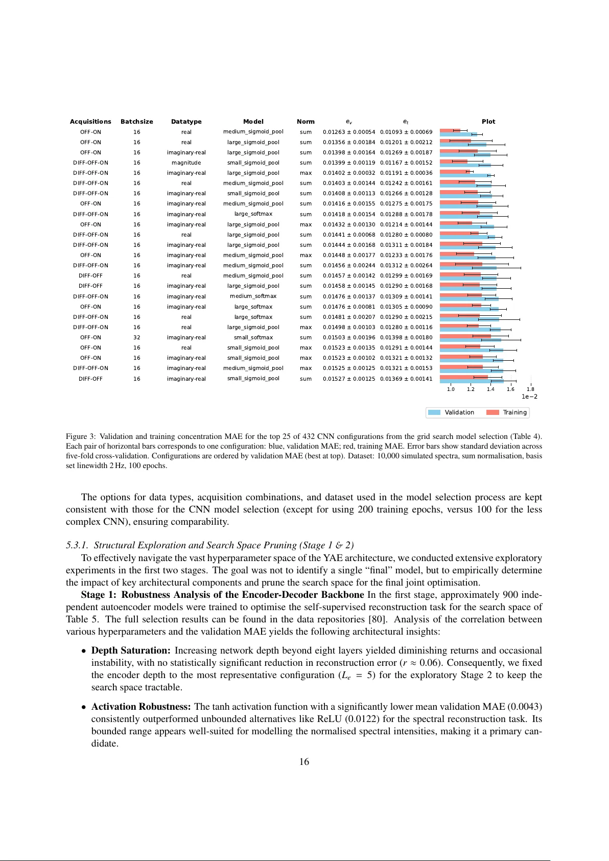
The Sim-to-Real Gap in MRS Quantiﬁcation: A Systematic Deep Learning V alidation for GAB A Zien Ma a , S. M. Shermer b , Oktay Karaku ¸ s a , Frank C. Langbein a, ∗ a School of Computer Science and Informatics, Car di ﬀ University , Car di ﬀ , CF24 4A G, United Kingdom b F aculty of Science and Engineering, Swansea Univer sity, Swansea, SA2 8PP , United Kingdom Abstract Magnetic resonance spectroscopy (MRS) is used to quantify metabolites in vivo and estimate biomarkers for con- ditions ranging from neurological disorders to cancers. Quantifying low-concentration metabolites such as GABA ( γ -aminobutyric acid) is challenging due to low signal-to-noise ratio (SNR) and spectral ov erlap. W e inv estigate and validate deep learning for quantifying complex, low-SNR, overlapping signals from MEGA-PRESS spectra, devise a con volutional neural network (CNN) and a Y -shaped autoencoder (Y AE), and select the best models via Bayesian optimisation on 10 , 000 simulated spectra from slice-proﬁle-aware MEGA-PRESS simulations. The selected models are trained on 100 , 000 simulated spectra. W e v alidate their performance on 144 spectra from 112 e xperimental phan- toms containing ﬁ ve metabolites of interest (GABA, Glu, Gln, NAA, Cr) with known ground truth concentrations across solution and gel series acquired at 3 T under varied bandwidths and implementations. These models are fur- ther assessed against the widely used LCModel quantiﬁcation tool. On simulations, both models achie ve near -perfect agreement (small MAEs; regression slopes ≈ 1 . 00, R 2 ≈ 1 . 00). On experimental phantom data, errors initially in- creased substantially . Howe ver , modelling variable line widths in the training data signiﬁcantly reduced this gap. The best augmented deep learning models achie ved a mean MAE for GAB A over all phantom spectra of 0 . 151 (Y AE) and 0 . 160 (FCNN) in max-normalised relati ve concentrations, outperforming the con ventional baseline LCModel (0 . 220). A sim-to-real gap remains, b ut physics-informed data augmentation substantially reduced it. Phantom ground truth is needed to judge whether a method will perform reliably on real data. K eywor ds: Magnetic Resonance Spectroscopy, GAB A, MEGA-PRESS, Deep Learning, Bayesian Model Selection, Domain Shift, Phantom V alidation 1. Introduction Magnetic resonance spectroscopy (MRS) is a non-in vasi ve technique for quantifying metabolite concentrations in vivo , providing insights into cellular metabolism that can support diagnosis and monitoring across neurological and oncological diseases [1, 2, 3, 4, 5]. A biomarker of particular clinical interest is γ -aminobutyric acid (GAB A), the primary inhibitory neurotransmitter in the brain, whose dysregulation is implicated in numerous psychiatric and neurological disorders [1, 6, 7, 8, 9, 10, 11]. Accurate quantiﬁcation of lo w-concentration metabolites such as GAB A is, howe ver , challenging: the weak GABA signal is partially obscured by stronger resonances from more ab undant compounds such as N-acetylaspartate (NAA) and creatine (Cr), leading to substantial spectral overlap. Edited MRS techniques such as MEGA-PRESS (Mescher-Garw ood point-resolved spectroscopy editing) are therefore commonly employed to isolate the GAB A signal [12, 13, 14]. While spectral editing improves speciﬁcity , the required subtrac- tion of edit-OFF and edit-ON (hereafter OFF and ON) acquisitions reduces the signal-to-noise ratio (SNR) and may introduce artefacts, creating additional challenges for reliable, unbiased quantiﬁcation. Deep learning (DL) has been applied to address these problems, potentially improving accuracy and reducing expert-dri ven parameter tuning [15]. In practice, howe ver , DL methods face a major obstacle: the “sim-to-real” ∗ Corresponding author . Email addr ess: LangbeinFC@cardiff.ac.uk (Frank C. Langbein) gap between simulated training data and experimental measurements. Training robust models requires large, la- belled datasets. In vivo data are costly to acquire at scale, subject to ethical and logistical constraints, and crucially lack ground-truth metabolite concentrations, precluding fully supervised training and rigorous ev aluation [3, 16, 17]. Phantom datasets pro vide known concentrations b ut are expensi ve and time-consuming to prepare, calibrate (e.g. pH, temperature, relaxation), and scan under multiple conditions; covering all concentration combinations, line widths, and sequence variants would be impractical [18, 19]. As a result, most DL models are trained and selected on large collections of simulated spectra [20, 21, 22]. Simulations typically assume idealised hardw are, controlled acquisition parameters, and simpliﬁed baselines. Ex- perimental spectra, instead, show variations and artefacts from scanner-speciﬁc implementations, B0 / B1 inhomo- geneities, imperfect water suppression, and subtraction-related baseline distortions [19, 23, 24]. Models optimised exclusi vely on simulated data can therefore overﬁt to unrealistic training distributions and exhibit substantial esti- mation bias when applied to experimental spectra. Recent studies have highlighted this concern, reporting strong performance on simulations but de graded accuracy and calibration under domain shift [22, 25]. In this work, we directly address this validation challenge through a systematic inv estigation of DL-based quan- tiﬁcation of GAB A and related metabolites from MEGA-PRESS spectra. While GAB A is our primary target, we simultaneously quantify N AA, Cr, glutamate (Glu), and glutamine (Gln), which are integral to brain metabolism and function [26]. Building on MRSNet [21], we pursue three main objectiv es. Firstly , we dev elop two complemen- tary architectures for multi-metabolite regression: a con volutional neural network (CNN) that captures local spectral features and a Y -shaped autoencoder (Y AE) that learns a denoised latent representation. Secondly , we perform system- atic model selection via Bayesian optimisation on a slice-proﬁle-aware simulated dataset (ﬁve-fold cross-validation on 10 , 000 spectra) to identify the best performing conﬁgurations of these models, and include several established ar- chitectures from the literature as comparati ve baselines (using their published conﬁgurations with minimal adaptation to our MEGA-PRESS pipeline). Thirdly , we assess the performance of the best DL models by v alidating them on 144 spectra from 112 experimental phantoms with known ground-truth concentrations (solutions and tissue-mimicking gels acquired at 3 T containing GAB A, Glu, Gln, Cr, NAA and no macromolecule background or lipid signal), and comparing their performance to the widely used LCModel tool (applied to OFF spectra as it provided the better quan- tiﬁcation results on the phantom data). For the baseline (ﬁxed-line width, non-augmented) models, across all 144 phantom spectra, mean MAE ov er all spectra for GAB A was 0 . 161 (MRSNet-Y AE), 0 . 203 (MRSNet-CNN), 0 . 167 (FCNN), and 0 . 220 (LCModel-OFF). Our results show that both architectures achiev e near-perfect agreement with ground truth on simulated data. On experimental phantoms, initial models showed a substantial sim-to-real gap. Howe ver , by incorporating realistic variability in spectral line widths into the training data, we signiﬁcantly improved rob ustness. The augmented models outperformed the con ventional LCModel baseline for GAB A and Glu; with linewidth augmentation, the best DL mod- els achiev ed GAB A MAE over all phantom spectra 0 . 151 (Y AE) and 0 . 160 (FCNN), outperforming LCModel-OFF (0 . 220), even if the sim-to-real gap could not be closed. Physics-informed simulation such as linewidth augmenta- tion is, hence, important for DL methods to generalise from simulation to experiment. W e argue that v alidation on phantoms with known concentrations should precede in vivo use of an y new quantiﬁcation method. Section 2 revie ws con ventional and machine learning-based quantiﬁcation methods in MRS. Section 3 details the simulated and experimental datasets and preprocessing. Section 4 describes our DL architectures, and Section 5 outlines the Bayesian optimisation-based model selection. Section 6 presents the experimental results; Section 7 concludes. 2. Related W ork The quantiﬁcation of metabolites from MRS spectra, particularly lo w-concentration compounds like GAB A, has motiv ated a wide range of analytical methods [16, 27, 28]. These fall into two main paradigms: (i) con ventional model- based ﬁtting with explicit basis functions and (ii) data-driv en machine learning, including deep learning (DL). W e focus on methods for edited spectra such as MEGA-PRESS and summarise their main de velopments and limitations, in particular interpretability , uncertainty quantiﬁcation, and behaviour under domain shift. 2 2.1. Conventional Quantiﬁcation Methods Con ventional quantiﬁcation in MRS is dominated by peak ﬁtting and spectral basis set methods. Peak ﬁtting mod- els spectral peaks using analytical lineshapes (e.g., Gaussian, Lorentzian, V oigt), adjusting parameters like amplitude and phase to match the data and estimating metabolite concentrations from peak areas. While some tools, such as L WFIT [18], use model-free integration over ﬁx ed frequency intervals for robustness, others, such as GANNET [29] and its successor Osprey [30], specialise in edited spectra like MEGA-PRESS by ﬁtting Gaussian models to target peaks. Although e ﬀ ectiv e for well-separated signals, peak ﬁtting accuracy is often compromised by spectral overlap and baseline distortions. Basis set ﬁtting methods model the acquired spectrum as a linear combination of basis spectra, which are pre- acquired from phantom experiments or generated from quantum-mechanical simulations. Using ﬁtting algorithms such as constrained nonlinear least-squares, these methods determine the relative contrib utions of each metabolite. A variety of such tools exist, operating either in the frequency (e.g., LCModel [31, 32], INSPECT OR [33], VESP A [34], JMR UI [35], A QSES [36], AMARES [37]) or time domain (e.g., QUEST [38], T ARQUIN [39, 40]), as revie wed in [41]. Recent toolboxes also o ﬀ er Bayesian posterior estimates over concentrations (e.g., FSL-MRS [42]), improving uncertainty characterisation relativ e to point estimates. Despite their widespread use, these methods face sev eral challenges. Simulated basis sets may not fully capture the nuances of experimental spectra [43], and performance can degrade with lo w signal-to-noise ratio or increased spectral line width [44, 45, 46]. Experimentally acquired basis sets can improv e accuracy , b ut their generation is laborious and requires signiﬁcant human e xpertise for preprocessing and parameter tuning, introducing operator-dependent variability [17]. Furthermore, challenges such as macromolecule contamination and ensuring consistency across di ﬀ erent modelling choices persist [47, 48]. 2.2. Machine Learning Methods Machine learning and particularly Deep learning (DL) hav e been proposed as an alternative that can automate analysis and reduce dependence on manual tuning and operator-dependent variability . Models trained on large-scale simulated datasets hav e been shown to learn rele vant features and predict metabolite concentrations directly from spectral data [21, 22, 25, 49, 50, 51, 52, 53, 54, 55]; other work uses DL for denoising before conv entional linear least-squares (LLS) or linear combination model (LCM) quantiﬁcation [49, 50, 54, 55, 56]. W e group existing DL- based quantiﬁcation strategies into three categories. A revie w of machine learning applications in MRS can be found in [57]. Direct Regression Appr oaches: The most direct application of DL frames quantiﬁcation as an end-to-end re- gression task, where a network, typically a CNN, learns to map raw spectral data directly to metabolite concentra- tions [22, 25, 53]. V ariations on this theme include using handcrafted wavelet scattering features to provide more robust inputs to a shallow regression network [58]. These models are computationally e ﬃ cient and can be designed to provide uncertainty estimates. Howe ver , because they do not explicitly model the physics of spectral formation, they can lack interpretability and are prone to ov erﬁtting, especially in low-SNR regimes. Their estimation bias is often unknown, as most ha ve not been v alidated against experimental data with ground-truth concentrations. Physics-Inf ormed and Hybrid Models: T o improve interpretability and robustness, other approaches integrate physical knowledge of spectral composition into the DL frame work. One strategy inv olves using a CNN to predict a clean, metabolite-only spectrum, which is then quantiﬁed using a ﬁxed, non-trainable solver such as multiv ariable linear regression against a predeﬁned basis set [54, 55, 59, 60]. A key limitation here is that errors from the quan- tiﬁcation step cannot be backpropagated to train the feature extractor . More advanced methods overcome this by incorporating a fully di ﬀ erentiable solver into the network architecture. For example, Q-Net [49] embeds a di ﬀ eren- tiable least-squares solv er , while PHIVE [61] inte grates a di ﬀ erentiable LCM into a v ariational autoencoder , enabling end-to-end training and robust uncertainty estimation. These models more tightly link representation learning with the quantiﬁcation task, but are more comple x to train and require access to accurate basis sets. Heuristic and Partially Di ﬀ erentiable Models: A third category of methods uses DL for feature extraction or parameter estimation but relies on ﬁxed or heuristic components for the ﬁnal quantiﬁcation. For instance, some models use a denoising autoencoder to learn a robust spectral representation but decode it using a ﬁxed LCM with a standard basis set [56]. Other encoder-decoder designs extend this approach. For example, Zhang et al. proposed a model using W av eNet blocks and an attention-based GR U to learn a robust latent representation from multi-echo JPRESS data, from which it simultaneously predicts concentrations, reconstructed FIDs, and phase parameters in an 3 end-to-end manner [62]. Others use a CNN to estimate spectral parameters (e.g., peak locations and widths) and then reconstruct the spectrum using a ﬁxed but di ﬀ erentiable physical model, such as a sum of Lorentzian functions [63]. A di ﬀ erent approach is taken by NMRQNet [64], which uses a recurrent network to predict spectral parameters and then reﬁnes them with a non-di ﬀ erentiable stochastic optimisation algorithm. While these methods can enforce physical plausibility , the separation between the learned and ﬁxed components prev ents global error minimization and limits end-to-end optimisation. Con ventional LCM methods remain interpretable and can provide uncertainty estimates but depend on accurate basis sets and can be sensitive to linewidth and baseline [45, 46]. Direct-regression DL is fast and ﬂexible but often lacks calibrated uncertainty and has rarely been validated on experimental ground truth [22, 52]. Physics-informed and di ﬀ erentiable hybrids improv e interpretability and gradient ﬂo w [49, 61] but still rely on basis accuracy and remain under-v alidated on phantoms. Recent revie ws of ML for proton MRS (e.g. V andesande et al. [57]) describe progress in denoising, quantiﬁcation, and uncertainty , and note remaining concerns about generalisation and bias under domain shift [52]. Many DL studies report strong performance on simulations or on in vivo data without ground truth; few provide v alidation on experimental phantoms with kno wn concentrations. 2.3. Limitations of Existing W ork and Our Contribution Con ventional and machine learning methods su ﬀ er from a lack of validation against known ground truth. Many DL-based studies rely exclusi vely on simulated data for ev aluation, using pre-set concentrations as ground truth [22, 25, 53, 58]. Others use in vivo data, which lacks ground truth, and instead compare results to established methods such as LCModel [49, 51, 54, 55]. As recent work has highlighted, models validated solely on synthetic data often ov erﬁt and exhibit signiﬁcant estimation bias when applied to real-world spectra [22, 25]. Thus, neither approach provides a true measure of a model’ s practical utility . Our w ork addresses this validation g ap. W e e valuate DL models for MEGA-PRESS quantiﬁcation systematically: Bayesian model selection on simulations, then validation on 144 phantom spectra with known concentrations. W e dev elop two distinct architectures, a CNN and a novel Y -shaped autoencoder (Y AE), and optimise them through Bayesian hyperparameter search on a large simulated dataset. The main focus is validation of the selected models on experimental phantom spectra and comparison with LCModel (Section 3). W e compare our models to ground truth and to the widely used LCModel to assess the capabilities and limitations of deep learning for MEGA-PRESS quantiﬁcation. W ithout validation on phantoms with known concentrations, one cannot judge whether a new method will perform reliably on real data. 3. Simulation, Phantom Experiments, and Evaluation Metrics Our study focuses on quantifying ﬁ ve metabolites (GAB A, Glu, Gln, N AA, and Cr) from edited spectra acquired with the MEGA-PRESS pulse sequence, which yields OFF and ON acquisitions and their di ﬀ erence (DIFF; the ON minus OFF di ﬀ erence spectrum). GAB A is the primary target; Glu and Gln are ke y e xcitatory neurotransmitters; N AA and Cr serve as prominent reference metabolites whose distinct peaks support calibration and relati ve quantiﬁcation. Concentrations are often reported relative to N AA or Cr . Below , we describe the simulated and e xperimental datasets, preprocessing, and ev aluation metrics. 3.1. Simulated Datasets T o train and validate the models, we generated simulated spectra by taking a weighted sum of simulated basis spectra for each metabolite. OFF and ON spectra for each metabolite were generated using custom MA TLAB code and the FID-A toolbox [20]. The simulations are based on Hamiltonian models for the molecules of interest and in volve solving the time-dependent Schrödinger equation for the MEGA-PRESS pulse sequence, calculating the pre- dicted time-domain echo signals, and adding line broadening to enhance realism. For some molecules, competing Hamiltonian models exist, including the Govindaraju, Kaiser , and Near models [65, 66, 67]. In this work, we used the Near model for GABA because the spectra it produces most closely match our experimental data, and there is a consensus that it is the preferred model [17]. Spatial localisation for MEGA-PRESS spectra is commonly achieved using a technique similar to PRESS (Point RESolved Spectroscopy). This process begins with an initial radiofrequency pulse that excites a slab-shaped region, 4 providing localisation in one dimension. This is followed by two subsequent refocusing pulses, each designed to se- lectiv ely refocus spins within a slab perpendicular to the pre viously e xcited slab and to each other . Consequently , only spins in the intersection of these three orthogonal slabs experience the complete sequence and contribute to the ﬁnal signal. Crusher gradients further enhance voxel localisation. Slice-selectiv e excitation is achie ved by applying ﬁnite- bandwidth modiﬁed sinc pulses concurrently with gradients. Many simulations neglect this, implementing excitation and refocusing pulses as ideal 90 ◦ and 180 ◦ rotations, respecti vely . Howe ver , this ignores the non-uniformity of exci- tation and refocusing pulse proﬁles, especially for large vox el sizes. T o obtain more realistic spectra, we performed simulations on a 2D spatial grid to more accurately model the excitation proﬁles of the refocusing pulses, thereby improving the realism of the simulated spectra. Finally , phase cycling w as implemented, cycling ov er two phases (0 ◦ , 90 ◦ ) each for the ﬁrst editing and the refocusing pulses, and four phases (0 , 90 , 180 , 270) for the second editing pulse, resulting in 2 × 2 × 2 × 4 = 32 simulation runs for each point on the spatial grid, and a total of 32 × 8 × 8 = 512 simulations for each metabolite spectrum. T o simulate both the ON and OFF spectra for each metabolite therefore requires 1 , 024 simulation runs. See Figure 1 and mrsnet/simulators/fida/run_custom_simMegaPRESS_2D.m in [68] for details. The simulation produces a complex time-domain signal corresponding to the time-e volution of the x and y compo- nents of the transv erse magnetisation, which is Fourier-transformed to obtain a spectrum. In practice, the time-domain signal is multiplied by an exponential en velope to simulate signal attenuation due to T 1 and especially T 2 relaxation e ﬀ ects. The decay rate of the exponential function controls the linewidth of the simulated spectra. Lorentzian ﬁts of the N AA peak in 144 experimental MEGA-PRESS OFF spectra yielded a median linewidth of just under 2 Hz and a mean just over 2 Hz (full width at half maximum, FWHM). Based on this, we chose a line width of 2 Hz FWHM for the simulated basis spectra as a realistic but slightly conservati ve value. Estimated linewidths across the 144 phantom spectra span approximately 1 Hz to 10 Hz FWHM (see the sim-to-real repository [69]); we use this range when assessing variable line width augmentation in Section 6.2. Consistently , our sim-to-real analysis on the phantom series [69] indicates that simulations with a ﬁxed 2 Hz FWHM basis pro vide the closest o verall match in spectral mag- nitude and linewidth to the phantom data, and allowing the simulated line width to vary did not materially reduce the sim-to-real gap in these spectral similarity metrics. In Section 6.2, we show that linewidth augmentation can improv e quantiﬁcation performance. 3.2. Concentration Sampling and Noise Injection W e adopt the same strategy for generating synthetic spectra as in our previous work [21], where training and validation samples are constructed by taking linear combinations of individual metabolite signals from a giv en basis set. Each metabolite is assigned a scaling factor within the range [0 , 1], representing its relativ e concentration. These concentration v alues are sampled using a Sobol sequence: a lo w-discrepancy , quasi-Monte Carlo method that ensures uniform co verage of the high-dimensional concentration space e ven with a relati vely small number of samples. Sobol sampling gi ves more uniform cov erage of the concentration space than random sampling, which helps the models cope with div erse spectral mixtures. T ime-domain Gaussian noise with zero mean and standard de viation σ sampled uniformly in [0 , 0 . 03] is added to all simulated spectra, whose signal amplitudes are normalised so the maximum spectral peak equals 1 . 0. This noise lev el reﬂects realistic scanner-induced variability and was pre viously sho wn to closely approximate noise observed in experimental phantom spectra [18, 21]. The range was guided by expert analysis of spectral regions that contain no identiﬁable metabolic signal, capturing acquisition-related baseline ﬂuctuations. Beyond mimicking experimental conditions, randomised noise both improv es realism and reduces ov erﬁtting to noise-free inputs. W e veriﬁed the interval on our 144 phantom spectra by estimating σ from signal-free regions only in the phantom–simulation residual: median σ ≈ 0 . 014, ≈ 80% within [0 , 0 . 03]. The 30 spectra with σ > 0 . 03 come from the gel series E4, E9, and E11 (di ﬀ erent bandwidths or reacquired later) and the solution series E6; E6 and E11 are the noisiest. These series were included to test performance across SNR. For the main training runs reported in this paper , the simulated data use the above setup: slice-proﬁle-aware basis spectra with ﬁxed 2 Hz linewidth, Sobol-sampled concentrations, time-domain Gaussian noise in [0 , 0 . 03], and the same B0 alignment, ppm range, and amplitude normalisation as in the common export pipeline (Section 3.4). W e did not apply explicit augmentation for frequency drift, higher -order phase errors, v ariable line width beyond the ﬁx ed simulation v alue, synthetic rolling baselines, or non-Gaussian noise. The impact of more aggressive augmentation, speciﬁcally using varied line widths, is explored in Section 6.2 and further discussed in Section 7. 5 (a) Sequence Diagram for MEGA-PRESS (b) Simulation Grid (2D) for cubic voxel with a = 3 cm Figure 1: The sequence diagram (a) shows the RF and gradient pulses with actual pulse shapes and timings used in the simulations. The initial excitation pulse is modelled as an ideal (instantaneous) slice-selective 90 ◦ pulse and the corresponding slice selection gradient G z is therefore omitted. The excitation pulse excites a slice of thickness 3 cm perpendicular to the z -axis. The refocusing pulses refocus the magnetisation of 3 cm thick slabs perpendicular to the x and y axis, respectively , to deﬁne the localised vox el. What di ﬀ erentiates the MEGA-PRESS sequence from the standard PRESS sequence is the presence of two 20 ms frequency-selectiv e Gaussian editing pulses (yellow and green) at 1 . 9 ppm for the ON acquisition. For the OFF spectra the editing pulses could in principle be omitted, but the simulation follows the experimental implementation where editing pulses at 7 . 5 ppm, which have no e ﬀ ect on the metabolites of interest, are applied instead. The readout of the signal starts at 68 ms as indicated. Experimentally , it can last over 1 s, depending on the dwell time and number of samples acquired. For a bandwidth of 2000 Hz, the dwell time is 0 . 5 ms and acquiring N = 2048 samples, a typical signal length, would therefore require 2048 × 0 . 5 ms = 1 . 024 s. The readout block in the diagram is truncated at 80 ms for clarity , to show the RF pulses and timings. T o account for imperfect slice proﬁles of the refocusing pulses, the spectra are simulated on a spatial grid (b) and the av erage over all positions is calculated. 3.3. Experimental Dataset In addition to v alidation on simulated spectra, we e valuate our models’ performance on experimental spectra from test objects with known metabolite concentrations, ranging from bu ﬀ ered metabolite solutions to tissue-mimicking gel phantoms. These phantoms contain only the speciﬁed metabolites, and no macromolecule (MM) or lipid signal, unlike in vivo spectra. Sev eral sets of experiments were conducted, ranging from bu ﬀ er solutions with a few metabolites to tissue- mimicking gel phantoms with sev eral relev ant metabolites. All phantoms were prepared in-house at the Institute for Life Science at Swansea University . For the solution datasets, the general procedure was to prepare a pH-neutral phosphate bu ﬀ er solution and add ﬁxed amounts of various metabolites to obtain a base solution. Some of the base solution was then used to prepare “spiked” solutions with high concentrations of a single metabolite, typically GAB A, our primary interest. The solution series were then generated by incrementally removing a small amount of solution from the phantom and replacing it with the same volume of a spiked solution. This procedure allows for increasing the concentration of a single metabolite in small increments without changing the baseline concentration of others, providing more precise control ov er concentrations than if the solutions were prepared independently . After each addition of spiked solution, a ne w OFF and ON spectrum was acquired. The gel phantoms were obtained similarly by preparing base solutions and adding small amounts of spiked metabolite solutions to v ary concentrations. Howe ver , separate gel phantoms were prepared for each combination of concentrations, as incremental addition is not feasible for gels. T o create gels, a gelling agent (Agar Agar, 1 g per 100 ml) was added to each solution, and the mixture was heated to approximately 95 ◦ C. The hot solutions were then transferred to suitable molds and allowed to cool to room temperature and solidify before scanning. The composition of the phantoms was intentionally varied in complexity . In total, 144 spectra were obtained from 112 phantoms (some phantoms were scanned multiple times—e.g. E4 and E9—yielding more spectra than physical objects). Solution series E1 had the simplest composition, with only ﬁxed concentrations of N AA and Cr and 6 increasing amounts of GABA, and no Glu or Gln. Solution series E2 was similar but deliberately miscalibrated with a lo w pH to test the models’ ability to cope with miscalibrated data. Solution series E3 w as similar to E1 b ut included ﬁxed amounts of Glu and Gln. Series E4 consisted of gel phantoms with ﬁxed amounts of N AA, Cr , Glu, and Gln, and varying amounts of GABA, with concentrations similar to E3. The gel phantoms were scanned four times. The ﬁrst two rounds (E4a and E4b) were acquired on the same day with the same sequence but two di ﬀ erent acquisition bandwidths. The phantoms were scanned again with the same sequence and bandwidths a week later to acquire more data and assess any deterioration over time (E4c, E4d). E6 and E7 were solution series similar in composition to E3, while E8, E9, E11, and E14 were gel phantoms similar to E4. Not all av ailable experimental series were included, as some in volv ed additional metabolites for other projects. A summary of the metabolite concentrations for the experimental series is in T able 1, and further details on phantom design can be found in [18]. All spectra were acquired on a Siemens MA GNETOM Skyra 3T MRI system at Swansea Univ ersity’ s Clinical Imaging Unit. Datasets E1 to E4 used the Siemens WIP MEGA-PRESS implementation for GAB A editing, while the remaining datasets (E6, E7, E8, E9, E11, and E14) were acquired with a widely used implementation from the University of Minnesota [70]. As GAB A is our main metabolite of interest, most experimental series kept the concentrations of N AA, Cr , Gln, and Glu constant while gradually increasing GABA concentration, except for E9, where all metabolite concentrations were varied. All spectra were acquired with T E = 68 ms and T R = 2000 ms with 160 av erages and N = 2048 time samples per spectrum. The sampling frequency w as 1250 Hz for experiments E1, E2, E3, E4a, and E4c, and 2000 Hz for E4b, E4d, E6, E7, E8, E9a, E9b, E11, and E14. These parameters were chosen as they are generally optimal for GAB A editing. The sampling frequencies are determined by the dwell time of each measurement. Shorter dwell times allow for faster data acquisition and a broader spectral frequency range, but also reduce the signal-to-noise ratio (SNR). 2000 Hz (dwell time 0 . 5 ms) is the most common sampling frequency at 3 T, but 1250 Hz (dwell time 0 . 8 ms) still cov ers the frequency range of interest with slightly better SNR, which is why both values were used. For ev ery MEGA-PRESS run, the acquired time series data was Fourier -transformed, frequency and phase- corrected, and av eraged to create three spectra: OFF , ON, and DIFF. This was done using a combination of vendor- supplied scanner software and in-house MA TLAB code. Acquisition parameters and reconstruction details are de- scribed in [18]. 3.4. Prepr ocessing the Datasets All experimental (phantom) and simulated spectra are processed with a harmonised pipeline so that inputs pre- sented to the models share an identical ppm axis, spectral resolution and scaling. Only the data-origin steps di ﬀ er; the subsequent export to model inputs is identical across datasets. For experimental spectra only , the complex free-induction decays (FIDs) for the OFF and ON acquisitions are read. Processing proceeds in the time and then frequency domain: 1. Apodization: no windowing is applied, as it did not improv e downstream performance in our data (Ham- ming / Hanning windowing w as tried). 2. Phase handling: when real / imaginary channels are used, we explored applying a linear phase correction (con- stant and linear terms in frequency) estimated by minimising the imaginary component or spectral entropy of the real part. As no signiﬁcant improv ement was observed, we did not use this for training the models. 3. W ater-peak attenuation: around the water resonance (4 . 75 ppm ± 0 . 75 ppm window), lar ge outliers are clamped tow ards the local median in the magnitude spectrum to reduce residual water without altering phase. 4. B0 alignment across acquisitions: a single frequency shift (ppm) is estimated per spectrum from a reference metabolite. W e examine NAA (2 . 01 ppm) and Cr (3 . 015 ppm) within narrow windows ( ± 0 . 25 ppm) and use Jain’ s method [71] to estimate the exact peak location in the Fourier spectrum. The reference peak with higher prominence is used, and the resulting shift is applied uniformly to OFF , ON and DIFF. Residual misalignment after resampling is negligible at the chosen resolution. 5. Di ﬀ erence spectrum: DIFF is computed as ON − OFF after the abov e steps to ensure consistency with aligned acquisitions. Simulated spectra required less pre-processing. For consistency with the experimental spectra, we apply B0 alignment in the same way as for the experimental spectra after noise has been added and DIFF is recomputed. No water suppression or additional phase correction is applied. 7 T able 1: Composition of the experimental data: 144 spectra from 112 phantoms (phantom count is the sum of the ﬁrst number in each row , ignoring the repetition factor when given as e.g. 1 × 2 or 8 × 4). For E4, 8 × 4 denotes 8 gel phantoms each scanned in four acquisition rounds (E4a–E4d). Concentrations are in mM = mmol / L. E1 contains a phantom with NAA only and a phantom with NAA and Cr only , followed by phantoms with increasing amounts of GABA (Cr indicated by 0 / 8 . 0 where applicable). E4 phantoms were acquired four times with di ﬀ erent bandwidths (E4a / c: 1250 Hz, E4b / d: 2000 Hz) and reacquired one week later (E4c / d). E9 consists of 7 phantoms with varying concentrations of all metabolites; one phantom was scanned three times (1 × 3) and the rest twice (1 × 2), so that E9a contains one more spectrum than E9b. Series Medium # Phantoms N AA Cr Glu Gln GAB A E1 Solution 13 15 . 0 0 / 8 . 0 0 . 0 0 . 0 0 . 00, 0 . 52, 1 . 04, 1 . 56, 2 . 07, 2 . 59, 3 . 10, 4 . 12, 6 . 15, 8 . 15, 10 . 12, 11 . 68 E2 Solution 1 15 . 0 0 . 0 0 . 0 0 . 0 0 . 0 15 15 . 0 8 . 0 0 . 0 0 . 0 0 . 00, 0 . 50, 1 . 00, 1 . 50, 2 . 00, 2 . 50, 3 . 00, 3 . 99, 4 . 98, 5 . 96, 6 . 95, 7 . 93, 8 . 90, 9 . 88, 11 . 81 E3 Solution 15 15 . 0 8 . 0 12 . 0 3 . 0 0 . 00, 1 . 00, 2 . 00, 3 . 00, 3 . 99, 4 . 98, 5 . 97, 6 . 95, 7 . 93, 8 . 91, 9 . 88, 10 . 85, 11 . 81, 12 . 77, 13 . 73 E4 Gel 8 × 4 15 . 0 8 . 0 12 . 0 3 . 0 0 . 00, 1 . 00, 2 . 00, 3 . 00, 4 . 00, 6 . 00, 8 . 00, 10 . 00 E6 Solution 10 15 . 0 8 . 0 12 . 0 3 . 0 0 . 00, 1 . 03, 2 . 05, 3 . 06, 4 . 07, 6 . 09, 8 . 09, 10 . 08, 12 . 05, 14 . 98 E7 Solution 16 12 . 0 7 . 0 12 . 0 3 . 0 0 . 00, 1, 2, 2 . 99, 3 . 98, 4 . 97, 5 . 95, 6 . 93, 7 . 9, 8 . 87, 9 . 84, 10 . 80, 11 . 76, 12 . 71, 13 . 66, 14 . 61 E8 Gel 8 15 . 0 8 . 0 12 . 0 3 . 0 0 . 00, 1 . 00, 2 . 00, 3 . 00, 4 . 00, 6 . 00, 8 . 00, 10 . 00 E9 Gel 1 × 2 14 . 0 8 . 0 2 . 0 11 . 0 6 . 0 1 × 2 8 . 0 7 . 0 7 . 0 13 . 0 4 . 0 1 × 2 10 . 0 6 . 0 6 . 0 8 . 0 6 . 0 1 × 2 12 . 0 9 . 0 2 . 0 14 . 0 4 . 0 1 × 3 11 . 0 8 . 0 3 . 0 10 . 0 3 . 0 1 × 2 15 . 0 10 . 0 4 . 0 9 . 0 5 . 0 1 × 2 13 . 0 7 . 0 5 . 0 12 . 0 2 . 0 E11 Gel 8 12 . 0 7 . 0 12 . 0 3 . 0 0 . 00, 1 . 00, 2 . 00, 3 . 00, 4 . 00, 6 . 00, 8 . 00, 10 . 00 E14 Gel 11 11 . 8 6 . 3 8 . 55 2 . 25 0 . 00, 1 . 02, 2 . 05, 3 . 06, 4 . 08, 5 . 09, 6 . 1, 7 . 1, 8 . 1, 9 . 1, 10 . 09 Independent of their origin, spectra are prepared for training and inference using the same steps: 1. Fixed ppm band and resolution: signals are zero-ﬁlled / truncated in time and FFT -transformed; the frequency- domain spectra are then oriented to a common descending ppm axis and cropped to [4 . 5 ppm , 1 . 0 ppm] with exactly 2048 points. This harmonises datasets acquired at di ﬀ erent bandwidths (e.g., 1250 Hz vs 2000 Hz) without altering linewidths; zero-ﬁlling does not change SNR but provides a common sampling grid. The ppm axis direction is consistent across all inputs. 2. Amplitude normalisation: each spectrum is scaled by the maximum magnitude of its OFF acquisition when av ailable; otherwise by the global maximum across provided acquisitions. This yields a comparable dynamic range across samples and acquisitions. 3. Inputs and channels: for each acquisition (OFF , ON, DIFF) we can export real, imaginary and / or magnitude channels, providing up to nine channels; the channel combination and acquisition selection used by the best CNN and Y AE conﬁgurations are reported in Section 5. 4. Baseline handling: beyond the water-windo w attenuation, no explicit baseline modelling or subtraction is ap- plied. In particular , the DIFF baseline is retained so that the models learn to accommodate realistic baselines present in both simulated and experimental data. 5. T argets (for supervised training): ground-truth values are exported as an ordered vector ov er the metabolites. Concentrations are expressed relati ve to N AA as reference, so the N AA entry equals 1 by construction. During model selection, we considered sum-normalisation (v ector divided by its sum) and max-normalisation (di vided by its maximum), a common normalisation step to account for v ariations in total signal or reference metabolite concentrations [72]. The normalisation and channel choices for the selected best models are giv en in Section 5; 8 ev aluation metrics in Section 3.5 use max-normalised concentrations. These steps ensure that spectra presented to the models are aligned in ppm, uniformly sampled, consistently scaled and represented in a common acquisition-channel format across experimental and simulated datasets. 3.5. P erformance Evaluation Performance is ev aluated in terms of spectral reconstruction (denoising) and metabolite quantiﬁcation accuracy . For architectures that output a reconstructed spectrum (our Y AE), denoising is assessed by the mean absolute error between the noise-fr ee (clean) spectrum and the model’ s reconstruction from the noisy input: ϵ spec = 1 F F X f = 1 | x f − ˆ x f | (1) where x f is the clean reference value at frequency bin f , ˆ x f is the reconstructed value, and F is the number of frequency points. This quantiﬁes how well the model suppresses noise while preserving spectral structure. Quantiﬁcation performance is ev aluated using the mean absolute error (MAE) o ver maximum-normalised concen- trations, ϵ = 1 N N X l = 1 | g l − p l | (2) where g l is the ground-truth and p l the predicted concentration of metabolite l , and N is the number of metabolites. W e use maximum-normalised concentrations for e valuation regardless of the normalisation used during training, as MAE in this space is rob ust to outliers and comparable across datasets. Where appropriate, we also report error distributions, mean and standard de viation. T o assess systematic bias and scale, we ﬁt a linear regression of predicted vs. ground-truth concentrations, y = a x + q . Ideal performance corresponds to slope a = 1 and intercept q = 0. W e report the slope, intercept, coe ﬃ cient of determination R 2 , standard error of the ﬁt, and p -v alue for the regression. T ogether , MAE and regression metrics characterise both the magnitude of errors and any consistent o ver- or under -estimation. 3.6. Experimental Gr ound-T ruth V alidation The ground truth for the experimental spectra is the millimolar concentrations of the metabolites. Because the algorithms output only normalised concentrations and conv ersion to millimolar would require additional calibration, we evaluate relativ e concentrations (ratios eliminate arbitrary scaling). NAA is chosen as a reference for the relati ve concentrations as it has a prominent peak in both the OFF and DIFF spectra and relati vely stable peak characteristics. Alternativ ely , Cr could be used as a reference, b ut N AA is preferable here because the Cr signal is absent in the DIFF spectra. Once the relati ve concentrations hav e been calculated, the mean absolute error (MAE) is used to measure the prediction error for each metabolite; when reported ov er the phantom set, we use the mean absolute error ov er all spectra (ov erall MAE) or, for experiment-lev el comparison, the mean over spectra within each series (Section 3.7). The standard de viation (SD) is used to reﬂect the variability of the prediction error . Linear regression ﬁtting and statistical analysis are performed for the relativ e concentrations in the same manner as detailed above. Finally , we compare our quantiﬁcation results with LCModel, one of the most widely used tools for in vivo MRS quantiﬁcation. LCModel was run separately on the OFF and DIFF spectra of each phantom. F or a fair comparison with the DL models, LCModel was conﬁgured with a basis set derived from the same FID-A simulations and Hamil- tonian choices used to generate the DL training data (Section 3.1), including the Near model for GAB A. Fitting range, baseline model (spline), and other settings were chosen to match typical MEGA-PRESS practice; further details (v er- sion, ﬁtting range, baseline parameters) are given in the benchmark study [18]. T able 10 compares quantiﬁcation accuracy of LCModel-OFF and LCModel-DIFF across e xperiments; LCModel-OFF achie ved lo wer experiment-le vel errors for GAB A and Glu, and is therefore used as the main con ventional baseline in the following comparisons. W e use LCModel-OFF as the conv entional baseline because it gav e lower errors than LCModel-DIFF on our phantom data (T able 10), so the DL models are compared against a strong rather than a weak baseline; this aligns with lit- erature suggesting o ﬀ -resonance spectra can yield more reliable quantiﬁcation than di ﬀ erence spectra under certain conditions [73]. 9 3.7. Statistical Comparison of Quantiﬁcation Err ors T o compare the quantiﬁcation accuracy between models on phantom data in a statistically principled and model- agnostic manner, we further analyse the distributions of absolute quantiﬁcation errors across experiments, where a single experiment here refers to one series in the phantom data. Since absolute errors are non-negati ve and typically non-Gaussian, all statistical analyses are based on non-parametric methods. T o avoid pseudo-replication arising from treating spectra acquired under identical experimental conditions as independent samples, each experiment is treated as the fundamental statistical unit. Thus, experiment-lev el MAE denotes the mean error over spectra within each series (one v alue per series per metabolite), whereas ov erall MAE denotes the mean error ov er all 144 spectra as used later in summary T ables 12 and 13. For a giv en experiment e and metabolite m , the mean absolute error across spectra is computed as ˜ ϵ e , m = 1 K e K e X k = 1 ϵ e , k , m , (3) where K e denotes the number of spectra in experiment e . The mean provides a standard summary of typical error magnitude per experiment. Paired one-tailed W ilcoxon signed-rank tests are then applied to the experiment-le vel aggregated errors to assess whether one model consistently yields lower quantiﬁcation errors than another across experiments. This paired for- mulation exploits the fact that both models are e valuated under identical experimental conditions, thereby isolating di ﬀ erences attributable to the quantiﬁcation method. In addition to hypothesis testing, e ﬀ ect sizes are reported to facilitate direct interpretation of performance di ﬀ er- ences. Speciﬁcally , the proportion of experiments with lo wer error, P e = 1 E E X e = 1 I  ˜ ϵ (1) e , m < ˜ ϵ (2) e , m  , (4) quantiﬁes the fraction of e xperiments in which one model outperforms the other, while the mean di ﬀ erence in absolute error , ∆ m = 1 E E X e = 1  ˜ ϵ (1) e , m − ˜ ϵ (2) e , m  , (5) indicates the direction and magnitude of the performance di ﬀ erence. W e use these metrics to compare models con- sistently: MAE and regression slope / intercept for magnitude and bias, and e xperiment-level W ilcoxon tests and e ﬀ ect sizes for statistical comparison. 4. Deep Learning Architectur es This section describes the deep learning architectures ev aluated here. W e ﬁrst present our two proposed architectures— a con volutional multi-class regressor (CNN) and a Y -shaped autoencoder (Y AE)—which are extensiv ely parame- terised and optimised via Bayesian model selection (Section 5). W e then describe sev eral comparative baselines from the literature, implemented with their published conﬁgurations and minimal adaptations to our MEGA-PRESS pipeline. The CNN builds on the architecture of [21] and consists of 1D and 2D con volutions that extract features along the frequency axis and across acquisition channels, followed by fully connected layers that regress to metabolite concentrations. W e explore a broader architectural space (kernel sizes, down-sampling, regularisation, acti vations) to identify an optimal conﬁguration. The Y AE is a two-branch network: an encoder maps the input to a latent representation; one branch (decoder) reconstructs a denoised spectrum, and the other (quantiﬁer) re gresses the latent representation to concentrations. This design is motiv ated by the physical principle that an MRS spectrum is a linear combination of basis spectra: the autoencoder encourages a latent space that captures the weights of these basis components, which the quantiﬁer then maps to concentrations. The decoder acts as a regulariser , ensuring the latent representation retains su ﬃ cient spectral information for reconstruction. 10 T able 2: Parameterised con volutional multi-class regressor (CNN) architecture with parameters. N f is the number of frequencies in the inputs, and channels refers to the number of input spectra. The parameters f 1 and f 2 determine the number of con volutional ﬁlters, k 1 , k 2 , k 3 and k 4 determine the kernel size of the conv olutions, s 1 and s 2 determine the use of strides or max-pooling, d 1 determines the use of dropout or batch normalisation, d 2 the dropout rate in the dense layer, and e the number of neurons in the dense layer . The activ ation function at the output is either sigmoid or softmax, and the output consists of N m metabolite concentrations (ﬁxed to 5). Layer Description input (channels, N f ) con v1 FCONV ( f 1 , (1 , k 1 ), s 1 , d 1 ) con v2 FCONV ( f 1 , (1 , k 2 ), s 1 , d 1 ) reduce Repeat until one output channel: FCONV( f 1 , (min(channels , 3), k 3 ), 1, d 1 ) con v3 FCONV ( f 1 , (1 , k 4 ), 1, d 1 ) con v4 FCONV ( f 1 , (1 , k 4 ), s 2 , d 1 ) con v5 FCONV ( f 2 , (1 , k 4 ), 1, d 1 ) con v6 FCONV ( f 2 , (1 , k 4 ), s 2 , d 1 ) dense1 sigmoid (Dense ( e )) dropout if d 2 > 0 . 0 then Dropout ( d 2 ) dense2 Dense (metabolites) activ ation sigmoid () or softmax () output N m FCONV ( f , k , s , d ) is a sequence of layers forming mainly a con volution, determined by its parameters as follo ws: if s ≤ 0 : x = Conv2D (filter= f , kernel_shape= k )( x ) else: x = Conv2D (filter= f , kernel_shape= k , strides = (1, s )) ( x ) if d == 0 . 0 : x = BatchNormalisation () ( x ) x = ReLU () ( x ) if d > 0 . 0 : x = Dropout ( d ) ( x ) if s < 0 : x = MaxPool2D ( (1 , | s | ) ) ( x ) For these architectures, the input can be chosen from ON, OFF , and DIFF acquisitions and from real, imaginary , or magnitude representations; see Section 3.4. The following subsections detail the CNN (Section 4.1), the Y AE (Section 4.2), and the additional baselines (Section 4.3). 4.1. CNN: Convolutional Multi-Class Re gressor Our parameterised CNN architecture is shown in T able 2. It consists of a sequence of conv olutional layers follo wed by two dense layers. Its input has a channel axis, for the di ﬀ erent acquisitions and datatypes, follo wed by a frequency axis for the bins from the Fourier transform; see Section 3.4. The con volutional blocks are represented by FCONV ( f , k , s , d ), a sequence of layers detailed in T able 2. This block primarily consists of a con volution with f ﬁlters, kernel size k , and a ReLU acti vation function. The parameter s controls dimensionality reduction along the frequency axis, using either strides (if s > 0) or max-pooling (if s < 0). The parameter d controls regularisation: dropout is used if d > 0, and batch normalisation is used if d = 0. This parameterisation enables us to explore di ﬀ erent strategies for down-sampling and regularisation during model selection. While batch normalisation addresses internal covariate shift to improve training, dropout regularisation addresses ov erﬁtting by learning more robust features. In practice, using both simultaneously is often redundant. The ﬁrst two layers are 1D conv olutions along the frequency axis (kernel sizes k 1 , k 2 ), applied per channel to detect local spectral features. A reduction module then collapses the channel dimension to one via sequential 2D con volutions with kernel size (min(channels , 3) , k 3 ), combining information across acquisitions; this channel-then- reduce design follows [21]. A further sequence of 1D conv olutions along the frequency axis on this single combined channel extracts higher -level spectral features. T wo dense layers (with sigmoid acti vation between them and optional dropout) map these features to concentrations via a ﬁnal softmax or sigmoid output. While softmax may match the relativ e concentrations better , sigmoid may be more suitable as the relativ e concentrations do not represent probabili- ties. The network is trained by minimising the mean squared error (MSE). T raining and model selection are detailed in Section 5. 4.2. Fully Connected Y -Shaped Autoencoder (Y AE) The Y AE is a deterministic, fully connected network with three modules: an encoder, a decoder, and a quantiﬁer (Figure 2, T able 3). W e use fully connected (rather than con volutional) layers to capture global spectral structure: in the frequency domain, information lies in ov erall lineshapes rather than local patterns, and CNNs’ locality bias can be misaligned with this. W e do not use a variational autoencoder (V AE) design because stochastic latents and V AE 11 Figure 2: Illustration of the Y -shaped autoencoder (Y AE) architecture. The input consists of one or more noisy MEGA-PRESS spectra (OFF , ON, DIFF using real, imaginary or magnitude representations). The encoder maps the input to a compressed latent representation. The decoder branch reconstructs denoised versions of the input spectra from this latent space. The quantiﬁer branch predicts the metabolite concentrations from the same latent representation. K ey components are highlighted: ① hidden layer activation function, ② dropout layer, ③ decoder output acti vation function, and ④ quantiﬁer output activ ation function. T able 3: Parameterised architecture for the Y AE’ s encoder, decoder , and quantiﬁer modules. The speciﬁc values explored for the parameters are giv en in Section 5. Channels refer to the number of channels used as input spectra. N f : number of frequency samples in the input spectrum. N q : number of neurons in the ﬁrst dense layer of the quantiﬁer . N m : number of output metabolite concentrations (ﬁxed to 5). L e , L d , L q : number of dense layers in the encoder, decoder, and quantiﬁer , respecti vely . a e , a d : activation function for the encoder and decoder . a q , a m : activation function for the hidden layers and output layer of the quantiﬁer . d e : dropout rate for the encoder . Encoder Layer Description input (channels , N f ) dense_e for each channel c: for l = 1 , . . . , L e − 1: Dense  N f 2 l − 1 , a e  Dropout ( d e ) latent_c Dense  N f 2 L e − 1 , a e  output  N f 2 L e − 1  per channel Decoder Layer Description input  N f 2 L e − 1  per channel dense_d for each channel c: for l = L d , . . . , 2: Dense  N f 2 l − 1 , a d  decode_c Dense  N f , a d  output ( N f ) per channel Quantiﬁer Layer Description input  N f 2 L e − 1  per channel ﬂatten channels × frequencies dense_q for l = 1 , 2 , . . . , L q − 1: Dense  N q 2 l − 1 , a q  quant Dense ( N m , a m ) output N m regularisation can reduce reconstruction ﬁdelity , which we need for precise quantiﬁcation. Input and output options match the CNN (Section 3.4): the decoder outputs a denoised spectrum; the quantiﬁer outputs normalised relativ e concentrations. For each channel of the input, the encoder consists of a sequence of fully connected layers, reducing the input frequency dimensions while enriching the feature representation in the latent space. As detailed in T able 3, each layer comprises N f 2 l − 1 neurons at the l -th layer , where N f denotes the initial frequency dimension. Dropout layers ( d e ) are applied after each dense layer for regularisation, so the model can be adapted to di ﬀ erent complexities and dataset sizes. The ﬁnal encoder layer compresses the input into a lo w-dimensional latent representation of size N f 2 L e − 1 per channel. The latent representation feeds into two separate branches, forming the “Y” shape. The ﬁrst branch is the decoder , which aims to reconstruct a denoised spectrum from the latent representation, restoring the original input shape of (channels , N f ). Its architecture consists of a sequence of fully connected layers that progressiv ely expand the data, structured to reverse the encoder’ s compression (T able 3). The decoder is used to ensure the latent representation contains su ﬃ cient features to reconstruct a clean spectrum, rather than for denois- ing. This is moti vated by the physical principle that an MRS spectrum is a linear combination of basis spectra (see Section 3.1) and the demonstrated e ﬃ cacy of denoising autoencoders in MRS [74, 75]. Dropout was not applied in the decoder module, as its objectiv e is to reconstruct the spectrum in a stable and deterministic manner; stochastic 12 regularisation here could disrupt reconstruction ﬁdelity . The second branch is the quantiﬁer , which regresses the latent representation to metabolite concentrations. The latent representation is ﬂattened across channels and frequency dimensions, then passed through a sequence of fully connected layers ( N q 2 l − 1 neurons at layer l ). W e do not use dropout in the quantiﬁer: the encoder already regularises the latent space, and dropout at the ﬁnal regression stage would add unnecessary stochasticity where a stable, deterministic mapping to concentrations is required. The decoder acts as a regulariser , as the encoder must retain enough spectral information such that the decoder can reconstruct the full spectrum. So the latent representation cannot collapse to quantiﬁcation-only features. As an MRS spectrum is a linear combination of basis spectra (Section 3.1), this aims to ensure the latent space reﬂects those weights. The ﬁnal output layer of the quantiﬁer maps the transformed features to N m target dimensions: the number of quantiﬁed metabolites. The Y -shape ties the latent representation to both reconstruction and quantiﬁcation, so the encoder is encouraged to learn features that support both tasks rather than ov erﬁtting to concentration targets alone. W e use the Huber loss for the decoder and quantiﬁer branches: S δ ( x , x ′ ) =        1 2 ( x − x ′ ) 2 , if | x − x ′ | ≤ δ , δ ( | x − x ′ | − 1 2 δ ) , otherwise. (6) where x is the ground truth, x ′ is the prediction, and δ is a hyperparameter . W e use δ = 1 . 0, the default value in T ensorFlow . When the absolute error is less than or equal to δ , the Huber loss is quadratic like MSE; for lar ger errors, it becomes linear like MAE. This makes the loss less sensitiv e to large errors and outliers compared to MSE. This choice is motiv ated by the nature of MRS data. For the decoder branch, the loss S δ ( y , y ′ ) is calculated between the noise-free ground truth spectrum y and the reconstructed spectrum y ′ . In MEGA-PRESS spectra, some metabolite signals are very prominent and could dominate an MSE loss. Huber loss mitigates the inﬂuence of these large signals and helps the model reconstruct the ﬁner details of less prominent spectral features, such as those from GAB A. For similar reasons, we also use the Huber loss S δ ( g , p ) for the quantiﬁer branch, where g is the ground truth and p the predicted vector of concentrations. The speciﬁc methodology used to select the optimal parameters for this architecture, along with the training strategy , is detailed in Section 5. 4.3. Additional Deep Learning Baselines W e implement four further DL models from the literature as comparative baselines. These are used with their published default conﬁgurations with minimal adaptations needed to handle the MEGA-PRESS input and train on the quantiﬁcation objectiv e. The y are not subject to the Bayesian optimisation applied to the CNN and Y AE, due to computational constraints; our results therefore reﬂect their out-of-the-box performance in this setting rather than a fully tuned comparison. Pipeline adaptations may also a ﬀ ect comparability with the originally reported results. FCNN [53] is a sev en-layer 1D-CNN using ﬁv e 1D con volutional layers with concatenated ReLU (CReLU) activ a- tion, follo wed by a tw o-layer dense head for regression. W e adopted the published architectural parameters, including the con volutional ﬁlter progression ([32 , 64 , 128 , 256 , 512]) and 1024 units in the ﬁrst dense layer . The original model was designed for two-channel (real, imaginary) input; our implementation reshapes the arbitrary input acquisitions and datatypes (e.g., OFF , ON, DIFF) to a two-channel or four-channel format to match the model’ s expected input shape. QNet [49] is a physics-informed model with an IF (Imperfection Factor) Extraction Module (three-block CNN) and an MM (Macromolecule) Signal Prediction Module; concentrations are obtained via a Linear Least Squares (LLS) solver . W e adapt it for multi-acquisition data by running separate IF modules per acquisition (e.g., OFF , DIFF) and concatenating their outputs. T o focus solely on quantiﬁcation and due to the absence of macromolecule signal, we disable the MM module and train only the quantiﬁcation path. T wo LLS variants are ev aluated: QNet (simpliﬁed, learnable BasicLLSModule) and QNetBasis (physics-grounded BasisLLSModule that applies the predicted IFs to a known metabolite basis set). Published defaults are used for the IF module (e.g., [16 , 32 , 64] ﬁlters). QMRS [59] combines a backbone of CNNs, Inception modules, and a Bidirectional LSTM (BiLSTM) with a Multi-Head MLP designed to predict various spectral parameters. W e feed a two-channel input (adapted from our pipeline) and train only the metabolite amplitude (concentration) head; other heads (phase, line width, baseline) are 13 disabled to focus on quantiﬁcation and a void gradient issues. Default parameters are used (32 initial ﬁlters, 128 LSTM units, [512 , 256] MLP units). EncDec [62], an encoder-decoder network, uses a sequence of W av eNet blocks for feature extraction, which are then integrated across acquisitions using an attention-based GRU (AttentionGR U). It was designed for JPRESS data, which consists of man y echoes (e.g., 32). W e added a custom Conte xtConv erter layer that reshapes the pipeline output from (batch, acquisitions × datatypes, freqs) to (batch, acquisitions, freqs, datatypes) for the EncDec backbone. Similar to QMRS, the auxiliary heads for predicting FIDs and phase parameters were disabled during training to focus solely on quantiﬁcation. Published parameters are used (e.g., 128 ﬁlters for W av eNet blocks). 5. Model Selection and Perf ormance on Simulated Data W e optimise hyperparameters for the CNN and the Y AE using similar protocols. W e ﬁrst describe the optimisation strategy , then present model selection for the CNN (including validation that Bayesian optimisation is likely to ﬁnd the grid-search optimum), then the three-stage Y AE selection, and ﬁnally the performance of the selected models on simulated data. The process explores various combinations of model hyperparameters, input data representations (real, imaginary , magnitude of ON, OFF , DIFF spectra) and concentration normalisation strategies (sum vs. max normalisation; see Section 3.4). Both models are trained with the AD AM optimiser ( β 1 = 0 . 9, β 2 = 0 . 999, ϵ = 10 − 8 ) with random batch shu ﬄ ing. A ﬁxed learning rate of 10 − 4 × (batch_size / 16) is used, which was determined to giv e good con vergence in preliminary e xperiments and reﬂects a linear scaling rule with batch size [76]. 5.1. Hyperparameter Optimisation Strate gy For this multi-dimensional optimisation problem, we employ Bayesian optimisation with a Gaussian process, a sample-e ﬃ cient method well-suited for tuning expensi ve black-box functions like deep learning model training [77]. As each conﬁguration is tested, the Gaussian process is updated to better represent the performance landscape. W e alternate between choosing a conﬁguration based on the Expected Improvement (EI) and selecting conﬁgurations by Thompson sampling. EI employs an L-BFGS optimiser to ﬁnd the maximum of the expected improv ement. Thompson sampling takes a possible version of the estimated av erage MAE function, sampled from the Gaussian process, and acts as if that version were the truth, choosing the best point based on that sample. Interleaving the Thompson with the EI strategy explored the conﬁguration space in a more balanced manner . The iterativ e process continues until a predetermined number of iterations is reached, and then selects the best model based on the estimated average MAE across the ﬁ ve-fold cross-validation. For each conﬁguration proposed by the optimiser , the corresponding model is trained and ev aluated using ﬁv e-fold cross-v alidation on a dataset of 10 , 000 simulated spectra. The mean absolute error (MAE) on the validation folds serves as the objective function to be minimised. Our implementation uses GPyOpt [78]. 5.2. CNN Model Selection W e run a grid search over the CNN parameter space, then apply Bayesian optimisation on the same space to con- ﬁrm it reco vers the same optimum and to quantify its e ﬃ cienc y . The parameters and their options are simpliﬁed, based on the original values explored in [21]. Broader parameter exploration did not yield signiﬁcantly improved models, and is not further explored here for simplicity . The full results are av ailable in the CNN models data repository [79]. The model parameters for the grid search are listed in T able 4. The options explore the sum and maximum normalisation for the relative concentration output, and di ﬀ erent combinations of ON, OFF , DIFF acquisitions, and datatype. For the model parameters, di ﬀ erent kernel sizes (small, medium and large) and two options are explored for the ﬁnal activ ation functions: softmax with strides or sigmoid with max-pooling. The other model parameters are ﬁxed. W e also explore di ﬀ erent batch sizes. See T able 2 for details of ho w the parameters are used by the CNN model architecture. The results for the top 25 performing models from the grid search are shown in Figure 3. Analysis of the full grid search results reveals several clear trends. Sum normalisation of target concentrations consistently outperforms maximum normalisation. Models using the real part of the spectra as input, either alone or with the imaginary part, tend to perform better than those using magnitude data. The choice of acquisitions is less clear, though combinations 14 T able 4: Grid search model selection parameters for CNN model, v arying the dataset options, exploring di ﬀ erent conv olutional kernel sizes (small, medium, large), acti vation functions and batch sizes, leaving the remaining model parameters ﬁx ed. Group Parameter V alues Best Model Dataset Normalisation sum, max sum Acquisitions (DIFF , OFF), (DIFF , ON), (OFF , ON), (DIFF ,OFF ,ON) (OFF ,ON) Datatypes (magnitude), (real), (imaginary , real) (real) Model K ernel sizes small: k 1 = 7 , k 2 = 5 , k 3 = 3 , k 4 = 3 medium: k 1 = 9 , k 2 = 7 , k 3 = 5 , k 4 = 3 medium large: k 1 = 11 , k 2 = 9 , k 3 = 7 , k 4 = 3 Activ ations softmax: softmax with s 1 = 2 , s 2 = 3 sigmoid-pool: sigmoid with s 1 = − 2 , s 2 = − 3 sigmoid-pool Fixed parameters f 1 = 256 , f 2 = 512 , d 1 = 0 , d 2 = 0 . 3 , e = 1024, N f = 2048, N m = 5 T raining batch size 16, 32, 64 16 including OFF and ON spectra are consistently among the top models. For the architecture itself, using max-pooling with a sigmoid output activ ation (sigmoid-pool) is superior to using strides with a softmax output. Overall, the best conﬁguration identiﬁed by the grid search is a model with the medium kernel sizes and sigmoid- pool activ ation, trained on the real part of the OFF and ON spectra with sum normalisation and a batch size of 16. While there is a clear distinction between this model and lower-performing ones, some groups exhibit similar per- formance but still fall short of this optimal model. Large kernel sizes may be worth considering for larger training datasets with more variation, but their higher computational cost is not justiﬁed in this context. This optimal conﬁg- uration di ﬀ ers from that in preliminary work [21]; we attribute the di ﬀ erence to the broader search used here, which explored more of the conﬁguration space. T o verify the e ﬃ ciency of the Bayesian optimisation model selection compared to the grid search, we ran it ov er the same model parameters listed in T able 4. Repeated runs of the Bayesian optimisation over the CNN model conﬁgurations, trained ov er 100 epochs, consistently gave the same best model, also found by the grid search over 432 models. Figure 4 shows the performance of repeated Bayesian optimisation over the iterations. The best model was found before 150 models hav e been explored, about 35% of the model conﬁguration space. This giv es us some conﬁdence that the process works and can also be applied to the Y AE architecture. 5.3. Y AE Model Selection As the parameter space for the Y AE architecture is substantially larger than that of the CNN, an exhaustiv e grid search is computationally infeasible. W e therefore rely on the Bayesian optimisation strategy validated in Section 5.2. Howe ver , the combined parameter space of the full, jointly-trained Y AE architecture (described in Section 4.2) is still too large for a direct optimisation. T o keep the search computationally feasible we used an incremental strategy in three stages: 1. Stage 1: Denoising A utoencoder Optimisation. T o ﬁnd an optimal architecture for feature extraction, we focused solely on the autoencoder’ s denoising capability . W e performed a parameter search to identify the most e ﬀ ectiv e encoder ( L e ) and decoder ( L d ) architectures, along with optimal activ ation functions and regularisation strategies, for the reconstruction task. 2. Stage 2: Exploratory Quantiﬁer Search (Frozen Encoder). W e conducted a preliminary Bayesian optimisa- tion on the quantiﬁer module. For this exploratory stage, we attached a quantiﬁer to the ﬁx ed and frozen optimal encoder from Stage 1. The goal of this stage was not to ﬁnd the ﬁnal model, but rather to e ﬃ ciently identify the optimal architecture (e.g., N q , L q ) and parameter ranges for the quantiﬁer . The results of this intermediate step were used to prune the search space for the ﬁnal optimisation stage. 3. Stage 3: Final Joint-T raining Optimisation. Finally , using the optimal architectures and reﬁned parameter ranges from Stages 1 and 2 as a highly-informed starting point, we conducted the deﬁnitive model selection on the full, unfrozen, end-to-end joint-training model. This step ﬁne-tuned all parameters simultaneously , lev eraging the loss-weighting and ramp-up strategy . The results of this ﬁnal stage are presented below . 15 Acquisitions Batchsize Datatype Model Norm e v e t Plot 1.0 1.2 1.4 1.6 1.8 1e 2 OFF- ON 16 r eal medium_sigmoid_pool sum 0.01263 ± 0.00054 0.01093 ± 0.00069 OFF- ON 16 r eal lar ge_sigmoid_pool sum 0.01356 ± 0.00184 0.01201 ± 0.00212 OFF- ON 16 imaginary -r eal lar ge_sigmoid_pool sum 0.01398 ± 0.00164 0.01269 ± 0.00187 DIFF- OFF- ON 16 magnitude small_sigmoid_pool sum 0.01399 ± 0.00119 0.01167 ± 0.00152 DIFF- OFF- ON 16 imaginary -r eal lar ge_sigmoid_pool max 0.01402 ± 0.00032 0.01191 ± 0.00036 DIFF- OFF- ON 16 r eal medium_sigmoid_pool sum 0.01403 ± 0.00144 0.01242 ± 0.00161 DIFF- OFF- ON 16 imaginary -r eal small_sigmoid_pool sum 0.01408 ± 0.00113 0.01266 ± 0.00128 OFF- ON 16 imaginary -r eal medium_sigmoid_pool sum 0.01416 ± 0.00155 0.01275 ± 0.00175 DIFF- OFF- ON 16 imaginary -r eal lar ge_sof tmax sum 0.01418 ± 0.00154 0.01288 ± 0.00178 OFF- ON 16 imaginary -r eal lar ge_sigmoid_pool max 0.01432 ± 0.00130 0.01214 ± 0.00144 DIFF- OFF- ON 16 r eal lar ge_sigmoid_pool sum 0.01441 ± 0.00068 0.01280 ± 0.00080 DIFF- OFF- ON 16 imaginary -r eal lar ge_sigmoid_pool sum 0.01444 ± 0.00168 0.01311 ± 0.00184 OFF- ON 16 imaginary -r eal medium_sigmoid_pool max 0.01448 ± 0.00177 0.01233 ± 0.00176 DIFF- OFF- ON 16 imaginary -r eal medium_sigmoid_pool sum 0.01456 ± 0.00244 0.01312 ± 0.00264 DIFF- OFF 16 r eal medium_sigmoid_pool sum 0.01457 ± 0.00142 0.01299 ± 0.00169 DIFF- OFF 16 imaginary -r eal lar ge_sigmoid_pool sum 0.01458 ± 0.00145 0.01290 ± 0.00168 DIFF- OFF- ON 16 imaginary -r eal medium_sof tmax sum 0.01476 ± 0.00137 0.01309 ± 0.00141 OFF- ON 16 imaginary -r eal lar ge_sof tmax sum 0.01476 ± 0.00081 0.01305 ± 0.00090 DIFF- OFF- ON 16 r eal lar ge_sof tmax sum 0.01481 ± 0.00207 0.01290 ± 0.00215 DIFF- OFF- ON 16 r eal lar ge_sigmoid_pool max 0.01498 ± 0.00103 0.01280 ± 0.00116 OFF- ON 32 imaginary -r eal small_sof tmax sum 0.01503 ± 0.00196 0.01398 ± 0.00180 OFF- ON 16 r eal small_sigmoid_pool max 0.01523 ± 0.00135 0.01291 ± 0.00144 OFF- ON 16 imaginary -r eal small_sigmoid_pool max 0.01523 ± 0.00102 0.01321 ± 0.00132 DIFF- OFF- ON 16 imaginary -r eal medium_sigmoid_pool max 0.01525 ± 0.00125 0.01321 ± 0.00153 DIFF- OFF 16 imaginary -r eal small_sigmoid_pool sum 0.01527 ± 0.00125 0.01369 ± 0.00141 V alidation T raining Figure 3: V alidation and training concentration MAE for the top 25 of 432 CNN conﬁgurations from the grid search model selection (T able 4). Each pair of horizontal bars corresponds to one conﬁguration: blue, v alidation MAE; red, training MAE. Error bars sho w standard deviation across ﬁv e-fold cross-validation. Conﬁgurations are ordered by validation MAE (best at top). Dataset: 10 , 000 simulated spectra, sum normalisation, basis set linewidth 2 Hz, 100 epochs. The options for data types, acquisition combinations, and dataset used in the model selection process are kept consistent with those for the CNN model selection (except for using 200 training epochs, versus 100 for the less complex CNN), ensuring comparability . 5.3.1. Structural Exploration and Sear ch Space Pruning (Stag e 1 & 2) T o e ﬀ ectively navig ate the v ast hyperparameter space of the Y AE architecture, we conducted extensiv e exploratory experiments in the ﬁrst two stages. The goal was not to identify a single “ﬁnal” model, but to empirically determine the impact of key architectural components and prune the search space for the ﬁnal joint optimisation. Stage 1: Robustness Analysis of the Encoder-Decoder Backbone In the ﬁrst stage, approximately 900 inde- pendent autoencoder models were trained to optimise the self-supervised reconstruction task for the search space of T able 5. The full selection results can be found in the data repositories [80]. Analysis of the correlation between various h yperparameters and the validation MAE yields the follo wing architectural insights: • Depth Saturation: Increasing network depth beyond eight layers yielded diminishing returns and occasional instability , with no statistically signiﬁcant reduction in reconstruction error ( r ≈ 0 . 06). Consequently , we ﬁxed the encoder depth to the most representativ e conﬁguration ( L e = 5) for the exploratory Stage 2 to keep the search space tractable. • Activation Robustness: The tanh activ ation function with a signiﬁcantly lo wer mean v alidation MAE (0 . 0043) consistently outperformed unbounded alternati ves like ReLU (0 . 0122) for the spectral reconstruction task. Its bounded range appears well-suited for modelling the normalised spectral intensities, making it a primary can- didate. 16 0 25 50 75 100 125 150 175 Iteration 1 0 1 Mean validation MAE of best model 0 20 40 60 80 100 P er centage conver ged Figure 4: Performance of 50 repetitions of the Bayesian optimisation for the CNN model selection over the Bayesian optimisation iterations. The grey shaded area (right axis) sho ws the percentage of runs that selected the same best conﬁguration as the full grid search (“conv erged”). T able 5: Model selection parameters for the Y AE encoder-decoder path. Group Parameter V alues Dataset Normalisation sum Acquisitions (DIFF , OFF , ON), (DIFF , ON), (DIFF , OFF), (OFF , ON) Datatypes (real), (imaginary), (magnitude) Model L e 5 , 6 , 7 , 8 , 9 L d 5 , 6 , 7 , 8 , 9 a e tanh, ReLU (magnitude) a d tanh, sigmoid (magnitude) Fixed P arameters d e = 0 . 3, N f = 2048, N m = 5 T raining batch size 16 , 32 , 64 • Input Representation: The real datatype (mean validation MAE of 0 . 0033) signiﬁcantly outperformed imag- inary (0 . 0042) and magnitude (0 . 0085) inputs across all conﬁgurations, justifying its exclusi ve use in the ﬁnal model. Stage 2: Quantiﬁer Capacity Estimation (Frozen Encoder) W ith the encoder architecture ﬁxed to a high- performing conﬁguration from Stage 1, we conducted a targeted search to determine the necessary capacity for the quantiﬁer module. Sensitivity analysis of the quantiﬁer branch shows the risks of ov er-parameterisation of the search space, detailed in T able 6. Full selection results can be found in the supplementary materials [80]. • Width Constraint (Smaller is Better): Analysis of the median v alidation MAE reveals a clear positiv e trend between layer width and error . Models with compact hidden layers (128–256 units) consistently achie ved lo wer median errors (MAE ≈ 0 . 024) compared to wider networks (e.g., 2048 units, MAE ≈ 0 . 030). • Activation Function Dominance: W e see a strong preference for the sigmoid activ ation function in the quan- tiﬁer module. For the hidden layers, models utilising sigmoid achieved the lo west minimum validation MAE (0 . 0171) compared to ReLU (0 . 0200) and tanh (0 . 0207), indicating a higher performance ceiling for this spe- ciﬁc regression task. For the output layer, the advantage of bounded activ ations was even more pronounced. The sigmoid output acti vation achiev ed a median MAE of 0 . 0246, outperforming unbounded linear (0 . 0280) and ReLU (0 . 2615) activ ation. Overall, this supports the use of bounded acti vation functions to match the normalised range of metabolite concentrations. 17 T able 6: Model selection parameters for quantiﬁer path Group Parameter V alues Dataset Normalisation sum Acquisitions (DIFF , OFF , ON), (DIFF , ON), (DIFF , OFF), (OFF , ON) Datatypes (real) Model N q 2048 , 1024 , 512 , 384 , 256 , 192 , 128 L q 2 , 3 , 4 , 5 a q linear , ReLU, sigmoid, tanh a m linear , ReLU, sigmoid, softmax, tanh Fixed P arameters N f = 2048, N m = 5 T raining batch size 16 , 32 T able 7: Reﬁned Search Space for the ﬁnal joint optimisation (Stage 3), deriv ed from the insights of Stages 1 & 2. Group P arameter Reﬁned V alues (Stage 3) Dataset Normalisation sum Acquisitions (DIFF , OFF , ON), (DIFF , ON), (OFF , ON) Datatypes (real), (imaginary , real) Model Encoder Depth ( L e ) 5 , 6 Decoder Depth ( L d ) 6 , 7 , 8 Encoder Activ ation ( a e ) tanh, ReLU Encoder Dropout Rate ( d e ) 0 . 2 , 0 . 3 Decoder Activ ation ( a d ) tanh, linear Quantiﬁer W idth ( N q ) 128 , 192 , 256 , 384 , 448 , 512 Quantiﬁer Activ ation ( a q ) ReLU, sigmoid Output Activ ation ( a m ) sigmoid, softmax Conclusion of Exploration: Stages 1 and 2 narrowed the search space (encoder depth, acti vation choices, quantiﬁer width, etc.). The ﬁnal joint optimisation (Stage 3, Section 5.3.2) was then run ov er this reduced set of options (T able 7). 5.3.2. F inal Optimisation In the ﬁnal stage, we performed a Bayesian optimisation on the fully , jointly-trained Y AE architecture, conﬁned to the reﬁned search space in T able 7 as identiﬁed by Stages 1 and 2 (Section 4.2). T o ensure stable conv ergence during this end-to-end training, we implemented a dynamic loss-weighting strategy . The total loss L tot al is deﬁned as a weighted sum of the reconstruction loss ( L ae ) and the quantiﬁcation loss ( L q ): L tot al = w ae · L ae + w q ( t ) · L q (7) where w ae is ﬁxed at 1 . 0, b ut the quantiﬁer weight w q ( t ) is dynamic. W e employed a “warm-up” ramp strate gy where w q starts at a lo w value (0 . 1) and linearly increases to its tar get value (1 . 0) o ver the initial epochs. Starting with a lo w w q allows the encoder to learn spectral features from the denoising task ﬁrst, so that noisy gradients from the untrained quantiﬁer do not disrupt early feature learning. All results of this joint optimisation are provided in [80]. 1. Architectural Con vergence and Consistency: The joint optimisation results strongly support the architectural insights from the exploratory stages. As summarised in the performance distribution analysis in Figure 5: • Encoder: The optimal encoder conﬁguration con verged to a depth of L e = 5 and L d = 6, using tanh acti vations and a dropout rate of 0 . 2, conﬁrming the “middle-ground” depth hypothesis from Stage 1. • Quantiﬁer: Consistent with Stage 2 ﬁndings, the quantiﬁer preferred a compact structure. The top-performing models consistently utilised a width of 384 units and a depth of two layers. 18 Figure 5: V alidation and training concentration MAE for Y AE conﬁgurations from the ﬁnal joint optimisation (Stage 3). Each pair of horizontal bars corresponds to one conﬁguration: blue, validation MAE; red, training MAE. Error bars show standard deviation across ﬁve-fold cross-validation. Conﬁgurations are ordered by validation MAE (best at top). Dataset: 10 , 000 simulated spectra, sum normalisation, 200 epochs (T able 7). • Activation function: The distinct preference for di ﬀ erent activ ation functions was maintained in the joint setting: tanh for the spectral reconstruction path (encoder / decoder) and sigmoid for the quantiﬁcation path (hidden and output layers). The results support decoupling the architectural choices for the two paths. 2. T ask-Speciﬁc Data Prefer ence: A notable ﬁnding in this ﬁnal stage was a shift in the optimal input represen- tation. While Stage 1 (pure denoising) fav oured the real datatype, the joint optimisation for quantiﬁcation accuracy 19 T able 8: The ﬁnal, optimal Y AE conﬁguration selected from the joint optimisation Stage 3. This conﬁguration achie ved the lowest validation concentration error and demonstrated high stability across ﬁv e-fold cross-validation. Group Parameter Selected V alue Dataset Acquisitions edit_off , edit_on Datatypes imaginary , real Normalisation sum Encoder Depth ( L e ) 5 Activ ation ( a e ) tanh Dropout Rate ( d e ) 0.2 Decoder Depth ( L d ) 6 Hidden Activ ation tanh Output Activ ation ( a d ) tanh Quantiﬁer Depth ( L q ) 2 W idth ( N q ) 384 Hidden Activ ation ( a q ) sigmoid Output Activ ation ( a m ) sigmoid Dropout Rate ( d q ) None ( − 1 . 0) T raining Batch Size 16 fa voured imaginary–real input, particularly with the OFF–ON acquisition pair . This suggests that the real datatype produces better reconstruction results, but the imaginary component carries phase information that helps quantiﬁca- tion. 3. The Final Model: Based on the minimum v alidation MAE and cross-validation stability across ﬁve folds (Figure 5), the ﬁnal selected Y AE conﬁguration is in T able 8. This speciﬁc conﬁguration achiev ed the lowest concentration MAE with low variance sho wn in Figure 5, giving the best trade-o ﬀ between model complexity and generalisation. This is the “Optimised Y AE” used for the comparative ev aluation in Section 5.4 and the experimental v alidation in Section 6. 5.4. P erformance of Optimal Conﬁgurations on Simulated Data Follo wing the optimisation process (Sections 5.2 and 5.3), we validated our ﬁnal, optimised CNN and Y AE mod- els against the adapted baseline architectures (FCNN, QNet, QNetBasis, QMRS, and EncDec) using the simulated dataset. The baseline models in Section 4.3 were implemented using their published parameters rather than perform- ing an equiv alent Bayesian optimisation. This methodological choice was twofold: (1) to assess the “out-of-the-box” generalisation of these established architectures, and (2) the computational infeasibility of e xhaustively optimising all additional models (see also Section 6.3.6). Figure 6 and T able 9 summarise the quantiﬁcation performance of the ev aluated models (Training / V alidation Split: 80% / 20%) for “idealised” simulated data. Both report the four non-reference metabolites (Cr , GAB A, Gln, Glu); NAA is omitted as it is ﬁxed to 1 by the choice of reference (Section 3.4). The scatter plots of the estimated vs actual concentrations of metabolites quantiﬁed (Figure 6) show that for MRSNet-CNN, MRSNet-Y AE, FCNN and QNet-default, the points lie close to a line through the origin with slope 1 . 00, in most cases to three signiﬁcant digits. For QMRS, EncDec and QNetBasis, there is signiﬁcantly more scatter , and the slopes of the linear regression ﬁts deviate more noticeably from 1 . 00. T able 9 further shows that for both our systematically optimised models and the simple direct-regression models (FCNN, QNet-default), the R 2 values are ≥ 0 . 99 and MAEs are small (e.g., 0 . 024– 0 . 026 for GABA across the four best-performing models; see T able 9). The more complex baseline models, on the other hand, struggled signiﬁcantly with the data. QMRS and EncDec exhibited much wider prediction scatter, lower R 2 values (e.g., 0 . 91 for Gln), and substantially higher MAEs (e.g., Glu MAE of 0 . 068 and 0 . 067, respectiv ely). The QNetBasis model performed the worst, with the largest errors across metabolites (e.g., Cr R 2 = 0 . 76, MAE = 0 . 11; Gln R 2 = 0 . 82, MAE = 0 . 10). The results demonstrate that for simple direct-regression models (FCNN, QNet-default), no further optimisation was necessary to achie ve near-perfect simulated performance. Con versely , the poor performance of the complex 20 Figure 6: Performance of optimal-conﬁguration models in estimating metabolite concentrations for 2 , 000 simulated v alidation spectra. Scatter plots of predicted vs actual (ground-truth) concentrations for each metabolite, with identity line; each point is one spectrum; each panel corresponds to one model and one metabolite (Cr , GABA, Gln, Glu). hybrid models (QMRS, EncDec, QNetBasis) suggests they are either less suited to this task or require signiﬁcant, dataset-speciﬁc tuning, indicating their limited “out-of-the-box” utility in our speciﬁc MEGA-PRESS setup. 21 T able 9: Performance indices for optimal-conﬁguration models in estimating metabolite concentrations for 2 , 000 simulated validation spectra (a) Cr Model R 2 SE(slope) MAE ± Std EncDec 0 . 977 0 . 0034 0 . 033 ± 0 . 037 FCNN 0 . 999 0 . 0008 0 . 008 ± 0 . 009 MRSNet-CNN 0 . 999 0 . 0008 0 . 009 ± 0 . 009 MRSNet-Y AE 0 . 998 0 . 0009 0 . 008 ± 0 . 010 QMRS 0 . 980 0 . 0029 0 . 039 ± 0 . 036 QNetBasis 0 . 761 0 . 0101 0 . 111 ± 0 . 116 QNet-default 0 . 999 0 . 0009 0 . 009 ± 0 . 011 (b) GABA Model R 2 SE(slope) MAE ± Std EncDec 0 . 947 0 . 0052 0 . 050 ± 0 . 056 FCNN 0 . 989 0 . 0023 0 . 024 ± 0 . 025 MRSNet-CNN 0 . 990 0 . 0022 0 . 024 ± 0 . 025 MRSNet-Y AE 0 . 985 0 . 0027 0 . 026 ± 0 . 029 QMRS 0 . 960 0 . 0041 0 . 040 ± 0 . 045 QNetBasis 0 . 874 0 . 0071 0 . 070 ± 0 . 073 QNet-default 0 . 990 0 . 0023 0 . 024 ± 0 . 026 (c) Gln Model R 2 SE(slope) MAE ± Std EncDec 0 . 909 0 . 0065 0 . 075 ± 0 . 077 FCNN 0 . 976 0 . 0034 0 . 040 ± 0 . 039 MRSNet-CNN 0 . 978 0 . 0032 0 . 039 ± 0 . 038 MRSNet-Y AE 0 . 970 0 . 0040 0 . 043 ± 0 . 043 QMRS 0 . 925 0 . 0058 0 . 069 ± 0 . 070 QNetBasis 0 . 821 0 . 0088 0 . 100 ± 0 . 101 QNet-default 0 . 977 0 . 0032 0 . 040 ± 0 . 040 (d) Glu Model R 2 SE(slope) MAE ± Std EncDec 0 . 907 0 . 0066 0 . 068 ± 0 . 074 FCNN 0 . 976 0 . 0034 0 . 038 ± 0 . 039 MRSNet-CNN 0 . 978 0 . 0033 0 . 038 ± 0 . 039 MRSNet-Y AE 0 . 971 0 . 0039 0 . 040 ± 0 . 043 QMRS 0 . 912 0 . 0063 0 . 067 ± 0 . 071 QNetBasis 0 . 789 0 . 0096 0 . 093 ± 0 . 101 QNet-default 0 . 979 0 . 0032 0 . 037 ± 0 . 039 On simulated data, the best models (MRSNet-Y AE, MRSNet-CNN, FCNN, QNet-default) are nearly indistin- guishable; discrimination requires e valuation on experimental phantoms (Section 6). The near-perfect performance of the top-four regression models (MRSNet-Y AE, MRSNet-CNN, FCNN, QNet-default) establishes a clear perfor- mance baseline, but this simulated benchmark lacks the discriminativ e power to di ﬀ erentiate their performance. The critical test is their performance on experimental phantom data and the sim-to-real challenge (Section 6). Note that QMRS, EncDec and QNetBasis were originally proposed for di ﬀ erent acquisition protocols and more complex in vivo settings, and were adapted to our MEGA-PRESS pipeline without extensi ve re-tuning, so our ev aluation reﬂects their out-of-the-box behaviour in this speciﬁc conte xt rather than a reproduction of their originally reported results. 6. Results and Discussion of Best-Perf orming Models W e e valuate the best-performing DL models (selected on simulated data in Section 5) on the 144 spectra from 112 experimental phantoms with kno wn ground-truth concentrations, and compare them to LCModel. LCModel was run on OFF and DIFF spectra separately; at the experiment lev el, LCModel-OFF achieved signiﬁcantly lo wer errors than LCModel-DIFF for GABA and Glu (T able 10), and is therefore used as the con ventional baseline. W e ﬁrst present the ov erall phantom results and statistical comparisons, then discuss the sim-to-real gap and its implications. 6.1. Experimental Gr ound-T ruth V alidation Figure 7 summarises the performance of the three models that performed best on simulated data (MRSNet-Y AE, MRSNet-CNN, FCNN) and LCModel on the 144 spectra (112 phantoms). LCModel can only quantify a single spectrum. W e therefore quantiﬁed OFF and DIFF spectra separately as described in Section 3 and compared the quantiﬁcation accuracy . The results of the statistical tests (described in Section 3.7) are summarised in T able 10. The comparison indicates that the LCModel quantiﬁcation results based on the OFF spectra were generally more accurate than those based on di ﬀ erence spectra, including for GABA. This is surprising at ﬁrst, as quantifying GABA from unedited OFF spectra at 3 T is unreliable due to ov erlap with Cr and macromolecules, and MEGA-PRESS was specif- ically designed to produce di ﬀ erence spectra to address these issues. Howe ver , LCModel was originally designed for normal PRESS or STEAM spectra [31, 32]; the user manual documents MEGA-PRESS and o ﬀ -resonance spectra 22 Figure 7: Distribution of absolute quantiﬁcation errors (max-normalised concentrations) for MRSNet-Y AE, MRSNet-CNN, FCNN, and LCModel- OFF across 144 spectra from 112 phantoms, grouped by experimental series (E1–E14) and metabolite (Cr , GAB A, Gln, Glu). Each box summarises the errors for one series–metabolite–model combination; outliers (points beyond 1 . 5 IQR) are shown. NAA is the reference metabolite and is not quantiﬁed separately . as special cases [73, Sections 9.4 and 11.3.1], and there may be issues with the adaptation to the di ﬀ erence spectra. The absence of a macromolecule signal in the phantom data may also play a role here. In any case, as our statistical analysis suggests that LCModel quantiﬁcation using the OFF spectra is more accurate, we use LCModel-OFF as the con ventional baseline in the follo wing comparisons. Relativ e to their near-perfect performance on simulated v alidation data, both the best Y AE and best CNN sho wed substantially higher errors on phantoms. Their accurac y was comparable to, and in some cases worse than, LCModel- OFF , and there is no clear winner . T able 11 reports experiment-le vel mean MAE for each of the 14 series. From the raw per-spectrum absolute errors, the overall MAE (averaged ov er all 144 spectra), with standard error of the mean (SEM) and 95% CI, is summarised in T able 12: for GABA (primary target), MAE was 0 . 161 (MRSNet-Y AE), 0 . 203 (MRSNet-CNN), 0 . 167 (FCNN), and 0 . 220 (LCModel-OFF). By metabolite, LCModel-OFF had the lowest MAE for Cr in 9 of 14 series, FCNN for Gln in 9 series, MRSNet-Y AE for GABA in 10 series and for Glu in 7 series. Ranking of the three DL methods was unchanged when summarising per-series performance by the median of the 14 experiment-le vel MAEs instead of the MAE pooled ov er all 144 spectra. Although FCNN achie ved the lo west ov erall MAE on the phantom spectra, cross-validation on simulated data showed consistently higher errors on validation than on training sets (validation MAE ≈ 1 . 5 × training MAE), indicating mild overﬁtting; the apparently fa vourable phantom performance should therefore be interpreted with caution rather than as evidence of superior generalisation. Nev ertheless, the Y AE and CNN models remain competitiv e on phantom data: MRSNet-Y AE achiev ed the lowest mean MAE for GAB A (the primary target) and for Glu, and FCNN for Gln (T able 12). Cr and NAA have well- separated resonances in OFF spectra and do not require edited spectroscopy for quantiﬁcation. LCModel, designed for standard PRESS or STEAM spectra, can therefore quantify them more simply and accurately from OFF , which is consistent with LCModel-OFF having the lo west MAE for Cr . Pairwise one-tailed W ilcoxon signed-rank tests (Section 3.7) were used to test whether one method had systemat- 23 T able 10: Experiment-level comparison between LCModel-OFF and LCModel-DIFF using absolute errors on phantom data. Cr is omitted as it can be quantiﬁed from OFF; the comparison focuses on GABA, Gln and Glu, for which OFF vs DIFF quantiﬁcation di ﬀ ers. For each experiment and metabolite, absolute errors were ﬁrst computed for indi vidual spectra, and the mean error across spectra was used as a single experiment- lev el summary statistic to avoid pseudo-replication (i.e., all values in this table are based on mean MAE). Paired one-tailed Wilcoxon signed- rank tests were applied across experiments to assess whether LCModel-OFF yields systematically lower errors (Section 3.7). LCModel-OFF achiev ed signiﬁcantly lower errors for GABA ( p = 0 . 045, lower error in 11 out of 14 experiments) and Glu ( p = 0 . 0019, lower error in 12 out of 14 experiments), while no signiﬁcant di ﬀ erence was observed for Gln. These results indicate that LCModel-OFF provides equal or superior quantiﬁcation performance compared to LCModel-DIFF at the experiment level, supporting its use as a conservativ e and stable baseline for subsequent model comparisons. Metabolite p -value (OFF < DIFF) Lower error in e xperiments Mean MAE di ﬀ erence N exp GAB A 0 . 045 11 / 14 − 1 . 35 × 10 − 2 14 Gln 0 . 809 4 / 14 + 3 . 62 × 10 − 3 14 Glu 0 . 0019 12 / 14 − 7 . 49 × 10 − 2 14 T able 11: Phantom performance for optimal-conﬁguration models compared with the LCModel baseline. Experimental series E1–E14 and phan- tom compositions are summarised in T able 1. V alues are experiment-lev el mean MAE ± SEM (standard error of the mean; max-normalised concentrations). Series Cr GAB A MRSNet-Y AE MRSNet-CNN LCModel-OFF FCNN MRSNet-Y AE MRSNet-CNN LCModel-OFF FCNN E1 0 . 069 ± . 009 0 . 067 ± . 009 0 . 009 ± . 004 0 . 015 ± . 004 0 . 079 ± . 017 0 . 086 ± . 019 0 . 096 ± . 029 0 . 081 ± . 020 E2 0 . 108 ± . 015 0 . 229 ± . 023 0 . 043 ± . 007 0 . 092 ± . 014 0 . 171 ± . 029 0 . 188 ± . 026 0 . 261 ± . 056 0 . 185 ± . 036 E3 0 . 291 ± . 015 0 . 188 ± . 009 0 . 133 ± . 022 0 . 137 ± . 011 0 . 167 ± . 020 0 . 070 ± . 016 0 . 247 ± . 031 0 . 132 ± . 019 E4a 0 . 305 ± . 027 0 . 081 ± . 009 0 . 038 ± . 012 0 . 026 ± . 009 0 . 059 ± . 015 0 . 236 ± . 065 0 . 133 ± . 046 0 . 074 ± . 015 E4b 0 . 317 ± . 039 0 . 115 ± . 016 0 . 045 ± . 009 0 . 032 ± . 011 0 . 076 ± . 019 0 . 141 ± . 049 0 . 145 ± . 045 0 . 115 ± . 022 E4c 0 . 185 ± . 025 0 . 052 ± . 026 0 . 053 ± . 009 0 . 063 ± . 014 0 . 075 ± . 039 0 . 199 ± . 031 0 . 139 ± . 050 0 . 052 ± . 018 E4d 0 . 194 ± . 028 0 . 071 ± . 019 0 . 050 ± . 009 0 . 060 ± . 018 0 . 113 ± . 024 0 . 179 ± . 029 0 . 138 ± . 051 0 . 064 ± . 018 E6 0 . 276 ± . 009 0 . 452 ± . 010 0 . 213 ± . 009 0 . 398 ± . 022 0 . 188 ± . 052 0 . 128 ± . 026 0 . 326 ± . 076 0 . 256 ± . 062 E7 0 . 100 ± . 015 0 . 103 ± . 012 0 . 040 ± . 008 0 . 047 ± . 010 0 . 352 ± . 049 0 . 424 ± . 050 0 . 380 ± . 051 0 . 357 ± . 044 E8 0 . 059 ± . 014 0 . 052 ± . 011 0 . 056 ± . 019 0 . 017 ± . 004 0 . 135 ± . 029 0 . 183 ± . 039 0 . 179 ± . 044 0 . 157 ± . 032 E9a 0 . 175 ± . 039 0 . 102 ± . 042 0 . 083 ± . 029 0 . 091 ± . 024 0 . 166 ± . 025 0 . 262 ± . 029 0 . 208 ± . 024 0 . 166 ± . 036 E9b 0 . 179 ± . 027 0 . 109 ± . 039 0 . 094 ± . 020 0 . 155 ± . 023 0 . 095 ± . 027 0 . 196 ± . 039 0 . 202 ± . 029 0 . 135 ± . 032 E11 0 . 111 ± . 032 0 . 083 ± . 042 0 . 034 ± . 011 0 . 111 ± . 045 0 . 167 ± . 050 0 . 206 ± . 049 0 . 208 ± . 050 0 . 174 ± . 041 E14 0 . 032 ± . 007 0 . 072 ± . 005 0 . 057 ± . 009 0 . 035 ± . 005 0 . 217 ± . 035 0 . 312 ± . 054 0 . 239 ± . 039 0 . 225 ± . 038 Series Gln Glu MRSNet-Y AE MRSNet-CNN LCModel-OFF FCNN MRSNet-Y AE MRSNet-CNN LCModel-OFF FCNN E1 0 . 026 ± . 002 0 . 032 ± . 005 0 . 000 ± . 000 0 . 032 ± . 008 0 . 074 ± . 011 0 . 015 ± . 002 0 . 006 ± . 003 0 . 036 ± . 006 E2 0 . 372 ± . 076 0 . 452 ± . 034 0 . 166 ± . 048 0 . 224 ± . 053 0 . 152 ± . 015 0 . 166 ± . 014 0 . 048 ± . 010 0 . 034 ± . 007 E3 0 . 073 ± . 014 0 . 057 ± . 009 0 . 116 ± . 005 0 . 063 ± . 013 0 . 065 ± . 015 0 . 095 ± . 015 0 . 263 ± . 015 0 . 095 ± . 014 E4a 0 . 250 ± . 072 0 . 090 ± . 054 0 . 113 ± . 011 0 . 042 ± . 014 0 . 146 ± . 035 0 . 128 ± . 028 0 . 279 ± . 037 0 . 193 ± . 030 E4b 0 . 130 ± . 037 0 . 053 ± . 012 0 . 128 ± . 010 0 . 053 ± . 009 0 . 163 ± . 051 0 . 229 ± . 039 0 . 273 ± . 035 0 . 359 ± . 049 E4c 0 . 267 ± . 089 0 . 135 ± . 044 0 . 123 ± . 013 0 . 072 ± . 038 0 . 165 ± . 041 0 . 157 ± . 032 0 . 314 ± . 047 0 . 200 ± . 020 E4d 0 . 294 ± . 093 0 . 117 ± . 054 0 . 112 ± . 016 0 . 054 ± . 026 0 . 150 ± . 022 0 . 140 ± . 041 0 . 334 ± . 049 0 . 208 ± . 033 E6 0 . 751 ± . 013 0 . 269 ± . 019 0 . 046 ± . 005 0 . 092 ± . 026 0 . 247 ± . 036 0 . 250 ± . 044 0 . 382 ± . 040 0 . 384 ± . 038 E7 0 . 216 ± . 004 0 . 146 ± . 011 0 . 143 ± . 006 0 . 029 ± . 005 0 . 510 ± . 021 0 . 554 ± . 024 0 . 632 ± . 015 0 . 520 ± . 024 E8 0 . 150 ± . 008 0 . 085 ± . 018 0 . 110 ± . 006 0 . 042 ± . 012 0 . 227 ± . 033 0 . 252 ± . 029 0 . 339 ± . 044 0 . 260 ± . 027 E9a 0 . 237 ± . 062 0 . 138 ± . 038 0 . 169 ± . 043 0 . 154 ± . 058 0 . 381 ± . 056 0 . 288 ± . 067 0 . 381 ± . 041 0 . 277 ± . 053 E9b 0 . 243 ± . 036 0 . 206 ± . 032 0 . 244 ± . 055 0 . 147 ± . 038 0 . 314 ± . 061 0 . 323 ± . 033 0 . 399 ± . 042 0 . 338 ± . 058 E11 0 . 227 ± . 077 0 . 097 ± . 021 0 . 097 ± . 007 0 . 050 ± . 013 0 . 380 ± . 063 0 . 378 ± . 040 0 . 468 ± . 030 0 . 376 ± . 039 E14 0 . 167 ± . 001 0 . 116 ± . 010 0 . 097 ± . 006 0 . 039 ± . 009 0 . 129 ± . 018 0 . 239 ± . 030 0 . 290 ± . 021 0 . 194 ± . 026 ically lower experiment-lev el MAE than another . F or Cr , the null hypothesis that the other methods were not worse than LCModel-OFF w as rejected for MRSNet-Y AE and MRSNet-CNN ( α = 0 . 01) but not for FCNN. For GAB A and Glu, the null hypothesis that the other methods were not worse than MRSNet-Y AE was rejected for LCModel-OFF but not for MRSNet-CNN or FCNN. For Gln, the null hypothesis that the other methods were not worse than FCNN was rejected for all other methods. Thus, each of the four methods was statistically superior to at least one other on at 24 T able 12: Overall MAE o ver all 144 phantom spectra (max-normalised concentrations). Primary target: GABA. Computed from raw per -spectrum absolute errors (DL models from model-dist; LCModel-OFF from LCM-results analysis on the same 144 spectra). V alues are mean ± SEM with 95% CI (normal approximation) in brackets. The “Overall” row is the mean ov er all 144 spectra of the per-spectrum MAE (mean over the ﬁve metabolites Cr , GABA, Gln, Glu, N AA). Metabolite MRSNet-Y AE MRSNet-CNN FCNN LCModel-OFF Cr 0 . 165 ± 0 . 009 [ . 146, . 183] 0 . 136 ± 0 . 010 [ . 116, . 155] 0 . 091 ± 0 . 009 [ . 074, . 109] 0 . 067 ± 0 . 006 [ . 056, . 078] GAB A 0 . 161 ± 0 . 011 [ . 139, . 183] 0 . 203 ± 0 . 013 [ . 178, . 229] 0 . 167 ± 0 . 012 [ . 144, . 190] 0 . 220 ± 0 . 015 [ . 191, . 249] Gln 0 . 238 ± 0 . 019 [ . 201, . 276] 0 . 153 ± 0 . 012 [ . 129, . 177] 0 . 080 ± 0 . 009 [ . 062, . 098] 0 . 116 ± 0 . 008 [ . 101, . 132] Glu 0 . 219 ± 0 . 014 [ . 191, . 246] 0 . 230 ± 0 . 014 [ . 201, . 258] 0 . 237 ± 0 . 015 [ . 208, . 266] 0 . 304 ± 0 . 016 [ . 272, . 336] Overall 0 . 160 ± 0 . 007 [ . 147, . 173] 0 . 147 ± 0 . 006 [ . 134, . 159] 0 . 117 ± 0 . 006 [ . 105, . 129] 0 . 144 ± 0 . 006 [ . 131, . 156] T able 13: MAE ov er all 144 phantom spectra for models trained with variable linewidth augmentation (1–10 Hz). V alues are max-normalised relativ e concentrations (mean ± SEM with 95% CI in brackets). Bold indicates the lowest error per metabolite. The “Overall” row is the mean o ver all 144 spectra of the per-spectrum MAE (mean o ver the ﬁve metabolites Cr , GAB A, Gln, Glu, NAA). Metabolite MRSNet-Y AE (Aug) MRSNet-CNN (Aug) FCNN (Aug) LCModel-OFF Cr 0 . 103 ± 0 . 008 [ . 088, . 118] 0 . 129 ± 0 . 009 [ . 111, . 147] 0 . 102 ± 0 . 009 [ . 084, . 120] 0 . 067 ± 0 . 006 [ . 056, . 078] GAB A 0 . 151 ± 0 . 010 [ . 132, . 170] 0 . 161 ± 0 . 011 [ . 140, . 182] 0 . 160 ± 0 . 011 [ . 139, . 181] 0 . 220 ± 0 . 015 [ . 191, . 249] Gln 0 . 194 ± 0 . 020 [ . 155, . 234] 0 . 151 ± 0 . 013 [ . 126, . 176] 0 . 099 ± 0 . 011 [ . 079, . 120] 0 . 116 ± 0 . 008 [ . 101, . 132] Glu 0 . 184 ± 0 . 015 [ . 156, . 213] 0 . 212 ± 0 . 014 [ . 185, . 239] 0 . 209 ± 0 . 014 [ . 183, . 236] 0 . 304 ± 0 . 016 [ . 272, . 336] Overall 0 . 131 ± 0 . 008 [ . 115, . 146] 0 . 133 ± 0 . 005 [ . 122, . 143] 0 . 116 ± 0 . 005 [ . 106, . 127] 0 . 144 ± 0 . 006 [ . 131, . 156] least one metabolite, but no method w as superior to all others on all metabolites. Figure 7 sho ws that error distributions varied by series, metabolite, and model. Absolute errors for GABA spanned a wider range than for Cr , consistent with Cr’ s strong, well-separated signal and GABA ’ s overlap with other metabo- lites. Performance did not follow a simple ordering by phantom type: the deliberately miscalibrated solution series E2 did not consistently show higher errors than the well-calibrated series E3 (e.g., for Cr and GAB A, errors in E2 were similar to or lower than in E3 except for MRSNet-CNN); only for Gln did E2 show noticeably larger MAE and spread. Similarly , tissue-mimicking gel phantoms did not consistently yield worse quantiﬁcation than solution phan- toms. Domain shift therefore appears to depend on factors beyond calibration or physical state alone; characterising them is left for future work. Overall, each method had strengths on speciﬁc metabolites or conditions, but no single method emerged as best across all scenarios. 6.2. Impact of Linewidth Augmentation T o test if the sim-to-real gap is primarily dri ven by the ﬁxed linewidth in our training data, we trained additional versions of the CNN, FCNN and Y AE models on a dataset augmented with variable line widths sampled from a uniform distribution ranging from 1 to 10 Hz in 0 . 2 Hz steps. This range spans all estimated linewidths in our phantom data (Section 3.1) and was chosen to cover the full range of experimental conditions, from high-quality phantom scans (typically 2–4 Hz) to in vivo scenarios where poor shimming can lead to signiﬁcantly broader lines. T able 13 summarises the line width-augmented results with the non-augmented results in T able 12. All augmented models maintained near-perfect performance on the simulated test set (per-metabolite MAEs on the order of 10 − 2 ). On the experimental phantoms, augmentation led to performance improv ements across architectures. For GAB A, the augmented Y AE achiev ed the lowest error (0 . 151), followed by FCNN (0 . 160) and CNN (0 . 161), all outperforming LCModel-OFF (0 . 220). For Glu, the augmented Y AE also achiev ed the lowest error (0 . 184), followed by FCNN (0 . 209) and CNN (0 . 212), all improving upon their non-augmented baselines and LCModel (0 . 304). For Gln, the FCNN remained the best performing model (0 . 099), although this was worse than its non-augmented performance (0 . 080), while the augmented Y AE improved (0 . 194) relativ e to its non-augmented baseline (0 . 238). Note that the best model for each metabolite and ov erall remain the same in the augmented vs. the non-augmented versions. Despite the gains, the error on phantom data remains an order of magnitude higher than on simulated data ( ≈ 0 . 15 vs values on the order of 10 − 2 on simulations). So while linewidth mismatch is an important factor , it is not the only 25 one. As the gap persists across the three architectures, other unmodelled e ﬀ ects (e.g. lineshape asymmetries, baseline instabilities, phase errors) must be addressed in future simulation pipelines, which is well beyond the scope of this study . 6.3. Discussion W e performed systematic model selection and ground-truth ev aluation of deep learning architectures for MEGA- PRESS quantiﬁcation. Our results show that DL can match or exceed LCModel on phantoms for GABA and Glu when linewidth augmentation is used, howe ver , a sim-to-real gap remains and performance on simulations alone is a poor predictor of phantom performance. 6.3.1. Principal F indings The principal ﬁnding of this work is the stark contrast between model performance on simulated versus exper- imental data. Following systematic Bayesian optimisation, the ﬁnal Y AE and CNN models achie ved near-perfect quantiﬁcation on a large, independent simulated validation dataset (per-metabolite MAEs on the order of 0 . 008 for Cr and 0 . 024–0 . 026 for GAB A; regression slopes and R 2 ≈ 1 . 00; see T able 9), indicating that they had learned the mapping from idealised spectra to metabolite concentrations. On the 144 spectra from 112 experimental phantoms with known ground truth, this high performance was not maintained. Errors increased substantially for both DL models, and neither sho wed a consistent, statistically signiﬁ- cant advantage over LCModel-OFF (Section 6). Performance was comparable across methods (T able 11). No single method was statistically best across all four metabolites. Perhaps most notably , the degradation was evident even on solution-based phantoms, which are closest to the simulation ideal, and not only on tissue-mimicking gels. Cross- validation on simulated data rev ealed mild but systematic o verﬁtting in the three best-performing deep models (Y AE, CNN, FCNN), with validation MAE typically 20–70% higher than training MAE across folds, and some what stronger ov erﬁtting in QNet and QNetBasis, whereas the EncDec model showed little train–validation discrepancy . Howe ver , these e ﬀ ects were small compared to the much larger increase in error when moving from simulated data to exper - imental phantoms. This shows that conv entional ov erﬁtting on simulations alone cannot account for the sim-to-real degradation. V ariable linewidth augmentation (Section 6.2) reduced the sim-to-real gap: nearly all DL-model performances were improv ed per metabolite and overall, ev en if their relativ e performance remains quite consistent. Ho wever , a signiﬁcant sim-to-real gap remains, and we cannot distinguish ho w much of this gap is due to other unmodelled factors versus fundamental limitations. Further experiments with more aggressive augmentation and substantially improv ed simulation pipelines are needed. The relative strength of DL for GAB A and Glu / Gln (versus LCModel for Cr) aligns with the fact that edited MEGA-PRESS is most beneﬁcial for ov erlapping, low-SNR metabolites such as GAB A and Glu / Gln, whereas reference metabolites such as Cr are more easily quantiﬁed from OFF spectra alone. Furthermore, our results show that all methods, including LCModel, struggled with out-of-distribution data. The highest quantiﬁcation errors were observed in experiments E7, E9, and E11, which featured extreme GAB A / NAA or Glu / NAA concentration ratios. These conditions represent cases that were likely underrepresented in, or outside the bounds of, the models’ training data, emphasising the vulnerability of data-driv en models when faced with nov el biochemical conditions. While Sobol sampling ensures uniform co verage of the hypercube of relati ve concentrations, speciﬁc physiological or experimental combinations (e.g., extremely high GABA with low NAA) may still fall into sparse regions of the training distrib ution, contributing to the performance gap. 6.3.2. Comparison with Literatur e Baselines The comparativ e deep learning baselines (FCNN, QNet, QMRS, EncDec) were not originally designed for MEGA- PRESS and w ould require sequence-speciﬁc adaptation and optimisation to reach their full potential. They were used in their published conﬁgurations with minimal adaptation to our MEGA-PRESS pipeline (Section 4.3) and were not subjected to the same Bayesian optimisation as the CNN and Y AE. Our comparison should therefore be interpreted as assessing the transferability of these architectures to MEGA-PRESS quantiﬁcation, i.e., how well they perform out- of-the-box, rather than their absolute performance limits or optimised potential. They ne vertheless serve as a useful reference in particular giv en the strong performance of the FCNN architecture. 26 (a) NAA OFF (b) Cr OFF (c) GABA OFF (d) Glu OFF (e) Gln OFF (f) NAA ON (g) Cr ON (h) GABA ON (i) Glu ON (j) Gln ON Figure 8: Comparison of simulated (FID-A) vs experimental (Skyra) basis spectra. Experimental basis spectra derived from 100 mM metabolite solutions acquired on the same scanner . 6.3.3. The Sim-to-Real Gap: P otential Causes The performance drop demonstrates a sim-to-real gap that also a ﬀ ects other medical deep learning applications. Although our simulations were rather sophisticated—solving the time-dependent Schrödinger equation for accepted Hamiltonian models of the metabolites, simulating actual pulse sequences with accurate pulse timings and pulse proﬁles, incorporating phase cycling and realistic slice proﬁles to account for spatial localisation e ﬀ ects—they failed to capture the full range of subtle variations present in experimentally acquired signals. Discrepancies can arise from sev eral physical and chemical factors not fully modelled in the simulation: • Lineshape and Phase V ariations: Minor , unmodelled variations in peak lineshapes (deviating from pure Lorentzian / Gaussian forms) and phase inconsistencies across the spectrum can distort the features DL mod- els were trained to recognise. • Baseline Instability: The idealised baselines in simulations do not fully account for real-world instabilities arising from factors like imperfect water suppression, eddy currents, or subtle hardware artefacts, which can obscure low-amplitude peaks. • Chemical Envir onment E ﬀ ects: The precise chemical environment in the phantoms (e.g., pH, temperature, ionic concentration) can cause small shifts in peak frequencies that may not be perfectly aligned with the simulation’ s basis set. T o further in vestigate the issue, we compared our simulated basis spectra with experimental spectra obtained for single metabolite solutions (approx. 100 mM), acquired using the same pulse sequence on the same scanner . Figure 8 shows that while the spectra generally match quite well, there are some systematic di ﬀ erences. Most notably , the simulated ON spectrum for N AA has an additional small feature between 4 ppm and 4 . 5 ppm that is completely absent in the experimental spectra; none of the other metabolites exhibits a comparable feature in this region. In the simulated data, this peak is reproducible and robust to added noise, e ﬀ ectiv ely providing a unique ﬁngerprint for N AA, whereas in the e xperimental spectra, the corresponding re gion is dominated by baseline and noise. The ratio of the Cr peaks at 3 . 9 ppm and 3 . 0 ppm is also slightly higher in the simulations than in the experimental spectra, and for GAB A (and to a lesser extent Glu) the triplet around 2 . 3 ppm appears sharper and less noise-a ﬀ ected in the simulated basis than in the experimental data. T ogether with our sim-to-real analysis on the phantom series, this suggests that the models may have learned to rely on subtle, simulation-speciﬁc features and peak patterns robust to noise that are stable in simulated data but absent, attenuated or distorted in e xperimental spectra. A more detailed view is provided by the per-series sim-to-real metrics in the accompanying repository [69]. The series with the highest quantiﬁcation errors, E7, E9, and E11, also sho w the largest residual magnitude and phase dis- crepancy between simulated and experimental spectra in that analysis, consistent with the concentration-ratio and bio- chemical conditions (e.g., e xtreme GAB A / NAA or Glu / NAA) being underrepresented in training and harder to match by our ﬁxed-linewidth simulation. Decomposing the residual into distinct contributions from lineshape asymmetries, 27 (a) Solution series (E1) (b) Gel phantom series (E4a) Figure 9: Representativ e comparison of simulated vs experimental ON spectra for a solution series (E1) and a gel phantom series (E4a), together with their residuals. Overall spectral magnitudes and peak positions agree well, particularly for the solution series, while the gel phantoms exhibit broader lineshapes and more pronounced baseline and phase di ﬀ erences that are closer to in vivo conditions. phase errors, and baseline drift would require targeted simulation experiments (e.g., ﬁtting asymmetric lineshapes or perturbed phase to phantom spectra). 6.3.4. Interpreting Model Behaviour and Methodolo gical Implications Architectural di ﬀ erences between our models help explain their di ﬀ erent failure modes. The Y AE, designed to learn a compressed, global representation via its autoencoder, is e ﬀ ective on structurally consistent simulated data. Howe ver , this global focus becomes a weakness when presented with experimental data. Baseline distortions and lineshape v ariations can obscure the subtle features of low-concentration metabolites, prev enting them from being well-encoded in the latent space and subsequently reconstructed or quantiﬁed. This may explain its di ﬃ culty in resolving the ﬁne details of metabolites like Gln and Cr . The CNN architecture is biased towards extracting local features (i.e., spectral peaks) through its con volutional ﬁlters. This makes it theoretically more robust to baseline issues and more adept at identifying weak signals lik e Gln. Howe ver , its failure suggests that the ﬁlters were trained to recognise the o verly speciﬁc, idealised peak shapes present in the simulations. They did not generalise well to the broadened or otherwise distorted peaks found in the phantom data. The FCNN, particularly with its concatenated ReLU activ ation functions, performed comparably to the Y AE on sev eral metrics (e.g., best overall MAE). Its strong phantom performance should be interpreted with caution given ov erﬁtting on simulated data (Section 6.3.6). That said, a direct regressor can match the Y AE here because the task may not need the full capacity of an autoencoder, and the FCNN av oids Y AE’ s latent bottleneck and decoder . So under domain shift, it may rely on features that transfer better . 6.3.5. Implications for Clinical T ranslation Acceptance of any new MRS quantiﬁcation method in clinical or experimental settings, traditional or DL-based, requires phantom validation with kno wn concentrations. The next step, where feasible, is validation on in vivo data (where macromolecule modelling is critical) and across multiple sites and vendors to establish generalisability . 6.3.6. Limitations This study has sev eral limitations. Firstly , although we identiﬁed a sim-to-real gap and discussed plausible causes, we did not perform an exhausti ve quantitativ e analysis of spectral di ﬀ erences between simulated and phantom data. Summary statistics from our sim-to-real comparison nevertheless indicate good magnitude agreement (correlation 0 . 90, cosine similarity 0 . 92), lo wer phase agreement (correlation 0 . 46), and mean N AA and Cr line widths (FWHM in ppm) of 0 . 041 and 0 . 038 and SNRs of 26 . 3 and 14 . 3 respectiv ely; a more exhausti ve analysis could guide improved simulations. Secondly , v alidation was conﬁned to phantoms. While phantoms are essential for ground-truth ev aluation, the y do not capture the full comple xity of in vivo data (e.g., macromolecules, lipids, physiological noise). Phantom v alidation 28 is therefore a necessary but not su ﬃ cient step tow ard establishing clinical utility . In particular , our phantoms do not include a macromolecule (MM) background. In vivo , the ov erlap of GAB A with MM at ∼ 3 ppm is a major challenge that edited MEGA-PRESS and di ﬀ erence-spectrum quantiﬁcation (e.g., LCModel-DIFF) are speciﬁcally designed to address. The absence of MM in our phantom data means that the relativ e merits of OFF-based versus DIFF-based quantiﬁcation observed may not directly transfer to human data, where MM modelling is critical; clinical readers should interpret our ﬁndings in that light. Furthermore, the e ﬀ ectiveness of our line width-augmentation strategy in in vivo data, where MM contributes a strong ov erlapping signal at ∼ 3 ppm, may di ﬀ er from that observed in phantoms; LCModel-DIFF and edited MEGA-PRESS are speciﬁcally designed to separate GABA from MM via di ﬀ erence spectra. This phantom validation should therefore be seen as a necessary step toward clinical deployment rather than a complete in vivo solution. Thirdly , our ﬁndings are speciﬁc to MEGA-PRESS and the phantom conditions and scanners used; validation was performed at a single site on a Siemens 3 T system, and generalisation to other sequences, sites, or vendors would require further v alidation. Furthermore, FCNN’ s phantom performance may be inﬂated by mild overﬁtting on simulated data. 6.3.7. Future W ork Reducing the sim-to-real gap requires more realistic simulations and augmentation, and possibly domain adap- tation or mixed simulation–phantom training. The sim-to-real comparison (Figure 9) and the structure of residuals between simulated and experimental spectra indicate that simulations must capture realistic peak shapes as well as distortions and various noise sources and types. Improving model architecture alone may have limited impact if the training data do not better match experimental v ariability . In parallel, more sophisticated training strategies are needed. T echniques from domain adaptation and transfer learning could help models generalise from simulation to experimental domains. Training on mixed datasets of simulated and experimental spectra is another possibility , though care must be taken to address the inherent data imbalance where a few real spectra may be ignored by the model. Semi-supervised or self-supervised learning on large-scale unlabelled in vivo data could also impro ve robustness, even if the lack of ground truth remains a challenge. W e provide a benchmark and argue that reliability of any ne w MRS quantiﬁcation method should be judged against experimental phantom data with kno wn concentrations. 7. Conclusion W e presented a systematic ev aluation of di ﬀ erent deep learning architectures for GABA quantiﬁcation from MEGA-PRESS spectra, focusing on a Y -shaped autoencoder (Y AE) and a conv olutional neural network (CNN), and including se veral adapted baseline architectures (FCNN, QNet-def ault, QNetBasis, QMRS and EncDec). W e selected CNN and Y AE conﬁgurations via Bayesian optimisation on 10 , 000 simulated spectra (ﬁve-fold cross-validation), trained the chosen models on 100 , 000 spectra, and ev aluated them on 144 phantom spectra with known concentra- tions, alongside LCModel-OFF. Our principal ﬁnding is that while non-augmented deep learning models sho wed performance degradation on experimental phantoms, models trained with variable linewidth augmentation sho wed lower errors. The augmented Y AE and FCNN models achiev ed an MAE for GAB A over all phantom spectra of 0 . 151 and 0 . 160, respectively , surpassing the conv entional LCModel-OFF baseline (0 . 220). Similar improv ements were observed for Glutamate, and partial improv ements for Glutamine, depending on the architecture. T able 13 reports the augmented results; T able 12 gives the non-augmented comparison. The augmented DL models perform better for GAB A and Glu (and FCNN for Gln), while Cr and N AA are more simply and accurately quantiﬁed by LCModel from OFF spectra. T ranslating DL-based MRS quantiﬁcation from simulation to clinical use remains di ﬃ cult; phantom validation is needed to quantify the gap. The performance gap likely stems from subtle variations in experimental spectra (e.g., lineshape distortions, baseline instabilities, unmodelled chemical shifts) not fully captured by high-ﬁdelity simula- tions. T raining initially used ﬁxed linewidth, and variable linewidth augmentation improv ed the accuracy on the phantom spectra. Howe ver , a notable sim-to-real g ap remained, and it is unclear whether it stems from a fundamental limitation or training data ﬁdelity . Performance gains may be achiev ed by improving simulation and training strate- gies rather than by changing model architectures. This must be combined with validation on experimental data with known ground truth to de vise trusted tools in clinical and biomedical research. 29 CRediT A uthorship Contribution Statement Zien Ma: Conceptualization; Methodology; Software; V alidation; Formal analysis; In vestigation; Data curation; V isualization; Writing — original draft. Oktay Karaku ¸ s: Writing — re view & editing. Sophie M. Shermer: Methodology; Resources; Data curation; Writing — re view & editing. Frank C. Langbein: Methodology; Software; F ormal analysis; Data curation; Writing — revie w & editing. Declaration of Competing Interest The authors declare no competing interests. Data A v ailability Experimental phantom compositions and processed spectra (Swansea 3 T MEGA-PRESS phantom series E1– E14), along with summary e valuation tables and ﬁgures, are available at h t t p s : / / q y b e r . b l a c k / m r s / d a t a - m e g a p r e s s - s p e c t ra . Basis spectra for simulation are at h t t p s : / / q y b e r . b l a c k / m r s / d a t a - m r s n e t- b a s is . Simulated datasets can be generated using scripts and conﬁguration in the MRSNet code repository; pre-generated simulated MEGA-PRESS spectra are also av ailable at h t t p s : / / q y b e r . b l a c k / m r s / d a t a - m r s n e t- s i m u l a t e d - s p e c t r a - m e g a p r e ss . The sim-to-real analysis (per-series metrics and comparison reports) is at h t t p s : / / q y b e r . b l a c k / m r s / r e s u l t s- m r s n e t- s i m 2 r e a l [69]. CNN, Y AE, and extra model selection results are at htt ps :// qy be r.b la ck/ mr s/ res ul ts- m rs net- mod el s- cnn , htt ps :// qy ber .b la ck/ mr s/r es ul ts- m rsn e t- mo d e ls- yae , and h tt ps :/ /q yb er .b la ck /m rs /r es ul ts- mr sn et- mo de ls- ext ra [79, 80]. Trained models are at h ttps:/ /qyber .black /mrs/d ata- mrs net- mode ls . All listed repositories are tagged v2.1 for consistency and released under A GPL-3.0-or-later . Code A v ailability T raining, inference, analysis and simulation code, including model conﬁgurations, are released at h tt p s :/ / q y be r. bl ac k/ mr s/ co de - m rs ne t [68] (tag v2.1), with a versioned DOI at Zenodo, h tt ps :/ /d oi .o r g /1 0 . 52 8 1 / zeno do.1 8520 504 . DICOM reading for Siemens IMA spectroscopy ﬁles is provided by the QDicom Utilities [81]. Basis spectra simulation uses FID-A [20] (V1.2). The repository README and requirements.txt list further dependencies (e.g. Python, T ensorFlow). All code is released under A GPL-3.0-or-later . Funding and Acknowledgements The authors ackno wledge the use of the MRI scanner facilities at Swansea Uni versity . The chemicals for the phantom studies were sponsored by Cardi ﬀ Univ ersity School of Computer Science and Informatics funds. Ethical Appr oval This study used only physical phantoms; no human participants or animals were in volved. Therefore, ethical approv al was not required. 30 References [1] J. W . Błaszczyk, Parkinson’ s disease and neurodegeneration: GABA-collapse hypothesis, Frontiers in Neuro- science 10 (2016) 269. doi:10.3389 / fnins.2016.00269. [2] C. Madeira, F . V . Alheira, M. A. Calcia, T . C. S. Silv a, F . M. T annos, C. V argas-Lopes, M. Fisher , N. Goldenstein, M. A. Brasil, S. V inogradov , S. T . Ferreira, R. Panizzutti, Blood levels of glutamate and glutamine in recent onset and chronic schizophrenia, Frontiers in Psychiatry 9 (2018) 713. doi:10.3389 / fpsyt.2018.00713. [3] R. Rideaux, M. Mikkelsen, R. A. E. Edden, Comparison of methods for spe ctral alignment and signal modelling of GABA-edited MR spectroscopy data, Neuroimage 232 (2021) 117900. doi:10.1016 / j.neuroimage.2021.117900. [4] J.-L. Y uan, S.-K. W ang, X.-J. Guo, L.-L. Ding, H. Gu, W .-L. Hu, Reduction of NAA / Cr ratio in a patient with re versible posterior leukoencephalopathy syndrome using MR spectroscopy , Archi ves of Medical Sciences. Atherosclerotic Diseases 1 (1) (2016) e98–e100. doi:10.5114 / amsad.2016.62376. [5] L. Zhang, P . Bu, The two sides of creatine in cancer , Trends in Cell Biology 32 (5) (2022) 380–390. doi:10.1016 / j.tcb .2021.11.004. [6] P . Nuss, Anxiety disorders and GAB A neurotransmission: a disturbance of modulation, Neuropsychiatric Dis- ease and T reatment 11 (2015) 165–175. doi:10.2147 / NDT .S58841. [7] B. Luscher , Q. Shen, N. Sahir , The GAB Aergic deﬁcit hypothesis of major depressiv e disorder , Molecular Psychiatry 16 (4) (2011) 383–406. doi:10.1038 / mp.2010.120. [8] N. A. J. Puts, R. A. E. Edden, In vi vo magnetic resonance spectroscopy of GABA: a methodological revie w , Progress in Nuclear Magnetic Resonance Spectroscopy 60 (2012) 29–41. doi:10.1016 / j.pnmrs.2011.06.001. [9] S. Bollmann, C. Ghisleni, S.-S. Poil, E. Martin, J. Ball, D. Eich-Höchli, R. A. E. Edden, P . Klav er, L. Michels, D. Brandeis, R. L. O’Gorman, Dev elopmental changes in gamma-aminobutyric acid lev els in attention- deﬁcit / hyperacti vity disorder, T ranslational Psychiatry 5 (6) (2015) e589–e589. doi:10.1038 / tp.2015.79. [10] R. A. E. Edden, D. Crocetti, H. Zhu, D. L. Gilbert, S. H. Mostofsky , Reduced GAB A concentra- tion in attention-deﬁcit / hyperacti vity disorder, Archives of General Psychiatry 69 (7) (2012) 750–753. doi:10.1001 / archgenpsychiatry .2011.2280. [11] B. E. Jewett, S. Sharma, Physiology , GAB A, StatPearls Publishing, Treasure Island (FL), 2023. [12] M. Mescher, H. Merkle, J. Kirsch, M. Garwood, R. Gruetter , Simultaneous in vi vo spectral editing and water suppression, NMR in Biomedicine 11 (6) (1998) 266–272. doi:10.1002 / (SICI)1099-1492(199810)11. [13] M. Mescher , A. T annus, M. O’Neil Johnson, M. Garwood, Solvent suppression using selective echo dephasing, Journal of Magnetic Resonance 123 (2) (1996) 226–229. doi:10.1006 / jmra.1996.0242. [14] P . G. Mullins, D. J. McGonigle, R. L. O’Gorman, N. A. Puts, R. V idyasagar , C. J. Evans, R. A. Edden, Current practice in the use of MEGA-PRESS spectroscopy for the detection of GAB A, Neuroimage 86 (2014) 43–52. doi:10.1016 / j.neuroimage.2012.12.004. [15] G. Dias, R. Berto, M. Oliveira, L. Ueda, S. Dertkigil, P . D. P . Costa, A. Shamaei, et al., Spectro-V iT : a vision transformer model for GAB A-edited MEGA-PRESS reconstruction using spectrograms, Magnetic Resonance Imaging 113 (2024) 110219. doi:10.1016 / j.mri.2024.110219. [16] A. Peek, T . Rebbeck, A. Leav er , S. F oster , K. Refshauge, N. Puts, G. Oeltzschner, O. C. Andronesi, P . B. Bark er, W . Bogner, K. M. Cecil, I.-Y . Choi, D. K. Deelchand, R. A. de Graaf, U. Dydak, R. A. Edden, U. E. Emir, A. D. Harris, A. P . Lin, D. J. L ythgoe, M. Mikkelsen, P . G. Mullins, J. Near , G. Öz, C. D. Rae, M. T erpstra, S. R. Williams, M. W ilson, A comprehensi ve guide to MEGA-PRESS for GABA measurement, Analytical Biochemistry 669 (2023) 115113. doi:10.1016 / j.ab.2023.115113. 31 [17] M. W ilson, O. Andronesi, P . B. Barker , R. Bartha, A. Bizzi, P . J. Bolan, K. M. Brindle, I.-Y . Choi, C. Cudalbu, U. Dydak, U. E. Emir , R. G. Gonzalez, S. Gruber , R. Gruetter , R. K. Gupta, A. Heerschap, A. Henning, H. P . Hetherington, P . S. Huppi, R. E. Hurd, K. Kantarci, R. A. Kauppinen, D. W . J. Klomp, R. Kreis, M. J. Kruiskamp, M. O. Leach, A. P . Lin, P . R. Luijten, M. Marja ´ nska, A. A. Maudsley , D. J. Meyerho ﬀ , C. E. Mountford, P . G. Mullins, J. B. Murdoch, S. J. Nelson, R. Noeske, G. Öz, J. W . Pan, A. C. Peet, H. Poptani, S. Posse, E.-M. Ratai, N. Salibi, T . W . J. Scheenen, I. C. P . Smith, B. J. Soher , I. Tká ˇ c, D. B. V igneron, F . A. Howe, Methodological consensus on clinical proton MRS of the brain: Revie w and recommendations, Magnetic Resonance in Medicine 82 (2) (2019) 527–550. doi:10.1002 / mrm.27742. [18] C. Jenkins, M. Chandler, F . C. Langbein, S. M. Shermer , Benchmarking GABA quantiﬁcation: A ground truth data set and comparativ e analysis of T ARQUIN, LCModel, jMR UI and Gannet (2021). URL [19] M. G. Saleh, D. Rimbault, M. Mikkelsen, G. Oeltzschner, A. M. W ang, D. Jiang, A. Alhamud, et al., Multi- vendor standardized sequence for edited magnetic resonance spectroscopy , Neuroimage 189 (2019) 425–431. doi:10.1016 / j.neuroimage.2019.01.056. [20] R. Simpson, G. A. Dev enyi, P . Jezzard, T . J. Hennessy , J. Near , Adv anced processing and simulation of MRS data using the FID appliance (FID-A)—an open source, MA TLAB-based toolkit, Magnetic Resonance in Medicine 77 (1) (2017) 23–33. doi:10.1002 / mrm.26091. [21] M. Chandler , C. Jenkins, S. M. Shermer , F . C. Langbein, MRSNet: Metabolite quantiﬁcation from edited mag- netic resonance spectra with con volutional neural networks (2019). arXi v:1909.03836. URL [22] R. Rizzo, M. Dziadosz, S. P . Kyathanahally , A. Shamaei, R. Kreis, Quantiﬁcation of MR spectra by deep learning in an idealized setting: Inv estigation of forms of input, network architectures, optimization by ensembles of net- works, and training bias, Magnetic Resonance in Medicine 89 (5) (2022) 1707–1727. doi:10.1002 / mrm.29561. [23] M. Mikkelsen, P . Barker , P . Bhattacharyya, M. Brix, P . Buur, K. Cecil, K. L. Chan, et al., Big GAB A: Edited MR spectroscopy at 24 research sites, Neuroimage 159 (2017) 32–45. doi:10.1016 / j.neuroimage.2017.07.021. [24] M. Mikkelsen, D. Rimbault, P . Barker , P . Bhattacharyya, M. Brix, P . Buur , K. Cecil, et al., Big GAB A II: W ater-referenced edited MR spectroscopy at 25 research sites, Neuroimage 191 (2019) 537–548. doi:10.1016 / j.neuroimage.2019.02.059. [25] R. Rizzo, M. Dziadosz, S. P . Kyathanahally , M. Reyes, R. Kreis, Reliability of quantiﬁcation estimates in mr spectroscopy: Cnns vs. traditional model ﬁtting, in: Medical Image Computing and Computer Assisted Inter- vention (MICCAI), 2022, pp. 715–724. doi:10.1007 / 978-3-031-16452-1_68. [26] S. Ramadan, A. Lin, P . Stanwell, Glutamate and glutamine: a revie w of in viv o MRS in the human brain, NMR in Biomedicine 26 (12) (2013) 1630–1646. doi:10.1002 / nbm.3045. [27] J. M. Duda, A. D. Moser , C. S. Zuo, F . Du, X. Chen, S. Perlo, C. E. Richards, N. Nascimento, M. Ironside, D. J. Crowle y , L. M. Holsen, M. Misra, J. I. Hudson, J. M. Goldstein, D. A. Pizzagalli, Repeatability and reliability of GABA measurements with magnetic resonance spectroscopy in healthy young adults, Magnetic Resonance in Medicine 85 (5) (2021) 2359–2369. doi:10.1002 / mrm.28587. [28] F . Sanaei Nezhad, A. Anton, E. Michou, J. Jung, L. M. Parkes, S. R. W illiams, Quantiﬁcation of GAB A, gluta- mate and glutamine in a single measurement at 3T using GABA-edited MEGA-PRESS, NMR in Biomedicine 31 (1) (2018) e3847. doi:10.1002 / nbm.3847. [29] R. A. E. Edden, N. A. J. Puts, A. D. Harris, P . B. Barker , C. J. Evans, Gannet: A batch-processing tool for the quantitative analysis of gamma-aminobutyric acid–edited MR spectroscopy spectra, Journal of Magnetic Resonance Imaging 40 (6) (2014) 1445–1452. doi:10.1002 / jmri.24478. 32 [30] G. Oeltzschner , H. J. Zöllner , S. C. N. Hui, M. Mikkelsen, M. G. Saleh, S. T apper , R. A. E. Edden, Osprey: Open-source processing, reconstruction & estimation of magnetic resonance spectroscop y data, Journal of Neu- roscience Methods 343 (2020) 108827. doi:10.1016 / j.jneumeth.2020.108827. [31] S. W . Prov encher, Estimation of metabolite concentrations from localized in vi vo proton NMR spectra, Magnetic Resonance in Medicine 30 (6) (1993) 672–679. doi:10.1002 / mrm.1910300604. [32] S. W . Prov encher , Automatic quantitation of localized in vivo 1H spectra with LCModel, NMR in Biomedicine 14 (4) (2001) 260–264. doi:10.1002 / nbm.698. [33] M. Gajdošík, K. Landheer , K. M. Swanberg, C. Juchem, INSPECTOR: free software for magnetic reso- nance spectroscopy data inspection, processing, simulation and analysis, Scientiﬁc Reports 11 (1) (2021) 2094. doi:10.1038 / s41598-021-81193-9. [34] B. Soher , P . Semanchuk, D. T odd, X. Ji, D. Deelchand, J. Joers, G. Oz, K. Y oung, V espa: Integrated applications for RF pulse design, spectral simulation and MRS data analysis, Magnetic Resonance in Medicine 90 (2023) 823–838. doi:10.1002 / mrm.29686. [35] A. Naressi, C. Couturier , I. Castang, R. de Beer, D. Graveron-Demilly , Java-based graphical user interface for mrui, a software package for quantitation of in vi vo / medical magnetic resonance spectroscopy signals, Comput- ers in Biology and Medicine 31 (4) (2001) 269–286. doi:10.1016 / S0010-4825(01)00006-3. [36] J.-B. Poullet, D. M. Sima, A. W . Simonetti, B. De Neuter, L. V anhamme, P . Lemmerling, S. V an Hu ﬀ el, An automated quantitation of short echo time MRS spectra in an open source software en vironment: A QSES, NMR in Biomedicine 20 (5) (2007) 493–504. doi:10.1002 / nbm.1112. [37] L. V anhamme, A. v an den Boogaart, S. V an Hu ﬀ el, Impro ved method for accurate and e ﬃ cient quantiﬁ- cation of MRS data with use of prior knowledge, Journal of Magnetic Resonance 129 (1) (1997) 35–43. doi:10.1006 / jmre.1997.1244. [38] H. Ratiney , M. Sdika, Y . Coenradie, S. Cav assila, D. van Ormondt, D. Graveron-Demilly , T ime-domain semi-parametric estimation based on a metabolite basis set, NMR in Biomedicine 18 (1) (2005) 1–13. doi:10.1002 / nbm.895. [39] G. Reynolds, M. W ilson, A. Peet, T . N. Arv anitis, An algorithm for the automated quantitation of metabolites in in vitro nmr signals, Magnetic Resonance in Medicine 56 (6) (2006) 1211–1219. doi:10.1002 / mrm.21081. [40] M. Wilson, G. Reynolds, R. A. Kauppinen, T . N. Arv anitis, A. C. Peet, A constrained least-squares approach to the automated quantitation of in vi vo 1H magnetic resonance spectroscopy data, Magnetic Resonance in Medicine 65 (1) (2011) 1–12. doi:10.1002 / mrm.22579. [41] J.-B. Poullet, D. M. Sima, S. V an Hu ﬀ el, MRS signal quantitation: A revie w of time- and frequency-domain methods, Journal of Magnetic Resonance 195 (2) (2008) 134–144. doi:10.1016 / j.jmr .2008.09.005. [42] W . T . Clarke, C. J. Stagg, S. Jbabdi, Fsl-mrs: An end-to-end spectroscopy analysis package, Magnetic Resonance in Medicine 85 (6) (2021-06) 2950–2964. doi:10.1002 / mrm.28630. [43] R. Kreis, C. S. Bolliger , The need for updates of spin system parameters, illustrated for the case of γ - aminobutyric acid, NMR in Biomedicine 25 (12) (2012) 1401–1403. doi:10.1002 / nbm.2810. [44] H. Zöllner , G. Oeltzschner , A. Schnitzler, H. Wittsack, In silico GABA + MEGA-PRESS: E ﬀ ects of signal-to- noise ratio and line width on modeling the 3 ppm GABA + resonance, NMR in Biomedicine 34 (1) (2020) e4410. doi:10.1002 / nbm.4410. [45] H. Zöllner , S. T apper, S. C. N. Hui, P . Barker , R. Edden, G. Oeltzschner, Comparison of linear combi- nation modeling strategies for edited magnetic resonance spectroscopy at 3T, NMR in Biomedicine (2021). doi:10.1002 / nbm.4618. 33 [46] A. R. Craven, T . K. Bell, L. Ersland, A. D. Harris, K. Hugdahl, G. Oeltzschner , Linewidth-related bias in mod- elled concentration estimates from GAB A-edited 1H-MRS, bioRxiv (2024). doi:10.1101 / 2024.02.27.582249. [47] A. Craven, P . Bhattacharyya, W . T . Clarke, U. Dydak, R. Edden, L. Ersland, P . Mandal, et al., Comparison of sev en modelling algorithms for γ -aminobutyric acid-edited proton magnetic resonance spectroscopy , NMR in Biomedicine 35 (7) (2022) e4702. doi:10.1002 / nbm.4702. [48] C. Davies-Jenkins, H. Zöllner, D. Simi ˇ ci ´ c, S. C. N. Hui, Y . Song, K. Hupfeld, J. Prisciandaro, R. Ed- den, G. Oeltzschner , GAB A-edited MEGA-PRESS at 3T: Does a measured macromolecule background improv e linear combination modeling?, Magnetic Resonance in Medicine 92 (4) (2024) 1348–1362. doi:10.1002 / mrm.30158. [49] D. Chen, M. Lin, H. Liu, J. Li, Y . Zhou, T . Kang, L. Lin, Z. W u, J. W ang, J. Li, J. Lin, X. Chen, D. Guo, X. Qu, Magnetic resonance spectroscopy quantiﬁcation aided by deep estimations of imperfection factors and macromolecular signal, IEEE Transactions on Biomedical Engineering 71 (6) (2024) 1841–1852. doi:10.1109 / TBME.2024.3354123. [50] X. Chen, J. Li, D. Chen, Y . Zhou, Z. T u, M. Lin, T . Kang, J. Lin, T . Gong, L. Zhu, J. Zhou, O. yang Lin, J. Guo, J. Dong, D. Guo, X. Qu, CloudBrain-MRS: An intelligent cloud computing platform for in vi vo magnetic resonance spectroscopy preprocessing, quantiﬁcation, and analysis, Journal of Magnetic Resonance 358 (2024) 107601. doi:10.1016 / j.jmr .2023.107601. [51] D. Das, E. Coello, R. F . Schulte, B. H. Menze, Quantiﬁcation of metabolites in magnetic resonance spectroscopic imaging using machine learning, in: Medical Image Computing and Computer Assisted Intervention (MICCAI), 2017, pp. 462–470. doi:10.1007 / 978-3-319-66179-7_53. [52] M. Dziadosz, R. Rizzo, S. P . Kyathanahally , R. Kreis, Denoising single MR spectra by deep learning: Miracle or mirage?, Magnetic Resonance in Medicine 90 (5) (2023) 1749–1761. doi:10.1002 / mrm.29762. [53] N. Hatami, M. Sdika, H. Ratiney , Magnetic resonance spectroscopy quantiﬁcation using deep learning (2018). URL [54] H. H. Lee, H. Kim, Intact metabolite spectrum mining by deep learning in proton magnetic resonance spec- troscopy of the brain, Magnetic Resonance in Medicine 82 (1) (2019) 33–48. doi:10.1002 / mrm.27727. [55] H. H. Lee, H. Kim, Bayesian deep learning–based 1H-MRS of the brain: Metabolite quantiﬁcation with uncertainty estimation using Monte Carlo dropout, Magnetic Resonance in Medicine 88 (1) (2022) 38–52. doi:10.1002 / mrm.29214. [56] A. Shamaei, J. Starcukov a, Z. Starcuk, Physics-informed deep learning approach to quantiﬁcation of human brain metabolites from magnetic resonance spectroscopy data, Computers in Biology and Medicine 158 (2023) 106837. doi:10.1016 / j.compbiomed.2023.106837. [57] D. M. J. van de Sande, J. P . Merkofer , S. Amirrajab, M. V eta, R. J. G. van Sloun, M. J. V ersluis, J. F . A. Jansen, J. S. van den Brink, M. Breeuwer, A revie w of machine learning applications for the proton MR spectroscopy workﬂo w , Magnetic Resonance in Medicine 90 (4) (2023) 1253–1270. doi:10.1002 / mrm.29793. [58] A. Shamaei, J. Starcuko vá, Z. S. Jr ., A wavelet scattering con volutional network for magnetic resonance spectroscopy signal quantitation, in: Proceedings of the 14th International Joint Conference on Biomedi- cal Engineering Systems and T echnologies, BIOSTEC 2021, V olume 4: Biosignals, 2021, pp. 268–275. doi:10.5220 / 0010318502680275. [59] C. J. W u, L. S. K egeles, J. Guo, Q-MRS: a deep learning frame work for quantitati ve magnetic resonance spectra analysis (2024). URL 34 [60] Y .-L. Huang, Y .-R. Lin, S.-Y . Tsai, Comparison of con volutional-neural-networks-based method and LCModel on the quantiﬁcation of in viv o magnetic resonance spectroscopy , Magnetic Resonance Materials in Physics, Biology and Medicine 37 (3) (2024) 477–489. doi:10.1007 / s10334-023-01120-z. [61] A. Shamaei, E. Niess, L. Hingerl, B. Strasser, A. Osb urg, K. Eckstein, W . Bogner, S. Motyka, PHIVE: a physics- informed variational encoder enables rapid spectral ﬁtting of brain metabolite mapping at 7T, medRxiv (2025). doi:10.1101 / 2025.01.02.25319930. [62] Y . Zhang, J. Shen, Quantiﬁcation of spatially localized MRS by a novel deep learning ap- proach without spectral ﬁtting, Magnetic Resonance in Medicine 90 (4) (2023) 1282–1296. arXiv:https: // onlinelibrary .wiley .com / doi / pdf / 10.1002 / mrm.29711, doi:10.1002 / mrm.29711. URL https://onlinelibrary.wiley.com/doi/abs/10.1002/mrm.29711 [63] S. S. Gurbani, S. Sheri ﬀ , A. A. Maudsley , H. Shim, L. A. Cooper , Incorporation of a spectral model in a con volutional neural network for accelerated spectral ﬁtting, Magnetic Resonance in Medicine 81 (5) (2019) 3346–3357. doi:10.1002 / mrm.27641. [64] W . W ang, L.-H. Ma, M. Maletic-Sav atic, Z. Liu, NMRQNet: a deep learning approach for automatic identiﬁ- cation and quantiﬁcation of metabolites using nuclear magnetic resonance (NMR) in human plasma samples, bioRxiv (2023). doi:10.1101 / 2023.03.01.530642. [65] V . Govindaraju, K. Y oung, A. A. Maudsley , Proton NMR chemical shifts and coupling constants for brain metabolites, NMR in Biomedicine 13 (3) (2000) 129–153. doi:10.1002 / 1099-1492(200005)13:3 < 129::AID- NBM619 > 3.0.CO;2-V . [66] L. G. Kaiser , K. Y oung, D. J. Meyerho ﬀ , S. G. Mueller , G. B. Matson, A detailed analysis of localized J- di ﬀ erence GAB A editing: theoretical and experimental study at 4T, NMR in Biomedicine 21 (1) (2008) 22–32. doi:10.1002 / nbm.1150. [67] J. Near, C. J. Evans, N. A. J. Puts, P . B. Barker , R. A. E. Edden, J-di ﬀ erence editing of gamma-aminobutyric acid (GABA): Simulated and experimental multiplet patterns, Magnetic Resonance in Medicine 70 (5) (2013) 1183–1191. doi:10.1002 / mrm.24572. [68] Z. Ma, M. Chandler , S. M. Shermer , F . C. Langbein, MRSNet, software, V ersion 2.1 (2026). doi:10.5281 / zenodo.18520504. URL https://qyber.black/mrs/code- mrsnet [69] Z. Ma, S. M. Shermer , F . C. Langbein, MRSNet Sim2Real phantom–simulation comparison, data, V ersion 2.1 (2026). URL https://qyber.black/mrs/results- mrsnet- sim2real [70] E. J. Auerbach, M. Marja ´ nska, CMRR spectroscopy package (2017). URL https://www.cmrr.umn.edu/spectro/ [71] V . Jain, W . Collins, D. Davis, High-accuracy analog measurements via interpolated FFT, IEEE Transactions on Instrumentation and Measurement 28 (1) (1979) 113–122. doi:10.1109 / TIM.1979.4314779. [72] A. Harris, N. Puts, S. A. Wijtenb urg, L. M. Rowland, M. Mikkelsen, P . B. Barker , C. J. Evans, R. A. E. Edden, Normalizing data from GAB A-edited MEGA-PRESS implementations at 3 T esla, Magnetic Resonance Imaging 4 (42) (2017) 8–15. doi:10.1016 / j.mri.2017.04.013. [73] S. W . Pro vencher , LCModel & LCMgui User’ s Manual, LCModel, version 6.3-1R; Section 9.4 (MEGA-PRESS for GAB A), Section 11.3.1 (O ﬀ -Resonance Spectra). A vailable at ht tp: / /s- p ro v en ch er .c om /l cm- ma nu a l.shtml (2 2021). 35 [74] F . Lam, Y . Li, X. Peng, Constrained magnetic resonance spectroscopic imaging by learning non- linear lo w-dimensional models, IEEE T ransactions on Medical Imaging 39 (3) (2020) 545–555. doi:10.1109 / TMI.2019.2930586. [75] Y . Lei, B. Ji, T . Liu, W . J. Curran, H. Mao, X. Y ang, Deep learning-based denoising for magnetic resonance spec- troscopy signals, in: Medical Imaging 2021: Biomedical Applications in Molecular, Structural, and Functional Imaging, V ol. 11600, SPIE, 2021, pp. 16–21. doi:10.1117 / 12.2580988. [76] P . Goyal, P . Dollár, R. Girshick, P . Noordhuis, L. W esolowski, A. Kyrola, A. T ulloch, Y . Jia, K. He, Accurate, large minibatch SGD: T raining ImageNet in 1 hour (2018). URL [77] J. Snoek, H. Larochelle, R. P . Adams, Practical Bayesian optimization of machine learning algorithms, in: Advances in Neural Information Processing Systems, V ol. 25, Curran Associates, Inc., 2012, pp. 2951–2959. [78] The GPyOpt authors, GPyOpt: A Bayesian optimization framework in python, ht tp: // gi t h u b. co m/ S he ff ieldML/GPyOpt (2016). [79] Z. Ma, M. Chandler, F . C. Langbein, MRSNet-CNN model selection data, data, V ersion 2.1 (2026). URL https://qyber.black/mrs/results- mrsnet- models- cnn [80] Z. Ma, F . C. Langbein, MRSNet Y AE model selection data, data, V ersion 2.1 (2026). URL https://qyber.black/mrs/results- mrsnet- models- yae [81] F . C. Langbein, QDicom utilities, h t t p s : / / q y b e r . b l a c k / c a / c o d e- q d i c o m- u t i l i t i es , siemens DI- COM / IMA reading; included in MRSNet at tag v2.1 (2026). URL https://qyber.black/ca/code- qdicom- utilities 36 Graphical Abstract 2.2 2.4 2.6 2.8 3.0 3.2 0.1 0.0 0.1 0.2 0.3 0.4 0.5 R eal part (nor malised r eal part) Glu Gln GABA Cr (a) Simulated MEGA-PRES S Spectra OFF ON DIFF 2.2 2.4 2.6 2.8 3.0 3.2 0.050 0.025 0.000 0.025 0.050 0.075 0.100 0.125 R eal part (nor malised r eal part) Glu Gln GABA Cr (b) Solution Phantom (E3) DIFF Spectrum Measur ed Clean Simulation 2.2 2.4 2.6 2.8 3.0 3.2 Chemical shif t (ppm) 0.050 0.025 0.000 0.025 0.050 0.075 0.100 0.125 R eal part (nor malised r eal part) Glu Gln GABA Cr (c) Gel Phantom (E4a) DIFF Spectrum Measur ed Clean simulation Cr GABA Gln Glu Metabolite 0.00 0.05 0.10 0.15 0.20 0.25 0.30 Mean absolute er r or (d) Phantom MAE: non-augmented vs linewidth-augmented MRSNet- Y AE MRSNet-CNN FCNN LCModel- OFF Non-augmented Linewidth-augmented Simulated and experimental phantom MEGA-PRES S DIFF spectra (2.2 3.2 ppm, real part) and phantom MAE for four methods. Non-augmented models show a sim-to-real gap and are comparable to LCModel; linewidth-augmented deep learning models outperform LCModel for GABA and Glu, though a sim-to-real gap persists. Highlights • Systematic Bayesian model selection of deep learning models on realistic simulations • Phantom ground-truth validation across solution and gel series at 3 T • Non-augmented models show a sim-to-real gap and are comparable to LCModel • Linewidth-augmented DL outperforms LCModel for GAB A and Glu on phantoms; gap remains 37

The Sim-to-Real Gap in MRS Quantification: A Systematic Deep Learning Validation for GABA

Original Paper

Comments & Academic Discussion

Leave a Comment

Original Paper

Related Papers

Comments & Academic Discussion

Leave a Comment