A compositional framework for classical kinematic systems

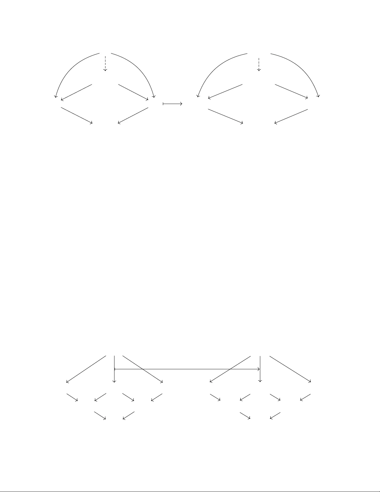
A COMPOSITIONAL FRAMEW ORK F OR CLASSICAL KINEMA TIC SYSTEMS ANDREA ABEJE-STINE AND D A VID WEISBAR T Dep artment of Mathematics University of California, Riverside Abstract. Our aim is to in tro duce a category-theoretic framew ork sufficiently general to describ e a wide v ariet y of op en kinematic systems in classical mechanics while uniquely c haracterizing systems with sp ecified simplest comp onen ts. The framework mo dels op en systems as morphisms in a category Kin ( F ), where comp osition enco des relationships b e- t ween subsystems and their em bedding into larger systems. Unlik e previous approac hes, the framew ork supp orts a precise treatment of geometric constrain ts, enabling the characteriza- tion of systems with feedback. A consequence is a structural formulation of low er kinematic pairs that clarifies system in teractions. Contents 1. In tro duction 1 2. Comp osition of systems 4 3. A CM-diagrams and their F -limits 9 4. The rigid inclusion category 29 5. Op en CMK systems as rigid inclusions 36 References 53 1. Intr oduction An open system is one that can in teract with external systems, and its description m ust accoun t for how it embeds into larger systems. A comp ositional approach to the study of op en systems asserts that the rules go v erning subsystem comp osition, together with the prop erties of the subsystems, determine the prop erties of the whole. This w ork develops a comp ositional framew ork for op en kinematic systems in classical mec hanics. Although mo deling in classical mechanics usually b egins with a configuration space and then imp oses constraints on it, the data describing a system is lo cal: comp onen ts interact only through constrain ts inv olving small collections of parts. The existence of a global con- figuration space is therefore not automatic but a compatibility question: does the collection of lo cal in teraction data determine a consisten t global configuration space? The results of this pap er show that, under natural lo cality assumptions, a configuration space exists if the constrain t data decomposes, and in that case it appears as a rigid univ ersal ob ject determined en tirely by the interactions. Theorem 4.1 iden tifies configuration spaces E-mail addr ess : astin005@ucr.edu, weisbart@math.ucr.edu . with F –limits ov er ACM-diagrams and establishes rigidit y , and Theorem 4.4 gives an exis- tence criterion by reducing general systems to decomp osing diagrams. When compatibilit y fails, lo cally sp ecified in teraction data need not assem ble in to a global configuration space; explicit examples exhibit this phenomenon (Examples 1 and 10 ). The ACM framework pro- vides a minimal structure needed to form ulate and pro v e classical non–existence results for kinematic pairs (Theorems 5.3 , 5.4 , and 5.5 ). The framework also serves as a foundation for subsequen t w ork on dynamics. A cen tral program in applied category theory inv olv es modeling op en systems as mor- phisms in a category , with comp osition encoding subsystem comp osition. This p ersp ectiv e originates in extended top ological quantum field theory , where cob ordism comp osition as- sem bles manifolds [ 5 , 9 , 14 , 20 ]. Subsequent work applies this approac h to electrical circuits [ 4 ], dynamical systems [ 37 ], and cyb er-physical systems [ 7 ]. In their study of classical me- c hanical systems, Baez et al. introduced a span-based framew ork for certain Lagrangian and Hamiltonian systems [ 6 ]. F or now, view a span in a category C to b e a pair of morphisms in C that ha v e the same source. The essential idea of Baez et al. w as to iden tify an op en classical mec hanical system with a span S in a category C [ 6 ]. The source of the morphisms that define S enco des the tra jectories of the system. Span comp osition determines how systems comp ose to form larger systems. Section 2 reviews the technical obstructions that arise when constructing span categories for classical mec hanical systems. These obstructions complicate direct application of existing op en-system framew orks [ 11 ]. The principal difficulty is that the relev an t categories do not admit pullbac ks. Baez et al. addressed this issue using generalized span categories [ 39 ]. Street introduced the notion of a fake pul lb ack to treat span categories in categories without pullbac ks [ 38 ]. The present work adopts the generalized span framew ork, whic h pro vides a direct extension of earlier work [ 39 ]. Street’s approach offers an alternative treatment of span comp osition in this setting, and its applicabilit y here merits further in vestigation. The framew ork in tro duced by Baez et al. [ 6 ] treats systems constructed from finitely man y linearly ordered subsystems. A spring–mass system consisting of finitely many masses constrained to mov e along a line and connected by springs pro vides a basic example. Suc h a system lo oks lik e this: F or a system with three masses and t w o springs, iden tifying the right mass of the left sub- system with the left mass of the righ t subsystem yields the larger system: F rom the Hamiltonian p ersp ectiv e, the state space of eac h mass is T ∗ R , the cotangent bundle of R . Eac h arrow in the diagram represents a canonical pro jection b et w een these subsystem state spaces: 2 T ∗ R T ∗ R T ∗ R 2 T ∗ R T ∗ R T ∗ R 2 T ∗ R 2 × T ∗ R T ∗ R 2 The canonical pro jections are surjective Poisson maps b etw een symplectic manifolds. The t w o spring–mass subsystems in the middle of the diagram ha v e state space T ∗ R 2 . The state space of the total system, describing three masses interacting in series, is the fib ered pro duct of tw o copies of T ∗ R 2 o v er T ∗ R . F rom the Lagrangian p ersp ectiv e, tangent bundles serv e as the state spaces, and the maps are surjectiv e Riemannian submersions. The fib ered pro duct mo dels the iden tification of the righ t mass of the left spring–mass system with the left mass of the righ t spring–mass system and yields a six-dimensional manifold rather than the eigh t-dimensional Cartesian pro duct of the subsystem state spaces. The use of fib ered products in this con text goes bac k at least to Dazord [ 12 ], who constructed configuration and state spaces for certain geometrically constrained systems in this wa y . Marle subsequen tly describ ed a broader class of constrained systems as submanifolds of unconstrained configuration or state spaces; in the holonomic case considered here, his results agree with those of Dazord [ 28 ]. The earlier framew ork [ 39 ] do es not accommo date systems with feedbac k or m ultiple geometric constrain ts. The follo wing system, in which three springs mediate interactions among three masses mo ving in R 2 , exhibits feedbac k not captured b y that framework: Although extensions of the earlier framework accommo date certain systems with feedback, the framew ork do es not directly describ e more complex systems suc h as link ages. The study of mechanical link ages is ancient; mec hanisms suc h as the trammel of Archimedes date bac k at least to Proclus and p ossibly to Arc himedes himself [ 40 ]. In 1875, F ranz Reuleaux articulated the comp ositional viewp oin t cen tral to the presen t w ork [ 35 ]: The elementary parts of a machine are not single, but o ccur alwa ys in pairs, so that the machine, from a kinematic p oint of view, m ust b e divided rather in to pairs of elemen ts than into single elements. Gr ¨ ubler formalized a mobilit y formula for planar link ages in 1917 [ 19 ], and Kutzbac h ex- tended it to spatial link ages in 1929 [ 25 ]. F reudenstein dev elop ed an efficient parameteriza- tion of four-link mec hanisms [ 17 ], building on earlier work of Burmester [ 10 ]. Denavit and Harten b erg in tro duced co ordinate parameterizations for comp osing constraint equations, in- cluding closed-lo op systems [ 13 ]. Mruthyunja ya dev elop ed a computational approach to the structural synthesis of link ages corresp onding to arbitrary graphs [ 33 ]. The study of link ages in tersects with algebraic geometry [ 29 ] and Lie theory [ 34 ], with connections reac hing bac k to Kempe’s Univ ersalit y Theorem [ 24 ] and to screw theory [ 8 ]. Kap o vic h and Millson studied the top ology of mo duli spaces of polygons and applied their study to link ages [ 22 , 23 ]. 3 The present w ork in tro duces a comp ositional framework for the kinematic study of a broad class of op en systems in classical mec hanics. The cen tral idea behind the framew ork of actor- constrain t mediated systems dev elop ed here is that the idealization of actors as p oint particles loses too m uc h information to supp ort a more precise comp ositional treatmen t. Actors may still b e represen ted as p oin t particles but ma y also carry internal information—or in ternal degrees of freedom—that enco de geometric constraints b et w een distinct actors. The frame- w ork establishes an abstract foundation for the study and classification of low er kinematic pairs in classical mec hanics. Examples clarify the structure of the framework and illustrate its relation to ph ysical in tuition. The framew ork explains ho w low er kinematic pairs com bine to form more complicated link ages and clarifies the conceptual basis of standard engineering classifications. No existing w ork formulates link age comp osition through (generalized) span comp osition in a setting that admits feedbac k. The actor-index categories and A CM-diagrams defined here resem ble the constraint graphs studied in constrain t satisfaction problems, b eginning with the w ork of F riedman and Leondes [ 15 , 16 ]. Recen t w ork mo dels constraint h yp ergraphs categorically [ 32 ]. Unlik e constraint h yp ergraphs of sets, ACM-diagrams encode the structure of the target category and satisfy more restrictiv e axioms. A CM-diagrams also resemble the construction of D -categories [ 2 ]. The relationship b etw een a constraint sk eleton and its asso ciated A CM-diagram resembles the functor I C : SimpGph → Quiv [ 30 ]. A k ey distinction is that D -categories and the functor I C provide structure for diagrams of actors and constrain ts, whereas the presen t framework also requires pairwise in teractions b et ween actors. The assembly of interactions in an A CM- diagram resembles op eradic comp osition in a m ulticategory [ 26 ], and the notion of op enness resem bles the study of net works using props [ 4 ]. Section 2 reviews earlier w ork on op en systems [ 6 ] and identifies its limitations for systems with feedbac k. It also presen ts the assumptions ab out kinematic systems in classical me- c hanics that motiv ate the introduction of a rigid inclusion category of ACM-systems . Giv en categories C and C ′ and a functor F : C → C ′ , Section 3 defines ACM-diagrams and formu- lates technical conditions on F related to the span-tigh tness condition [ 39 ]. It pro ves the results required for Section 4 . Section 4 introduces ACM-systems and their comp osition in a rigid inclusion category and prov es that the conditions from Section 3 yield an ACM-system unique up to isomorphism. T ake Diff to b e the category of smo oth manifolds with smo oth maps, and SurjSub to b e the category of smo oth manifolds with surjectiv e submersions. Section 5 sho ws that the forgetful functor F : SurjSub → Diff satisfies the conditions in tro duced in Sections 3 and 4 , yielding an ACM-category ov er F . It presen ts examples of op en kinematic systems in this framew ork and shows that certain link ages, although constructible from low er kinematic pairs, require more than tw o actors. In particular, it pro ves that the universal join t and the sliding hinge are not lo wer kinematic pairs b ecause they require at least three distinct actors. The section also initiates a classification of low er kinematic pairs. This classification arises naturally within the abstract framew ork and illustrates its applicabilit y to classical mec hanics. The emergence of an A CM-category in this setting indicates p ossible applications b ey ond classical mec hanics. 2. Composition of systems An actor in a classical mec hanical system, henceforth a CM-system, is a point particle with p ositive mass. Simple mo dels inv olve a finite collection of actors and their pairwise 4 in teractions. The state space of each actor is an ob ject in a category C that Section 5 sp ecifies. The dev elopment pro ceeds abstractly to construct a comp ositional framew ork for actor–constrain t mediated systems (ACM-systems). A kinematic system in classical mec hanics, henceforth a CMK system, is an ACM-system in whic h F : SurjSub → Diff is the forgetful functor from the category of surjectiv e submersions b et w een smo oth manifolds to the category of smo oth functions b et w een smo oth manifolds (Definition 5.1 ). 2.1. Constrain t skeletons of systems. The diagrammatic structure of classical mec hanics motiv ates the following notion. Informally , the c onstr aint skeleton of an ACM-system is a finite undirected graph (see Definition 4.3 for the formal definition). As an example, consider actors A , B , C , and D moving in three-dimensional Euclidean space. A massless rigid bar constrains B to mo ve on a sphere cen tered at the p osition of A . Actors C and D hav e no geometric constrain ts. Springs connect the pairs ( A, D ), ( B , C ), and ( C , A ), eac h applying a force along the line joining the tw o actors. The following graph represents the interactions of this A CM-system: A B C D The v ertices corresp ond to actors; the edges represen t elementary inter actions —those b e- t w een exactly t w o actors. These ma y b e geometric constrain ts or dynamical in teractions (i.e. forces). In the kinematic description of a CM-system, henceforth a CMK system, only the geometric constrain ts app ear. Th us, the ab o v e graph reduces to a constrain t skeleton like this: A B C D The goal is to define an abstract op en CMK system in a comp ositional framework that uniquely determines the state space from a collection of elementary inter actions —CMK sys- tems with tw o actors. The general framew ork go verns op en A CM-systems. Comp ositionalit y requires that the mo del of the total system b e constructed in finitely man y steps b y incor- p orating one elementary in teraction at a time. Each step dep ends only on the data of the in teracting pair of actors. The resulting mo del m ust b e indep endent of the order in whic h the elemen tary in teractions are included. 2.2. Comp ositional description of linearly-ordered systems. F or any categories J and C , a diagr am of shap e J in C is a functor D : J → C . The diagram D is finite if J is finite. The category J is an index c ate gory for diagrams in C with shap e J . This work restricts index categories to finite p osets. Consequen tly , J is thin. An y diagram D : J → C is therefore a comm utativ e diagram in C . A sp an S and a c osp an C in C are diagrams in C with shap e determined by three distinct ob jects { A, L, R } . A span assigns morphisms from A to L and from A to R , where a cospan assigns morphisms from L to A and from R to A , like this: 5 A L R and L R A Denote b y s L : S A → S L and s R : S A → S R the images of the left and righ t arro ws, resp ec- tiv ely , in C . The ob jects S L and S R are, resp ectiv ely , the left fo ot and right fo ot of S , and S A is the ap ex of S . When more careful sp ecification is needed, write S = ⟨ s L , s R ⟩ . Similarly , define c L : C L → C A and c R : C R → C A to b e the images of the arro ws in C , and write C = ⟩ c L , c R ⟨ . F or any spans S and Q with the same feet, a sp an morphism from S to Q is a morphism Φ in C from S A to Q A with s L = q L ◦ Φ and s R = q R ◦ Φ , so that this diagram comm utes: S A S L = Q L S R = Q R Q A s L s R Φ q L q R A span morphism Φ is a sp an isomorphism if Φ is an isomorphism. Denote by [ S ] the isomorphism class of spans isomorphic to S . A span Q is p air e d with a cospan C if Q L = C L , Q R = C R , and c L ◦ q L = c R ◦ q R . It is a pul lb ack of C if, in addition, the following univ ersal prop ert y holds: F or an y span S paired with C , there exists a unique span morphism Φ in C from S to Q . Comm utativity of these diagrams expresses the pairing and univ ersal prop erties of a pullbac k: Q A S A S A S L S R and S L S R C A C A ∃ ! F or any spans S and Q , if S R is equal to Q L and P A is a pullback of the cospan ⟩ s R , q L ⟨ , define S ◦ P Q = ⟨ s L ◦ p L , q R ◦ p R ⟩ 6 to be the span formed from morphisms in the left-hand diagram and equal to the span sho wn on the righ t: P A S A Q A P A S L S R = Q L Q R S L Q R The uniqueness of pullbacks of cospans up to span isomorphism defines a pro cedure for comp osing spans. Pullbacks of cospans, ho w ev er, do not necessarily exist in a category—and fail to exist in the categories most relev ant to the study of CM-systems. This motiv ates a generalization of the pullbac k concept. T ak e C ′ to b e an y category and F : C → C ′ to b e a functor. F or any span S and cospan C , the image F ( S ) is a span in C ′ , and F ( C ) is a cospan in C ′ . Definition 2.1. F or an y cospan C in C , a span S in C is an F -pul lb ack of C if F ( S ) is a pullbac k of F ( C ). This diagram illustrates the relationship b et w een S , C , F ( S ), and F ( C ) when S is an F -pullbac k of C : Q A S A F ( S A ) S L S R F ( S L ) F ( S R ) C A F ( C A ) ∃ ! F The functor F maps each morphism α in the span S to a morphism F ( α ) in the span F ( S ). Definition 2.2. The category C has F -pul lb acks if every cospan in C admits an F -pullback. A closely related concept is that of an F -pro duct and of C ha ving F -pro ducts. Define an F -pr o duct as an F -pullbac k ov er a terminal ob ject. Since the pullback of a cospan with morphisms into a terminal ob ject is a pro duct, if C has F -pullbacks and a terminal ob ject, and if F preserves terminal ob jects, then C has F -pro ducts. If F is the iden tit y functor and S is an F -pullback of a cospan C , then S is a pullbac k of C . The notion of an F -pullbac k th us generalizes the standard notion of a pullback. F or an y ob jects A , B , and C in C with morphisms f : A → C and g : B → C , if C is the category Set , then the fib er pro duct A × C B is the set A × C B =  ( a, b ) ∈ A × B | f ( a ) = g ( b )  . It is a pullback of ⟩ f , g ⟨ , and if F is the identit y functor on Set , then it is also an F -pullbac k of ⟩ f , g ⟨ . Contin ue to write A × C B for the apex of an F -pullback of ⟩ f , g ⟨ , and write A × B 7 when C is terminal (so f and g are unique). In the latter case, A × B is an F -product and the morphisms from it to A and B are F -pro jections. Prior work restricted the notion of span-tigh tness to functors F whose source category admits F -pullbac ks [ 39 ]. This condition can b e dropp ed. Definition 2.3. A functor F : C → C ′ is sp an-tight if for an y cospan C in C , and for ev ery pair of F -pullbac ks S and Q of C , the unique span morphism Φ from F ( S ) to F ( Q ) is of the form F (Ψ) for some Ψ in C . F or any spans S and Q in C so that S R is equal to Q L and ⟩ s R , q L ⟨ has an F -pullback P , the comp osite [ S ] ◦ [ Q ] is the span [ ⟨ s L ◦ p L , q R ◦ p R ⟩ ]. Comp osition, when defined, dep ends neither on the choice of represen tativ es S and Q , nor on the choice of F -pullbac k P . F or an y ob ject X in C , denote by Id X the identit y arrow with source and target equal to X . Iden tify S R as the source of [ S ] and S L as the target of S . Theorem 2.1 is a main result of the prior w ork [ 39 , Theorem 5.1]. Theorem 2.1. If C has F -pul lb acks and is sp an-tight, then ◦ defines c omp osition in a c ate gory Span ( F ) whose obje cts ar e the obje cts of C , whose morphisms ar e isomorphism classes of sp ans in C , and whose identity morphism at any obje ct X is [ ⟨ Id X , Id X ⟩ ] . F or appropriate c hoices of C and F , the prior w orks iden tify op en systems with morphisms in Span ( F ) (formerly denoted Span ( C , F )) [ 6 , 39 ], but this means that the sk eleton of any op en system with a connected sk eleton is an acyclic c hain, like this: Systems that cannot b e expressed as an acyclic chain as ab o v e cannot be constructed in Span ( F ) since the comp osition of morphisms can only pro ceed linearly . A c one Φ X o v er a diagram D : J → C is an ob ject X in C , the ap ex of the cone, together with c omp onent morphisms ( le gs ) Φ X Z : X → D ( Z ) for eac h ob ject Z in J suc h that for an y morphism f : A → B in J , D ( f ) ◦ Φ X A = Φ X B . A span paired with a cospan in C is a cone o ver that cospan. F or an y diagram D : J → C and an y ob jects X and Y in C , tak e Φ X and Φ Y to be cones o v er D . A morphism Ψ : X → Y is a c one morphism if for every ob ject A in J , Φ X A = Φ Y A ◦ Ψ . A cone morphism Ψ is a c one isomorphism if Ψ is an isomorphism in C . Cones Φ X and Φ Y are c one isomorphic if there exists a cone isomorphism from Y to X . A limit Φ X of a diagram D is a cone ov er D with the prop erty that for any cone Φ Y o v er D , there exists a unique cone morphism Ψ : Φ Y → Φ X . As in the case of spans, limits are to o restrictiv e for the categories relev an t here. This motiv ates the in tro duction of F -limits, whic h generalize F -pullbacks. Indeed, when F is the iden tit y functor on C , an F -limit is a limit. If C is the category Set , then the ap ex of a limit of a small diagram D : J → C is isomorphic to    x ∈ Y j ∈ Ob( J ) D ( j )      ∀ [ f : i → j ] ∈ Mor( J ) , D ( f )( π i ( x )) = π j ( x )    . See the textb o ok of Leinster for further discussion of this construction [ 27 ]. 8 Definition 2.4. F or an y t w o categories C and C ′ and functor F from C to C ′ , an F -limit of a diagram D is a cone Φ o v er D so that F (Φ) is a limit in C ′ of F ◦ D . Giv en an y index set I , category C , ob jects C i in C for each i in I , ob ject A in C , and any set of morphisms F = { f i : A → C i | i ∈ I } in C , the set F defines a cone ov er the discrete diagram formed b y the collection C i . If there is an F -pro duct P of the collection C i (equiv alently , an F -limit of the discrete diagram D from I to the collection C i ), then an F -pro duct morphism × i ∈ I f i : A → P is a cone morphism from A to P . This mak es precise what it means for A to factor through a pro duct when a pro duct does not exist, but an F -pro duct do es. T echnical issues arise in the construction of a category that has subsystem inclusions as its morphisms, namely the existence of certain F -limits and uniqueness up to isomorphism of the source of such F -limits. These issues motiv ate some restriction on both F and on the system of actors to b e studied. Definition 2.5. A functor F : C → C ′ is c one-tight if for every diagram D : J → C and every pair of F -limits Φ X and Φ X ′ of D , the unique cone isomorphism Ψ : F ( X ) → F ( X ′ ) from the cone F (Φ X ) to the cone F (Φ X ′ ) is F ( e Ψ) for some cone isomorphism e Ψ : X → X ′ . If F is cone-tight and preserv es terminal ob jects whic h C and C ′ ha v e, then F is span-tight. An y finite limit can be constructed b y pullbac ks [ 36 , Section 3.4]. The question is whether this is also true for F -limits with resp ect to F -pullbacks. In general, the answer is no (see Example 1 ), whic h complicates the presen t w ork. The goal of the next section is to identify a structured class of diagrams for whic h F -limits exist. 3. A CM-diagrams and their F -limits The central construction of this section is the A CM-diagr am . Lemma 3.5 provides the principal tec hnical ingredien t in proving that F -limits exist for A CM-diagrams that are r e ducible to de c omp osable by welding actors. 3.1. A CM-diagrams and weldings. Adding data that sp ecifies how parts connect allows comp osites b ey ond those arising from CM-systems with acyclic skeletons. Section 5 justifies this requiremen t and explains its implications for classical kinematics. Fix categories C and C ′ and a functor F : C → C ′ suc h that C admits F -pullbacks in C ′ . Assume that C and C ′ admit terminal ob jects and that F preserves them. Definition 3.1. An actor index c ate gory J is a finite p oset whose set of ob jects decomp ose as union Ob( J ) = Ob A ( J ) ∪ Ob C ( J ) ∪ Ob I ( J ) , where Ob A ( J ), Ob C ( J ), and Ob I ( J ) are disjoin t sets and (i) for some N in N , Ob A ( J ) is a set of N distinct elemen ts called actor indic es ; (ii) for each actor index i , there is an M i in N and a set C i of c onstr aint indic es for i with C i = { c i 1 , . . . , c i M i } ⊆ Ob C ( J ) 9 that all con tain a single distinguished ob ject  , and Ob C ( J ) = [ i ∈ Ob A ( J ) C i ; (iii) the set of inter action indic es is the set Ob I ( J ) = {{ i, j } | i, j ∈ Ob A ( J ) , i  = j } . The order is generated b y c ≤ i and i ≤ { i, j } for ev ery c in C i and for ev ery pair of distinct actor indices i and j . Definition 3.2. An A ctor-Constr aint me diate d diagr am D (henceforth an ACM-diagr am ) is, for some actor index category J , a diagram of shap e J in C with the following sp ecified prop erties: (i) D tak es each actor index i to an ob ject A i in C , called an actor , and eac h constraint index c in C i to an ob ject in C , called a c onstr aint for A i . (ii) D takes each morphism c ≤ i to a c onstr aint morphism f i,c : A i → D ( c ). (iii) D takes  to a terminal ob ject in C and D takes no other ob ject in J to a terminal ob ject in C . (iv) F or an y actors A i and A j with i and j distinct, there are F -pro duct morphisms × c ∈ C i ∩ C j f i,c : A i → Y c ∈ C i ∩ C j D ( c ) and × c ∈ C i ∩ C j f j,c : A j → Y c ∈ C i ∩ C j D ( c ) . (v) F or an y tw o distinct i and j , the functor D takes the span with source { i, j } and targets i and j to an F -pullback K ( A i , A j ) of the cospan giv en by the pair of mor- phisms × c ∈ C i ∩ C j f i,c : D ( i ) → Y c ∈ C i ∩ C j D ( c ) and × c ∈ C i ∩ C j f j,c : D ( j ) → Y c ∈ C i ∩ C j D ( c ) . Although the current work do es not require condition (v) in the definition of an ACM- diagram, it app ears to b e necessary for dynamics, where additional information such as a c hoice of p oten tial dep ends on pairs of actors rather than on individual actors. Definition 3.3 (Constrained actor) . A c onstr aine d actor A i with c onstr aint set Con( A i ), giv en b y a pair ( A i , Con( A i )), is an ACM-diagram A : J → C where J is an actor-index category with a single actor index i . There exists a finite index set K and ob jects B k of C for eac h k ∈ K such that Con( A i ) = { f i,k : A i → B k | k ∈ K } is a non-empt y set of morphisms. Refer to Con( A i ) as the c onstr aint set of A i . Each f i,k is a c onstr aint morphism . Ev ery actor considered in this work is a constrained actor. Accordingly , adopt the con- v en tion of writing A i for b oth the actor and the constrained actor ( A i , Con( A i )). Define the set of constrain ts of a diagram D b y Con( D ) =  D ( c ≤ a )   a ∈ Ob A ( J ) , c ∈ Ob C ( J ) , c ≤ a  . 10 F or an y category C , denote by Cat ↓ C the slice category whose ob jects are diagrams in C and whose morphisms are functors b et w een index categories that comm ute with those diagrams [ 18 , Section 2.5, Ex. 12], as illustrated here: J J ′ C F D D ′ Definition 3.4. F or an y categories J 1 and J 2 , an inclusion ι from J 1 to J 2 is a faithful functor ι : J 1  → J 2 that is injectiv e on Ob( J 1 ). In this case, J 1 is a sub c ate gory of J 2 . If J 1 and J 2 are actor index categories, then ι r esp e cts the ACM structur e if it sends actor indices to actor indices, constrain t indices to constrain t indices, in teraction indices to in teraction indices, and satisfies ι (  ) = . F or any diagram D 2 : J 2 → C , define (1) D 1 = D 2 ◦ ι. Denote by ι ∗ : D 1 → D 2 the induced morphism in Cat ↓ C . Call ι ∗ an inclusion of D 1 in to D 2 . If ι resp ects the ACM structure, then call ι ∗ an A CM sub diagr am of D 2 , and call D 1 an A CM sub diagr am of D 2 . An inclusion ι ∗ of A CM-diagrams that resp ects the ACM structure sends actor, constrain t, and interaction indices to actor, constrain t, and interaction indices. Since the F -pro duct morphisms and interactions for the target diagram exist in C , they also exist for the source diagram. A direct c heck of the definition of an A CM-diagram yields Lemma 3.1 . Lemma 3.1. If ι : J 1 → J 2 is an inclusion that r esp e cts the ACM structur e of actor index c ate gories J 1 and J 2 and D 2 : J 2 → C is an A CM-diagr am, then D 1 = D 2 ◦ ι is an ACM-diagr am. The w ay in which D 1 is a sub diagram of D 2 dep ends on the sp ecified inclusion. A sub dia- gram inclusion in v olv es only an inclusion functor from one actor index category to another, and this inclusion need not b e a set-inclusion. This has ph ysical significance: there ma y b e m ultiple wa ys in whic h a part could fit into a larger system; an inclusion is a choice of ho w that part fits in to the whole. An actor index category J is a finite p oset, and it mak es sense to iden tify a subset J ′ of J with the induced partial order. T ake J ′ to b e an actor index category suc h that Ob A ( J ′ ) ⊆ Ob A ( J ) , Ob C ( J ′ ) ⊆ Ob C ( J ) and Ob I ( J ′ ) = {{ i, j } | i, j ∈ Ob A ( J ′ ) , i  = j } . Denote by ι the set-inclusion functor J ′  → J that preserv es the partial order. The restriction D ′ = D | J ′ 11 is an A CM sub diagram of D . The category Cat of lo cally small categories, itself not lo cally small, has pullbac ks [ 36 , Prop osition 3.5.6]. Monomorphisms in Cat are the faithful functors that are injective on ob jects, hence they are the inclusions in Cat . In an y category , for any cospan ⟩ f , g ⟨ with pullbac k ⟨ ρ 1 , ρ 2 ⟩ , if f is a monomorphism then ρ 2 is a monomorphism [ 18 , Exercise 3.13.1]. A pullbac k of the inclusions ι 1 : J 1 → J and ι 2 : J 2 → J th us consists of a category J 12 and inclusions π 1 : J 12 → J 1 and π 2 : J 12 → J 2 . Definition 3.5. T ake D 1 and D 2 to b e sub diagrams of D , where D 1 : J 1 → C , D 2 : J 2 → C , D : J → C , and tak e ι 1 : J 1 → J and ι 2 : J 2 → J to b e the corresponding inclusions. An interse ction of sub diagr ams D 1 and D 2 in D consists of a pullbac k ⟨ π 1 , π 2 ⟩ with ap ex J 12 of the cospan ⟩ ι 1 , ι 2 ⟨ and a diagram D 12 : J 12 → C suc h that D 12 = D 1 ◦ π 1 = D 2 ◦ π 2 . Equiv alently , ⟨ π ∗ 1 , π ∗ 2 ⟩ is an F -pullbac k of ι ∗ 1 and ι ∗ 2 in Cat ↓ C . If D 1 and D 2 are ACM subdiagrams of D , then ⟨ π 1 , π 2 ⟩ is an interse ction of ACM sub di- agr ams in D . Call D 12 an interse ction of A CM sub diagr ams . If, in addition, Ob A ( J ) = ι 1  Ob A ( J 1 )  ∪ ι 2  Ob A ( J 2 )  and Ob C ( J ) = ι 1  Ob C ( J 1 )  ∪ ι 2  Ob C ( J 2 )  , then ⟩ ι 1 , ι 2 ⟨ is a union of ACM sub diagr ams o ver D 12 , and D is a union of ACM sub diagr ams D 1 and D 2 . In Set , the union of t wo sets is a pushout ov er the inclusions of their intersection. A union of ACM sub diagrams is not alwa ys a pushout in Cat ; rather, it is obtained by forming a pushout on the sub diagrams consisting of constraint s and actors and then constructing in teractions for eac h pair of actors. If C has F -pullbac ks, then a pushout of tw o A CM- diagrams determines an ACM-diagram whenev er the pushout satisfies condition 3.2 (iv), namely that for any tw o actors there exist F -pro duct morphisms into the F -pro duct of the constraints in the intersection of their constraint sets. Prop osition 3.1 shows that the graph-theoretic in tersection of ι 1 ( J 1 ) and ι 2 ( J 2 ) determines a pullbac k of A CM-diagrams. Prop osition 3.1. F or any ACM sub diagr ams D 1 and D 2 of D with inclusions on shap es ι 1 : J 1 → J and ι 2 : J 2 → J , an interse ction D 12 of D 1 and D 2 exists. If for every c in Ob C ( ι 1 ( J 1 ) ∩ ι 2 ( J 2 )) ther e exists an a in Ob A ( ι 1 ( J 1 ) ∩ ι 2 ( J 2 )) with c ≤ a , then D 12 is an ACM-diagr am, is isomorphic to ι 1 ( J 1 ) ∩ ι 2 ( J 2 ) , and is an ACM sub diagr am of b oth D 1 and D 2 . Pr o of. Since Cat has pullbac ks, the slice category Cat ↓ C has pullbac ks [ 36 , Prop osi- tion 3.3.8]. Hence an intersection D 12 of D 1 and D 2 exists. Define J 12 to b e the graph-theoretic in tersection of ι 1 ( J 1 ) and ι 2 ( J 2 ) inside J , namely , tak e Ob( J 12 ) = ι 1  Ob( J 1 )  ∩ ι 2  Ob( J 2 )  , 12 and tak e the morphisms of J 12 to b e the morphisms of J b et ween ob jects of J 12 . Comp osition and iden tities restrict from J , so J 12 is a sub category of J . F or i in { 1 , 2 } define π i : J 12 → J i as follows. F or eac h ob ject x of J 12 , since x is in ι i  Ob( J i )  and ι i is injectiv e on ob jects, there is a unique ob ject π i ( x ) of J i suc h that (2) ι i  π i ( x )  = x. F or an y morphism f : x → y in J 12 , since x and y are in ι i  Ob( J i )  and ι i ( J i ) is a sub category of J , the morphism f is in Hom ι i ( J i ) ( x, y ). Since ι i is faithful, there exists a unique morphism π i ( f ) : π i ( x ) → π i ( y ) in J i suc h that ι i  π i ( f )  = f . The functors π 1 and π 2 form a pullbac k of the cospan ⟩ ι 1 , ι 2 ⟨ in Cat . Giv en the h yp othesis on constraints in ι 1 ( J 1 ) ∩ ι 2 ( J 2 ), the category J 12 is an actor index category: all constrain t indices are asso ciated with actors; for any t w o actor indices in the in tersection, the interaction index b etw een those tw o actors is also in the in tersection; and it con tains  b ecause ι 1 and ι 2 preserv e the distinguished constrain t index  . Define the diagram D 12 : J 12 → C b y D 12 = D ◦ , where  : J 12  → J denotes the inclusion. Equiv alen tly , (3) D 12 = D 1 ◦ π 1 = D 2 ◦ π 2 . Equation 2 implies that the inclusions π i for i in { 1 , 2 } resp ect the A CM structure since eac h ι i resp ects the ACM structure. Since each π i resp ects the ACM structure, Lemma 3.1 implies that D 12 is an A CM-diagram, and ( 3 ) exhibits D 12 as an A CM sub diagram of b oth D 1 and D 2 . □ Comm utativit y of this diagram captures the data of Prop osition 3.2 : J 12 J ′ 12 J 1 J 2 J J ′ ϕ π 1 π 2 π ′ 1 π ′ 2 ι 1 ι ′ 1 ι 2 ι ′ 2 ψ Prop osition 3.2. F or any ACM-diagr ams D 1 : J 1 → C , D 2 : J 2 → C , D : J → C , and D ′ : J ′ → C such that D and D ′ ar e e ach unions of D 1 and D 2 with inclusions on shap es ι 1 : J 1 → J , ι 2 : J 2 → J , ι ′ 1 : J 1 → J ′ , and ι ′ 2 : J 2 → J ′ , 13 take ⟨ π 1 , π 2 ⟩ with ap ex J 12 to b e an interse ction (pul lb ack in Cat ) of the c osp an ⟩ ι 1 , ι 2 ⟨ , and ⟨ π ′ 1 , π ′ 2 ⟩ with ap ex J ′ 12 to b e an interse ction of ⟩ ι ′ 1 , ι ′ 2 ⟨ . If ther e exists an isomorphism of c ate gories φ : J 12 → J ′ 12 such that for i in { 1 , 2 } , π ′ i ◦ φ = π i , then ther e exists an isomorphism of c ate gories ψ : J → J ′ that r esp e cts the ACM structur e and a natur al isomorphism η : D → D ′ ◦ ψ . Pr o of. Define ψ : J → J ′ and ψ ′ : J ′ → J in the follo wing w ay: for any x in ι 1 ( J 1 ) and y in ι 2 ( J 2 ), tak e ψ ( x ) = ι ′ 1  ι − 1 1 ( x )  , ψ ( y ) = ι ′ 2  ι − 1 2 ( y )  , ψ ′ ( x ) = ι 1  ι ′− 1 1 ( x )  , and ψ ′ ( y ) = ι 2  ι ′− 1 2 ( y )  . If x is in ι 1 ( J 1 ) ∩ ι 2 ( J 2 ), then x = ι 1 ( π 1 ( z )) = ι 2 ( π 2 ( z )) for some z in J 12 . The equalities π ′ i ◦ φ = π i and ι ′ 1 ◦ π ′ 1 = ι ′ 2 ◦ π ′ 2 in J ′ 12 together imply that ι ′ 1  ι − 1 1 ( x )  = ι ′ 1  π 1 ( z )  = ι ′ 1  π ′ 1 ( φ ( z ))  = ι ′ 2  π ′ 2 ( φ ( z ))  = ι ′ 2  π 2 ( z )  = ι ′ 2  ι − 1 2 ( x )  , so the definition of ψ is consistent on the in tersection ι 1 ( J 1 ) ∩ ι 2 ( J 2 ). An equiv alen t argumen t v erifies that ψ ′ is also consisten t on this in tersection. Extend ψ and ψ ′ to in teraction indices b y ψ ( { a, b } ) = { ψ ( a ) , ψ ( b ) } and ψ ′ ( { a, b } ) = { ψ ′ ( a ) , ψ ′ ( b ) } . Since J and J ′ are posets whose orders are generated b y relations c ≤ a and a ≤ { a, b } , eac h of ψ and ψ ′ define an order-preserving map on ob jects and hence a functor. F or any x in J , there is an i in { 1 , 2 } such that x is in ι i ( J ), hence ψ ′ ◦ ψ ( x ) = ι i ( ι ′− 1 i ( ι ′ i ( ι − 1 i ( x )))) = x and ψ ◦ ψ ′ ( x ) = ι ′ i ( ι − 1 i ( ι i ( ι ′− 1 i ( x )))) = x. The functors ψ ′ and ψ are inv erses, hence ψ is an isomorphism. The isomorphism ψ resp ects actor, constrain t, and in teraction indices, and sends  to  . Define a natural transformation η : D → D ′ ◦ ψ comp onen t wise. (1) F or an y x in ι 1 ( J 1 ), D ( x ) = D 1 ( ι − 1 1 ( x )) and D ′ ( ψ ( x )) = D ′  ι ′ 1 ( ι − 1 1 ( x ))  = D 1 ( ι − 1 1 ( x )) , so tak e η x = id D ( x ) . Define ι 2 ( J 2 ) similarly for an y x in ι 2 ( J 2 ). (2) If x is an in teraction index { a, b } with a in ι 1 ( J 1 ) and b in ι 2 ( J 2 ), then D ( x ) and D ′ ( ψ ( x )) are (by the ACM-diagram axioms) c hosen F -pullbac ks of the same cospan in C , b ecause η is already the iden tit y on the actor ob jects and on the shared- constrain t pro ducts. The universal prop ert y of pullbac ks implies that there exists a unique isomorphism η x : D ( x ) ∼ = − → D ′ ( ψ ( x )) 14 that comm utes with the pullbac k pro jections. Because the index categories are thin, these c hoices automatically satisfy naturality once they comm ute with the structure maps (in particular, the pro jection maps in to the actor ob jects and shared-constrain t pro ducts). Th us η is a natural isomorphism. □ T ake J to b e an y actor index category and i to b e in Ob A ( J ). The c omplementary c onstr aint set to i is the set C ⊥ i, J = [ j  = i C j . This is the set of all constraint indices for actor indices in Ob A ( J ) other than i . The external c onstr aint set of i is the set Ext[ i : J ] = C i ∩ C ⊥ i, J , whic h may be empty and consists of all constraint indices in v olving b oth i and at least one actor index distinct from i . The set Ext[ i : J ] and the mappings to it capture the connection of the actor A i to the subsystem obtained b y excluding A i . T ake ι : J ′ → J to b e an inclusion that resp ects the ACM structure of another actor index category J ′ . The c onstr aint set of J ′ is the set C J ′ = [ j ∈ ι (Ob A ( J ′ )) C j . This is the set of all constraint indices in J inv olving at least one actor index in ι ( J ′ ). The set C J ′ is not necessarily equal to ι (Ob C ( J ′ )) b ecause there ma y b e constraints for actors in ι ( J ′ ) that are not constrain ts in ι ( J ′ ). The c omplementary c onstr aint set to J ′ is the set C ⊥ J ′ , J = [ a j / ∈ ι (Ob A ( J ′ )) C j . This is the set of all constrain t indices for actor indices in J not in ι ( J ′ ). The set C ⊥ J ′ , J is not necessarily equal to Ob C ( J ) \ ι (Ob C ( J ′ )) b ecause actors in Ob A ( J ) \ ι (Ob A ( J ′ )) may hav e constrain ts in ι ( J ′ ). The external c onstr aint set of J ′ is the set Ext[ J ′ : J ] = C J ′ ∩ C ⊥ J ′ , J , whose elements are the constraint indices for constraints that are betw een at least one actor for an actor index in J ′ and one actor for an actor index that is not in J ′ . Definition 3.6. An ACM-diagram D de c omp oses external c onstr aints if for each actor A , there exists an F -pro duct morphism f i := × c ∈ Ext[ i : J ] f i,c : A i → Y c ∈ Ext[ i : J ] D ( c ) . There is an imp ortan t difference b etw een 3.2 (iv) and 3.6 . The former requires that for every pair of actors, eac h actor maps through a pro duct of those tw o actors’ shared constrain ts; the latter requires that every actor maps through an F -pro duct of all of its constrain ts that are shared with at least one other actor, whic h p oten tially is an F -pro duct of man y more constrain ts. 15 Definition 3.7. An A CM-diagram D de c omp oses into c onstr aints if for eac h actor index i with corresp onding actor A i := D ( i ) , there is an F -pro duct morphism × c ∈ C i D ( c ≤ i ) : A i → Y c ∈ C i D ( c ) whic h is also an isomorphism. Definition 3.8. T ake A i and A j to b e an y distinct actors in an A CM-diagram, and tak e C := Y c ∈ C i ∩ C j D ( c ) to b e the F -pro duct of their shared constraints. The welding of A i and A j is the actor K ( A i , A j ) (see Definition 3.2 (v)) with constraint set C i ∪ C j . Refer to K ( A i , A j ) as a welde d actor . T ake D to b e an y A CM-diagram with actor-index category J that con tains distinct actor indices i and j . Construct the actor-index category W i,j ( J ) b y: • replacing i and j with a single index ij ; • deleting the interaction index { i, j } and its arrows; • assigning ij the constrain t set C ij = C i ∪ C j ; • substituting ij for ev ery o ccurrence of i or j elsewhere. The actor index category W i,j ( J ) contains all actor indices of J except i and j , and instead con tains the w elded actor index ij . Definition 3.9. F or any ACM-diagram D with shap e J having actors A i and A j , D is r e ducible by welding A i and A j if there is an A CM-diagram D ′ on W i,j ( J ) so that D ′ and D agree on every actor index, constrain t index, and morphism common to J and W i,j ( J ), and where D ′ tak es: • the welded actor ij to A ij : = D ( { i, j } ) = K ( A i , A j ); • any constrain t morphism of the w elded actor c ≤ ij to D ′ ( c ≤ ij ) : = ( D ( c ≤ i ) ◦ D ( i ≤ { i, j } ) , c ∈ C i , D ( c ≤ j ) ◦ D ( j ≤ { i, j } ) , c ∈ C j ; • any interaction index { ij , k } to K ( A ij , A k ), an F -pullbac k of A ij and A k o v er the F -pro duct Q c ∈ C ij ∩ C k D ( c ), • any in teraction morphism of the w elded actor ij ≤ { ij, k } to the pro jection π ij : K ( A ij , A k ) → A ij . In this case write D ( i,j ) − − → D ′ to mean that the diagram D reduces b y w elding A i and A j to the diagram D ′ . 16 Example 10 sho ws that not ev ery ACM-diagram is reducible by w elding. Another actor A k ma y map through the pro duct of the constraints it shares with A i and through the pro duct of the constraints it shares with A j , but not through the product of the constrain ts that it shares with the w elded actor K ( A i , A j ). Definition 3.10. A chain of r e ductions of an A CM-diagram D to an A CM-diagram D ′ is a finite sequence of A CM-diagrams ( D i ) i ∈{ 1 ,...,n } suc h that D = D 1 and D ′ = D n , and for each i in { 1 , . . . , n − 1 } , the diagram D i +1 is a reduction of D i b y welding tw o actors of D i . Definition 3.11. An A CM-diagram D in C is r e ducible to a de c omp osable A CM-diagr am if it decomposes external constraints or if there is a c hain of reductions of D to D ′ suc h that D ′ decomp oses external constrain ts. In this case, the diagram D ′ is a de c omp osing r e duction of the diagram D . 3.2. F -limits of ACM-diagrams. T ec hnical issues arise in constructing a category whose morphisms are subsystem inclusions, namely the existence of an F -limit for a given ACM- diagram and uniqueness up to isomorphism of the ap ex of such an F -limit. These issues motiv ate restricting b oth F and the class of A CM-diagrams. Definition 3.12. F or an y diagram D : J → C and an y cone Φ S o v er D with ap ex S , define the c one diagr am of D with ap ex S to b e the extension D S : J S → C obtained as follo ws: • T ak e J S to hav e the same ob jects and morphisms as J , together with a new maximal ob ject s and a morphism x ≤ s for eac h ob ject x of J . • Require that D S | J = D , D S ( s ) = S, and for eac h ob ject x of J , tak e D S ( x ≤ s ) = Φ S x : D ( x ) → S. When Φ X is an F -limit cone o v er D , refer to D X as the F -limit diagr am of D with ap ex X . The comp onen t morphisms of Φ S form a cone o ver D if and only if the cone diagram D S is comm utativ e. Lemma 3.2. T ake F to b e a faithful functor and D to b e an ACM-diagr am. F or any c one Φ S over D , the c omp onent morphisms into actors uniquely determine Φ S . Pr o of. F or any distinct actor indices i and j in J , denote by Φ S i : S → A i the comp onen t morphism of the cone Φ S in to the actor A i and by Φ S ij the comp onen t morphism from S to K ( A i , A j ). This diagram represen ts the relev ant morphisms and ob jects: 17 D S S F ◦ D S F ( S ) K ( A i , A j ) F ( K ( A i , A j )) A i A j F ( A i ) F ( A j ) Q c ∈ C i ∩ C j D ( c ) F ( Q c ∈ C i ∩ C j D ( c )) Φ S ij Φ S i Φ S j F (Φ S ij ) F (Φ S i ) F (Φ S j ) π i π j F ( π i ) F ( π j ) f i F f j F ( f i ) F ( f j ) The diagram D S is comm utativ e so Φ S i = π i ◦ Φ S ij and Φ S j = π j ◦ Φ S ij . F unctoriality of F implies that (4) F (Φ S i ) = F ( π i ) ◦ F (Φ S ij ) and F (Φ S j ) = F ( π j ) ◦ F (Φ S ij ) . The span ⟨ π i , π j ⟩ is an F -pullback, so there is a unique cone morphism from F ( S ) to F ( K ( A i , A j )) that satisfies ( 4 ), hence F (Φ S ij ) is the unique morphism that satisfies ( 4 ). F aithfulness of F implies that Φ S ij is the unique morphism in C that F sends to F (Φ S ij ), so comp onen t morphisms in to interactions are determined b y the morphisms in to actors. The diagram D S comm utes, so the comp onen t morphism Φ S c in to an y constraint D ( c ) satisfies Φ S c = f i,c ◦ Φ S i for an y actor index i suc h that c is in C i . □ Definition 3.13. A functor F is sp an-extendable if whenev er the cospan ⟩ c L , c R ⟨ has an F -pullbac k ⟨ p L , p R ⟩ and the cospan ⟩ c L ◦ f , c R ◦ g ⟨ has an F -pullback ⟨ q L , q R ⟩ , the unique span morphism Φ from ⟨F ( f ◦ q L ) , F ( g ◦ q R ) ⟩ to ⟨F ( p L ) , F ( p R ) ⟩ is F (Ψ), where Φ : F ( Q A ) → F ( P A ) and Ψ : Q A → P A , P A is the ap ex of the F -pullback ⟨ p L , p R ⟩ , Q A is the ap ex of the F -pullback ⟨ q L , q R ⟩ , and Ψ is a span morphism. This diagram captures the meaning of the functor F b eing sp an-extendable : Q A F ( Q A ) Q L P A Q R F ( Q L ) F ( P A ) F ( Q R ) C L C R F ( C L ) F ( C R ) C A F ( C A ) q L Ψ q R F ( q L ) ∃ !Φ F ( q R ) f p L p R g F ( f ) F ( p L ) F ( p R ) F ( g ) c L c R F ( c L ) F ( c R ) F If C and C ′ b oth hav e terminal ob jects and F : C → C ′ preserv es terminal ob jects, then span-extendabilit y of F implies Lemma 3.3 b y taking C A to b e a terminal ob ject of C . 18 Lemma 3.3. If F is sp an-extendable, f : A → B and g : A ′ → B ′ ar e morphisms in C , and ⟨ π A , π A ′ ⟩ with ap ex A × A ′ and ⟨ π B , π B ′ ⟩ with ap ex B × B ar e F -pr o ducts, then ther e is a pr o duct morphism f × g : A × A ′ → B × B ′ in C . Lemma 3.3 establishes that a middle arrow in the following commutativ e diagram exists whenev er f and g exist: A A × A ′ A ′ B B × B ′ B ′ 1 f π A π A ′ f × g g π B π B ′ While F ( f ) × F ( g ) is the unique morphism that satisfies an equiv alent diagram to the ab o v e in C ′ , the morphism f × g is not necessarily unique in C without additionally assuming that F is faithful. Lemma 3.4. Supp ose that C and C ′ have terminal obje cts that F pr eserves. T ake S , Q , and T to b e obje cts in C with ⟨ p 1 L , p 1 R ⟩ an F -pr o duct of S and Q with ap ex S × Q , ⟨ p 2 L , p 2 R ⟩ an F -pr o duct of S × Q and T with ap ex ( S × Q ) × T , and ⟨ p 3 L , p 3 R ⟩ an F -pr o duct of Q and T with ap ex Q × T . If ⟨ p L , p R ⟩ is an F -pul lb ack of the c osp an ⟩ p 1 R , p 3 L ⟨ with ap ex ( S × Q ) × Q ( Q × T ) , then the fol lowing c ones over the discr ete diagr am on { S, Q, T } ar e isomorphic: ( S × Q ) × T with le gs  p 1 L ◦ p 2 L , p 1 R ◦ p 2 L , p 2 R  , ( S × Q ) × Q ( Q × T ) with le gs  p 1 L ◦ p L , p 1 R ◦ p L (= p 3 L ◦ p R ) , p 3 R ◦ p R  . The ob jects and morphisms in volv ed in Lemma 3.4 are arranged lik e this: ( S × Q ) × T ( S × Q ) × Q ( Q × T ) S × Q S × Q Q × T S Q T S Q T S R = Q L ∼ = 1 Q R = T L ∼ = 1 S R = Q L ∼ = 1 Q R = T L ∼ = 1 Φ p 2 L p 2 R p L p R p 1 L p 1 R p 1 L p 1 R p 3 L p 3 R s R q L q R t L s R q L q R t L Pr o of. Under the standing hypothesis that C and C ′ ha v e terminal ob jects that F preserves, prior w ork [ 39 , Lemma 5.4] constructs a span isomorphism Φ : ( S × Q ) × T → ( S × Q ) × Q ( Q × T ) b et w een the spans ⟨ p 1 L ◦ p 2 L , p 2 R ⟩ and ⟨ p 1 L ◦ p L , p 3 R ◦ p R ⟩ . Moreo v er, Φ is constructed as a span morphism ⟨ p 2 L , p 2 R ⟩ → ⟨ p L , p 3 R ◦ p R ⟩ , so in particular (5) p 2 L = p L ◦ Φ and p 2 R = ( p 3 R ◦ p R ) ◦ Φ . 19 It remains to show that Φ resp ects the Q -leg. Use the left equalit y of ( 5 ) to obtain the equalit y (6) p 1 R ◦ p 2 L = ( p 1 R ◦ p L ) ◦ Φ . Since ⟨ p L , p R ⟩ is an F -pullbac k of the cospan ⟩ p 1 R , p 3 L ⟨ , (7) p 1 R ◦ p L = p 3 L ◦ p R . Equations ( 6 ) and ( 7 ) together imply that p 1 R ◦ p 2 L = ( p 3 L ◦ p R ) ◦ Φ , so Φ is a cone morphism o v er { S, Q, T } . Since Φ is a span isomorphism (hence an isomor- phism in C ), it has an in v erse Φ − 1 , which by a similar argument is also a cone morphism, so the t w o cones are isomorphic. □ Apply Lemma 3.4 with the roles of S and T permuted to obtain a cone isomorphism ( S × Q ) × T ∼ = S × ( Q × T ) o v er the discrete diagram on { S, Q, T } . Thus F -pro ducts are asso ciative up to cone isomor- phism, so write S × Q × T . R emark. The conclusion of Lemma 3.4 do es not require terminal ob jects. The assumptions that C and C ′ ha v e terminal ob jects that F preserves allo ws the use of the prior work to pro vide an explicit span isomorphism Φ : ( S × Q ) × T → ( S × Q ) × Q ( Q × T ) that is already a cone isomorphism on the S - and T -legs. The pro of abov e only c hecks that Φ also resp ects the Q -leg. If A and B are t w o sets of ob jects in C , then Lemma 3.4 implies that there is a cone isomorphism (8) Y X ∈A∪B X ∼ = Y A ∈A A × Q Y ∈A∩B Y Y B ∈B B . Definition 3.14. A category C has nonde gener ate F -pullbacks if it has F -pullbacks, F preserv es terminal ob jects, and if for an y F -pullback P whose feet are not terminal ob jects, the ap ex of P is also not a terminal ob ject. Prop osition 3.3 is a statement ab out the existence of F -limits, namely , it is the formal statemen t that if a diagram is reducible to decomp osable, then that diagram has an F -limit. Pro ving Lemmata 3.5 and 3.6 are critical steps in pro ving Prop osition 3.3 . F or the remainder of this section, assume C has non-degenerate F -pullbacks and F is span-extendable and cone- tigh t. Lemma 3.5. F or any A CM-diagr am D : J → C with distinct actor indic es i 0 and j 0 , if D de c omp oses external c onstr aints, then it has a r e duction D ′ : W i 0 ,j 0 ( J ) → C obtaine d by welding A i 0 and A j 0 . Mor e over, D ′ is an ACM-diagr am that de c omp oses external c onstr aints. Preserv ation of the A CM-diagram structure under w elding requires the additional assump- tion of non-degeneracy of F -pullbac ks, hence the in tro duction of the new definition. 20 Pr o of. Decomp ose unions and int ersections to obtain the equalities Ext[ i 0 : J ] ∩ Ext[ j 0 : J ] =  C i 0 ∩ [ j  = i 0 C j  ∩  C j 0 ∩ [ j  = j 0 C j  =  C i 0 ∩  C j 0 ∪ [ j  = i 0 ,j 0 C j  ∩  C j 0 ∩  C i 0 ∪ [ j  = i 0 ,j 0 C j  =  C i 0 ∩ C j 0  ∪  C i 0 ∩ [ j  = i 0 ,j 0 C j  ∩  C i 0 ∩ C j 0  ∪  C j 0 ∩ [ j  = i 0 ,j 0 C j  =  C i 0 ∩ C j 0  ∪  C i 0 ∩ [ j  = i 0 ,j 0 C j  ∩  C j 0 ∩ [ j  = i 0 ,j 0 C j  =  C i 0 ∩ C j 0  ∪  C i 0 ∩ C j 0 ∩ [ j  = i 0 ,j 0 C j  = C i 0 ∩ C j 0 , hence (9) Ext[ i 0 : J ] ∩ Ext[ j 0 : J ] = C i 0 ∩ C j 0 . Similarly , Ext[ i 0 : J ] ∪ Ext[ j 0 : J ] =  C i 0 ∩ [ j  = i 0 C j  ∪  C j 0 ∩ [ j  = j 0 C j  =  C i 0 ∩ C j 0  ∪  ( C i 0 ∪ C j 0 ) ∩ [ b  = i 0 ,j 0 C b  = ( C i 0 ∩ C j 0 ) ∪ Ext[ i 0 j 0 : J ′ ] . (10) Equation ( 8 ) together with ( 9 ) and ( 10 ) implies that there is an F -pro duct isomorphism (11) Y c ∈ Ext[ i 0 : J ] D ( c ) × Q c ∈ C i 0 ∩ C j 0 D ( c ) Y c ∈ Ext[ j 0 : J ] D ( c ) ∼ − − → Y c ∈ Ext[ i 0 : J ] ∪ Ext[ j 0 : J ] D ( c ) . Define A i 0 j 0 to b e the ap ex of the in teraction K ( A i 0 , A j 0 ). Since F is span-extendable, there is an induced span morphism ψ : A i 0 j 0 → Y c ∈ Ext[ i 0 : J ] D ( c ) × Q c ∈ C i 0 ∩ C j 0 D ( c ) Y c ∈ Ext[ j 0 : J ] D ( c ) . Comp ose ψ with the isomorphism in ( 11 ) to obtain an F -pro duct morphism ˜ f i 0 j 0 : A i 0 j 0 → Y c ∈ Ext[ i 0 : J ] ∪ Ext[ j 0 : J ] D ( c ) . Denote b y J ′ the w elded index category W i 0 ,j 0 ( J ). Equation ( 10 ) implies that Ext[ i 0 j 0 : J ′ ] = ( C i 0 ∪ C j 0 ) ∩ [ b  = i 0 ,j 0 C b ⊆ Ext[ i 0 : J ] ∪ Ext[ j 0 : J ] , 21 and asso ciativity of F -pro ducts as a consequence of Lemma 3.4 determines an F -pro duct morphism π ∪ : Y c ∈ Ext[ i 0 : J ] ∪ Ext[ j 0 : J ] D ( c ) → Y c ∈ Ext[ i 0 j 0 : J ′ ] D ( c ) . Define (12) f i 0 j 0 := π ∪ ◦ ˜ f i 0 j 0 : A i 0 j 0 → Y c ∈ Ext[ i 0 j 0 : J ′ ] D ( c ) . This is the required F -pro duct morphism for the w elded actor. The equalit y Ext[ b : J ′ ] = Ext[ b : J ] together with the assumption that D decomp oses external constraints determines an F - pro duct morphism (13) f b : A b → Y c ∈ Ext[ b : J ′ ] D ( c ) . Finally , construct the in teraction b et w een A i 0 j 0 and A b . Since C i 0 j 0 ∩ C b is a subset of Ext[ i 0 j 0 : J ′ ], associativity of F -pro ducts as a consequence of Lemma 3.4 determines an F -pro duct pro jection Y c ∈ Ext[ i 0 j 0 : J ′ ] D ( c ) → Y c ∈ C i 0 j 0 ∩ C b D ( c ) , so f i 0 j 0 induces a morphism (14) A i 0 j 0 → Y c ∈ C i 0 j 0 ∩ C b D ( c ) . Similarly , since Ext[ b : J ′ ] = Ext[ b : J ] ⊇ C b ∩ ( C i 0 ∪ C j 0 ) = C b ∩ C i 0 j 0 , asso ciativit y of F -pro ducts as a consequence of Lemma 3.4 determines an F -pro duct pro- jection Y c ∈ Ext[ b : J ′ ] D ( c ) → Y c ∈ C i 0 j 0 ∩ C b D ( c ) , so f b induces a morphism (15) A b → Y c ∈ C i 0 j 0 ∩ C b D ( c ) . The in teraction K ( A i 0 j 0 , A b ) exists as an F -pullback of the cospan determined by the mor- phisms ( 14 ) and ( 15 ). Define D ′ : J ′ → C to b e a reduction of D b y w elding A i 0 and A j 0 . Every arrow of D ′ is either an arro w of D or a comp osite of such arro ws with pro jections from an F -pullback, so D ′ resp ects identities and comp osition. Since every in teraction K ( A i 0 j 0 , A b ) exists, D ′ is a w ell-defined functor. V erify the ACM conditions to sho w that D ′ is an ACM-diagram. Conditions (i) and (ii) of Definition 3.2 hold for D ′ b ecause they hold for D and the w elding do es not alter any part of the diagram aw ay from the new ob ject i 0 j 0 . Condition (v) holds b y construction of the new in teractions as F -pullbacks. Since C has nondegenerate F -pullbac ks and D sends no ob ject other than  to a terminal ob ject, the new apices in tro duced by welding and by the new 22 in teractions are not terminal, so (iii) holds for D ′ . Condition (iv) follows from items ( 14 ) and ( 15 ). Th us D ′ is an A CM-diagram. The construction of the morphisms ( 12 ) and ( 13 ) demonstrates that every actor of D ′ admits an F -pro duct morphism to the pro duct of its external constraints, so D ′ decomp oses external constrain ts. □ Lemma 3.6. T ake D to b e an ACM-diagr am that de c omp oses external c onstr aints of shap e J in C with actors A i and A j and take D ′ to b e a r e duction of D by welding A i and A j . If D ′ has an F -limit Φ L , then D has an F -limit Ψ L with identic al ap ex L so that for any x in b oth J and W i,j ( J ) , Ψ L x = Φ L x . F urthermor e, Ψ L i = ρ i ◦ Φ L ij and Ψ L j = ρ j ◦ Φ L ij wher e ⟨ ρ i , ρ j ⟩ is the sp an K ( A i , A j ) . Comm utativit y of this diagram captures the data of Lemma 3.6 : S L A ij k A ij A j k A i A j A k Φ Φ S ij k Φ S ij Φ S k Φ L ij k ρ ij ϕ j k ρ k Pr o of. T ak e ⟨ ρ i , ρ j ⟩ to b e the span K ( A i , A j ) with ap ex A ij . F or eac h actor index k that is not in { i, j } and each a in { i, j } , take ⟨ ρ ij , ρ k ⟩ := K ( A ij , A k ) and ⟨ ρ a , ρ k ⟩ := K ( A a , A k ) , with resp ectiv e apices A ij k and A ak . The morphism ρ a : A ij → A a and the iden tit y on A k determine a morphism of cospans from the shared-constraint cospan of ( A ij , A k ) to the shared-constrain t cospan of ( A a , A k ). Since F is span-extendable, this morphism of cospans induces a unique span morphism φ ak : A ij k → A ak satisfying comm utativit y with the pullback pro jections. Construct a cone Ψ L o v er D with ap ex L as follo ws. (1) If x is an ob ject of J that is also an ob ject of W i,j ( J ), set Ψ L x := Φ L x . (2) Define the actor legs Ψ L i := ρ i ◦ Φ L ij and Ψ L j := ρ j ◦ Φ L ij . 23 (3) F or eac h k not in { i, j } and eac h a in { i, j } , define the interaction leg Ψ L ak := φ ak ◦ Φ L ij k : L → A ak . Denote b y J ′ the category W i,j ( J ). F or an y cone Ψ S o v er F ◦ D with apex S , construct a cone Φ S o v er F ◦ D ′ with the same ap ex S as follo ws. (1) If x is an ob ject of J ′ that is also an ob ject of J , set Φ S x := Ψ S x . (2) Since F ( ⟨ ρ i , ρ j ⟩ ) is a pullback span and (Ψ S i , Ψ S j ) is paired with the shared-constraint cospan of ( A i , A j ), the pullbac k univ ersal prop ert y gives a unique morphism Φ S ij : S → F ( A ij ) suc h that F ( ρ i ) ◦ Φ S ij = Ψ S i and F ( ρ j ) ◦ Φ S ij = Ψ S j . (3) F or eac h k that is not in { i, j } , the pair (Φ S ij , Ψ S k ) is paired with the shared-constraint cospan of ( A ij , A k ), hence the pullbac k univ ersal prop erty of F ( ⟨ ρ ij , ρ k ⟩ ) giv es a unique morphism Φ S ij k : S → F ( A ij k ) whose comp osites with the t w o pullbac k pro jections are Φ S ij and Ψ S k , resp ectiv ely . T o c hec k that Φ S is a cone o v er F ◦ D ′ , take α to b e an y morphism α : x → y in J ′ . The cone condition is the equalit y F ( D ′ ( α )) ◦ Φ S x = Φ S y . If α lies in the part of J ′ inherited from J a w ay from the welded ob jects, then D ′ ( α ) = D ( α ) , Φ S x = Ψ S x , and Φ S y = Ψ S y , so the equality holds because Ψ S is a cone o v er F ◦ D . If α is one of the pro jection morphisms out of a pullback span defining A ij or A ij k , then the equalit y holds b y the defining identities for Φ S ij and Φ S ij k obtained from the corresp onding pullbac k univ ersal prop erties. Therefore Φ S is a cone o v er F ◦ D ′ . Since F (Φ L ) is a limit cone of F ◦ D ′ , there is a unique cone morphism Φ : S → F ( L ) from Φ S to F (Φ L ). The definitions of Ψ L in terms of Φ L imply that the equalities Φ S x = F (Φ L x ) ◦ Φ for all ob jects x of J ′ determine Ψ S y = F (Ψ L y ) ◦ Φ for ev ery ob ject y of J . Hence Φ is a cone morphism Ψ S → F (Ψ L ) o v er F ◦ D . If Φ ′ : S → F ( L ) is an y cone morphism Ψ S → F (Ψ L ) ov er F ◦ D , then the same verification on the generating morphisms of J ′ sho ws that Φ ′ is also a cone morphism Φ S → F (Φ L ) ov er F ◦ D ′ . Uniqueness of Φ o v er F ◦ D ′ implies Φ ′ is equal to Φ. Therefore F (Ψ L ) is a limit of F ◦ D , and so Ψ L is an F -limit of D . □ Prop osition 3.3. If D is a r e ducible to de c omp osable ACM-diagr am, then ther e is a chain of r e ductions of D to a diagr am D ′ wher e D ′ has one actor. F urthermor e, any A CM-diagr am that is r e ducible to a de c omp osable A CM-diagr am admits an F -limit in C which has an ap ex that isomorphic to the actor in D ′ . 24 Pr o of. F or any A CM-diagram H that decomp oses external constrain ts with exactly one actor index a and corresp onding actor A , Lemma 3.2 implies that cones ov er F ◦ H with ap ex S are in bijection with morphisms S → F ( A ). Therefore the iden tit y id F ( A ) : F ( A ) → F ( A ) determines a limit of F ◦ H , hence H admits an F -limit with ap ex A . T ake n to b e any natural num ber. Assume that ev ery ACM-diagram that decomp oses external constrain ts with n actor indices admits an F -limit. T ak e any ACM-diagram G n +1 that decomp oses external constrain ts with n + 1 actor indices. Cho ose distinct actor indices i and j of G n +1 and w eld them to obtain a reduction G n +1 → G n with n actor indices. Lemma 3.5 implies that G n decomp oses external constraints, so the inductiv e hypothesis gives an F -limit of G n . Lemma 3.6 then gives an F -limit of G n +1 with the same ap ex. This completes the induction, so ev ery ACM-diagram that decomp oses external constrain ts admits an F -limit. F or an y ACM-diagram D that is reducible to decomp osable, fix a c hain of decomp osing reductions D = D 0 → D 1 → · · · → D m =: E N , where E N decomp oses external constrain ts and has N actor indices. Repeatedly w eld actors to obtain a c hain of decomp osing reductions E N → E N − 1 → · · · → E 1 , where E 1 has exactly one actor index and corresp onding actor L . Since E 1 has only one actor index, it admits an F -limit with ap ex L . The c hain of weldings E N → E N − 1 → · · · → E 1 is finite, and Lemma 3.6 transp orts an F -limit along the chain in the direction opp osite to the arrows. Therefore E N admits an F -limit with ap ex L . The same reasoning applied to the c hain D = D 0 → D 1 → · · · → D m = E N yields an F -limit of D with apex L . □ Prop osition 3.4 pro vides the technical foundation for Theorem 4.2 , whic h shows how the framew ork of A CM categories p ermits the construction of larger systems from subsystems. In general, the union of ACM-diagrams may fail to exist b ecause a larger collection of actors could p oten tially inv olve additional constraints for eac h actor, and require mapping actors in to to o many constraints. Even if a union of tw o A CM-diagrams exists, the question remains: when do es that A CM-diagram hav e an F -limit? Both D 1 and D 2 decomp osing external constrain ts is not enough, as Example 1 shows. Prop osition 3.4. Supp ose that C has F -pul lb acks and take F to b e a c one-tight, faithful, sp an-extendable functor that pr eserves terminal obje cts. If D 1 and D 2 ar e A CM sub diagr ams of an ACM-diagr am D that de c omp oses into c onstr aints so that their interse ction D 12 is either: (1) A diagr am with no actors, or (2) An ACM sub diagr am of D 1 and D 2 such that for every actor a in D 12 , ι 1 ( C a ) = C ι 1 ( a ) and ι 2 ( C a ) = C ι 2 ( a ) , 25 and if D is their union over D 12 , then ther e ar e F -limits Φ X 1 1 , Φ X 2 2 , and Φ X 12 12 of D 1 , D 2 , and D 12 r esp e ctively. F urthermor e, ther e ar e F -pr o duct morphisms fr om X 1 to X 12 and fr om X 2 to X 12 with an F -pul lb ack which defines an F -limit of D . Pr o of. Lemma 3.4 implies that any ACM-diagram D ′ : J ′ → C that decomp oses in to con- strain ts has an F -limit that is cone isomorphic to the F -product of its actors. F or eac h i in { 1 , 2 } , tak e Φ X i i to b e the F -limit of D i with ap ex X i = Y c ∈ Ob C ( J i ) D ( c ) , whose legs are the unique morphisms that F tak es to the canonical pro jections to the actors and constrain t of F ◦ D i , together with the induced legs to the in teractions of F ◦ D i . Since eac h in teraction is an F -pullbac k and F is span-extendable, the pro jections to its actors determine a unique leg from X i . In case (1), the diagram D 12 has no actors, so it is discrete and admits an F -limit, namely the F -pro duct X 12 = Y c ∈ Ob C ( J 12 ) D ( c ) , with the unique morphisms in C that F tak es to the canonical pro jections. Henceforth abuse terminology b y referring to morphisms app earing in this w a y as canonical pro jections. In case (2), the diagram D 12 is an A CM sub diagram of D 1 and D 2 and the h yp otheses ι 1 ( C a ) = C ι 1 ( a ) and ι 2 ( C a ) = C ι 2 ( a ) ensure that ev ery actor of D 12 is isomorphic to the same F -pro duct of constrain ts as in D 1 and D 2 . Therefore D 12 decomp oses into constrain ts. T ake Φ X 12 12 as an F -limit of D 12 with ap ex the F -product X 12 = Y c ∈ Ob C ( J 12 ) D ( c ) , with the canonical pro jections to its actor and constrain t ob jects and induced legs to its in teraction ob jects. Since the construction of an F -limit Φ X 12 12 of D 12 in case (1) is identical to the construction in case (2), pro ceed in either case as follo ws. The con tainmen t Ob C ( J 12 ) ⊆ Ob C ( J i ) together with associativity of F -pro ducts as a consequence of Lemma 3.4 determine F - pro duct pro jections Ψ 1 : X 1 → X 12 and Ψ 2 : X 2 → X 12 . T ake ⟨ ρ 1 , ρ 2 ⟩ to b e an F -pullbac k of the cospan ⟩ Ψ 1 , Ψ 2 ⟨ with ap ex X . Define a cone Φ X o v er D on the actors, constrain ts, and interactions of either D 1 or D 2 as follo ws. F or an y ob ject x of J , if x lies in J i , then define Φ X x := Φ X i x ◦ ρ i : X → D ( x ) . T ake y to b e an y ob ject in J 12 . Since ⟨ ρ 1 , ρ 2 ⟩ is a pullbac k, Ψ 1 ◦ ρ 1 = Ψ 2 ◦ ρ 2 . 26 Comp ose eac h of these morphisms with the leg X 12 → D ( y ) to obtain Φ X 12 y ◦ Ψ 1 ◦ ρ 1 = Φ X 12 y ◦ Ψ 2 ◦ ρ 2 , Eac h Ψ i for i in { 1 , 2 } is an F -pro duct pro jection, so each are cone morphisms ov er D 12 . Th us, Φ X 1 y = Φ X 12 y ◦ Ψ 1 and Φ X 2 y = Φ X 12 y ◦ Ψ 2 and so Φ X 1 y ◦ ρ 1 = Φ X 2 y ◦ ρ 2 , whic h sho ws that Φ X y do es not dep end on the c hoice of i . T ake a and b to b e actor indices in J . Since D is an ACM-diagram,  is in C a for ev ery actor index a in J , hence  is in C a ∩ C b . If { a, b } lies in J 1 , define Φ { a,b } := Φ X 1 { a,b } ◦ ρ 1 : X → D ( { a, b } ) . If { a, b } lies in J 2 , define Φ { a,b } := Φ X 2 { a,b } ◦ ρ 2 : X → D ( { a, b } ) . Otherwise, one of a and b lies in J 1 and the other lies in J 2 . In this case, define Φ { a,b } directly from the already-defined legs to the t wo actors and to the shared constraints. Lemma 3.4 together with D decomp osing into constrain ts implies that D ( { a, b } ) is an F - pro duct Q c ∈ C a ∪ C b D ( c ). Since C a ∪ C b is a subset of Ob C ( J ), asso ciativit y of F -pro ducts as a consequence of Lemma 3.4 implies there is an F -pro duct pro jection Φ X { a,b } : X → D ( { a, b } ) suc h that p a ◦ Φ X i { a,b } = Φ X { a,b } and p b ◦ Φ X { a,b } = Φ X j b , where a is an ob ject of J i and b is an ob ject of J j . Since Φ X { a,b } is an F -pro duct pro jection, it is a cone morphism o v er the shared constraints D ( c ) for constraint indices c in C a ∪ C b . T o demonstrate the univ ersal prop ert y of the limit after applying F , tak e any cone Φ S o v er F ◦ D with ap ex S . Restrict Φ S to F ◦ D i . The cone F (Φ X i i ) is a limit of F ◦ D i , so there are unique cone morphisms α i : S → F ( X i ) ( i ∈ { 1 , 2 } ) . Restrict Φ S to F ◦ D 12 . The cone F (Φ X 12 12 ) is a limit of F ◦ D 12 , so there is a unique cone morphism α 12 : S → F ( X 12 ) . Since eac h Ψ i is a cone morphism Φ X i i → Φ X 12 12 , functorialit y giv es F (Ψ i ) ◦ α i = α 12 ( i ∈ { 1 , 2 } ) , hence F (Ψ 1 ) ◦ α 1 = F (Ψ 2 ) ◦ α 2 . Since F ( ⟨ ρ 1 , ρ 2 ⟩ ) is a pullbac k of the cospan ⟩F (Ψ 1 ) , F (Ψ 2 ) ⟨ , there is a unique morphism α : S → F ( X ) suc h that F ( ρ i ) ◦ α = α i . 27 T o verify that α is a cone morphism S → F ( X ), take x to b e any ob ject of J . If x lies in J 1 , then F (Φ X x ) ◦ α = F (Φ X 1 x ◦ ρ 1 ) ◦ α = F (Φ X 1 x ) ◦ F ( ρ 1 ) ◦ α = F (Φ X 1 x ) ◦ α 1 , whic h is equal to the x -leg of Φ S since α 1 is a cone morphism. A similar calculation holds for x in J 2 . F or in teraction ob jects, the equalit y follows from functorialit y and the defining equalities of the legs Φ { a,b } through the corresp onding F -pullbacks. Therefore, the morphism α defines a cone morphism. T o pro v e uniqueness, tak e an y α ′ : S → F ( X ) that defines a cone morphism. Eac h F ( ρ i ) ◦ α ′ defines a cone morphism S → F ( X i ), hence equals α i b y uniqueness of the factorization through the limit F (Φ X i i ). The pullbac k universal prop erty implies α ′ = α. Therefore F (Φ X ) is a limit of F ◦ D , so Φ X is an F -limit of D . □ Lemma 3.7. If D 1 : J 1 → C de c omp oses external c onstr aints ACM-diagr am and D 2 : J 2 → C is an ACM sub diagr am of D 1 , then D 2 de c omp oses external c onstr aints. Pr o of. T ak e a to b e any actor index of J 2 and ι to b e the inclusion for D 2 . Since D 2 is an A CM sub diagram of D 1 , for an y actor index i , (16) ι ( C i ) ⊆ C ι ( i ) and consequen tly ι (Ob A ( J 2 )) ⊆ Ob A ( J 1 ) . Injectivit y of ι on ob jects implies that ι (Ext[ a : J 2 ]) = ι ( C a ∩ C ⊥ a ) = ι ( C a ) ∩ ι ( C ⊥ a ) . W rite ι ( C ⊥ a ) as a union to obtain the equalities ι (Ext[ a : J 2 ]) = ι ( C a ) ∩ ι  [ i ∈ Ob A ( J 2 ) \{ a } C i  = ι ( C a ) ∩ [ i ∈ Ob A ( J 2 ) \{ a } ι ( C i ) . The con tainmen ts ( 16 ) therefore imply that ι (Ext[ a : J 2 ]) ⊆ C ι ( a ) ∩ [ i ∈ Ob A ( J 2 ) \{ a } C ι ( i ) ⊆ C ι ( a ) ∩ [ i ∈ Ob A ( J 1 ) \{ ι ( a ) } C i = Ext[ ι ( a ) : J 1 ] . Asso ciativit y of F -pro ducts as a consequence of Lemma 3.4 determines an F -pro duct morphism π : Y c ∈ Ext[ ι ( a ): J 1 ] D 1 ( c ) → Y c ∈ ι (Ext[ a : J 2 ]) D 1 ( ι ( c )) . Since D 2 is an A CM sub diagram of D 1 , Y c ∈ ι ( C a ) D 1 ( ι ( c )) = Y c ∈ C a D 2 ( c ) and D 1 ( ι ( a )) = D 2 ( a ) . The diagram D 1 decomp oses external constrain ts, so there is an F -pro duct morphism f a : D 1 ( ι ( a )) → Y c ∈ Ext[ ι ( a ): J 1 ] D 1 ( c ) , and so π ◦ f a is an F -pro duct morphism from D 2 ( a ) to Q c ∈ Ext[ a : J 2 ] D 2 ( c ). □ 28 4. The rigid inclusion ca tegor y Differen t observers of a system may choose differen t mo dels for the same ph ysical system. The source of an F -limit of an ACM-diagram is the configuration space of the corresp onding A CM-system, and non-uniqueness of F -limits reflects that observ ers may obtain different, but compatible, mo dels of the total system. Cone isomorphisms express compatibility at the lev el of configuration space. How ever, configuration-space compatibility alone do es not determine the compositional structure. Proposition 4.1 shows that natural isomorphisms of A CM-diagrams induce natural isomorphisms of the corresp onding A CM-systems, so the comp ositional structure dep ends only on the natural isomorphism class of the diagram. Prop osition 4.1. F or any natur al ly isomorphic diagr ams D 1 and D 2 in C with F -limits Φ X 1 and Φ X 2 , r esp e ctively, if F is c one-tight, then D X 1 1 and D X 2 2 ar e natur al ly isomorphic. Pr o of. T ak e J to b e the shap e of b oth D 1 and D 2 . F or eac h ob ject i of J , denote b y Φ 1 i and Φ 2 i the comp onen t morphisms Φ 1 i : X 1 → D 1 ( i ) and Φ 2 i : X 2 → D 2 ( i ) . F or j in { 1 , 2 } , since Φ X j is an F -limit, F (Φ X j ) is a limiting cone of F ◦ D j . F or an y natural isomorphism η from D 1 to D 2 , F ( η ) is a natural isomorphism from F ◦ D 1 to F ◦ D 2 . F or eac h i in J , denote by η i the comp onent of η that tak es D 1 ( i ) to D 2 ( i ). Since F ( η ) ◦ F (Φ X 1 ) is a cone o ver F ◦ D 2 , the universal prop ert y of F (Φ X 2 ) guarantees that there is a unique morphism u ′ so that for all i in J , (17) u ′ : F ( X 1 ) → F ( X 2 ) with F (Φ 2 i ) ◦ u ′ = F ( η i ) ◦ F (Φ 1 i ) . Rep eating the pro cedure with η − 1 instead yields a unique morphism v ′ : F ( X 2 ) → F ( X 1 ) , and uniqueness implies that u ′ ◦ v ′ = id and v ′ ◦ u ′ = id , so u ′ is an isomorphism. Cone-tigh tness guarantees that u ′ lifts to a cone isomorphism u from X 1 to X 2 o v er D 1 in C , that is, F ( u ) is equal to u ′ and for an y i in J , µ 2 i ◦ u = η i ◦ µ 1 i . Define a natural isomorphism η ′ : D X 1 1 → D X 2 2 b y its comp onen ts η ′ i := η i and η x := u where x is the cone ap ex index in J X , the index category for D X 1 1 and D X 2 2 , depicted here: X 1 X 2 D 1 ( i ) D 2 ( i ) η ′ x = u Φ 1 i Φ 2 i η ′ i = η i 29 F or each leg x → i in J X , D X 2 2 ( x → i ) ◦ η ′ x = Φ 2 i ◦ u = η i ◦ Φ 1 i = η ′ i ◦ D X 1 1 ( x → i ) . (18) Equation ( 18 ) and the naturalit y of the restriction of η to the ob jects and morphisms of D 1 together imply that η ′ is a natural transformation. Each comp onen t morphism of η and u are each isomorphisms, so η ′ is a natural isomorphism. Th us, D X 1 1 and D X 2 2 are naturally isomorphic. □ Definition 4.1. Given any A CM-diagram D of shap e J , tak e [ D ] to b e the natural isomor- phism class of diagrams of shap e J in C that contains D . The actor-c onstr aint me diate d system for [ D ] is [ D X ], where Φ X is an F -limit o v er D . Prop osition 4.1 guarantees that [ D X ] dep ends only on [ D ]. F or any t w o represen tatives D 1 and D 2 of [ D ], and an y F -limits Φ X 1 and Φ X 2 of D 1 and D 2 , resp ectiv ely , [ D X 1 1 ] = [ D X 2 2 ] , making the asso ciation b et w een [ D ] and [ D X ] in Definition 4.1 w ell-defined. The phrase op en system should conjure the image of a system that interacts with a larger, unseen w orld. Sometimes that larger world supplies additional actors; other times it imp oses extra geometric constraints on the same actors. In either case, an observ er who only sees the subsystem may detect few er degrees of freedom than a naive coun t predicts, indicating something hidden with observ able effect. As a motiv ating example, consider t wo p oin t particles A 1 and A 2 mo ving freely in the plane. Example 3 revisits this system in a more precise w ay using the ACM framework, but it is helpful to b egin with a few informal observ ations. F or now, tak e the configuration manifold to be R 2 × R 2 ; a path in this space is simply a pair of particle paths. If a rigid bar of fixed length d joins the particles, the admissible configurations are restricted to  ( x 1 , x 2 ) ∈ R 2 × R 2 | ∥ x 1 − x 2 ∥ = d  . An observ er initially unaw are of the constraint would discov er that one relative degree of freedom is fixed. What app ears to b e an uncoupled tw o–b o dy system is in fact op en : its apparen t motions factor through a hidden constrain t supplied by the en vironment. Inclusion of one system within another must therefore account for b oth additional constrain ts and additional actors. As this example suggests, an y A CM-system should, up to isomorphism, app ear as a subset of the F -pro duct of its actors. The goal is to realize this subset as an F -limit. The present framework studies op en kinematic systems comp ositionally . It builds con- figuration spaces from elementary actor–constrain t comp onen ts, composing them so that admissible paths arise exactly from actor paths that agree wherever they meet a shared con- strain t. A forthcoming work dev elops the dynamical analogue, in whic h unseen forces arise from b oth unseen in teractions and unseen geometric constrain ts. Lemma 4.1 is critical for formalizing the ab o v e notion of subsystem inclusions as mor- phisms. It shows that natural isomorphisms, and hence natural isomorphism classes, restrict and extend along inclusion functors. In particular, it shows that openness of a system is indep enden t of the mo del of that system. 30 Lemma 4.1. T ake ι ∗ : D 1 → D 2 to b e an A CM sub diagr am determine d by an inclusion ι : J 1 → J 2 . If β 2 ,a : D 2 ⇒ D 2 ,a is a natur al isomorphism, then ther e is an ACM-diagr am D 1 ,a define d by D 1 ,a := D 2 ,a ◦ ι and a c ol le ction of isomorphisms given by β 1 ,a x := β 2 ,a ι ( x ) for any x in J 1 which form a natur al isomorphism β 1 ,a : D 1 ⇒ D 1 ,a . If β 1 ,b : D 1 ⇒ D 1 ,b is a natur al isomorphism, then ther e is an A CM-diagr am D 2 ,b and ther e is a natur al isomorphism β 2 ,b : D 2 ⇒ D 2 ,b such that D 1 ,b = D 2 ,b ◦ ι and β 2 ,b ι ( x ) = β 1 ,b x for any x in J 1 . F or any i is in { a, b } , Lemma 4.1 establishes that the following diagrams comm ute: J 1 J 2 C ι D 1 D 1 ,i D 2 ,i D 2 β 1 ,i β 2 ,i D 1 ( x ) D 1 ( y ) D 2 ( ι ( x )) D 2 ( ι ( y )) D 1 ,i ( x ) D 1 ,i ( y ) D 2 ,i ( ι ( x )) D 2 ,i ( ι ( y )) D 1 ( ≤ ) β 1 ,i x β 1 ,i y D 2 ( ι ( ≤ )) β 2 ,i ι ( x ) β 2 ,i ι ( y ) D 1 ,i ( ≤ ) D 2 ,i ( ι ( ≤ )) ι Pr o of. T ak e y ≤ x to b e a morphism in J 1 . Naturalit y of β 2 ,a implies that (19) β 2 ,a ι ( y ) ◦ D 2 ( ι ( ≤ )) = D 2 ,a ( ι ( ≤ )) ◦ β 2 ,a ι ( x ) . Since D 1 ,a is D 2 ,a ◦ ι and β 1 ,a is β 2 ,a ι ( − ) , Equation ( 19 ) implies that β 1 ,a y ◦ D 1 ( ≤ ) = D 1 ,a ( ≤ ) ◦ β 1 ,a x . Eac h β 1 ,a j is an isomorphism for j in { x, y } , so β 1 ,a is a natural isomorphism. F or an y D 1 ,b that is naturally isomorphic to D 1 and any y in J 2 , the index y will ha v e one of four prop erties: (1) there is a unique x in J 1 so that y = ι ( x ) , where x is unique since ι is faithful and injectiv e on ob jects; (2) y is a morphism with neither domain nor co domain in ι ( J 1 ); (3) for some unique ob ject x in J 1 , y is a morphism from ι ( x ) to an ob ject not in ι ( J 1 ); (4) for some unique x in J 1 , y is a morphism from an ob ject not in ι ( J 1 ) to ι ( x ). F or each case respectively , define D 2 ,b : J 2 → C b y: (1) D 2 ,b tak es y to D 1 ,b ( x ); (2) D 2 ,b tak es y to D 2 ( y ); 31 (3) D 2 ,b tak es y to D 2 ( y ) ◦ ( β 1 ,b x ) − 1 ; (4) D 2 ,b tak es y to β 1 ,b x ◦ D 2 ( y ). Item 1 in the definition of D 2 ,b implies D 1 ,b = D 2 ,b ◦ ι. Since D 1 ,b , and D 2 are functors and β 1 ,b is a natural transformation, for any comp osite morphism g ◦ f , D 2 ,b ( g ◦ f ) = D 2 ,b ( g ) ◦ D 2 ,b ( f ) whic h demonstrates that D b 2 is a functor. Define β 2 ,b : D 2 ⇒ D 2 ,b b y β 2 ,b ι ( x ) = β 1 ,b x and β 2 ,b y = id y . T ake y ′ ≤ x ′ to b e a morphism in J 2 . Either β 2 ,b i is equal to β 1 ,b ι ( j i ) , or β 2 ,b i is equal to id i where i is in { x ′ , y ′ } and any j i is in J 1 . In either case, cancellation laws of iden tities and naturalit y of β 1 ,b j together imply β 2 ,b y ′ ◦ D 2 ( ≤ ) = D 2 ,b ( ≤ ) ◦ β 2 ,b x ′ , whic h together with each β 2 ,b i b eing an isomorphism implies that β 2 ,b is a natural isomor- phism. □ T o formally capture the notion of subsystem inclusion, tak e D 1 and D 2 to be ACM- diagrams in C that actor-index categories J 1 and J 2 index, resp ectiv ely . If ι ∗ : D 1 → D 2 is an A CM sub diagram and if [ D X 1 1 ] and [ D X 2 2 ] are the corresp onding ACM-systems for [ D 1 ] and [ D 2 ], then define [ D X 1 1 ] ⊆ [ D X 2 2 ] and say that [ D X 1 1 ] is an A CM subsystem of [ D X 2 2 ]. The symbol ⊆ denotes subsystem inclusion and refers to the sp ecific inclusion functor ι : J 1 → J 2 , whic h giv es rise to an inclusion of the isomorphism classes of diagrams in the skeleton of Cat ↓ C . Lemma 4.1 implies that [ D X 1 1 ] ⊆ [ D X 2 2 ] is w ell-defined as a sub class containmen t b et ween natural isomorphism classes of diagrams and that the natural isomorphisms b etw een diagrams are compatible with subsystem inclusions. The goal is to iden tify a category where these inclusions serv e as morphisms that decom- p ose an op en system into simple pieces. The diagram D 2 could consist of exactly the actors of D 1 and additional constrain ts. If C and C ′ are Set and F is the iden tit y functor, this results in the diagrams D 1 including in to D 2 but apices of F -limits (which in this case are just limits) X 2 including in to X 1 . 4.1. The rigid inclusion category. Definition 4.2. T ake [ D X 1 1 ] and [ D X 2 2 ] to b e A CM-systems in C with represen tativ e A CM- diagrams D 1 and D 2 whic h hav e shap e J 1 and J 2 , respectively . A subsystem inclusion [ D X 1 1 ] ⊆ [ D X 2 2 ] defined b y an A CM sub diagram ι ∗ : D 1 → D 2 is a simple rigid inclusion if precisely one of the follo wing hold: • ι is an isomorphism; • J 2 has exactly one additional constrain t index (that is, one additional constraint morphism) for an existing actor index in J 2 than has J 1 ; • J 2 has exactly one more actor index than J 1 , with only a trivial constrain t morphism. 32 The subsystem inclusion [ D X 1 1 ] ⊆ [ D X 2 2 ] is a rigid inclusion if it is a finite composite of simple rigid inclusions. If J 2 has an additional actor index, then sa y that ⊆ includes an additional actor . If J 2 has an additional constraint index, then sa y that ⊆ includes an additional c onstr aint . In addition to the conditions on F that Section 3.1 initially imp osed, henceforth require that F has nondegenerate F -pullbacks in C ′ , F is faithful, cone-tight, and span-extendable. The principal abstract results of this w ork are Theorems 4.1 and 4.4 . Theorem 4.1. Comp osition of rigid inclusions is c omp osition in a c ate gory Kin ( F ) . F ur- thermor e, c omp osition of inclusion functors of ACM-diagr ams uniquely determines the c om- p osition of rigid inclusions. Pr o of. F or an y rigid inclusions f and g where f : [ D X 1 1 ] → [ D X 2 2 ] and g : [ D X 2 2 ] → [ D X 3 3 ] , tak e D 1 : J 1 → C , D 2 : J 2 → C , and D 3 : J 3 → C to b e representativ e ACM-diagrams of the ACM-systems [ D X 1 1 ], [ D X 2 2 ], and [ D X 3 3 ], resp ec- tiv ely . The rigid inclusions f and g are determined by functors F : J 1 → J 2 and G : J 2 → J 3 with D 2 ◦ F = D 1 and D 3 ◦ G = D 2 . The equalit y D 3 ◦ G ◦ F = D 2 ◦ F = D 1 and comp ositionality of inclusion functors together imply that G ◦ F is an A CM sub diagram of D 3 . Lemma 4.1 implies that g ◦ f is uniquely determined b y the comp osition of the underlying inclusion functors whic h ha v e a w ell-defined domain J 1 and co domain J 3 . Since f and g are finite composites of simple rigid inclusions, so is their comp osite g ◦ f , hence it is a rigid inclusion. Comp osition of functors is asso ciativ e and rigid inclusions and their comp osition are uniquely determined b y functors and the comp osition of those functors, so comp osition of rigid inclusions is also asso ciativ e. F or any A CM-system [ D X ] with represen tativ e D X : J X → C , the iden tit y functor id J : J → J on the shap e J is an isomorphism of actor-index categories. Th us, id ∗ J : D → D defines a simple rigid inclusion id [ D X ] : [ D X ] → [ D X ]. Lemma 4.1 implies that this simple rigid inclusion acts on each ACM-diagram for a diagram in [ D X ] as the same iden tit y functor on the shap e J , hence it is an identit y morphism in Kin ( F ). Since Kin ( F ) is closed under an asso ciativ e comp osition op eration and has identit y mor- phisms, Kin ( F ) is a category whose ob jects are A CM-systems and whose morphisms are rigid inclusions. □ R emark. Ev ery A CM-diagram is a functor D : J → C . Hence ACM-systems corresp ond to ob jects of the slice category Cat ↓ C mo dulo natural isomorphism of diagrams. A rigid inclusion determined b y an inclusion functor ι : J 1  → J 2 yields a comm uting triangle D 1 = D 2 ◦ ι, 33 and therefore defines a morphism in Cat ↓ C . Theorem 4.1 implies that rigid inclusions dep end only on the natural isomorphism classes of the diagrams, so this assignment defines a faithful functor Kin ( F )  → ( Cat ↓ C ) / ∼ where ∼ denotes equiv alence of ob jects under natural isomorphism. Simple rigid inclusions dep end only on the inclusions of the underlying ACM-diagrams, so if [ D X 1 1 ] is an A CM subsystem of [ D X 2 2 ] such that J 2 has either exactly one more actor index than J 1 with a trivial constraint morphism, or exactly one more constrain t morphism than J 1 , then there is a simple rigid inclusion [ D X 1 1 ] → [ D X 2 2 ]. A straigh tforw ard induction argumen t prov es Lemma 4.2 . The challenge lies not in con- structing an appropriate c hain of decomp osing rigid inclusions from an A CM sub diagram D 1 of an ACM-diagram D 2 to D 2 , but in showing that eac h A CM-diagram that app ears in this c hain admits an F -limit. If D 2 decomp oses external constrain ts, then Lemma 3.7 guarantees that ev ery in termediate ACM-diagram in this chain has an F -limit. Lemma 4.2. F or any A CM sub diagr am D 1 of an ACM-diagr am D 2 that de c omp oses external c onstr aints, ther e is a rigid inclusion ι : [ D X 1 1 ] → [ D X 2 2 ] fr om the system [ D X 1 1 ] for D 1 to a system [ D X 2 2 ] for D 2 . The op en ACM-systems are the morphisms of Kin ( F ) and contain all information about ho w systems are part of a larger system, and ho w they ma y com bine to form larger sys- tems. Theorem 4.2 shows how a total system may b e constructed from tw o subsystems that in tersect only along constrain ts. This theorem demonstrates how information ab out con- strain ts may b e used to not only decomp ose a system into op en subsystems, but to comp ose subsystems in to larger systems. Prop osition 3.4 and Lemma 4.2 together imply Theorem 4.2 . Theorem 4.2. F or any ACM-systems [ D X 1 1 ] and [ D X 2 2 ] , if D 1 and D 2 ar e ACM sub diagr ams of an ACM-diagr am D that de c omp oses into c onstr aints so their interse ction D 12 is either (1) a diagr am with no actors, or (2) an ACM sub diagr am of D 1 and D 2 such that for every actor a in D 12 , ι 1 ( C a ) = C ι 1 ( a ) and ι 2 ( C a ) = C ι 2 ( a ) , and if D is their union over D 12 , then ther e is an A CM-system [ D X ] for D and rigid inclu- sions [ D X 1 1 ] → [ D X ] and [ D X 2 2 ] → [ D X ] . Definition 4.3. A c onstr aint skeleton G D of an ACM-diagram D is an undirected graph whose vertices are actor indices of D . There is an edge b etw een v ertices a i and a j if there is a non trivial constrain t index b et ween a i and a j , whic h is to sa y that C i ∩ C j  = {  } . Theorem 4.3. If D is an A CM-diagr am whose c onstr aint skeleton is acyclic, then D is r e ducible to de c omp osable. Pr o of. Every A CM-diagram D with only one actor decomp oses external constraints b ecause its unique actor has no non trivial external constrain ts. Fix a natural num b er n . Assume the theorem holds for every ACM-diagram with n or few er actors whose constrain t sk eleton is connected and acyclic. T ake an ACM-diagram D 34 with n + 1 actors, and write Γ for its constraint sk eleton. Denote by V (Γ) and E (Γ) the v ertex and edge sets of Γ. If Γ is not connected, then it has finitely many connected comp onents, each of which has n or fewer vertices. Under the inductiv e h yp othesis, each comp onent corresp onds to an ACM sub diagram that is reducible to decomp osab e. Prop osition 3.3 shows that each of these subdiagrams is w eldable to a single w elded actor. These w elded actors hav e no external constrain ts, and so D is reducible to decomp osable. If Γ is connected and ev ery vert ex of Γ has degree at least tw o, then 2 | E (Γ) | = X v ∈ V (Γ) deg( v ) ≥ 2 | V (Γ) | , hence | E (Γ) | ≥ | V (Γ) | . Since Γ is connected and acyclic, it is a tree, so | E (Γ) | = | V (Γ) | − 1 , contradicting the inequalit y | E (Γ) | ≥ | V (Γ) | . Therefore, if Γ is connected, then it has at least one vertex of degree one. Equiv alen tly , D has an actor index a whose actor shares nontrivial constrain ts with only one other actor of D . T ake J to be the shap e of D and J ′ to b e the full sub category on the ob jects of J obtained b y removing a , any in teraction index inv olving a , and an y constraint index internal to the actor asso ciated with a . T ake D ′ := D | J ′ , so that D ′ has n actors, and its constrain t sk eleton is acyclic. The inductive hypothesis implies that D ′ is reducible to decomposable. Prop osition 3.3 therefore pro vides an F -limit of D ′ , whose ap ex X is isomorphic to the single actor obtained b y reducing D ′ b y w elding. Since a shares nontrivial constrain ts with at most one actor of D ′ , ev ery external constraint connecting D ( a ) to D ′ already o ccurs as an external constraint connecting D ( a ) to a single actor of D ′ . Denote by C the F -pro duct of these external constraints. The actor D ( a ) admits a morphism to C , and X admits a morphism to C . Therefore, the actors D ( a ) and X form a t w o-actor system that decomp oses external constraints, and so D is reducible to decomp osable. □ Definition 4.4. A set of constrained actors A is admissible if there is an ACM-system [ D X ] with A as its set of constrained actors. Theorem 4.4. F or any set of c onstr aine d actors A in C that ar e the c onstr aine d actors for an A CM-diagr am D , if D is r e ducible to an ACM-diagr am that de c omp oses external c onstr aints, then A is admissible. F urthermor e, ther e is a rigid inclusion whose tar get is [ D ′ X ′ ] , wher e D ′ is a de c omp osing r e duction of D , and whose sour c e is an isomorphism class of F -limits over a single actor of D ′ . Theorem 4.4 supplies a concrete sufficient condition for a set of actors to constitute an A CM-system and furnishes a comp ositional framew ork that reflects the system’s op enness. Pr o of. Prop osition 3.3 implies that an y ACM-diagram D that is reducible to an A CM- diagram that decomp oses external constraints has an F -limit Φ X . The F -limit is defined only up to a cone isomorphism, which is unique since F is cone-tight, so Prop osition 4.1 implies that there is a unique A CM-system [ D X ] of D . The system A is, therefore, an admissible system of constrained actors. 35 A diagram consisting of a single constrained actor A of a decomp osing reduction D ′ of D is an ACM-diagram that decomp oses external constraints and is an ACM sub diagram of D ′ . Lemma 4.2 implies that there is a rigid inclusion [ A ] → [ D ′ X ′ ] from the system [ A ] with underlying diagram ha ving only the constrained actor A . □ 5. Open CMK systems as rigid inclusions A classical kinematic system is a model for describing the motion of p oin t particles without considering the forces that cause their motion. The configuration space of the system is a smo oth manifold M . A state of the system is a p oin t in the tangen t or cotangen t bundle of M , T M or T ∗ M , resp ectively [ 1 , 3 ]. A path of motion is a smo oth function c that tak es v alues in M and whose domain is an in terv al I . With this in mind, it is imp ortant to sp ecialize Kin ( F ) b y sp ecializing F . 5.1. CMK systems and op en CMK systems. Denote b y Diff the category whose ob jects are smo oth manifolds and whose morphisms are smo oth functions b etw een smo oth manifolds. Denote b y SurjSub the sub category of Diff whose morphisms are surjective submersions. Definition 5.1. A CMK system is an ACM-system in SurjSub where the functor F is the inclusion functor from SurjSub to Diff . The principal concrete result of the current paper is Theorem 5.1 . Henceforth, take F to b e the inclusion functor from SurjSub to Diff . Theorem 5.1. Comp osition of rigid inclusions is c omp osition in a c ate gory Kin ( F ) whose obje cts ar e ACM-systems in SurjSub and whose morphisms ar e rigid inclusions. Pr o of. The inclusion functor F from SurjSub to Diff is span-tigh t and SurjSub has F - pullbac ks, [ 39 , Theorem 4.5]. F urthermore, b oth SurjSub and Diff hav e terminal ob jects, namely one-p oin t manifolds, which F preserves. Since SurjSub is a subcategory of Diff with the same ob jects, the functor F is the inclusion on hom-sets, hence faithful. T ake an y cospan C and any F -pullbac k ⟨ f , g ⟩ of C in SurjSub , where f : X → Y and g : X → Z . If X is terminal, then f and g are surjectiv e, so b oth Y and Z are one-p oin t manifolds and hence terminal. In particular, if at least one of Y or Z is not terminal, then X is not terminal, so SurjSub has non-degenerate F -pullbac ks. T o obtain Theorem 5.1 from Theorem 4.1 , it suffices to prov e that F is cone-tigh t and span-extendable. T o sho w that F is cone-tigh t, tak e Φ A and Φ B to b e any t wo F -limits in SurjSub of a diagram D . Since F (Φ A ) and F (Φ B ) are limits in Diff of F ◦ D , there is a unique cone diffeomorphism Ψ : F ( A ) → F ( B ) . Ev ery diffeomorphism is a surjectiv e submersion, so Ψ is a morphism in SurjSub . Regard Ψ ′ as the morphism in SurjSub that acts as Ψ on the underlying ob jects; then Ψ ′ is a cone isomorphism b et w een Φ A and Φ B . The functor F is, therefore, cone-tight. The faithfulness of F implies that Ψ ′ is unique. T o show that F is span-extendable, take f : A → B , g : C → B , f ′ : A ′ → A, and g ′ : C ′ → C 36 to b e morphisms in SurjSub , the span ⟨ π A ′ , π C ′ ⟩ an F -pullback of the cospan ⟨ f ◦ f ′ , g ◦ g ′ ⟩ such that the source of this F -pullbac k is the fib ered pro duct A ′ × B C ′ , and the span ⟨ π A , π C ⟩ and F -pullbac k of the cospan ⟩ f , g ⟨ such that the source of this F -pullback is the fib ered pro duct A × B C . The surjective submersions π A ′ , π C ′ , π A , and π C are the restricted pro jections from the pro duct. Since ⟨ f ′ ◦ π A ′ , g ′ ◦ π C ′ ⟩ is a span ov er the cospan ⟨ f ◦ f ′ , g ◦ g ′ ⟩ and ⟨ π A , π C ⟩ is a pullbac k in Diff , there is a unique span morphism Ψ : A ′ × B C ′ → A × B C, giv en b y Ψ( a ′ , c ′ ) =  f ′ ( a ′ ) , g ′ ( c ′ )  . T o show that Ψ is surjectiv e, tak e ( a, c ) in A × B C , so f ( a ) = g ( c ) . The maps f ′ and g ′ are surjectiv e, so there exist a ′ in A ′ and c ′ in C ′ with f ′ ( a ′ ) = a and g ′ ( c ′ ) = c. The equalities f ( f ′ ( a ′ )) = f ( a ) = g ( c ) = g ( g ′ ( c ′ )) , imply that f ◦ f ′ ( a ′ ) = g ◦ g ′ ( c ′ ) . The pair ( a ′ , c ′ ) is in A ′ × B C ′ , hence Ψ( a ′ , c ′ ) =  f ′ ( a ′ ) , g ′ ( c ′ )  = ( a, c ) , so Ψ is surjectiv e. T o sho w that Ψ is a submersion, tak e ( a ′ , c ′ ) to b e in A ′ × B C ′ and v to b e in T Ψ( a ′ ,c ′ ) ( A × B C ). W rite Ψ( a ′ , c ′ ) = ( a, c ) , so that f ( a ) = g ( c ) . Since A × B C is a submanifold of A × C , v = ( v 1 , v 2 ) , for some v 1 ∈ T a A and v 2 ∈ T c C. Because A × B C is the fib er pro duct of the submersions f and g , its tangen t space is T ( a,c ) ( A × B C ) = { ( u 1 , u 2 ) ∈ T a A × T c C | d f a ( u 1 ) = d g c ( u 2 ) } . Since v is in T ( a,c ) ( A × B C ), d f a ( v 1 ) = d g c ( v 2 ) . The map Ψ is giv en b y Ψ = ( f ′ ◦ π A ′ , g ′ ◦ π C ′ ) , so the isomorphism T ( A × B C ) ∼ = T A × T B T C and the c hain rule together imply that dΨ ( a ′ ,c ′ ) = (d f ′ a ′ ◦ d π A ′ , d g ′ c ′ ◦ d π C ′ ) . Since f ′ and g ′ are submersions, the linear maps d f ′ a ′ : T a ′ A ′ → T a A and d g ′ c ′ : T c ′ C ′ → T c C 37 are surjectiv e, and so there exist w 1 ∈ T a ′ A ′ and w 2 ∈ T c ′ C ′ suc h that d f ′ a ′ ( w 1 ) = v 1 and d g ′ c ′ ( w 2 ) = v 2 . Use the condition d f a ( v 1 ) = d g c ( v 2 ) and the equalities v 1 = d f ′ a ′ ( w 1 ) and v 2 = d g ′ c ′ ( w 2 ) to obtain the equalities d f a  d f ′ a ′ ( w 1 )  = d f a ( v 1 ) = d g c ( v 2 ) = d g c  d g ′ c ′ ( w 2 )  , hence d f a ◦ d f ′ a ′ ( w 1 ) = d g c ◦ d g ′ c ′ ( w 2 ) . The tangen t space of the fib er pro duct A ′ × B C ′ is giv en b y the equality T ( a ′ ,c ′ ) ( A ′ × B C ′ ) = { ( u 1 , u 2 ) ∈ T a ′ A ′ × T c ′ C ′ | d f a ◦ d f ′ a ′ ( u 1 ) = d g c ◦ d g ′ c ′ ( u 2 ) } , so ( w 1 , w 2 ) ∈ T ( a ′ ,c ′ ) ( A ′ × B C ′ ) . Finally , the equalities dΨ ( a ′ ,c ′ ) ( w 1 , w 2 ) =  d f ′ a ′ ( w 1 ) , d g ′ c ′ ( w 2 )  = ( v 1 , v 2 ) = v imply that dΨ ( a ′ ,c ′ ) is surjectiv e for ev ery ( a ′ , c ′ ) in A ′ × B C ′ , and so Ψ is a submersion. □ The functor F is cone-tigh t, span-extendable, and SurjSub has non-degenerate F -pullbacks. Theorem 4.4 implies that SurjSub has F -limits of reducible to decomposable ACM-diagrams. Ho w ever, SurjSub do es not hav e limits since it do es not hav e pullbacks [ 39 , p. 451], nor do es it ha v e F -limits, as Example 1 demonstrates. Example 1. T ake h 1 and h 2 to b e the functions h 1 : R → R and h 2 : R 2 → R giv en b y h 1 ( x ) = ( 0 x ≤ 0 e − 1 x x > 0 , and h 2 ( x, y ) = h 1 ( x ) h 1 ( y ) + h 1 ( − x ) h 1 ( y ) + h 1 ( x ) h 1 ( − y ) + h 1 ( − x ) h 1 ( − y ) . T ake D to be a diagram in SurjSub with actors A 1 , A 2 , and A 3 , and constrain ts C 4 , C 5 , and C 6 , all equal to R 2 , and constrain t morphisms f 1 , 4 : A 1 → C 4 , f 1 , 5 : A 1 → C 5 , f 2 , 4 : A 2 → C 4 , f 2 , 6 : A 2 → C 6 , and f 3 , 5 : A 3 → C 5 , giv en b y f 1 , 4 = f 1 , 5 = f 2 , 4 = f 2 , 6 = f 3 , 5 = id R 2 , where id R 2 ( x, y ) = ( x, y ) , and f 3 , 6 : A 3 → C 6 , where f 3 , 6 ( x, y ) = ( x + h 2 ( x, y ) , y + h 2 ( x, y )) . 38 A straightforw ard calculation shows that all maps f i,j ab o v e are surjective submersions. Since SurjSub has F -pullbacks, take D to also ha ve in teractions, which are F -pullbacks of the cospans ⟩ f 1 , 4 , f 2 , 4 ⟨ , ⟩ f 1 , 5 , f 3 , 5 ⟨ , and ⟩ f 2 , 6 , f 3 , 6 ⟨ and are all diffeomorphic to R 2 . Therefore, D is an A CM-diagram that lo oks lik e this: A 1 × C 4 A 2 A 1 C 4 A 2 C 5 C 6 A 1 × C 5 A 3 A 3 A 2 × C 6 A 3 f 1 , 4 f 1 , 5 f 2 , 4 f 2 , 6 f 3 , 5 f 3 , 6 If it exists, an F -limit of D is a limit of F ◦ D in Diff , whic h is isomorphic to an equalizer of the morphisms f 1 , 4 × f 3 , 5 × f 2 , 6 : A 1 × A 2 × A 3 → C 4 × C 5 × C 6 with f 2 , 4 × f 1 , 5 × f 3 , 6 : A 1 × A 2 × A 3 → C 4 × C 5 × C 6 . Since the forgetful functor from Diff to Set is representable [ 39 , Lemma 3.2], to show that an F -limit of D do es not exist, it suffices to sho w that this set X with the subspace top ology of R 6 do es not admit a manifold structure: X = { p = ( x 1 , y 1 , x 2 , y 2 , x 3 , y 3 ) ∈ A 1 × A 2 × A 3 | f 1 , 4 × f 3 , 5 × f 2 , 6 ( p ) = f 2 , 4 × f 1 , 5 × f 3 , 6 ( p ) } . If X were a manifold, then it would be diffeomorphic to { ( x, y ) ∈ R 2 | x = 0 or y = 0 } , whic h do es not admit a manifold structure. Hence D do es not ha v e an F -limit. The diagram D do es not decomp ose external constraints, since all constrain ts are external to eac h actor and the pro duct morphisms f 1 , 4 × f 1 , 5 , f 2 , 4 × f 2 , 6 , and f 3 , 5 × f 3 , 6 are from 2- manifolds to 4-manifolds, so they are not surjectiv e submersions. Ho w ever, the subdiagram D 1 of D that lacks A 1 and the sub diagram D 2 of D that lacks A 2 , A 3 , and C 6 do decomp ose external constrain ts and in tersect only along constrain ts C 4 and C 5 . F urther, D is a union of D 1 and D 2 . This example sho ws that decomp osing external constraints is insufficient to guaran tee that the union of tw o diagrams that eac h decomp ose external constraints has an F -limit. 5.2. The Newton Daemon. Recall that the category Kin ( F ) has CMK systems as ob jects and op en CMK systems as morphisms, where F is the inclusion fuctor F : SurjSub → Diff . F or a CMK system [ D X ] with a constrain t index category J and constrain t indices Ob C ( J ), c ho ose an F -limit X and write Φ X C : F ( X ) − → Y c ∈ Ob C ( J ) F ◦ D ( c ) 39 for the pro duct of the legs of F (Φ X ) from F ( X ) to constraints. The paths of motion of the CMK system [ D X ] with X as the sp ecified configuration space are the smo oth paths in X . Some ph ysically realistic systems require time-dep endent restrictions that lie outside the basic A CM construction. T o describe them, introduce the following notion. Definition 5.2. T ak e a non-empt y subset Λ of the constraint index set Ob C ( J ) and the function π to b e the pro duct π = × c ∈ Λ Φ X c : X → Y c ∈ Λ D ( c ) . F or an y Λ so that π is a surjective submersion, and for any nonempty real in terv al I and an y r in N 0 , a C r - Newton Daemon with time interv al I is a C r path N : I → Y c ∈ Λ D ( c ) , t 7→ N t . F or each t in I define the daemon-r estricte d c onfigur ation manifold M t :=  x ∈ X | π ( x ) = N t  . A Newton Daemon is an exogenous, non-responsive con troller: at eac h t in I it specifies the slice M t , thereby restricting the configuration space av ailable to the system. The construction p ermits a description within the ACM framework of the admissible paths of systems that are o v er-constrained or required to interact with their environmen t in a prescrib ed wa y . Since π in the definition ab o v e is a submersion, ev ery M t em b eds smo othly in X . If D decomp oses in to constrain ts, then Φ X C is a surjective submersion, so π is also a surjectiv e submersion for an y choice of Λ. The framework of A CM-diagrams and the category Kin ( F ) supp orts the construction of daemon-restricted configuration spaces and the study of time v arying configuration manifolds. An up coming w ork will explore this from a dynamical p erspective. 5.3. Planar and spatial link ages. The classification of planar and spatial link ages within the framew ork of ACM-systems requires consideration of the ambien t space and its symmetry group. Denote by SE ( n ) the sp ecial Euclidean group in dimension n , acting on E n , the n - dimensional Euclidean space. Although the presen t discussion focuses on the ph ysical cases when n is 2 or 3, the basic definitions mak e sense in any dimension. The classical theory of link ages treats a link age as a collection of rigid bo dies, or links , attac hed at join ts that p ermit some degree of relative motion of the links. In dimension n , the group SE ( n ) preserv es all rigid b o dies; hence it describes all p ossible orientations of the links of a link age. It is helpful to use a consisten t diagrammatical scheme to visualize the mo deling of link ages b y A CM-diagrams. This scheme enriches the labeling of in teractions provided by a sk eleton b ecause it captures the w a y in whic h actors interact ov er shared constrain ts. Example 2. View an actor A in the plane with configuration space SE (2) as a circular b earing, lik e this: A The center p oint indicates the position of the axle in space and the point on the circle indicates the orientation of the outer casing of the circular b earing, so the configuration space of the b earing is SE (2). 40 T ake θ a to indicate an element of S 1 , view ed as the unit circle in R 2 . Identify a p oin t in SE (2) by a triple ( x a θ a + y a θ ⊥ a , θ a ), where x a and y a are real n um b ers and θ ⊥ a is the point on S 1 that is rotated coun terclo c kwise from θ b y a fourth of a circle. Example 3. Two planar actors A and B may be joined together by a rigid bar that forces an agreemen t b et w een the orientation of the actors, like this: A B Note that the placement of the bar in the diagram indicates an agreement of the angles θ a and θ b . The constraint space of the system is SE (2). Giv en that the bar has (p ositiv e) length L , view this space as a fib ered product by taking both A and B to b e SE (2), and their shared constrain t C to also b e SE (2). Define the constrain t morphisms π a,c and π b,c b y π a,c : ( x a θ a + y a θ ⊥ a , θ a ) 7→ (( x a + L ) θ a + y a θ ⊥ a , θ a ) and π b,c : ( x b θ b + y b θ ⊥ b , θ b ) 7→ ( − x b θ b − y b θ ⊥ b , − θ b ) . An F -pullbac k of ⟩ π a,c , π b,c ⟨ is span isomorphic to the fib er pro duct X =  ( x a θ a + y a θ ⊥ a , θ a , x b θ b + y b θ ⊥ b , θ b ) ∈ A × B | (( x a + L ) θ a + y a θ ⊥ a , θ a ) = ( − x b θ b − y b θ ⊥ b , − θ b )  . The manifold X is diffeomorphic to SE (2), and a reduction of the diagram by welding together A and B produces an externally unconstrained one-link link age isomorphic to A and B individually , but further contains information ab out the distance b et w een A and B , whic h will b ecome imp ortan t in studying dynamics. Since the angles θ a and − θ b agree, it is more efficien t to represen t the system like this: A B The presen t mo deling of link ages with the A CM framework c haracterizes link ages as an assem blage of orien ted p oin t-masses with resp ect to kinematic constrain ts. • A linkage in n -dimensional Euclidean space is an ob ject of Kin ( F ) such that ev ery actor is isomorphic to SE ( n ). • An op en linkage is a morphism in Kin ( F ) whose source and target are b oth link ages. • A (low er) kinematic p air is a link age with tw o actors. • An op en kinematic p air is a morphism in Kin ( F ) whose source is a kinematic pair. Morphisms b et ween t w o actors into the same constraint represen t links in the A CM frame- w ork b y enco ding the constraint data. The modeling of link ages typically (but not alwa ys) in v olves fixing the position and orientation of a rigid b o dy in the link age, for example, a bar in a system of bars connected to other bars. The ACM framew ork do es not initially fix the motion of a sp ecified actor, but may do so using a Newton Daemon after constructing the link age. Adjoining an additional actor and its constrain t morphisms with an existing actor is kinematically equiv alent to adjoining a link in a classical link age since an additional link ma y hav e only one additional attachmen t p oin t. It is also dynamically equiv alen t if the links 41 are considered massless and the attac hmen t p oints are massiv e. A forthcoming work treats dynamics in an A CM framew ork. Mo deling ph ysical link ages imp oses tw o additional structural features: Eac h actor and eac h constrain t b et w een actors carries a transitiv e smooth left action of SE ( n ), that is, it is an SE ( n )-manifold. F urthermore, constrain t morphisms are smo oth and SE ( n )-equiv arian t. This is to say that for any actor A , constraint C , constraint morphism π a,c , elemen t ( g , x ) of SE ( n ) × A , π a,c ( g x ) = g π a,c ( x ) . In the classical theory of link ages, the group SE ( n ) appears as the group under whic h rigid b odies are inv arian t. The A CM framew ork makes the role of SE ( n ) explicit and mechanical. An actor in the plane or in space is mo deled as a framed p oint particle that one ma y think of physically as a small b earing, whose configuration space is naturally SE ( n ). Constrain ts then sp ecify how tw o such b earings may b e attached or in teract, enco ding allow able relativ e configurations via constrain t cospans. Kinematic pairs arise as pullbac ks determined by these constrain ts. Accordingly , SE ( n ) app ears not merely as a descriptive to ol for relative motion, but as the intrinsic configuration space of the state-b earing entities themselves. In this w ay , the A CM framew ork do es not in tro duce new structure; it relo cates the role of SE ( n ) from an informal description of relative motion in the classical literature to a precise, comp ositional description of actor states and their in teractions. Definition 5.3. F or any link age L that has a represen tativ e D X , where D : J → SurjSub , the link age L is over c onstr aine d if (20) X a ∈ Ob A ( J ) dim D ( a ) < dim SE ( n ) + X c ∈ Ext[ J : J ] dim D ( c ) . Theorem 5.2. If an A CM-diagr am r epr esenting a linkage de c omp oses external c onstr aints, then the linkage is not over c onstr aine d. Pr o of. F or an y link age [ D X ] with a represen tative ACM-diagram D that decomp oses external constrain ts, there is a surjective submersion from ev ery actor A in D to the pro duct of the external constraints of A . The co domain of a surjectiv e submersion has dimension no larger than the domain and dim  Y c ∈ Ext[ a : J ] D ( c )  = X c ∈ Ext[ a : J ] dim D ( c ) , so dim A ≥ X c ∈ Ext[ a : J ] dim D ( c ) . When there is only a single link in the link age [ D X ], there are no external constraints, which implies the negation of ( 20 ). T ake k to b e an y natural num b er and assume that the negation of ( 20 ) holds for an y A CM- diagram with k actors. F or any link age [ D X ] with k + 1 actors and actor index category J , take A i to be an actor in a represen tativ e A CM-diagram D and D ′ : J ′ → SurjSub to b e an ACM sub diagram of D where J ′ has all actor indices except i , all constraint indices not in ternal to i , and all interaction indices determined b y the remaining actor indices and constraint indices. Lemma 3.7 implies D ′ decomp oses external constraints, so Prop osition 3.3 implies that D ′ has an F -limit Φ ′ X ′ , so it has an asso ciated link age [ D ′ X ′ ]. Since [ D ′ X ′ ] is a link age 42 with k actors, (21) X a ∈ Ob A ( J ′ ) dim A a ≥ dim SE ( n ) + X c ∈ Ext[ J ′ : J ′ ] dim D ( c ) . Since D decomposes external constraints, (22) dim( A i ) ≥ X c ∈ Ext[ i : J ] D ( c ) . Ineequalities ( 21 ) and ( 22 ) together imply that X a ∈ Ob A ( J ) dim A a = dim( A i ) + X a ∈ Ob A ( J ′ ) dim( A a ) ≥ X c ∈ Ext[ i : J ] D ( c ) + dim SE ( n ) + X c ∈ Ext[ J ′ : J ′ ] dim D ( c ) ≥ dim SE ( n ) + X c ∈ Ext[ J : J ] dim D ( c ) where X c ∈ Ext[ J : J ] D ( c ) ≤ X a ∈ Ob A ( J ) X c ∈ Ext[ a : J ] D ( c ) implies the ultimate inequalit y . □ Lemma 5.1. T ake G to b e a Lie gr oup with identity e acting on itself by left multiplic a- tion and M to b e a smo oth G –manifold. T ake p to b e a smo oth G –e quivariant surje ctive submersion fr om G to M and write m 0 := p ( e ) and H := Stab( m 0 ) , wher e Stab( m 0 ) indic ates the stabilizer of m 0 . The map φ : G/H → M by [ g ] 7→ g · m 0 , is a G –e quivariant diffe omorphism. Pr o of. F or an y m in M , surjectivit y of p implies that there is a g in G so that m = p ( g ) = p ( g · e ) = g · p ( e ) = g · m 0 . Th us M is the orbit of a single p oin t. F or any g and g ′ in G , p ( g ) is equal to p ( g ′ ) if and only if g − 1 g ′ · m 0 = m 0 , whic h holds if and only if g − 1 g ′ is in H . Hence the fib ers of p are precisely the left cosets of H . Since H is the preimage of { m 0 } under the con tin uous map g 7→ g · m 0 , it is a closed subgroup of G . Therefore G/H is a smo oth manifold and the quotient map π : G → G/H is a surjectiv e submersion. Define φ : G/H → M by φ ([ g ]) = g · m 0 . 43 If [ g ] is equal to [ g ′ ], then g − 1 g ′ is in H , hence g · m 0 = g ′ · m 0 , so φ is w ell-defined, and p = φ ◦ π . F or eac h g in G , the k ernel of dπ g is T g ( g H ), while equiv ariance of p implies that the k ernel of d p g is T g ( g H ) as well. The equalit y d p g = dφ [ g ] ◦ dπ g together with the surjectivity of d π g implies that d φ [ g ] is an isomorphism for ev ery [ g ] in G/H . Hence φ is a lo cal diffeomorphism. Since φ is bijectiv e, it is a diffeomorphism. The identit y φ ( k · [ g ]) = φ ([ k g ]) = k g · m 0 = k · φ ([ g ]) implies that φ is G -equiv ariant. □ Lemma 5.2. F or any i in { 1 , 2 } , take p i to b e a smo oth G –e quivariant surje ctive submersion fr om G to M . Write m i := p i ( e ) and H i := Stab( m i ) . T ake P to b e the fib er e d pr o duct P := G × M G = { ( g 1 , g 2 ) ∈ G × G | p 1 ( g 1 ) = p 2 ( g 2 ) } . F or any g 0 in G such that m 1 is e qual to g 0 · m 2 , P =  ( g 1 , g 2 ) ∈ G × G | g − 1 2 g 1 g 0 ∈ H 2  . Mor e over, the map (23) Φ : P → G × H 2 by Φ( g 1 , g 2 ) := ( g 2 , g − 1 2 g 1 g 0 ) is a G –e quivariant diffe omorphism, wher e G acts by left multiplic ation on the first factor and trivial ly on the se c ond. Pr o of. F ollo w Lemma 5.1 b y taking m i := p i ( e ) so that the fib er pro duct condition is equiv alen t to the equalit y g − 1 2 g 1 · m 1 = m 2 . T ransitivity of the action of G on M implies that there is a g 0 in G so that m 1 = g 0 · m 2 , hence g − 1 2 g 1 · ( g 0 · m 2 ) = m 2 if and only if g − 1 2 g 1 g 0 ∈ H 2 , whic h implies ( 23 ). The condition that g − 1 2 g 1 g 0 is in H 2 mak es Φ w ell-defined. Define Φ − 1 : G × H 2 → P b y Φ − 1 ( g , h ) := ( g hg − 1 0 , g ) . The equalities Φ(Φ − 1 ( g , h )) = Φ( g hg − 1 0 , g ) = ( g , g − 1 ( g hg − 1 0 ) g 0 ) = ( g , h ) , and Φ − 1 (Φ( g 1 , g 2 )) = Φ − 1 ( g 2 , g − 1 2 g 1 g 0 ) = ( g 2 ( g − 1 2 g 1 g 0 ) g − 1 0 , g 2 ) = ( g 1 , g 2 ) . 44 imply that Φ is a diffeomorphism. The equalities Φ( k g 1 , k g 2 ) = ( k g 2 , ( k g 2 ) − 1 ( k g 1 ) g 0 ) = ( k g 2 , g − 1 2 g 1 g 0 ) = k · Φ( g 1 , g 2 ) imply that Φ is G –equiv ariant under the diagonal left action on P and the given G -action on G × H 2 . □ The universal join t. Recall that the configuration space for a univ ersal join t is isomorphic to SE (3) × S 1 × S 1 . In the literature, the orien tation and p osition of a link age is fixed b y a fixed link, so the configuration space for a universal join t is t ypically given to b e S 1 × S 1 . Lemma 5.2 guaran tees that the system will hav e the same configuration space on fixing the lo cation and orien tation of one of the actors. The ACM framework describ es ho w a link age ma y b e assem bled and thereby iden tifies obstructions to the existence of link ages arising from a given collection of actors and con- strain ts. In this sense, the univ ersal joint serves as a minimal and ph ysically meaningful application sho wing that the ACM framew ork imp oses gen uine and non trivial constraints on comp ositional modeling in classical mec hanics. Theorem 5.3 (No Two–Actor Realization of the Universal Join t) . T ake SE (3) to act on itself by left multiplic ation. T ake X to b e a smo oth SE (3) –manifold and p 1 , p 2 : SE (3) → X to b e SE (3) –e quivariant surje ctive submersions. Denote by P the F -pul lb ack sour c e P = SE (3) × X SE (3) with the diagonal SE (3) –action. Ther e ar e no choic es of X , p 1 , and p 2 so that P is SE (3) –e quivariantly diffe omorphic to SE (3) × S 1 × S 1 with SE (3) acting on the first factor (by left multiplic ation). Pr o of. F or an y SE (3)–equiv arian t surjective submersion p : SE (3) → X , surjectivit y and equiv ariance imply that the SE (3)–action on X is transitive. T ransitivit y identifies X as isomorphic to a homogeneous space SE (3) /H , where H is the stabilizer of a p oin t [ 21 ]. Up to an SE (3)–equiv ariant diffeomorphism of X , b oth p 1 and p 2 agree with the canonical quotien t map π : SE (3) → SE (3) /H. Replacing the original cospan b y this canonical one do es not c hange the pullback up to SE (3)–equiv ariant diffeomorphism. Define the smo oth map Φ : SE (3) × H → SE (3) × SE (3) /H SE (3) , b y Φ( g , h ) = ( g , g h ) . The map Φ is an SE (3)–equiv ariant diffeomorphism with smo oth inv erse ( g 1 , g 2 ) →  g 1 , g − 1 1 g 2  , so P is isomorphic to SE (3) × H as SE (3)–manifolds. If P is SE (3)–equiv ariantly diffeomor- phic to SE (3) × S 1 × S 1 , then H is diffeomorphic to S 1 × S 1 and hence is a 2–dimensional compact Lie subgroup of SE (3). Ev ery compact subgroup of SE (3) is isomorphic to a conjugate subgroup of SO (3). The connected closed subgroups of SO (3) ha v e dimensions 0, 1, or 3. There is no 2–dimensional closed connected subgroup of SO (3) and hence none in SE (3). This con tradicts the require- men t that H b e a 2–torus. Therefore no such X , p 1 , and p 2 exist. □ 45 Example 4. A p endulum may b e constructed using a Newton Daemon and a rigid bar construction. T ake A to b e an actor whose p osition, but not orientation, a Newton Daemon fixes. T ak e B to b e an actor connected to A by a rigid bar so that aligns the rotation of B b y that of A , lik e this: A B The configuration space X is giv en in Example 3 . T ak e z to b e the constraint index for the R 2 constrain t for b oth A and B , so that Example 3 also provides a surjectiv e submersion π X,z from X to R 2 that is giv en b y π X,z : ( x a θ a + y a θ ⊥ a , θ a , ( x a + L ) θ a + y a θ ⊥ a , − θ a ) → x a θ a + y b θ ⊥ b T ake γ to b e the path in R 2 , the Newton Daemon, giv en b y γ ( t ) = (0 , 0) , so that M t = π − 1 X,z ( γ ( t )) = { (0 θ 1 + 0 θ ⊥ 1 , θ 1 , Lθ 1 − 0 θ ⊥ 1 , − θ 1 ) } , whic h is isomorphic to S 1 , the configuration space of the p endulum. Example 5. A r evolute joint or hinge has tw o actors A and B and an R 2 constrain t C , with resp ectiv e indices a , b , and c . Here is a represen tation of the system with actors viewed as b earings: A B The constrain t space of the system is R 2 . Giv en that the bar has (positive) length L ab , and that A and B are both copies of R 2 × S 1 , and that the shared constrain t C is R 2 , define π a,c and π b,c b y π a,c : ( x a θ a + y a θ ⊥ a , θ a ) 7→ ( x a − L ab ) θ a + y a θ ⊥ a and π b,c : ( x b θ b + y b θ ⊥ b , θ b ) 7→ x b θ b + y b θ ⊥ b . An F -pullbac k of A and B o ver this constraint C is isomorphic to the fib er pro duct  ( x a θ a + y a θ ⊥ a , θ a , x b θ b + y b θ ⊥ b , θ b ) ∈ A × B | ( x a − L ab ) θ a + y a θ ⊥ a = x b θ b + y b θ ⊥ b  . This configuration manifold is diffeomorphic to SE (2) × S 1 . Example 6. This diagram represents tw o link ed rev olute join ts: A 1 A 2 A 3 Actors A 1 , A 2 , and A 3 ha v e actor indices a 1 , a 2 , and a 3 . Actor A 2 has t w o surjectiv e submersions onto R 2 , and so the diagram for this system is not simple. A welding I A 1 A 2 of actors A 1 and A 2 guaran tees the existence of a configuration space for the total system. T ake π a 1 and π a 2 to b e the morphisms for a cospan that describ es a rev olute join t formed 46 from A 1 and A 2 , with the length of the bar connecting A 1 and A 2 to be L 1 . Use Example 5 to see that the welded actor I 12 is isomorphic to SE (2) × S 1 , and may b e iden tified with the subset I 12 =  ( x 2 θ 2 − L 1 θ 1 + y 2 θ ⊥ 2 , θ 1 , x 2 θ 2 + y 2 θ ⊥ 2 , θ 2 ) | ( x 2 , y 2 ) ∈ R 2 , ( θ 1 , θ 2 ) ∈ S 1 × S 1  of SE (2) × SE (2). T ake π 12 ,c and π 3 ,c to b e the surjective submersions and L 2 to b e the length of the bar connecting A 2 to A 3 , so that π 12 ,c : ( x 2 θ 2 − L 1 θ 1 + y 2 θ ⊥ 2 , θ 1 , x 2 θ 2 + y 2 θ ⊥ 2 , θ 2 ) 7→ ( x 2 − L 2 ) θ 2 + y 2 θ ⊥ 2 and π 3 ,c : ( x 3 θ 3 + y 3 θ ⊥ 3 , θ 3 ) 7→ x 3 θ 3 + y 3 θ ⊥ 3 . An F -pullback of I 12 and A 3 o v er their shared R 3 constrain t is isomorphic to the fib er pro duct I 123 I 123 =  ( x 2 θ 2 − L 1 θ 1 + y 2 θ ⊥ 2 , θ 1 , x 2 θ 2 + y 2 θ ⊥ 2 , θ 2 , x 3 θ 3 + y 3 θ ⊥ 3 , θ 3 ) | ( x 2 , y 2 , x 3 , y 3 ) ∈ R 4 , ( θ 1 , θ 2 , θ 3 ) ∈ ( S 1 ) 3 , ( x 2 − L 2 ) θ 2 + y 2 θ ⊥ 2 = x 3 θ 3 + y 3 θ ⊥ 3  . In later examples, if it is useful to treat these t wo link ed revolute joints as a welded actor in order to hav e actor A 3 in teract with an additional actor, it will b e useful to rewrite the configuration space for I 123 as I 123 =  ( x 3 θ 3 − L 1 θ 1 − L 2 θ 2 + y 3 θ ⊥ 3 , θ 1 , x 3 θ 3 − L 2 θ 2 + y 3 θ ⊥ 3 , θ 2 , x 3 θ 3 + y 3 θ ⊥ 3 , θ 3 ) | ( x 3 , y 3 ) ∈ R 2 , ( θ 1 , θ 2 , θ 3 ) ∈ ( S 1 ) 3  . Example 7. A slider consists of t w o actors A and B with aligned angular orien tation that can mo v e freely along that orientation, like this: A B It is helpful to simplify the picture b y sketc hing this as a w elded slider, meaning that the w elded slider is to b e considered as a single actor, lik e this: A B T ake a and b to b e the actor indices for A and B , respectively , and c to b e the constraint index for the R × S 1 constrain t b et w een the tw o actors. Define surjectiv e submersions π a,c and π b,c b y π a,c : ( x 1 θ 1 + y 1 θ ⊥ 1 , θ 1 ) 7→ ( y 1 θ ⊥ 1 , θ 1 ) and π b,c : ( x 2 θ 2 + y 2 θ ⊥ 2 , θ 2 ) 7→ ( y 2 θ ⊥ 2 , − θ 2 ) . An F -pullbac k I AB of the cospan ⟩ π ac , π bc ⟨ is the fib ered pro duct I AB = { ( x 1 θ 1 + y 1 θ ⊥ 1 , θ 1 , x 2 θ 1 + y 1 θ ⊥ 1 , − θ 1 ) ∈ A × B | ( x 1 , y 1 ) ∈ R 2 , x 2 ∈ R , θ 1 ∈ S 1 } . This fib ered pro duct is diffeomorphic to SE (2) × R . Example 8. A sliding hinge should b e a system that lo oks lik e this: A B 47 The configuration space should b e SE (2) × R × S 1 . It app ears that this link age may b e constructed using tw o actors, as sketc hed, but Theorem 5.4 shows that this is not p ossible in t w o dimensions. T o construct this link age in t w o dimensions, b egin with the slider, view ed as the welded actor with configuration space I 12 . View a third actor A 3 connecting to A 2 lik e this: A 1 A 2 A 3 T ake c to b e the actor index for the R 2 constrain t b etw een I 12 and A 3 . Denote by π 12 ,c and π 3 ,c the constrain t morphisms π 12 ,c : ( x 1 θ 1 + y 1 θ ⊥ 1 , θ 1 , x 2 θ 1 + y 1 θ ⊥ 1 , − θ 1 ) → x 2 θ 1 + y 1 θ ⊥ 1 and π 3 ,c : ( x 3 θ 3 + y 3 θ ⊥ 3 , θ 3 ) 7→ x 3 θ 3 + y 3 θ ⊥ 3 . The fib ered pro duct X is an F -pullback of the cospan ⟩ π 12 ,c , π 3 ,c ⟨ , where X = { ( x 1 θ 1 + y 1 θ ⊥ 1 , θ 1 , x 2 θ 1 + y 1 θ ⊥ 1 , − θ 1 , x 2 θ 1 + y 1 θ ⊥ 1 , θ 3 ) | ( x 1 , y 1 ) ∈ R 2 , x 2 ∈ R , ( θ 1 , θ 3 ) ∈ ( S 1 ) 2 } , whic h is isomorphic to SE (2) × R × S 1 . Theorem 5.4 (No Two–Actor Realization of the Planar Sliding Hinge) . T ake SE (2) act- ing on itself by left multiplic ation and M to b e a smo oth SE (2) –manifold with e quivariant surje ctive submersions p 1 , p 2 : SE (2) → M . Denote by P the F -pul lb ack P = SE (2) × M SE (2) with the diagonal SE (2) –action induc e d by that on the F -pr o duct SE (2) × SE (2) . Ther e ar e no choic es of M , p 1 , and p 2 so that P is SE (2) –e quivariantly diffe omorphic to SE (2) × R × S 1 . Pr o of. Since p 1 and p 2 are surjective submersions, the fib er product P is a smo oth manifold and the dimension form ula for submersions giv es dim( P ) = dim( SE (2)) + dim( SE (2)) − dim( X ) = 6 − dim( X ) . If P is SE (2)–equiv ariantly diffeomorphic to SE (2) × R × S 1 with SE (2) acting on the first factor, as Lemma 5.2 w ould require, then (24) dim( M ) = 1 . Surjectivit y and SE (2)–equiv ariance of p 1 imply that the SE (2)–action on M is transitive. Fix x 0 in M , take H to b e the stabilizer of x 0 , and identify M to b e isomorphic to the homogeneous space SE (2) /H [ 21 ]. Equation ( 24 ) implies that (25) dim( H ) = dim( SE (2)) − dim( M ) = 3 − 1 = 2 . Compute the pullbac k as in the universal–join t argument to obtain an SE (2)–equiv arian t diffeomorphism SE (2) × SE (2) /H SE (2) ∼ = SE (2) × H , b y ( g , h ) 7→ ( g , g h ) . The pullbac k source P is therefore SE (2)–equiv arian tly diffeomorphic to SE (2) × H . 48 Cho ose a basis { A, X , Y } for the Lie algebra se (2) so that A generates rotations and X , Y generate translations, hence [ A, X ] = Y , [ A, Y ] = − X , [ X , Y ] = 0 . Denote b y H ◦ the connected comp onen t of H that con tains the identit y and set h = Lie( H ◦ ) . Since dim( H ◦ ) is equal to dim( H ), equation ( 25 ) implies that dim( h ) is equal to 2. If A is in h , then h is the linea r span Span { A, v } for some nonzero v in Span { X , Y } . There are real n um b ers α and β so that v = αX + β Y . Linearit y of the Lie brac ket gives the equalit y [ A, v ] = α [ A, X ] + β [ A, Y ] = αY − β X . The v ector α Y − β X is linearly indep enden t from v unless v is the zero vector. Thus [ A, v ] is not in Span { A, v } for ev ery nonzero v , which contradicts that h is a Lie subalgebra. Therefore A is not in h . F urthermore, if there is a w in Span { X , Y } and real n um b ers a and b so that aA + bw is in h , then then the closure of h under the brack et implies that A is also in h , or a is zero. The Lie subalgebra h is, therefore, a subset of Span { X , Y } . Since Span { X , Y } is ab elian and dim( h ) is equal to 2, h = Span { X, Y } , and so H ◦ is the translation subgroup R 2 of SE (2). The identit y comp onent of H is diffeomorphic to R 2 , so H is not diffeomorphic to R × S 1 . Therefore SE (2) × H is not diffeomorphic to SE (2) × R × S 1 . This con tradicts the assumption that P is SE (2)–equiv ariantly diffeomorphic to SE (2) × R × S 1 . Hence no such M , p 1 , and p 2 exist. □ Sliding hinge motion set. Fix tw o orthonormal unit v ectors u h and u s in S 2 . F or eac h θ in S 1 , identify θ with an angle measure and write R u h ( θ ) for the rotation in SO (3) ab out the axis u h through angle θ . Iden tify G = SE (3) = R 3 ⋊ SO (3) . Define the subset S of G , the sliding hinge motion set , b y S :=  ( tu s , R u h ( θ )) | t ∈ R , θ ∈ S 1  . Lemma 5.3. The sliding hinge motion set S is not a sub gr oup of G . Pr o of. Fix θ in S 1 to b e neither the identit y for S 1 nor half of the circle. Since u s and u h are p erp endicular, the v ector R u h ( θ ) u s is not a scalar m ultiple of u s . The semidirect pro duct la w implies that ( tu s , R u h ( θ ))( t ′ u s , I ) = ( tu s + t ′ R u h ( θ ) u s , R u h ( θ )) . F or any nonzero t ′ , there is no real n um b er C with tu s + t ′ R u h ( θ ) u s = C u s , so the sum is not a scalar multiple of u s , hence the pro duct is not in S . Th us S is not closed under m ultiplication. □ Lemma 5.4. F or any sub gr oup H of G , if for al l θ in S 1 the p air (0 , R u h ( θ )) is in H and for some nonzer o t the p air ( tu s , I ) is in H , then the p air ( v , I ) is in H for al l v in u ⊥ h . 49 Pr o of. Fix t to b e nonzero with ( tu s , I ) in H . Closure of H under conjugation (b y elemen ts of H ) implies that (0 , R u h ( θ ))( tu s , I )(0 , R u h ( θ )) − 1 ∈ H. The equalit y (0 , R ) − 1 = (0 , R − 1 ) implies that (0 , R )( tu s , I )(0 , R − 1 ) = ( tRu s , I ) , hence for all θ , ( tR u h ( θ ) u s , I ) is in H . As θ v aries, R u h ( θ ) u s traces the unit circle in the plane u ⊥ h . Therefore H contains trans- lations along ev ery direction in u ⊥ h . Closure under addition of translations and the equality ( v , I )( w , I ) = ( v + w , I ) , together imply that ( v , I ) is in H for every v in u ⊥ h . □ Theorem 5.5 (No Two–Actor Realization of the Spatial Sliding Hinge) . Ther e is no smo oth G –manifold M with smo oth G –e quivariant surje ctive submersions p 1 and p 2 fr om G to M such that the fib er pr o duct P := G × M G has r elative motion set e qual to S . Pr o of. T ak e an y smo oth G –manifold M and smo oth G –equiv arian t surjective submersions p 1 and p 2 from G to M . Lemma 5.2 implies that there exists a subgroup H of G suc h that P is G –equiv arian tly diffeomorphic to G × H . Under this identification, the relativ e motion set { g − 1 2 g 1 g 0 | ( g 1 , g 2 ) ∈ P } is exactly H . If P w ere to mo del a spatial sliding hinge with rotation axis u h and sliding direction u s , whic h is p erp endicular to u h , then H would ha v e to contain all rotations (0 , R u h ( θ )) and at least one nontrivial translation ( tu s , I ). Lemma 5.4 then forces ( v , I ) to lie in H for every v in u ⊥ h . Th us an y such subgroup H necessarily contains all planar translations orthogonal to u h , rather than translations along a single sliding direction. Consequen tly , the relative motion set cannot equal the sliding hinge motion set S . □ Example 9. Although Theorem 5.4 sho ws that the sliding hinge is not a kinematic pair in t w o dimensions, and Theorem 5.5 extends this to the spatial case, the presen t example sho ws that the cylindrical joint can b e constructed as a spatial kinematic pair. The configuration space for this joint is SE (3) × R × S 1 , whic h gives the prop er degrees of freedom for the sliding hinge, but the geometry of the system is different. T o this end, recall that ev ery actor of a spatial link age is an element of SE (3) = R 3 ⋊ SO (3) , where ( a, R )( a ′ , R ′ ) = ( a + Ra ′ , RR ′ ) . The R 3 comp onen t records the p osition of the actor in space. Fix a unit vector u in S 2 to designate the oriented hinge axis of the actor. The unit sphere S 2 parameterizes the p ossible orien ted hinge-axis directions in space. 50 The homogeneous-space description of S 2 as a quotient of SO (3) plays a cen tral role in the construction of the three-dimensional sliding hinge. Denote b y S 1 the stabilizer of u under the left action of SO (3) on S 2 , that is, S 1 := Stab SO (3) ( u ) = { R ∈ SO (3) | Ru = u } . This subgroup is isomorphic to SO (2). Define the surjective submersion π : SO (3) → S 2 b y π ( R ) := Ru. The quotien t SO (3) / S 1 is diffeomorphic to S 2 , and π exhibits SO (3) as a non-trivial principal S 1 –bundle o v er S 2 . The sliding hinge constraint must fix not only an axis direction but also an axis line in space. Define the smo oth manifold X := { ( x, v ) ∈ R 3 × S 2 | x · v = 0 } , whic h parameterizes orien ted lines in R 3 b y asso ciating to eac h ( x, v ) the orien ted line  ( x, v ) = { x + tv | t ∈ R } , where v is the unit direction and x is the unique p oint on the line closest to the origin. Define the surjectiv e submersion p : SE (3) → X b y p ( a, R ) := ( x, v ) , where v := π ( R ) = R u and x := a − ( a · v ) v . The equalit y x · v = 0 ensures that p ( a, R ) is in X . The geometric significance is that v is the spatial direction of the hinge axis of the actor in the state ( a, R ), and x is the p erp endicular comp onen t of the actor p osition a , whic h determines the unique axis line through a in direction v . The group SE (3) acts smo othly on X b y transp orting orien ted lines: ( a 0 , R 0 ) · ( x, v ) := ( x ′ , v ′ ) b y ( v ′ := R 0 v x ′ := pro j ( R 0 v ) ⊥ ( R 0 x + a 0 ) , where pro j w ⊥ ( y ) = y − ( y · w ) w . The equalit y p  ( a 0 , R 0 )( a, R )  = ( a 0 , R 0 ) · p ( a, R ) , sho ws that p is SE (3)–equiv ariant. Fix the reference elemen t e in SE (3) to b e (0 , I ) and write ( x 0 , v 0 ) := p ( e ) = (0 , u ) ∈ X, so the reference orien ted line is  0 = { tv 0 | t ∈ R } . The subgroup H of SE (3) that is given by H := Stab SE (3) ( x 0 , v 0 ) = { g ∈ SE (3) | g · ( x 0 , v 0 ) = ( x 0 , v 0 ) } , consists exactly of translations along  0 and rotations ab out  0 . It is, therefore, given by H = { ( tv 0 , R v 0 ( θ )) | t ∈ R , θ ∈ R / 2 π ˜ Z } , 51 hence isomorphic to R × S 1 . Since p is equiv ariant and p ( e ) = ( x 0 , v 0 ) , for all g in SE (3), p ( g ) = g · ( x 0 , v 0 ) . In particular, the SE (3)–action on X is transitive, and p identifies X with the homogeneous space SE (3) /H . Hence p is a surjective submersion. T ake A 1 and A 2 to b e actors, eac h equipp ed with the left SE (3)–action b y left multiplica- tion, and define for eac h i in { 1 , 2 } the surjectiv e submersion p i b y p i := p : A i → X. Define the constrained configuration space as the pullbac k P := A 1 × X A 2 = { ( g 1 , g 2 ) ∈ SE (3) × SE (3) | p ( g 1 ) = p ( g 2 ) } , so that ( g 1 , g 2 ) is in P exactly when the t wo actors determine the same oriented axis line in space. F or any ( g 1 , g 2 ) in P , define Φ( g 1 , g 2 ) b y Φ( g 1 , g 2 ) := ( g 1 , g − 1 1 g 2 ) . The equalit y p ( g 1 ) = p ( g 2 ) implies that g 1 · ( x 0 , v 0 ) = g 2 · ( x 0 , v 0 ) , hence ( g − 1 1 g 2 ) · ( x 0 , v 0 ) = ( x 0 , v 0 ) and g − 1 1 g 2 is in H . Therefore Φ is a well-defined function from P to SE (3) × H . Its in v erse is Φ − 1 ( g , h ) = ( g , g h ) , hence Φ is an SE (3)–equiv ariant diffeomorphism. Consequen tly , P ∼ = SE (3) × H ∼ = SE (3) × R × S 1 , with SE (3) acting b y left m ultiplication on the first factor. Assume the cen ter of eac h actor is the origin of its own frame and write g i = ( a i , R i ) ∈ SE (3) , so that g − 1 1 g 2 =  R − 1 1 ( a 2 − a 1 ) , R − 1 1 R 2  . F or any ( g 1 , g 2 ) in P , there exist unique θ in S 1 and t in R so that R − 1 1 R 2 = R u ( θ ) and R − 1 1 ( a 2 − a 1 ) = tu. Th us θ is the relative rotation ab out the common axis and t is the signed displacemen t of the second b o dy origin along that axis, expressed in the frame of the first actor. Note that a cylindrical join t without the sliding component is the construction of a circular b earing, or hinge, in space. 52 Example 10. A three bar link age that forms a closed lo op (a truss) is an example of a link age that do es not decomp ose external constrain ts, and that has a cyclic skeleton. This link age reflects the challenge of mo deling any such system in the ACM framework. Here is a prop osed diagram for suc h a system: A 1 A 2 A 3 Example 6 already gives the configuration space for the system without the interaction b et w een A 1 and A 3 . The in teraction betw een actor A 1 and A 3 , with their separation required to b e L 3 , in tro duces t w o new surjective submersions π a 1 c and π a 3 c that are giv en b y π a 1 c : ( x 1 θ 1 + y 1 θ ⊥ 1 , θ 1 ) 7→ x 1 θ 1 + y 1 θ ⊥ 1 and π a 3 c : ( x 3 θ 3 + y 3 θ ⊥ y , θ 3 ) 7→ ( x 3 − L 3 ) θ 3 + y 3 θ ⊥ 3 . The total space for the link age would b e the set of six tuples of the form ( x 3 θ 3 − L 1 θ 1 − L 2 θ 2 + y 3 θ ⊥ 3 , θ 1 , x 3 θ 3 − L 2 θ 2 + y 3 θ ⊥ 3 , θ 2 , x 3 θ 3 + y 3 θ ⊥ 3 , θ 3 ) with an additional condition imp osed b y the equalit y x 3 θ 3 − L 1 θ 1 − L 2 θ 2 + y 3 θ ⊥ 3 = ( x 3 − L 3 ) θ 3 + y 3 θ ⊥ 3 . Whic h is, of course, equiv alent to the equalit y L 1 θ 1 + L 2 θ 2 + L 3 θ 3 =  0 , where  0 is the zero v ector in R 2 . If this sum is not the zero vector, then the system cannot b e constructed. If the sum is the zero vector, then the configuration space X of the system is simply SE (2), and so there is no surjective submersion from X to the configuration space for an y in teraction b et w een actors. This system is the lo cke d thr e e b ar linkage b ecause the only rotational degree of freedom for the system is the rotation that comes from the diagonal action of SE (2) on the total configuration space. The three bar link age may , how ev er, be constructed from a sliding three bar link age with the use of a Newton Daemon. The Newton Daemon fixes t wo bar lengths and an angle b etw een bars, and can b e constructed on realizing the sliding three bar system as an in teraction b et w een t w o w elded actors, eac h with new constrain ts and constrain t morphisms. This system motiv ates the idea of c omp ound actors , to b e dev elop ed in a subsequent w ork that treats mo deling systems using the A CM framew ork. References [1] Abraham, R., Marsden, J.: F oundations of Mechanics . Addison-W esley Publishing Company , Boston (1987). (Referred to on page 36 .) [2] Ames, A.,D.: A Categorical Theory of Hybrid Systems . Ph.D. thesis, Universit y of California, Berk eley (2006). Av ailable at HybridSystems . (Referred to on page 4 .) 53 [3] Arnol’d, V. I.: Mathematical Metho ds of Classical Mechanics . Springer, Berlin (1989). (Referred to on page 36 .) [4] Baez, J. C., Coy a, B., Re bro, F.: Props in netw ork theory . Theor. Appl. Categ. 33 (2018), 727–783. Av ailable as . (Referred to on page 2 , 4 .) [5] Baez, J. C., Dolan, J.: Higher-dimensional algebra and topological quan tum field theory . J. Math. Phys. 36 (1995), 6073–6105. Av ailable as arXiv:q-alg/9503002 . (Referred to on page 2 .) [6] Baez, J.C., W eisbart, D., Y assine, A.M.: Op en systems in classical mechanics . (Referred to on page 2 , 4 , 8 .) [7] Bakirtzis, G., Fleming, C.,H., V asilakopoulou, C.: Categorical seman tics of cyb er-physical systems the- ory . A CM T rans. Cyb er-Ph ys. Syst. 5 (2021), no. 3, Article 32. (Referred to on page 2 .) [8] Ball, R.,S.: A T reatise on the Theory of Screws . Cambridge Universit y Press, Cam bridge (1900). (Referred to on page 3 .) [9] Brunetti, R., F redenhagen, K., V erch, R.: The generally cov ariant locality principle—a new para- digm for lo cal quantum field theory . Comm un. Math. Ph ys. 237 (2003), 31–68. Av ailable as arXiv:math- ph/0112041 . (Referred to on page 2 .) [10] Burmester, L.: Lehrbuch der Kinematik . Arth ur F elix, Leipzig (1888). (Referred to on page 3 .) [11] Courser, K.: Op en Systems: a Double Categorical P ersp ectiv e , Ph.D. thesis, U. C. Riverside, 2020. Av ailable at h ttp://math.ucr.edu/home/baez/thesis courser.p df . (Referred to on page 2 .) [12] Dazord, P .: M´ ecanique hamiltonienne en presence de contrain tes . Illinois J. Math. 38 (1994), 148–175. (Referred to on page 3 .) [13] Denavit, J., Harten b erg, R.,S.: A kinematic notation for low er-pair mechanisms based on matrices . J. Appl. Mec h. 22 (1955), no. 2, 215–221. (Referred to on page 3 .) [14] F reed, D.: Higher algebraic structures and quan tization . Comm un. Math. Ph ys. 159 (1994), 343–398. (Referred to on page 2 .) [15] F riedman, G.,J., Leondes, C.,T.: Constraint Theory , part I: fundamen tals . IEEE T rans. Syst. Sci. Cyb ern. 5 (1969), no. 1, 48–56. (Referred to on page 4 .) [16] F riedman, G.,J., Leondes, C.,T.: Constraint Theory , part I I: mo del graphs and regular relations . IEEE T rans. Syst. Sci. Cybern. 5 (1969), no. 2, 132–140. (Referred to on page 4 .) [17] F reudenstein, F.: An analytical approach to the design of four-link mec hanisms . T rans. ASME 76 (1954), no. 3, 483–489. (Referred to on page 3 .) [18] Goldblatt, R.: T opoi: The Categorial Analysis of Logic . Amsterdam: North-Holland (1984). (Referred to on page 11 , 12 .) [19] Gr ¨ ubler, M.: Getrieb elehre: Eine Theorie des Zwanglaufes und der eb enen Mechanismen . Springer Berlin, Heidelberg (1917). (Referred to on page 3 .) [20] Haugseng, R.: Iterated spans and classical top ological field theories . Math. Z. 289 (2018), 1427–1488. Av ailable as h ttps://arxiv.org/abs/1409.0837 . (Referred to on page 2 .) [21] Helgason, S.: Differential Geometry , Lie Groups, and Symmetric Spaces . Graduate Studies in Mathe- matics 34. American Mathematical Society , Pro vidence, RI, 2001. (Referred to on page 45 , 48 .) [22] Kap ovic h, M., Millson, J.,J.: On the mo duli space of p olygons in the Euclidean plane . J. Differential Geom. 42 (1995), no. 1, 133–164. (Referred to on page 3 .) [23] Kap ovic h, M., Millson, J.,J.: Universalit y theorems for configuration spaces of planar link ages . T op ology 41 (2002), no. 6, 1051-–1107. (Referred to on page 3 .) [24] Kemp e, A.,B.: On a general metho d of describing plane curves of the nth degree by linkw ork . Pro c. London Math. So c. 7 (1876), no. 102, 213–216. (Referred to on page 3 .) [25] Kutzbach, K.: Mechanisc he leitungsverzw eigung, ihre gesetze und an w endungen . Maschinen bau 8 (1929), no. 21, 710-716. (Referred to on page 3 .) [26] Leinster, T.: Higher Op erads, Higher Categories . London Mathematical Society Lecture Note Series, v ol. 298. Cambridge Universit y Press, Cambridge (2004). (Referred to on page 4 .) [27] Leinster, T.: Basic Category Theory . Cam bridge Studies in Adv anced Mathematics, v ol. 143. Cam bridge Univ ersity Press, Cam bridge (2014). (Referred to on page 8 .) [28] Marle, C.-M.: Reduction of constrained mec hanical systems and stability of relative equilibria . Com- m un. Math. Phys. 174 (1995), 295–318. Av ailable at h ttps://pro jecteuclid.org/euclid.cmp/1104275295 . (Referred to on page 3 .) 54 [29] McCarthy , J.,M.: An introduction to theoretical kinematics . MIT Press, Cambridge, MA (1990). (Re- ferred to on page 3 .) [30] Mo eller, J.: Noncommutativ e netw ork models . Math. Str. Comp. Sci. 30 (2020) no. 1 14–32. (Referred to on page 4 .) [31] Mo on, F.,C.: F ranz Reuleaux: contributions to 19th cen tury kinematics and theory of mac hines . ASME. Appl. Mec h. 56 (2003), no. 2, 261–285. (Referred to on page .) [32] Morris, J., Mo c ko, G., W agner, J.: Unified system mo deling and simulation via constraint h yp ergraphs . J. Comput. Inf. Sci. Eng. 25 (2025), no. 6, 061005. (Referred to on page 4 .) [33] Mruthyunja ya, T.,S.: A computerized metho dology for structural syn thesis of kinematic chains: part 1: form ulation . Mec h. Mac h. Theory 19 (1984), no. 6, 487–495. (Referred to on page 3 .) [34] Murray , R.,M., Li, Z., Sastry , S.,S.: A Mathematical In tro duction to Robotic Manipulation . CR C Press, Bo ca Raton (1994). (Referred to on page 3 .) [35] Reuleaux, F.: The Kinematics of Mac hinery: Outlines of a Theory of Machines . Macmillan and Co. London (1876). (Referred to on page 3 .) [36] Riehl, E.: Category Theory in Con text . Courier Do ver Publications, Garden City , NY (2017). (Referred to on page 9 , 12 .) [37] Sch ultz, P ., Spiv ak, D., V asilakopoulou, C.: Dynamical systems and shea ves . Av ailable as arXiv:1609.08086 . (Referred to on page 2 .) [38] Street, R.: Span comp osition using fake pullbac ks . Theo. Appl. Cat. 36 (2021) no. 4 102–117. (Referred to on page 2 .) [39] W eisbart, D., Y assine, A.: Constructing span categories from categories without pullbacks . Av ailable as . (Referred to on page 2 , 3 , 4 , 8 , 19 , 36 , 38 , 39 .) [40] W etzel, J. E. (2010). An ancien t elliptic lo cus . The American Mathematical Mon thly , 117(2), 161–167. h ttps://doi.org/10.4169/000298910X476068 (Referred to on page 3 .) 55