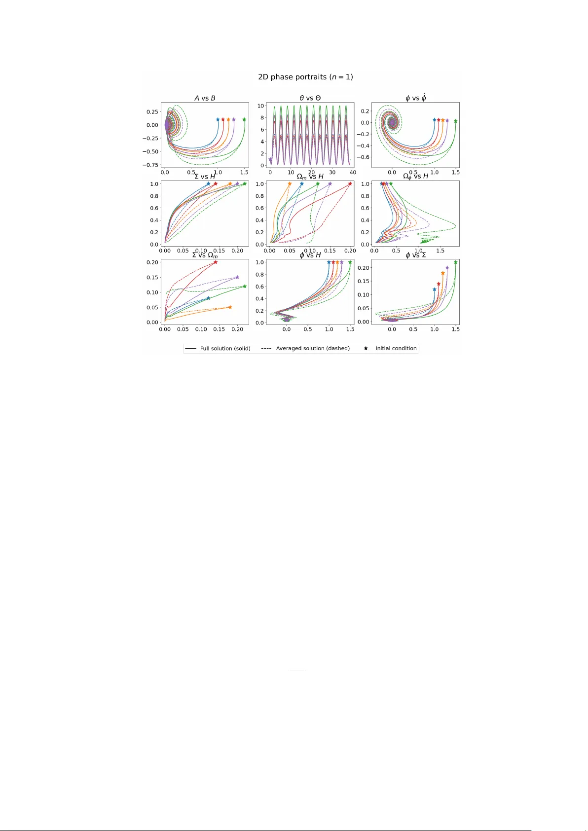
Dynamics of the Bianchi~V cosmological model inspired by quintessential $α$-attractors

Dynamics of the Bianc hi V cosmological mo del inspired b y quin tessen tial α -attractors Genly Leon 1,2,3 , ∗ Amare Abeb e 3,4 , † and Andronik os P aliathanasis 1,2,3,4 ‡ 1 Dep artamento de Matem´ atic as, Universidad Cat´ olic a del Norte, Avdeni da A ngamos 0610, Casil la 1280, Antofagasta, Chile, Antofagasta, Chile 2 Institute of Systems Scienc e, Durb an University of T e chnolo gy, Durb an 4000, South Afric a 3 Centr e for Sp ac e R ese ar ch, North-West University, Potchefstr o om 2520, South Afric a and 4 National Institute for The or etic al and Computational Scienc es (NITheCS), South Afric a. W e in vestigate scalar-field cosmologies in the Bianchi V spacetime using a dynamical- systems framew ork. Motiv ated b y represen tative α -attractor potentials - the E-model and T- mo del - we apply a veraging theorems and amplitude–phase reductions to monomial p otentials ∼ ϕ 2 n of the scalar field, which approximate the attractor mo dels near their minima, in the presence of matter with barotropic index γ . The reduced a veraged system admits fiv e generic isolated equilibria: Kasner v acua K ± 0 , the matter FLR W p oin t F , the scalar FLR W p oin t S , and the curv ature Milne-t yp e p oint K , together with sp ecial families for tuned ( n, γ ). W e find that K ± 0 are alw ays sources, F is generically a saddle but can act as a sink for γ < min { 2 n n +1 , 2 3 } , S is a sink if 0 < n < 1 2 and 2 n n +1 < γ ≤ 2, while K b ecomes a sink whenev er γ > 2 3 and n > 1 2 . These results demonstrate that isotropic FLR W α -attractor mo dels extend naturally to anisotropic Bianc hi V cosmologies: inflationary attractors remain robust, while the Milne-type curv ature solution emerges as the late-time state. I. INTR ODUCTION The standard cosmological mo del, commonly referred to as the Λ CDM mo del, assumes that the Universe is homogeneous and isotropic on sufficiently large, cosmological scales, according to the Cosmological Principle. Under these assumptions, the large-scale geometry of spacetime is describ ed by the F riedmann–Lema ˆ ıtre–Rob ertson–W alk er (FLR W) geometry [1]. The mo del also assumes the presence of dark comp onents. In particular, cold dark matter is in tro duced to address numerous gravitational phenomena, such as flat galaxy rotation curv es, the gro wth of large-scale structure, gravitational lensing, and the dynamics of galaxy clusters [2 – 8]. Moreov er, ∗ Electronic address: genly .leon@ucn.cl † Electronic address: amare.ab ebe@nithecs.ac.za ‡ Electronic address: anpaliat@phys.uoa.gr 2 the cosmological constant Λ [9] has b een introduced to describ e the dark energy comp onent of the Universe whic h driv es the late-time cosmic acceleration. The current accelerated phase of the univ erse is supp orted by v arious indep endent observ ational prob es, including T yp e Ia sup erno v ae, measuremen ts of the cosmic microw a ve background, and large-scale structure surveys [10 – 17]. Despite its minimal set of free parameters, the Λ CDM paradigm has prov en remark ably successful in providing a coheren t and precise description of current cosmological observ ations [12]. The Λ CDM mo del successfully describ es cosmic expansion, structure formation, and the statis- tical prop erties of the Univ erse using a minimal set of assumptions. Ho wev er, it still faces several serious theoretical and observ ational c hallenges. In particular, the fundamental microphysical na- ture of its dominan t comp onents, which accoun t for nearly 95% of the matter-energy con ten t of the Univ erse, remains unknown [18 – 21]. No dark matter particle has b een directly detected, and its existence is inferred only from gra vitational effects on galaxies, clusters, gravitational lensing, and large-scale structure, whereas dark energy is inferred from its role in driving the late-time accelerated expansion of the Univ erse [5, 6, 9]. In light of these challenges faced by the General Relativity (GR)–based Λ CDM framework, sev- eral complementary schools of though t hav e emerged in recent years. In general, these approac hes examine departures from one or more foundational assumptions of the concordance model. Some in vestigate mo difications to the gra vitational sector itself, by extending or altering Einstein’s field equations, while others relax the assumptions of large-scale homogeneity and isotropy , or consider more radical changes to the matter–energy con ten t of the univ erse [22 – 27]. In addition to mo difying the gra vitational sector or in tro ducing new dynamical degrees of free- dom, a complementary and physically well-motiv ated approach to addressing the limitations of the Λ CDM paradigm is to relax the assumption of exact isotropy at the level of the background spacetime. Within this broader con text, spatially homogeneous but anisotropic Bianchi-t yp e cos- mological mo dels provide a natural generalisation of the FLR W framew ork, enabling the systematic study of anisotropic expansion, shear dynamics, and their impact on cosmic ev olution [28, 29]. Suc h mo dels are particularly relev an t in light of observ ational anomalies at large angular scales and the question of whether the observed isotrop y of the universe is fundamental or an emergent late- time prop erty [30 – 34]. Among these, Bianc hi V spacetimes offer a controlled setting in which deviations from isotrop y can b e dynamically explored while main taining close contact with the standard cosmological mo del. This makes them esp ecially well suited to inv estigating mechanisms of isotropisation, the late-time suppression of anisotropies, and the role of matter fields—such as scalar fields—in driving the univ erse tow ards an effectively FLR W-like state. 3 In this context, n umerous studies hav e examined how mo difying the gravitational field can accoun t for phenomena traditionally attributed to dark comp onen ts, b y extending or altering Einstein’s field equations [35 – 37]. Within this broad class of mo dels, scalar fields play a central role and naturally arise in attempts to provide unified descriptions of b oth the early- and late-time ev olution of the universe [38 – 42]. Scalar fields are already a cornerstone of mo dern cosmology through the inflationary paradigm [43], and they also offer w ell-motiv ated dynamical alternativ es to a pure cosmological constan t at late times. These include quintessence models [44, 45], phantom fields [46], quin tom scenarios [47, 48], c hiral cosmologies [49, 50], and multi-scalar field frameworks capable of describing successiv e cosmological ep o c hs within a single theoretical setting [45, 51 – 53]. F rom a metho dological p ersp ectiv e, scalar-field cosmologies are particularly amenable to quali- tativ e analysis using to ols from dynamical systems theory [54 – 56], which enable systematic classifi- cation of cosmological solutions and rigorous assessmen t of their stabilit y prop erties. A well-kno wn example is chaotic inflation, in which the inflationary dynamics are driv en by a simple quadratic p oten tial [57, 58]. Complemen tary insight can b e gained from asymptotic metho ds and av erag- ing theory [59 – 62], which are esp ecially effective in probing the structure of the solution space of scalar-field cosmologies, b oth in v acuum and in the presence of additional matter comp onen ts [63 – 65]. Collectively , these approaches pro vide a flexible and mathematically robust framework for exploring extensions of the standard cosmological mo del while remaining closely connected to its phenomenological successes. One particularly imp ortan t application of scalar-field cosmology , one that has gained significant traction in recent y ears [60, 63 – 66], is the construction of a time-av eraged description of the under- lying cosmological dynamics, in which rapid scalar-field oscillations are systematically smo othed while the physically relev ant late-time b eha viour is preserved [60, 67 – 69]. This approach is par- ticularly well suited to mo dels go v erned by the Einstein–Klein–Gordon (EK G) system, in whic h the scalar field serv es as a dynamical source for the spacetime geometry [55, 56]. F rom b oth a ph ysical and observ ational p erspective, the fine-grained oscillatory dynamics of the scalar field are t ypically inaccessible, whereas their cum ulative, av eraged contribution to the energy–momentum tensor directly controls the large-scale expansion and effective matter conten t of the Universe. Av- eraging, therefore, provides a principled reduction of the full dynamical system, yielding effective cosmological equations that are simpler to analyse while remaining faithful to the underlying theory [70]. Within this framework, one can meaningfully address conceptual and phenomenological issues asso ciated with Λ CDM, including the emergence of effectiv e matter comp onents and dynamical alternativ es to a rigid cosmological constant. 4 A particular class of mo dels arises when the scalar field is endo wed with a nonlinear or p e- rio dic p oten tial, whic h naturally induces oscillatory b eha viour. Such dynamics o ccur in massive scalar-field mo dels, axion-like scenarios [71, 72], and in the p ost-inflationary evolution of the early Univ erse, and can p ersist ov er cosmological time scales [57, 59, 73, 74]. Although the field equa- tions are well-posed, the resulting dynamics are intrinsically multiscale [75, 76]: fast oscillations of the scalar field co exist with a slo wly evolving cosmological background. Since these microscopic oscillations do not directly affect cosmological observ ables, their av eraged effect gov erns the effec- tiv e energy densit y , pressure, and expansion rate. This clear separation of time scales provides a strong ph ysical motiv ation for using av eraging metho ds from dynamical systems theory , enabling the construction of effectiv e EK G systems that capture the slow cosmological ev olution without explicitly resolving the rapid oscillatory motion. In scalar-field cosmologies exhibiting oscillatory dynamics, regular oscillations ab out a sta- ble configuration typically arise only after initial transient phases—such as kinetic- or curv ature- dominated evolution—ha ve sufficien tly deca y ed. Once this regime is reac hed, the subsequen t ev o- lution is gov erned by the asymptotic structure of the underlying dynamical system, which fixes a veraged quan tities such as the effectiv e equation of state, the dilution rate of the scalar-field energy densit y , and the long-term b ehaviour of anisotropies or spatial curv ature. F rom a dynamical sys- tems p ersp ectiv e, this late-time b eha viour is commonly go v erned b y attractors, in v ariant manifolds, or scaling solutions that are largely insensitive to initial conditions. It is in this late-time regime that the av eraged description b ecomes more relev ant, as these asymptotic states determine the ef- fectiv e matter conten t, expansion laws, and stability prop erties of the cosmological m odel, thereb y pro viding a robust link b etw een microscopic scalar-field dynamics and macroscopic cosmological phenomenology [67, 77 – 82]. The pap er is organized as follows. In Section § I I we in tro duce the Bianc hi V geometry and deriv e the Einstein–Klein–Gordon equations in Hubble-normalized v ariables. In Section § I I I we dev elop the amplitude–phase reduction and av eraging analysis for monomial minima, and derive the reduced a veraged system. Numerical sim ulations and phase p ortraits are given in Section § IV. Finally , in Section § V we summarize our results and outline directions for future w ork. In App endix § A, w e provide a precise form ulation of the av eraging theorem for monomial scalar potentials, state the tec hnical h yp otheses, and pro ve the amplitude–phase and virial lemmas. F urthermore, we construct the near-iden tit y av eraging transformation with uniform remainder estimates, deduce the long-time closeness estimate and the coincidence of ω -limit sets, and classify the equilibrium p oints and relate them to the full system. 5 I I. BIANCHI V In this work, we will use the following parametrisation for the Bianc hi V metric spacetimes [83, Eq. (2.10)] and [84]: ds 2 = − dt 2 + a 2 ( t ) dx 2 + b 2 ( t ) e 2 x  dy 2 + a 4 ( t ) b 4 ( t ) dz 2  , (1) with the av erage Hubble and shear scalar parameters defined as H = ˙ a a , σ = ˙ a a − ˙ b b . (2) Although the line elemen t (1) dep ends on t wo scale factors, it should not b e confused with the lo cally rotationally symmetric (LRS) Bianc hi V spacetime ds 2 = − dt 2 + A 2 ( t ) dx 2 + B 2 ( t ) e 2 x  dy 2 + dz 2  . (3) The Bianc hi V spacetime b elongs to the Class B family of Bianchi mo dels, in which the gra vitational field equations are generically non-diagonal [85]. In our case, the non-diagonal constraint has already b een applied, fixing the third scale factor as a function of the remaining tw o [86], reducing the line element to its present form (1). Moreo ver, the tw o geometries are differen t; the LRS Bianc hi V supp orts matter sources with a non-v anishing flux term [87 – 89], whereas the geometry considered here do es not supp ort anisotropic solutions with a cosmic fluid with off-diagonal terms. Consequen tly , the spacetime (1) cannot b e reduced to LRS Bianc hi V geometry for any functional form of the scale factors. The t wo geometries coincide only in the op en FLR W spacetime. The evolution equations of the scalar field ϕ and matter energy densit y are: ¨ ϕ + 3 H ˙ ϕ + V ′ ( ϕ ) = 0 , (4a) ˙ ρ m + 3 γ H ρ m = 0 . (4b) Here, γ is the barotropic equation of state parameter relating the matter densit y to its pressure p m giv en by p m = ( γ − 1) ρ m . The rest of the equations are ˙ σ = − 3 H σ, (5a) ˙ a = aH, (5b) ˙ b = b ( H − σ ) , (5c) ˙ H = − 1 2  γ ρ m + 2 σ 2 + ˙ ϕ 2  − 1 a 2 , (5d) 6 and the constraint 3 H 2 = σ 2 + ρ m + 1 2 ˙ ϕ 2 + V ( ϕ ) + 3 a 2 . (5e) The choice of Bianc hi V spacetimes provides a new and non trivial context for the study of α –attractor potentials. Unlike the spatially flat FLR W mo dels, Bianchi V geometries incorp orate ne gative sp atial curvatur e together with anisotropic shear degrees of freedom. This combination allo ws one to prob e how inflationary and quintessen tial dynamics b eha v e in universes that are not exactly isotropic or spatially flat, thereby testing the robustness of attractor b eha vior under more general conditions and exploring the existence and b eha viour of anisotropic solutions, as well as the isotropic limit. A. The E–Model Poten tial W e start our analysis with the E –mo del p otential V ( ϕ ) = V 0  1 − e − q 2 3 α ϕ  2 n , (6) whic h is nonnegative and features a single global minimum at ( ϕ, V ) = (0 , 0), corresp onding to a Mink o wski v acuum solution ( H , ˙ ϕ, ϕ ) = (0 , 0 , 0). The p otential exhibits a plateau V → V 0 as ϕ → + ∞ , while for large negative field v alues it scales exponentially V ( ϕ ) ∼ V 0 e − 2 n q 2 3 α ϕ as ϕ → −∞ . (7) Near the origin, the p oten tial b ehav es as a p o wer law V ( ϕ ) ∼ ϕ 2 n as ϕ → 0 . (8) This asymmetric structure, with a steep exp onential tail and a flat inflationary plateau, mak es the E –model a prototypical example of α –attractor inflationary p otentials [90 – 93]. B. The T–Model Poten tial W e now consider the T–mo del p oten tial [90, 92] V ( ϕ ) = V 0 tanh 2 n  ϕ √ 6 α  , (9) a nonnegative function symmetric under ϕ 7→ − ϕ , due to the o dd parity of the hyperb olic tangen t and the even exponent 2 n . The p otential attains its global minimum at ϕ = 0, where V (0) = 0, and thus admits a Mink owski v acuum solution at ( H , ˙ ϕ, ϕ ) = (0 , 0 , 0). 7 As ϕ → ±∞ , the h yp erb olic tangen t saturates to ± 1, and the p oten tial asymptotes to a finite plateau V ( ϕ ) → V 0 . This yields t wo symmetric asymptotic de Sitter states, in contrast to the E –model, which features a single plateau as ϕ → + ∞ and an exp onential deca y as ϕ → −∞ . The double–plateau structure of the T–p oten tial is particularly relev ant in cosmological scenar- ios inv olving b ouncing, cyclic, or emergent dynamics, where the scalar field may tra verse b oth asymptotic regimes. Near the origin, the T–p oten tial b ehav es as V ( ϕ ) ∼ V 0  ϕ √ 6 α  2 n as ϕ → 0 , (10) matc hing the small–field b ehavior of the E –mo del. This ensures that b oth p otentials supp ort similar early–time dynamics near the Minko wski p oint, while differing in their global structure and asymptotic b eha vior. In summary , the T–p otential provides a symmetric, b ounded deformation of the standard p o w er–law p oten tial, with a cen tral Mink owski minim um and a double de Sitter plateau. Its compact analytic form makes it w ell-suited to dynamical systems analysis, particularly when com- bined with angular compactification techniques that render the state space regular and enable a global classification of asymptotic regimes. A complementary line of research is due to Alho and Mena [94], who developed a global dy- namical systems formulation for flat Rob ertson–W alk er cosmologies with Y ang–Mills fields and a p erfect fluid. Their framework established rigorous results on the global dynamics, including asymptotic source dominance in b oth time directions. F or the pure m assless Y ang–Mills case, they em b edded explicit solutions into a compact state–space picture, clarifying their global role. This w ork illustrates the strength of compact dynamical systems metho ds in extending lo cal analyses to global classifications, and provides a metho dological precedent for the compactification and a veraging techniques employ ed here. An imp ortant related contribution is Alho et al. [95], which studied minimally coupled scalar fields with monomial p oten tials V ( ϕ ) = ( λϕ ) 2 n / (2 n ) interacting with a p erfect fluid in flat Rob ertson–W alk er spacetimes. Introducing a friction–lik e term Γ( ϕ ) = µϕ 2 p , they identified a bifurcation at p = n/ 2: for p < n/ 2 the future dynamics admit a v ariety of attractors, while for p > n/ 2 the asymptotics resemble the non–interacting case. Sp ecial cases yield Li´ enard–t yp e dy- namics or new attractors driving late–time acceleration, while p = n/ 2 pro duces fluid–dominated or oscillatory b ehaviour. Crucially , they show ed that a quasi–de Sitter inflationary solution alwa ys exists tow ard the past, suggesting new realizations of quintessen tial inflation. 8 Finally , Alho and Uggla [96] extended the compact dynamical systems framew ork to quin tessen- tial α –attractor inflation, unifying early–time inflation with late–time quin tessence. In this form u- lation, the inflationary attractor corresp onds to the unstable cen ter manifold of a de Sitter fixed p oin t, while compactification ensures that Mink owski v acua, de Sitter plateaus, and exp onen tial tails are consistently incorporated. Their results demonstrate that the E – and T –p oten tials em b ed naturally into the quin tessen tial α –attractor paradigm. Based on the ab o v e discussion, we proceed with the av eraging strategy in the following sections. I I I. A VERA GING NEAR THE MINIMUM OF THE POTENTIALS Rescaling V 0 , the E – and T –p oten tials reduce near ϕ = 0 to the monomial scalar field p oten tial V ( ϕ ) = µ 2 n 2 n ϕ 2 n , n > 0 . (11) The corresp onding Klein–Gordon equation in the Bianchi V spacetime is ¨ ϕ + 3 H ˙ ϕ + µ 2 n ϕ 2 n − 1 = 0 . (12) The matter conserv ation la w, anisotrop y ev olution, and scale-factor dynamics follow from Eqs. (4b)–(5c) and the constrain t is (5e). A. Amplitude–phase represen tation Near the minimum of the monomial p otential, the field oscillates rapidly . T o capture this dynamics, we introduce ϕ ( t ) = A ( t ) cos θ ( t ) , (13) with slowly v arying amplitude A ( t ) and rapidly v arying phase θ ( t ). Differentiating gives ˙ ϕ = − A ˙ θ sin θ + ˙ A cos θ , (14) ¨ ϕ = − A ( ˙ θ ) 2 cos θ − A ¨ θ sin θ − 2 ˙ A ˙ θ sin θ + ¨ A cos θ . (15) Substituting into (12) yields ¨ A cos θ − A ( ˙ θ ) 2 cos θ − A ¨ θ sin θ − 2 ˙ A ˙ θ sin θ + 3 H ( ˙ A cos θ − A ˙ θ sin θ ) + µ 2 n A 2 n − 1 cos 2 n − 1 θ = 0 . (16) 9 In tro duce auxiliary v ariables B ≡ ˙ A, Θ ≡ ˙ θ , ˙ B = ¨ A, ˙ Θ = ¨ θ . (17) Equation (16) b ecomes ( ˙ B − A Θ 2 + 3 H B + µ 2 n A 2 n − 1 cos 2 n − 2 θ ) cos θ + ( − A ˙ Θ − 2 B Θ − 3 H A Θ) sin θ = 0 . (18) Since cos θ and sin θ are linearly indep enden t, the co efficients must v anish separately: ˙ B = A Θ 2 − 3 H B − µ 2 n A 2 n − 1 cos 2 n − 2 θ , ˙ Θ = − 2 B Θ A − 3 H Θ , (19) together with ˙ A = B and ˙ θ = Θ. B. Exact amplitude–phase system Coupling to gravit y yields the full first-order system ˙ A = B , (20a) ˙ B = A Θ 2 − 3 H B − µ 2 n A 2 n − 1 cos 2 n − 2 θ , (20b) ˙ θ = Θ , (20c) ˙ Θ = − 2 B Θ A − 3 H Θ , (20d) ˙ Σ = − (2 − q ) Σ H , (20e) ˙ Ω m = Ω m (2 q − 3 γ + 2) H , (20f ) ˙ H = − (1 + q ) H 2 , (20g) with deceleration parameter q = 2Σ 2 + 1 2 (3 γ − 2)Ω m + 1 3 H 2   − A Θ sin θ + B cos θ  2 − µ 2 n 2 n ( A cos θ ) 2 n  . (21) The normalized scalar fraction, expressed in terms of the amplitude–phase v ariables, is Ω ϕ ( A, B , θ , Θ) = 1 3 H 2  1 2  − A Θ sin θ + B cos θ  2 + µ 2 n 2 n ( A cos θ ) 2 n  . (22) The only division b y A o ccurs in ˙ Θ. Since A is the oscillation amplitude, it can b e chosen nonnegativ e and does not generically cross zero for contin uous oscillatory solutions. If A b ecomes v ery small in numerical runs, one ma y switc h to energy–angle v ariables or absorb the sign of A in to θ to enforce A ≥ 0. Th us, the amplitude–phase system remains regular across ϕ = 0 and av oids the ϕ − 1 singularit y . 10 Av eraging is a coarse-graining pro cedure in which rapidly oscillating quantities are replaced b y their mean v alues ov er one p erio d of the fast v ariable. This yields an effective dynamical system for the slo wly v arying amplitudes and phases. In the fast–oscillation regime, av eraging extracts the secular evolution while filtering out cycle–to–cycle fluctuations, providing a simplified yet accurate description of the long-term dynamics. C. Av eraged amplitude–phase ev olution Av eraging the oscillatory terms in (20) o v er one fast cycle of θ yields cos 2 n θ = (2 n )! 2 2 n ( n !) 2 , cos 2 n − 2 θ = (2 n − 2)! 2 2 n − 2 [( n − 1)!] 2 . (23) The av eraged amplitude–phase system is then ˙ A = B , (24a) ˙ B = A Θ 2 − 3 H B − µ 2 n A 2 n − 1 (2 n − 2)! 2 2 n − 2  ( n − 1)!  2 , (24b) ˙ θ = Θ , (24c) ˙ Θ = − 2 B Θ A − 3 H Θ , (24d) ˙ Σ = − (2 − q ) Σ H , (24e) ˙ Ω m = Ω m (2 q − 3 γ + 2) H , (24f ) ˙ H = − (1 + q ) H 2 , (24g) with the av eraged deceleration parameter q = 2Σ 2 + 1 2 (3 γ − 2) Ω m + 1 2 (1 + 3 w ϕ ) Ω ϕ , (25) where Ω ϕ denotes the effective scalar contribution. Av eraging (22) ov er one cycle gives ⟨ sin 2 θ ⟩ = ⟨ cos 2 θ ⟩ = 1 2 , ⟨ sin θ cos θ ⟩ = 0 , (26) so the av eraged scalar fraction b ecomes Ω ϕ = 1 3 H 2  1 4  A 2 Θ 2 + B 2  + µ 2 n 2 n A 2 n (2 n )! 2 2 n ( n !) 2  . (27) 11 D. Av eraging pro cedure for rapid oscillations When ω ( A ) ≫ H , the scalar field oscillates muc h faster than the Hubble expansion, so one can a verage ov er a p erio d of θ . 1. F r e quency F rom (16), the leading balance is − A ( ˙ θ ) 2 cos θ ∼ µ 2 n A 2 n − 1 cos 2 n − 1 θ . (28) Dividing by A cos θ gives ( ˙ θ ) 2 ≈ µ 2 n A 2 n − 2 cos 2 n − 2 θ . (29) Av eraging cos 2 n − 2 θ yields ( ˙ θ ) 2 · 1 2 = µ 2 n A 2 n − 2 (2 n )! 2 2 n ( n !) 2 , (30) so the effective frequency is ˙ θ = ω ( A ) := µ n A n − 1  (2 n )! 2 2 n − 1 ( n !) 2  1 / 2 . (31) 2. Amplitude evolution The friction term 3 H ˙ ϕ = 3 H ( − A ˙ θ sin θ + ˙ A cos θ ) (32) a verages to a secular drift in A ( t ). Comparing ρ ϕ ∝ A 2 n with the av eraged loss − 3 H ˙ ϕ 2 = − 3 n n +1 H ρ ϕ , (33) giv es ˙ A = − 3 H n +1 A. (34) 3. Aver age d dynamics Equations (31) and (34) define the av eraged system, v alid when ω ( A ) ≫ H . 12 4. Sc aling laws and effe ctive fluid In tegration of (34) giv es A ( t ) ∝ a − 3 n +1 , ρ ϕ ∝ a − 6 n n +1 . (35) The virial relation ˙ ϕ 2 = n V ( ϕ ) implies p ϕ = n − 1 n +1 ρ ϕ , w ϕ = n − 1 n +1 , γ ϕ = 2 n n +1 . (36) Th us, the scalar b eha v es as a fluid with barotropic index γ ϕ and dilution law from (35). 5. Exact vs. aver age d evolution The exact law is Ω ′ ϕ = − 6 x 2 + 2( q + 1) Ω ϕ , (37) with Ω ϕ := x 2 + y 2 , x := ˙ ϕ √ 6 H , y := µ n ϕ n √ 6 n H , (38) and q = 2Σ 2 + 1 2 (3 γ − 2) Ω m + 2 x 2 − y 2 . (39) In the rapid oscillation regime, the virial relation gives x 2 = n n +1 Ω ϕ , (40) so (37) av erages to Ω ′ ϕ = Ω ϕ  2 q − 3 2 n n + 1 + 2  , (41) with constraint Σ 2 + Ω m + Ω k + Ω ϕ = 1 . (42) E. Remarks Amplitude–phase or action–angle v ariables [84, 97, 98] remov e the ϕ − 1 singularit y and ensure regularit y across oscillations while preserving numerical stabilit y . 13 F. Connection to the av eraged system Av eraging (20) ov er one fast oscillation p eriod repro duces the slow amplitude law (34), con- sisten t with the fluid description (36). Hence, the exact amplitude–phase system is asymp- totically consistent with the a veraged dynamics and reco v ers the late-time barotropic index w ϕ = ( n − 1) / ( n + 1) for the p oten tial index n > 0. The resulting system is Σ ′ =  2(Σ 2 − 1) + 1 2 (3 γ − 2) Ω m + (2 n − 1) ( n + 1) Ω ϕ  Σ , (43a) Ω ′ m =  4Σ 2 + (3 γ − 2)  Ω m − 1  + 2(2 n − 1) ( n + 1) Ω ϕ  Ω m , (43b) Ω ′ ϕ =  4Σ 2 + (3 γ − 2) Ω m + 2(2 n − 1) ( n + 1) (Ω ϕ − 1)  Ω ϕ . (43c) with phase space defined b y the compact constraint Σ 2 + Ω m + Ω ϕ ≤ 1 . (44) Equilibrium states are obtained. W e hav e isolated p oints (generic n, γ ): (Σ , Ω m , Ω ϕ ) = ( − 1 , 0 , 0) Kasner v acuum K − 0 , (Σ , Ω m , Ω ϕ ) = (0 , 0 , 1) Scalar FLR W S , (Σ , Ω m , Ω ϕ ) = (0 , 1 , 0) Matter FLR W F , (Σ , Ω m , Ω ϕ ) = (1 , 0 , 0) Kasner v acuum K + 0 , (Σ , Ω m , Ω ϕ ) = (0 , 0 , 0) Curv ature p oint K . F or certain ( n, γ ), the system admits one-dimensional families: • n = 1 2 , γ = 2 3 : line Σ = 0 with arbitrary (Ω m , Ω ϕ ) sub ject to (44). • n = 1 2 : curve Σ = 0, Ω m = 0, arbitrary Ω ϕ . • γ = 2 3 : curve Σ = 0, Ω ϕ = 0, arbitrary Ω m . • γ = 2 n 1+ n : mixed scalar–matter scaling line Σ = 0, Ω ϕ = 1 − Ω m , interpolating b etw een F and S . • γ = 2: curve Ω m = 1 − Σ 2 , Ω ϕ = 0, a family of matter–curv ature states. The reduced av eraged system exhibits b oth isolated equilibria and contin uous families of solu- tions that interpolate b et ween the Kasner v acua, the matter FLR W p oint, the scalar FLR W p oin t, 14 and the curv ature p oin t. As summarized in T able I, these five generic equilibria— K ± 0 , F , S , and K —p ossess eigenv alue sp ectra and stabilit y prop erties that dep end sensitively on the parameters ( n, γ ), giving rise to sources, saddles, and sinks in differen t regimes. The stabilit y conditions in T able I further demonstrate the co existence of multiple attractors, with b oth S and K capable of acting as sinks dep ending on ( n, γ ), thereb y shaping the global phase flow of the system. T able I: Equilibria and eigenv alues of the av eraged system (43) for general n > 0 and 0 ≤ γ ≤ 2. Equilibrium Eigen v alues Stabilit y K ± 0 at ( ± 1 , 0 , 0) n 6 1+ n , 4 , 6 − 3 γ o Source for 0 ≤ γ < 2; nonh yp erb olic at γ = 2 F at (0 , 1 , 0) n 3 2 ( γ − 2) , − 2 + 3 γ , − 6 n 1+ n + 3 γ o Sink if γ < min { 2 n n +1 , 2 3 } ; nonhyperb olic at γ = 2 3 , 2 n n +1 , or 2; saddle otherwise S at (0 , 0 , 1) n − 3 1+ n , 4 − 6 1+ n , 6 n 1+ n − 3 γ o Sink if 0 < n < 1 2 , 2 n n +1 < γ ≤ 2; nonh yp erb olic at n = 1 2 or n = γ 2 − γ ; saddle otherwise K at (0 , 0 , 0) n − 2 , − 4 + 6 1+ n , 2 − 3 γ o Sink if γ > 2 3 and n > 1 2 ; nonhyperb olic at n = 1 2 or γ = 2 3 ; saddle otherwise IV. NUMERICAL IMPLEMENT A TION In practice, w e in tegrate b oth the full amplitude–phase system (20) and the a veraged reduced system (36) in cosmic time t . The state vector is defined as ( A, B , θ , Θ , Σ , Ω m , H ), with ϕ and ˙ ϕ reconstructed via (13), and (14). The av eraged system evolv es (Ω ϕ , Ω m , Σ , H ), thereby smo othing o ver the fast oscillations. Both systems are solv ed using a stiff in tegrator ( Radau ) with tight tolerances o ver the interv al t ∈ [0 , T max ], with T max = 40 , 200. Short integration times highlight the rapid oscillations, and long times rev eal the capture of the transitionary dynamics, the late– time b eha vior. At each step, Ω ϕ is computed from (22) and used to initialize the av eraged system, ensuring consistent initial conditions. The resulting tra jectories are then compared in the three– dimensional phase space (Ω ϕ , Σ , Ω m ) and its t w o–dimensional pro jections. These initial conditions explore differen t balances among scalar-field energy , shear, and matter fractions. By computing Ω ϕ from (22) at t = 0 and feeding it in to the av eraged system, b oth descriptions start consistently , allowing a direct comparison of how the av eraged dynamics track the full oscillatory b eha viour. 15 T able I I: Initial conditions for the full amplitude–phase system with n = 2 , 3. The colored stars sho w the reference colors used in the plots. Set A (0) B (0) θ (0) Θ(0) Σ(0) Ω m (0) H (0) ⋆ 1 1.0 0.1 0.05 1.0 0.12 0.08 1.0 ⋆ 2 1.2 0.1 0.05 1.0 0.18 0.05 1.0 ⋆ 3 1.5 0.1 0.05 1.0 0.22 0.12 1.0 ⋆ 4 1.1 0.1 0.05 1.0 0.14 0.20 1.0 ⋆ 5 1.3 0.1 0.05 1.0 0.20 0.15 1.0 A. Dynamics in the co ordinates ( A, B , θ , Θ , Σ , Ω m , H ) Figures 1 and 2 illustrate the accuracy of the av eraged amplitude–phase system in repro ducing the slow dynamics of the full mo del. F or n = 1 and n = 2, the av eraged tra jectories capture the en velope of the oscillations in A ( t ), B ( t ), and Θ( t ), while eliminating the fast phase dep endence on θ . The shear Σ( t ) and matter densit y parameter Ω m ( t ) show close agreement b etw een the tw o descriptions, confirming that the a veraged system preserves the essential gra vitational bac kreaction. Most imp ortantly , the scalar con tribution Ω ϕ ( t ) is well track ed b y the av eraged system, v alidating the effective fluid description with barotropic index w ϕ = ( n − 1) / ( n + 1). Figures 3 and 4 presen t the corresponding 2D phase–space p ortraits. The pro jections (including A vs. B , θ vs. Θ, B vs. θ , B vs. Θ, ϕ vs. ˙ ϕ , Σ vs. H , Ω m vs. H , Ω ϕ vs. H , Σ vs. Ω m , ϕ vs. H , and ϕ vs. Σ) demonstrate that the av eraged s ystem repro duces the slo w manifold structure of the full dynamics. The av eraged tra jectories smo oth out the fast oscillations in θ , while the full system shows the underlying oscillatory modulation. Both descriptions con verge tow ard the same attractor manifold. Figures 5 and 6, show the 3D phase p ortraits. The plots in ( ϕ, ˙ ϕ, H ) and ( ϕ, ˙ ϕ, A ) indicate how the scalar field dynamics couple to the Hubble parameter and amplitude, while the p ortraits in (Ω m , H, Σ) and (Ω ϕ , H, Σ) to show the relation b et w een matter, scalar energy , and shear. Small deviations are observed in the early-time oscillatory regime, but they diminish as the system ev olves, which means that the av eraged equations provide a reliable autonomous approximation to the long-term dynamics. The absence of closed p erio dic structures in the 2D and 3D p ortraits is a direct consequence of the cosmological dynamics. F or n = 1, the full system exhibits spirals in the ( ϕ, ˙ ϕ ) plane, reflecting damp ed oscillations of the scalar field. These spirals collapse inw ard due to Hubble friction, whic h 16 Figure 1: Time ev olution of the dynamical v ariables for n = 1. Solid lines correspond to the a veraged system, while dashed lines corresp ond to the full system. Initial conditions are tak en from T able I I. con tinuously drains energy from the field and preven ts the tra jectories from forming closed lo ops. The system is non-autonomous since H ( t ) itself evolv es, breaking time-translation inv ariance and eliminating the possibility of exact perio dic orbits. By construction, the a veraged amplitude–phase system smo oths out the fast oscillations in θ , so its tra jectories cannot displa y p eriodicity either. As illustrated in the 2D and 3D p ortraits, b oth the full and a v eraged systems exhibit slow drifts to ward attractors rather than repeating cycles, confirming that the absence of p erio dic structures is a physical feature of cosmological damping rather than a n umerical artifact. B. Dynamics of the av eraged system in the co ordinates (Σ , Ω m , Ω ϕ ) T o explore the v alidit y of the av eraging pro cedure, we compare tra jectories of three dynamical systems: the full amplitude–phase equations, the av eraged amplitude–phase system, and the re- 17 Figure 2: Time ev olution of the dynamical v ariables for n = 2. Solid lines correspond to the a veraged system, while dashed lines corresp ond to the full system. Initial conditions are tak en from T able I I. duced av eraged system in the compact co ordinates (Σ , Ω m , Ω ϕ ). The initial conditions are c hosen from representativ e sets (see T able I I), and each set is plotted with a distinct color. Solid lines denote the full system, dashed lines the av eraged system, and dashed–dotted lines the reduced av- eraged system. Stars mark initial conditions tak en from T able II. This visual comparison highlights ho w the av eraged and reduced systems capture the coarse-grained dynamics of the full tra jectories, filtering out fast oscillations while preserving the long-term flow tow ard attractors. F or n = 1 and n = 2 with γ = 1, the Kasner p oints are unstable sources, the matter and scalar FLR W p oin ts are saddles, and the curv ature p oin t K is the global attractor. The plots confirm this classification: tra jectories originate near anisotropic or mixed states, pass close to matter or scalar saddles, and even tually con verge to the curv ature sink. The agreement b etw een the three systems demonstrates that the a v eraging pro cedure faithfully repro duces the qualitative dynamics 18 Figure 3: 2D phase–space p ortraits for n = 1. Pro jections include A vs. B , θ vs. Θ, B vs. θ , B vs. Θ, ϕ vs. ˙ ϕ , and ϕ vs. H . The av eraged system repro duces the slow manifold structure of the full dynamics. Initial conditions are taken from T able I I. of the full equations. V. CONCLUSIONS W e studied Bianchi V cosmologies within a compact dynamical systems framew ork. Motiv ated b y the α -attractor models in FLR W [96], the late-time dynamics w ere studied through monomial p oten tials V ( ϕ ) ∼ ϕ 2 n , which approximate the attractor mo dels near their minima. Tw o complemen tary a veraging pro cedures w ere dev elop ed. Amplitude–phase a veraging replaces rapidly oscillating trigonometric terms in the exact s ystem by their cycle a verages, yielding a regularized system that preserves equilibrium classification and clarifies the role of scalar oscillations as effective fluids. Coarse–grained a veraging, v alid when ω ( A ) ≫ H , deriv es explicit secular la ws for amplitude and frequency , showing that ˙ A = − 3 H n +1 A and ω ( A ) ∝ A n − 1 . This connects microscopic oscillations to macroscopic dilution la ws, yielding a reduced av eraged system. The a v eraging theorem established in Appendix A provides the mathematical foundation for 19 Figure 4: 2D phase–space p ortraits for n = 2. Pro jections include A vs. B , θ vs. Θ, B vs. θ , B vs. Θ, ϕ vs. ˙ ϕ , and ϕ vs. H . The av eraged system repro duces the slow manifold structure of the full dynamics. Initial conditions are taken from T able I I. the analytic reductions used in this w ork. Under assumptions (H1)–(H4), solutions of the full Einstein–Klein–Gordon system and of the av eraged system remain O ( ε )-close for times of order 1 /ε , ensuring that the av eraged system faithfully repro duces the global attractor structure of the full dynamics. In particular, the scalar sector b eha ves as an effectiv e barotropic fluid with index γ ϕ = 2 n n +1 , up to O ( ε ) corrections, and ω -limit sets coincide b et ween the full and av eraged flows. Th us, near the p otential minimum, the oscillatory regime is consisten tly describ ed b y an effective fluid with w ϕ = n − 1 n +1 and dilution la w ρ ϕ ∝ a − 6 n/ ( n +1) , bridging microscopic scalar oscillations with macroscopic cosmological dynamics. The matter solution acts as an attractor only when the scalar sector dilutes faster than matter, i.e. 6 n n + 1 > 3 γ , (45) so that ρ ϕ deca ys more rapidly than ρ m ∝ a − 3 γ . F or γ = 1, this condition holds for n > 1, while for n = 1 the scalar b eha v es as dust and curv ature even tually dominates. The qualitativ e b ehaviour 20 Figure 5: 3D phase–space p ortraits for n = 1. T ra jectories in ( ϕ, ˙ ϕ, H ) and ( ϕ, ˙ ϕ, A ) confirm that the av eraged system pro vides a reliable autonomous approximation to the long-term dynamics. Initial conditions are tak en from T able I I. of the scalar sector and the corresp onding attractor structure are summarized in T able I I I. The reduced a veraged system admits five generic isolated equilibria: Kasner v acua K ± 0 , the matter FLR W p oin t F , the scalar FLR W p oint S , and the curv ature Milne-type p oint K , together with sp ecial families for tuned ( n, γ ). W e find that K ± 0 are alw ays sources, F is generically a saddle but can act as a sink for γ < min { 2 n n +1 , 2 3 } , S is a sink if 0 < n < 1 2 and 2 n n +1 < γ ≤ 2, while K b ecomes a sink whenev er γ > 2 3 and n > 1 2 . These results demonstrate that isotropic FLR W α -attractor models extend naturally to anisotropic Bianc hi V cosmologies: inflationary attractors remain robust, while the Milne-t yp e curv ature solution emerges as the late-time state. 21 Figure 6: 3D phase–space p ortraits for n = 2. T ra jectories in ( ϕ, ˙ ϕ, H ) and ( ϕ, ˙ ϕ, A ) confirm that the av eraged system pro vides a reliable autonomous approximation to the long-term dynamics. Initial conditions are tak en from T able I I. In conclusion, amplitude–phase av eraging provides a detailed analytic reduction of the oscil- latory dynamics, while coarse–grained a veraging yields explicit secular la ws for amplitude and frequency . Their syn thesis establishes a robust and efficient framework: the reduced av eraged sys- tem captures the essential late–time b ehaviour of homogeneous Bianchi V cosmologies, regularizes b oundaries, and clarifies in v ariant sets, while greatly impro ving computational efficiency . This uni- fied approac h demonstrates that the attractor structure familiar from FLR W α –attractor mo dels p ersists in anisotropic settings, ensuring that the late–time dynamics conv erge to the curv ature sink K after transien t matter or scalar phases. F uture w ork will extend this analysis to the full 22 Figure 7: T ra jectories in (Ω ϕ , Σ , Ω m ) for n = 1, γ = 1. Solid lines: full system; dashed lines: a veraged system; dash–dotted lines: reduced av eraged system. Stars mark initial conditions taken from T able I I. n Effective equation of state w ϕ Dilution law ρ ϕ Late-time attractor 1 0 (dust-like) a − 3 Curv ature sink K after matter saddle 2 1 3 (radiation-lik e) a − 4 Curv ature sink K after radiation saddle T able I I I: Summary of effectiv e scalar b ehaviour and attractor structure for monomial p oten tials V ( ϕ ) ∼ ϕ 2 n with γ = 1. ev aluation of the E and T p oten tials, thereby connecting the lo cal monomial appro ximation with the global attractor structure of α –attractor cosmologies. 23 Figure 8: T ra jectories in (Ω ϕ , Σ , Ω m ) for n = 2, γ = 1. Solid lines: full system; dashed lines: a veraged system; dash–dotted lines: reduced av eraged system. Stars mark initial conditions taken from T able I I. Ac kno wledgments F unded by Agencia Nacional de In vestigaci´ on y Desarrollo (ANID), Chile, through Proy ecto F ondecyt Regular 2024, F olio 1240514, Etapa 2025. A.A. gratefully ac knowledges the hospitality of Prof. Genly Leon and his researc h group at the Univ ersidad Cat´ olica del Norte (UCN), An tofa- gasta, during his visit, where this w ork w as initiated and largely carried out. W e also extend our gratitude to the Vicerrector ´ ıa de Inv estigaci´ on y Desarrollo T ecnol´ ogico (VRIDT) of UCN for the scien tific supp ort provided through the N ´ ucleo de Inv estigaci´ on en Geometr ´ ıa Diferencial y Aplica- ciones, according to Resolution VRIDT No. 096/2022, and through the N ´ ucleo de Inv estigaci´ on en Simetr ´ ıas y la Estructura del Universo (NISEU), according to Resolution VRIDT No. 200/2025. 24 App endix A: Averaging: rigorous statement and pro of 1. Notation and functional setting Let X ( t ) ∈ R m denote the vector of slow Hubble-normalized v ariables used in the main text (for example, Ω ϕ , Σ , Ω m , . . . ). Let K ⊂ R m b e the compact forward-in v ariant set obtained by the compactification describ ed in Sections I I–I I I. Fix a norm ∥ · ∥ on R m (equiv alen t to the Euclidean norm). F or r ∈ N denote by C r ( K ) the Banac h space of r -times contin uously differen tiable vector fields on K with the usual C r -norm. 2. Assumptions • (H1) Regularity and compactness. The full EK G v ector field in the compact Hubble-normalized v ariables is C r on an op en neigh b ourho o d of a compact forw ard-inv ariant set K ⊂ R m , with r ≥ 3. All deriv ativ es up to order r are uniformly bounded there; denote b y M r > 0 a uniform b ound for the C r -norm. • (H2) P erio dic family and mo dulation. There exists an amplitude in terv al I = [ A min , A max ] with 0 < A min < A max < ∞ such that for eac h A ∈ I a C r − 1 family of 2 π -p erio dic profiles Φ( θ ; A ) solv es the frozen oscillator at amplitude A . The fast phase and amplitude satisfy ˙ θ = ω ( A ) + ρ ( A, X , t ) , ω ( A ) = µ n A n − 1  (2 n )! 2 2 n − 1 ( n !) 2  1 / 2 , (A1) with the explicit b ound | ρ ( A, X , t ) | ≤ C ρ H ( t ), and ˙ A = − 3 H n + 1 A + δ A ( A, X , t ) , (A2) with | δ A ( A, X , t ) | ≤ C A H ( t ) 2 ω ( A ) . The constants C ρ , C A > 0 dep end only on M r and I . • (H3) Scale separation. Define ε := sup X ∈K A ∈ I H ω ( A ) . (A3) There exists ε 0 > 0 such that 0 < ε ≤ ε 0 ≪ 1. In particular inf A ∈ I ω ( A ) > 0. • (H4) Homological solv ability . F or all Y ∈ K and A ∈ I the op erator ω ( A ) ∂ θ is inv ert- ible on zero-mean 2 π -p erio dic functions and the small-divisor denominators arising in the a veraging construction are uniformly bounded b elo w by a p ositive constan t prop ortional to inf A ∈ I ω ( A ). 25 3. Auxiliary results Lemma A.1 (P erio dic family) . Under (H1) and for the monomial p otential, ther e exists an ampli- tude interval I and a C r − 1 family of 2 π -p erio dic pr ofiles Φ( θ ; A ) solving the fr ozen oscil lator at fixe d amplitude A . The fr e quency ω ( A ) = µ n A n − 1  (2 n )! 2 2 n − 1 ( n !) 2  1 / 2 is C r − 1 on I and inf A ∈ I ω ( A ) > 0 . Pr o of. The frozen scalar equation at fixed energy (or amplitude) defines a nonlinear oscillator with a nondegenerate minimum. Standard existence and smooth dep endence results for p erio dic orbits (implicit function theorem applied to the Poincar ´ e map or Lyapuno v–Schmidt reduction) yield the family Φ( θ ; A ) and smo othness in A . The stated low er b ound on ω ( A ) follo ws b y choosing I a w ay from zero amplitude. Lemma A. 2 (Amplitude–phase mo dulation) . Under (H1)–(H3), ther e exist c onstants C ρ , C A > 0 and T > 0 such that every solution with initial data in a neighb ourho o d of K admits ϕ ( t ) = A ( t ) Φ  θ ( t ); A ( t )  , (A4) with ˙ θ = ω ( A ) + ρ ( A, X , t ) , ˙ A = − 3 H n + 1 A + δ A ( A, X , t ) , (A5) and the uniform b ounds | ρ ( A, X , t ) | ≤ C ρ H ( t ) , | δ A ( A, X , t ) | ≤ C A H ( t ) 2 ω ( A ) (A6) for al l t ∈ [0 , T ] , X ∈ K , and A ∈ I . Pr o of. Pro ject the full scalar equation on to the tangent and normal directions of the p erio dic family Φ( θ ; A ) using a phase normalization condition. The coupling terms are prop ortional to H and its deriv ativ es; uniform C r -b ounds and compactness of K pro duce the stated constants and inequalities. This is the standard deriv ation of mo dulation in av eraging theory . Lemma A.3 (Virial relation with explicit error) . Under (H1)–(H3), for the normalize d kinetic variable x and p otential c ontribution y asso ciate d to ϕ , 1 2 π Z 2 π 0 x 2 ( θ ) dθ = n n + 1 1 2 π Z 2 π 0  x 2 + y 2  dθ + E 1 , (A7) with |E 1 | ≤ C 1 ε, (A8) for some C 1 > 0 dep ending only on M r and I . 26 Pr o of. F or the frozen p erio dic orbit, the exact virial ratio ⟨ x 2 ⟩ : ⟨ y 2 ⟩ = n : 1 holds. F or the slo wly mo dulated orbit, the difference b etw een the time av erage and the frozen av erage is controlled by the mo dulation remainders from Lemma A.2; integrating yields the stated O ( ε ) b ound. Prop osition A.4 (Near-identit y transform and remainder) . Under (H1)–(H4) ther e exists a ne ar-identity C r − 2 change of variables X = Y + ε U ( Y , θ , ε ) , (A9) with U 2 π -p erio dic in θ and uniformly b ounde d on K × S 1 , such that the tr ansforme d system for Y r e ads ˙ Y = F 0 ( Y ) + R ( Y , θ , ε ) , (A10) wher e F 0 is the aver age d ve ctor field and sup Y ∈K , θ ∈ S 1 ∥R ( Y , θ , ε ) ∥ ≤ C 2 ε 2 . (A11) The c orr e ction U solves the homolo gic al e quation ω ( Y ) ∂ θ U ( Y , θ ) = e G ( Y , θ ) , (A12) with e G the zer o-me an oscil latory p art of the original ve ctor field; solvability fol lows fr om (H4). Pr o of. W rite the system on the slow time τ = εt , decomp ose the righ t-hand side into a v eraged and oscillatory parts, and solve the homological equation for the p eriodic correction U . Inv ertibility of ω ( Y ) ∂ θ on zero-mean functions (assured b y (H4)) yields a b ounded p eriodic U . Substitution pro duces a remainder of order ε 2 ; regularity and uniformit y follo w from (H1) and compactness. 4. Main theorem Theorem A.5 (Averaging for monomial potentials) . Assume (H1)–(H4). L et X ( t ) b e a solution of the ful l Einstein–Klein–Gor don system with initial data in K , and let X ( t ) b e the solution of the aver age d system (c onstructe d using L emma A.3) with the same slow initial data. Then ther e exist c onstants C > 0 and T 0 > 0 such that for al l sufficiently smal l ε sup 0 ≤ t ≤ T 0 /ε   X ( t ) − X ( t )   ≤ C ε. (A13) Mor e over, any ω -limit p oint of X ( t ) as t → ∞ (when it exists and lies in K ) is an ω -limit p oint of X ( t ) , and vic e versa. The aver age d sc alar se ctor has a b ar otr opic index γ ϕ = 2 n n +1 , up to err ors O ( ε ) . 27 Pr o of. Combine Lemmas A.1 – A.3 and Proposition A.4. Av eraged v ector field. Lemma A.3 replaces the fast kinetic term x 2 b y its a verage n n +1 Ω ϕ up to O ( ε ) errors, pro ducing the av eraged comp onent (36). Near-iden tit y transform. Prop osition A.4 yields a transformed system with remainder O ( ε 2 ) uniformly on K × S 1 . Gron w all estimate. Let Y ( t ) b e the transformed full solution and Y ( t ) the av eraged solution in the same co ordinates. Their difference satisfies a differen tial inequality with forcing O ( ε 2 ); Gron wall’s lemma giv es the uniform O ( ε ) b ound on [0 , T 0 /ε ]. T ransforming back yields the stated estimate. ω -limit corresp ondence. Uniform closeness on long times and compactness of K imply that accum ulation p oints of one flo w corresp ond to accum ulation p oints of the other as ε → 0. Barotropic index. The virial relation yields w ϕ = ( n − 1) / ( n + 1), hence γ ϕ = 2 n/ ( n + 1), up to O ( ε ). The constan ts C ρ , C A , C 1 , C 2 dep end only on the C r -b ounds M r of the v ector field and on the amplitude interv al I ; they are uniform for all sufficien tly small ε . The constructions ab o ve follow classical a veraging theory . F or a complete statement and explicit constan ts, see [99] and [100]. In particular, [99] cov ers first-order a veraging and homological equa- tions, while [100] develops the KBM amplitude–phase construction. If the a veraged attractor is h yp erb olic, in v arian t-manifold theory upgrades the finite long-time O ( ε ) closeness to global-in-time asymptotic conv ergence. [1] Stev en W ein b erg. Cosmolo gy . Oxford Univ. Press, 2008. [2] Jo el R. Primac k and George R. Blumen thal. What is the Dark Matter? Implications for Galaxy F or- mation and P article Ph ysics. In 3r d Moriond Astr ophysics Me eting: Galaxies and the Early Universe , pages 445–464, 1983. [3] P . J. E. Peebles. Dark matter and the origin of galaxies and globular star clusters. Astr ophys. J. , 277:470–477, 1984. [4] J. R. Bond and G. Efstathiou. Cosmic bac kground radiation anisotropies in universes dominated by non baryonic dark matter. Astr ophys. J. L ett. , 285:L45–L48, 1984. [5] Virginia T rimble. Existence and Nature of Dark Matter in the Univ erse. A nn. R ev. Astr on. Astr ophys. , 25:425–472, 1987. 28 [6] Mic hael S. T urner. Dark matter in the universe. In UCLA International Confer enc e on T r ends in Astr op article Physics , pages 3–42, 3 1991. [7] Gianfranco Bertone, Dan Hoop er, and Joseph Silk. Particle dark matter: Evidence, candidates and constrain ts. Phys. R ept. , 405:279–390, 2005. [8] Carlos S. F renk and Simon D. M. White. Dark matter and cosmic structure. Annalen Phys. , 524:507– 534, 2012. [9] Sean M. Carroll, William H. Press, and Edwin L. T urner. The Cosmological constan t. Ann. R ev. Astr on. Astr ophys. , 30:499–542, 1992. [10] S. Perlm utter et al. Discov ery of a sup erno v a explosion at half the age of the Universe and its cosmological implications. Natur e , 391:51–54, 1998. [11] Adam G. Riess et al. Observ ational evidence from supernov ae for an accelerating universe and a cosmological constant. Astr on. J. , 116:1009–1038, 1998. [12] N. Aghanim et al. Planck 2018 results. VI. Cosmological parameters. Astr on. Astr ophys. , 641:A6, 2020. [Erratum: Astron.Astrophys. 652, C4 (2021)]. [13] Will J. Perciv al et al. The 2dF Galaxy Redshift Surv ey: The P ow er spectrum and the matter conten t of the universe. Mon. Not. R oy. Astr on. So c. , 327:1297, 2001. [14] Daniel J. Eisenstein et al. Detection of the baryon acoustic peak in the large-scale correlation function of SDSS luminous red galaxies. Astr ophys. J. , 633:560–574, 2005. [15] Josh ua A. F rieman, Mic hael S. T urner, and Dragan Huterer. Dark Energy and the Accelerating Univ erse. Ann. R ev. Astr on. Astr ophys. , 46:385–432, 2008. [16] Da vid H. W einberg, Michael J. Mortonson, Daniel J. Eisenstein, Christopher Hirata, Adam G. Riess, and Eduardo Rozo. Observ ational Prob es of Cosmic Acceleration. Phys. R ept. , 530:87–255, 2013. [17] P . J. E. P eebles and Bharat Ratra. The Cosmological constant and dark energy. R ev. Mo d. Phys. , 75:559–606, 2003. [18] Stev en W ein b erg. The Cosmological Constant Problem. R ev. Mo d. Phys. , 61:1–23, 1989. [19] T. P admanabhan. Cosmological constant: The W eigh t of the v acuum. Phys. R ept. , 380:235–320, 2003. [20] Philip Bull, Y ashar Akrami, Julian Adamek, et al. Beyond ΛCDM: Problems, solutions, and the road ahead. Phys. Dark Univ. , 12:56–99, 2016. [21] Gianfranco Bertone and Tim M. P . T ait. A new era in the searc h for dark matter. Natur e , 562:51–56, 2018. [22] Chris Clarkson, Roy Maartens, and George F. R. Ellis. Observ ational T ests of the FLR W Metric. Class. Quant. Gr av. , 27:124008, 2010. [23] Thomas Buc hert and et al. Is there pro of that backreaction of inhomogeneities is irrelev ant in cos- mology? Class. Quant. Gr av. , 32:215021, 2015. [24] Austin Joyce, Bhuvnesh Jain, Justin Khoury , and Mark T ro dden. Bey ond the Cosmological Standard Mo del. Phys. R ept. , 568:1–98, 2015. [25] Luca Amendola and Shinji Tsujik aw a. Dark Ener gy: The ory and Observations . Cambridge Univ. 29 Press, 2010. [26] Eleonora Di V alentino, Olga Mena, Supriy a P an, Luca Visinelli, W eiqiang Y ang, Alessandro Melchiorri, Da vid F. Mota, Adam G. Riess, and Joseph Silk. In the realm of the Hubble tension—a review of solutions. Class. Quant. Gr av. , 38(15):153001, 2021. [27] Elcio Ab dalla et al. Cosmology intert wined: A review of the particle physics, astrophysics, and cosmology asso ciated with the cosmological tensions and anomalies. JHEAp , 34:49–211, 2022. [28] George F. R. Ellis and Malcolm A. H. MacCallum. A Class of homogeneous cosmological mo dels. Commun. Math. Phys. , 12:108–141, 1969. [29] John W ainwrigh t and George F. R. Ellis. Dynamic al Systems in Cosmolo gy . Cambridge Univ. Press, 1997. [30] T ristan R. Jaffe and et al. Evidence of vorticit y and shear at large angular scales in the WMAP A Bianc hi VI Ih mo del. Astr ophys. J. , 629:L1–L4, 2005. [31] Andrew Pon tzen, Anthon y Challinor, Anton y Lewis, and Anthon y Lasenb y . When do anisotropies in the cosmic microw av e background imply isotrop y of the univ erse? Phys. R ev. D , 76:103518, 2007. [32] Da vi C. Ro drigues. Anisotropic cosmological constant and the CMB quadrup ole anomaly. Phys. R ev. D , 77:023534, 2008. [33] Jr. Bengaly , Carlos A. P ., Andre B ern ui, and Jailson S. Alcaniz. Is there evidence for anomalous dip ole anisotrop y in the large-scale structure? Mon. Not. R oy. Astr on. So c. , 464:768–774, 2017. [34] J. B. Orjuela-Quintana et al. Late-time anisotropy sourced by a 2-form field non-minimally coupled to curv ature. Phys. Dark Univ. , 2024. in press. [35] Timoth y Clifton, Pedro G. F erreira, An tonio Padilla, and Constantinos Skordis. Mo dified Gravit y and Cosmology. Phys. R ept. , 513:1–189, 2012. [36] Shin’ic hi No jiri and Sergei D. Odin tsov. Unified cosmic history in mo dified gravit y: from F(R) theory to Lorentz non-in v ariant models. Phys. R ept. , 505:59–144, 2011. [37] An tonio De F elice and Shinji Tsujik aw a. f(R) theories. Living R ev. R el. , 13:3, 2010. [38] Shinji Tsujik aw a. Quintessence: A Review. Class. Quant. Gr av. , 30:214003, 2013. [39] Andronik os P aliathanasis and et al. Scalar-tensor gravit y cosmology: No ether symmetries and ana- lytical solutions. Phys. R ev. D , 89:104042, 2014. [40] Ry otaro Kase and Shinji Tsujik a wa. Dark energy in Horndeski theories after GW170817: A review. Int. J. Mo d. Phys. D , 28:1942005, 2019. [41] L. Arturo Urena-Lop ez. Unified description of the dynamics of quintessen tial scalar fields. JCAP , 03:035, 2012. [42] Genly Leon, Andronik os Paliathanasis, Emmanuel N. Saridakis, and Sp yros Basilakos. Unified dark sectors in scalar-torsion theories of gravit y. Phys. R ev. D , 106(2):024055, 2022. [43] Alan H. Guth. The Inflationary Universe: A Possible Solution to the Horizon and Flatness Problems. Phys. R ev. D , 23:347–356, 1981. [44] Bharat Ratra and P . J. E. P eebles. Cosmological Consequences of a Rolling Homogeneous Scalar 30 Field. Phys. R ev. D , 37:3406, 1988. [45] Edm und J. Cop eland, An upam Mazumdar, and N. J. Nunes. Generalized assisted inflation. Phys. R ev. D , 60:083506, 1999. [46] Shin’ic hi No jiri and Sergei D. Odin tsov. Unifying phan tom inflation with late-time ac celeration: Scalar phan tom-non-phantom transition mo del and generalized holographic dark energy. Gen. R el. Gr av. , 38:1285–1304, 2006. [47] Yi-F u Cai, Emmanuel N. Saridakis, Mohammad R. Setare, and Jun-Qing Xia. Quintom Cosmology: Theoretical implications and observ ations. Phys. R ept. , 493:1–60, 2010. [48] Zong-Kuan Guo, Y un-Song Piao, Xin-Min Zhang, and Y uan-Zhong Zhang. Cosmological ev olution of a quintom model of dark energy. Phys. L ett. B , 608:177–182, 2005. [49] Nik olaos Dimakis and Andronik os P aliathanasis. Crossing the phantom divide line as an effect of quan tum transitions. Class. Quant. Gr av. , 38(7):075016, 2021. [50] S. V. Cherv on. Chiral Cosmological Mo dels: Dark Sector Fields Description. Quant. Matt. , 2:71–82, 2013. [51] Shinji Tsujik a wa and Hiroki Y a jima. New constraints on m ultifield inflation with nonminimal coupling. Phys. R ev. D , 62:123512, 2000. [52] Ana Ac hucarro, Jinn-Ouk Gong, Sjo erd Hardeman, Gonzalo A. P alma, and Sub odh P . P atil. Mass hierarc hies and non-decoupling in multi-scalar field dynamics. Phys. R ev. D , 84:043502, 2011. [53] Y ashar Akrami, Misao Sasaki, Adam R. Solomon, and V aleri V ardany an. Multi-field dark energy: Cosmic acceleration on a steep p oten tial. Phys. L ett. B , 819:136427, 2021. [54] L. Perk o. Differ ential Equations and Dynamic al Systems, Thir d Edition . Springer, 2000. [55] J. W ainwrigh t and G. Ellis, editors. Dynamic al Systems in Cosmolo gy . Cambridge Universit y Press, Cam bridge, 1 edition, 1997. [56] A. A. Coley . Dynamic al Systems and Cosmolo gy . Springer, Dordrech t, The Netherlands, 2003. [57] Andrei D. Linde. Chaotic Inflation. Phys. L ett. B , 129:177–181, 1983. [58] Andrei D. Linde. Eternally Existing Selfrepro ducing Chaotic Inflationary Universe. Phys. L ett. B , 175:395–400, 1986. [59] J. A. Sanders, F. V erh ulst, and J. Murdo ck. Aver aging Metho ds in Nonline ar Dynamic al Systems , v olume 59 of Applie d Mathematic al Scienc es . Springer Science+Business Media, LLC, Berlin, 2nd edition, 2010. [60] Da vid F a jman, Gernot Heißel, and Mac iej Malib orski. On the oscillations and future asymptotics of lo cally rotationally symmetric Bianchi type I I I cosmologies with a massive scalar field. Class. Quant. Gr av. , 37(13):135009, 2020. [61] J. Mark Heinzle and Claes Uggla. Monotonic functions: Why they exist and how to find them. Class. Quant. Gr av. , 27:015009, 2010. [62] Claes Uggla, Henk v an Elst, John W ain wright, and George F. R. Ellis. The past attractor in inhomo- geneous cosmology . Phys. R ev. D , 68:103502, 2003. 31 [63] Genly Leon and F elip e Orlando F ranz Silv a. Generalized scalar field cosmologies, 12 2019. arXiv 1912.09856. [64] Genly Leon and F elipe Orlando F ranz Silv a. Generalized scalar field cosmologies: theorems on asymp- totic b eha vior. Class. Quant. Gr av. , 37(24):245005, 2020. [65] Genly Leon, Esteban Gonz´ alez, Samuel Lep e, Claudio Michea, and Alfredo D. Millano. Averag- ing generalized scalar field cosmologies I: lo cally rotationally symmetric Bianc hi I I I and op en F ried- mann–Lema ˆ ıtre–Rob ertson–W alker mo dels. Eur. Phys. J. C , 81(5):414, 2021. [Erratum: Eur.Ph ys.J.C 81, 1097 (2021)]. [66] Genly Le´ on T orres. Averaging methods in oscillatory scalar-field cosmologies. 2026. arXiv preprint. [67] Mic hael S. T urner. Coherent Scalar Field Oscillations in an Expanding Universe. Phys. R ev. D , 28:1243, 1983. [68] Viatc heslav Mukhano v. Physic al F oundations of Cosmolo gy . Cambridge Univ. Press, 2005. [69] V alerio F araoni. Cosmolo gic al and Black Hole App ar ent Horizons . Springer, 2015. [70] Marco Bruni, Sebastiano Sonego, et al. L e ctur e notes on r elativistic c osmolo gy . 2013. unpublished lecture notes. [71] W ayne Hu, Rennan Bark ana, and Andrei Gruzino v. F uzzy Cold Dark Matter: The W a ve Prop erties of Ultralight P articles. Phys. R ev. L ett. , 85:1158–1161, 2000. [72] Da vid J. E. Marsh. Axion Cosmology. Phys. R ept. , 643:1–79, 2016. [73] Andrei D. Linde. Inflationary theory versus ekpyrotic / cyclic scenario. In Workshop on Confer enc e on the F utur e of The or etic al Physics and Cosmolo gy in Honor of Steven Hawking’s 60th Birthday , pages 801–838, 5 2002. [74] N. F enichel. Geometric singular p erturbation theory for ordinary differential equations. Journal of Differ ential Equations , 31:53–98, 1979. [75] Andrew R. Liddle, Anupam Mazumdar, and F ranz E. Sc hunc k. Assisted inflation. Phys. R ev. D , 58:061301, 1998. [76] Sourish Dutta and Rob ert J. Scherrer. Evolution of Os cillating Scalar Fields as Dark Energy. Phys. R ev. D , 78:083512, 2008. [77] Edm und J. Cop eland, Andrew R Liddle, and Da vid W ands. Exp onen tial p oten tials and cosmological scaling solutions. Phys. R ev. , D57:4686–4690, 1998. [78] Edm und J. Cop eland, M. Sami, and Shinji Tsujik aw a. Dynamics of dark energy. Int. J. Mo d. Phys. , D15:1753–1936, 2006. [79] Ian P . C. Heard and David W ands. Cosmology with p ositive and negativ e exp onential p otentials. Class. Quant. Gr av. , 19:5435–5448, 2002. [80] Andrew P . Billy ard and Alan A. Coley . In teractions in scalar field cosmology. Phys. R ev. D , 61:083503, 2000. [81] Y uichi Kitada and Kei-ichi Maeda. Cosmic no hair theorem in homogeneous space-times. 1. Bianc hi mo dels. Class. Quant. Gr av. , 10:703–734, 1993. 32 [82] Alan A. Coley , Sigb jorn Hervik, and W o ei Chet Lim. Fluid observ ers and tilting cosmology. Class. Quant. Gr av. , 23:5785–5806, 2006. [83] Alan A. Coley . Dynamical systems in cosmology. In Sp anish R elativity Me eting (ERE 99) , 9 1999. [84] Alfredo D. Millano and Genly Leon. Averaging generalized scalar field cosmologies IV: locally rota- tionally symmetric Bianchi V mo del. Eur. Phys. J. C , 84(1):21, 2024. [85] George F. R. Ellis and Henk v an Elst. Cosmological mo dels: Cargese lectures 1998. NA TO Sci. Ser. C , 541:1–116, 1999. [86] A. A. Coley and R. J. v an den Ho ogen. Qualitativ e-Analysis of diagonal Bianc hi type-V imp erfect fluid cosmological mo dels. J. Math. Phys. , 35:4117–4144, 1994. [87] A. R. King and G. F. R. Ellis. Tilted homogeneous cosmological mo dels. Commun. Math. Phys. , 31:209–242, 1973. [88] Martin Goliath and George F. R. Ellis. Homogeneous cosmologies with cosmological constant. Phys. R ev. D , 60:023502, 1999. [89] Alan Coley and Sigb jorn Hervik. A Dynamical systems approach to the tilted Bianchi mo dels of solv able type. Class. Quant. Gr av. , 22:579–606, 2005. [90] Artur Alho and Claes Uggla. Inflationary α -attractor cosmology: A global dynamical systems p er- sp ectiv e. Phys. R ev. D , 95(8):083517, 2017. [91] Renata Kallosh and Andrei Linde. Univ ersality Class in Conformal Inflation. JCAP , 07:002, 2013. [92] Renata Kallosh, Andrei Linde, and Diederik Roest. Superconformal Inflationary α -A ttractors. JHEP , 11:198, 2013. [93] Mario Galante, Renata Kallosh, Andrei Linde, and Diederik Ro est. Unit y of Cosmological Inflation A ttractors. Phys. R ev. L ett. , 114(14):141302, 2015. [94] Artur Alho, Vitor Bessa, and Filip e C. Mena. Global dynamics of Y ang–Mills field and p erfect-fluid Rob ertson–W alker cosmologies. J. Math. Phys. , 61(3):032502, 2020. [95] Artur Alho, Vitor Bessa, and Filipe C. Mena. Dynamics of in teracting monomial scalar field p oten tials and p erfect fluids. J. Dyn. Differ. Equations , 37(2):1637–1705, 2025. [96] Artur Alho and Claes Uggla. Quin tessential α -attractor inflation: a dynamical systems analysis. JCAP , 11:083, 2023. [97] Alfredo D. Millano, Genly Leon, and Andronikos Paliathanasis. Averaging Dynamics of Scalar Field- Matter Interacting Mo dels in Anisotropic Universes: The Lo cally Rotationally Symmetric Bianchi I Spacetime. 8 2025. [98] Genly Leon and Claudio Michea. Av eraging Theory and Dynamical Systems in Cosmology: A Quali- tativ e Study of Oscillatory Scalar-Field Mo dels, 1 2026. [99] Jan A. Sanders, F erdinand V erh ulst, and James Murdock. Aver aging Metho ds in Nonline ar Dynamic al Systems , volume 59 of Applie d Mathematic al Scienc es . Springer, revised 2nd edition, 2007. [100] N. N. Bogoliub o v and Y. A. Mitrop olsky . Asymptotic Metho ds in the The ory of Non-Line ar Oscil la- tions . Gordon & Breach, 1961.