1D Scattering through time dependent media with memory

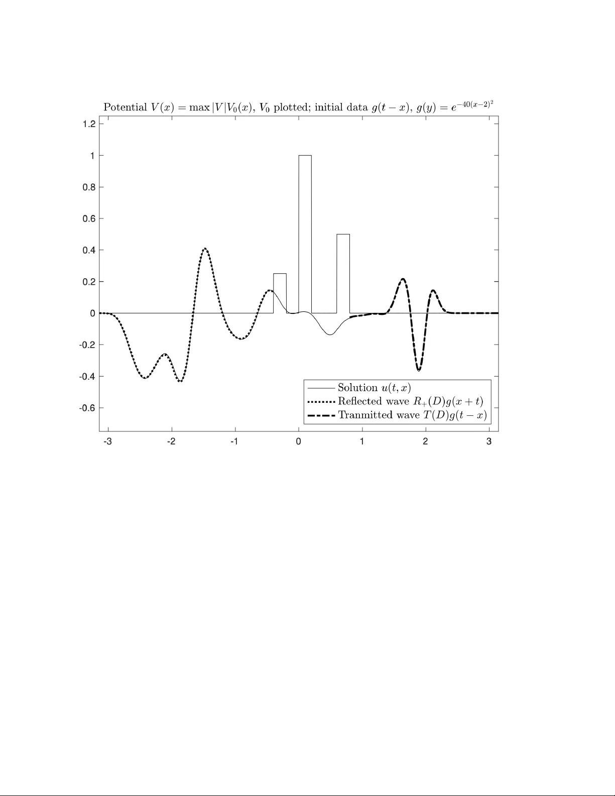
1D SCA TTERING THR OUGH TIME DEPENDENT MEDIA WITH MEMOR Y JEFFREY GALK OWSKI AND MA CIEJ ZW ORSKI With an appendix by Zhen Huang and Ma ciej Zworski Abstract. W e construct a scattering matrix with op erator v alued e n tries describing solutions to the 1+1 w av e equation where permittivities has memory and dep ends on time and space. It is the analogue of the scattering matrix for spatially lo calised p erturbations where the en tries are functions of frequency and appear as F ourier mul- tipliers in solutions of the wa v e equation. This provides a mathematical explanation of the n umerical construction in the recent pap er by Horsley et al [ HGW23 ]. 1. Introduction There is a considerable in terest in materials whose properties dep end on time and whic h ha v e memory . Ha ving memory essentially means having a (causal) dep endence on frequency – see for instance [ Ga ∗ 22 ] for a surv ey and [ Ga ∗ 26 ] for a recen t experimen- tal and theoretical study . Our motiv ation comes from a letter [ HGW23 ] b y Horsley , Galiffi, and W ang and w e refer to it for more references to the literature and the ph ysics bac kground. 1.1. Scattering for p ermittivities with memory. D 2 t u ( t, x ) − a ( x, t ) Z t −∞ e − γ ( t − t ′ ) D t u ( t ′ , x ) dt ′ − D 2 x u ( t, x ) = 0 , , a ∈ L ∞ ( R x ; C ∞ c ( R t )) , supp a ⊂ [ − R, R ] × [ − T , T ] , γ > 0 , u ( t, x ) | t ≤ 0 = g ( x − t ) , supp g ⊂ ( −∞ , − R ) . (1.1) (The compact supp ort in time could b e relaxed to sup erexp onen tial decay but w e restrict ourselv es to the simplest case here). A t least formally this corresp onds on the F ourier transform side to P := D 2 x − ω 2 + A ( x ) , A ( x ) := a ( x, D ω ) ω ω + iγ : H r ( R ω ) → H r ( R ω ) , (1.2) where H α :=  f : f ( • ) ∈ O ( C + ) , sup σ > 0 e − 2 σ α Z R | f ( λ + iσ ) | 2 dλ < + ∞  , (1.3) 1 2 JEFFREY GALKO WSKI AND MA CIEJ ZWORSKI Figure 1. Comparisons of ev olutions of a gaussian pac ket g ( t − x ), t ≪ 1, g ( y ) = e − ( x 0 + y ) 2 ) /σ − iλ ( y − x 0 )) , σ = 0 . 05, λ = 10, x 0 = − 2 for dif- feren t v alues of the parameters in ( 2.9 ) (with m = 1) – this corresp onds to the mo del considered in [ HGW23 ]. An animated version is a v ail- able at https://math.berkeley.edu/ ~ zworski/wave_multi_one.mp4 . The co de for pro ducing this mo vie and the figure is enclosed in the ap- p endix. and also write H ∞ := ∪ α H α . The Hardy spaces H α app ear naturally in scattering theory for the wa ve equation since the w ork of Lax–Phillips [ LP68 ] – see § 3.1 , and ( 3.6 ) specifically , for the review of the simplest case. The action of a ( x, D ω ) is given by [ a ( x, D ω ) u ]( x, ω + iσ ) := 1 2 π Z \ a ( x, • )( ω − λ ) u ( x, λ + iσ ) dλ. (1.4) 1D SCA TTERING THR OUGH TIME DEPENDENT MEDIA WITH MEMOR Y 3 W e in tro duce the follo wing Hilb ert space of functions of p osition and frequency , f : R × C + → C , C + := { ω ∈ C : Im ω > 0 } , H s α :=  f : f ( x, • ) ∈ O ( C + ) , sup σ > 0 e − 2 σ α Z R ∥ f ( · , λ + iσ ) ∥ 2 H s ( R ) dλ < + ∞  . (1.5) W e write H α := H 0 α , H ∞ = ∪ α H α , and H s α, loc : { u : u ( x, • ) ∈ O ( C + ) and χ ( x ) u ( x, ω ) ∈ H s α for all χ ∈ C ∞ c } . The goal now is to pro ve the following analogue of the existence of the scattering matrix ( 3.2 ): Theorem 1. Supp ose that assumptions in ( 1.1 ) hold and f ∈ ( ω + i ) − 1 H − R . Then ther e exist b ounde d op er ators T , R + : ( ω + i ) − 1 H α → ω − 1 H α +2 R , α ∈ R , such that, for P given in ( 1.2 ) , ther e exists a unique solution, u ( x, ω ) ∈ ω − 1 H ∞ , loc , ( x, ω ) ∈ R 2 , of P u = 0 such that u ( x, ω ) =  f ( ω ) e iω x + R + f ( ω ) e − iω x , x < − R , T f ( ω ) e iω x , x > R. (1.6) The operators R + and T were constructed n umerically in [ HGW23 ] for the case when a ( x, t ) = V 0 1 l − R,R ( x ) χ ( t ). That was done b y following the construction of the scattering matrix for step p otentials (see § 3.1 and [ DyZw19 , Exercise 2.10.6]) but with the exponentials e ± ω x for | x | > R and e ± i √ ω 2 − V 0 x for | x | < R , replaced Schr¨ odinger propagators e ± ixχ ( D ω ) ω / ( ω + iγ ) for | x | < R . The needed inv ersion of op erators was established n umerically . The p oint of Theorem 1 is that, under the assumption of lo calisation in space and time, the op erator exists even for a larger class of perturbations. The pro of has t wo parts: the first, in § 3.2 , is a functional analytic setup for con- structing u ( x, ω ). The second one, in § 3.3 , is the pro of of non-existence of purely outgoing solutions to P u = 0, that is solutions satisfying ( 1.6 ) with f ≡ 0 but the terms corresponding to R + f and T f p otentially nonzero. 1.2. The w a v e equation. W e now describ e how the op erators constructed in Theo- rem 1 app ear in the w av e evolution. The theorem in the exact analogue of Prop osition 4 in which the standard scattering matrix for compactly supp orted 1D p oten tials ap- p ears in the description of scattered wa ves. 4 JEFFREY GALKO WSKI AND MA CIEJ ZWORSKI Theorem 2. Supp ose that g ∈ C ∞ c (( R, ∞ )) and that u ( t, x ) is the unique solution of ( 1.1 ) satisfying u ( t, x ) = g ( t − x ) , t < 0 . Then u ( t, x ) =  g ( t − x ) + R + g ( x + t ) , x < − R, T g ( t − x ) , x > R, (1.7) wher e d R + g ( ω ) := R + b g ( ω ) , d T g ( ω ) := T b g ( ω ) . and T and R + ar e describ e d in The or em 1 . Existence of op erators R + and T (under some assumptions guaranteeing existence and uniqueness of solutions to the wa ve equation) is an elementary general fact – see Prop osition 1 . The p oint here is these op erators are related to the stationary problem from Theorem 1 and ha v e correct mapping prop erties. At this stage, we provide the co des for solving the wa ve equation (see the App endix and Figure 1 ) but not the comparison with the scattering matrix. It is an interesting op en question, relev ant to ph ysics problems considered in [ HGW23 ] and references given there, to analyse quan titativ e prop erties of R + and T in asymptotic regimes of the parameters. The n umerical exp eriments (whic h an in terested reader is invited to p erform using co de in the Appendix) indicate in teresting phenomena whic h should inv estigated. Ac kno wledgemen ts . JG ac know ledges supp ort from EPSRC gran ts EP/V001760/1 and EP/V051636/1, the Lev erh ulme T rust under Research Pro ject Grant RPG-2023- 325, and the ERC under the Synergy grant PSINumScat 101167139. and MZ from the Simons F oundation under a “Moir´ e Materials Magic” grant. W e are also grateful to S.A.R. Horsley for discussions about ph ysical motiv ation and to Bryn Da vies for useful references. The second author w ould also like to thank H. Ammari for his hospitality in Zurich where he first learned ab out time dep endent materials with memory , and Univ erisit y College, London, for providing supp ort during his visit there. 2. General theor y W e discuss a general definition of a scattering op erator for spatially lo calised p er- turbations of the 1+1 w a v e equation. W e then define a general class of p erturbations with time dep endence and memory and prov e existence and uniqueness for the cor- resp onding wa ve equation. These preliminary results are not surprising but we not seem to ha v e a ready to use reference cov ering existence and uniqueness of the Cauch y problem for op erators describ ed in § 1 and for the more general ones given in ( 2.5 ). W e present a detailed argumen t in our sp ecific case noting that it generalises to higher dimensions. 1D SCA TTERING THR OUGH TIME DEPENDENT MEDIA WITH MEMOR Y 5 2.1. An abstract scattering op erator. The following elementary result shows that w e can define the scattering matrix for very general spatially lo calised p erturbations (see § 3.1 for a review of the standard theory in our context). Supp ose that P : D ′ ( R 2 ) → D ′ ( R 2 ) has the prop erty that u ∈ D ′ ( R 2 ) , supp u ∩ ( R × [ − R , R ]) = ∅ = ⇒ P u = D 2 x u. (2.1) More informally we can state this as ∀ t ∈ R supp u ( t, • ) ∩ [ − R, R ] = ∅ = ⇒ P u ( t, x ) = D 2 x u ( t, x ) . W e do not assume that P is linear here. F or a general class of linear op erators P relev an t to this note, see § 2.2 . Under this assumption on P we ha ve the follo wing simple fact: Prop osition 1. Supp ose that u ∈ D ′ ( R 2 ) solves ( D 2 t − P ) u = 0 and u | t< 0 = κ ∗ + g | t< 0 , κ ± : R 2 → R , κ ± ( t, x ) := t ∓ x, g ∈ D ′ ( R ) , supp g ⊂ ( −∞ , − R ) . Then ther e exist G, F ∈ D ′ ( R ) , supp G, supp F ⊂ ( − R, ∞ ) , such that u | x< − R = κ ∗ + g | x< − R + κ ∗ − G | x< − R , u | x>R = κ ∗ + F | x>R . (2.2) Less formally the hypothesis reads as u ( t, x ) = g ( t − x ) , t < 0 , supp g ⊂ ( −∞ , − R ) , (2.3) and the conclusion as u ( t, x ) =  g ( t − x ) + G ( t + x ) , x < − R, supp G ⊂ ( − R , ∞ ) , F ( t − x ) , x > R, supp F ⊂ ( −∞ , R ) . (2.4) This means that under the assumption ( 2.1 ) and provided we ha ve existence and uniqueness to solutions of ( D 2 t − P ) u = 0, we hav e scattering maps: g 7→ T g := F , g 7→ R + g = G, where T and R + are transmission and reflection maps. (W e ha v e similar definitions for w a ves g approac hing from the right.) As explained in § 1 this pap er describ es mapping prop erties and basic structure of T and R + for more sp ecific p erturbations and relates them to stationary scattering theory . Pr o of of Pr op osition 1 . W e first pro ceed by pretending that u is a function and take r > R . If we write z = t − x and w = x + t so that for v ( z , w ) = u ( x, t ) w e hav e ∂ z ∂ w v = 0 for ± ( w − z ) > 2 r . In particular, ∂ z ∂ v v ( z , w ) = 0 for − z > 2 r − w , that is 6 JEFFREY GALKO WSKI AND MA CIEJ ZWORSKI ∂ w v ( z , w ) = f ( w ), w > 2 r + z for some f defined for all v alues of w . But that means that v ( z , w ) = v ( z , 2 r + z ) + Z 0 2 r + z f ( y ) dy + Z w 0 f ( y ) dy , for w − z > 2 r , that is v ( z , w ) = G + ( z ) + F + ( w ) for w − z > 2 r . Similarly , v ( z , w ) = G − ( z ) + F − ( w ) for w − z < − 2 r . This argumen t applies to distributions by using [ H¨ o03 , Theorem 3.1.4 ′ ] and the fact that the restriction of v to L := { ( z , 2 r + z ) : z ∈ R } is well defined as for w − z > 2 R , WF( v ) ⊂ { ( z , w ; ζ , ω ) : ζ ω = 0 } whic h (aw ay from the zero section) is disjoin t from N ∗ L = { ( z , 2 r − z , ζ , ζ ) : z , ζ ∈ R } – see [ H¨ o03 , Corollary 8.2.7]. Since r > R is arbitrary we can replace r with R in our conclusion. W e now need to pro v e that G + ≡ 0 and G − = g . T o see the first claim w e note that ( 2.3 ) gives F + ( z ) + G + ( w ) = 0 for w − z = 2 x > 2 R and w + z = 2 t < 0. In particular, G ′ + ( w ) = 0 for 2 R + z < w < − z , and as z is arbitrary , this shows that G + is constant. W e can absorb that constant into F + and hence hav e G + ≡ 0. T o see that G − = g , w e note that ( 2.3 ) giv es G − ( z ) − g ( z ) + F − ( w ) = 0 for w − z = 2 x < − 2 R and w + z = 2 t < 0. Hence G ′ − ( z ) − g ′ ( z ) = 0 for w < − z < − 2 R − w . Since w is arbitrary , this means that G − ( z ) − g ( z ) is constan t and w e can make it 0 b y c hanging F − . □ 2.2. A class of p ermittivities. The mo del we consider is the wa ve equation with p ermittivit y whic h dep ends on time but also has memory in the sense of b eing an op er- ator. In this section w do not assume spatial lo calisation and consider a generalisation of ( 1.1 ): P := ∂ t ε∂ t − ∂ 2 x , x ∈ R , εv ( t, x ) := v ( t, x ) + B v ( t, x ) , B v ( t, x ) := Z t −∞ B ( x, t, t − t ′ ) v ( t ′ , x ) dt ′ . (2.5) W e t ypically w an t to solv e the problem P v = F ( t, x ) , supp F ⊂ ( − R, ∞ ) × R , v ( t, x ) | t< − R = 0 . (2.6) W e mak e the follo wing assumptions on B :and that there exists m and m 0 suc h that ∀ k , ℓ ∃ C kℓ | ∂ k t ∂ ℓ s B ( x, t, s ) | ≤ C kℓ ⟨ t ⟩ m 0 ⟨ s ⟩ m . (2.7) Later, but not in this section, we assume that w e ha v e a lo calisation in space, that is, for R > 0 indep enden t of t and s supp B ( • , t, s ) ⊂ ( − R, R ) (2.8) As an example we can tak e B ( x, t, s ) = V ( x ) e − αt 2 e − γ s s m , α, γ ≥ 0 , V ∈ L ∞ ( R ) , (2.9) 1D SCA TTERING THR OUGH TIME DEPENDENT MEDIA WITH MEMOR Y 7 noting that the case of α = γ = 0, m = 1, giv es P = ∂ 2 t − ∂ 2 x + V ( x ). Another w ay of writing the op erator B in ( 2.9 ) is as a pseudo differen tial op erator: B = b ( x, t, D t ) , b ( x, t, τ ) := V ( x ) e − αt 2 i m ( τ + iγ ) − m , a ( t, D t ) h := Z R a ( t, τ ) b h ( τ ) dτ , h ( t ) = 1 2 π Z R b h ( ω ) e − iω t dω . (2.10) W e note here that our conv ention for F ourier transform in time is non-standard but leads to cleaner formulas in our setting. The most relev ant case for us is ( 1.1 ). F or that we take B ( x, t, s ) = γ − 1 ( e − sγ − 1) a ( x, t ) , γ > 0 , a ∈ L ∞ x C ∞ t , supp a ⊂ [ − R, R ] × [ − T , T ] . (2.11) In that case we ha ve m 0 = −∞ , m = 1 . (This means that in ( 2.13 ) b elo w w e can tak e γ ( T ) ≡ 1.) Since we do not know a ready to use reference cov ering existence and uniqueness of the Cauch y problem for P in ( 2.5 ) we present a detailed argumen t in our sp ecific case noting that it generalises to higher dimensions. 2.3. Existence and uniqueness. The result of § 2.1 is applicable to op erators of the form ( 2.5 ) thanks to the follo wing Prop osition 2. Under the assumptions ( 2.5 ) and ( 2.7 ) , for F ∈ L 1 ([0 , T ]; L 2 ( R )) , ther e exists a unique u ∈ C (( −∞ , T ]); H 1 ( R )) ∩ C 1 (( −∞ , T ]); L 2 ( R )) , supp u ⊂ [0 , T ] , (2.12) such that P u = F on (0 , T ) × R Mor e over, ther e exists C 0 , λ > 0 (indep endent of T ) such that for 0 ≤ t ≤ T . ∥ u ( t, • ) ∥ H 1 ( R ) + ∥ ∂ t u ( t, • ) ∥ L 2 ( R ) ≤ C 0   e λγ ( T )( T − t ′ ) F ( t ′ , x )   L 2 (0 ,T ) t ′ × R x ) , γ ( T ) := 1 + ⟨ T ⟩ m 0 +1 + ⟨ T ⟩ m 0 + m +1 . (2.13) T o obtain uniqueness and ( 2.13 ) we will use Lemma 3. Supp ose that ( 2.12 ) is satisfie d and that in addition, F := P u ∈ L 1 ([0 , T ]; L 2 ( R )) . Then ( 2.13 ) holds. 8 JEFFREY GALKO WSKI AND MA CIEJ ZWORSKI Pr o of. This is done by an adaptation of the usual energy estimate based on the energy iden tit y (see for instance [ H¨ o85 , (2.4.2)] for a v ery general v ersion): ∂ t ( e − 2 λt 1 2 ( | u t | 2 + |∇ x u | 2 + | u | 2 )) − ∇ x · (Re ∇ x u ¯ u t ) + λe − 2 λt ( | u t | 2 + |∇ x u | 2 + | u | 2 ) = − 2 Im e − 2 λt P uD t u − e − 2 λt D t B D t uD t u − e − 2 λt µ 2 uD t u + e − 2 λt Re u ¯ u t . Supp ose u ∈ H 1 (( −∞ , T ) × R ) with supp u ⊂ [0 , T ] and P u ∈ L 2 . Then, in tegrating the energy identit y on ( −∞ , T ) × R , using the diverg ence theorem (in higher dimen- sions), the fact that the form of B in ( 2.5 ) implies supp B D t u ⊂ ( −∞ , T ], and that for supp v ⊂ [0 , T ], Z T −∞    e − λt D t Z t 0 B ( x, t, t − t ′ ) e λt ′ v ( t ′ , x ) dt ′    2 L 2 x dt ≤ C Z T 0 ⟨ t ⟩ 2 m 0 ∥ v ( t, • ) ∥ 2 L 2 x dt + C Z T 0 ⟨ t ⟩ 2 m 0 (1 + ⟨ t ⟩ 2 m ) ∥ v ∥ 2 L 1 ((0 ,t ); L 2 x ) dt ≤ C γ ( T ) 2 ∥ v ∥ 2 L 2 , where γ ( T ) is defined in ( 2.13 ). F rom this w e obtain e − 2 λT 1 2 ( ∥ u t ( T ) ∥ 2 L 2 ( R ) + ∥ u ( T ) ∥ 2 H 1 ( R ) ) + λ ( ∥ e − λt u ∥ 2 L 2 (( −∞ ,T ); H 1 ( R )) + ∥ e − λt u t ∥ 2 L 2 (( −∞ ,T ) × R ) ) = − 2 Im ⟨ e − λt P u, e − λt D t u ⟩ ( −∞ ,T ) × R − ⟨ e − λt D t B e λt e − λt D t u, e − λt D t u ⟩ L 2 (( −∞ ,T ) × R ) −⟨ e − λt µ 2 e λt e − λt u, e − λt D t u ⟩ ( −∞ ,T ) × R + Re ⟨ e − λt u, e − λt ∂ t u ⟩ ≤ C ∥ e − λt f ∥ 2 L 2 (( −∞ ,T ) × R ) + ( C 0 γ ( T ) 2 + 1) ∥ e − λt D t u ∥ 2 L 2 (( −∞ ,T ) × R ) + 1 2 ∥ e − λt u ∥ 2 L 2 (( −∞ ,T ) × R ) . Hence, taking λ large enough, and moving the t wo righ t-most terms to the left-hand side, w e obtain ( 2.13 ) (with λγ ( T ) replacing λ ). □ Pr o of of Pr op osition 2 . Uniqueness is immediate from Lemma 3 and ( 2.13 ). It remains to sho w existence. F or that w e will use the free w av e group, U ( t ) : H s ( R ) × H s − 1 ( R ) → H s ( R ) × H s − 1 ( R ): U ( t ) =:  cos( D x t ) sin( D x t ) /D x − D x sin( D x t ) cos( D x t )  = e tL , L :=  0 I − D 2 x 0  , D x := (1 /i ) ∂ x . (2.14) W e fix T − ≥ 0 and for w ∈ C 0 (( −∞ , T − ); H 1 × L 2 ) , supp w ⊂ [0 , T ] × R , (2.15) define a sequence v n ( t ) ∈ C 0 (( −∞ , T ); H 1 × L 2 ) , n = − 1 , 0 , · · · , supp v n ⊂ [0 , T ] × R , (2.16) 1D SCA TTERING THR OUGH TIME DEPENDENT MEDIA WITH MEMOR Y 9 inductiv ely as follows: v − 1 := ( w ( t ) t ≤ T − , w ( T − ) T − ≤ t ≤ T . Then for n ≥ 0, w e again define v n differen tly in different ranges of t . F or t ≤ T − w e put v n ( t ) := w ( t ), while for T − ≤ t ≤ T , v n ( t ) := U ( t − T − ) w ( T − ) + Z t T − U ( t − s )  0 F ( s )  −  0 0 µ 2 ∂ t B  v n − 1 ( s ) ! ds. (2.17) Then ( 2.16 ) holds and ( ∂ t − L ) v n =  0 F  −  0 0 µ 2 ∂ t B  v n − 1 , t ∈ ( T − , T ) v n ( T − ) = w ( T − ) . In particular, ( ∂ t − L )( v n − v n − 1 ) = −  0 0 µ 2 ∂ t B   v n − 1 − v n − 2  , t ∈ ( T − , T ) , v n ( T − ) − v n − 1 ( T − ) = 0 . (2.18) W e no w observ e that ( 2.5 ) and ( 2.7 ) sho w that for v ∈ C 0 (( −∞ , T ); L 2 ), supp v ⊂ [0 , T ] × R ∥ ∂ t B v ( s ) ∥ 2 L 2 ( R ) ≤ Z R     Z s 0 ⟨ s ⟩ m ⟨ s − t ′ ⟩ m 0 v ( t ′ , x ) dt ′     2 dx ≤ ⟨ s ⟩ 2 m (1 + ⟨ s ⟩ 2 m 0 ) ∥ v ∥ 2 L 1 ((0 ,s ); L 2 )) . (2.19) Since v n − 2 ( t ) − v n − 1 ( t ) = 0 for t < T − it follo ws from ( 2.17 ) that ∥ v n ( t ) − v n − 1 ( t ) ∥ H 1 × L 2 ≤ C Z t T − (1 + | t − s | )( ∥ v n − 1 ( s ) − v n − 2 ( s ) ∥ H 1 × L 2 + ⟨ s ⟩ m (1 + ⟨ s ⟩ m 0 ) ∥ v n − 1 − v n − 2 ∥ L 1 ( T − ,s ); H 1 × L 2 ) ds, for some constant C . Using T − + δ ≤ T + 1, w e see that for δ < 1, there is a new constan t C 1 dep ending on T but not on T − , ∥ v n − v n − 1 ∥ L ∞ (( T − ,T − + δ ); H 1 × L 2 ) ≤ C (1 + ⟨ T − + δ ⟩ m (1 + ⟨ T − + δ ⟩ m 0 ) δ ) ∥ v n − 1 − v n − 2 ∥ L 1 (( T − ,T − + δ ); H 1 × L 2 ) ≤ C 1 δ ∥ v n − 1 − v n − 2 ∥ L ∞ (( T − ,T − + δ ); H 1 × L 2 ) T aking δ < 1 /C 1 , we concluded that v n is a Cauc hy sequence in L ∞ (( T − , T − + δ ); H 1 × L 2 ). Since v n ( t ) = w ( t ) for t ≤ T − , v n ∈ C 0 ([ T − , T − + δ ]; H 1 × L 2 ) , v n ( T − ) = w ( T − ) , v n con v erges to v ∈ C 0 (( −∞ , T − + δ ]; H 1 × L 2 ) and v | ( −∞ ,T − ) = w | ( −∞ ,T − ) . 10 JEFFREY GALKO WSKI AND MA CIEJ ZWORSKI In particular we ha ve conv ergence v n ( t ) → v ( t ) in the sense of distributions on ( T − , T − + δ ), and hence, from ( 2.17 ), in the sense of distributions, ∂ t v = L v −  0 0 µ 2 ∂ t B  v +  0 F  , on ( T − , T − + δ ) × R . Putting v = [ v 1 , v 2 ] t , this giv es ∂ t v 1 = v 2 ∈ C 0 ([ T − , T − + δ ]; L 2 ). Hence u := v 1 , satisfies u ∈ C 0 (( −∞ , T + + δ ]; H 1 ) ∩ C 1 ( −∞ , T − + δ ]) , u ( T − ) = w 1 ( T − ) , ∂ t u ( T − ) = w 2 ( T − ) , w =: [ w 1 , w 2 ] t , P u = F in the sense of distributions on ( T − , T − + δ ). (2.20) The only conditions here are ( 2.15 ) on w and and δ > 0. W e can no w pass from this small step pro cedure to finding u ∈ C 0 (( −∞ , T ); H 1 ( R )) ∩ C 1 (( −∞ , T ); L 2 ( R )) , supp u ⊂ [0 , T ] , satisfying P u = F on (0 , T ). T o do this, we set u 0 = 0 and for j ≥ 1 and use ( 2.20 ) to inductiv ely obtain u j ∈ C 0 (( −∞ , j δ ]; H 1 ( R )) ∩ C 1 (( −∞ , j δ ]; L 2 ( R )) , (2.21) satisfying P u j = F , distributionally on (( j − 1) δ, j δ ) × R , u j (( j − 1) δ ) = u j − 1 (( j − 1) δ ) , ∂ t u j (( j − 1) δ ) = ∂ t u j − 1 (( j − 1) δ ) . (2.22) W e claim that P u j = F distributionally on (0 , j δ ) . (2.23) Indeed, supp ose b y induction that this holds for j replaced b y j − 1. Then, ( 2.21 ) holds and P u j = F distributionally on ((0 , ( j − 1) δ ) ∪ (( j − 1) δ, j δ ) . W e w e write P = ∂ 2 t − L u , L u := ∂ 2 x u − ∂ t B ∂ t u − µ 2 u , then G := L u ∈ C 0 (( −∞ , j δ ); H − 1 ) , and hence, with H := F + G , ∂ 2 t u = H ∈ C 0 (( −∞ , j δ ); H − 1 ) distributionally on ((0 , ( j − 1) δ ) ∪ (( j − 1) δ , j δ ) . But the con tin uity of u and ∂ t u across ( j − 1) δ shows that the equation holds distribu- tionally on (0 , j δ ). (The argument reduces to showing that if g , G ∈ C 0 and ∂ t g = G , on R \ { 0 } then ∂ t g = G on R . But that follows from testing against φ ( t )(1 − χ ( t/ε )) where φ, χ ∈ C ∞ c ( R ), χ ≡ 1 near 0, and using contin uity of g and G while letting ε → 0.) T aking J ≥ δ − 1 T and setting u = u J completes the construction of u . □ 1D SCA TTERING THR OUGH TIME DEPENDENT MEDIA WITH MEMOR Y 11 Figure 2. An illustration of Prop osition 4 : the solution to ( ∂ 2 t − ∂ 2 x + V ( x )) u = 0, supp V ⊂ [ − R , R ], with u ( t, x ) = g ( t − x ) for t ≪ − 1 is giv en b y g ( t − x ) + R + ( D ) g ( t + x ) for x ≤ − R and T ( D ) g ( t − x ) for x ≥ R (for all times; t = 4 shown). An animated v ersion is av ailable at https://math.berkeley.edu/ ~ zworski/wave_pot.mp4 . 3. An opera tor v alued sca ttering ma trix In this section w e prov e Theorem 1 . T o motiv ate the construction and to link it to standard theory w e first review the case compactly supp orted time indep enden t p oten- tials (the case α = γ = 0 and m = 1 in § 2.2 ) . The w av e equation setting (unlik e the more common Schr¨ odinger equation setting) makes the the scattering matrix app ear in a very clean w ay . 3.1. Review of standard scattering matrix. Supp ose that V ∈ L ∞ ( R ; R ) satisfies supp V ⊂ [ − R, R ]. Any solution to ( D 2 x + V ( x ) − λ 2 ) u = 0 , (3.1) 12 JEFFREY GALKO WSKI AND MA CIEJ ZWORSKI satisfies u ( x ) =  A + e iλx + B − e − iλx , x > R ; A − e iλx + B + e − iλx , x < − R . T aking the W ronskian of u and ¯ u for λ ∈ R \ 0 shows that | A − | 2 + | B − | 2 = | A + | 2 + | B + | 2 , and hence S ( λ ) :  A − B −  7→  A + B +  , S ( λ ) =  T ( λ ) R − ( λ ) R + ( λ ) T ( λ )  , (3.2) is well defined. It is called the sc attering matrix , T ( λ ) is the transmission co efficien t and R ± ( λ ) are the reflection co efficien ts. They extend to mer omorphic functions in C satisfying T ( λ ) T ( ¯ λ ) + R ± ( λ ) R ± ( ¯ λ ) = 1 , T ( λ ) R ± ( λ ) + R ± ( λ ) T ( ¯ λ ) = 0 , T ( − λ ) = T ( ¯ λ ) , R ± ( − λ ) = R ± ( ¯ λ ) , (3.3) and N Y j =1 | λ − iµ j | | λ + iµ j | | T ( λ ) | ≤ e 2 R Im λ , N Y j =1 | λ − iµ j | | λ + iµ j | | R ± ( λ ) | ≤ e 2 R Im λ , Im λ ≥ 0 , (3.4) where µ j > 0 and − µ 2 j , j = 1 , · · · , N , are the eigenv alues of D 2 x + V ( x ) – see [ DyZw19 , § 2.4, Exercise 3.14.10]. The normalised eigenfunctions w j ∈ L 2 ( R ; R ) satisfy ( D 2 x + V ( x )) w j = − µ 2 j w j , ∥ w j ∥ L 2 = 1 , w j ( x ) | ± x>R = a ± j e ∓ µ j x , µ j > 0 . (3.5) When V ≥ 0 there are no eigen v alues and in that case w e can consider m ultiplication b y T and R ± on Hardy spaces: H α := { f ∈ O ( { Im λ > 0 } ) : sup σ > 0 e − 2 aσ Z R | f ( λ + iσ ) | 2 dλ < + ∞} , H α ∋ f ( λ ) 7→ T ( λ ) f ( λ ) ∈ H a +2 R , H α ∋ f ( λ ) 7→ R ± ( λ ) f ( λ ) ∈ H a +2 R . (3.6) W e remark that the spaces are isometric as f ( ω ) 7→ e iaω f ( ω ) pro vides a unitary map b et w een H α and H . The relation to the w a ve equation is giv en in the follo wing Prop osition 4. Supp ose that g ∈ S ′ ( R ) and that supp g ⊂ ( R , ∞ ) . If ( D 2 t − D 2 x − V ( x )) u ( t, x ) = 0 , t ∈ R , u ( t, x ) = g ( t − x ) , t ≤ 0 , (3.7) then, in the notation of ( 3.2 ) and ( 3.5 ) , u ( t, x ) =  g ( t − x ) + M − g ( x + t ) , x < − R, M + g ( t − x ) , x > R, (3.8) 1D SCA TTERING THR OUGH TIME DEPENDENT MEDIA WITH MEMOR Y 13 wher e M − g ( x ) = R + ( D ) g ( x ) + N X j =1 ⟨ g , w j ⟩ a − j e µ j x , M + g ( x ) = T ( D ) g ( x ) + N X j =1 ⟨ g , w j ⟩ a + j e µ j x , and wher e T and R + ar e define d in ( 3.2 ) . Remark. A t first it is not clear that the expression in ( 3.8 ) has the desired supp ort prop erties. T o see this when there are no eigenv alues, we first note that by the Paley– Wiener Theorem b g ( λ ) (with the con v en tion of ( 2.10 )) is holomorphic for Im λ > 0 and satisfies the b ound ⟨ λ ⟩ N e − ( R + δ ) Im λ , δ > 0, there. In view of ( 3.4 ) we then ha v e T ( λ ) b g ( λ ) , R + ( λ ) b g ( λ ) = O ( ⟨ λ ⟩ N ) e ( R − δ ) Im λ , Im λ > 0 . The P aley–Wiener Theorem then shows that supp T ( D ) g , supp R + ( D ) g ⊂ ( − R , ∞ ) and supp 1 l −∞ , − R ) ( • ) R + ( D ) g ( • + t ) ∩ ( −∞ , R ) ⊂ { x : − t − R < x < − R } , supp 1 l ( R, ∞ ) T ( D ) g ( t − • ) ∩ ( R , ∞ ) ⊂ { R < x < t + R } . In particular for t ≤ 0 the scattering terms b oth v anish. When there are eigenv alues, − µ 2 j , then the en tries of S ( λ ) hav e p oles iµ j , µ j > 0. A contour deformation then pro vides the needed cancellation. Pr o of. W e use the sp ectral representation of the wa ve propagator constructed using distorted plane wa ves, that is solutions to ( D 2 x + V − λ 2 ) e ± = 0 satisfying e ± ( x, λ ) = ( T ( λ ) e ± iλx for ± x > R , e ± iλx + R ± ( λ ) e ∓ iλx for ± x < − R . (3.9) Then, for g ∈ C ∞ c ( R ), supp g ⊂ ( R, ∞ ), u ( t, x ) = N X j =1 ( ⟨ g , w j ⟩ cosh µ j t − ⟨ g ′ , w j ⟩ µ − 1 j sinh µ j t ) w j ( x ) + 1 2 π Z ∞ 0 Z R ( e + ( x, λ ) e + ( y , λ ) + e − ( x, λ ) e − ( y , λ ))(cos tλ − λ − 1 sin tλ∂ y ) g ( − y ) dy dλ. In view of the supp ort prop erties of g and the form of w j for x < − R we hav e ⟨ g ′ , w j ⟩ = Z g ′ ( x ) a − j e xµ j dx = − µ j Z g ( x ) a − j e xµ j dx = − µ j ⟨ g , w j ⟩ . 14 JEFFREY GALKO WSKI AND MA CIEJ ZWORSKI Hence the contribution of w j ’s to u ( t, x ) is giv en b y N X j =1 e tµ j ⟨ g , w j ⟩ w j ( x ) = N X j =1 a ± j ⟨ g , w j ⟩ e µ j ( t ∓ x ) , ± x > R. T o see the con tribution of the con tin uous sp ectrum, w e no w use the expressions for e ± ( y , λ ) for y < − R : E + g ( λ, t ) := Z R e + ( y , λ )(cos tλ − λ − 1 sin tλ∂ y ) g ( − y ) dy = b g ( λ ) e − iλt + R + ( λ ) b g ( − λ ) e iλt , E − g ( λ, t ) := Z R e − ( y , λ )(cos tλ − λ − 1 sin tλ∂ y ) g ( − y ) dy = T ( λ ) b g ( − λ ) e iλt . (3.10) Then for x < − R , e + ( x, λ ) E + g ( λ, t ) = ( e iλx + R + ( λ ) e − iλx )( b g ( λ ) e − iλt + R + ( λ ) b g ( − λ ) e iλt ) = b g ( λ ) e iλ ( x − t ) + | R + ( λ ) | 2 b g ( − λ ) e iλ ( t − x ) + R + ( λ ) e − iλ ( x + t ) b g ( λ ) + R + ( − λ ) e iλ ( x + t ) b g ( − λ ) e iλ ( t − x ) , e − ( x, λ ) E − g ( λ, t ) = | T ( λ ) | 2 b g ( − λ ) e − iλ ( x − t ) . Using ( 3.3 ) in the expression for u ( t, x ) gives ( 3.8 ) for x < − R . Similar argumen ts giv e the expression for x > R . □ 3.2. Construction of u ( x, ω ) in Theorem 1 . T o motiv ate the construction of u ( x, ω ) w e recall one wa y to do it in the case of ( 3.1 ). F or V ∈ L ∞ comp ( R ; [0 , ∞ )), supp V ⊂ ( − R, R ), we consider the resolven t R V ( ω ) := ( D 2 x + V − ω 2 ) − 1 : L 2 ( R ) → L 2 ( R ) whic h is holomorphic for Im ω > 0. When V ≡ 0 (note we assumed that V ≥ 0), it is defined L 2 comp ( R ) → L 2 loc ( R ) for Im ω = 0. (See [ DyZw19 , Theorem 2.7].) F or F with supp F ⊂ ( − R 1 , R 1 ), R < R 1 , R V ( ω ) F ( x ) =  A − ( ω ) e − iω x , x < − R 1 , A + ( ω ) e iω x , x > R 1 , (3.11) whic h is the meaning of b eing outgoing for 1D for compactly supp orted p erturbations. (Here A ± dep end on F and ω .) T o construct a solution of ( D 2 x + V − ω 2 ) u = 0 satisfying ( 1.6 ) we c ho ose ρ ∈ C ∞ c ( R ; [0 , 1]) supp orted in ( − R 1 , R 1 ), R 1 > R , and equal to 1 near the support of V . W e then put u ( x, ω ) = (1 − ρ ( x )) e iω x f ( ω ) + R V ( ω )[ D 2 x , ρ ]( e i • ω f ( ω ))( x ) , Then ( 3.11 ) sho ws that ( 1.6 ) holds. W e will mimic this strategy and construct R V ( ω ) no w acting on spaces of functions of b oth x and ω . The key is the existence of R V in H α whic h will b e established in § 3.3 . W e start b y recording some simple facts: 1D SCA TTERING THR OUGH TIME DEPENDENT MEDIA WITH MEMOR Y 15 Lemma 5. F or R 0 ( ω ) = ( D 2 x − ω 2 ) − 1 , Im ω > 0 , the outgoing r esolvent, and 0 ≤ s ≤ 2 , define R s : f ( x, ω ) 7→ ω ( ω + i ) s R 0 ( ω ) f ( • , ω )( x ) . (3.12) Then, in the notation of ( 1.5 ) , for ρ ∈ C ∞ c ( R ) , and any α ∈ R , ∥ ρ R s ρ ∥ H α → H s α ≤ C, ρ R s ρf ( x, ω ) := ρ ( x ) ω ( ω + i ) − s R 0 ( ω )( ρ ( • ) f ( • , ω ))( x ) . (3.13) Pr o of. This follows immediately from he definition ( 1.5 ) and the explicit formula for R 0 ( ω ) as an op erator L 2 comp ( R ) → H 2 loc ( R ): ω ( ω + i ) s R 0 ( ω ) g ( x ) = i 2( ω + i ) s Z R e iω | x − y | f ( y ) dy . (See [ DyZw19 , Theorem 2.1] for estimates on ∥ ρR 0 ρ ∥ L 2 → H s .) □ The next lemma gives a compactness result: Lemma 6. Supp ose that A 0 := a ( x, D ω )( ω + iγ ) − 1 , γ > 0 , and the assumptions in ( 1.1 ) hold. Then, for any α ∈ R , A 0 : L 2 ( R 2 ) → L 2 ( R 2 ) defines a b ounde d op er ator A 0 : H α → H α , (3.14) and, in the notation of L emma 5 , A 0 R 0 ρ : H α → H α is a c omp act op er ator. (3.15) Pr o of. T o establish ( 3.14 ) we need to show that a ( x, D ω ) extends to an op erator on H α . The holomorphy can be seen by applying the Cauc hy Riemann op erator and in tegration b y parts justified by the rapid decay of τ 7→ \ a ( x, • )( τ ) as Re τ → ∞ . Since x 7→ a ( x, t ) is compactly supp orted and b ounded with v alues in C ∞ c ( R ) (and the supp ort in t is uniformly b ounded) it is enough to sho w that for b ∈ C ∞ c ( R ), b ( D ω ) extends to an op erator on H α , defined in ( 3.6 ). W e will need sligh tly more for ( 3.15 ) and with this in mind w e show that for any s ∈ R , ( ω + i ) s b ( D ω )( ω + i ) − s extends to a b ounded op erator on H α . In fact, recalling ( 1.4 ) w e hav e, [( ω + i ) s b ( D ω )( ω + i ) − s f ]( λ + iσ ) = 1 2 π Z ( λ + iσ + i ) s ˆ b ( λ − ω ′ )( ω ′ + iσ + i ) − s f ( ω ′ + iσ ) dω ′ , 16 JEFFREY GALKO WSKI AND MA CIEJ ZWORSKI and, since ˆ b is rapidly decaying, sup λ Z | λ + iσ + i | s | ˆ b ( λ − ω ) || ω + iσ + i | − s dω ≤ C sup ω Z | λ + iσ + i | s | ˆ b ( λ − ω ) || ω + iσ + i | − s dλ ≤ C. Th us, b y the Sch ur test for b oundedness, sup σ > 0 e − 2 σ α Z     1 2 π Z ( λ + iσ + i ) s ˆ b ( λ − ω ′ )( ω ′ + iσ + i ) − s f ( ω ′ + iσ ) dω ′     2 dλ ≤ C sup σ > 0 e − 2 σ α Z | f ( ω ′ + iσ ) | 2 dω ′ , that is, ( ω + i ) s b ( D ω )( ω + i ) − s is bounded on H α . In particular, ( 3.14 ) follo ws. F or compactness, supp ose that { f n } ∞ n =1 is b ounded in H α . Then, using Lemma 5 , { ρ R s ρf n } ∞ n =1 is bounded in H s α for for 0 ≤ s ≤ 2. Moreo v er, using the equality ( ω + i ) 1 2 A 0 R 0 ρf n = ( ω + i ) 1 2 a 0 ( x, D ω )( ω + i ) − 1 2 ( ω + i ) ( ω + iγ ) − 1 ρ R 1 2 ρf n , together with the facts that ( ω + i ) 1 2 a 0 ( x, D ω )( ω + i ) − 1 2 : H α → H α (pro v ed ab ov e) and ( ω + i + iσ ) / ( ω + iγ + iσ ) | ≤ 1 + 1 /γ , ω ∈ R , σ > 0, we ha ve sup n ∥ ( ω + i ) 1 2 A 0 R 0 ρf n ∥ H α < ∞ (3.16) Fixing σ we wan t to extract a conv ergent subsequence of A 0 R 0 ρf n σ,k ( • , • + iσ ) in L 2 x L 2 ω . T o apply Rellic h’s theorem w e need impro v ed regularity in x and ω and decay in b oth. In x the decay comes from compact supp ort prop ert y of the cut-off function ρ , in ω from the factor ( ω + i ) 1 2 in ( 3.16 ). The regularity impro vemen t in x is a consequence of the b oundedness of { ρ R 1 / 2 ρf n , n ∈ N } in H 1 / 2 α giv en in Lemma 5 . Compact supp ort in D ω pro vides smo othness in ω W e conclude that for all σ ≥ 0 (recall that the singularity at ω = 0 is remov ed in ( 3.12 )), there exists a subsequence n σ,k suc h that e − σ α A 0 R 0 ρf n σ,k ( • , • + iσ ) L 2 x L 2 ω → e − σ α g σ . No w, b y a diagonal argument, w e ma y find n k suc h that e − ℓα A 0 R 0 ρf n k ( • , • + iℓ ) L 2 x L 2 ω → e − ℓα g ℓ for all ℓ = 0 , 1 , . . . . Since ζ 7→ A 0 R 0 ρf n k ( • , ζ ) are holomorphic in Im ζ ≥ 0, w e hav e b y the Phragm´ en–Lindel¨ of principle, sup 0 <σ R , let f ∈ H α and supp f ( • , ω ) ⊂ ( − R 1 , R 1 ) for al l ω ∈ C + . Then ther e is a unique v ∈ ω − 1 H α such that ( D 2 x − ω 2 + A ( x )) v ( x, ω ) = f ( x, ω ) . Mor e over, for any ρ, ρ 1 ∈ C ∞ c ( R ; [0 , 1]) such that ρ ≡ 1 ne ar the supp ort of ρ 1 and ρ 1 ≡ 1 on a neighb ourho o d of ( − R 1 , R 1 ) , v = R 0 ( ω ) ρ 1 ( I + A ( x ) R 0 ( ω ) ρ ) − 1 ρ 1 f . Pr o of. W e will solv e solv e ( D 2 x − ω 2 + A ( x )) v ( x, ω ) = f ( x, ω ) , so that ( 3.11 ) holds for v ( x, ω ) and ρ ∈ C ∞ c (( − R, R ); [0 , 1]) = ⇒ ρv ∈ ω − 1 H a . (3.17) T o start w e note that (1 − ρ ) A = 0 and ( I + A ( x ) R 0 ( ω )(1 − ρ )) − 1 = ( I − A ( x ) R 0 ( ω )(1 − ρ )) . Hence, P = D 2 x − ω 2 + A ( x ) = ( I + A ( x ) R 0 ( ω ))( D 2 x − ω 2 ) = ( I + A ( x ) R 0 ( ω )(1 − ρ ))( I + A ( x ) R 0 ( ω ) ρ )( D 2 x − ω 2 ) , and solving P u = f = ρ 1 f is equiv alen t to solving ( I + A ( x ) R 0 ( ω ) ρ )( D 2 x − ω 2 ) v = ( I + A ( x ) R 0 ( ω )(1 − ρ )) ρ 1 f = ρ 1 f . (3.18) T o contin ue, we use the follo wing crucial prop osition whic h will b e prov ed in Section 3.3 . Prop osition 8. F or A given in ( 1.2 ) , k er H α ( I + A ( x ) R 0 ( ω ) ρ ) = { 0 } . (3.19) 18 JEFFREY GALKO WSKI AND MA CIEJ ZWORSKI Lemma 6 sho ws that at A ( x ) R 0 ( ω ) ρ : H α → H α is compact and hence ( I + A ( x ) R 0 ( ω ) ρ ) : H α → H α is a F redholm op erator of index 0. Prop osition 8 then sho ws that we hav e an in v erse ( I + A ( x ) R 0 ( ω ) ρ ) − 1 : H α → H α . (3.20) Going bac k to ( 3.18 ) and recalling that ρ 1 f ∈ H a w e define v = R 0 ( ω )( I + A ( x ) R 0 ( ω ) ρ ) − 1 ρ 1 f , (3.21) and notice that ( I + A ( x ) R 0 ( ω ) ρ ) − 1 ρ 1 f = − A ( x ) R 0 ( ω ) ρ ( I + A ( x ) R 0 ( ω ) ρ ) − 1 ρ 1 f + ρ 1 f . Hence, the supp ort prop erties of f and A imply that ( I + A ( x ) R 0 ( ω ) ρ ) − 1 ρ 1 f = ρ 1 ( I + A ( x ) R 0 ( ω ) ρ ) − 1 ρ 1 f , whic h together with ( 3.21 ) completes the proof of the prop osition. □ Pr o of of The or em 1 . Existence: Let f ∈ ( ω + i ) − 1 H α , R 1 > R , ρ, ρ 1 ∈ C ∞ c ( R ) with ρ ≡ 1 near [ − R , R ], supp ρ 1 ⊂ ( − R 1 , R 1 ) and ρ 1 ≡ 1 near supp ρ . Since f ∈ ( ω + i ) − 1 H α and ρ ∈ C ∞ c ( − R 1 , R 1 ), F := f ( ω )[ D 2 x , ρ ]( e iω x ) ∈ H a + R 1 . By Proposition 7 there is a unique v ∈ ω − 1 H a + R 1 suc h that ( D 2 x − ω 2 + A ( x )) v = F , and v = R 0 ( ω ) ρ 1 ( I + A ( x ) R 0 ( ω ) ρ ) − 1 ρ 1 F . Setting u := (1 − ρ ( x )) e iω x f ( ω ) + v , w e ha ve ( D 2 x − ω 2 + A ( x )) u = 0 . Define T f ( ω ) := f ( ω ) + i 2 ω Z e − iy ω  ( I + AR 0 ρ ) − 1  ρ 1 f ( ω )[ D 2 • , ρ ]( e iω • )  ( y , ω ) dy , (3.22) R + f ( ω ) := i 2 ω Z e iy ω  ( I + AR 0 ρ ) − 1  ρ 1 f ( ω )[ D 2 • , ρ ]( e iω • )  ( y , ω ) dy . (3.23) Then Theorem 1 follows from the form of R 0 ( ω ), the estimates ( 3.20 ) and ( 3.13 ), the fact that supp { x : ∃ ω ∈ C + , ( x, ω ) ∈ supp( I + AR 0 ρ ) − 1 ρ 1 F } ⊂ ( − R 1 , R 1 ) , and that R 1 > R is arbitrary . 1D SCA TTERING THR OUGH TIME DEPENDENT MEDIA WITH MEMOR Y 19 Uniqueness: It is enough to show that for an y R > 0, α > 0, an y solution, v ∈ ω − 1 H α to P v = 0 with v ( x, ω ) = ( g − ( ω ) e − iω x , x < − R g + ( ω ) e iω x , x > R and g ± ∈ ω − 1 H α , satisfies v ≡ 0. T o see this we recall that P v = 0 means that ( D 2 x − ω 2 ) v = − A ( x ) v ∈ ( ω + i ) − 1 H α ⊂ H α (3.24) Therefore, since v ( ω , • ) is outgoing and supp A ( • ) ⊂ ( − R , R ), v = − R 0 ( ω ) A ( x ) v (3.25) Hence A ( x ) v = − A ( x ) R 0 ( ω ) A ( x ) v , so that for ρ ∈ C ∞ c with supp(1 − ρ ) ∩ [ − R, R ] = ∅ , 0 = A ( x ) v + A ( x ) R 0 ( ω ) A ( x ) v = ( I + A ( x ) R 0 ( ω ) ρ ) A ( x ) v . In view of the inclusion in ( 3.24 ), w e can no w use Prop osition 8 sto see that A ( x ) v = 0. T ogether with ( 3.25 ), this implies v = 0, completing the pro of of uniqueness. □ 3.3. Non-existence of purely outgoing solutions. W e will now pro v e Prop osition 8 . Supp ose that, in the notation of Prop osition 8 , ( I + A ( x ) R 0 ( ω ) ρ ) w = 0 , w ∈ H α . (3.26) Since ρw = w , u := R 0 ( ω ) w = − R 0 ( ω ) A ( x ) R 0 ( ω ) ρw , ( D 2 x − ω 2 + A ( x )) u = 0 . (3.27) Moreo v er, since R 0 ( ω ) : H α → ω − 1 ( H α ∩ ⟨ ω ⟩ H 1 α ∩ ⟨ ω ⟩ 2 H 2 α ) (3.28) b y Lemma 5 , u ( x, • ) ∈ O ( C + ), and for σ > 0, Z R | u ( x, ω + iσ ) | 2 dω < ∞ . W e wan t to sho w that u ( x, ω + iσ ) ≡ 0, σ > 0 and for that w e use a v arian t of a p ositiv e comm utator argumen t. Define ⟨ u, v ⟩ σ := e − 2 σ α Z u ( x, ω + iσ ) v ( x, ω + iσ ) dxdω , P σ := D 2 x − ( ω + iσ ) 2 + a ( x, D ω ) ω + iσ ω + iσ + iγ . (3.29) 20 JEFFREY GALKO WSKI AND MA CIEJ ZWORSKI Notice that for u ∈ H 2 α , P σ ( u | Im ω = σ ) = ( P u ) | Im ω = σ where the action of P on u is explained in ( 1.4 ). F or u ∈ ω − 3 / 2 H 2 α , w e compute ⟨ P σ u, ( ω + iσ ) u ⟩ σ = ⟨ ( ω − iσ ) D x u, D x u ⟩ σ − ⟨ ( ω 2 + σ 2 )( ω + iσ ) u, u ⟩ σ + ⟨ a ( x, D ω ) ω + iσ ω + iσ + iγ u, ( ω + iσ ) u ⟩ σ . (3.30) W e no w tak e the imaginary part to obtain Im ⟨ P σ u, ( ω + iσ ) u ⟩ σ = − σ  ∥ D x u ∥ 2 σ + ∥| ω + iσ | u ∥ 2 σ  + Im ⟨ a ( x, D ω ) ω + iσ ω + iσ + iγ u, ( ω + iσ ) u ⟩ σ ≤ − σ  ∥ D x u ∥ 2 σ + ∥| ω + iσ | u ∥ 2 σ  + ∥ a ( x, D ω ) ∥ H α → H α    ω + iσ ω + iσ + iγ u    σ ∥| ω + iσ | u ∥ σ ≤ − σ ( ∥ D x u ∥ 2 σ + ∥| ω + iσ | u ∥ 2 σ ) + C ∥ u ∥ σ ∥| ω + iσ | u ∥ σ ≤ − 1 2 σ 3 ∥ u ∥ 2 σ , . if σ is large enough. Since u = R 0 ( ω ) w with w ∈ H α , we use ( 3.28 ) to obtain u ∈ ω − 1 ( H α ∩ ⟨ ω ⟩ H 1 α ∩ ⟨ ω ⟩ 2 H 2 α ). Therefore, to justify multiplication b y ω and integration as ab o v e, we con- sider a mo dified version of ( 3.30 ): ⟨ P σ u, ( ω + iσ ) 1 l | ω |≤ T u ⟩ σ = ⟨ ( ω − iσ ) 1 l | ω |≤ T D x u, D x u ⟩ σ − ⟨ 1 l | ω |≤ T (( ω 2 + σ 2 )( ω + iσ ) u, u ⟩ σ + ⟨ a ( x, D ω ) ω + iσ ω + iσ + iγ u, ( ω + iσ ) 1 l | ω |≤ T u ⟩ σ , estimate the imaginary part as ab o v e to obtain (recall that P σ u = 0 from ( 3.27 )) 0 = ⟨ P σ u, ( ω + iσ ) 1 l | ω |≤ T u ⟩ σ ≤ − 1 2 σ 3 ∥ 1 | ω |≤ T u ∥ 2 σ . F or eac h σ large enough, sending T → ∞ then implies u | Im ω = σ ≡ 0. Since u is holomorphic in Im ω > 0, this implies that u ≡ 0. 4. Proof of Theorem 2 Let R 1 > R and ρ ∈ C ∞ c (( − R 1 , R 1 )) with ρ ≡ 1 near [ − R, R ], ρ 1 ∈ C ∞ c (( − R 1 , R 1 )) with supp ρ ∩ supp(1 − ρ 1 ) = ∅ . W e then define u 1 ( t, x ) := (1 − ρ ( x )) g ( t − x ) , u 2 := u − u 1 . It follo ws that u 2 ≡ 0 for t ≪ − 1 and that ( D 2 t − D 2 x − A ) u 2 = − ( D 2 t − D 2 x − A )(1 − ρ ) g ( t − x ) = − [ D 2 x , ρ ] g ( t − x ) =: f ( t, x ) , 1D SCA TTERING THR OUGH TIME DEPENDENT MEDIA WITH MEMOR Y 21 Prop osition 2 and ( 2.11 ) imply that there is C > 0 such that ∥ u 2 ∥ L 2 ( R x ) ≤ C e C t and hence for σ > 0 large enough, ∥ b u 2 ( ω + iσ , x ) ∥ L 2 ω,x < ∞ , and there is σ 0 > 0 such that b u 2 is holomorphic in { Im ω > σ 0 } . Moreov er, (recall the con v ention ( 2.10 )) since f is smo oth and compactly supp orted in time, there is a > 0 suc h that b f ∈ H α . Thus, for σ > 0 large enough, P σ b u 2 ( ω + iσ , x ) = − b f ( ω + iσ , x ) , where P σ is defined in ( 3.29 ). Hence, for σ > 0 large enough, b u 2 ( ω + iσ , x ) = −  R 0 ( ω + iσ ) h ( I + AR 0 ρ ) − 1 ρ 1 b f i ( ω + iσ , • )  ( x ) . (4.1) (See ( 1.2 ) to ( 1.4 ) for a description of the action of A .) By Lemma 5 , this implies that for 0 ≤ s ≤ 2, ω ( ω + i ) s b u 2 ( ω , x ) ∈ H s α . (4.2) No w, taking the inv erse F ourier transform and using ( 4.1 ) u 2 ( t, x ) = − Z Im z = σ e iz t  R 0 ( I + AR 0 ρ ) − 1 ρ 1 b f  ( z , x ) dz . Define Γ r, ± ,ε := ± r + i [ ε, σ ] , Γ σ,r := [ − r , r ] + iσ . First, using ( 4.2 ) to see that ( ω + iσ ) b u 2 ( ω + iσ , x ) ∈ L 2 x,ω , w e obtain    Z | ω | >R e − iω t + σt b u 2 ( ω + iσ , x ) dω    L 2 x ≤ e σ t  Z | ω | >r | ω + iσ | − 2 dω  1 / 2 ∥ ( ω + iσ ) b u 2 ( ω + iσ , x ) ∥ L 2 x,ω ≤ C r − 1 / 2 . Next, since ( I + AR 0 ρ ) − 1 : H α → H α is bounded and ∥ R 0 ( z ) ∥ L 2 → L 2 ≤ 1 | z | Im z , Im z > 0 , w e ha v e sup Im z > 0 ∥ e − a Im z | z || Im z |  R 0 ( I + AR 0 ρ ) − 1 ρ 1 b f  ( z , • ) ∥ L 2 ( R x ) < ∞ , and hence    Z Γ R, ± ,ε b u 2 ( z , • ) dz    L 2 x ≤ C r − 1 log ε − 1 . Deforming the contour and letting r → ∞ , w e obtain that for ε > 0 u 2 ( t, x ) = − 1 2 π Z ∞ −∞ e − i ( ω + iε ) t R 0 ( ω + iε )[( I + AR 0 ρ ) − 1 ρ 1 b f ]( ω + iε ) dω . 22 JEFFREY GALKO WSKI AND MA CIEJ ZWORSKI No w, sending ε → 0 + , w e obtain u 2 ( t, x ) = − 1 2 π Z ∞ −∞ e − iω t 1 ω + i 0 ω R 0 ( ω )[( I + AR 0 ρ ) − 1 ρ 1 b f ]( ω , x ) dω . The in tegral makes sense as a distributional pairing with ( ω + i 0) − 1 since, b y Lemma 5 , ω R 0 ( ω ) : H a, comp → H a, loc . Recalling the definition of f , w e ha ve b f ( ω , x ) = Z ∞ −∞ e iω s [ D 2 , ρ ] g ( s − x ) ds = [ D 2 , ρ ] Z ∞ −∞ e − iω ( x − s )+ iωx g ( s − x ) ds = b g ( ω )([ D 2 , ρ ] e iω • )( x ) . Th us, u 2 ( t, x ) = 1 2 π Z ∞ −∞ e − iω t 1 ω + i 0 ω R 0 ( ω )( I + AR 0 ρ ) − 1 ρ 1 b g ( ω )([ D 2 , ρ ] e iω • ) dω . Therefore, using the definition ( 3.23 ) for x < − R 1 , u 2 ( t, x ) = 1 2 π Z ∞ −∞ e − iω ( t + x ) [ R + b g ( • )]( ω ) dω = [ R + g ]( t + x ) and, using the definition ( 3.22 ) for x > R 1 , u 2 ( t, x ) = 1 2 π Z ∞ −∞ e − iω ( t − x ) [ T b g ( • ) − b g ( • )]( ω ) dω = [ T g ]( t − x ) − g ( t − x ) Hence, u = u 1 + u 2 satisfies u ( t, x ) = ( [ T g ]( t − x ) x > R 1 , g ( t − x ) + [ R + g ]( t + x ) x < − R 1 . Since R 1 > R is arbitrary the Theorem follo ws. □ Appendix by Zhen Huang and Ma ciej Zworski A.1. Mathematical setup. W e consider the following sp ecial case of op erators de- fined in § 2.2 : D 2 t u − a ( x, t ) B D t u − D 2 x u = 0 , D t := 1 i ∂ t , D x = 1 i ∂ x . (A.1) where a ( x, t ) ∈ L ∞ ( R x , S ( R t )) , supp a ( • , t ) ⊂ [ − R, R ] (A.2) and B is a memory term: B v ( t, x ) := Z t −∞ e − γ ( t − t ′ ) v ( t ′ , x ) dt ′ , γ > 0 . (A.3) An example in ( A.2 ) in the spirit of [ HGW23 ] w ould be a ( x, t ) = V ( x ) exp( − α ( t − t 0 ) 2 ) , α > 0 , V ( x ) = A 1 l [ − 1 , 1] . 1D SCA TTERING THR OUGH TIME DEPENDENT MEDIA WITH MEMOR Y 23 W e also allo w an y step p otential: V ( x ) = J X j =1 V j 1 l [ x j ,x j +1 ] , x 1 < x 2 < · · · < x J +1 . As the initial condition w e tak e u ( t, x ) | t ≤ 0 = g ( x − t ) , g ∈ C ∞ c (( −∞ , − R ) , (A.4) and in practice we could tak e g ( x ) = exp( − ( x − x 0 ) 2 /σ ) exp( iλ ( x − x 0 )) , 0 < σ ≪ 1 , x 0 ≪ − R. W e can rewrite ( A.1 ) as a system D t u =  0 1 D 2 x a ( x, t ) B  u , u (0 , x ) =  g ( x ) ig ′ ( x )  , u ( t, x ) =  u ( t, x ) D t u ( t, x )  . (A.5) The co de can b e tested in the sp ecial case of no memory effect by setting γ = 0, α = 0, and A = − iV 0 . Then B D t u ( t, x ) = 1 i Z t −∞ ∂ t u ( t ′ , x ) dt ′ = − iu ( t, x ) . Hence, for our choice of parameters, a ( x, t ) B D t u = − ia ( x, t ) u ( t, x ) = V 0 1 l [ − 1 , 1] ( x ) u ( t, x ) , that is, our equation b ecomes D 2 t u − ( D 2 x + V ( x )) u = 0 , V ( x ) = V 0 1 l [ − 1 , 1] . F or this there is a standard co de for comparing solutions. Algorithm 1 Leapfrog scheme for ( A.5 ) with memory term ( A.3 ) 1: Input: Initial condition u 0 = ( u 0 , v 0 ), time step ∆ t , n um b er of time steps N , uniform spatial grid p oints x . 2: Output: Solution u n at times t n = n ∆ t for n = 1 , . . . , N 3: Initialize memory term M 0 using trapezoidal rule from −∞ to 0. 4: Startup: Compute u 2 from u 1 using forw ard Euler (one step). 5: for n = 2 to N − 1 do 6: Up date memory term: M n = e − γ ∆ t M n − 1 + ∆ tv n . 7: Leapfrog update: u n +1 = u n − 1 + 2i∆ t v n , v n +1 = v n − 1 + 2i∆ t ( D 2 x u n + a ( x, t n ) M n ) . 8: end for 24 JEFFREY GALKO WSKI AND MA CIEJ ZWORSKI A.2. Numerical sc hemes. Now w e aim to write down a numerical scheme for ( A.5 ), whic h w e rewrite as D t u = L u + a ( x, t ) Z t −∞ C ( t − s ) u ( s ) ds, where L =  0 1 D 2 x 0  , C ( t − s ) =  0 0 0 e − γ ( t − s )  . Let u n ( x ) = u ( t n , x ), where t n = n ∆ t and ∆ t is the time step. Due to the simple exp onen tial form of C ( t ), w e use recurrence to up date the memory term: M n := Z t n −∞ C ( t n − s ) u ( s ) ds = e − γ ∆ t Z t n − 1 −∞ C ( t n − 1 − s ) u ( s ) ds + Z t n t n − 1 C ( t n − s ) u ( s ) ds. F or n = 0, we ev aluate M 0 = R 0 −∞ C ( t n − s ) u ( s ) ds using the trap ezoidal rule. F or n ≥ 1, w e hav e the approximate recurrence relation: M n ≈ e − γ ∆ t M n − 1 + ∆ tC (0) u n , where u n is updated using the follo wing leapfrog scheme: for u n = ( u n , v n ) T , u n +1 = u n − 1 + 2i∆ t v n , (A.6) v n +1 = v n − 1 + 2i∆ t ( D 2 x u n + a ( x, t n ) M n ) , (A.7) where the memory term M n is up dated via the recurrence relation at eac h step. A one-step startup pro cedure using the forw ard Euler scheme is required to compute u 1 from u 0 : u 1 = u 0 + i∆ t v 0 , (A.8) v 1 = v 0 + i∆ t ( D 2 x u 0 + a ( x, t 0 ) M 0 ) . (A.9) The leapfrog scheme is explicit and has second-order accuracy in time. The ov erall algorithm is in Algorithm 1 . A.3. Matlab co des. This code pro duces the mo vie and the graphs sho wn in Figure 1 . 1 function wave_memory(gamma,alpha,V0,x0,lambda) 2 % Computes a toy wave-like PDE with memory 3 % Usage: wave_memory(gamma,alpha,V0,x0,lambda) 4 % If arguments are omitted, reasonable defaults are used. 5 % 6 % The code evolves three parameter cases in parallel (three gammas/alphas). 7 % Subfunction Vnew(x,V0,x0) returns piecewise-constant potential. 8 % --- Defaults and input sanitizing --- 9 if (nargin < 1 ) gamma = [0,3,4]; end 10 if (nargin < 2 ) alpha = [0,2,10]; end 1D SCA TTERING THR OUGH TIME DEPENDENT MEDIA WITH MEMOR Y 25 11 if (nargin < 3 ) V0 = 10*[40,-5,30]; end 12 if (nargin < 4 ) x0 = [-0.5,-0.25,0.25,0.5]; end 13 if (nargin < 5 ) lambda = 10; end 14 % Ensure alpha and gamma have length at least 3 (pad or truncate) 15 if numel(alpha) < 3, alpha = [alpha(:).’ zeros(1,3-numel(alpha))]; end 16 if numel(gamma) < 3, gamma = [gamma(:).’ zeros(1,3-numel(gamma))]; end 17 % --- Spatial / temporal grid --- 18 L = pi; % domain [-L, L] 19 T = 3.65; % final time 20 dx = 0.01; 21 dt = 0.005; % dt should be smaller than dx for stability here 22 x = -L:dx:L; 23 t = 0:dt:T; 24 Nx = length(x); 25 Nt = length(t); 26 % Memory parameter and potential 27 t0 = 2; 28 V = Vnew(x,V0,x0); 29 % --- Initial condition (rename centre to avoid colliding with x0 input) --- 30 y0 = -2.0; 31 sigma = 0.05; 32 g_func = @(x1) exp(-((x1 - y0).^2) / sigma) .* exp(1i * lambda * (x1 - y0)); 33 % derivative: ( -2*(x-y0)/sigma + i*lambda ) * g 34 g_prime = @(x1) ( -2*(x1 - y0)/sigma + 1i*lambda ) .* g_func(x1); 35 % Preallocate arrays for three cases 36 u1 = zeros(Nt, Nx); v1 = zeros(Nt, Nx); 37 u2 = zeros(Nt, Nx); v2 = zeros(Nt, Nx); 38 u3 = zeros(Nt, Nx); v3 = zeros(Nt, Nx); 39 u1(1,:) = g_func(x); v1(1,:) = 1i*g_prime(x); 40 u2(1,:) = g_func(x); v2(1,:) = 1i*g_prime(x); 41 u3(1,:) = g_func(x); v3(1,:) = 1i*g_prime(x); 42 % Laplacian (second-order central difference), Dirichlet at boundaries 43 e = ones(Nx,1); 44 Dxx = -spdiags([e -2*e e], -1:1, Nx, Nx) / dx^2; 45 Dxx(1,:) = 0; Dxx(end,:) = 0; 46 % --- Initialize memory B (discrete convolution with g’) --- 47 s = 0:dt:10; % integration variable s = x - t’ in your approximation 48 ds = dt; 49 ws1 = exp(-gamma(1)* s); 50 ws2 = exp(-gamma(2)* s); 26 JEFFREY GALKO WSKI AND MA CIEJ ZWORSKI 51 ws3 = exp(-gamma(3)* s); 52 B1 = zeros(1, Nx); B2 = B1; B3 = B1; 53 for j = 1:Nx 54 xj = x(j); 55 gprime_vals = g_prime( xj + s ); % vector 56 B1(j) = sum(ws1 .* gprime_vals) * ds; 57 B2(j) = sum(ws2 .* gprime_vals) * ds; 58 B3(j) = sum(ws3 .* gprime_vals) * ds; 59 end 60 % --- One-step startup (forward Euler) --- 61 axt1 = 1i * V .* exp(-alpha(1)*(t(1)-t0)^2); 62 axt2 = 1i * V .* exp(-alpha(2)*(t(1)-t0)^2); 63 axt3 = 1i * V .* exp(-alpha(3)*(t(1)-t0)^2); 64 % Step from n=1 to n=2 65 u1(2,:) = u1(1,:) + 1i * dt * v1(1,:); 66 v1(2,:) = v1(1,:) + 1i * dt * ((Dxx * (u1(1,:).’)).’ + axt1 .* B1); 67 u2(2,:) = u2(1,:) + 1i * dt * v2(1,:); 68 v2(2,:) = v2(1,:) + 1i * dt * ((Dxx * (u2(1,:).’)).’ + axt2 .* B2); 69 u3(2,:) = u3(1,:) + 1i * dt * v3(1,:); 70 v3(2,:) = v3(1,:) + 1i * dt * ((Dxx * (u3(1,:).’)).’ + axt3 .* B3); 71 % --- Video writer and figure setup --- 72 filename = ’wave_multi_one.mp4’; 73 writerObj = VideoWriter(filename,’MPEG-4’); 74 writerObj.FrameRate = 40; 75 open(writerObj); 76 fig = figure; 77 fig.Position = [100 100 800 600]; 78 tl = tiledlayout(fig, 1, 1); 79 ax1 = nexttile(tl, 1); 80 % --- Time stepping (leapfrog) --- 81 for n = 2:Nt-1 82 tn = t(n); 83 % update memory B[v] (exponential recurrence) 84 B1 = exp(-gamma(1)*dt)*B1 + dt * v1(n,:); 85 B2 = exp(-gamma(2)*dt)*B2 + dt * v2(n,:); 86 B3 = exp(-gamma(3)*dt)*B3 + dt * v3(n,:); 87 axt1 = 1i * V .* exp(-alpha(1)*(tn - t0)^2); 88 axt2 = 1i * V .* exp(-alpha(2)*(tn - t0)^2); 89 axt3 = 1i * V .* exp(-alpha(3)*(tn - t0)^2); 90 % leapfrog updates 1D SCA TTERING THR OUGH TIME DEPENDENT MEDIA WITH MEMOR Y 27 91 u1(n+1,:) = u1(n-1,:) + 2i * dt * v1(n,:); 92 v1(n+1,:) = v1(n-1,:) + 2i * dt * ((Dxx * (u1(n,:).’)).’ + axt1 .* B1); 93 u2(n+1,:) = u2(n-1,:) + 2i * dt * v2(n,:); 94 v2(n+1,:) = v2(n-1,:) + 2i * dt * ((Dxx * (u2(n,:).’)).’ + axt2 .* B2); 95 u3(n+1,:) = u3(n-1,:) + 2i * dt * v3(n,:); 96 v3(n+1,:) = v3(n-1,:) + 2i * dt * ((Dxx * (u3(n,:).’)).’ + axt3 .* B3); 97 % normalize potential for plotting (avoid overwriting input V0) 98 Vmax = max(abs(V)); 99 if Vmax == 0, W = V; else W = V / Vmax; end 100 % Plot case 1 101 axes(ax1); cla(ax1); 102 plot(ax1, x, real(u1(n,:)), ’c’,x,real(u2(n,:)), ... 103 ’r’,x,real(u3(n,:)),’b’, x, W, ’k’, ’LineWidth’, 2); 104 xlabel(ax1, ’$x$’,’Interpreter’,’latex’,’FontSize’,20); 105 axis(ax1,[min(x) max(x) -1.5 2]); 106 legend(ax1, ... 107 sprintf(’$\\alpha=%.1f,\\ \\gamma=%.1f$’, alpha(1), gamma(1)), ... 108 sprintf(’$\\alpha=%.1f,\\ \\gamma=%.1f$’, alpha(2), gamma(2)), ... 109 sprintf(’$\\alpha=%.1f,\\ \\gamma=%.1f$’, alpha(3), gamma(3)), ... 110 ’Interpreter’,’latex’,’FontSize’,20,’Location’,’southeast’); 111 title(ax1, ... 112 sprintf(’${\\rm{Re}} u(x,t),\\ t=%.2f\\quad V(x)/\\max|V|,\\ \\max|V|=%.2f$’, ... 113 t(n), Vmax), ... 114 ’Interpreter’,’latex’, ... 115 ’FontSize’, 20); 116 drawnow 117 F = getframe(gcf); 118 writeVideo(writerObj, F); 119 end 120 close(writerObj); 121 end 122 function V = Vnew(x, V0, x0) 123 % V(x) = V0(m) for x0(m) < x <= x0(m+1) 124 if nargin < 2 125 V0 = [10 2 20]; 126 end 127 if nargin < 3 128 x0 = [-2 -1 1 2]/5; 129 end 130 % number of intervals should satisfy length(x0) = length(V0)+1 28 JEFFREY GALKO WSKI AND MA CIEJ ZWORSKI 131 if length(x0) ~= length(V0)+1 132 error(’x0 must have length length(V0)+1’); 133 end 134 V = zeros(size(x)); 135 for j = 1:length(V0) 136 idx = (x > x0(j)) & (x <= x0(j+1)); 137 V(idx) = V0(j); 138 end 139 end References [DyZw19] S. Dyatlo v and M. Zw orski, Mathematic al The ory of Sc attering R esonanc es, AMS 2019, http://math.mit.edu/ ~ dyatlov/res/ [Ga ∗ 22] E. Galiffi, R. Tirole, S. Yin, H. Li, S. V ezzoli, P .A. Huidobro, M.G. Silveirinha , R. Sapienza, A. Al ` u, and J.B. Pendry , Photonics of time-varying me dia, Adv anced Photonics, 4 (2022), 014002. [Ga ∗ 26] E. Galiffi, A.C. Harwoo d, S. V ezzoli, R. Tirole, S. Yin, H. Li, , S. V ezzoli, A. Al ` u, and R. Sapienza, Optic al c oher ent p erfe ct absorption and amplific ation in a time-varying me dium, Nature Photonics 20 (2026), 163–169. [HGW23] S.A.R. Horsley , E. Galiffi, and Y.-T. W ang, Eigenpulses of Disp ersive Time-V arying Me dia, Ph ys. Rev. Lett. 130 (2023):203803 [H¨ o03] L. H¨ ormander, The Analysis of Line ar Partial Differ ential Op er ators I , Springer, 2003. [H¨ o85] L. H¨ ormander, The Analysis of Line ar Partial Differ ential Op er ators III. Pseudo-Differ ential Op er ators, Springer V erlag, 1985. [LP68] P . D. Lax and R.S. Phillips, Sc attering the ory, Academic Press, 1968. Email addr ess : j.galkowski@ucl.ac.uk Dep ar tment of Ma thema tics, University College London, WC1H 0A Y, UK Email addr ess : zworski@math.berkeley.edu Email addr ess : hertz@math.berkeley.edu Dep ar tment of Ma thema tics, University of Calif ornia, Berkeley, CA 94720