Rethinking Chronological Causal Discovery with Signal Processing

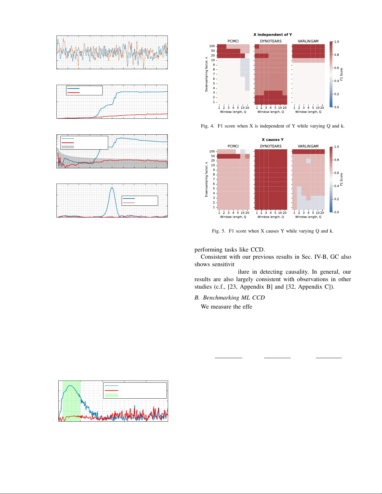
Rethinking Chronological Causal Disco v ery with Signal Processing Kurt Butler , Damian Machlanski, Panagiotis Dimitrakopoulos and Sotirios A. Tsaftaris School of Engineering, The Univ ersity of Edinbur gh, Edinbur gh, UK Causality in Healthcare AI Hub (CHAI), UK { kbutler2; d.machlanski; pdimitra; s.tsaftaris } @ed.ac.uk Abstract —Causal discovery pr oblems use a set of observ ations to deduce causality between variables in the real world, typically to answer questions about biological or physical systems. These observations ar e often recorded at r egular time intervals, deter - mined by a user or a machine, depending on the experiment design. There is generally no guarantee that the timing of these recordings matches the timing of the underlying biological or physical events. In this paper , we examine the sensitivity of causal discovery methods to this potential mismatch. W e consider empir - ical and theoretical evidence to understand how causal discovery performance is impacted by changes of sampling rate and window length. W e demonstrate that both classical and recent causal discovery methods exhibit sensitivity to these hyperparameters, and we discuss how ideas from signal processing may help us understand these phenomena. Index T erms —causal disco very , time series, sampling rate, graph topology inference, Nyquist rate I . I N T RO D U C T I O N Causal information is important because it allows us to reason about the world and the ef fects of how we interact with the world. In some cases, we may be uncertain of the presence or nature of causal relationships in real systems, and so we wish to infer the existence of causalities through data. One such task is causal discov ery , a detection-theoretic task in which one attempts to perform graph topology inference of a causal system [1]. Causal graphs aim to represent relationships that generalize when the system is interv ened upon, shocked, or otherwise externally manipulated [2]. In this work, our particular interest is in the chronological causal discovery (CCD) task, where the goal is to detect causal influences between signals or time series. The gold standard for modelling how natural systems e volve in time, and by extension their causal relationships, is dif- ferential equations [1]. Howe ver , instead of relying solely on continuous-time differential equations, we often in voke discrete-time models that abstract the underlying causal re- lationships [3]. Many recent works in the causal machine learning (causal ML) literature hav e focused on discrete-time models, without questioning how faithful these models are to the underlying continuous-time dynamics. If we consider the CCD task to be a problem of understanding the generati ve This work was supported by the UKRI AI programme and the Engineering and Physical Sciences Research Council, for CHAI - Causality in Healthcare AI Hub [grant number EP/Y028856/1]. process behind a data set, then the mismatch between discrete and continuous becomes clearly important. In this paper , we revisit the CCD task with a signal process- ing perspectiv e. W e outline a fe w fundamental concerns about modelling and detecting causal influences with time series, and demonstrate that those concerns apply to both classical and modern causal discov ery methods. Finally , we conclude with some reflections on what the signal processing community can offer to the pursuits of causality . I I . A P R I M E R O N C AU S A L D I S C OV E RY M E T H O D S Here we provide a high le vel re vie w of the chronological causal discovery task, and some representative approaches to the CCD task. Our list is necessarily non-e xhaustiv e, is intended to highlight a representative subset of methods, and we only consider approaches for stationary processes (Methods for non-stationary processes are beyond the scope of the current work). a) Granger Causality (GC) and T ransfer Entr opy (TE): While GC is potentially the oldest approach to detecting causal influences [4], it remains incredibly popular and is still activ ely discussed [5]. Although GC has been criticized as not representative of “true” causality , due to the possibility of unobserved confounding, the GC principle can be used as a part of “true” causal inference under certain assumptions [6, pp. 202-208]. The argument that unobserved confounding biases inference also applies to causal ML algorithms, which is why their assumptions often include some version of causal sufficienc y [7]. The classical GC algorithm fits linear autore- gressiv e models to the signals of interest and detects causality when conditioning on the putative cause improv es prediction. There are many other variants of GC that change the models being used, or the test statistic used to make a decision. T ransfer entropy (TE), a relati ve of the GC approach, formu- lates detection using information theory instead of predictiv e performance [8]. TE measures directed information flo w , al- lowing it to detect nonlinear influences that linear prediction models may miss. TE is argued to be more general than the standard GC approach, since the principles of information theory are innately model agnostic and nonlinear [9]. For Gaussian systems, TE and GC are ev en equiv alent [10]. Since TE is sometimes thought of as an extension of the GC test, TE depends on the sampling rate and window size in a similar manner to the GC test. b) Constraint-based: Constraint-based methods are a family of classical approaches to (static) causal discov ery that are based on conditional independence (CI) tests to recov er a graph skeleton, further refined with a set of constraining rules to orient edges. The Peter-Clark (PC) algorithm is a prime representativ e of such methods [11]. PC has been recently extended to temporal settings with momentary CI tests, in- troduced as PCMCI [12], which proved particularly robust to autocorrelated data, b ut limited to detecting lagged relation- ships. This limitation has been addressed with PCMCI+ that also handles instantaneous connections [13]. c) Functional-based: The lack of causal graph identifi- ability from observ ational data when using constraint-based methods has led to new approaches with stronger assumptions pertaining to the functional form of the data generating pro- cess, leading to identifiability guarantees. A foundational work in this category , [14], introduced identifiable models based on linearity and non-Gaussianity (LiNGAM). This core idea was later extended to time series with V ARLiNGAM [15]. Another notable work in functional models instead assumes additi ve noise models to obtain identifiability [16], which was later also applied to temporal problems as T iMINo [17]. d) Gradient-based: The challenging nature of learning causal graphs from data (i.e., discrete space) has been ad- dressed with NOTEARS [18] by casting the (acyclic) graph learning task into the continuous space, notably enabling the use of con ventional optimizers, such as stochastic gradient descent, in the graph inference task. This idea has been further extended to time series with D YNOTEARS [19] that simultaneously learns instantaneous and lagged relationships. e) Cr oss Mapping: Methods of this category assume that the observed time series were generated by a latent determin- istic dynamical systems, which is a class of problems that GC fails on [20]. V arious versions of T akens’ theorem assert that the latent state-space can be reconstructed from a bank of time- lagged filters under mild assumptions [21]. A cross mapping between these reconstructions is then interpreted as a signature of causal influence. Con vergent cross mapping (CCM), [20], is the most popular CCD method based on this logic. Like GC, other methods of this type use different test statistics to infer the existence of a cross map [22], [23]. Although the restrictiv e assumptions required for cross mapping methods may hinder their generality [24], cross mapping methods are good e xamples of CCD methods that are neither based on the GC principle nor causal ML algorithms. The methods GC, TE, and CCM originated from fields such as econometrics, neuroscience and climate science, with a specific focus on analysing time series, and are somewhat established within the signal processing literature. In contrast, methods such as PCMCI, D YNO TEARS, and V ARLiNGAM emerged from the causal ML literature, generalizing ap- proaches for causal discovery on static data to time series. Although dev eloped separately , signal processing and causal ML approaches to the CCD task are not unrelated. On the contrary , we argue that all of these approaches are related, and require similar considerations for hyperparameter selection. Win dow Gr ap h Summ ar y Gr ap h … … … … … … Y t - 1 X t - 1 Z t - 1 Y t - 2 X t - 2 Z t - 2 Y t X t Z t Y X Z Fig. 1. Descriptions of a causal system using a window graph and a summary graph, respectiv ely . A summary graph could be induced by a window graph by aggregating over the edges in a window graph. I I I . P R O B L E M F O R M U L A T I O N W e now introduce some basic notation, and then introduce the problem of temporal robustness of CCD algorithms. A. Notation Let x t = [ x 1 ,t , . . . , x D,t ] ⊤ ∈ R D denote a multi variate signal observed at discrete time t . T o frame the problem, we consider models of the following form. The CCD methods described in Sec. II do not necessarily use these models in their formulation, but it is helpful to specify a model to clarify the scope of our task. Let us assume a data generati ve process, x t = F ( x t − 1 , . . . , x t − Q , w t ) , (1) where F is a vector -valued function depending on pre vious values of the multi variate signal x t and an exogeneous noise variable, w t ∼ p ( w t ) . The parameter Q is kno wn as the window length , which measures the amount of memory (measured in discrete time) that the model has. W e imagine the discrete times to correspond to regular observations of a real-world physical process that is observed with sampling rate, f S . In some applications, changing f S is impossible because only data is recei ved and the modeller has no access to the recording instrument. Ho wev er, ev en in such cases, data may be record in a high-resolution format and then do wnsampled as a part of preprocessing. As such, we will also discuss the ef fect of modifying the sampling rate as a parameter . Modification of the sampling is often done by downsampling, where we define the downsampling factor , k = f orig inal S /f new S . Finally , it is sometimes more con venient to discuss sampling rate in terms of its reciprocal, the sampling period , denoted τ = 1 /f S . B. Chr onological Causal Discovery In the CCD task, we attempt to estimate the topology of a graph that is faithful to the data-generative process. Sev eral methods to perform the CCD task are mentioned in Sec. II. These methods can be separately into two categories depending on the type of graph that the y output, shown in Fig. 1. W indow graphs are directed graphs o ver a set of nodes x i,t , i = 1 , ..., D and their time lags x i,t − q for q = 1 , ..., Q . In comparison, a summary graph only has D nodes, corresponding to each time series x i,t . Edges in the window graph specify the time delay associated with a causal relationship, while the summary graph describes that there exists some causal relationship, in volving one or more time lags. For methods such as PCMCI, D YNO TEARS and V ARLiNGAM, a window graph is used to describe causal relationships. Meanwhile, the outputs of GC, TE, and CCM are better described as summary graphs. C. T emporal Rob ustness of CCD Methods One challenge of causal reasoning with statistical models is that there is an important distinction between the true data gen- erativ e process (DGP) and our model of that process. In other tasks, like prediction, classification, or generati ve modelling, this distinction is less important since those tasks only require that the model match the statistics of the DGP , regardless of how the model is implemented. In causal modelling, ho wever , we hav e less freedom in that we need the statistical model to more accurately mimic the DGP . a) A case study fr om neur oscience: In real systems, any flow of information comes with some time delay , as even light is not capable of instantaneous transportation. As such, if one wishes to detect a causal influence between two processes, then the modeller must cast the right net. For example, in [25], the task was to detect causal influence between two brain re gions. As the window length Q was v aried, the strength of causal influence, as estimated by the model, also v aried. The true time delay associated with the causal influence was hypothesized to be around 8 milliseconds, according to e xpert kno wledge. Because the sampling rate was τ = 1 millisecond, it is then expected that a model with windo w length near Q ≈ 8 would be appropriate to detect the ef fect. It was observed that for small values of Q , only a weak causal influence could be detected. Meanwhile, for Q ≫ 8 , the estimated causal strength was also weaker . For values near Q = 8 , there was a stronger casual strength observed. The takeaway from this study , for the current discussion, is that there is a limited range of values of Q for which causality can be detected. b) Effects of sampling rate: Crucially for the model (1) to be considered causal , we enforce F to only depend on past values of x t , and not future values. If we allo w F to also take x t as an input, we say that the model admits instantaneous effects [6, p.198]. Modelling instantaneous ef fects requires us to impose acyclicity assumptions on graphs produced by the model. Howe ver , instantaneous effects can often be considered as artifacts of a low sampling rate, f S (or a high sampling period τ ). Besides instantaneous ef fects, it has been found that subsampling in excess ( ↓ f S ) makes the performance of causal methods deteriorate [19], [26]–[28]. c) P arameter selection: Beyond the concerns of causal modelling, parameters such as Q are used in other models, and therefore there are e xisting methods for selecting their v alues. There is some temptation to assume that a Q = 1 is enough, but often times they cannot capture complex dynamics. This is somewhat obvious for (fully observed) linear systems, since their dynamics can be e xpressed using a single transition matrix and only one lag [29]. In general, Q > 1 is required to yield a good description of a system’ s dynamics. Preferences for how to select Q are often method dependent. A na ¨ ıve approach is to select a lar ge value for Q , since graphs corresponding to a smaller value of Q are typically contained within the same model class. Howe ver , this approach is not justified by an y principle, and extreme choices of Q may not yield good results, as we shown in Sec. IV -A. Akaike and Bayesian information criteria are popular metrics for V ARX models and their relati ves [30]. This When using methods like CCM, the method of false-nearest neighbors is often employed to select Q [31]. These methods vary significantly in their assumptions and their logic, but they share a common essence. Systems which are incompletely observed hav e additional degrees of freedom that cannot be modelled with just one lag, and so the additional lags are required to gain information about the dynamics and state of the unobserved system. I V . E X P E R I M E N TA L R E S U LT S : B E N C H M A R K I N G C C D M E T H O D S W e now examine the empirical evidence that proper se- lection of τ and Q matter for the CCD task. W e begin by benchmarking a few common CCD algorithms from the causal ML literature. W e then replicate similar phenomena using the methods of Granger causality . T aking Granger causality as a reference, we then discuss phenomena that appear in extreme choices of hyperparameter selection. In both experiments, a biv ariate system with two v ariables x and y is simulated. The signal x is generated as a smoothly varying stochastic process, and y is generated using a delay filter applied to x , with another autoregressi ve noise process added to the output. If x is considered to be signal, then the signal-to-noise ratio in y is 80-to-20. The linear filter is designed such that the time delay from input-to-output is about 50 samples in the base sampling rate. A. GC - V arying Q and k W e no w take a closer look at GC and its rob ustness to varying the hyperparameters. In Fig. 2, we visualize the per- formance of three different causality detectors vs the window length Q . W e employ two different GC tests, as well as a TE version. The variance-reduction version of GC detects causation x ⇒ y if 1 − V ar ( y t | x t − 1 , ..., x t − Q , y t − 1 , ..., y t − Q ) V ar ( y t | y t − 1 , ..., y t − Q ) > θ threshold , where v ariance is measured using the fit of a linear model. The decision threshold is selection by the user . Similarly , we also use an F -statistic version of the GC test that exploits that a ratio of v ariance estimators obeys an F -distrib ution. W e visualize the decision threshold for a 0.1 percent confidence. Finally , the TE estimator uses the Shannon entropy computed from the a binary binning approach. Similar results where ob- served for other numbers of bins, e.g. 5 bins. The approaches 0 100 200 300 400 500 600 700 800 900 1000 Time (samples) -10 -5 0 5 10 Signal value Raw data 0 10 20 30 40 50 60 70 80 90 100 Window length, Q, (in lags) 0 0.5 1 Variance reduction score Granger causality (Variance reduction score) x ) y (correct) x ( y (incorrect) 0 10 20 30 40 50 60 70 80 90 100 Window length, Q, (in lags) 10 0 10 2 F-statistic Granger causality (F-statistic) x ) y (correct) x ( y (incorrect) Rejection region (0.1%) 0 10 20 30 40 50 60 70 80 90 100 Window length, Q, (in lags) 0 0.1 0.2 0.3 Transfer entropy Discrete transfer entropy x ) y (correct) x ( y (incorrect) Fig. 2. V arying the window length Q. based on GC sho w that causality cannot reliably be detected when Q < 50 . TE was only able to detect causation when Q was matched to the propagation delay of the underlying causal signal. These findings are consistent with [28]. Similarly , in Fig. 3, we vary the sampling rate by downsam- pling. W e employ the v ariance-reduction GC detector with a window length Q = 5 . In green, we visualize an approximate detection windo w , which is the region in which the 50-lag propagation delay is contained between q = 1 and q = 5 lags after downsampling by k . As one might hope, this heuristic anticipates where the GC test has the best results. Ho wev er , the detection windo w cannot be computed without knowledge of the propagation delay of causal influence in the true system, which is information that is often not usually av ailable when 0 50 100 150 200 250 Downsampling factor, k 0 0.2 0.4 0.6 0.8 Variance reduction score Granger causality (Variance reduction score) x ) y (correct) x ( y (incorrect) Detection window (heuristic) Fig. 3. V arying the downsampling factor , k 1 2 3 4 5 10 20 W indow length, Q 100 50 20 10 9 8 7 6 5 4 3 2 1 Downsampling factor, k PCMCI 1 2 3 4 5 10 20 W indow length, Q D YNOTEARS 1 2 3 4 5 10 20 W indow length, Q V ARLiNGAM 0.0 0.2 0.4 0.6 0.8 1.0 F1 Scor e X independent of Y Fig. 4. F1 score when X is independent of Y while varying Q and k. 1 2 3 4 5 10 20 W indow length, Q 100 50 20 10 9 8 7 6 5 4 3 2 1 Downsampling factor, k PCMCI 1 2 3 4 5 10 20 W indow length, Q D YNOTEARS 1 2 3 4 5 10 20 W indow length, Q V ARLiNGAM 0.0 0.2 0.4 0.6 0.8 1.0 F1 Scor e X causes Y Fig. 5. F1 score when X causes Y while varying Q and k. performing tasks like CCD. Consistent with our previous results in Sec. IV -B, GC also shows sensitivity to both hyperparameters that can determine its success or failure in detecting causality . In general, our results are also lar gely consistent with observations in other studies (c.f., [23, Appendix B] and [32, Appendix C]). B. Benchmarking ML CCD W e measure the ef fecti veness of inferring the correct causal relationship between X and Y with F1 score. Below we define F1 using (R)ecall and (P)recision, which in turn tak e into account true positiv es (TPs), false negati ves (FNs) and false positiv es (FPs) obtained from comparing the true and predicted adjacency matrix encoding the causal graph. R = T P T P + F N , P = T P T P + F P , F1 = 2 × R × P R + P . Intuitiv ely , higher F1 is better and F1 =1 indicates perfectly recov ered graph. W e consider two settings wherein X either is independent of, or causes, Y , results of which are depicted in Fig. 4 and 5 respectively . From both cases it is clear that v arying hyperparameters Q and k has a large impact on the inferred causalities (i.e., colors change across Q and k). The right values for Q and k that lead to the right graph (dark red) also depend on used CCD algorithm, which is consistent with a similar observation from causal discovery on static data that hyperparameter rob ustness can be algorithm-specific [33]. V . D I S C U S S I O N Discussions of sampling rate selection often consider the Nyquist-Shannon theorem to produce lower -bounds on sam- pling rates that allow for lossless signal reconstruction [34]. In a similar spirit, a causal Nyquist theorem would consider the spectral properties of a causal mechanism, and provide a lower -bound on the sampling rate required for correct causal inference. One approach, assuming we model causation via linear time-inv ariant filters, is to study transfer functions [35]. Nyquist theorems typically assume that frequency spectra are band-limited. If the transfer function of a linear filter is band- limited, then one could define a Nyquist threshold for sampling rates, which would upper-bound the Nyquist rate of any signal output by the filter . Howe ver , not all linear filters are band- limited; notably , high-pass filters hav e the complete opposite behaviour . In such cases, it is unclear how one might define a Nyquist rate. Furthermore, although sub-Nyquist sampling can introduce artifacts, it may be possible that CCD performance is not adversely affected. It remains to be seen if a good notion of a causal Nyquist rate can be defined. V I . C O N C L U S I O N Our observ ations point to challenges that CCD methods face when applied to real data. These challenges apply to both traditional and modern methods alike. These challenges were also observed despite our limited problem scope, ignoring complexities that arise from nonstationarity , latent confounder processes, and multiple time scales. The signal processing community has clear opportunities to contribute to the ov er- coming these challenges and dev eloping better CCD methods. V I I . A C K N OW L E D G E M E N T W e thank several individuals for useful discussions: Emily Stephen, Urbashi Mitra, Michael Camilleri, and Petar Djuri ´ c. R E F E R E N C E S [1] B. Sch ¨ olkopf, F . Locatello, S. Bauer, N. R. Ke, N. Kalchbrenner, A. Goyal, and Y . Bengio, “T oward causal representation learning, ” Pr oceedings of the IEEE , vol. 109, no. 5, pp. 612–634, 2021. [2] J. Pearl, Causality . Cambridge University Press, 2009. [3] S. Beckers, F . Eberhardt, and J. Y . Halpern, “ Approximate causal abstractions, ” in Uncertainty in Artificial Intelligence , pp. 606–615, PMLR, 2020. [4] C. W . Granger, “Investig ating causal relations by econometric models and cross-spectral methods, ” Econometrica: Journal of the Econometric Society , pp. 424–438, 1969. [5] A. Shojaie and E. B. Fox, “Granger causality: A revie w and recent advances, ” Annual Review of Statistics and Its Application , vol. 9, no. 1, pp. 289–319, 2022. [6] J. Peters, D. Janzing, and B. Sch ¨ olkopf, Elements of Causal Infer ence: F oundations and Learning Algorithms . The MIT Press, 2017. [7] S. Beckers, “Causal sufficiency and actual causation, ” J ournal of Philo- sophical Logic , vol. 50, no. 6, pp. 1341–1374, 2021. [8] T . Schreiber , “Measuring information transfer , ” Physical Review Letters , vol. 85, no. 2, p. 461, 2000. [9] R. V icente, M. Wibral, M. Lindner, and G. Pipa, “Transfer entropy—a model-free measure of effecti ve connectivity for the neurosciences, ” Journal of Computational Neuroscience , vol. 30, no. 1, pp. 45–67, 2011. [10] L. Barnett, A. B. Barrett, and A. K. Seth, “Granger causality and transfer entropy are equiv alent for Gaussian variables, ” Physical Review Letters , vol. 103, no. 23, p. 238701, 2009. [11] P . Spirtes, C. N. Glymour, and R. Scheines, Causation, prediction, and sear ch . MIT Press, 2000. [12] J. Runge, P . Now ack, M. Kretschmer, S. Flaxman, and D. Sejdinovic, “Detecting and quantifying causal associations in large nonlinear time series datasets, ” Science Advances , vol. 5, no. 11, p. eaau4996, 2019. [13] J. Runge, “Discov ering contemporaneous and lagged causal relations in autocorrelated nonlinear time series datasets, ” in Conference on uncertainty in artificial intelligence , pp. 1388–1397, PMLR, 2020. [14] S. Shimizu, P . O. Hoyer , A. Hyv ¨ arinen, A. Kerminen, and M. Jordan, “ A linear non-gaussian acyclic model for causal discovery ., ” Journal of Machine Learning Resear ch , vol. 7, no. 10, 2006. [15] A. Hyv ¨ arinen, K. Zhang, S. Shimizu, and P . O. Hoyer , “Estimation of a structural vector autoregression model using non-gaussianity ., ” Journal of Machine Learning Research , vol. 11, no. 5, 2010. [16] P . Hoyer, D. Janzing, J. M. Mooij, J. Peters, and B. Sch ¨ olkopf, “Nonlinear causal discovery with additive noise models, ” Advances in Neural Information Pr ocessing Systems , vol. 21, 2008. [17] J. Peters, D. Janzing, and B. Sch ¨ olkopf, “Causal inference on time series using restricted structural equation models, ” Advances in Neural Information Processing Systems , vol. 26, 2013. [18] X. Zheng, B. Aragam, P . K. Ravikumar , and E. P . Xing, “D AGs with no tears: Continuous optimization for structure learning, ” Advances in Neural Information Pr ocessing Systems , vol. 31, 2018. [19] R. Pamfil, N. Sriwattanaworachai, S. Desai, P . Pilgerstorfer , K. Geor- gatzis, P . Beaumont, and B. Aragam, “Dynotears: Structure learning from time-series data, ” in International Conference on Artificial Intelli- gence and Statistics , pp. 1595–1605, PMLR, 2020. [20] G. Sugihara, R. May , H. Y e, C.-h. Hsieh, E. De yle, M. Fogarty , and S. Munch, “Detecting causality in complex ecosystems, ” Science , vol. 338, no. 6106, pp. 496–500, 2012. [21] T . Sauer , J. A. Y orke, and M. Casdagli, “Embedology , ” Journal of Statistical Physics , vol. 65, no. 3, pp. 579–616, 1991. [22] Z. Benk ˝ o, ´ A. Zlatniczki, M. Stippinger, D. Fab ´ o, A. S ´ olyom, L. Er ˝ oss, A. T elcs, and Z. Somogyv ´ ari, “Bayesian inference of causal relations between dynamical systems, ” Chaos, Solitons & F ractals , vol. 185, p. 115142, 2024. [23] K. Butler, D. W axman, and P . Djuric, “T angent space causal inference: Lev eraging vector fields for causal discovery in dynamical systems, ” Ad- vances in Neural Information Pr ocessing Systems , vol. 37, pp. 120078– 120102, 2024. [24] K. Butler , G. Feng, and P . M. Djuri ´ c, “On causal discovery with con vergent cross mapping, ” IEEE Tr ansactions on Signal Pr ocessing , vol. 71, pp. 2595–2607, 2023. [25] K. Butler , D. Cleveland, C. B. Mikell, S. Mofakham, Y . B. Saalmann, and P . M. Djuri ´ c, “ An approach to learning the hierarchical organization of the frontal lobe, ” in 2023 31st Eur opean Signal Pr ocessing Confer- ence (EUSIPCO) , pp. 1410–1414, IEEE, 2023. [26] J. Munoz-Benıtez and L. E. Sucar, “Synthetic time series: A dataset for causal discovery , ” 2023. [27] D. Danks and S. Plis, “Learning causal structure from undersampled time series, ” 2013. [28] L. Barnett and A. K. Seth, “Detectability of granger causality for subsampled continuous-time neurophysiological processes, ” Journal of Neur oscience Methods , vol. 275, pp. 93–121, 2017. [29] R. E. Kalman, “Mathematical description of linear dynamical systems, ” Journal of the Society for Industrial and Applied Mathematics, Series A: Control , vol. 1, no. 2, pp. 152–192, 1963. [30] P . Stoica and Y . Selen, “Model-order selection: a re view of information criterion rules, ” IEEE Signal Pr ocessing Magazine , vol. 21, no. 4, pp. 36–47, 2004. [31] M. B. Kennel, R. Bro wn, and H. D. Abarbanel, “Determining embedding dimension for phase-space reconstruction using a geometrical construc- tion, ” Physical Review A , vol. 45, no. 6, p. 3403, 1992. [32] P . P . Sanchez, D. Machlanski, S. McDonagh, and S. A. Tsaftaris, “Causal ordering for structure learning from time series, ” arXiv preprint arXiv:2510.24639 , 2025. Accepted for publication in TMLR. [33] D. Machlanski, S. Samothrakis, and P . S. Clarke, “Robustness of algorithms for causal structure learning to hyperparameter choice, ” in Causal Learning and Reasoning , pp. 703–739, PMLR, 2024. [34] Z. Zeng, J. Liu, and Y . Y uan, “ A generalized Nyquist-Shannon sampling theorem using the Koopman operator , ” IEEE T ransactions on Signal Pr ocessing , 2024. [35] N. Jalili and N. W . Candelino, “System transfer function analysis, ” in Dynamic Systems and Contr ol Engineering , p. 312–374, Cambridge Univ ersity Press, 2023.