A Stochastic Tube-Based MPC Framework with Hard Input Constraints

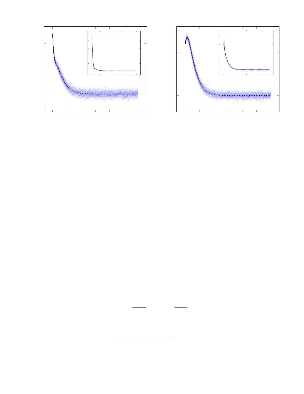
A Stochastic T ube-Based MPC F rame work with Hard Input Constraints Carlo Karam, Matteo T acchi-B ´ enard, and Mirko Fiacchini Abstract This work presents a stochastic tube-based model predictive control fr amew ork that guarantees hard input constr aint satisf action f or linear systems subject to unbounded additive disturbances . The approach relies on a structured design of probabilistic reachable sets that e xplicitly incor porates actuator saturation into the error dynamics and bounds the resulting nonlinearity within a conv e x embedding. The proposed con- troller retains the computational efficiency and structural advantages of stochastic tube-based approaches while ensuring state chance constraint satisfaction alongside hard input limits . Recursiv e feasibility and mean-square stability are estab lished f or our scheme , and a numerical e xample illustrates its eff ectiveness . Index T erms Predictive Control, Stochastic Optimal Control, Stochastic Model Predictive Control, Chance Constraints, Saturating Actuators I . I N T R O D U C T I O N Model Predictiv e Control (MPC) has established itself as a reliable framew ork for the optimal control of constrained dynamical systems and is widely adopted in applications where performance must be achiev ed subject to state and input limitations. In the presence of uncertainty , Robust MPC (RMPC) extends the nominal formulation by guaranteeing recursiv e feasibility and constraint satisfaction for all admissible disturbance realizations through a worst-case formulation, most notably through the tube-based approach [1]–[3]. Although such formulations provide strong deterministic guarantees, they typically induce conserv atism by shrinking the admissible state and input sets, thereby limiting achie v able performance [4]. Stochastic MPC (SMPC) has emerged as an alternati ve formulation that exploits probabilistic descriptions of disturbances [5]. By incorporating distributional information, SMPC often replaces hard constraint satisfaction with chance constraints, allowing for rare violations with user-prescribed probability levels. This relaxation generally enlarges the admissible region and improv es closed-loop performance compared to worst-case designs. Moreover , the stochastic framew ork enables the treatment of disturbances without kno wn bounded support [5], such as Gaussian noise, for which deterministic robust formulations are inherently inapplicable. Despite the substantial progress achiev ed in SMPC design, the treatment of input constraints remains an open problem. In contrast to state constraints, which can be meaningfully relaxed in a probabilistic sense, input constraints must be satisfied deterministically at all times as they often correspond to physical actuator saturation limits. Ensuring such guarantees in the presence of unbounded disturbances is nontrivial, as the stochastic feedback component may generate arbitrarily large control actions. Scenario and sample-based SMPC approaches can, in principle, accommodate state chance constraints together with hard input bounds by enforcing constraints ov er a suf ficiently large set of disturbance realizations [6]. Howe ver , these methods require access to disturbance samples, may entail significant computational effort, and typically pro vide guarantees only with respect to the sampled scenarios, without establishing strong closed-loop properties [5]. Analytical approaches instead rely on distributional or moment information of the disturbance. A prominent class of methods is based on affine disturbance-feedback parameterizations of the control la w , initially introduced for RMPC in [7] and adapted for chance-constrained systems in [8]. Such parameterizations enable con ve x reformulations of the stochastic optimal control problem This work has been submitted to the IEEE for possib le publication. The final pu blished v ersion may not be pub licly accessib le. Matteo T acchi-B ´ enard’ s work is suppor ted by the F rench National Research Agency (ANR) under the PIV OINE project grant ANR-25-CE48-1599-01. The authors are with Univ . Grenoble Alpes, Grenoble INP , CNRS, GIPSA-lab (e-mail: car lo .karam [at] gipsa-lab [dot] fr; matteo .tacchi [at] gipsa-lab [dot] fr; mir ko .fiacchini [at] gipsa-lab [dot] fr). 1 by optimizing jointly over open-loop inputs and feedback gains [5]. T o address hard input constraints under unbounded noise, [9], [10] introduced saturation within the affine parametrization, thereby ensuring deterministic input feasibility in the absence of state constraints; this frame work was subsequently extended to output-feedback settings in [11]. More recently , [12] generalized the approach to handle hard input bounds together with joint state constraints. While effecti ve, these formulations are often computationally demanding and do not scale ef ficiently with increasing prediction horizon or system dimension, as the number of decision v ariables gro ws accordingly . Stochastic tube-based approaches offer a structurally dif ferent alternati ve. Inspired by rob ust tube MPC, they decouple nominal trajectory optimization from uncertainty propagation by computing probabilistic reachable sets (PRS) offline and tightening constraints accordingly , resulting in a deterministic and lo w-dimensional MPC problem online [5]. Despite being extensi vely in vestigated as in [13]–[17], most existing stochastic tube schemes do not guarantee hard input constraints when disturbances are unbounded, as the ancillary feedback gain is fixed offline and may generate arbitrarily large inputs. Existing attempts to enforce deterministic actuator limits without assuming kno wn robust disturbance bounds ( [18], [19]) remain limited. In particular , output-feedback-based methods such as [20], [21] ensure that the applied input satisfies the constraints deterministically , but compromise recursiv e feasibility due to unrealistic input trajectories, only ensuring feasibility with a user-specified probability . More recently , a constraint- tightening SMPC framew ork for general nonlinear systems accommodating hard input constraints was proposed in [22], though its application to linear systems is not fully detailed and may introduce significant conserv atism. Moti vated by the abov e considerations, this work de velops a stochastic tube-based SMPC framework for linear systems that guarantees hard input constraint satisfaction under unbounded disturbances by explicitly incorporating actuator saturation into the system dynamics. Although this modeling choice introduces a nonlinearity in the error dynamics, we embed it within an ellipsoidal PRS construction. This enables the retention of linear nominal dynamics and ancillary feedback while ensuring deterministic satisf action of input constraints together with state chance constraint guarantees. The preliminary PRS design underlying the proposed framew ork can be found in [23]. In that work, we dev eloped a constructive method for computing ellipsoidal PRS for saturated linear systems subject to unbounded additiv e disturbances, based on con ve x bounds of the saturated error dynamics and an ensuing contraction analysis. The present work builds upon that foundation and makes the following contributions: 1) Integration into a complete SMPC scheme: we embed the PRS construction of [23] into a stochastic tube- based predicti ve control frame work with hard input constraints, yielding a tractable scheme that we term Saturation-A ware SMPC (SA-SMPC). 2) For the resulting SA-SMPC controller, we establish recursi ve feasibility and state chance constraint satisfaction under unbounded disturbances with known second moments. In addition, we provide rigorous closed-loop guarantees, including mean-square boundedness, both for the practically implemented nominal-cost formulation and for the ideal nonlinear formulation. The proposed framew ork guarantees the standard closed-loop properties typically required for SMPC schemes with hard input constraints, while explicitly accounting for the closed-loop structure of the error under the pre- stabilizing feedback in the offline constraint-tightening design. This enables a less conserv ativ e enforcement of hard input constraints than that provided in [22], where the tightening is ef fecti vely based on open-loop error predictions. T o the best of our kno wledge, no such framework exists. The remainder of this paper is organized as follows. Section II introduces the problem formulation and standing assumptions. Section III presents the con ve x PRS synthesis for the saturated error dynamics and details the conditions under which the base bound can be refined to reduce conserv atism. Section IV dev elops the full SA-SMPC scheme and establishes recursi ve feasibility , chance constraint satisfaction, and closed-loop stability properties. Finally , Section V provides numerical results validating the theoretical developments and compares the proposed method with a nominal MPC scheme as well as with the affine disturbance-feedback approach with hard input constraints of [12]. Lengthy technical proofs are deferred to Appendices I and II for completeness and clarity of exposition. A. Notation The set of positiv e integers is denoted by N and the set of nonnegativ e integers by N 0 . For integers a, b ∈ N with a ≤ b , we define N b a := { n ∈ N : a ≤ n ≤ b } . For a matrix A ∈ R n × m , the notation A ( j ) ∈ R n denotes its j -th column, while A j ∈ R m denotes its j -th row . For symmetric matrix A ∈ R n × m , Λ max ( A ) is the maximum eigen v alue of A . For P ≻ 0 and r > 0 , we define the ellipsoid E ( P , r ) := { e ∈ R n : e ⊤ P e ≤ r } . The Pontryagin 2 dif ference of two sets S , T ⊆ R n is defined as S ⊖ T := { s ∈ S | s + t ∈ S , ∀ t ∈ T } . For a matrix K ∈ R m × n and a set S ⊆ R n , we denote the image of S under the linear map K by K S := { K s ∈ R m | s ∈ S } . Finally , the measured state at time k is denoted x k , and the i -step-ahead state prediction made at time k is denoted x i | k , with x 0 | k = x k . 3 I I . P RO B L E M F O R M U L ATI O N Consider an uncertain linear time-in variant (L TI) system whose discrete-time dynamics obey x k +1 = Ax k + B u k + w k , (1) where x k ∈ R n , u k ∈ R m , and w k ∈ R n represent the system state, control input, and unkno wn process noise, respecti vely . The matrices A ∈ R n × n and B ∈ R n × m are fully kno wn. Assumption 1 (Noise distrib ution): The disturbance w k is independently and identically distributed (i.i.d.) according to an unknown distribution with zero mean and known variance, i.e. E [ w k ] = 0 , E h w ⊤ k w k i = W ≻ 0 for all k ∈ N 0 . Note that these conditions may be met by disturbance distributions with infinite support. The state constraint set X ⊆ R n and the input constraint set U ⊆ R m are defined as X : = { x ∈ R n | H x ≤ h } , U : = { u ∈ R m | ∥ u ∥ ∞ ≤ 1 } , W e impose state chance constraints, with user-defined violation probability ε ∈ (0 , 1) , as Pr { x k ∈ X | x 0 } ≥ 1 − ε, ∀ k ∈ N , (2) where the probability is conditioned on the initial state x 0 , and hard input constraints u k ∈ U , ∀ k ∈ N . (3) As usual in the SMPC framew ork, the aim is to solve an optimization problem at ev ery step k , minimizing over a sequence of i -steps ahead predicted states x i | k and inputs u i | k which relate to each other by x i +1 | k = Ax i | k + B u i | k + w i + k , x 0 | k = x k , (4) where the realized state x k is measurable. W e introduce the finite-horizon cost J N ( x k , u k ) : = E " N − 1 X i =0 ℓ ( x i | k , u i | k ) + V f ( x N | k ) # (5) to be minimized at time-step k , giv en a user-defined stage cost ℓ ( · , · ) , terminal cost V f ( · ) , and some horizon N ∈ N . The resulting finite-horizon stochastic optimal control problem can be thus stated as min x k , u k J N ( x k , u k ) , (6a) s . t . x i +1 | k = Ax i | k + B u i | k + w i + k , (6b) x 0 | k = x k , (6c) u i | k ∈ U , i ∈ N N 0 , (6d) Pr  x i | k ∈ X | x k  ≥ 1 − ε, i ∈ N N − 1 0 , (6e) Pr  x N | k ∈ X f | x k  ≥ 1 − ε, (6f) where x k = ( x i | k ) N i =0 , u k = ( u i | k ) N i =0 , and X f is an appropriately designed terminal constraint set. The optimization problem above is generally intractable due to the noncon ve xity and implicit nature of the chance constraints, which require e v aluating multiv ariate probability distributions ov er future uncertain states. T o obtain a tractable formulation, the problem is approximated through a constraint-tightening approach based on reachable sets, which ensures probabilistic feasibility while enabling online optimization of control inputs within the admissible set U . T o this end, we adopt a standard stochastic tube approach inspired by robust MPC schemes [1], splitting the predicted state into nominal and stochastic components x i | k = z i | k + e i | k , (7) 4 where z i | k denotes the nominal state, and e i | k represents its de viation with respect to the stochastic predicted state. The control input is parameterized as u i | k = v i | k + K e i | k . (8) where v i | k is the nominal input sequence optimized online (at every step k ), and K is a fixed stabilizing feedback gain computed of fline. Because the process noise may be unbounded (see Assumption 1), the error term e i | k may become arbitrarily large. Since K is fixed, this consequently makes it difficult to bound the beha vior of the pre-stabilizing control action K e i | k , and in turn ensure hard constraints u i | k ∈ U for all k ∈ N . T o address this issue, we incorporate the input constraints (3) directly into the system dynamics by introducing a saturation on the control input. The predicted state no w ev olves according to, x i +1 | k = Ax i | k + B φ  u i | k  + w i + k , (9) where φ : R m → R m is the element-wise saturation function φ j ([ u i | k ]) = sign  [ u i | k ] j  min    [ u i | k ] j   , 1  , (10) for all j ∈ N m 1 , with saturation bounds normalized to 1. For compactness, define f ( e i | k , v i | k ) : = Ae i | k + B  φ ( K e i | k + v i | k ) − v i | k  , (11) yielding the nominal and error dynamics z i +1 | k = Az i | k + B v i | k , (12a) e i +1 | k = f ( e i | k , v i | k ) + w i + k . (12b) Note that, if z 0 | k = x k then e 0 | k = 0 , from (7). For our de velopment, we require the following regularity conditions. Assumption 2 (Regularity conditions): (a) The matrix A is Schur stable. (b) ∥ v i | k ∥ ∞ ≤ 1 , for all i , k ∈ N 0 . Condition b) is imposed in the eventual SMPC scheme, and is equiv alent to enforcing (3) on the nominal system (gi ven normalized saturation bounds). The error dynamics in (12b) provide the basis for recasting the chance constraints into deterministic, tightened constraints on the nominal state vector . This process is detailed in the following section. I I I . P R O B A B I L I S T I C R E A C H A B L E S E T C O N S T RU C T I O N This section details the methodology used to construct the sets required to make the probabilistic constraints in (6e) and (6f) tractable. W e begin by formalizing the core set-theoretic concepts employed in that analysis. Definition 1 (Probabilistic Reachable Set): For a gi ven k ∈ N , a set R ε k is a horizon k Probabilistic Reachable Set (PRS) with violation probability ε ∈ [0 , 1] for a stochastic process { e i } i ∈ N ∈ R n if Pr { e k ∈ R ε k | e 0 = 0 } ≥ 1 − ε. Definition 2 (Probabilistic Ultimate Bound, [24]): A set R ε is a Probabilistic Ultimate Bound (PUB) with violation probability ε ∈ [0 , 1] for a stochastic process { e k } k ∈ N ∈ R n if, for any initial condition e 0 , there exists a finite time t ( e 0 ) such that Pr { e k ∈ R ε } ≥ 1 − ε, ∀ k ≥ t ( e 0 ) . While the preceding definitions are valid for sets of arbitrary geometry , the subsequent dev elopment focuses on their ellipsoidal representations. Specifically , we de velop a recursi ve procedure to compute ellipsoidal PRS for the i -step ahead predicted error e i | k conditioned on e 0 | k = 0 . 5 A. Conv ex Bounds of Saturated Functions Reachability analysis typically relies on set propagation methods that require explicit knowledge of the system’ s dynamics to compute reachable sets under certain fav orable conditions [25], [26]. Such conditions break down for the nonlinear error dynamics given abov e due to the hard nonlinearity introduced by the saturation function φ ( · ) and the dependence on the nominal input v . As a result, standard recursi ve set computation techniques are hardly applicable. T o address this issue, we aim to bound f ( e i | k , v i | k ) within a well-defined con ve x set (as in [27]), which allo ws for the computation of outer approximations of the true reachable sets of the error dynamics. Definition 3 (Support Function): For a nonempty conv ex set C ⊆ R n , the support function ev aluated at η ∈ R n is defined as δ C ( η ) = sup x ∈ C η ⊤ x . The properties inherent to support functions lead to the following set inclusion theorem. Theorem 1 ( [28]): F or nonempty , con ve x, and closed sets C 1 and C 2 , the inclusion C 1 ⊆ C 2 holds if and only if δ C 1 ( η ) ≤ δ C 2 ( η ) for every η ∈ R n . From this result, we present the subsequent theorem, v alid for any e ∈ R n . Theorem 2: F or any v satisfying ∥ v ∥ ∞ ≤ 1 , the function f ( e, v ) = Ae + B ( φ ( K e + v ) − v ) is contained within the set F ( e ) , wher e F ( e ) = co        A + X j ∈ J B ( j ) K j  e    J ⊆ N m 1    . (13) Pr oof: Consider first the scalar case m = 1 and assume K e ≥ 0 . Gi ven the constraint − 1 ≤ v ≤ 1 , it follo ws that − 1 ≤ K e + v ≤ 1 + K e , and consequently φ ( K e + v ) = ( K e + v for K e + v ≤ 1 , 1 for K e + v ≥ 1 . This leads to φ ( K e + v ) − v = ( K e for K e + v ≤ 1 , 1 − v for K e + v ≥ 1 . Since K e is unbounded abov e and 1 − v ≥ 0 , the inequality 0 ≤ φ ( K e + v ) − v ≤ K e holds. A similar argument for K e < 0 yields K e ≤ φ ( K e + v ) − v ≤ 0 . Generalizing to arbitrary m , for any index subset J ⊆ N m 1 and j ∈ J , we obtain ( 0 ≤ φ ( K j e + v j ) − v j ≤ K j e when K j e ≥ 0 , K j e ≤ φ ( K j e + v j ) − v j ≤ 0 when K j e < 0 . By lev eraging the support function, we deduce that for e very η ∈ R n and ev ery j ∈ J , η ⊤ B ( j ) ( φ ( K j e + v j ) − v j ) ∈ co n 0 , η ⊤ B ( j ) K j e o ⊆ R . Equi valently , the bounds min n 0 , η ⊤ B ( j ) K j e o ≤ η ⊤ B ( j ) ( φ ( K j e + v j ) − v j ) ≤ max n 0 , η ⊤ B ( j ) K j e o , are satisfied. Therefore, for any η ∈ R n , any v with ∥ v ∥ ∞ ≤ 1 , and any e ∈ R n , there exists an inde x set J ( e, η ) ⊆ N m 1 such that η ⊤ f ( e, v ) = η ⊤ Ae + X j ∈ N m 1 η ⊤ B ( j ) ( φ ( K j e + v j ) − v j ) ≤ η ⊤ Ae + X j ∈ J ( e,η ) η ⊤ B ( j ) ( φ ( K j e + v j ) − v j ) . Application of Theorem 1 confirms that f ( e, v ) ∈ F ( e ) . Theorem 2 establishes that for ev ery e ∈ R n and ev ery ∥ v ∥ ∞ ≤ 1 , the v alue f ( e, v ) lies within the polytope F ( e ) , whose vertices correspond to the linear combinations  A + P j ∈ J B ( j ) K j  e for all J ⊆ N m 1 . These vertices correspond to realizations of dif ferent saturation scenarios: full, partial, and no saturation [29]. 6 The following corollaries are direct consequences of Theorem 2, deri ved via con ve xity arguments. T o simplify notation, for e very J ⊆ N m 1 define A K ( J ) =  A + P j ∈ J B ( j ) K j  . Corollary 1: If Assumption 2 is satisfied, then the inequality f ( e, v ) ⊤ P f ( e, v ) ≤ max J ⊆ N m 1 e ⊤ A K ( J ) ⊤ P A K ( J ) e, (14) holds for every e ∈ R n . Pr oof: This assertion follo ws directly from Theorem 2, by con ve xity of R n ∋ f 7− → f ⊤ P f . These results indicate that the nonlinear dynamics f ( e, v ) are bounded by the behavior of the linear systems A K ( J ) e for all subsets J ⊆ N m 1 and all admissible v . Consequently , bounds deriv ed for A K ( J ) e are also v alid for the saturated system. B. Base PRS Synthesis Utilizing the results from Section III-A, we now construct a PRS for the error state e i | k ∈ R n . Proposition 1: Let Assumptions 1 and 2 hold, and consider a symmetric positive definite matrix P = P ⊤ ≻ 0 that satisfies A K ( J ) ⊤ P A K ( J ) ⪯ λP , ∀ J ⊆ N m 1 (15) for some contraction rate λ ∈ [0 , 1) . Then, for all i, k ∈ N , the bound E h e ⊤ i +1 | k P e i +1 | k i ≤ λ E h e ⊤ i | k P e i | k i + T r ( P W ) (16) holds for system (12b) and E h e ⊤ i | k P e i | k i ≤ 1 − λ i 1 − λ T r( P W ) , (17) if e 0 | k = 0 . Pr oof: If (15) is satisfied, Corollary 1 can be applied, yielding f ( e i | k , v i | k ) ⊤ P f ( e i | k , v i | k ) ≤ λe ⊤ i | k P e i | k . for all e i | k ∈ R n . This inequality and Assumption 1 lead to the following relationship: E [( f ( e i | k , v i | k ) + w i + k ) ⊤ P  f ( e i | k , v i | k ) + w i + k  ] = E h f ( e i | k , v i | k ) ⊤ P f ( e i | k , v i | k ) i + E h w ⊤ i + k P w i + k i = E h f ( e i | k , v i | k ) ⊤ P f ( e i | k , v i | k ) i + T r ( P W ) ≤ λ E h e ⊤ i | k P e i | k i + T r ( P W ) . Considering the error dynamics (12b), we obtain (16). The remainder of the proof proceeds by induction. For i = 0 , E h e ⊤ 0 | k P e 0 | k i = 0 by assumption. For i = 1 , E h e ⊤ 1 | k P e 1 | k i ≤ λ E h e ⊤ 0 | k P e 0 | k i + T r( P W ) ≤ T r( P W ) . For i = t , one gets E h e ⊤ t | k P e t | k i ≤ λ E h e ⊤ t − 1 | k P e t − 1 | k i + T r( P W ) ≤ t − 1 X j =0 λ j T r( P W ) . The sequence of upper bounds for E h e ⊤ i | k P e i | k i forms a geometric series with ratio λ . Thus, inequality (17) is v alid for any contraction rate 0 ≤ λ < 1 . Remark 1: In the preceding proof, Assumption 1 was used to nullify the cross-terms. Should the analysis be ex- tended to incorporate biased or correlated disturbances, the terms E [ w i + k ] ⊤ P E [ w i + k ] and E h f  e i | k , v i | k  ⊤ P w i + k i would need to be introduced, respectively . Accommodating such terms within the present framew ork is possible by assuming known bounds on the means and cov ariance matrices, and following the approach detailed in [30]. Combining the pre vious result with Markov’ s inequality yields the follo wing lemma. 7 Lemma 1: The sequence of sets defined by R ε i ( λ ) =  e ∈ R n     e ⊤ P e ≤ 1 − λ i ε (1 − λ ) T r ( P W )  , (18) forms a sequence of Marko v-based ellipsoidal PRS for violation pr obability ε . Pr oof: Applying Markov’ s inequality to the random variable e ⊤ k P e i | k gi ves Pr n e ⊤ i | k P e i | k ≥ r o ≤ E h e ⊤ i | k P e i | k i r . Plugging in the bound in (17) into the right hand side yields for r = 1 − λ i ε (1 − λ ) T r( P W ) Pr n e ⊤ i | k P e i | k ≤ r o ≥ 1 − 1 − λ i r (1 − λ ) T r( P W ) = 1 − ε. T aking the limit of the Marko v-based PRS R ε i ( λ ) as i → ∞ produces the following Markov-based ellipsoidal PUB set. Lemma 2: The set defined by R ε ( λ ) =  e ∈ R n     e ⊤ P e ≤ 1 ε (1 − λ ) T r ( P W ) + ζ  , (19) with ζ > 0 , is a Marko v-based ellipsoidal PUB for violation pr obability ε . Pr oof: For any initial condition e 0 | k ∈ R n , the recursion in (16) implies lim i →∞ E h e ⊤ i | k P e i | k i ≤ lim i →∞  λ i E h e ⊤ 0 | k P e 0 | k i + 1 − λ i 1 − λ T r( P W )  = 1 1 − λ T r ( P W ) . Hence, by definition of limits, for e very ε, ζ > 0 and ev ery e 0 | k ∈ R n , there exists t ( e 0 | k ) ∈ N such that E h e ⊤ i | k P e i | k i ≤ 1 1 − λ T r( P W ) + εζ , ∀ i ≥ t ( e 0 | k ) . Applying Markov’ s inequality yields Pr  e ⊤ i | k P e i | k ≤ 1 ε  1 1 − λ T r( P W ) + εζ  ≥ 1 − ε, ∀ i ≥ t ( e 0 | k ) , which proves the result. Note that for any stabilizing gain K , condition (15) also requires that the quadratic function satisfies the L yapuno v condition with the same rate λ i.e. A ⊤ P A ⪯ λP . (20) The resulting contraction rate λ therefore characterizes the open-loop or fully saturated dynamics. This bound, equi valent to the one in [22] for a linearized system, is inherently conserv ativ e, as it ignores the stronger contraction achie vable near the origin under non-saturated, closed-loop operation. The following section introduces a refined bound to address this limitation. C . Conditional Refinement of Base PRS The Markov-based PRS and PUB presented in Lemmas 1 and 2 exhibit conservatism, as they rely on a contraction rate λ that does not fully characterize the system dynamics. In practice, the system often ev olves in a region where the control input K e + v does not saturate, and the dynamics are linear . This region is defined below . Definition 4 (Saturation Region of Linearity [31]): The region of linearity for system (12b), denoted R L , is the set of all error states e for which φ ( K e + v ) = K e + v . Inside R L , the predicted error dynamics reduce to e i +1 | k = ( A + B K ) e i | k + w i + k . The following corollary , which follows from Theorem 2, Proposition 1, and the preceding definition, is presented. 8 Corollary 2: Let Assumptions 1 and 2 hold and P = P ⊤ ≻ 0 be a matrix satisfying the L yapunov inequality (15) with contraction rate λ ∈ [0 , 1) . Suppose the gain K ∈ R n × m and a scalar λ L ∈ R satisfy λ L ≤ λ, (21a) ( A + B K ) ⊤ P ( A + B K ) ⪯ λ L P , (21b) Then, the inequality E h e ⊤ k +1 P e k +1 i ≤ λ L E h e ⊤ k P e k i + T r( P W ) , (22) holds for every k ∈ N 0 such that e k ∈ R L . Pr oof: Condition (21b) establishes that the contraction rate λ L , applicable within R L , is less than or equal to λ . Thus e ⊤ i | k P e i | k = E  e ⊤ k P e k  for all e i | k ∈ R L and inequality (16) holds with λ L in spite of λ , resulting in (22). T o harmonize the open-loop contraction from (15) with the local closed-loop contraction valid in R L , we impose the following compatibility condition. Assumption 3: The matrices K and P , along with parameters λ and λ L , are such that conditions (15) and (21) are satisfied. Remark 2: Assumption 3 requires the existence of a common L yapunov function P and a feedback gain K that simultaneously satisfy the open-loop and closed-loop contraction conditions. In particular , the aim is to find a solution with λ L ≤ λ , ensuring the closed-loop dynamics contract at least as fast as the open-loop dynamics. A feasible pair ( P , K ) can be synthesized by solving a con ve x optimization problem subject to the constraints (15) and (21). Through the change of variables X = P − 1 and Y = K X and a Schur complement formulation, we get min X,Y ,λ L ,λ λ + λ L (23a) s.t. λ L ≤ λ (23b) " λX  AX + B ( j ) Y j  ⊤ AX + B ( j ) Y j X # ⪰ 0 , ∀ j ∈ J , ∀ J ⊆ N m 1 , (23c)  λ L X ( AX + B Y ) ⊤ AX + B Y X  ⪰ 0 , (23d) where (23c) with J = {∅} is equiv alent to (20). The controller gain is then recovered as K = Y X − 1 . Problem (23) can be solved to global optimality using the moment-SoS hierarchy for optimization with polynomial matrix inequality constraints [32], b ut such a de velopment is deferred to a later work. Alternativ ely , the parameters λ and λ L can be optimized via a 2-level bisection search to find the fastest achiev able contraction rates. From a practical perspecti ve, it is concei vable that incorporating additional performance criteria may lead to a better ov erall scheme; e.g. regularization terms in volving K P , or objectiv es that promote smaller ellipsoids (such as minimizing − log det Q ). Since we do not dev elop a dedicated con ve x formulation that guarantees optimality , we omit such extensions. Note that problem (23) is always feasible under Assumption 2. W e no w have two distinct bounds on the ev olution of E h e ⊤ i | k P e i | k i : one that is globally valid but conservati v e, and another that is tighter , valid only locally within the region of linearity . It is expected that the true system behavior falls some where between these two extremes. T o capture this behavior more effecti vely , we combine the worst-case and best-case bounds probabilistically , with weights reflecting the likelihood of the error state’ s position in the state space. The following theorem helps formalize this approach within the chosen ellipsoidal set framew ork. Theorem 3 (Ellipsoidal Region of Linearity [31]): The larg est ellipsoid with shape matrix P contained within the re gion of linearity , E ( P , r L ) ⊆ R L , has a scaling parameter r L given by r L = min 1 ≤ j ≤ m (1 − v j ) 2 K j P − 1 K ⊤ j . (24) This ellipsoid will be used to determine whether error states reside in R L . Specifically , if e ⊤ P e ≤ r L , then φ ( K e + v ) = K e + v . 9 Proposition 2: Let Assumptions 1, 2 and 3 hold. Then, the inequality E h e ⊤ i +1 | k P e i +1 | k i ≤ λ L E h e ⊤ i | k P e i | k i + λ − λ L r L E 2 h e ⊤ i | k P e i | k i + T r( P W ) , (25) is satisfied for all i, k ∈ N m 1 for system (12b) with e 0 | k = 0 . Pr oof: Distinct contraction rates λ L and λ apply when e i | k ∈ R L and e i | k / ∈ R L , respectiv ely . The state space R n is partitioned into S 1 = { e ∈ R n : e ⊤ P e ≤ r L } and S 2 = { e ∈ R n : e ⊤ P e > r L } with r L as in (24), where, by construction, S 1 ⊆ R L . The law of total expectation gives E h e ⊤ i +1 | k P e i +1 | k i = 2 X j =1 E h e ⊤ i +1 | k P e i +1 | k | e i | k ∈ S j i · Pr  e i | k ∈ S j  , Substituting with the bounds (16) and (22), we get E h e ⊤ i +1 | k P e i +1 | k i ≤  λ L E h e ⊤ i +1 | k P e i +1 | k i + T r( P W )  · Pr  e i | k ∈ S 1  +  λ E h e ⊤ i +1 | k P e i +1 | k i + T r( P W )  · Pr  e i | k ∈ S 2  . Since Pr  e i | k ∈ S 2  = 1 − Pr  e i | k ∈ S 1  , we hav e E h e ⊤ i +1 | k P e i +1 | k i ≤ λ E h e ⊤ i +1 | k P e i +1 | k i − ( λ − λ L ) E h e ⊤ i +1 | k P e i +1 | k i · Pr  e i | k ∈ S 1  + T r( P W ) . (26) Finally , substituting with the Marko v bound on Pr  e i | k ∈ S 1  , yields E h e ⊤ i +1 | k P e i +1 | k i ≤ λ E h e ⊤ i | k P e i | k i + ( λ L − λ ) E h e ⊤ i | k P e i | k i   1 − E h e ⊤ i | k P e i | k i r L   + T r( P W ) , ≤ λ L E h e ⊤ i | k P e i | k i + λ − λ L r L E 2 h e ⊤ i | k P e i | k i + T r( P W ) . Therefore, inequality (25) holds for any pair of contraction rates ( λ L , λ ) satisfying 0 ≤ λ L ≤ λ < 1 . As r L increases, the bound approaches the linear case. This is consistent with the intuition that when R L expands infinitely , nearly all error terms should fall within it. The relation (25) abov e further indicates that the true contraction rate of the system varies between its linear and saturated (or open-loop) bounds, depending on the magnitude of r L . The following analysis aims at exploring this transition and deriv es a bound that captures this effecti ve contraction behavior in a more interpretable form. Proposition 3: Let Assumptions 1, 2 and 3 hold, and consider the bound given by (25). If the condition 1 1 − λ T r( P W ) < r L , (28) is satisfied, then E h e ⊤ i | k P e i | k i ≤ 1 −  ¯ λ ∗  i 1 − ¯ λ T r( P W ) , (29) holds, where ¯ λ ∗ is the unique value in [ λ L , λ ] satisfying 1 1 − ¯ λ ∗ T r( P W ) = ¯ λ ∗ − λ L λ − λ L r L . (30) Pr oof: The proof is giv en in Appendix I. The result belo w follows directly from Proposition 3, see its proof. Corollary 3: Let Assumptions 1, 2 and 3 hold, and consider the bound given by (25). If condition (28) holds with ¯ λ ∗ ∈ [ λ L , λ ] satisfying (30) , then E h e ⊤ i | k P e i | k i ≤ 1 1 − ¯ λ ∗ T r( P W ) = ⇒ E h e ⊤ i + j | k P e i + j | k i ≤ 1 1 − ¯ λ ∗ T r( P W ) , ∀ j ∈ N (31) for any i ∈ N . 10 Proposition 3 and Corollary 3 establish the existence of an effecti ve contraction rate ¯ λ ∗ provided the set E ( P , r L ) is sufficiently lar ge. Such an effecti ve rate enables the deriv ation of a deterministic bound on E [ e ⊤ i | k P e i | k ] tighter than the one provided in (22). It can be shown that as r L gro ws infinitely large, ¯ λ ∗ → λ L . Con versely , when r L falls belo w the critical threshold (1 − λ ) − 1 T r( P W ) , the existence of such a rate can neither be confirmed nor excluded, but it becomes computationally inaccessible by using the Marko v inequality . In such a case, the loose Marko v inequality Pr n e ⊤ i | k P e i | k ≤ r L o ≥ 1 − E h e ⊤ i | k P e i | k i r L , (32) fails to provide a useful bound on the error state’ s magnitude. Consequently , if (28) does not hold, one must resort to the more conservati ve bound in (17). Formally , we define ˆ λ = ( ¯ λ ∗ if 1 1 − λ T r( P W ) < r L , λ if 1 1 − λ T r( P W ) ≥ r L , (33) where ¯ λ ∗ < λ is the solution to (30). Lemma 3: The sequence of sets defined by R ε i ( ˆ λ ) =    e ∈ R n       e ⊤ P e ≤ 1 − ˆ λ i ε  1 − ˆ λ  T r ( P W )    , (34) forms a sequence of Marko v-based ellipsoidal PRS for violation pr obability ε , with ˆ λ defined in (33). Pr oof: This follows from Proposition 3 and application of Markov’ s inequality to the random variable e ⊤ i | k P e i | k . T aking the limit of the Marko v-based PRS R ε i ( ˆ λ ) as i → ∞ yields the following Markov-based PUB. Lemma 4: The set defined by R ε ( ˆ λ ) =    e ∈ R n       e ⊤ P e ≤ 1 ε  1 − ˆ λ  T r ( P W )    , (35) is a Markov-based ellipsoidal PUB for violation pr obability ε , with ˆ λ as defined in (33). These sets are analogous to those in Lemmas 1 and 2, using a bound between (29) and the conservati ve bound (17) when the effecti v e contraction rate ¯ λ ∗ is inaccessible. These sets will be used for constraint tightening in the full SMPC scheme detailed in the next section. I V . S A T U R A T I O N - A WA R E S T O C H A S T I C M P C The different ingredients of the proposed SMPC scheme, which we name Saturation-A ware SMPC (SA-SMPC) will be detailed in this section. For the de velopment below , we will be operating under the following assumption. Assumption 4: The nominal control input v i | k is such that v i | k ∈ V : = { v ∈ R m | ∥ v ∥ ∞ ≤ v ss < 1 } , for all i, k , for which we can compute r L = min 1 ≤ j ≤ m (1 − v ss ) 2 K j P − 1 K ⊤ j and corresponding ¯ λ ∗ satisfying Proposition 3, v alid for all i, k . Under this assumption, we can reformulate the state chance constraints in (2) as deterministic under the standard tightening below . a) State Constraints: we impose z i | k ∈ Z i = X ⊖ R ε i  ˆ λ  for all i ∈ N N − 1 0 . b) T erminal Constraint: we impose z N | k ∈ Z f ⊆  X ⊖ R ε  ˆ λ   ∩ X K , where Z f is a forward inv ariant set for the autonomous system z + = ( A + B K f ) z where K f defines the terminal control law , and X K is defined as X K = { z ∈ X | K f z ∈ V } . 11 A. Cost Function and State Initialization Recall that the finite-horizon stochastic optimal control problem introduced in (6) seeks to minimize the expected v alue of a cumulativ e stage cost and terminal cost ev aluated along the closed-loop trajectories. For practical implementation, we consider quadratic stage and terminal costs typical in MPC formulations ℓ ( x, u ) := ∥ x ∥ 2 Q + ∥ u ∥ 2 R , V f ( x ) := ∥ x ∥ 2 S , (36) with Q ⪰ 0 , R ≻ 0 , and S ≻ 0 satisfying ( A + B K f ) ⊤ S ( A + B K f ) − S ⪯ − Q − K ⊤ f RK f , (37) Naturally , a possible choice for the pair ( S, K f ) is the solution of the LQR problem for which (37) is satisfied with equality . A theoretically appealing SMPC formulation is the so-called indirect-feedback framew ork, in which the real predicted state and input trajectories enter the cost function, while the optimization is performed over constrained nominal variables [14]. In this case, the objectiv e to minimize would be J N = E " N − 1 X i =0 ℓ  x i | k , φ ( u i | k )  # + E  V f ( x N | k )  . (38) For this formulation, assuming that a minimizer exists at each time step and that appropriate design constraints are imposed on the terminal weight S , it is possible to establish closed-loop stability and con ver gence properties using standard MPC arguments based on cost decrease along shifted trajectories. The properties are formalized and prov en in Appendix II. Ho wev er , minimizing the indirect-feedback cost in the present saturation-aware framew ork leads to a generally noncon v ex optimization problem. Indeed, the saturation nonlinearity has already been embedded into the predictiv e model and the probabilistic reachable set construction; reintroducing it inside the objecti ve function w ould undermine the tractability gains achie ved through this reformulation and render the resulting problem unsuitable for online optimization. As such, we adopt a tractable surrogate objecti ve defined purely in terms of the nominal state and input trajectories. Specifically , we minimize a quadratic cost of the form J n k = N − 1 X i =0 ℓ  z i | k , v i | k  + V f ( z N | k ) + ρ k ξ 2 k . (39) where ρ k is a variable positiv e scalar weight and ξ k ∈ [0 , 1] for all k is an interpolating variable. This cost introduces feedback with respect to the measured state x k through the initialization strategy z 0 | k = (1 − ξ k ) x k + ξ k z 1 | k − 1 . (40) The variable ξ k allo ws a continuous interpolation between measured-state initialization and a shifted nominal trajec- tory , which is instrumental in preserving feasibility in the presence of unbounded disturbances. This initialization approach was originally suggested in [33], [34], [35]. Note that other feasibility-preserving approaches may be adopted, such as that presented in [17]. Proposition 4 (Closed-loop PRS): Let Assumptions 2 and 4 hold. Giv en the initialization rule (40), we have Pr n e i | k ∈ R ε i + k ( ˆ λ ) o ≥ 1 − ε, (41) for all i, k ∈ N 0 . Pr oof: At time k = 0 , we hav e e 0 | 0 = 0 . By construction, the sets R ε i ( ˆ λ ) are Markov-based PRS for e i | 0 , i.e., Pr n e i | 0 ∈ R ε i ( ˆ λ ) o ≥ 1 − ε for all i ∈ N 0 . Assume now that R ε i + k ( ˆ λ ) is a PRS for e i | k at some time k ≥ 0 . Under the initialization rule (40), the error at the next time step satisfies e 0 | k +1 = x k +1 − z 0 | k +1 = ξ k +1 ( x k +1 − z 1 | k ) = ξ k +1 e 1 | k , which implies E h e ⊤ 0 | k +1 P e 0 | k +1 i = ξ 2 k +1 E h e ⊤ 1 | k P e 1 | k i ≤ E h e ⊤ 1 | k P e 1 | k i , since ξ k ∈ [0 , 1] for all k ∈ N . As such, the same moment bound constructed for e 1 | k holds for e 0 | k +1 , meaning that R ε k +1 is a valid PRS for e 0 | k +1 for all k via the same Marko v-based construction. Using the same recursi ve argument as in the proof of 12 Proposition 1, it follows that the shifted sets R ε i + k +1 ( ˆ λ ) are valid PRS for e i | k +1 for all i ≥ 0 . By induction on k , the claim holds for all i, k ∈ N 0 . The follo wing section establishes the main closed-loop properties of the proposed SMPC scheme under this cost function and initialization strategy . B. Proper ties of SA-SMPC Follo wing our dev elopment thus far , the tractable SMPC formulation for the linear discrete-time system (9) is gi ven by the following optimization problem at each time step k , min v k , z k , ξ k N − 1 X i =0 ℓ  z i | k , v i | k  + V f  z N | k  + ρ k ξ 2 k (42a) s. t. z i +1 | k = Az i | k + B v i | k , (42b) z 0 | 0 = x 0 (42c) z 0 | k = (1 − ξ k ) x k + ξ k z 1 | k − 1 , k ∈ N , (42d) v i | k ∈ V , i ∈ N N − 1 0 , (42e) z i | k ∈ Z i + k = X ⊖ R ε i + k ( ˆ λ ) , i ∈ N N − 1 0 , (42f) z N | k ∈ Z f ⊆  X ⊖ R ε ( ˆ λ )  ∩ X K , (42g) ξ k ∈ [0 , 1] . (42h) Note that constraint (42c) is only meaningful for k = 0 , it can be dropped afterwards. Moreov er , notice that the reachable sets in (42f) are shifted with k , to maintain the feasibility (see Proposition 5 below .) Assumption 5 (Initial F easibility): W e assume that the optimization problem (42) is feasible at time k = 0 . At this initial step, the system state is exactly known, and the nominal state is initialized as z 0 | 0 = x 0 , which implies e 0 = 0 . W e first establish that the proposed SMPC problem remains feasible over time, which is a prerequisite for all subsequent closed-loop guarantees. Proposition 5 (Recursive Feasibility): If Assumption 5 is satisfied, then problem (42) is recursi vely feasible. Pr oof: Assume that at time step k , an optimal input sequence v ∗ k = { v ∗ 0 | k , . . . , v ∗ N − 1 | k } exists that satisfies all input constraints (42e), state constraints (42f) for i = 0 , . . . , N − 1 , and the terminal constraint (42g) for the predicted terminal state z N | k . Moreover , suppose that there exists some ξ k satisfying (42h) and (42d). Now , consider the subsequent time step k + 1 . A candidate solution can always be constructed by choosing ξ k +1 = 1 , shifting the previous optimal sequence, and appending the terminal control law , i.e., v k +1 = { v ∗ 1 | k , . . . , v ∗ N − 1 | k , K f z N | k } . The feasibility of this candidate sequence at k + 1 follows from the optimality of v ∗ k , the shifting of the constraint sets as shown in (42e) and (42f), and the positiv e in variance of the terminal set Z f under the terminal control law . Specifically , the first N − 1 elements of v k +1 were already part of the feasible solution at time k and therefore tri vially satisfy the input and state constraints at time k + 1 . Furthermore, since z N | k ∈ Z f and the set Z f is positi vely in v ariant under the control law u = K f z , it follows that the successor state remains in Z f while the associated input K f z N | k satisfies the input constraints for all future time steps. Therefore, v k +1 is a suboptimal but feasible solution at time k + 1 for all k ∈ N . Having established recursi ve feasibility , we now show that the proposed tightening strategy ensures satisfaction of the original chance constraints. Proposition 6 (Chance Constraint Satisfaction): Given Assumptions 4 and 5, the closed-loop PRS and recur- si ve feasibility properties of Propositions 4 and 5, the proposed SA-SMPC scheme guarantees satisfaction of the chance constraints (6e) and (6f) conditioned on the kno wn initial state x 0 . Pr oof: At time k = 0 , the initial state is exactly known. Proposition 4 guarantees that the error process satisfies Pr n e i | k ∈ R ε i + k ( ˆ λ )    x 0 o ≥ 1 − ε, ∀ i, k ∈ N . From Proposition 5, constraint z i | k ∈ X ⊖ R ε i + k ( ˆ λ ) , which implies that Pr  x i | k ∈ X | x 0  ≥ 1 − ε , is satisfied for e very i, k ∈ N . 13 W e next analyze the closed-loop performance induced by the nominal cost and initialization strategy . Proposition 7 (Nominal Cost Bound): Let Assumptions 4 and 5 hold. For problem (42) defined above, the optimal cost function J ∗ k satisfies J ∗ k +1 − J ∗ k ≤ − ℓ ( z ∗ 0 | k , v ∗ 0 | k ) + ρ k +1 . (43) for all k ≥ 0 . Consequently , for any integer ¯ N ≥ 1 , ¯ N − 1 X k =0 ℓ ( z ∗ 0 | k , v ∗ 0 | k ) ≤ J ∗ 0 + ¯ N X k =1 ρ k . (44) Pr oof: At time k + 1 , consider the shifted candidate sequences and interpolating variable z i | k +1 = z ∗ i +1 | k , v i | k +1 = v ∗ i +1 | k , ξ k +1 = 1 , with terminal input v N − 1 | k +1 = K f z ∗ N | k and state z N | k +1 = ( A + B K f ) z ∗ N | k . These candidate sequences are feasible. The associated cost satisfies ˜ J k +1 ≤ J ∗ k − ℓ ( z ∗ 0 | k , v ∗ 0 | k ) − ρ k ξ 2 k + ρ k +1 , where the inequality ℓ ( z N − 1 | k +1 , v N − 1 | k +1 ) + V f ( z N | k +1 ) = ∥ z ∗ N | k ∥ 2 Q + ∥ K f z ∗ N | k ∥ 2 R + ∥ ( A + B K f ) z ∗ N | k ∥ 2 S ≤ ∥ z ∗ N | k ∥ 2 S , which follows from (37), has been used. Since J ∗ k +1 ≤ ˜ J k +1 and ρ k ξ 2 k ≥ 0 , the cost decrease relationship in (43) follo ws. Summing the result from k = 0 to ¯ N − 1 and using J ∗ ¯ N ≥ 0 yields the cost bound in (44). The following result shows that the nominal cost decrease implies con ver gence of the nominal state and input. Proposition 8 (Nominal State and Input Con ver gence): Let Assumptions 4 and 5 hold. If P ∞ k =1 ρ k < ∞ , then lim k →∞ z ∗ 0 | k = 0 and lim k →∞ v ∗ 0 | k = 0 . Pr oof: From Proposition 7, and P ∞ k =1 ρ k < ∞ , the right-hand side of (44) is uniformly bounded, implying P ∞ k =0 ℓ ( z ∗ 0 | k , v ∗ 0 | k ) < ∞ . Since ℓ ( · , · ) is positi ve definite, the result holds. Finally , we relate the con vergence of the nominal system to mean-square stability of the true closed-loop state. Proposition 9 (Mean-square Stability of x k ): Let Assumptions 4 and 5 hold. Given x k = z k + e k , and z k → 0 , the true state x k is mean-square stable, satisfying lim k →∞ E h ∥ x k ∥ 2 Q i ≤ Λ max  P − 1 / 2 QP − 1 / 2  1 1 − ˆ λ T r( P W ) , (45) Pr oof: From Proposition 3 and Q ⪯ Λ max  P − 1 / 2 QP − 1 / 2  P , we can deriv e the following bound E h ∥ e k ∥ 2 Q i ≤ Λ max  P − 1 / 2 QP − 1 / 2  1 − ( ˆ λ ) k 1 − ˆ λ T r( P W ) . Using x k = z k + e k , we hav e ∥ x k ∥ 2 Q = ∥ z k ∥ 2 Q + ∥ e k ∥ 2 Q + 2 z ⊤ k Qe k . T aking expectations and applying the Cauchy- Schwarz inequality yields E h ∥ x k ∥ 2 Q i ≤ ∥ z k ∥ 2 Q + E h ∥ e k ∥ 2 Q i + 2 r ∥ z k ∥ 2 Q E h ∥ e k ∥ 2 Q i . Hence, E h ∥ x k ∥ 2 Q i ≤ q ∥ z k ∥ 2 Q + r E h ∥ e k ∥ 2 Q i ! 2 . Using z k → 0 from Proposition 8 and taking the limit as k → ∞ gives the stated result. The algorithm resulting from the optimization problem in (42) and the preceding dev elopment is presented below . 14 Algorithm 1 Of fline Design and Online Execution Require: System matrices A , B , constraints X , U , noise co variance W , cost matrices Q, R , violation lev el ε , parameter v ss . Offline Design 1: Solve (23) for contraction rates λ, λ L , L yapuno v matrix P , and feedback gain K . 2: Determine effecti ve contraction rate ˆ λ corresponding to v ss . 3: Compute tightened state constraints Z i , and terminal set Z f . Online Execution 4: Initialize z 0 | 0 = z 0 ← x 0 (measured-state initialization). 5: f or k = 0 , 1 , . . . do 6: Measure real state x k . 7: Solve (42) for v ariable ξ ∗ k and corresponding sequences z ∗ k , v ∗ k . 8: Apply u k ← φ  v ∗ 0 | k + K ( x k − z ∗ 0 | k )  . 9: Store z ∗ 1 | k for next iteration. 10: end for Enforcing (42e) ensures the nominal input v i | k is admissible, but cannot guarantee that the total control input u k = v ∗ 0 | k + K e k satisfies the original input constraints (6d). Howe ver , by accounting for the saturation nonlinearity into the predictiv e model, the constructed PRS reflect the true closed-loop behavior of the system, thus enabling the controller to anticipate the potential saturation and plan against its effects. This means that the deriv ed closed-loop properties are valid under the physically implementable control la w φ ( u k ) . In contrast, standard constraint-tightening SMPC formulations such as [13], establish guarantees under the idealized linear control law u k = v k + K e k , which becomes physically unrealizable when saturation occurs, thereby in v alidating theoretical assurances of state constraint satisfaction and stability . Our proposed method replaces this weak assumption with a strong, verifiable guarantee of robust state safety and stability under real operating conditions. Remark 3 (Input Constraints Handling): Note that r L depends, in general, on the nominal input v , see (24),which directly influences ¯ λ ∗ . This introduces a circular dependency: large nominal inputs shrink the region of linearity and lead to conservati ve PRS, yet computing tight PRS requires prior kno wledge of v , which itself depends on the resulting tightened constraints. A na ¨ ıve solution is to rely solely on the open-loop induced PRS R ε i ( λ ) for the constraint tightening. While tractable and independent of v , this approach may be highly conserv ati ve and cause infeasibility . Similarly , although the strategy employed, by imposing Assumption 4, supports the theoretical de velopment by ensuring the e xistence of an effecti ve contraction rate, it may become overly restrictiv e in practice. In particular , for moderate or large disturbance levels, enforcing a constant input bound v ss along the prediction horizon can excessiv ely limit the nominal input and render the nominal trajectory infeasible. An alternativ e strategy would consist in adopting a structured heuristic in which the nominal input is parameterized of fline as a monotonically decreasing sequence ¯ v i , ranging from near-saturation toward the steady-state bound v ss . The decay rate may be tuned according to design preferences. For instance, following a rob ust-style argument, ¯ v i can be chosen to decrease sufficiently fast to reserve adequate control authority for the feedback action associated with the worst probabilistic error e volution characterized by R ε i ( λ ) , while maintaining ¯ v i ≥ v ss . From a set-theoretic perspectiv e, this corresponds to tightening the input constraints by bounded scalings K R ε i ( λ ) . Related ideas appear in the literature; for instance, [12] enforces a saturation on the disturbance to preserve a non-empty set of admissible nominal inputs. V . N U M E R I C A L E X A M P L E This section illustrates the practical applicability of the proposed SA-SMPC frame work on a representati ve system. All simulations were carried out in Python using the CVXPY modeling interface [36], [37] in conjunction with the CLARABEL solver [38]. The computations were executed on a Linux workstation equipped with an AMD Ryzen 7700 CPU (16 cores) and 32GB of RAM. For comparison purposes, we ev aluate the proposed method with R ε i ( ¯ λ ∗ ) -based constraint tightening against two alternati ves: the conservati ve tightening using R ε i ( λ ) , and the affine disturbance-feedback parameterization approach proposed in [12] with fixed uniform risk allocation. The latter is particularly relev ant, as it represents an alternativ e 15 analytical SMPC frame work capable of enforcing hard input constraints under unbounded disturbances. Since it results in a second-order cone program (SOCP) solved online at each time step, we refer to it as SOCP-SMPC. The three approaches will thus be denoted as ¯ λ ∗ -SA-SMPC, l ambda -SA-SMPC, and SOCP-SMPC, respectively . Remark 4 (Uniform Risk Allocation): It is worth noting that [12] also discusses the possibility of optimizing the risk allocation across constraints. Ho we ver , the joint optimization of the feedback gain and the risk allocation is inherently noncon ve x. Although con vex approximations have been proposed, they substantially increase compu- tational effort and do not guarantee global optimality . The iterativ e procedure suggested in [12] alternates between optimizing the risk allocation for a fixed feedback gain and optimizing the feedback gain for a fixed risk allocation, repeating this process for a prescribed number of iterations. In practice, each iteration ef fectiv ely entails solving an additional SOCP of comparable complexity , leading to a significant increase in computational burden. For this reason, we adopt a fixed uniform risk allocation in the SOCP-SMPC implementation. A. Setup W e consider an isothermal continuous-stirred-tank reactor (CSTR) as in [39], where the states x 1 and x 2 denote the concentrations of species A and B , respecti vely , and the control input u is the dilution rate. The control objectiv e is to regulate x 2 to the setpoint x ∗ 2 = 1 , which corresponds to the steady-state operating point ( x ∗ 1 , u ∗ ) = (2 . 5 , 25) . Linearizing the nonlinear CSTR dynamics about this equilibrium and discretizing with sampling time T s = 0 . 002 s yields the discrete-time deviation model x k +1 = Ax k + B u k + w k , with A =  0 . 95123 0 0 . 08833 0 . 81873  , B =  − 0 . 0048771 − 0 . 0020429  . This model coincides with [39]; in the present numerical study , the cost function weights, disturbance statistics, state constraints and initial conditions are adapted as specified belo w . Process disturbances are modeled as i.i.d. Gaussian noise w k ∼ N (0 , W ) with W = 0 . 003 2 I 2 . W e fix Q = diag (20 , 100) and R = 0 . 1 , and enforce hard input bounds − 25 ≤ ˜ u k ≤ 25 . W e will treat 4 dif ferent variations of the problem with changing state constraints and initial conditions (both specified in deviation variables). The considered variations are intentionally selected to challenge both feasibility and performance margins of the different control strategies. Specifically , • Scenario 1: Pr { ˜ x 2 ≤ 0 . 25 } ≥ 0 . 8 , ˜ x 0 = [0 . 5 , 0 . 2] ⊤ , • Scenario 2: Pr { ˜ x ≤ [0 . 75 , 0 . 25] ⊤ } ≥ 0 . 8 , Pr { 2 ˜ x 1 + ˜ x 2 ≤ 1 . 5 } ≥ 0 . 8 , ˜ x 0 = [0 . 5 , 0 . 2] ⊤ , • Scenario 3: Pr { [ − 0 . 5 , − 0 . 25] ⊤ ≤ ˜ x ≤ [0 . 75 , 0 . 25] ⊤ } ≥ 0 . 8 , Pr { 2 ˜ x 1 + ˜ x 2 ≤ 1 . 5 } ≥ 0 . 8 , ˜ x 0 = [0 . 5 , 0 . 2] ⊤ , • Scenario 4: Pr { ˜ x 2 ≤ 0 . 15 } ≥ 0 . 8 , ˜ x 0 = [0 . 5 , 0 . 12] ⊤ . As such, we set a ε = 0 . 2 for the SA-SMPC methods, and a risk allocation ε i = 0 . 2 / | N nc 1 | , where nc denotes the number of constraints, for the SOCP-SMPC strate gy . Note that while the constraints on the combined states introduced in variations 2 and 3 may not always correspond to physically meaningful scenarios, they provide a useful benchmark for assessing the feasibility limits of any giv en SMPC approach. All scenarios are run with a prediction horizon N = 15 . B. Offline Design f or SA-SMPC For all variations of the problem, the offline design process of the SA-SMPC scheme is identical, and yields the same results, with only the terminal set Z f changing due to the addition of constraints. Solving the of fline optimization problem in (23), we obtain an open-loop contraction λ ≈ 0 . 9049 , a linear contraction rate λ L ≈ 0 . 67035 , along with the feedback gain K and matrix P as specified below K =  27 . 1573 0 . 09622  , P =  71 . 2230 − 0 . 4498 − 0 . 4498 1 . 01712  . Gi ven that the noise magnitude is relativ ely low , we set v i | k ≤ v ss = 24 for all i, k follo wing Assumption 4, for which we compute an effecti ve contraction rate ¯ λ ∗ ≈ 0 . 6752 . The constraint tightening that follows is standard, as described in Section IV. 16 T ABLE I C O MPAR I S O N O F ¯ λ ∗ - S A- S M P C, λ - SA - S M PC , A N D S OC P - S MP C M E TH O D S O N T HE B A S I S O F AV E R AG E C O S T A N D C OM P U TA T I O N A L T I M E F O R E A C H O F T H E F O U R S TU D I E D S C E N AR IO S . Novel ¯ λ ∗ -SA-SMPC λ -SA-SMPC SOCP-SMPC Scenario E w [ J MPC ] ± σ MPC ¯ τ (ms/iter) E w [ J MPC ] ± σ MPC ¯ τ (ms/iter) E w [ J MPC ] ± σ MPC ¯ τ (ms/iter) Scenario 1 77 . 1 ± 1 . 95 1.62 79.2 ± 2 . 11 1.65 67.0 ± 1 . 84 52 Scenario 2 77 . 1 ± 1 . 95 1.57 79.2 ± 2 . 11 1.63 88.8 ± 1 . 55 146 Scenario 3 77 . 1 ± 1 . 95 1.64 79.2 ± 2 . 11 1.71 Infeasible Infeasible Scenario 4 114 . 0 ± 2 . 27 1.59 Infeasible Infeasible 57 . 5 ± 1 . 77 57 C . Comparison and Discussion The strate gies are compared ov er 1000 trajectories on the basis of feasibility , av erage computational time ¯ τ per iteration, and performance in terms of the index J MPC = P T k =0  ∥ ˜ x k ∥ 2 Q + ∥ ˜ u k ∥ 2 R  . The main results are summarized in table I. For the two v ariations in which all strate gies are feasible, se v eral trends emer ge. In scenario 1, the SOCP- SMPC scheme exhibits superior performance, primarily due to its ability to optimize the feedback gain online and thereby accurately capture the ef fect of lo w noise magnitudes. This performance gain, howe v er , comes at a substantial computational expense, as the SOCP-SMPC formulation is approximately 35 times more demanding than either SA-SMPC scheme. W e also note that the reduced conserv atism introduced by the refined tightening enables ¯ λ ∗ -SA-SMPC to outperform its open-loop counterpart. Scenario 2 augments the constraint set of scenario 1 with two additional constraints, leading to a significant degradation in the performance of SOCP-SMPC. This deterioration stems from the treatment of constraints as disjoint e vents via Boole’ s inequality (see [12]), which effecti vely assigns each of the three constraints a viola- tion probability of 0 . 2 / 3 ≈ 0 . 667 , thereby inducing substantially more conservati ve beha vior . As mentioned in Remark 4, [12] proposes an online iterativ e procedure for risk allocation optimization per indi vidual constraint that may mitigate this effect, such an approach further increases the computational effort and is unlikely to remain ef fectiv e for higher-dimensional systems. Consistent with this observ ation, the computational time of SOCP-SMPC increases nearly three-fold to accommodate the additional constraints, and thus becomes around 100 times more computationally demanding than any of the SA-SMPC approaches. In contrast, both SA-SMPC methods display identical performance to that observed in Scenario 1, outperforming the SOCP-SMPC scheme, with no change in computational effort. The performance deterioration trend for the SOCP-SMPC scheme dev olves into infeasibility in Scenario 3, where the addition of more constraints render the risk allocation too tight, as reported in table I. In scenario 4, the λ -SA-SMPC scheme becomes infeasible due to the tighter constraint on x 2 . Once again, SOCP-SMPC achiev es superior performance. By comparison, the conserv atism of the ¯ λ ∗ -SA-SMPC formulation forces the mean trajectory to remain excessi vely backed off from the constraints, thereby requiring a greater dilution rate which increases the cost function value. This can be seen more clearly in figure 1 displaying the resulting input profiles of the two strategies. It is worth noting that, although not explicitly illustrated in the presented results, the SOCP-SMPC scheme is expected to remain feasible under higher noise magnitudes and for initial conditions arbitrarily close to the constraint boundaries, whereas the SA-SMPC schemes lose feasibility in such scenarios. Overall, our proposed SA-SMPC framew ork is computationally attracti ve, exhibiting low complexity and fa v orable scalability with respect to both system dimension and the number of constraints. The ef fectiv e tightening of ¯ λ ∗ -SA- SMPC further reduces conservatism, resulting in improved performance and enlarged feasibility regions relativ e to λ -SA-SMPC. Howe ver , this computational ef ficiency is achie ved at the expense of increased conservatism, in no small part due to the use of the loose Markov inequality and fixed reachable set geometries, which leads to overly cautious constraint back-offs and reduced performance and feasibility in certain scenarios. The principal advantage of SOCP-SMPC lies in its nonconserv ativ e back-off strategy , which supports reduced costs, larger feasibility regions under tighter constraints and ele v ated noise le vels, and satisf actory constraint violation frequencies. Ne vertheless, this benefit is offset by poor computational scalability and increased sensitivity to the number of constraints, suggesting limited suitability for high-dimensional applications. 17 0 20 40 60 80 100 120 0 0 . 05 0 . 1 k x 2 0 20 40 60 80 100 120 0 5 10 15 20 25 k u (a) 0 20 40 60 80 100 120 0 0 . 05 0 . 1 0 . 15 k x 2 0 20 40 60 80 100 120 0 2 4 6 8 k u (b) Fig. 1. T rajector y of state x 2 in scenario 4 under (a) ¯ λ ∗ -SA-SMPC and (b) SOCP-SMPC . The inset in (a) shows the corresponding input profile for the ¯ λ ∗ -SA-SMPC strategy , which exploits the full admissible input range. The inset in (b) repor ts the input profile f or SOCP-SMPC, which oper ates ov er a restricted subset of the admissible inputs. V I . C O N C L U S I O N W e presented a tractable stochastic tube-based SMPC framework that guarantees hard input-constraint satisfaction for linear systems under unbounded disturbances. By incorporating actuator saturation directly into the prediction model and constructing PRS via sector bounds and con ve x embeddings, we obtain a control scheme that preserves a linear nominal optimization while appropriately characterizing the resulting nonlinear error dynamics. This saturation-based framew ork provides a systematic probabilistic link between linear and saturated regimes, enabling tighter PRS and improved performance. As demonstrated in the numerical study , the proposed approach outperforms schemes based on na ¨ ıve open-loop tightenings, while remaining significantly more computationally efficient than its feedback-parameterized counterpart, albeit at the cost of increased conservatism. Future work aims to further reduce said conservatism by using the moment sum-of-squares hierarchy and polynomial optimization tools to incorporate higher-order disturbance moments into the PRS design, enabling the construction of semialgebraic PRS certified by moment-based probabilistic certificates that are less conservati v e than Markov-type bounds. A P P E N D I X I P R O O F O F P RO P O S I T I O N 3 Gi ven λ − λ L ≥ 0 , inequality (26) implies that the globally valid upper bound is E h e ⊤ i +1 | k P e i +1 | k i ≤ λ E h e ⊤ i | k P e i | k i + T r( P W ) , which holds when Pr  e i | k ∈ S 1  = 0 . Iterating this recursion yields E h e ⊤ i | k P e i | k i ≤ 1 − λ i 1 − λ T r( P W ) ≤ 1 1 − λ T r( P W ) , for all i, k ∈ N and ev ery e i | k ∈ R n . Condition (28) guarantees the existence of a parameter µ ∈ [ λ L , λ ] such that E h e ⊤ i | k P e i | k i r L ≤ µ − λ L λ − λ L ≤ 1 . (46) Substituting this parametrized bound into (25) produces E h e ⊤ i +1 | k P e i +1 | k i ≤ µ E h e ⊤ i | k P e i | k i + T r( P W ) , (47) 18 which mirrors (16) with parameter µ . Iteration then gi ves E h e ⊤ i | k P e i | k i ≤ 1 − µ i 1 − µ T r( P W ) ≤ 1 1 − µ T r( P W ) , (48) provided (46) holds for all i, k ∈ N , thereby ensuring (48). W e now identify the values of µ for which (46) holds uni versally , thus validating (48). Define the function g ( µ ) : = µ − λ L λ − λ L r L − 1 1 − µ T r( P W ) , (49) which is continuous and strictly concav e on the interval [ λ L , λ ] . From (28), g ( λ ) > 0 . At µ = ¯ λ ∗ , defined by (30), g ( ¯ λ ∗ ) = 0 . The strict concavity of g implies g ( µ ) > 0 for all µ ∈ ( ¯ λ ∗ , λ ] . Equi valently , 1 1 − µ T r( P W ) < µ − λ L λ − λ L r L , ∀ µ ∈ ( ¯ λ ∗ , λ ] . (50) No w , fix µ ∈ ( ¯ λ ∗ , λ ] . Three potential cases arise for E h e ⊤ i | k P e i | k i : 1) E h e ⊤ i | k P e i | k i ≤ 1 1 − µ T r( P W ) , 2) 1 1 − µ T r( P W ) < E h e ⊤ i | k P e i | k i ≤ µ − λ L λ − λ L r L , 3) µ − λ L λ − λ L r L < E h e ⊤ i | k P e i | k i . Case 2 leads to a contradiction, as it violates the implication that (46) leads to (48). Case 3 is also impossible: by the concavity of g , if E h e ⊤ i | k P e i | k i exceeded µ − λ L λ − λ L r L , there would exist a ν ∈ ( µ, λ ] such that 1 1 − ν T r( P W ) < E h e ⊤ i | k P e i | k i = ν − λ L λ − λ L r L , where the left-hand inequality follo ws from (50). This is equiv alent to Case 2; a contradiction. Therefore, only Case 1 is possible. Similar reasoning applies for µ = ¯ λ ∗ . This demonstrates that any µ ∈ [ ¯ λ ∗ , λ ] ensures (47) and (48) for all i, k ∈ N . The smallest such µ , i.e., that for which g ( µ ) = 0 , is µ = ¯ λ ∗ and yields the tightest valid upper bound E h e ⊤ i | k P e i | k i ≤ 1 − ( ¯ λ ∗ ) i 1 − ¯ λ ∗ T r( P W ) . This establishes (29) and concludes the proof. A P P E N D I X I I C O N V E R G E N C E A N D M E A N - S Q UA R E S T A B I L I T Y U N D E R T H E R E A L C O S T Proposition 10 (A verage Cost Bound.): Let Assumptions 2 and 4 hold, and let the MPC cost function be defined as in (38). For δ > 0 and terminal weight S = αP with α ≥ 1 and δ ≤ (1 − ˆ λ ) / ˆ λ such that α  1 − (1 + δ ) · ˆ λ  P ⪰ Q + K ⊤ RK , (51) the optimal cost function J ∗ k satisfies E  J ∗ k +1  − E [ J ∗ k ] ≤ − ℓ  x ∗ 0 | k , φ  u ∗ 0 | k  +  1 + 1 δ  4 1 − ˆ λ T r( S W ) , (52) for all k ≥ 0 , and consequently lim ¯ N →∞ 1 ¯ N ¯ N − 1 X k =0 E h ℓ  x ∗ 0 | k , φ ( u ∗ 0 | k ) i ≤  1 + 1 δ  4 1 − ˆ λ T r( S W ) . (53) 19 Pr oof: Consider the shifted candidate, whose cost is denoted by ˜ J k +1 , obtained by applying the standard shift, and defined as: ˜ x i | k +1 = x ∗ i +1 | k for i ∈ N N − 1 0 ; ˜ u i | k +1 = u ∗ i +1 | k for i ∈ N N − 2 0 ; ˜ x N | k +1 = A K z ∗ N | k + e N +1 | k and ˜ u N − 1 | k +1 = K x ∗ N | k , where the dependence on the realization of w k is left implicit. Then E h ˜ J k +1 i = E " N − 1 X i =0   ˜ x i | k +1   2 Q +   φ  ˜ u i | k +1    2 R # + E h   ˜ x N | k +1   2 S i = E " N − 1 X i =1    x ∗ i | k    2 Q +    φ  u ∗ i | k     2 R # + E     x ∗ N | k    2 Q +    φ  K x ∗ N | k     2 R  + E     A K z ∗ N | k + e N +1 | k    2 S  . The optimal cost at time k satisfies E [ J ∗ k ] = E " N − 1 X i =0    x ∗ i | k    2 Q +    φ  u ∗ i | k     2 R # + E     x ∗ N | k    2 S  =    x ∗ 0 | k    2 Q +    φ  u ∗ 0 | k     2 R + E " N − 1 X i =1    x ∗ i | k    2 Q +    φ  u ∗ i | k     2 R # + E     x ∗ N | k    2 S  , Subtracting the two expressions yields the cost difference E h ˜ J k +1 i − E [ J ∗ k ] = −    x ∗ 0 | k    2 Q −    φ  u ∗ 0 | k     2 R − E     x ∗ N | k    2 S  + E     x ∗ N | k    2 Q +    φ  K x ∗ N | k     2 R  + E     A K z ∗ N | k + e N +1 | k    2 S  ≤ −    x ∗ 0 | k    2 Q −    φ  u ∗ 0 | k     2 R − E     x ∗ N | k    2 S  + E     x ∗ N | k    2 Q +    K x ∗ N | k    2 R  + E     A K x ∗ N | k + e N +1 | k − A K e N | k    2 S  , ≤ −    x ∗ 0 | k    2 Q −    φ  u ∗ 0 | k     2 R + E h ( x ∗ N | k ) ⊤  Q + K ⊤ RK + (1 + δ ) A ⊤ K S A K − S  ( x ∗ N | k ) i , +  1 + 1 δ  E h   e N +1 | k − A K e N | k   2 S i , where the first inequality follows from the fact that ∥ φ ( u ) ∥ 2 R ≤ ∥ u ∥ 2 R for all u and the fact that z ∗ N | k = x ∗ N | k − e N | k . The second inequality is obtained by applying Y oung’ s inequality , i.e. 2 xy ≤ δ x 2 + (1 /δ ) y 2 for all x, y ∈ R , in fact ∥ a + b ∥ 2 S ≤ ∥ a ∥ 2 S + ∥ b ∥ 2 S + 2 ∥ a ∥ S ∥ b ∥ S ≤ (1 + δ ) ∥ a ∥ 2 S +  1 + 1 δ  ∥ b ∥ 2 S , with δ > 0 , to the term E     A K x ∗ N | k + e N +1 | k − A K e N | k    2 S  . Note that for every δ ≤ (1 − ˆ λ ) / ˆ λ , equiv alent to 1 − (1 + δ ) ˆ λ ≥ 0 , condition (51) holds for an α big enough. From this and A ⊤ K P A K ⪯ ˆ λP , it follows that S − (1 + δ ) A ⊤ K S A K = α  P − (1 + δ ) · A ⊤ K P A K  ⪰ α  1 − (1 + δ ) · ˆ λ  P ⪰ Q + K ⊤ RK which allows us to drop the terms in x ∗ N | k and get E h ˜ J k +1 i − E [ J ∗ k ] ≤ −    x ∗ 0 | k    2 Q −    φ  u ∗ 0 | k     2 R +  1 + 1 δ  E h   e N +1 | k − A K e N | k   2 S i . 20 From the parallelogram law , i.e. ∥ a + b ∥ 2 ≤ 2 ∥ a ∥ 2 + 2 ∥ b ∥ 2 , we obtain E h   e N +1 | k − A K e N | k   2 S i ≤ 2 E h   e N +1 | k   2 S i + 2 E h   e N | k   2 A ⊤ K S A K i ≤ 2  ˆ λ E h   e N | k   2 S i + T r( S W )  + 2 E h   e N | k   2 A ⊤ K S A K i ≤ 2  (1 + ˆ λ ) E h   e N | k   2 S i + T r( S W )  ≤ 2 1 + ˆ λ 1 − ˆ λ T r( S W ) + T r( S W ) ! = 4 1 − ˆ λ T r( S W ) . Using the abov e result we obtain E h ˜ J k +1 i − E [ J ∗ k ] ≤ −    x ∗ 0 | k    2 Q −    φ  u ∗ 0 | k     2 R +  1 + 1 δ  4 1 − ˆ λ T r( S W ) = − ℓ  x ∗ 0 | k , φ  u ∗ 0 | k  +  1 + 1 δ  4 1 − ˆ λ T r( S W ) . Finally , by optimality we hav e E  J ∗ k +1  ≤ E h ˜ J k +1 i , hence the same inequality holds with J ∗ k +1 on the left-hand side. T aking expectations and summing from k = 0 to ¯ N − 1 yields E  J ∗ ¯ N  − E [ J ∗ 0 ] ≤ − ¯ N − 1 X k =0 E h ℓ  x ∗ 0 | k , φ  u ∗ 0 | k i + ¯ N  1 + 1 δ  4 1 − ˆ λ T r( S W ) , and since E  J ∗ ¯ N  ≥ 0 , di viding by ¯ N and letting ¯ N → ∞ gives the result in (53). Remark 5: The choice of S = α P with α ≥ 1 is made only to obtain a obtain a clean bound proportional to T r( S W ) . The argument remains valid for a generic terminal weight S ≻ 0 satisfying a contraction condition of the form S ⪰ (1 + δ ) · A ⊤ K S A K + Q + K ⊤ RK , which would introduce scaling constants into the final result. W e restrict ourselves to S = αP for clarity and compactness of the final bound. Remark 6: A more interpretable, albeit mathematically moot, way of looking at the cost bound above may be obtained by close inspection of the term E h   e N +1 | k − A K e N | k   2 S i . Under the terminal law v N | k = K z N | k (hence u N | k = K x N | k ), one has E h   e N +1 | k − A K e N | k   2 S i = E h   Ae N | k + B  φ  K x N | k  − K z N | k  + w N + k − Ae N | k − B K e N | k   2 S i , = E h   B  φ  K x N | k  − K x N | k  + w N + k   2 S i . Since w N + k is zero mean and independent of x N | k by Assumption 1, E h   e N +1 | k − A K e N | k   2 S i = E h   B  φ  K x N | k  − K x N | k    2 S i + E h ∥ w N + k ∥ 2 S i , = E h   B  φ  K x N | k  − K x N | k    2 S i + T r( S W ) . Hence, the cost bound can be interpreted as being driven by the saturation mismatch and the disturbance cov ariance, which aligns with our physical intuition and the established results on nonlinear SMPC stability [40]. R E F E R E N C E S [1] D. Mayne, M. Seron, and S. Rakovi ´ c, “Robust model predicti ve control of constrained linear systems with bounded disturbances, ” Automatica , vol. 41, no. 2, p. 219–224, 2005. [2] M. Cannon, J. Buerger , B. K ouvaritakis, and S. Rakovi ´ c, “Robust tubes in nonlinear model predicti ve control, ” IF A C Pr oceedings V olumes , vol. 43, no. 14, pp. 208–213, 2010. [3] S. V . Rakovi ´ c, B. Kouv aritakis, R. Findeisen, and M. Cannon, “Homothetic tube model predictive control, ” Automatica , vol. 48, no. 8, p. 1631–1638, 2012. [4] M. Farina, L. Giulioni, and R. Scattolini, “Stochastic linear model predictive control with chance constraints – a revie w , ” Journal of Pr ocess Control , vol. 44, p. 53–67, Aug. 2016. 21 [5] A. Mesbah, “Stochastic model predictive control: An ov erview and perspecti ves for future research, ” IEEE Control Systems Magazine , vol. 36, no. 6, pp. 30–44, 2016. [6] L. Hewing and M. N. Zeilinger , “Scenario-based probabilistic reachable sets for recursiv ely feasible stochastic model predictive control, ” IEEE Contr ol Systems Letters , vol. 4, no. 2, pp. 450–455, 2020. [7] P . J. Goulart, E. C. Kerrigan, and J. M. Maciejowski, “Optimization over state feedback policies for robust control with constraints, ” Automatica , vol. 42, no. 4, p. 523–533, 2006. [8] F . Oldewurtel, C. N. Jones, and M. Morari, “ A tractable approximation of chance constrained stochastic MPC based on affine disturbance feedback, ” in 2008 47th IEEE Confer ence on Decision and Contr ol . IEEE, 2008, p. 4731–4736. [9] P . Hokayem, D. Chatterjee, and J. L ygeros, “On stochastic receding horizon control with bounded control inputs, ” in Pr oceedings of the 48th IEEE Conference on Decision and Control (CDC) held jointly with 2009 28th Chinese Contr ol Conference , 2009, pp. 6359–6364. [10] D. Chatterjee, P . Hokayem, and J. L ygeros, “Stochastic receding horizon control with bounded control inputs: A vector space approach, ” IEEE T ransactions on Automatic Contr ol , vol. 56, no. 11, p. 2704–2710, 2011. [11] P . Hokayem, E. Cinquemani, D. Chatterjee, F . Ramponi, and J. L ygeros, “Stochastic receding horizon control with output feedback and bounded controls, ” Automatica , vol. 48, no. 1, p. 77–88, 2012. [12] J. A. Paulson, E. A. Buehler, R. D. Braatz, and A. Mesbah, “Stochastic model predictiv e control with joint chance constraints, ” International Journal of Contr ol , vol. 93, no. 1, pp. 126–139, 2020. [13] L. Hewing and M. N. Zeilinger , “Stochastic model predictiv e control for linear systems using probabilistic reachable sets, ” in 2018 57th IEEE Confer ence on Decision and Control (CDC) , 2018, pp. 5182–5188. [14] L. Hewing, K. P . W abersich, and M. N. Zeilinger , “Recursively feasible stochastic model predictiv e control using indirect feedback, ” Automatica , vol. 119, 2020, Art. no. 109095. [15] L. M. Chaouach, M. Fiacchini, and T . Alamo, “Stochastic model predicti ve control for linear systems af fected by correlated disturbances, ” IF AC-P apersOnLine , vol. 55, no. 25, p. 133–138, 2022. [16] Y . Ao, J. K ¨ ohler , M. Prajapat, Y . As, M. N. Zeilinger , P . F ¨ urnstahl, and A. Krause, “Stochastic model predictiv e control for sub-gaussian noise, ” 2025, arXiv: 2503.08795 . [17] M. Fiacchini, M. Mammarella, and F . Dabbene, “Recursiv e feasibility for stochastic MPC and the rationale behind fixing flat tires, ” 2025. [Online]. A vailable: https://arxiv .org/abs/2504.17718 [18] A. D. Bonzanini, T . L. Santos, and A. Mesbah, “T ube-based stochastic nonlinear model predictive control: A comparativ e study on constraint tightening, ” IF AC-P apersOnLine , vol. 52, no. 1, pp. 598–603, 2019. [19] H. Schl ¨ uter and F . Allg ¨ ower , “ A constraint-tightening approach to nonlinear stochastic model predictiv e control under general bounded disturbances, ” IF AC-P apersOnLine , vol. 53, no. 2, pp. 7130–7135, 2020. [20] E. Joa, M. Bujarbaruah, and F . Borrelli, “Output feedback stochastic MPC with hard input constraints, ” in 2023 American Contr ol Confer ence (A CC) , 2023, pp. 2034–2039. [21] I. Perez-Salesa, D. V . Dimarogonas, C. Sag ¨ u ´ es, and R. Aldana-L ´ opez, “Cooperativ e stochastic MPC under hard input constraints and ev ent-triggered communication, ” IEEE T ransactions on Control of Network Systems , p. 1–12, 2025. [22] J. K ¨ ohler and M. N. Zeilinger , “Predictive control for nonlinear stochastic systems: Closed-loop guarantees with unbounded noise, ” IEEE T ransactions on Automatic Contr ol , pp. 1–16, 2025. [23] C. Karam, M. T acchi-B ´ enard, and M. Fiacchini, “Probabilistic reachable set estimation for saturated systems with unbounded additiv e disturbances, ” in 2025 IEEE 64th Confer ence on Decision and Contr ol (CDC) . IEEE, Dec. 2025, p. 4547–4553. [24] E. K ofman, J. A. De Don ´ a, and M. M. Seron, “Probabilistic set in variance and ultimate boundedness, ” Automatica , v ol. 48, no. 10, pp. 2670–2676, 2012. [25] F . Blanchini, S. Miani et al. , Set-theoretic methods in contr ol . Springer, 2008, vol. 78. [26] I. Kolmano vsky and E. G. Gilbert, “Theory and computation of disturbance in variant sets for discrete-time linear systems, ” Mathematical pr oblems in engineering , vol. 4, no. 4, pp. 317–367, 1998. [27] M. Fiacchini, S. T arbouriech, and C. Prieur , “Quadratic stability for hybrid systems with nested saturations, ” IEEE T ransactions on Automatic Contr ol , vol. 57, no. 7, pp. 1832–1838, 2012. [28] R. T . Rockafellar , Con vex Analysis . Princeton University Press, 1970. [29] T . Alamo, A. Cepeda, D. Limon, and E. Camacho, “ A new concept of inv ariance for saturated systems, ” Automatica , vol. 42, no. 9, p. 1515–1521, 2006. [30] M. Fiacchini and T . Alamo, “Probabilistic reachable and in variant sets for linear systems with correlated disturbance, ” Automatica , v ol. 132, 2021, Art. no. 109808. [31] S. T arbouriech, G. Garcia, J. M. Gomes Da Silva, and I. Queinnec, Stability and Stabilization of Linear Systems with Saturating Actuators . Springer , 2011. [32] D. Henrion and J.-B. Lasserre, “Conv ergent relaxations of polynomial matrix inequalities and static output feedback, ” IEEE T r ansactions on Automatic Contr ol , vol. 51, no. 2, p. 192–202, 2006. [33] J. Kohler and M. N. Zeilinger , “Recursiv ely feasible stochastic predictiv e control using an interpolating initial state constraint, ” IEEE Contr ol Systems Letters , vol. 6, p. 2743–2748, 2022. [34] H. Schl ¨ uter and F . Allg ¨ ower , “Stochastic model predictive control using initial state optimization, ” IF AC-P apersOnLine , v ol. 55, no. 30, p. 454–459, 2022. [35] ——, “Stochastic model predictiv e control using initial state and variance interpolation, ” in 2023 62nd IEEE Conference on Decision and Contr ol (CDC) . IEEE, 2023, p. 6700–6706. [36] S. Diamond and S. Boyd, “CVXPY: A Python-embedded modeling language for conv ex optimization, ” Journal of Machine Learning Resear ch , vol. 17, no. 83, pp. 1–5, 2016. [37] A. Agrawal, R. V erschueren, S. Diamond, and S. Boyd, “ A rewriting system for con ve x optimization problems, ” Journal of Contr ol and Decision , vol. 5, no. 1, pp. 42–60, 2018. [38] P . J. Goulart and Y . Chen, “Clarabel: An interior-point solver for conic programs with quadratic objectives, ” 2024. [Online]. A vailable: https://arxiv .or g/abs/2405.12762 22 [39] T . A. N. Heirung, J. A. Paulson, J. O’Leary , and A. Mesbah, “Stochastic model predictiv e control — how does it work?” Computers & Chemical Engineering , vol. 114, pp. 158–170, 2018. [40] R. D. McAllister and J. B. Rawlings, “Nonlinear stochastic model predictive control: Existence, measurability , and stochastic asymptotic stability , ” IEEE T ransactions on Automatic Control , vol. 68, no. 3, p. 1524–1536, 2023.