Rendezvous and Docking of Mobile Ground Robots for Efficient Transportation Systems

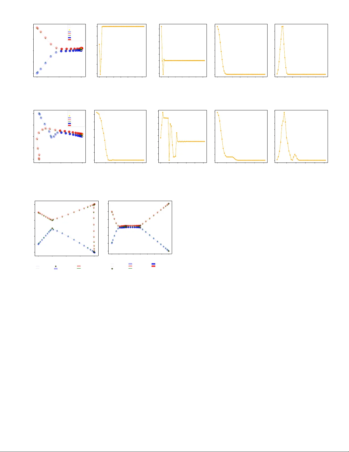
This work has been accepted for publication at the IEEE/ITSS Intelligent T ransportation Systems Conference (ITSC), 2025, ©IEEE Rendezv ous and Docking of Mobile Ground Robots for Ef ficient T ransportation Systems 1 st Lars Fischer FZI Resear ch Center for Information T ec hnology Karlsruhe, Germany lars.fischer@fzi.de 2 nd Daniel Fl ¨ ogel FZI Resear ch Center for Information T ec hnology Karlsruhe, Germany floegel@fzi.de 3 rd S ¨ oren Hohmann Institute of Contr ol Systems Karlsruhe Institute of T ec hnology Karlsruhe, Germany soeren.hohmann@kit.edu Abstract —In-Motion physical coupling of multiple mobile ground robots has the potential to enable new applications like in-motion transfer that improv es efficiency in handling and transferring goods, which tackles current challenges in logistics. A key challenge lies in achieving reliable autonomous in-motion physical coupling of two mobile ground robots starting at any initial position. Existing approaches neglect the modeling of the docking interface and the strategy for approaching it, resulting in uncontrolled collisions that make in-motion physical coupling either impossible or inefficient. T o address this challenge, we propose a central model predictiv e control (MPC) approach that explicitly models the dynamics and states of two omnidir ec- tional wheeled robots, incorporates constraints related to their docking interface, and implements an approaching strategy for rendezv ous and docking. This novel approach enables omnidi- rectional wheeled robots with a docking interface to physically couple in motion regardless of their initial position. In addition, it makes in-motion transfer possible, which is 19.75% more time- and 21.04% energy-efficient compared to a non-coupling approach in a logistic scenario. Index T erms —A utonomous Rendezvous and Docking, In- Motion T ransfer , Physical Coupling, Model Predictive Control. I . I N T R O D U C T I O N The importance of transportation is evident in its role in supporting all economic activities [1]. In the production of goods, for example, material flow requires logistics to ensure the right product is in the right place at the right time [2]. In logistics, autonomous mobile robots (AMR) are often used for transportation due to increased efficienc y compared to humans and thus, play a central role in modern logistic systems [3]. It is further postulated that the optimal logistic space is empty and only AMR swarms are used for transportation [2]. Howe ver , this requires that AMR are able to handle a broad range of tasks in modern logistics [4]. While AMR still struggle with limited flexibility and reconfigurability in respond to changing needs, they are still seen as a key dri ver to gather flexibility and adaptability in transportation [4]. This imposes the need for AMR to be flexible, scalable, and adaptable [2, 5]. Additionally , there is a need to ef ficiently transfer goods while dri ving to reduce occupancy time on loading and unloading areas [5]. Current motion planning approaches commonly implement collision av oidance by defining a safety distance between them [6, 7]. Howe v er , it would be beneficial if they have the Fig. 1. The proposed approach allows robots to physically couple in- motion and enables in-motion transfer . In a logistic scenario, this facilitates transporting packets with the same destination together in bundles, thereby reducing overall tra vel distance, ener gy consumption, and time. ability to physically couple in motion with each other . First, this enables in-motion transfer , the ability to transfer goods while being in motion [8]. Considering a logistic scenario as depicted in Fig. 1, the ability to physically couple enables robots to bundle packets with the same destination, which increases efficienc y . In the mobility domain, in-motion transfer can improve energy consumption, capacity utilization rate, and overall ef ficiency [8]–[10]. Second, physically coupling a robot transporting a workpiece with another robot equipped with a tool enables the processing of workpieces during transportation. Third, skill sets can be broadened, such as increasing maximum payload and loading capacity . Howe v er , this requires robots with the ability to couple in motion physically . Formation control methods that enable logical coupling are commonly used in logistics to implement cooperativ e tasks, e.g., cooperativ e object transportation, where multiple robots carry objects that are either too heavy , too large, or of a complex shape for one robot to transport [6, 11]–[13] Ho we ver , these approaches do not model a docking interface or an approaching strategy , so setting the inter-robot distance to zero in these approaches results in uncontrolled collisions. Besides, some approaches implement physical coupling for mobile ground robots, but either physical coupling is only possible if one agent is static [12, 14, 15] or the feasibility of in-motion physical coupling is dependent on specific initial states [16], which is not efficient. Therefore, there is a gap in the ability of mobile ground robots within the logistics domain to physically couple in motion, which limits their flexibility and adaptability by not enabling use cases like in-motion transfer . T o address these drawbacks, we propose a central model predictive control (MPC) motion planning approach, which includes the imposed constraints of the docking interface and the approaching strat- egy . Therewith, it is achieved that AMR are able to physically couple in motion, regardless of their initial state. The main contribution of this paper is a nov el MPC ap- proach enabling mobile ground robots to physically couple in motion. Therefore, we model and identify the key constraints necessary for the physical coupling of two omnidirectional wheeled robots. Thereby , a constraint optimization problem is formulated for a central MPC, that also captures the approaching strategy . The simulation based analysis demon- strates the feasibility of the proposed approach and shows the effecti v eness compared to a no coupling approach in a logistics scenario. Overall, we make three claims: First, the proposed approach enables in-motion physical coupling of two robots with omni- wheel system dynamics. Second, our approach is v ersatile with respect to different initial states. Third, we claim that the so- enabled use case in-motion transfer is time and energy saving compared to a non-coupling scenario. I I . R E L A T E D W O R K W e define logical coupling as the ability of multiple robots to achie ve a predetermined spatial configuration, which is characterized by a non-zero inter-robot distance. This ability can be enabled by solving a formation control problem [17]. W e define physical coupling as the ability of robots to ex ecute docking operations that, on the one hand, reduce the inter- robot distance up to zero and, on the other hand, physically connect at least two robots. This ability can be enabled by solving a so-called rendezvous and docking problem [18]. In the context of formation control, a rendezvous problem is the name for a consensus problem, a special class of formation control problems [19]. A. Logical Coupling of Mobile Gr ound Robots In [11] an optimal formation for a group of robots is calculated that is used by a distributed model predicti ve control (DMPC) scheme to enable cooperativ e transportation of arbi- trary shaped objects. The DMPC is responsible for maintaining the formation’ s shape and to move the shape along the desired path. A leader-follo wer architecture is used where the leader is a virtual object, and all robots are following this leader with a prescribed pose. A similar virtual leader approach is used in [20], although only one vehicle is controlled. [21] implements a DMPC approach with a virtual leader-follo wer approach that logically couples multiple dif ferentially dri ven robots. [7] implements different DMPC schemes that couple each robot to its neighbor, follo wing each other with a prescribed offset. [6] implements a DMPC for multiple robots transporting a plate. The cost function is designed so that deviations of the desired formation can occur to improv e the trajectory tracking error . These methods ensure formation stability and trajectory or setpoint tracking by controlling a predefined spatial configu- ration. Howe v er , they do not model any docking constraints or approaching strategies, although they are necessary for successful docking operations [18]. Therefore, these formation control approaches are unsuitable for solving our rendezvous problem to enable in-motion physical coupling. B. Physical Coupling of Mobile Gr ound Robots Modular autonomous logistic vehicles designed to logically and physically couple are introduced in [12]. A formation controller is implemented that logically couples the robots to enable collaborativ e transportation. There are two types of modular vehicles introduced, an activ e robot that is equipped with a dri ving unit and a passi ve carrier that does not hav e activ e components. The activ e robot is capable of physically coupling with the passiv e carrier through an electromagnet. Howe v er , they neither in vestigate approaches for in-motion physical coupling nor for static physical coupling, where the activ e robot is dri ving and the other is not. A modular vehicle for a logistic task with omnidirectional dri ve and electromagnets to enable static physical coupling is designed in [14]. For shape reconfiguration, the coupling point is static and is calculated by the position of the target vehicle to be cou- pled with. During reconfiguration, the target vehicle is static while the chasing vehicle is driving. In [15], the trajectory planning is extended with an artificial potential field method that also considers static physical coupling. Indeed, this ap- proach considers docking constraints, but not for a dynamic setting, where a synchronization of velocities and docking directions should be implemented to prev ent frontal collisions. A leader-follo wer consensus algorithm with trajectory tracking is implemented in [22]. The objectiv e is to find a con v ergence point where a group of robots can rendezvous. This approach is not applicable as they do not model the necessary docking interfaces. A PID-based controller is introduced in [16] to physically couple two robots in motion. The drawback of this approach is that there are infeasible initial states if the connection points are on the wrong side of the robot. The controller cannot plan a trajectory around the other robot to couple from the other side. These methods also lack the modeling of any docking constraints or approaching strategies, making them unsuitable for enabling in-motion physical coupling. C. Physical Coupling of Spacecrafts Primarily , there is a need for spacecrafts to hav e the ability to physically couple in motion. Thus, the rendezvous and docking problem is mainly examined and defined there, e ven if there are in vestig ations in other domains [8, 9, 23]. It is a key technology to space missions such as repairing satellites or as- sembling a space station out of modules [24]. The rendezvous and docking is defined in [24] as ”two spacecrafts meet in space with the same velocity and the join into a complex”. Commonly in such space missions, spacecrafts start out of sight of each other , go through several phases to get in close- range, and end in a docking maneuver where they physically couple. In such missions, two actors are defined, the chaser , which is the active part and performs the maneuvers, and the target on which the chaser aims to dock [24, 25]. T o solve rendezvous and docking problems in space, commonly optimal control methods [26] are used, including MPC [27]–[30]. [28] refers to various papers that propose a MPC for close-range rendezvous problems because it can handle constraints in a multiv ariable control system. For further reading on control methods for space rendezvous and docking is referred to [18, 24]. The approaches for physical coupling of spacecrafts do model docking constraints and approaching strategies, making them suitable as a starting point for our work. Howe ver , these approaches require adaptation to be applied to mobile ground robots, as the boundary conditions differ . First, these approaches consider the system dynamics of two spacecraft, which are fundamentally different from those of a mobile ground robot. Secondly , it is necessary to assess which con- straints and approaching strategies from space missions are applicable to mobile ground robots. Thirdly , these approaches assume that only one spacecraft is controllable while the other is passive. In our case, both mobile ground robots are con- trollable, which also influences the design of the approaching architecture. Giv en the constraints imposed by the docking interface and the multiv ariable nature of the control system, employing MPC approach seems appropriate. I I I . C O N S T R A I N T M O D E L I N G F O R O M N I D I R E C T I O NA L - W H E E L E D RO B O T S The problem addressed in this paper is to enable in-motion physical coupling for two omnidirectional wheeled robots with an electromagnet as a docking interface. T o enable this ability , we first model each robot’ s system dynamics to predict the robot’ s states and plan trajectories. Afterwards, we adapt the approaching strategy from space rendezvous and docking for mobile ground robots to achie v e reliable and unambiguous approaching. Lastly , all necessary constraints imposed by the docking interface are derived to ensure feasibility for all initial poses. A. System Dynamics T wo wheeled mobile robots with the same system dynamics on a two-dimensional free plane are considered. W e assume omnidirectional wheeled robots since they are widespread in logistics [6, 12, 14, 31, 32]. Each robot i is modeled as a disk with radius r . The pose of robot i is described by the center point of the disk with x-position p i x ∈ R , y-position p i y ∈ R and heading θ i k ∈ [0 , 2 π ) in global reference system O g and leads to the state vector x i =  p i x p i y θ i  T (1) at time k . Both robots can be controlled individually with translational velocity in the x-direction v i x and the y-direction v i y as well as the angular velocity ω i . This results in the input vector u i =  v i x v i y ω i  T (2) of robot i at time k . In real-world scenarios, all actuators are limited due to physical constraints or energy limitations. Thus, we define the maximal control inputs as u i ≤ u i max (3) The discrete system dynamic for an omnidirectional wheeled mobile robot is deriv ed by Euler-Forward x i k +1 = x i k + ∆ T · u i k (4) B. Docking Interface The implementation of a coupling interface can be, for example, an electromagnet or a mechanical closure [33]. W e consider an electromagnet as a docking interface and model it as a rectangle on the margin of the robot. The direction of the coupling interface is set by the parameter δ φ,i ∈ [ − π , π ) that denotes the orientation shift of the coupling interface in reference to the heading θ i (cf. Fig. 2). The heading θ i d ∈ [0 , 2 π ) of the docking interface is defined by θ i d = θ i + δ φ,i (5) The center point p i d ∈ R 2 of the docking interface is defined by p i d =  p i x + r · cos θ i d p i y + r · sin θ i d  (6) Fig. 2 illustrates the modeled robot with its docking interface. The robot is depicted as a grey circle with a black mar gin. The docking interface is depicted as a green rectangle on the margin. x y O g ( p i x , p i y ) θ i θ i d δ φ,i Fig. 2. Illustration of the robot modeling. Robot i is a grey disk with radius r ( ). The heading θ i is depicted as a blue arrow ( → ). The docking interface is located on the margin of the disk and depicted as a green rectangle ( ■ ). The heading of the docking axis is depicted as a green arrow ( → ). C. Appr oaching Strate gy The approaching strategy is mainly deri ved from a common rendezvous and docking mission in space, where the approach- ing strategy can be di vided into se veral phases [18, 24, 25]. Not all phases are rele v ant for the considered problem here, as we assume, for example, that the mobile robots are initialized in line of sight, in contrast to a space mission. Thus, our problem does not cover the phases launch and phasing , where the main goal is to get into a stable state and in line of sight. W e deri ve three main phases for the physical coupling of AMR. The first phase is called far rang e rendezvous , where the goal is to approach the first aim point. In our case, this is the approaching of the docking axis. The proposed strategy is that robot 2 aims for the docking axis of robot 1 and concurrently aligns its docking axis to that of robot 1. This also aligns the coupling interfaces. The second phase is called close range rendezvous , which is di vided into the two sub phases closing and final approac h . The closing reduces the distance between the coupling in- terfaces and acquires conditions to allow the final approach. In our conte xt, this phase is about approaching the docking corridor and reducing the relative velocity between the robots. The final approach is about achieving the docking, where the coupling interfaces touch each other, and the approaching corridor constrains the mov ements. The third and last phase is docking , where the capture is achiev ed. In this conte xt, we assume an electromagnet to achiev e docking. D. Physical Coupling Constraints W e derive the relev ant physical coupling constraints mainly from the rendezvous and docking mission from space and adapt them to mobile ground robots. Concerning the ap- proaching strategy , each phase imposes dif ferent constraints that must be modeled and considered in the approach to achiev e docking in motion. Reg arding the far range rendezv ous phase, we need a description of the docking axis and the relativ e position of one robot to the docking axis. For the closing phase, we need a description of the alignment of the docking interface, the relati ve distance between the robots, and the relati ve velocity to enable soft-docking. For the final approach phase, the approaching corridor has to be modeled. The docking phase itself does not impose any constraints, but prohibits the coupled system to hav e slack in the coupling constraints afterwards. 1) Docking Axis Constraint: The approaching direction and the position to be approached depend on both robots’ positions and the orientation of the installed coupling interf ace. The docking axis constraint is introduced to ensure that the robots couple from a feasible direction (cf. Fig. 3). First, we define the angle φ 12 ∈ [0 , 2 π ) in reference to the x-axis of the vector that starts at robot 1 and ends at robot 2. φ 12 = atan2( p 2 y − p 1 y , p 2 x − p 1 x ) (7) Thereby , it is possible to describe the de viation of the position of robot 2 from the docking axis of robot 1 by building the difference between θ 1 d and φ 12 . This de viation has to be zero for physical coupling and leads to the constraint θ 1 d − φ 12 | {z } I = 0 (8) 2) Alignment Constraint: While the docking axis constraint (8) only aligns the position of robot 2 with the docking axis of robot 1, the alignment of the docking interfaces is lacking. Follo wing [16], a heading alignment constraint can be used to control the alignment of the coupling interfaces. As an alignment of the coupling interface is obtained, the heading of the docking interface is used instead of the heading of the robots. The coupling interfaces are aligned if their docking axes point at each other . For the mathematical modeling, the difference between the docking axis heading ∆ θ d is mapped to values from [0 , π ] . ∆ θ d = θ 1 d − θ 2 d (9) The docking axes are pointing at each other , if ∆ θ d equals π , which leads to the alignment constraint ∆ θ d − π | {z } I I = 0 (10) 3) Relative Distance Constraint: The relati ve distance be- tween the robots is defined by the distance of their center point. T o enable the docking operation, the relativ e distance between both robots has to be the sum of the distance of the modeled disk radius r and thus leads to ( p 1 x − p 2 x ) 2 + ( p 1 y − p 2 y ) 2 − δ r | {z } I I I = 0 (11) [16] proposes a similar constraint for mobile ground robots. The parameter δ r ∈ [0 , ∞ ) defines the relativ e distance. 4) Soft-Docking Constraint: In order to prevent damage, the force transmission should be as small as possible which is why the relative velocity and acceleration of the robots hav e to be constrained to a minimum while docking. Follo wing [27], a soft-docking constraint is formulated to lower the relati ve velocity of the robots as they are approaching each other with ( v 1 x − v 2 x ) 2 + ( v 1 y − v 2 y ) 2 | {z } I V = 0 (12) 5) Appr oaching Corridor: T o pre v ent robot 2 from col- liding with robot 1 during approaching the docking axis of robot 1, collision av oidance is considered in the constraints. Therefore, a disk with radius r ca is defined around the center point of robot 1 that is prohibited to enter (cf. Fig. 3). This means that the euclidean distance between the center points of both robots has to be greater than r ca . This is expressed via the collision av oidance term α ca with α ca = (( p 1 x − p 2 x ) 2 + ( p 1 y − p 2 y ) 2 − r 2 ca ) ≥ 0 (13) Having only this constraint would be too restrictiv e, because a physical coupling would be impossible. In the space domain, existing approaches create an interruption in the collision av oidance perimeter at the designated docking axis where it is allo wed to enter [26]. The aperture angle of the corridor is defined around the docking axis by the parameter ∆ φ (cf. Fig. 3). The deviation from the docking axis is defined by ∆ θ φ and mapped to [0, π ]. ∆ θ φ = θ 1 d − φ 12 (14) For reasons of numerical stability , a continuously differentiable function is preferred over a discrete function in the constraints. Thus, tangens hyperbolicus is used instead of a step function to decide whether robot 2 is inside or outside of the corridor . For all de viations from the docking axis that are smaller than ∆ φ , the term within tanh becomes negati ve and thus tanh becomes -1. For all de viations from the docking axis that are greater than ∆ φ , the term within tanh becomes positiv e and thus tanh becomes 1. The hyperparameter l is used to tune the gradient of the tangens hyperpolicus. While increasing l , the tangens hyperbolicus approximates a step function. α ce = (1 + tanh( l · (∆ θ φ − ∆ φ ))) (15) Thereby , the docking corridor term α dc is zero if robot 2 is within the cone and two if robot 2 is outside of the cone. In order to connect (13) with (15) we have to multiply α ca with α ce . 0 ≤ α ca · 1 2 α ce (16) As soon as robot 2 is inside the cone α ce becomes zero, and so α ca is inacti ve. While robot 2 is outside the cone α ce is 2 and α ca is activ e. According to [18], the half cone angle of the approach corridors are arbitrary but for spacecrafts the angle may v ary between ± 5 ◦ and ± 15 ◦ . θ 1 d θ 2 d ∆ θ φ φ 12 ∆ φ Fig. 3. Illustration of the approaching corridor and the docking axis dis- placement. The robots are depicted as grey disk ( ). The docking interface is located on the margin of the disk and depicted as a green rectangle ( ■ ). The heading of the docking axis is depicted as a green arro w ( → ). The approaching corridor is depicted as a green zone around around the docking axis( ). The collision av oidance zone is depicted as a red zone ( ) I V . M O D E L P R E D I C T I V E C O N T R O L L E R D E S I G N Our approach inv olv es designing a central model predictiv e controller that calculates optimal trajectories based on physical coupling. W e now define the cost function and constraints so that the physical coupling constraints are met, the approaching strategy is implemented, and the user-gi v en waypoints are approached physically coupled. A. Slack V ariables Considering the approaching strategy III-C, dif ferent con- straints should be met in different phases. In the final approach phase, right before docking, all constraints from all phases hav e to be met. Howe ver , all constraints cannot be fulfilled from the very beginning, thus slack v ariables ϵ ∈ R 4 are introduced. ϵ k =  ϵ δ r ϵ δ θ ϵ δ v ϵ δ φ  T (17) Adding slack variables in the constraints can soften state constraints so that the slack variable behav es like a decision variable [34]. The individual constraints can be prioritized depending on how the slack variables are penalized in the cost function. The physical coupling constraint equations (8) to (12) are augmented by the inclusion of their related slack variable. If ϵ takes the value zero, the constraint is satisfied. The greater the value of | ϵ | , the more the constraint is violated. The slack variable gi ves the MPC a degree of freedom to driv e the system into a state where the constraints are satisfied by minimizing epsilon in the cost function. T o ensure that already satisfied constraints are maintained, we have to constrain the slack variables to a maximum value ϵ max ∈ R 4 | ϵ | ≤ ϵ max . (18) B. Modeling Central System Dynamics W e consider a central MPC architecture with global infor - mation. For the dynamical model, all states of each robot are considered. Therefore, we define the e xtended state vector z k ∈ R 6 and the extended input vector ν k ∈ R 6 with the central discrete system dynamics z k +1 ∈ R 6 . z k = x 1 k x 2 k ! (19) ν k = u 1 k u 2 k ! (20) z k +1 = f ( z k , ν k ) = z k + ∆ T · ν k (21) C. Cost Function The objective of the MPC is to minimize the slack variables that depict the error of the coupling constraints and to mini- mize the distance to a common way point. So that the robots arriv e at the waypoint physically coupled without stopping in between, we have to penalize the error and thus the slack variables of the coupling constraints more than the distance to the waypoint. Consequently , we introduce the parameter vector λ ∈ R 6 with which we can adjust the weighting of the cost function. λ =  λ δ r λ δ θ λ δ v λ δ φ λ j λ ω  T (22) T o satisfy ev ery constraint, all slack v ariables have to be zero. Hence, the cost function for the coupling constraint L cc is defined as the parameterized weighted sum of the squared slack variable over all timesteps N within the time horizon. L cc ( ϵ k ) = λ δ r · N X k =1 ϵ 2 δ r , k + λ δ Θ · N X k =1 ϵ 2 δ Θ , k + λ δ v · N X k =1 ϵ 2 δ v ,k + λ δ φ · N X k =1 ϵ 2 δ φ , k (23) T o smooth the input variables the deri v ati ves of the inputs are penalized via L in ( ν k ) = λ j · N − 1 X k =0 ( ¨ v 1 x,k ) 2 + ( ¨ v 1 y ,k ) 2 + ( ¨ v 2 x,k ) 2 + ( ¨ v 2 y ,k ) 2 λ ω · N − 1 X k =0 ( ˙ ω 1 k ) 2 + ( ˙ ω 1 k ) 2 (24) The distance between robot 1 and the common waypoint is defined by the euclidean distance. W e use the squared distance, because it provides better numerical performance while not loosing its interpretation. The costs for arriving at the w aypoint L g are formulated as end costs with the weighting parameter λ g ∈ R 6 L g ( z k ) = λ g · ( z N − z soll ) 2 (25) The total costs L result from the sum of coupling costs and waypoint costs. L ( z k , ν k , ϵ k ) = L cc ( ϵ k ) + L in ( ν k ) + L g ( z k ) (26) D. Optimization Pr oblem Putting all together, the MPC minimizes at each time step the cost function L for a time horizon N as defined in (27). The cost function is subject to the central system dynamics z k +1 and the physical coupling constraints. The optimized variables are the states z ∗ 1 → N ∈ R 6 × N , the input variables ν ∗ 0 → N − 1 ∈ R 6 × N and the slack v ariables ϵ ∗ 1 → N ∈ R 4 × N . Hence, the optimization problem is as follows. arg min z k , ν k , ϵ k L ( z k , ν k , ϵ k ) subj. to z k +1 = f ( z k , ν k ) k = 0 , ..., N − 1 z 0 ∈ R 6 I = ϵ δ φ ,k k = 1 , ..., N I I = ϵ δ θ ,k k = 1 , ..., N I I I = ϵ δ r ,k k = 1 , ..., N I V = ϵ δ v ,k k = 1 , ..., N | ϵ | ≤ ϵ max k = 1 , ..., N ν k ≤ ν max k = 0 , ..., N − 1 0 ≤ α ca · 1 2 α ce k = 1 , ..., N (27) V . E V A L UA T I O N This section ev aluates the proposed MPC motion planning approach to enable physical in-motion coupling of AMR. W e first describe the e xperimental setup used to v alidate the claims and subsequently present the simulati ve results. In addition, we discuss and interpret the results and findings. A. Experimental Setup For each claim, we consider one experiment. In the first experiment, we validate the claim that the two omnidirectional robots can physically couple in motion before reaching the goal. Therefore, we set the goal state for robot 1 to [4 , 0 , 0] . The goal state of robot 2 results from the coupling constraints to [4 , 2 , 0] . Robot 1 starts at [0 , − 2 , 0] and Robot 2 at [0 , 2 , 0] , and they are not physically coupled in the beginning, but the docking axes are aligned. This represents the simplest case, and the robots should couple before arri ving at their goal point. The second experiment v alidates the claim that the approach can handle a scenario where the docking axes are not aligned initially . W e use the same goal states as in the first experiment, but the start states of the robots are interchanged. The third experiment validates the claim that the enabled in- motion transfer saves time and energy for a transportation sce- nario in a logistic context. Therefore, we define two scenarios, one without coupling and thus without in-motion transfer and the other with physical coupling and in-motion transfer (cf. Fig. 1). Robot 2 carries two packages, one with destination A = (8 , 2) and the other with destination B = (8 , − 2) . Robot 1 only carries a package with destination B . The initial states of the robot are the same as in experiment 1. For both scenarios, the first waypoint is [2 , 0] for robot 1 and [2 , 1] for robot 2, as we assume the robots are driving out a shelf row . In the approach with coupling, robot 2 transfers the package for destination B to robot 1. The scenarios end if both robots hav e deli vered their packages. In all experiments, the docking axis for robot 1 is set to δ φ, 1 = 90 and for robot 2 to δ φ, 2 = − 90 . Both robots are modeled as a disk with r = 0 . 1 and thus δ r = 0 . 2 . The approaching corridor is set to ∆ φ = 15 . Considering the approaching strategy the weighting of the cost function is set to λ = [30 , 1000 , 1 , 200 , 0 . 1 , 1] T . The MPC hyperparameters are the time horizon T = 5 and the steps N = 20 . The end costs are set to λ g = [1 , 1 , 200 , 1 , 1 , 200] . The algorithm is implemented with python and casadi [35] and solv ed with ipopt. B. Results The results of experiment 1 are depicted in Fig. 4. Fig. 4a shows the temporal course of the global position of robot 1 depicted in blue and robot 2 depicted in red. The docking axis is marked in green, and the goal position is depicted as a yellow star . The robots are displayed in non-transparent color once they are physically coupled. Both robots start at their initial position and drive to their goal point while satisfying the coupling constraints. This is depicted by the decreased value of the slip variables over time. The slip in the docking axis (cf. Fig. 4b) and the alignment (cf. Fig. 4c) constraint go tow ards zero first. Afterwards, the slip in the relativ e distance (cf. Fig. 4d) goes tow ards zero. The slip in the soft-docking constraint is increasing first before decreasing to zero (cf. Fig. 4e). After 2 seconds, both robots are physically coupled and are driving to their goal state together . The results of e xperiment 2 are depicted in Fig. 5. Fig. 5a shows the temporal course of the global position of the robots analogous to Fig. 4a. The slip of the docking axis is monotonously decreasing (cf. Fig.5b). The slip of the alignment of the docking axes is oscillating around zero before con v erging to it (cf. Fig.5c). The relativ e distance is decreasing first, but after 2 seconds it remains on a plateau before it decreases towards zero after 3.5 seconds (cf. Fig.5d). The slip of the soft-docking constraint shows two hills, one after 1.5 seconds and the other after 3.75 seconds (cf. Fig. 5e). The results of experiment 3 are depicted in Fig. 6. Fig. 6a shows the temporal course of the global position of both robots that do not perform any coupling. In this no coupling scenario, robot 2 is driving to both goal points A and B whereas robot 1 only dri ves to B . Fig. 6b shows the scenario with physical coupling and in-motion transfer . Here, the robots are coupled for 7 seconds before they uncouple. W ithin that time, in- motion transfer can be carried out, before they uncouple. So, T ABLE I E X PE R I M EN T 3 - A G G R EG ATE D NA V IG ATI O N M E T RI C S Approach T ime (s) Energy (J) Distance (m) No coupling 20.25 10.49 30.2 Ours: with coupling 16.25 8.28 25.51 robot 2 can transfer its package with destination B to robot 1 which is why robot 2 driv es only to A and robot 1 only to B . A comparison of the navigation metrics of experiment 3 is depicted in T ab . I. Our approach enables physical coupling and thus in-motion transfer , which outperforms a no coupling scenario in terms of total time, total energy , and total distance in a simple scenario. Our approach improv es total time by 19.75 %, total ener gy by 21.04 % and total distance by 15.52 % compared to a no coupling scenario in experiment 3. C. Discussion The results sho w that the approach is capable of physi- cally coupling two omnidirectional wheeled robots in motion. Moreov er , the approach can handle initial states where the docking axes are not perfectly aligned. This can be seen with the aid of Fig. 5b and 5d. Robot 2 has to be in the approach corridor before the relative distance can go to zero. That is why Fig. 5d has a plateau after 2 seconds but decreases after 3.75 seconds, because it is in the docking corridor then. The soft-docking constraint is the only constraint that increases during the optimization. But, that has to be the case so that the distance decreases, because a high slip in the soft-docking means driving to wards each other . The simple logistic scenario demonstrates ener gy and time efficienc y and v alidates that physical coupling can increase efficiency in a logistic scenario. Howe v er , the approach has only been tested in a simula- tion. Real-world experiments should be conducted to analyze the performance of our approach with measurements. More experiments could be done with other system dynamics like differential dri ve or ackermann kinematic, to ev aluate the feasibility for other system dynamics. V I . C O N C L U S I O N S In this paper , a central MPC for in-motion physical coupling of mobile ground robots has been designed and implemented in a simulation. Thereby , we deri v ed an approach for in-motion physical coupling for omnidirectional wheeled robots. The results v alidate our approach and demonstrate that in-motion physical coupling of robots is preferable to no coupling in a logistic scenario, as it increases efficienc y through in-motion transfer . Consequently , our approach can be applied to similar modular robots in a logistic context to enhance efficienc y by providing the baseline for in-motion transfer and sorting. Moreov er , this approach can be transferred to the mobility sector to enhance ef ficiency of autnonomous modular pods. Further work incorporates an e v aluation in real world. R E F E R E N C E S [1] S. Sivanandham and M. S. Gajanand, “Platooning for sustainable freight transportation: An adoptable practice in the near future?” T ransport Reviews , vol. 40, no. 5, pp. 581–606, Jan. 2020. [2] T . Bauernhansl, M. T en Hompel, and B. V ogel-Heuser, Eds., Industrie 4.0 in Produktion, Automatisierung und Logistik: Anwendung · T ech- nologien · Migration . Springer Fachmedien W iesbaden, 2014. [3] H. Pikner, R. Sell, K. Karjust, E. Malayjerdi, and T . V elsker , “Cyber- physical Control System for Autonomous Logistic Robot, ” in 2021 IEEE 19th International P ower Electronics and Motion Contr ol Conference (PEMC) . IEEE, Jan. 2021, pp. 699–704. [4] L. Heuss, A. Blank, S. Dengler, G. L. Zikeli, G. Reinhart, and J. Franke, “Modular Robot Software Frame work for the Intelligent and Flexible Composition of Its Skills, ” in Advances in Pr oduction Management Systems. Pr oduction Management for the F actory of the Futur e , ser . IFIP Advances in Information and Communication T echnology , F . Ameri, K. E. Stecke, G. Cieminski, and D. Kiritsis, Eds. Cham: Springer International Publishing, Jan. 2019, vol. 566, pp. 248–256. [5] SP ARC, “H2020 Robotics Multi-Annual Roadmap ICT -2017B, ” T ech. Rep., 2017. [6] H. Ebel, E. Sharafian Ardakani, and P . Eberhard, “Distributed model predictiv e formation control with discretization-free path planning for transporting a load, ” Robotics and Autonomous Systems , vol. 96, pp. 211–223, Jan. 2017. [7] G. Stomberg, H. Ebel, T . Faulw asser , and P . Eberhard, “Cooperative dis- tributed MPC via decentralized real-time optimization: Implementation results for robot formations, ” Contr ol Engineering Practice , vol. 138, p. 105579, Sep. 2023. [8] Z. S. Khan, W . He, and M. Men ´ endez, “ Application of modular vehicle technology to mitigate bus bunching, ” Tr ansportation Researc h P art C: Emer ging T ec hnologies , vol. 146, p. 103953, Jan. 2023. [9] J. W u, B. Kulcs ´ ar , Selpi, and X. Qu, “ A modular , adaptiv e, and autonomous transit system (MAA TS): An in-motion transfer strategy and performance evaluation in urban grid transit networks, ” Tr ansportation Resear ch P art A: P olicy and Practice , vol. 151, pp. 81–98, Jan. 2021. [10] Z. Zhang, A. T afreshian, and N. Masoud, “Modular transit: Using auton- omy and modularity to improve performance in public transportation, ” T r ansportation Resear ch P art E: Logistics and T r ansportation Revie w , vol. 141, p. 102033, Jan. 2020. [11] H. Ebel and P . Eberhard, “Optimization-Dri ven Control and Or ganization of a Robot Swarm for Cooperativ e T ransportation, ” IF AC-P apersOnLine , vol. 52, no. 15, pp. 115–120, Jan. 2019. [12] M. Hompel et al., “T echnical Report: LoadRunner®, a new plat- form approach on collaborative logistics services, ” W issenschaftliche Gesellschaft f ¨ ur T echnische Logistik, T ech. Rep., Jan. 2020. [13] E. T uci, M. H. M. Alkilabi, and O. Akanyeti, “Cooperative Object T ransport in Multi-Robot Systems: A Review of the State-of-the-Art, ” F r ontiers in robotics and AI , vol. 5, p. 59, Jan. 2018. [14] J. Zhou et al., “Design, Fabrication, and Control Algorithm of Self- Reconfigurable Modular Intelligent V ehicles, ” Applied Sciences , vol. 12, no. 14, p. 6886, Jan. 2022. [15] J. Zhou, J. W ang, J. He, J. Gao, A. Y ang, and S. Hu, “ A Reconfigurable Modular V ehicle Control Strategy Based on an Improv ed Artificial Potential Field, ” Electronics , vol. 11, no. 16, p. 2539, Jan. 2022. [16] S. Y i, Z. T emel, and K. Sycara, “Configuration Control for Physical Coupling of Heterogeneous Robot Swarms, ” in 2022 International Confer ence on Robotics and Automation (ICRA) . Philadelphia, P A, USA: IEEE, May 2022, pp. 4268–4274. [17] H.-S. Ahn, F ormation Control: Appr oaches for Distributed Agents , ser . Studies in Systems, Decision and Control. Cham: Springer International Publishing, 2020, vol. 205. [18] W . Fehse, Ed., Automated Rendezvous and Docking of Spacecraft , ser . Cambridge Aerospace Series. Cambridge New Y ork: Cambridge Univ ersity Press, 2003, no. 16. [19] K.-K. Oh, M.-C. Park, and H.-S. Ahn, “ A survey of multi-agent formation control, ” Automatica , vol. 53, pp. 424–440, Mar . 2015. [20] M. Egerstedt, X. Hu, and A. Stotsky , “Control of mobile platforms using a virtual vehicle approach, ” IEEE Tr ansactions on Automatic Control , vol. 46, no. 11, pp. 1777–1782, Nov . 2001. [21] M. Rosenfelder , H. Ebel, and P . Eberhard, “Cooperativ e distributed nonlinear model predictive control of a formation of differentially-dri ven mobile robots, ” Robotics and Autonomous Systems , vol. 150, Jan. 2022. [22] A. Patil and G. Shah, “Multi-Robot Trajectory T racking and Rendezvous Algorithm, ” IETE J ournal of Researc h , vol. 68, no. 6, pp. 4570–4576, Jan. 2022. [23] Z. Jia, H. Lu, H. Chen, and W . Zhang, “Robust Distributed Cooper- ativ e Rendezvous Control for Heterogeneous Marine V ehicles Using 0 1 2 3 4 X (m) − 2 − 1 0 1 2 Y (m) Path Robot 1 Path Robot 2 Goal Robot 1 uncoupled Robot 2 uncoupled Docking Axis Robot 1 coupled Robot 2 coupled 1 (a) Global Position 0 2 4 6 8 10 12 t (s) −0.005 −0.004 −0.003 −0.002 −0.001 0.000 ε δ φ (b) Slip Docking Axis 0 2 4 6 8 10 12 t (s) − 0.00050 − 0.00025 0.00000 0.00025 0.00050 0.00075 0.00100 0.00125 ϵ δ θ 1 (c) Slip Alignment Docking In- terface 0 2 4 6 8 10 12 t (s) 0 2 4 6 8 10 12 14 16 ϵ δ r 1 (d) Slip Relativ e Distance 0 2 4 6 8 10 12 t (s) 0 1 2 3 4 5 ϵ δ v 1 (e) Slip Soft-Docking Fig. 4. Experiment 1 - The robots’ docking axes are perfectly aligned at the beginning. The goal is that the robots satisfy the coupling constraints before arriving at the goal point and thus physically couple in motion. 0 1 2 3 4 X (m) −2 −1 0 1 2 Y (m) Path Robot 1 Path Robot 2 Goal Robot 1 uncoupled Robot 2 uncoupled Docking Axis Robot 1 coupled Robot 2 coupled (a) Global Position 0 2 4 6 8 10 t (s) 0.0 0.5 1.0 1.5 2.0 2.5 3.0 ε δ φ (b) Slip Docking Axis 0 2 4 6 8 10 t (s) − 0.0075 − 0.0050 − 0.0025 0.0000 0.0025 0.0050 0.0075 0.0100 0.0125 ϵ δ θ 1 (c) Slip Alignment Docking In- terface 0 2 4 6 8 10 t (s) 0 2 4 6 8 10 12 14 16 ϵ δ r 1 (d) Slip Relativ e Distance 0 2 4 6 8 10 t (s) 0 1 2 3 4 5 6 7 8 ϵ δ v 1 (e) Slip Soft-Docking Fig. 5. Experiment 2 - The robots’ docking axes are not aligned at the beginning. The goal is that the robots satisfy the coupling constraints before arriving at the goal point and thus physically couple in motion. 0 2 4 6 8 X (m) − 3 − 2 − 1 0 1 2 3 Y (m) A B Path Robot 1 Path Robot 2 Goal Robot 1 uncoupled Robot 2 uncoupled Docking Axis 1 (a) No coupling 0 1 2 3 4 5 6 7 8 X (m) − 3 − 2 − 1 0 1 2 3 Y (m) A B Path Robot 1 Path Robot 2 Goal Robot 1 uncoupled Robot 2 uncoupled Docking Axis Robot 1 coupled Robot 2 coupled 1 (b) Rendezvous and Docking with in- motion transfer Fig. 6. Experiment 3 - A comparison is performed between a no coupling scenario and a physically coupling scenario with in-motion transfer . Robot 1 only has to deliver a package to point B . Robot 2 has to deliver two packages, one to point A and B . In the no coupling scenario, robot 2 has to drive to both destinations, whereas in the physically coupling scenario, robot 2 only has to driv e to A because the package can be transferred to robot 1 due to the so enabled in-motion transfer . Model Predictive Control, ” IEEE T ransactions on V ehicular T ec hnology , vol. 73, no. 8, pp. 11 002–11 013, Aug. 2024. [24] Y . Luo, J. Zhang, and G. T ang, “Survey of orbital dynamics and control of space rendezvous, ” Chinese J ournal of Aer onautics , vol. 27, no. 1, pp. 1–11, Feb . 2014. [25] J. R. W ertz and R. Bell, “ Autonomous rendezvous and docking tech- nologies: Status and prospects, ” in AeroSense 2003 , P . Tchoryk, Jr . and J. Shoemaker , Eds., Orlando, FL, Aug. 2003, pp. 20–30. [26] Y . Zhang, B. Zhu, M. Cheng, and S. Li, “T rajectory optimization for spacecraft autonomous rendezvous and docking with compound state- triggered constraints, ” Aerospace Science and T echnology , vol. 127, p. 107733, Aug. 2022. [27] S. Di Cairano, H. Park, and I. Kolmanovsk y , “Model Predictiv e Control approach for guidance of spacecraft rendezvous and proximity maneu- vering, ” International Journal of Robust and Nonlinear Contr ol , vol. 22, no. 12, pp. 1398–1427, Aug. 2012. [28] Q. Li, J. Y uan, B. Zhang, and C. Gao, “Model predictiv e control for autonomous rendezvous and docking with a tumbling target, ” Aer ospace Science and T echnology , vol. 69, pp. 700–711, Oct. 2017. [29] A. W eiss, M. Baldwin, R. S. Erwin, and I. Kolmano vsky , “Model Predictiv e Control for Spacecraft Rendezvous and Docking: Strategies for Handling Constraints and Case Studies, ” IEEE T ransactions on Contr ol Systems T echnology , vol. 23, no. 4, pp. 1638–1647, Jul. 2015. [30] L. Ravikumar , N. K. Philip, R. Padhi, and M. S. Bhat, “ Autonomous terminal maneuver of spacecrafts for rendezvous using model predictive control, ” in 2016 Indian Control Conference (ICC) . Hyderabad, India: IEEE, Jan. 2016, pp. 72–78. [31] H. Eschmann, H. Ebel, and P . Eberhard, “High Accuracy Data-Based T rajectory Tracking of an Omnidirectional Mobile Robot, ” vol. 120, pp. 420–427, Jan. 2022. [32] A. Colomb and C. Brenner , “Konzept zur intuitiv en steuerung omni- direktionaler flurf ¨ orderzeuge mit beliebiger radkonfiguration, ” Logistics Journal: re viewed , no. 12, 2020. [33] H. ˙ I. Dokuyucu and N. G. ¨ Ozmen, “ Achievements and future direc- tions in self-reconfigurable modular robotic systems, ” Journal of Field Robotics , vol. 40, no. 3, pp. 701–746, Jan. 2023. [34] J. B. Rawlings, D. Q. Mayne, and M. M. Diehl, “MPC-book-2nd-edition- 4th-printing, ” Apr. 2022. [35] J. A. E. Andersson, J. Gillis, G. Horn, J. B. Rawlings, and M. Diehl, “CasADi: A software framework for nonlinear optimization and optimal control, ” Mathematical Pr ogr amming Computation , vol. 11, no. 1, pp. 1–36, Mar . 2019.