Understanding the Curse of Unrolling

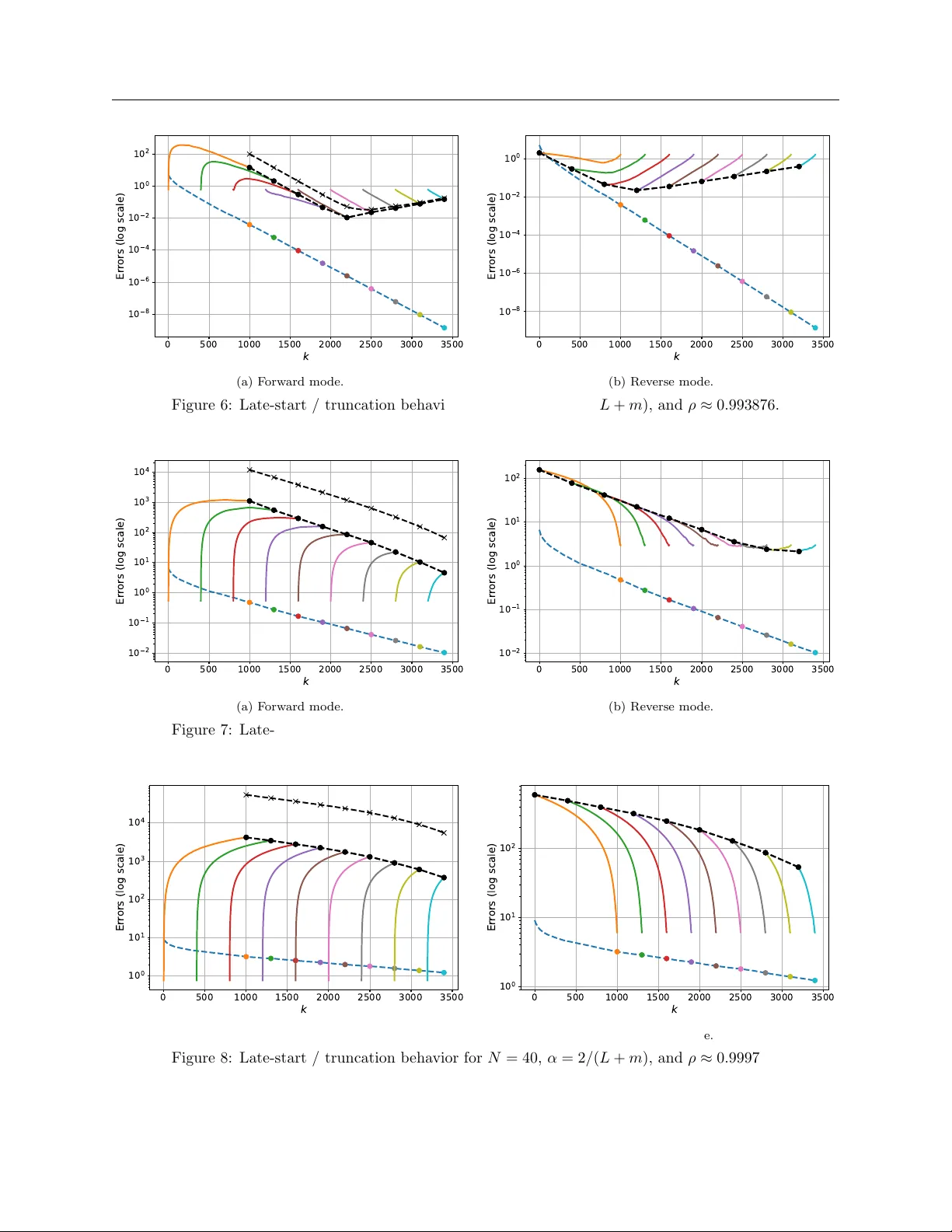
Understanding the Curse of Unrolling Shehery ar Mehmo o d † and Florian Knoll ⋆ and P eter Oc hs † † Saarland Univ ersity , Saarbr ¨ uc ken, German y ⋆ F riedrich-Alexander Univ ersit y , Erlangen, German y Abstract Algorithm unrolling is ubiquitous in mac hine learning, particularly in h yp erpa- rameter optimization and meta-learning, where Jacobians of solution mappings are computed b y differentiating through iterativ e algorithms. Although unrolling is kno wn to yield asymptotically correct Jacobians under suitable conditions, recent work has sho wn that the deriv ativ e iterates may initially diverge from the true Jacobian, a phe- nomenon known as the curse of unrolling. In this work, we provide a non-asymptotic analysis that explains the origin of this b ehavior and iden tifies the algorithmic factors that gov ern it. W e sho w that truncating early iterations of the deriv ative computa- tion mitigates the curse while simultaneously reducing memory requirements. Finally , w e demonstrate that w arm-starting in bilevel optimization naturally induces an im- plicit form of truncation, pro viding a practical remedy . Our theoretical findings are supp orted by numerical exp eriments on representativ e examples. 1 In tro duction Man y problems in mo dern machine learning can b e form ulated as bilevel optimization tasks [ 16 , 17 ], where an outer ob jectiv e dep ends on the solution of an inner problem. That is, giv en a sufficien tly smo oth mapping ℓ : X × U → R , we solv e min u ∈U ℓ ( x ⋆ ( u ) , u ) , (1) where, for eac h parameter v ector u , the quan tit y x ⋆ ( u ) is defined implicitly as the solution of an optimization problem or, more generally , as the solution of a nonlinear equation in the v ariable x . Suc h form ulations arise in a wide range of applications, including hyperparameter optimization [ 9 , 28 , 35 ], meta-learning [ 10 , 26 , 38 ], implicit deep learning [ 2 , 4 , 6 , 7 ], and neural arc hitecture searc h [ 27 ]. In this w ork, w e fo cus on deterministic settings in whic h x ⋆ ( u ) is c haracterized as the fixed p oin t of a smo oth parameterized mapping A : X × U → X , that is, x ⋆ ( u ) solv es x = A ( x , u ) . (2) Intr o duction 0 200 400 600 800 1000 k 1 0 3 1 0 2 1 0 1 1 0 0 Er r ors (log scale) x ( k ) ( u ) x * ( u ) D x ( k ) ( u ) D x * ( u ) k Figure 1: Iterate x ( k ) ( u ) vs deriv ative D x ( k ) ( u ) error plot for gradien t descen t applied to f ( x , u ) : = ∥ A x − b ∥ 2 / 2 + u ∥ x ∥ 2 / 2. Unlike x ( k ) ( u ), D x ( k ) ( u ) initially drifts aw a y from its limit b efore ev en tually coming bac k to it. W e provide a non-asymptotic understanding of this transien t behavior, called the curse of unrolling, and study simple w ays to mitigate it. for x ∈ X . This formulation serv es as the fixed-p oin t equation of many iterativ e algorithms used in practice, such as, gradient descen t, to solv e inner problems of the form min x ∈X f ( x , u ) . (3) Under standard assumptions, the solution x ⋆ ( u ) of ( 2 ) or ( 3 ) exists, is unique, and dep ends smo othly on u . T o solv e the bilev el problem using gradient-based metho ds, we need to compute the gradien t of the outer ob jectiv e ℓ ( x ⋆ ( u ) , u ) with respect to the parameter u . By the c hain rule, this requires the deriv ativ e of the solution map x ⋆ ( u ) with resp ect to u . When x ⋆ ( u ) is defined implicitly as the fixed point of A , this deriv ativ e can be c haracterized using the implicit function theorem. Under suitable regularity conditions (see Theorem 2 ) on A or the inner ob jectiv e f , the map u 7→ x ⋆ ( u ) is differentiable and its Jacobian is giv en b y D x ⋆ ( u ) : = ( I − D x A ( x ⋆ ( u ) , u )) − 1 D u A ( x ⋆ ( u ) , u ) . This approac h, commonly referred to as implicit differentiation, has b ecome a standard to ol for computing gradients in bilevel optimization and related problems. In practice, since the — 2 — Contributions exact fixed p oint x ⋆ ( u ) is rarely av ailable, implicit differentiation is t ypically applied b y replacing x ⋆ ( u ) with an appro ximate solution obtained after a finite n um b er of iterations of an inner algorithm. In practice, the solution map x ⋆ ( u ) is t ypically appro ximated b y running an iterative algorithm associated with the mapping A . That is, for any parameter u and some initial p oin t x (0) ( u ), the algorithm generates a sequence of iterates ( x ( k ) ( u )) k ∈ N through the updates x ( k +1) ( u ) : = A ( x ( k ) ( u ) , u ) , (4) whic h conv erges to the fixed p oin t x ⋆ ( u ) under suitable assumptions. After a finite num b er of iterations K , the algorithm output x ( K ) ( u ) serv es as an appro ximation of x ⋆ ( u ) in the outer ob jective. Bey ond approximating the solution itself, w e ma y also differentiate the algorithmic map defining the iterates [ 15 , 18 , 32 ]. Since A is smo oth, each iterate x ( k ) ( u ) is differentiable with resp ect to u , and its deriv ative can b e computed recursiv ely by differentiating through the up date rule, that is, D x ( k +1) ( u ) : = B k ( u ) D x ( k ) ( u ) + C k ( u ) (5) where we define B k ( u ) : = D x A ( x ( k ) , u ) and C k ( u ) : = D u A ( x ( k ) , u ). Running this recursion for K iterations yields the Jacobian D x ( K ) ( u ) which pro vides an approximation of the true Jacobian D x ⋆ ( u ). This pro cess amounts to differen tiating the finite-depth computational graph of u 7→ x ( K ) ( u ) formed by the iterations of the algorithm and is, therefore, commonly referred to as algorithm unrolling. A natural question is whether the fav orable conv ergence prop erties of the algorithm iter- ates are reflected at the level of their deriv atives. Under suitable assumptions, the sequence ( x ( k ) ( u )) k ∈ N con v erges linearly to the fixed p oint x ⋆ ( u ), that is, the error ∥ x ( k ) ( u ) − x ⋆ ( u ) ∥ deca ys at a geometric rate. One might therefore exp ect the deriv ative iterates D x ( k ) ( u ) to exhibit a similar behavior. Indeed, sev eral works ha ve established that, under standard regularit y conditions, the sequence ( D x ( k ) ( u )) k ∈ N con v erges linearly to D x ⋆ ( u ) with the same asymptotic rate [see, for example, 11 , 20 , 21 , 29 , 31 ]. Ho wev er, the deriv ativ e error ∥ D x ( k ) ( u ) − D x ⋆ ( u ) ∥ may initially increase with k b efore ev entually decreasing [ 39 ]. This initial increase in the deriv ative error, as illustrated in Figure 1 , is referred to as the curse of unrolling and is the sub ject matter of this pap er. 1.1 Con tributions Our con tributions can b e summarized as follo ws: (i) W e analyze the non-asymptotic b eha vior of deriv ativ e iterates pro duced by algorithm unrolling and identify the factors resp onsible for the curse of unrolling. (ii) W e study truncation through the same non-asymptotic lens and show explicitly why excluding early iterations from differentiation alleviates the curse. — 3 — R elate d Work (iii) W e sho w how w arm-starting in bilevel optimization naturally induces truncation of deriv ative computations whic h av oids the need for explicit truncation. (iv) W e provide empirical results that demonstrate the curse of unrolling and v alidate the predicted effects of truncation and warm-starting. 1.2 Related W ork Asymptotic Analysis of Unrolling: The con v ergence of the deriv ative sequence D x ( k ) ( u ) has been pro vided for general iterative pro cesses [ 8 , 20 ], first-order metho ds for smo oth [ 29 , 34 ] and non-smo oth optimization [ 11 , 30 , 31 ], and second-order metho ds [ 12 , 21 ] Curse of Unrolling: The first study on the curse phenomenon in unrolling w as con- ducted by Scieur et al. [ 39 ]. They provided comprehensiv e results for quadratic low er-lev el problems and identified that decreasing the step size reduces the effects of the curse at the cost of a slow er conv ergence. They also designed an algorithm which when unrolled is free from the curse. How ev er, their study was limited to the quadratic problems. T runcation in Unrolling: T runcation w as already hinted at by Gilb ert [ 20 , see Sec- tion 4] but a comprehensiv e study w as still missing. It w as also studied to reduce the memory and compuational o v erhead of the backpropagation in [ 40 ]. In [ 12 ], the authors sho w ed that differen tiating only the last step of the algorithm is enough for sup er-linear algorithms and the same effect can b e appro ximated in the linear algorithms b y differen tiating the last few steps. Ho wev er, their study did not show how the truncation can help with the curse and in mac hine learning, the first order metho ds are predominantly used, for whic h, the optimal rates are only linear. 1.3 Notation: In this pap er, X and U are Euclidean spaces with their inner pro ducts and the induced norms are represented by ⟨· , ·⟩ and ∥ · ∥ respectively . The elements of X and U are denoted b y small b old letters, for instance, x ∈ X and u ∈ U . L ( U , X ) denotes the space of linear maps from U to X with induced (or sp ectral) norm top ology , unless stated otherwise. A linear op erator is denoted by a capital letter, for example, Q ∈ L ( X , X ) and ρ ( Q ) denotes its sp ectral radius. Throughout this pap er, we use standard dotted and barred notation for forw ard and reverse mo de deriv ativ es. Moreo ver, w e frequen tly mak e use of forward pass and forw ard mo de which are standard terminologies in Machine Learning and Automatic Differen tiation literature resp ectiv ely and must not b e confused with eac h other. 2 Preliminaries W e recall the fixed-p oin t form ulation introduced in Section 1 and collect assumptions and results needed for the non-asymptotic analysis. The following global con tractivity assump- tion helps to ensure existence, uniqueness, and smo oth dep endence of the fixed p oin t on the parameter. — 4 — Pr eliminaries Assumption 2.1. A is C 1 -smo oth and for each u ∈ U , A ( · , u ) is a contraction on X , that is, there exists ρ ( u ) ∈ [0 , 1) such that A ( · , u ) is ρ ( u )-Lipsc hitz contin uous. Remark 1. (i) Under Assumption 2.1 , the con traction mo dulus ρ ( u ) b ounds the Jacobian D x A ( x , u ) uniformly , that is, ∥ D x A ( x , u ) ∥ ≤ ρ ( u ) for all ( x , u ) ∈ X × U . This global uniform b ound on the sp ectral norm can b e replaced by a local one [ 37 , Chapter 2, Theorem 1] on the more general, sp ectral radius. W e adopt it since it yields simpler non-asymptotic error b ounds. F or lo cal results, it is typically sufficient to assume con tractivit y near a fixed-p oin t. (ii) Let f : X × U → R be a C 2 -smo oth function. F or some α > 0, w e define the up date map for gradient descent A α : X × U → X by A α ( x , u ) : = x − α ∇ x f ( x , u ) , and for some β ∈ [0 , 1), w e define the Heavy-ball update map A α,β : X × X × U → X × X b y A α,β ( z , u ) : = ( A α ( x 1 , u ) + β ( x 1 − x 2 ) , x 1 ) , where z : = ( x 1 , x 2 ). Under global Lipschitz con tinuit y of ∇ x f and strong con v exit y of f with resp ect to x , A α ( · , u ) is a global con traction for suitable α . On the other hand, A α,β ( · , u ) do es not satisfy Assumption 2.1 in general and we can only ha ve ρ ( D z A α,β ( z , u )) < 1 [ 36 , 37 ]. F or a given parameter u and a smo oth initialization map x (0) : U → X , w e consider the fixed-p oin t iteration ( 4 ) for solving ( 2 ). Under Assumption 2.1 , Banac h fixed-p oin t theorem [ 5 , Theorem 4.1.3] ensures the existence and uniqueness of solution of ( 2 ), while the implicit function theorem [ 19 , Theorem 1B.1] guarantees its smo oth dep endence on u . Theorem 2. Supp ose A satisfies Assumption 2.1 . Then there exists a C 1 -smo oth map x ⋆ : U → X such that for all u ∈ U , x ⋆ ( u ) = A ( x ⋆ ( u ) , u ) is the unique fixed-p oin t of A ( · , u ) and its Jacobian is given by D x ⋆ ( u ) : = ( I − B ( u )) − 1 C ( u ) , (6) where the maps B : U → L ( X , X ) and C : U → L ( U , X ) provide the partial Jacobians of A ev aluated at ( x ⋆ ( u ) , u ), that is, B ( u ) := D x A ( x ⋆ ( u ) , u ) C ( u ) := D u A ( x ⋆ ( u ) , u ) . (7) Moreo v er, the sequence ( x ( k ) ( u )) k ∈ N generated b y ( 4 ) conv erges linearly to x ⋆ ( u ) with rate ρ ( u ) from Assumption 2.1 , that is, for all k ∈ N , e ( k ) ( u ) ≤ ρ ( u ) k e (0) ( u ) , (8) where w e define e ( k ) ( u ) : = ∥ x ( k ) ( u ) − x ⋆ ( u ) ∥ . — 5 — A utomatic Differ entiation or Unr ol ling T able 1: Propagation of algorithm and deriv ativ e iterates. Iterations Iterates Propagation Unrolled Al gorithm ( x ( k ) ) K k =0 0 → K F orw ard Mo de ( ˙ X ( k ) ) K k =0 0 → K Rev erse Mo de ( ¯ U ( k ) K ) 0 k = K K → 0 2.1 Automatic Differen tiation or Unrolling As suggested in Section 1 , an alternative to implicit differen tiation for ev aluating D x ⋆ ( u ) is automatic differen tiation whic h admits t w o mo des: forward and reverse. F orw ard Mo de AD: The C 1 -smo othness of A allo ws us to write the follo wing recursion. ˙ X ( k +1) ( u ) := B k ( u ) ˙ X ( k ) ( u ) + C k ( u ) , (9) where we set ˙ X (0) ( u ) : = D x (0) ( u ) and define sequence of maps B k : U → L ( X , X ) and C k : U → L ( U , X ) by: B k ( u ) : = D x A ( x ( k ) ( u ) , u ) C k ( u ) : = D u A ( x ( k ) ( u ) , u ) . (10) This recursion corresp onds to forward mo de automatic differen tiation and is iden tical to the deriv ativ e up date introduced in Section 1 so that D x ( k ) ( u ) = ˙ X ( k ) ( u ). W e define the forw ard mo de errors by: ˙ e ( k ) ( u ) : = ∥ ˙ X ( k ) ( u ) − D x ⋆ ( u ) ∥ . (11) Rev erse Mo de AD: Let ( x ( k ) ( u )) K − 1 k =0 b e fixed. W e define the reverse-mode quantities ( ¯ X ( k ) K , ¯ U ( k ) K ) bac kw ard for k = K − 1 , . . . , 0 via ¯ X ( k ) K : = ¯ X ( k +1) K B k ( u ) ¯ U ( k ) K : = ¯ U ( k +1) K + ¯ X ( k +1) K C k ( u ) , (12) where B k and C k are the same as in ( 10 ). By setting ¯ U ( K ) K : = 0 and ¯ X ( K ) K : = I , the ab o v e recursion outputs the total deriv ativ e of the final iterate: u 7→ x ( K ) ( u ), that is, D x ( K ) ( u ) = ¯ U (0) K ( u ). F ollo wing ( 11 ), we define the rev erse-mo de error b y: ¯ e ( k ) ( u ) : = ∥ ¯ U ( k ) K ( u ) − D x ⋆ ( u ) ∥ , (13) whic h should decrease for decreasing k . Remark 3. The t w o modes propagate information in opp osite directions, as summarized in T able 1 . F orw ard mo de AD can b e ev aluated alongside the algorithm iterations, while rev erse mo de AD requires storing in termediate iterates during a forward pass b efore a back- w ard sweep, which can b e memory-intensiv e for large K. Moreov er, rev erse mo de computes — 6 — A utomatic Differ entiation or Unr ol ling v ector–Jacobian pro ducts, whereas forward mo de computes Jacobian–v ector pro ducts. F or a b etter understanding and ease of comparison, w e construct full Jacobians in b oth mo des. Due to the equiv alence of forward and rev erse mo de automatic differentiation [ 22 ], this yields D x ( K ) = ˙ X ( K ) = ¯ U (0) K . The following lemma provides a foundation for pro ving the con v ergence of the deriv ativ e sequence D x ( k ) ( u ). Lemma 4. Let ( e ( k ) ) k ∈ N and ( ˙ e ( k ) ) k ∈ N b e non-negative sequences. Assume that there exist constan ts ρ ∈ [0 , 1) and Γ ≥ 0 such that, for all k ∈ N , ˙ e ( k +1) ≤ ρ ˙ e ( k ) + Γ e ( k ) . (14) Then, for any k ∈ N , it holds that ˙ e ( k ) ≤ ρ k ˙ e (0) + Γ k − 1 X i =0 ρ k − i − 1 e ( i ) . (15) Moreo v er, when e ( k +1) ≤ ρe ( k ) , ( 15 ) reduces to ˙ e ( k ) ≤ ρ k ˙ e (0) + k ρ k − 1 Γ e (0) . (16) Pr o of. The pro of is in Section A.1 in the app endix. Belo w we assume global Lipsc hitz con tin uity of D A as well as a global b ound on D u A whic h along with the global contractivit y in Assumption 2.1 provides non-asymptotic error b ound for the deriv ativ e sequence. Assumption 2.2. F or all u ∈ U , there exist non-negative constants M x ( u ), M u ( u ) and κ ( u ) such that the mappings x 7→ D x A ( x , u ) and x 7→ D u A ( x , u ) are Lipsc hitz contin uous with constan ts M x ( u ) and M u ( u ) resp ectiv ely and ∥ D u A ( x , u ) ∥ ≤ κ ( u ) for all x ∈ X . Remark 5. (i) Similarly , the lo cal Lipschitz con tin uity and b ound conditions are sufficient for asymptotic conv ergence results of D x ( k ) ( u ). (ii) F or the setting of Remark 1(ii) and under additional global Lipsc hitz con tin uity of D ( ∇ x f ), the mappings D A α and D A α,β are Lipschitz contin uous with constan ts pro- p ortional to α and the Lipschitz constant of D ( ∇ x f ). Using the ab o v e assumption we can pro vide the following b ound which is useful for pro ving con vergence of the deriv ative sequence ˙ X ( k ) ( u ). Lemma 6. Supp ose A satisfies Assumption 2.2 and the mappings B k , C k , B and C b e defined in ( 10 ) and ( 7 ). Then for an y u ∈ X , we hav e the following b ound. ∥  B k ( u ) − B ( u )  D x ⋆ ( u ) + C k ( u ) − C ( u ) ∥ ≤ Γ( u ) e ( k ) ( u ) , (17) — 7 — The Curse of Unr ol ling where e ( k ) ( u ) is defined in Theorem 2 and Γ( u ) is giv en b y Γ( u ) : = M x ( u ) κ ( u ) 1 − ρ ( u ) + M u ( u ) . (18) Pr o of. The pro of is in Section A.2 in the app endix. The follo wing result follo ws from Lemmas 4 and 6 and pro vides non-asymptotic error b ound for ˙ X ( k ) ( u ). Theorem 7 (Con v ergence of Deriv ativ e Iterates). Supp ose A satisfies Assumptions 2.1 and 2.2 . Then the sequence ( ˙ X ( k ) ( u )) k ∈ N generated b y ( 9 ) conv erges linearly to D x ⋆ ( u ). In particular, for any u ∈ U and for all k ∈ N , ˙ e ( k ) ( u ) ≤ ρ ( u ) k ˙ e (0) ( u ) + k ρ ( u ) k − 1 Γ( u ) e (0) ( u ) , (19) where ρ ( u ) is the con traction constan t from Assumption 2.1 and Γ( u ) is defined in Lemma 6 . Pr o of. The pro of is in Section A.3 in the app endix. 3 The Curse of Unrolling In this section, we study the finite-iteration b eha vior of the deriv ative iterates generated b y algorithm unrolling. While asymptotic conv ergence of these iterates is well understo o d, we fo cus on their non-asymptotic b eha vior and show that, at finite depth, the deriv ative error ma y increase in the earlier iterations. Scieur et al. [ 39 ] called this phenomenon, the curse of unrolling. 3.1 F orw ard Mo de AD W e refer to an initial increase in the forward-mode deriv ative error sequence ( ˙ e ( k ) ( u )) 0 ≤ k ≤ K as the curse of unrolling. Although ˙ e ( k ) ( u ) con v erges asymptotically , it ma y increase for a n um- b er of initial iterations b efore reaching its maximum. This b eha vior is clearly visible in Fig- ure 2 , where the forward-mode deriv ativ e error initially increases b efore deca ying. W e define the index at whic h the forw ard-mo de deriv ative error is largest as ˙ k := argmax 0 ≤ k ≤ K ˙ e ( k ) ( u ). 3.2 Rev erse Mo de AD A similar non-asymptotic b eha vior can b e observed for the rev erse mo de deriv ative iterates. In contrast to forw ard mo de, the rev erse mo de deriv ativ e error may initially decrease as the bac kw ard sw eep b egins, b efore increasing as the propagation contin ues tow ard earlier itera- tions as depicted in Figure 2 . W e similarly define an index corresp onding to the minimum v alue of the rev erse-mo de deriv ative error, that is, ¯ k := argmin 0 ≤ k ≤ K ¯ e ( k ) ( u ). — 8 — Interpr etation of the Non-asymptotic R esults 0 200 400 600 800 1000 k 1 0 4 1 0 3 1 0 2 1 0 1 1 0 0 Er r ors (log scale) e ( k ) e ( k ) e ( k ) e ( k ) b o u n d e ( k ) b o u n d k k Figure 2: Error evolution of e ( k ) ( u ), ˙ e ( k ) ( u ), and ¯ e ( k ) ( u ) generated by gradient descen t applied to f ( x , u ) : = ∥ A x − b ∥ 2 / 2 + u ∥ x ∥ 2 / 2. The dashed lines denote the b ounds given in ( 8 ) and ( 19 ). The v ertical lines denote ˙ k and ¯ k defined in Sections 3.1 and 3.2 respectively . 3.3 In terpretation of the Non-asymptotic Results W e now interpret the non-asymptotic b ounds established in Section 2 and explain how they giv e rise to the curse of unrolling. Lemma 4 sho ws that the deriv ativ e error accum ulates con tributions of e ( k ) from all previous iterations into a gro wing-then-deca ying term O ( k ρ k ). Lemma 6 provides a b ound on the size Γ( u ) of these contributions. Finally , Theorem 7 puts ev erything together and giv es us the b ound whic h contains a deca ying term O ( ρ ( u ) k ), a gro wing-then-deca ying term O ( k ρ ( u ) k ) which is the source of the curse and the algorithmic constan ts controlling the curse term. Since we only hav e an upp er b ound for the error, there is no guaran tee that the curse of unrolling o ccurs. How ev er, if it do es, the upp er b ound allo ws us to con trol it. Therefore, understanding this upp er b ound is essential. 3.4 F actors Go v erning the Curse W e now briefly discuss the algorithmic constants in ( 19 ) that gov ern the curse of unrolling. This will help us build in tuition on how to mitigate the curse later. W e also demonstrate these effects empirically in Section 6 . — 9 — Mitigating the Curse of Unr ol ling 3.4.1 Rate of Con v ergence F or faster algorithms, that is, when ρ ( u ) is small, the geometrically decaying term ρ ( u ) k dominates the linear term k more quic kly , reducing b oth the magnitude and duration of the initial increase in the deriv ativ e error. 3.4.2 Smo othness of the Up date Map The smo othness of the up date map, in particular, the Lipschitz constant of D A plays a critical role. A larger Lipsc hitz constant delays the decline of the curse term k ρ ( u ) k , leading to a more pronounced curse of unrolling. The Lipschitz constant is mainly affected by t wo factors: Small step size: F or algorithms suc h as gradient descen t or the Hea vy-ball metho d, a smaller step size leads to a small Lipsc hitz constan t (see Remark 5(ii) ). Almost-Linear Ob jectiv es: When the ob jectiv e function is nearly linear, for example in the case of Huber loss [ 24 ], the quan tities ∇ 2 x f and D u ∇ x f are small, resulting in a milder curse of unrolling. 3.4.3 Qualit y of Initialization Finally , the quality of the initial iterate x (0) ( u ) also affects the sev erity of the curse. A larger initial error e (0) ( u ) allo ws the curse term k ρ ( u ) k to gro w to a larger magnitude b e- fore even tually decreasing, resulting in a more significan t initial increase in the deriv ative sequence. 4 Mitigating the Curse of Unrolling In Section 3 , w e identified the factors that give rise to the curse of unrolling. Most of these factors are algorithmic constants, such as the conv ergence rate ρ or the Lipschitz constan t of D A , which can only b e impro v ed through parameter tuning (e.g., step size) or b y changing the algorithm. The only factor that can b e influenced without altering the algorithm is the qualit y of the initial iterate x (0) ( u ). In this section, we study a simple strategy to mitigate the curse by truncating early iterations from the deriv ative computation. 4.1 T runcation or Late-start In tuitiv ely , the curse is most pronounced during the early iterations, where the non-asymptot- ic deriv ativ e error ma y gro w. Excluding these iterations from differentiation helps av oid this unfa v orable regime. Accordingly , we truncate the deriv ative computation by excluding early algorithm iterations. In reverse mo de, truncation amoun ts to stopping the bac kw ard sweep at an index T ′ instead of propagating deriv ativ es all the wa y to the initial iterate. Similarly , in forward mo de, truncation is implemen ted b y starting the deriv ativ e recursion at the same index T ′ , rather than at the b eginning of the algorithm. — 10 — Conver genc e with T runc ation More formally , in forw ard mo de, we allo w the first T ′ ∈ N algorithm iterations to run idly and start the deriv ativ e recursion from x ( T ′ ) . Sp ecifically , we compute ˙ X ( k +1) T ′ ( u ) := B k + T ′ ( u ) ˙ X ( k ) T ′ ( u ) + C k + T ′ ( u ) , (20) for k = 0 , 1 , . . . , where we use the same initialization ˙ X (0) T ′ := D x (0) ( u ) as b efore for simplic- it y . Here, the subscript T ′ indicates the late-started deriv ativ e sequence, which differs from the v anilla forw ard-mo de sequence ˙ X ( k ) ( u ) = D x ( k ) ( u ). If w e run K ′ algorithm iterations in total with the initial T ′ idle iterations, then the output of the late-started forward mo de will b e ˙ X ( K ′ − T ′ ) T ′ . F or rev erse mo de, w e first run the algorithm for K ′ iterations and then stop the bac kward sw eep at k = T ′ instead of propagating deriv ativ es back to k = 0. The output of the truncated rev erse mo de is therefore ¯ U ( T ′ ) K ′ rather than ¯ U (0) K ′ . T able 2 summarizes the algorithm and deriv ative iterations. Since b oth mo des ev alu- ate the same pro duct arising from the chain rule, the late-started forward mo de and the truncated rev erse mo de satisfy ˙ X ( K ′ ) T ′ = ¯ U ( T ′ ) K ′ . 4.2 Con v ergence with T runcation W e now theoretically justify why truncation, or late-start, alleviates the curse of unrolling. F or clarit y , w e fo cus on forw ard mo de. The same conclusions apply to reverse mo de by equiv alence (see Remark 3 ). Theorem 8 (Con v ergence with T runcation). Supp ose A satisfies Assumptions 2.1 and 2.2 . Then, for an y late-start index T ′ ∈ N , the sequence ( ˙ X ( k ) T ′ ( u )) k ∈ N generated by ( 20 ) con v erges linearly to D x ⋆ ( u ). In particular, for an y u ∈ U and for all k ∈ N , ˙ e ( k ) T ′ ( u ) ≤ ρ ( u ) k ˙ e (0) ( u ) + k ρ ( u ) k + T ′ − 1 Γ( u ) e (0) ( u ) , (21) where ρ ( u ) is the con traction constan t from Assumption 2.1 and Γ( u ) is defined in Lemma 6 . Pr o of. The pro of is in Section A.4 in the app endix. Remark 9. (i) When T ′ is sufficien tly large, the curse term is multiplied by an addi- tional factor ρ ( u ) T ′ . This significantly attenuates the con tribution of the growing- then-deca ying term in the non-asymptotic b ound and thereb y alleviates the curse. (ii) The effectiveness of truncation is particularly easy to visualize in reverse mo de AD. As sho wn in Figure 2 , the iterate ¯ U ( k ) K ( u ) is closest to D x ⋆ ( u ) at k = ¯ k . It is therefore more reasonable to use ¯ U ( ¯ k ) K ( u ) as an estimate of D x ⋆ ( u ) rather than ¯ U (0) K ( u ). (iii) If Assumptions 2.1 and 2.2 are replaced by their lo cal counterparts, the deriv ativ e iter- ates ˙ X ( k ) ( u ) and ˙ X ( k ) T ( u ) still con v erge [ 30 , Section 1.4.2] but the linear error b ounds pro vided in Theorems 7 and 8 hold only asymptotically . In this regime, truncation b ecomes even more relev an t, as it a voids the unpredictable b ehavior of the earlier algorithm iterates. — 11 — R e al lo c ation of Computational R esour c es T able 2: Propagation of the iterates under truncation. Iterations Iterates Propagation Idle Algorit hm ( x ( k ) ) T ′ k =0 0 → T ′ Unrolled Algori thm ( x ( k ) ) K ′ k = T ′ T ′ → K ′ F orw ard Mo de ( ˙ X ( k ) ) K ′ k = T ′ T ′ → K ′ Rev erse Mo de ( ¯ U ( k ) K ) T ′ k = K ′ K ′ → T ′ 4.3 Reallo cation of Computational Resources When truncation is employ ed, we m ust decide ho w to allo cate computational cost b et w een running the algorithm itself and differentiating through its iterations. W e may , for instance, fix the total num b er of algorithm iterations K ′ and v ary the truncation index T ′ , or alterna- tiv ely fix the n um b er of deriv ative iterations K ′ − T ′ . Both viewp oints are reasonable, but neither directly reflects practical constraints. Instead, we adopt a computational budget p ersp ectiv e and assume that the combined cost of ev aluating the algorithm and its deriv ativ es is fixed and must not be exceeded. When there is no truncation, we run b oth the algorithm and deriv ative sw eeps for some K ∈ N iterations. Ho w ev er, the computational cost of ev aluating the Jacobian-v ector product (resp. v ector-Jacobian product) using forw ard (resp. rev erse) mode AD is ω times that of ev aluation of the function itself where ω ∈ [2 , 2 . 5] for forw ard mo de and ω ∈ [3 , 4] for reverse mo de [ 22 , Chapter 3]. In total, the computational cost without truncation is prop ortional to K + ω K whic h will b e our computational budget. Therefore, if we reduce the num ber of deriv ativ e iterations b y some T ∈ N , w e can increase the num ber of algorithm iterations by ωT without exceeding our computational budget. Our new cost is still ( K + ω T ) + ω ( K − T ) = K + ω K . Therefore, we run our algorithm for a total K ′ : = K + ω T num b er of iterations. Out of these, the last K − T are used in the deriv ativ e computation while the remaining T ′ : = ( K + ω T ) − ( K − T ) = T + ω T algorithm iterations are run idly . That is, the iterates from x (0) to x ( T ′ − 1) are not added to the computational graph and only those from x ( T ′ ) to x ( K + ω T − 1) are used in the deriv ativ e computation pro cess. The late-started forward mo de AD iterates ˙ X ( k ) T ′ are generated by using ( 20 ) for k = 0 , . . . , K − T . Example 10. Supp ose that, without truncation, b oth the algorithm and the deriv ative recursions are run for K = 500 iterations. If w e reduce the n um ber of deriv ative iterations b y 20% and assume ω = 3, then the truncation index is T = 100, since the num ber of deriv ativ e iterations b ecomes K − T = 0 . 8 K = 400. Under a fixed computational budget, this reduction allo ws the n um b er of algorithm iterations to b e increased to K ′ = K + ω T = 800. — 12 — Optimizing the T runc ation Index 4.4 Optimizing the T runcation Index By using the resource allo cation strategy from the previous section, w e now try to find a truncation index that not only reduces the effect of the curse but also leav es sufficient iterations while k eeping the computational cost fixed. F or finding the optimal truncation index T in { 0 , . . . , K } , we minimize the upp er b ound provided in Theorem 8 for k = K − T , that is, min 0 ≤ T ≤ K ρ K − T ˙ e (0) + ( K − T ) ρ K + ω T − 1 Γ e (0) . (22) Here, we drop the dep endence on u for brevity . If we relax the optimization space to [0 , K ], then the problem is (strictly) conv ex as established in the follo wing lemma. Lemma 11. Supp ose A satisfies Assumptions 2.1 and 2.2 where ρ ∈ (0 , 1). Then the optimization problem giv en in ( 22 ), relaxed to T ∈ [0 , K ], is con vex. Moreov er, the problem is strictly conv ex provided that either ˙ e (0) > 0, or e (0) > 0 and Γ > 0. Pr o of. The pro of is in Section A.5 in the app endix. Remark 12. When K is not large and the constants are known, the discrete problem in ( 22 ) can b e solved efficiently . F or large K , w e may instead solve the relaxed problem in Lemma 11 to obtain an approximation of optimal T . 4.5 Limitations of Optimizing the T runcation Index Although, the pro cedure for c ho osing an optimal truncation index b y solving ( 22 ) provides clear theoretical insights on the choice from a practical p ersp ectiv e, it has sev eral limita- tions. First, it optimizes an upp er b ound on the deriv ative error rather than the error itself. Moreo v er, key quantities such as the conv ergence rate and Lipschitz constants are typically unkno wn. F urthermore, the non-asymptotic b ounds rely on global con traction and smo oth- ness assumptions that ma y not hold in practice. Finally , mo dern automatic differen tiation framew orks such as PyT orc h [ 33 ], T ensorFlo w [ 1 ], and JAX [ 13 ] require static computational graphs, whic h prev ents adaptive selection of the truncation index when the termination of the inner solver is influenced by a stopping criterion. Nonetheless, choosing a truncation index using heuristics [ 40 ] and truncating the back- w ard pass is still a practical and effectiv e strategy . In addition to alleviating the curse of unrolling, truncation reduces memory ov erhead and allows computational resources to b e reallo cated to the forward pass. 5 W arm-Starting & Implicit T runcation In the previous section, w e studied explicit truncation of the deriv ative computation as a principled wa y to mitigate the curse of unrolling. While this analysis provides v aluable insigh t, explicit truncation requires selecting a truncation index and relies on quan tities — 13 — Warm-starting in Se quenc e of R elate d Pr oblems that are often unkno wn in practice. In this section, we discuss warm-starting, a widely used strategy that naturally induces an implicit form of truncation without requiring suc h c hoices. 5.1 W arm-starting in Sequence of Related Problems W arm-starting is a standard tec hnique for solving sequences of closely related optimization problems, where the solution of a previous problem is reused as the initial p oint for the next. Supp ose w e aim to solv e ( 2 ) or ( 3 ) for a sequence of slowly changing parameters ( u ( r ) ) R r =0 . Then after solving the problem asso ciated with u ( r ) through ( 4 ), for r = 0 , . . . , R − 1, the resulting appro ximation for x ⋆ ( u ( r ) ) can be used to initialize x (0) ( u ( r +1) ) for solving the next problem. This strategy has been sho wn to reduce the n um b er of iterations required to reac h a giv en accuracy and is widely used in applications suc h as video and image pro cessing, time- v arying in v erse problems [ 23 ], and con tinuation methods [ 3 ], where consecutiv e problems differ only slightly . F rom this p ersp ectiv e, bilev el optimization naturally giv es rise to a sequence of related inner problems indexed b y the outer v ariable. As the outer iterate ev olves, the corresponding inner problems typically c hange smo othly , making w arm-starting a natural and effective c hoice. More details can b e found in Section B in the app endix. 5.2 W arm-starting as Implicit T runcation F rom the viewp oin t of algorithm unrolling, warm-starting has an imp ortan t and previously underappreciated effect. By initializing the inner algorithm close to its fixed p oint, warm- starting effectively bypasses the early iterations where the curse of unrolling is most pro- nounced. As a result, the deriv ative computation a v oids the unfav orable transien t regime iden tified in Section 3 . W arm-starting, therefore, induces an implicit form of truncation: early algorithm itera- tions are either skipp ed or substan tially shortened, without explicitly mo difying the compu- tational graph or choosing a truncation index. Unlik e explicit truncation, this mechanism is adaptiv e, compatible with automatic differen tiation frameworks, and already presen t in man y practical implemen tations of bilev el optimization. 6 Exp erimen ts 7 Conclusion W e studied the non-asymptotic b eha vior of algorithm unrolling for differen tiating solution maps of parametric optimization problems. Despite asymptotic con vergence guarantees, deriv ative iterates ma y exhibit an initial transient gro wth or the curse of unrolling, ev en when the underlying algorithm conv erges monotonically . Our analysis identifies the factors go v erning this b ehavior and shows how truncating early iterations effectively mitigates the — 14 — Pr o ofs curse. W e further demonstrate that warm-starting, a standard practice in bilevel optimiza- tion, naturally induces an implicit form of truncation. Numerical exp eriments supp ort our theoretical findings and highlight the practical relev ance of truncation-based strategies for unrolling-based differen tiation. A Pro ofs A.1 Pro of of Lemma 4 Pr o of. The b ound ( 15 ) follows b y iterating ( 14 ) and a straigh tforw ard induction. The b ound ( 16 ) then follows b y substituting e ( i ) ≤ ρ i e (0) — which is obtained b y recursiv ely expanding the inequalit y e ( k +1) ≤ ρe ( k ) — in to ( 15 ) whic h mak es the summand ρ k − 1 e (0) . A.2 Pro of of Lemma 6 Pr o of. By expanding ∥ ( B k ( u ) − B ( u )) D x ⋆ ( u ) + C k ( u ) − C ( u ) ∥ and subsituting ∥ D x ⋆ ∥ ≤ κ ( u ) / (1 − ρ ( u )) [ 14 , Theorem 2.2], we arrive at our desired result. A.3 Pro of of Theorem 7 Pr o of. First w e rewrite ˙ X ( k +1) ( u ) − D x ⋆ ( u ) as: ˙ X ( k +1) ( u ) − D x ⋆ ( u ) = B k ( u ) ˙ X ( k ) ( u ) + C k − B ( u ) D x ⋆ ( u ) − C ( u ) = B k ( u )  ˙ X ( k ) ( u ) − D x ⋆ ( u )  +   B k ( u ) − B ( u )  D x ⋆ ( u ) + C k ( u ) − C ( u )  . Since the t wo terms in the last expression are bounded by ρ ( u ) ˙ e ( k ) ( u ) and Γ( u ) e ( k ) ( u ) (from Lemma 6 ) resp ectively , w e obtain ˙ e ( k +1) ( u ) ≤ ρ ( u ) ˙ e ( k ) ( u ) + Γ( u ) e ( k ) ( u ) . The error b ound in ( 19 ) is then obtained b y applying Lemma 4 . A.4 Pro of of Theorem 8 Pr o of. Applying the same strategy as in the pro of of Theorem 7 , we write ˙ X ( k +1) T ( u ) − D x ⋆ ( u ) = B k + T ( u )  ˙ X ( k ) T ( u ) − D x ⋆ ( u )  +   B k + T ( u ) − B ( u )  D x ⋆ ( u ) + C k + T ( u ) − C ( u )  . Because, the t wo terms in the expression on the righ t side are b ounded by ρ ( u ) ˙ e ( k ) T ( u ) and Γ( u ) e ( k + T ) ( u ) (from Lemma 6 ) respectively , and b y defining the iterate error at k + T by e ( k ) T : = e ( k + T ) , w e obtain the following inequality ˙ e ( k +1) T ( u ) ≤ ρ ( u ) ˙ e ( k ) T ( u ) + Γ( u ) e ( k ) T ( u ) . — 15 — Pr o of of L emma 11 Applying Lemma 4 , we obtain ˙ e ( k ) T ( u ) ≤ ρ ( u ) k ˙ e (0) T ( u ) + k ρ ( u ) k − 1 Γ( u ) e (0) T ( u ) , Since e (0) T = e ( T ) ≤ ρ ( u ) T e (0) ( u ) and ˙ e (0) T ′ = ˙ e (0) , w e arriv e at our desired result. A.5 Pro of of Lemma 11 Pr o of. W e first rewrite h b y defining A : = ρ K ˙ e (0) ≥ 0, B : = ρ K − 1 Γ e (0) ≥ 0 and δ : = − log( ρ ) > 0 since ρ ∈ (0 , 1). Here log denotes the natural logarithm. Substituting A , B , and δ , w e get h ( T ) = Ae δ T + B ( K − T ) e − ω δT . W e now compute the second deriv ativ es of h and chec k for its sign. F or h to b e conv ex h ′′ m ust not b e negative. Moreo ver, h ′′ > 0 is a sufficient condition for the strict con v exit y of h . Now the first deriv ative is given b y: h ′ ( T ) = Aδ e δ T + B e − ω δT ( − 1 − ω δ ( K − T )) . Similarly , the second deriv ative reads: h ′′ ( T ) = Aδ 2 e δ T + B ω δ e − ω δT (2 + ω δ ( K − T )) . Since all constants are non-negative and T ∈ [0 , K ], therefore h ′′ ≥ 0. Moreo v er, h ′′ is p ositiv e when either ˙ e (0) , or b oth e (0) and Γ are p ositive. This concludes our pro of. B W arm-Starting in Bilev el Optimization W arm-starting is a widely used strategy in bilevel optimization, where the solution of the inner problem from the previous outer iteration is used as the initial p oint for the estimation of the next inner solution. Both theoretical and empirical studies ha v e sho wn that warm- starting significantly reduces the num ber of inner iterations required to achiev e a giv en accuracy [ 25 ]. Let ℓ : X → R b e C 1 -smo oth and A : X × U → X satisfies Assumptions 2.1 and 2.2 . W e consider the bilevel optimization problem min u ∈U ℓ ( x ⋆ ( u )) s.t. x ⋆ ( u ) = A ( x ⋆ ( u ) , u ) . (23) F or simplicity w e assume that b oth problems are deterministic. Algorithm 1 summarizes a standard bilev el optimization pro cedure that uses reverse-mode automatic differentiation to compute the h yp ergradien ts and utilizes w arm-starting. In particular, at each outer iteration r , the low er-lev el problem is appro ximately solv ed using an iterative algorithm. Once the algorithm terminates, we use the reverse mo de AD to compute the gradien t of the outer — 16 — A dditional Exp eriments ob jectiv e ∇ ( ℓ ◦ x ( K r ) )( u ( r ) ), which is referred to as hypergradient or the metagradien t in Mac hine Learning literature. After up dating the outer v ariable using a gradien t descen t step, we w arm-start the inner algorithm using the solution from the previous outer iteration. Algorithm 1 (Bilev el Optimization with W arm-Starting). Input: R ∈ N , total outer iterations ε > 0, inner solver tolerance ( τ r ) r ∈ N , step size sequence for outer optimization x (0) , initialization for inner algorithm u (0) , initialization for outer optimization Output: u ( R ) , estimated outer solution Initialize x (0) ( u (0) ) ← x (0) for r = 0 to R − 1 do Initialize k ← 0 ▷ Solving the inner problem rep eat x ( k +1) ( u ( r ) ) ← A ( x ( k ) ( u ( r ) ) , u ( r ) ) k ← k + 1 un til ∥ x ( k ) ( u ( r ) ) − x ( k − 1) ( u ( r ) ) ∥ ≤ ε K r ← k Initialize ¯ x ( K r ) ← ∇ ℓ ( x ( K r ) ( u ( r ) )) T ▷ Computing the h yp ergradien t Initialize ¯ u ( K r ) ← 0 for k = K r − 1 down to 0 do ¯ x ( k ) K ← ¯ x ( k ) K B k ( u ( r ) ) ¯ u ( k ) K ← ¯ u ( k +1) K + ¯ x ( k ) K C k ( u ( r ) ) end for Compute d ( r ) ← ( ¯ u (0) ) T u ( r +1) ← u ( r ) − τ r d ( r ) Initialize x (0) ( u ( r +1) ) ← x ( K r ) ( u ( r ) ) ▷ W arm-starting end for C Additional Exp erimen ts In this section, w e pro vide additional details on the exp erimen tal setup and presen t supple- men tary results for v arying problem dimensions and truncation indices. F or any A ∈ R M × N and b ∈ R M , w e consider the quadratic least-squares problem f ( x , u ) : = 1 2 ∥ A x − b ∥ 2 , (24) where u = ( A, b ), solv ed using gradien t descent. Let L and m resp ectiv ely denote the largest — 17 — A dditional Exp eriments and the smallest eigenv alues of A T A . When m > 0, the problem is m -strongly con v ex and admits a unique solution expressed analytically b y x ⋆ ( u ) = ( A T A ) − 1 A T b , allo wing the exact Jacobian of the solution map to b e computed for ev aluation purp oses. F or computational efficiency , w e generate the Jacobian-v ector pro ducts ˙ X ( k ) T v and v ector- Jacobian pro ducts w T ¯ U ( k ) K + ω T for v and w in R N . Eac h elemen t of A is dra wn from U (0 , 1) while that of b is sampled from N (0 , 1). W e conduct our exp eriments for a fix M = 50 and multiple problem dimensions N ∈ { 2 , 5 , 10 , 20 , 30 , 40 } . This affects the conditioning of the problem and hence the conv ergence rate of gradient descen t, allo wing us to examine the effect of the conv ergence rate on the curse of unrolling. F or eac h dimension, w e also study the influence of the step size on un- rolling by considering tw o step sizes: the optimal step size α = 2 / ( L + m ) (Figures 3 – 8 ) and a sub optimal one α = 1 / (3 L ) (Figures 9 – 14 ). T o in vestigate truncation, we v ary the n um b er of initial algorithm iterations excluded from differen tiation. W e use the budget reallocation strategy describ ed in Section 4.3 and c ho ose ω = 3 . 0. In particular, for a fixed dimension, all metho ds are compared under an equal computational budget, with reductions in deriv ativ e computations reallo cated to additional forw ard iterations according to ω . This ensures that observ ed impro v emen ts are attributable to truncation rather than increased computation. F or eac h problem dimension N , w e use 9 differen t v alues of T from { 0 , 0 . 1 , 0 . 2 , . . . , 0 . 8 } K . F or T = 0, we run our algorithm for K : = min( ⌈ log(10 − 3 ) / log( ρ ∗ ) ⌉ , 1000) iterations where ρ ∗ : = ( L − m ) / ( L + m ). T o keep the computational budget fixed, the algorithm is run for K + ω T for a given T . W e start with the same initialization for ˙ X (0) T v = 0 for all T . W e use the linear solver of PyT orch [ 33 ] for computing x ⋆ ( u ) and the corresp onding Jacobians. W e p erform eac h exp eriment 100 times to generate 100 sequences e ( k ) , ˙ e ( k ) T and ¯ e ( k ) [ T ] and plot the median accros the 100 exp erimen ts. Eac h figure corresp onds to a single step size α and problem dimension N . The errors for forw ard mo de are sho wn in the left subfigure while those for reverse mo de error are depicted in the righ t subfigure. F or a b etter visualization of the effect of truncation, w e plot all the late-started or truncated deriv ativ e error plots in the same figure for a giv en N and α . In each subfigure, the dashed blue curv es show the error of the algorithmic iterates for k = 0 , . . . , K + ω T max . F or eac h truncation index T , the solid curves represent the error of the corresp onding deriv ativ e sequences, plotted o v er the range k = T + ω T , . . . , K + ω T . The dashed blac k curves with circular mark ers indicate the final error attained b y eac h deriv ativ e algorithm. Specifically , final errors are reported at k = K + ω T for forward mo de and at k = T + ω T for rev erse mo de. The circular mark er on the algorithm error curv e denotes the final algorithmic error corresp onding to the chosen truncation index T . In addition, the dashed curves with cross-shap ed mark ers in the left-hand figures depict the upp er b ound giv en in ( 22 ). F or the optimal step size and large con v ergence rates ρ (corresp onding to N = 30 and N = 40), the curse of unrolling is more pronounced, as the algorithm requires substantially — 18 — A dditional Exp eriments more iterations to conv erge. In this regime, the deriv ativ e error in b oth forw ard and reverse mo des increases as additional deriv ativ e recursions are performed, making T max the preferred c hoice. As the conv ergence rate improv es, that is, as ρ decreases, the severit y of the curse diminishes and the optimal truncation index shifts aw a y from T max . Moreov er, increasing the truncation index progressively suppresses the curse, as illustrated in Figures 3 – 6 . Finally , across all dimensions, using a sub optimal step size slows the con v ergence but also reduces the severit y of the curse of unrolling, whic h confirms the findings of Scieur et al. [ 39 ]. Moreo ver, truncation is ineffective in this regime, since ev en without truncation the deriv ative error do es not increase substantially during the early iterations. These additional exp eriments reinforce the conclusions of the main text b y demonstrat- ing that the curse of unrolling is a non-asymptotic phenomenon gov erned by con v ergence rate, smo othness, and initialization, and that truncation pro vides an effective and robust mec hanism for mitigating it across a range of problem scales. — 19 — A dditional Exp eriments 0 20 40 60 80 k 1 0 9 1 0 7 1 0 5 1 0 3 1 0 1 1 0 1 Er r ors (log scale) (a) F orward mo de. 0 20 40 60 80 k 1 0 9 1 0 7 1 0 5 1 0 3 1 0 1 Er r ors (log scale) (b) Rev erse mo de. Figure 3: Late-start / truncation b ehavior for N = 2, α = 2 / ( L + m ), and ρ ≈ 0 . 763526. 0 50 100 150 200 250 300 k 1 0 9 1 0 7 1 0 5 1 0 3 1 0 1 1 0 1 Er r ors (log scale) (a) F orward mo de. 0 50 100 150 200 250 300 k 1 0 9 1 0 7 1 0 5 1 0 3 1 0 1 Er r ors (log scale) (b) Rev erse mo de. Figure 4: Late-start / truncation b ehavior for N = 5, α = 2 / ( L + m ), and ρ ≈ 0 . 921979. 0 200 400 600 800 k 1 0 9 1 0 7 1 0 5 1 0 3 1 0 1 1 0 1 Er r ors (log scale) (a) F orward mo de. 0 200 400 600 800 k 1 0 9 1 0 7 1 0 5 1 0 3 1 0 1 1 0 1 Er r ors (log scale) (b) Rev erse mo de. Figure 5: Late-start / truncation b ehavior for N = 10, α = 2 / ( L + m ), and ρ ≈ 0 . 974362. — 20 — A dditional Exp eriments 0 500 1000 1500 2000 2500 3000 3500 k 1 0 8 1 0 6 1 0 4 1 0 2 1 0 0 1 0 2 Er r ors (log scale) (a) F orward mo de. 0 500 1000 1500 2000 2500 3000 3500 k 1 0 8 1 0 6 1 0 4 1 0 2 1 0 0 Er r ors (log scale) (b) Rev erse mo de. Figure 6: Late-start / truncation b ehavior for N = 20, α = 2 / ( L + m ), and ρ ≈ 0 . 993876. 0 500 1000 1500 2000 2500 3000 3500 k 1 0 2 1 0 1 1 0 0 1 0 1 1 0 2 1 0 3 1 0 4 Er r ors (log scale) (a) F orward mo de. 0 500 1000 1500 2000 2500 3000 3500 k 1 0 2 1 0 1 1 0 0 1 0 1 1 0 2 Er r ors (log scale) (b) Rev erse mo de. Figure 7: Late-start / truncation b ehavior for N = 30, α = 2 / ( L + m ), and ρ ≈ 0 . 998509. 0 500 1000 1500 2000 2500 3000 3500 k 1 0 0 1 0 1 1 0 2 1 0 3 1 0 4 Er r ors (log scale) (a) F orward mo de. 0 500 1000 1500 2000 2500 3000 3500 k 1 0 0 1 0 1 1 0 2 Er r ors (log scale) (b) Rev erse mo de. Figure 8: Late-start / truncation b ehavior for N = 40, α = 2 / ( L + m ), and ρ ≈ 0 . 999722. — 21 — A dditional Exp eriments 0 20 40 60 80 k 1 0 1 1 0 0 Er r ors (log scale) (a) F orward mo de. 0 20 40 60 80 k 1 0 1 1 0 0 Er r ors (log scale) (b) Rev erse mo de. Figure 9: Late-start / truncation b ehavior for N = 2, α = 1 / (3 L ), and ρ ≈ 0 . 763526. 0 50 100 150 200 250 300 k 1 0 1 1 0 0 Er r ors (log scale) (a) F orward mo de. 0 50 100 150 200 250 300 k 1 0 1 1 0 0 Er r ors (log scale) (b) Rev erse mo de. Figure 10: Late-start / truncation b ehavior for N = 5, α = 1 / (3 L ), and ρ ≈ 0 . 921979. 0 200 400 600 800 k 1 0 1 1 0 0 Er r ors (log scale) (a) F orward mo de. 0 200 400 600 800 k 1 0 1 1 0 0 Er r ors (log scale) (b) Rev erse mo de. Figure 11: Late-start / truncation b ehavior for N = 10, α = 1 / (3 L ), and ρ ≈ 0 . 974362. — 22 — A dditional Exp eriments 0 500 1000 1500 2000 2500 3000 3500 k 1 0 1 1 0 0 Er r ors (log scale) (a) F orward mo de. 0 500 1000 1500 2000 2500 3000 3500 k 1 0 1 1 0 0 Er r ors (log scale) (b) Rev erse mo de. Figure 12: Late-start / truncation b ehavior for N = 20, α = 1 / (3 L ), and ρ ≈ 0 . 993876. 0 500 1000 1500 2000 2500 3000 3500 k 1 0 0 Er r ors (log scale) (a) F orward mo de. 0 500 1000 1500 2000 2500 3000 3500 k 1 0 0 2 × 1 0 0 3 × 1 0 0 4 × 1 0 0 6 × 1 0 0 Er r ors (log scale) (b) Rev erse mo de. Figure 13: Late-start / truncation b ehavior for N = 30, α = 1 / (3 L ), and ρ ≈ 0 . 998509. 0 500 1000 1500 2000 2500 3000 3500 k 1 0 0 1 0 1 Er r ors (log scale) (a) F orward mo de. 0 500 1000 1500 2000 2500 3000 3500 k 4 × 1 0 0 5 × 1 0 0 6 × 1 0 0 7 × 1 0 0 8 × 1 0 0 9 × 1 0 0 Er r ors (log scale) (b) Rev erse mo de. Figure 14: Late-start / truncation b ehavior for N = 40, α = 1 / (3 L ), and ρ ≈ 0 . 999722. — 23 — R efer enc es Ac kno wledgmen ts Shehery ar Mehmo o d and P eter Oc hs are supp orted b y the German Researc h F oundation (DF G Gran t OC 150/4-1). References [1] M. Abadi, P . Barham, J. Chen, Z. Chen, A. Davis, J. Dean, M. Devin, S. Ghemaw at, G. Irving, M. Isard, M. Kudlur, J. Lev en b erg, R. Monga, S. Mo ore, D. G. Murray , B. Steiner, P . T uc ker, V. V asudev an, P . W arden, M. Wic ke, Y. Y u, and X. Zheng. T ensorflow: A system for large- scale mac hine learning. In 12th { USENIX } Symp osium on Op er ating Systems Design and Implementation ( { OSDI } 16) , pages 265–283, 2016. [2] A. Agraw al, B. Amos, S. Barratt, S. Bo yd, S. Diamond, and J. Z. Kolter. Differentiable con vex optimization lay ers. In A dvanc es in Neur al Information Pr o c essing Systems 32 , pages 9562–9574. Curran Asso ciates, Inc., 2019. [3] E. L. Allgo wer and K. Georg. Intr o duction to numeric al c ontinuation metho ds . SIAM, 2003. [4] B. Amos and J. Z. Kolter. OptNet: Differentiable optimization as a la yer in neural net works. In D. Precup and Y. W. T eh, editors, Pr o c e e dings of the 34th International Confer enc e on Machine L e arning , v olume 70 of Pr o c e e dings of Machine L e arning R ese ar ch , pages 136–145, In ternational Conv en tion Cen tre, Sydney , Australia, 06–11 Aug 2017. PMLR. [5] K. A tkinson and W. Han. The or etic al numeric al analysis , volume 39. Springer, 2005. [6] S. Bai, J. Z. Kolter, and V. Koltun. Deep equilibrium mo dels. In H. W allach, H. Laro c helle, A. Beygelzimer, F. d ' Alc h´ e-Buc, E. F o x, and R. Garnett, editors, A dvanc es in Neur al Infor- mation Pr o c essing Systems , volume 32. Curran Asso ciates, Inc., 2019. [7] S. Bai, V. Koltun, and J. Z. Kolter. Multiscale deep equilibrium mo dels. In H. Laro chelle, M. Ranzato, R. Hadsell, M. F. Balcan, and H. Lin, editors, A dvanc es in Neur al Information Pr o c essing Systems , volume 33, pages 5238–5250. Curran Asso ciates, Inc., 2020. [8] T. Beck. Automatic differen tiation of iterativ e pro cesses. Journal of Computational and Applie d Mathematics , 50(1-3):109–118, 1994. [9] Y. Bengio. Gradien t-based optimization of h yp erparameters. Neur al c omputation , 12:1889– 900, 09 2000. [10] L. Bertinetto, J. F. Henriques, P . T orr, and A. V edaldi. Meta-learning with differen tiable closed-form solv ers. In International Confer enc e on L e arning R epr esentations , 2019. [11] Q. Bertrand, Q. Klopfenstein, M. Massias, M. Blondel, S. V aiter, A. Gramfort, and J. Salmon. Implicit differen tiation for fast h yperparameter selection in non-smo oth con v ex learning. Jour- nal of Machine L e arning R ese ar ch , 23(149):1–43, 2022. [12] J. Bolte, E. P auw els, and S. V aiter. Automatic differen tiation of nonsmooth iterativ e algo- rithms. In A. H. Oh, A. Agarw al, D. Belgrav e, and K. Cho, editors, A dvanc es in Neur al Information Pr o c essing Systems , 2022. [13] J. Bradbury , R. F rostig, P . Hawkins, M. J. Johnson, C. Leary , D. Maclaurin, G. Necula, A. Paszk e, J. V anderPlas, S. W anderman-Milne, and Q. Zhang. JAX: composable transfor- mations of Python+NumPy programs, 2018. [14] B. Christianson. Reverse accum ulation and attractive fixed p oints. Optimization Metho ds and Softwar e , 3(4):311–326, 1994. [15] C.-A. Deledalle, S. V aiter, J. F adili, and G. Peyr ´ e. Stein un biased gradien t estimator of the risk — 24 — R efer enc es (sugar) for multiple parameter selection. SIAM Journal on Imaging Scienc es , 7(4):2448–2487, 2014. [16] S. Demp e, V. Kalashnik o v, G. A. Prez-V alds, and N. Kalashnyk o v a. Bilevel Pr o gr amming Pr oblems: The ory, Algorithms and Applic ations to Ener gy Networks . Springer Publishing Compan y , Incorp orated, 2015. [17] S. Dempe and A. Zemk oho. Bilev el optimization. In Springer optimization and its applic ations , v olume 161. Springer, 2020. [18] J. Domke. Generic metho ds for optimization based mo deling. In Pr o c e e dings of the Fifte enth International Confer enc e on A rtificial Intel ligenc e and Statistics , volume 22 of Pr o c e e dings of Machine L e arning R ese ar ch , pages 318–326, La Palma, Canary Islands, 21–23 Apr 2012. PMLR. [19] A. L. Dontc hev and R. T. Ro c k afellar. Implicit F unctions and Solution Mappings , volume 543. Springer, 2009. [20] J. C. Gilbert. Automatic differentiation and iterative pro cesses. Optimization Metho ds and Softwar e , 1(1):13–21, 1992. [21] A. Griewank, C. Bischof, G. Corliss, A. Carle, and K. Williamson. Deriv ative con vergence for iterativ e equation solvers. Optimization metho ds and softwar e , 2(3-4):321–355, 1993. [22] A. Griew ank and A. W alther. Evaluating Derivatives: Principles and T e chniques of Algorith- mic Differ entiation . SIAM, Philadelphia, 2nd edition, 2008. [23] T. H. Hamam and J. Romberg. Streaming solutions for time-v arying optimization problems. IEEE T r ansactions on Signal Pr o c essing , 70:3582–3597, 2022. [24] P . J. Huber. Robust estimation of a lo cation parameter. In Br e akthr oughs in statistics: Metho d- olo gy and distribution , pages 492–518. Springer, 1992. [25] K. Ji, J. Y ang, and Y. Liang. Bilev el optimization: Con v ergence analysis and enhanced design. In International c onfer enc e on machine le arning , pages 4882–4892. PMLR, 2021. [26] K. Lee, S. Ma ji, A. Ra vic handran, and S. Soatto. Meta-learning with differen tiable con v ex optimization. In Pr o c e e dings of the IEEE/CVF c onfer enc e on c omputer vision and p attern r e c o gnition , pages 10657–10665, 2019. [27] H. Liu, K. Simon yan, and Y. Y ang. DAR TS: Differentiable arc hitecture search. In International Confer enc e on L e arning R epr esentations , 2019. [28] D. Maclaurin, D. Duv enaud, and R. P . Adams. Autograd: Effortless gradients in nump y . In ICML 2015 AutoML Workshop , volume 238, page 5, 2015. [29] S. Mehmo od and P . Oc hs. Automatic differentiation of some first-order methods in parametric optimization. In S. Chiappa and R. Calandra, editors, The 23r d International Confer enc e on A rtificial Intel ligenc e and Statistics, AIST A TS 2020, 26-28 August 2020, Online [Palermo, Sicily, Italy] , v olume 108 of Pr o c e e dings of Machine L e arning R ese ar ch , pages 1584–1594. PMLR, 2020. [30] S. Mehmoo d and P . Oc hs. Fixed-p oin t automatic differen tiation of forw ard–bac kw ard splitting algorithms for partly smo oth functions. arXiv pr eprint arXiv:2208.03107 , 2022. [31] S. Mehmoo d and P . Oc hs. Automatic differentiation of optimization algorithms with time- v arying up dates. In Pr o c e e dings of the 42nd International Confer enc e on Machine L e arning , v olume 267 of Pr o c e e dings of Machine L e arning R ese ar ch , pages 43581–43602. PMLR, 13–19 Jul 2025. [32] P . Ochs, T. Brox, and T. Pock. ipiasco: Inertial proximal algorithm for strongly con vex optimization. Journal of Mathematic al Imaging and Vision , 53(2):171–181, Octob er 2015. [33] A. Paszk e, S. Gross, F. Massa, A. Lerer, J. Bradbury , G. Chanan, T. Killeen, Z. Lin, N. Gimelshein, L. An tiga, A. Desmaison, A. Kopf, E. Y ang, Z. DeVito, M. Raison, A. T e- — 25 — R efer enc es jani, S. Chilamkurthy , B. Steiner, L. F ang, J. Bai, and S. Chin tala. Pytorch: An imp erativ e st yle, high-p erformance deep learning library . In H. W allach, H. Laro c helle, A. Beygelzimer, F. d ' Alch ´ e-Buc, E. F o x, and R. Garnett, editors, A dvanc es in Neur al Information Pr o c essing Systems 32 , pages 8024–8035. Curran Asso ciates, Inc., 2019. [34] E. P auw els and S. V aiter. The deriv ativ es of sinkhorn–knopp conv erge. SIAM Journal on Optimization , 33(3):1494–1517, 2023. [35] F. P edregosa. Hyp erparameter optimization with approximate gradient. In International c onfer enc e on machine le arning , pages 737–746. PMLR, 2016. [36] B. T. P olyak. Some metho ds of sp eeding up the con v ergence of iteration metho ds. USSR Computational Mathematics and Mathematic al Physics , 4(5):1–17, 1964. [37] B. T. P olyak. Intr o duction to Optimization . Optimization Softw are, 1987. [38] A. Ra jeswaran, C. Finn, S. M. Kak ade, and S. Levine. Meta-learning with implicit gradien ts. A dvanc es in neur al information pr o c essing systems , 32, 2019. [39] D. Scieur, G. Gidel, Q. Bertrand, and F. P edregosa. The curse of unrolling: Rate of differen- tiating through optimization. A dvanc es in Neur al Information Pr o c essing Systems , 35:17133– 17145, 2022. [40] A. Shaban, C.-A. Cheng, N. Hatc h, and B. Bo ots. T runcated back-propagation for bilev el optimization. In The 22nd international c onfer enc e on artificial intel ligenc e and statistics , pages 1723–1732. PMLR, 2019. — 26 —