Bellman Value Decomposition for Task Logic in Safe Optimal Control

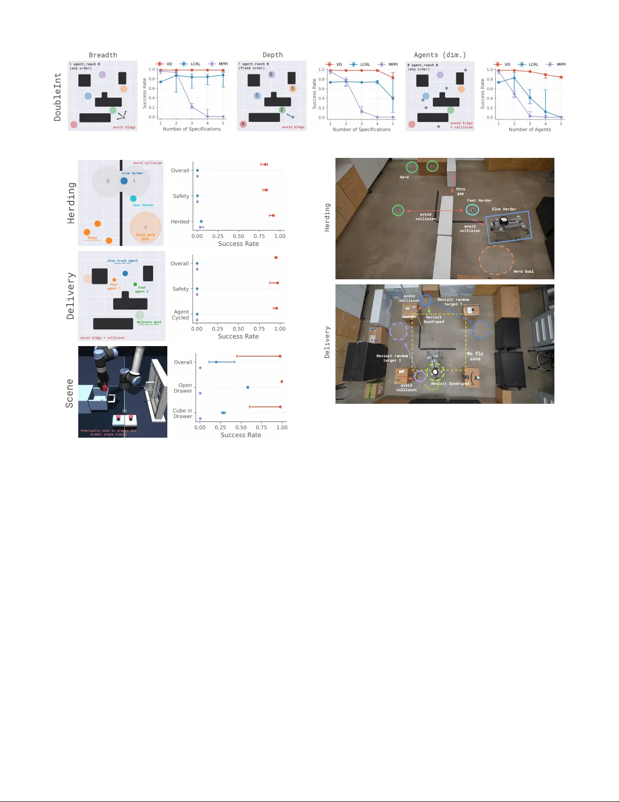
Bellman V alue Decomposition for T ask Logic in Safe Optimal Control W illiam Sharpless ∗ , 1 , Oswin So ∗ , 2 , Dylan Hirsch 1 , Sylvia Herbert 1 , Chuchu Fan 2 1 UCSD, 2 MIT , ∗ Equal contribution, wsharpless@ucsd.edu Fig. 1: V alue-Decomposition and VDPPO. The Bellman V alue for a range of temporal logic (e.g., multi-goal, recurrence, stability , safety) decomposes into a V alue graph connected by atomic Bellman equations (Thms. 1–4). W e propose VDPPO, an algorithm that exploits this structure to learn policies for complex, high-dimensional tasks. Our approach is validated on hardware with Herding and Delivery , two complex tasks inv olving a heterogeneous team of drones and a quadruped. I . A B S T R AC T Real-world tasks in volve nuanced combinations of goal and safety speciﬁcations. In high dimensions, the challenge is exacerbated: formal automata become cumbersome, and the combination of sparse re wards tends to require laborious tuning. In this work, we consider the innate structure of the Bellman V alue as a means to naturally or ganize the problem for improv ed automatic performance. Namely , we pro ve the Bellman V alue for a complex task deﬁned in temporal logic can be decomposed into a graph of Bellman V alues , connected by a set of well-known Bellman equations (BEs): the Reach-A void BE, the A void BE, and a novel type, the Reach-A void-Loop BE. T o solve the V alue and optimal policy , we propose VDPPO , which embeds the decomposed V alue graph into a two-layer neural net , bootstrapping the implicit dependencies. W e conduct a variety of simulated and hardware experiments to test our method on complex, high-dimensional tasks in volving heterogeneous teams and nonlinear dynamics. Ultimately , we ﬁnd this approach greatly improves performance o ver existing baselines, balancing safety and liveness automatically . I I . I N T RO D U C T I O N A N D R E L A T E D W O R K Reinforcement Learning (RL) typically optimizes e xpected cumulati ve rew ard [ 1 ], making it ill-suited for safety-critical or temporally structured tasks that require worst-case guarantees or satisfaction at speciﬁc times. Such objectives are naturally expressed using T emporal Logic (TL) [ 2 ], but TL itself does not prescribe how to act. Existing RL–TL methods therefore face a trade-of f between sparse binary rewards that slow learning and hand-crafted dense rewards that can misalign objecti ves. Hamilton–Jacobi Reachability (HJR) [ 3 , 4 ] provides optimal controllers for basic safety and liveness tasks via max–min Bellman equations, yielding dense and informative learning signals. Recent work sho wed that certain TL tasks can be solv ed e xactly by decomposing their v alue functions into sequences of simple HJR problems [ 5 ]. W e generalize this idea to a broad class of TL speciﬁcations, introduce a value-function decomposition algebra and a corresponding PPO variant, and demonstrate ef fectiv eness in simulation and real-world drone and quadruped experiments. RL with TL speciﬁcations A large body of work study RL with TL speciﬁcations [ 6 , 7 , 8 , 9 , 10 , 11 ], including approaches based on Non-Markovian Reward Decision Processes [ 12 , 13 , 14 , 15 , 2 ], approximated quantitati ve semantics [ 16 , 17 , 18 ], modiﬁed Bellman equations [ 19 , 20 , 21 ], or multiple discounted rew ards [ 22 , 23 , 24 ]. In contrast, our method exactly decom- poses TL value functions into simpler objectiv es solved via HJR, av oiding semantic approximation and long-horizon re ward 1 sparsity . Additional discussion appears in the Appendix and [ 5 ]. Constrained, Multi-Objective, and Goal-Conditioned RL. Constrained MDPs (CMDPs) maximize discounted rewards subject to constraints, typically via Lagrangian relaxation [ 25 , 26 , 27 , 28 , 29 , 30 , 31 , 32 , 33 , 34 , 35 , 36 , 37 , 38 ], but require careful tuning and are ill-suited to general TL objectiv es. Multi-objectiv e RL instead Pareto-optimizes multiple reward sums [ 39 , 40 , 41 , 42 , 43 , 44 , 45 ], yet does not naturally encode TL structure. Goal-conditioned RL learns policies over a family of goals [ 46 , 47 , 48 , 49 , 50 , 51 , 52 , 49 , 50 , 53 ], but dif fers fundamentally from TL settings, where all speciﬁcations must be jointly satisﬁed. Hamilton–Jacobi Reachability . HJR was originally devel- oped to compute value functions for reach, av oid, and reach- av oid problems in continuous time and space [ 3 , 4 ], correspond- ing to the quantitativ e semantics of ev entually , always, and until predicates [ 54 ]. Recent work has successfully integrated HJR into RL framew orks [ 55 , 56 , 57 , 58 , 59 , 60 ]. Our work builds on these results by decomposing value functions for complex TL objectiv es into sequences of simpler HJR problems. I I I . C O N T R I B U T I O N S 1) W e establish a formal connection between T emporal Logic and Bellman V alue theory , characterizing both equiv alences (Lem. 1) and div ergences (e.g., Rem. 1). 2) W e prov e that a broad class of TL predicates admits an exact decomposition of the V alue function into a directed graph of atomic Bellman equations (Thms. 1, 3, 4), including a nov el Reach–A void–Loop Bellman equation for always–e ventually speciﬁcations (Lem. 2). 3) W e introduce VDPPO , an algorithm that solves the decomposed value graph, and demonstrate its effecti veness through e xtensiv e simulation and real-world hardware experiments, achieving improved speed and success ov er existing methods. I V . P R E L I M I NA R I E S Giv en a discrete-time system x t +1 = f ( x t , a t ) with state x t ∈ X ⊆ R n and action a t ∈ A ⊆ R m , a trajectory beginning at x is a sequence of states ξ α x := ( x, ... ) ∈ X := X N arising from actions α = ( a, ... ) ∈ A := A N . W e let ξ x ( t ) and α ( t ) be the state and action at time t . T o specify desired properties of a trajectory , let an atomic predicate r : R n → { true , false } be deﬁned by a bounded predicate function r : R n → R , also known as a target or rew ard function in HJR or RL. Gi ven a trajectory and time ( ξ x , t ) , r is satisﬁed (written ( ξ x , t ) | = r ) iff r ( ξ x ( t )) ≥ 0 , and thus, r is employed to represent the arriv al of a trajectory at a goal or obstacle (deﬁned by the 0 -level-set of r ). T o represent complex tasks, TL deﬁnes a logic for modular composition of predicates [ 61 ]. Namely , predicates may be composed via negation ( ¬ ), conjunction/and ( ∧ ), the Until operator ( U ) and the ne xt operator ( X ). W ith these operations, one may also deﬁne disjunction/or ( ∨ ), ﬁnally/ev entually ( F ), and globally/always ( G ). W e give these operators via the robustness score ρ : R n → R [ 62 ] because this is the payof f used in the corresponding HJB optimal control problem [ 3 , 4 ]. See the Appendix for more details. Deﬁnition 1. F or any pr edicate p composed of atomic pr edicates r i , let the r obustness scor e ρ [ p ] : X × N → R be deﬁned inductively with ρ [ r i ]( ξ x , t ) := r i ( ξ x ( t )) ρ [ ¬ p ]( ξ x , t ) := − ρ [ p ]( ξ x , t ) ρ [ p ∧ p ′ ]( ξ x , t ) := min  ρ [ p ]( ξ x , t ) , ρ [ p ′ ]( ξ x , t )  ρ [ p ∨ p ′ ]( ξ x , t ) := max  ρ [ p ]( ξ x , t ) , ρ [ p ′ ]( ξ x , t )  ρ [ Xp ]( ξ x , t ) := ρ [ p ]( ξ x , t + 1) ρ [ Fp ]( ξ x , t ) := max τ ≥ t ρ [ p ]( ξ x , τ ) ρ [ Gp ]( ξ x , t ) := min τ ≥ t ρ [ p ]( ξ x , τ ) ρ [ p U p ′ ]( ξ x , t ) := max τ ≥ t min  ρ [ p ′ ]( ξ x , τ ) , min κ ∈ [ t,τ ] ρ [ p ]( ξ x , κ )  with ( ξ x , t ) | = p ⇐ ⇒ ρ [ p ]( ξ x , t ) ≥ 0 . Note that Fp = ⊤ U p , where ⊤ is true, and thus it often sufﬁces to consider only the U and G in analysis. Similarly , Gq ∧ Gq ′ = G ( q ∧ q ′ ) = Gq ′′ so we write always speciﬁcations succintly . With this syntax, one may express the satisfaction of complex speciﬁcations over trajectories formally and succinctly . V . P RO B L E M F O R M U L A T I O N In this work, we consider the problem of synthesizing optimal actions α and a policy π : X → A (Appendix), such that for any initial state x the resulting trajectory ξ α x maximizes the payoff ρ for a giv en predicate. W e assume the system begins at t = 0 and evolv es indeﬁnitely . For brevity , we let ρ [ p ]( ξ ) := ρ [ p ]( ξ , 0) . This leads to the following inﬁnite-horizon Safe Optimal Control Problem (SOCP), maximize α ρ [ p ]( ξ α x ) , s.t. ξ α x ( t + 1) = f ( ξ α x ( t ) , α ( t )) . Note, because ρ is deﬁned by temporal extrema ( max / min ov er time), this program induces behavior characterized by its outlying performance , in contrast with a sum-based SOCP (in canonical RL [ 1 ]) which selects for average behavior . This objecti ve is explicitly captured by the Bellman V alue function, the “high score” function for the gi ven SOCP . Deﬁnition 2. F or a pr edicate p , we aim to solve the Bellman V alue function V ∗ [ p ]( x ) := max α ρ [ p ]( ξ α x ) . (1) W e hav e deﬁned the Bellman V alue for a general TL predicate p , or V ∗ p for brevity , but in fact, for the operations Gq and q U r this object has been extensiv ely studied in the HJR literature [ 3 , 57 , 63 ]. Namely , the V alue for these operations are known as the A VO I D ( A ) and R E AC H - A VO I D ( RA ) V alues. 2 In this context, the following contractive Bellman operations for these extrema-based V alues hav e been derived [57]. Deﬁnition 3. The A and RA Bellman operators [ 57 ], B γ A [ V ] := (1 − γ ) q + γ min { V + , q } , B γ RA [ V ] := (1 − γ ) min { r, q } + γ min { max { V + , r } , q } , wher e V + ( x ) := max a V ( f ( x, a )) , are contractive. F or V ∗ [ Gq ] and V ∗ [ q U r ] deﬁned in (1) , the ﬁxed points V γ [ Gq ] = B γ A [ V γ [ Gq ]] , V γ [ q U r ] = B γ RA [ V γ [ q U r ]] , satisfy lim γ → 1 V γ = V ∗ by Thm. 1 of [57]. These Bellman operators differ from those which arise with a discounted-sum [ 1 ], as they propagate maximum or minimum (extremum) values, thus encouraging behavior deﬁned by outlying performance. This has proved to make the RL algorithms based on these equations signiﬁcantly better at safety and achievement tasks [55, 64]. In a recent work [ 5 ], it was demonstrated that for simple conjunctions F r ∧ Gq and F r 1 ∧ F r 2 , one may decompose the corresponding Bellman V alues into these “atomic” BE, which in some ways resembles the base case for what follows. In this work, we generalize this principle, demonstrating that the A -BE and RA -BE, along with the novel R E A C H - A V O I D - L O O P BE (Lem. 2), serve as a set of “atomic” building blocks to decompose the Bellman V alue of complex TL predicates. V I . M OT I V A T I O N A. Why the V alue function? Abov e all, the V alue function serves to deﬁne an optimal policy for autonomy . Moreov er, this V alue function has se veral properties which motiv ate the work, and we discuss them here. V alue functions are stable, policies need not be. While the value function is Lipschitz continuous, its gradient—and thus the optimal polic y—may be discontinuous. Consequently , nearby states can induce very different optimal trajectories, making direct policy learning unstable under noise. The value remains inf ormative ev en for infeasible tasks. V ∗ p ( x ) characterizes both satisﬁability ( ≥ 0 ) and degree of violation. Hence, maximization produces policies that minimize failure when satisfaction is impossible. V alue decomposition yields dense, aligned lear ning signals. Sparse binary rewards provide little guidance, while dense re- wards under discounted sums often conﬂate with TL objectiv es. Decomposing the value function produces a hierarchy of dense re wards that directly reﬂect the structure of the TL speciﬁcation. Extremum-based decomposition enfor ces safety without tuning. Because each subproblem is governed by an extremum- based Bellman equation, worst-case and best-case outcomes propagate without additiv e trade-offs. This naturally prioritizes safety and goal achiev ement, avoiding the Lagrangian tuning required by constrained RL methods [28]. B. Optimality versus Satisfaction The decomposition of formal logic is well-studied in sev eral contexts, including formal veriﬁcation [ 65 ], automata theory [ 66 ], and temporal logic trees (TL T) [ 67 ]. This body of work has established a rich framework for understanding the structure and properties of temporal logic formulas, and has led to performant decompositional learning methods for complex tasks [ 68 ]. Howe ver , the algebra of TL, which is equi valent to the algebra ov er the robustness score, is fundamentally distinct from that of the V alue function due to the presence of the maximum over action sequences or control policies in (2) . This distinction is not only relev ant to theoretical analysis but can lead to safety failures and sub-optimality in real world applications. W e illustrate this with the following remark and offer concrete counter-examples in the Appendix. Remark 1. The following TL identity always holds: ρ [ F r ∧ Gq ]( ξ α x ) = min { ρ [ F r ]( ξ α x ) , ρ [ Gq ]( ξ α x ) } . By contrast, for the corresponding V alue, we have V ∗ [ F r ∧ Gq ]( x ) ≤ min { V ∗ [ F r ]( x ) , V ∗ [ Gq ]( x ) } , wher e the inequality is indeed strict when no single choice of action sequence can both reac h r and avoid ¬ q . V I I . R E S U L T S In this section, we present our main results regarding the decomposition of the Bellman V alue for complex TL predicates. W e begin by discussing the relationship between the V alue and TL algebra, and then proceed to present a series of decompo- sition theorems culminating in a general decomposition result for a class of TL predicates. In general, we seek to e xpress the Bellman V alue for a complex predicate in terms of simpler components that are themselves composed with the fundamental Bellman equations of HJR (and thus may be solv ed similarly), and we will observe that these are associated with subsets of the overall logic. W e give all proofs in the Appendix. A. Agr eeable Algebra W e begin by noting the similarity between the decomposition of the Bellman V alue and TL algebra. The presence of the max α in (1) does not always distinguish the V alue algebra from that of TL, namely when the TL is also deﬁned by maxima, as with ∨ and a “right-side” U (for which, F is a special case). The commutativity of max in this case yields a decomposition that mirrors that of the TL, gi ving the following results. Lemma 1. Let v p be the predicate for V [ p ] , i.e. ( ξ x , t ) | = v p ⇐ ⇒ V [ p ]( ξ x ( t )) ≥ 0 . Recall that ρ [ v p ]( ξ x , t ) := V [ p ]( ξ x ( t )) . (2) The following pr operties hold: 1) V [ a ∨ b ]( x ) = V [ v a ∨ v b ]( x ) 2) V [ a U b ]( x ) = V [ a U v b ]( x ) 3 Fig. 2: E.g. N -Until-Conjunction V alue Decomposition. Here we illustrate the primary decomposition result (Thm. 1 extension, Appendix), with a GridWorld example (left) for a given speciﬁcation. The corresponding DV G is shown (center left) with each node representing a decomposed V alue, and edges representing dependencies. In the center right, a subset of decomposed V alues solved with dynamic programming are shown, along with the discounted solution produced by VDPPO. On the right, the optimal path for a giv en initial condition is shown. This result makes some compositions of the V alue simple to consider . For example, we may know that the V alue for a series of Until predicates is equiv alent to a chain of Until V alues, i.e. a chain of RA V alues. Moreover , the V alue for F G , also known as the reach-stay problem, is simply a R V alue where the target is the A V alue associated with the always predicate. See the Appendix for more details. These results, howe ver , do not apply when the TL is deﬁned by min as with ∧ , and thus are insufﬁ- cient to decompose the V alue for many common TL predicates. B. N -Until-Conjunction Decomposition W e next present the ﬁrst major result of the work concerning the decomposition of the Bellman V alue for the conjunction of N Until predicates, or equiv alently , the N - RA V alue. This result is a generalization of the RR V alue function decomposition in [ 5 ], which explored the independent pairwise combination of two reach tasks. Theorem 1. F or the pr edicate p := V i ∈I ( q i U r i ) , the corr esponding Bellman V alue satisﬁes V ∗  ^ i ( q i U r i )  ( x ) = V ∗  ˜ q U ˜ r  ( x ) wher e, ˜ r := _ i  r i ∧ v ∗ p − i  , ˜ q := ^ i q i , and p − i := V j ∈I \{ i } q j U r j . This result giv es an equivalence between the N - RA V alue and the V alue function of a single RA task, which has abstract reach and avoid predicates in the sense that they no longer represent physical goals or obstacles. Instead, the new reach predicate ˜ r is deﬁned by the disjunction of N conjunctions that each correspond to reaching one of the predicates r i and being able to satisfy the remaining logic p − i , i.e. having V ∗ p − i > 0 . The ne w avoid predicate ˜ q is deﬁned by the conjunction of all N-av oid predicates and hence implies that we need to a void all q j . Intuitiv ely , Thm. 1 breaks down the optimal v alue for the conjunction of N Untils into the goal of reaching any of the predicates while being able to satisfy the rest of the predicate of N − 1 Until operations, denoted p − i , where r i has been ’popped off ’ the original predicate. Notably , Thm. 1 is recursive, and, therefore, we may reapply the result iteratively to the N - RA V alue to break it into N decomposable sub-V alues and so forth, giving 2 N − 1 V alues in total. Crucially , as each of these V alues is equiv alent to a special Until V alue, they may each be solved with the discounted RA -BE with their respectiv e rewards. W e demonstrate this result in Fig.2 with a simple GridWorld problem, where the true solution may be solved via dynamic programming. Analogous to the proof of the Reach-Always-A void V alue in [ 5 ], this result can in fact be extended to the case where p := V i ∈I ( q i U r i ) ∧ Gq . In this case, the only difference is that the presence of Gq persists to the ultimate sub-V alue, which is at this point equivalent to the RAA V alue posed in [5]. W e giv e this in the Appendix. C. Recursive Decompositions In this section, we consider the family of recurrence relation operations corresponding to the composition of G with U (for which GF is a special case). T o always-e ventually satisfy a predicate implies that a trajectory must continue to satisfy it indeﬁnitely . These compositions are particularly important as they encompass the liv eness property , arising in safety-critical applications where certain states or tasks must be revisited or regenerated in some sense. Moreov er, this operation is signiﬁcantly less strict than the F G (which requires that we ev entually satisfy the predicate continuously), and thus more desirable, when the possibility of satisfaction is unknown. The temporal coupling of the outer G with the inner TL makes the V alue of these compositions more challenging to characterize and decompose, and in general may not be unique . W e begin with a formal characterization of the V alue in this situation for the base-case predicate G ( q U r ) . 4 Fig. 3: E.g. G ( N -Until-Conjunction) V alue Decomposition. W e illustrate the recursive decomposition result (Thm. 3), with a GridWorld example (left) for a giv en speciﬁcation. The plots here are analogous to those of Fig. 2, with the D VG (center left), decomposed V alues (center right), and optimal path (right). Note, the optimal path for the discounted case differs due to the subtle effect of discounting the V alue associated with a G composition, which selects for shorter loops (Sec. VII-C). Theorem 2. F or the predicate p := G ( q U r ) the corr esponding Bellman V alue satisﬁes V ∗ [ G ( q U r )]( x ) = V ∗  q U ( r ∧ Xv ∗ p )]( x ) . This result demonstrates that the V alue function associated with the predicate G ( q U r ) can be characterized recursively . Intuitiv ely , one may consider this V alue as a special RA V alue that aims to reach an intersection of the target predicate r and its own satisﬁable set (denoted by v ∗ p ) at the next step, and hence, maintain the ability to satisfy it again in the future. More generally , we may expand this result to the case in volving a composition fo G with N -Until-Conjunctions, formalized in the following result. Theorem 3. Given the set of coupled Bellman V alues of length J = |J | , V ∗ j ( x ) := V ∗  ˜ q j U ( ˜ r j ∧ Xv ∗ j +1 )  ( x ) wher e J + 1 := 1 , ˜ q j := q j ∧ ( q j +1 ∨ r j +1 ) , and ˜ r j := r j ∧ ( q j +1 ∨ r j +1 ) , then ∀ j , deﬁned by V ∗   G   ^ j ∈J ( q j U r j )     ( x ) = V ∗ j ( x ) . This result allows us to consider the problem of recurrently reach-av oiding N tasks as a loop of N coupled RA ℓ V alues. Note, in this case, the ﬁxed iteration order is equiv alent to any ordering giv en in Thm. 1 because of the inﬁnite nature of the problem (see Appendix). Although, these results appear like the pre vious decompositions, it is important to note that they are fundamentally dif ferent due to the implicit deﬁnition of the V alue. These characterizations do not guarantee uniqueness or existence of the V alue, and in continuous state spaces, they may be ill-deﬁned. T o certify the existence in certain scenarios (e.g. ﬁnite state spaces), we show in the Appendix that these V alues are equiv alent to the limit of ﬁnite recurrence, howe ver , this is not generally a practical procedure. Moreov er, a straightforward application of the discounted RA -BE yields a BE that is not guaranteed to be contractive , due to the appearance of the V alue in both (1 − γ ) and γ terms. T o address these challenges, we propose a nov el contractiv e Bellman Equation, which we call the RA -Loop ( RA ℓ ) BE, which is guaranteed to solve the family of G ( ... ) predicates in the limit of discounting. Lemma 2. F or the set of J V alues deﬁned in Thm. 3, let the RA ℓ -BE be deﬁned as B γ RA ℓ [ V j ] := (1 − γ ) min { ˜ r j , ˜ q j } + γ min n max n min  ˜ r j , V + j +1  , V + j o , ˜ q j o . This is contr active such that V γ j = B γ RA ℓ [ V γ j ] has a unique ﬁxed point, satisfying lim γ → 1 V γ j = V ∗ [ G ( V j ∈J ( q j U r j ))] . Equipped with the RA ℓ -BE, we can now tackle the problem of computing the V alue function for the family of G ( ... ) predicates effecti vely . D. A general result for a class of predicates Here, we give the ﬁnal decompositional result of the paper , combining se veral of the pre vious results. Note, we present this as a culmination of the dif ferent algebraic decompositions of the V alue to certify the decomposition of a general class of TL predicates, including all of those inv olved in the work. Theorem 4. F or the predicate p := ^ i ∈I ( q i U r i ) ! ∧ G   ^ j ∈J ( q j U r j )   ∧ Gq 5 the corr esponding optimal V alue satisﬁes V ∗ [ p ]( x ) = V ∗  ˜ q U ˜ r  ( x ) wher e ˜ r := _ i  r i ∧ v ∗ p − i  , ˜ q := ^ k ∈I ×J ˜ q k ∧ q , p − i := ^ k ∈I \{ i } ( q k U r k ) ∧ G   ^ j ∈J ( q j U r j )   ∧ Gq . Akin to previous results, Thm. 4 demonstrates that the giv en predicate p , in v olving the conjunction of N -Until predicates and the composition of G with N -Until predicates, may be rewritten as a single RA V alue. The residual V alue of this decomposition is the V alue associated with the composition of G with N - Until predicates, and can thus be recursiv ely decomposed with Thm. 3. See the Appendix for the complete proof. V I I I . A L G O R I T H M ( S ) In this section, we introduce V alue-Decomposition PPO, a variant of PPO that solv es the Bellman value associated with the class of TL predicates in Sec. VII using the decomposed value graph (D VG). W e also describe the tools required to generate the D VG and to solve it via dynamic programming for low-dimensional problems. A graphical overvie w is sho wn in Fig. 4, and all relevant code is provided in the Appendix. valtr : Generating the DV G . W e introduce valtr , a tool that con verts a parsed temporal logic speciﬁcation into the general predicate form of Thm. 4 by recursi vely applying standard TL rules. This representation is then transformed into the directed ac yclic graph (D A G) of the D VG, where nodes correspond to predicates, negations, max , min , and value functions, and edges encode their dependencies. Cyclic G compositions are handled via a special node, enabling efﬁcient parsing and transformation of arbitrary predicates into DV Gs. See the Appendix for details. Dynamic Programming with the DV G. W ith the DV G, one may compute the V alue of a given predicate by performing a topological sort of the D A G and applying dynamic program- ming to compute the V alue of each subformula in the correct order . This allo ws us to compute the dynamic programming solution for the low-d test cases given in Figs. 2 and 3. VDPPO. Finally , we propose V alue-Decomposition PPO (VDPPO), a special v ariant of PPO which solves the Bellman V alue associated with the class of TL predicates in Sec. VII by using the DV G. In this method, we use a shared trunk for each decomposed V alue in the D VG by embedding the node representations with a one-hot vector . Depending on the embedding value, the trunk is trained with the corresponding discounted A -BE, RA -BE or RA ℓ -BE by using the appropriate BE to compute the advantage estimate. Note, by deﬁnition this requires boot-strapping the current V alue estimate for each node, which is represented by the feedback loop in Fig. 4. The policy also uses a shared trunk with the embedded v alue and is trained with the standard PPO objectiv e, using the advantage estimate corresponding Fig. 4: Graphical Depiction of Algorithms. to the embedding. This allows us to le verage the decomposed structure of the V alue functions to efﬁciently learn policies that satisfy complex TL speciﬁcations without sequentially approximating the V alue. See the Appendix for further details. I X . S I M U L A T I O N R E S U LT S T o better understand the performance of VDPPO, we design simulation experiments to answer the following questions: ( Q1): Does value decomposition help with satisfying more complex temporal logic speciﬁcations (in both breadth and depth)? ( Q2): Does value decomposition help with scaling to multiple agents? ( Q3): Can VDPPO scale to more comple x dynamics? Additional ablation studies are provided in the Appendix. A. Setup En vironments. W e ev aluate on four simulated domains: DoubleInt (toy double integrator en vironment to focus on TL challenges), Herding (a team of herders collaborates to herd multiple targets to a designated location while av oiding obstacles), Delivery (agents must continuously pick up and deliv er packages to a special agent while av oiding collisions with each other and static obstacles), and Manipulator (a robotic arm interacts with a cube and a dra wer as speciﬁed by TL formulas). Baselines. W e compare VDPPO with other model-free methods that can solve TL speciﬁcations with black-box dynamics. These include LCRL [ 69 ], a deep RL method that solves TL tasks by augmenting the state space with an automata representation of the TL formula, and an e xtension of Model Predictiv e Path Inte gral (MPPI) [ 70 ] to tackle TL problems [ 71 ], which we denote TL-MPPI. For each en vironment, LCRL and VDPPO are run for the same number of update steps, while for TL-MPPI we follow the hyperparameters chosen in [71]. Evaluation criteria. Performance is measured by success rate on ﬁnite-horizon TL satisfaction; we additionally report satisfaction rates of individual subformulas. All methods are trained with three seeds and ev aluated on 256 initial conditions. B. Results (Q1): V alue decomposition improves scalability with TL complexity . W e study two TL families of increasing complexity in a single-agent double-integrator environment. Breadth speciﬁcations combine a safety constraint with an increasing number of unordered Finally goals, while depth speciﬁcations contain nested Finally operators enforcing a ﬁxed order . Results are sho wn in Fig. 9. 6 Fig. 5: Performance scaling with TL complexity . V alue decomposition enables VDPPO to better scale by tackling smaller problems. Fig. 6: Complex high-dimensional tasks . VDPPO greatly outperforms baseline methods on more complex tasks. All methods solve the singular speciﬁcation b ut degrade as the number of speciﬁcations increases. VDPPO consistently outperforms both baselines as the complexity of the TL speciﬁ- cations increases in both breadth and depth, demonstrating the effecti veness of value decomposition in handling complex TL tasks. This is particularly true in the depth case, where both baselines achie ve ≤ 40% success rate for a depth of n = 5 . This is because the probability of satisfying nested TL speciﬁcations by luck decreases exponentially with depth, making it difﬁcult for non-decompositional methods to learn effectiv e policies. (Q2): V alue decomposition strongly helps with increasing number of agents. Compared to the Breadth plot where we only increase the number of speciﬁcations, we scale both the number of agents and the number of speciﬁcations simultane- ously and sho w the results in Fig. 9. Increasing the number of agents increases the action dimension, which increases the difﬁculty of exploration. This de grades the performance of all methods. Howe ver , VDPPO is least impacted by this and is the only method that solves the problem with 5 agents. (Q3): VDPPO shines on problems with difﬁcult dynamics. W e now consider more challenging problems, either due to Fig. 7: Hardware Overview for Herding and Delivery T asks complex interactions with uncontrolled agents ( Herding ), needing to collaborate ( Delivery ), or complex dynamics ( Manipulator ) and show the results in Fig. 6. In all three tasks, VDPPO achiev es the highest success rate by a signiﬁcant margin. See the Appendix for ablations. X . H A R DWA R E R E S U LT S Lastly , we perform hardware experiments corresponding to the Herding and Delivery en vironments using a swarm of Crazyﬂie (CF) drones collaborating with the Unitree Go2 to demonstrate the ability of VDPPO to solve complex task speciﬁcations in high-dimensional real-world settings with heterogeneous collaboration. See Fig. 7 for an overvie w . A. Herding In this experiment, we consider a team of one CF and the Go2 tasked with herding three “sheep” CFs through a narrow gap to a target location while av oiding obstacles and collisions. The sheep CFs hav e a ﬁxed nominal polic y , using the softmin to driv e them away from the nearest obstacle or agent, and thus will move only when approached. The TL speciﬁcation for the task is given by , p herding := G ( ¬ c ) ∧ F ( r 0 ∧ F r 1 ) ∧ F G ( r h ) , where c denotes collisions, r 0 the herd reaching the pre-gate region, r 1 passage through the gate, and r h arri val at the target. 7 Fig. 8: T rajectory snapshots from Herding and Delivery hardwar e tasks . W e show a long-exposure photo (left), and stills from independent times (right), with depictions corresponding to those of the ov erview in Fig. 7. This encodes a sequence of reach–avoid objectiv es followed by a reach–stabilize objective requiring indeﬁnite herding. The herders (CF and Go2) are initialized opposite the gap from the herd and have asymmetric dynamics, with the Go2 moving more slowly . T o satisfy the speciﬁcation, the herders must coordinate to pass through the gap, collect the herd, and guide it to the target while av oiding obstacles. W e train a VDPPO policy using the D VG and deploy it on hardware, where the agents adapt online to real-time state feedback. Ultimately , we observe that the CF and Go2 learn to divide the labor of the task such that the CF passes through the gap to gather the agents (Fig.8.B), while the Go2 waits to recei ve on the herding side (Fig.8.C). When the herd passes through the narrow gap, the Go2 initially moves out of the way (Fig.8.C) and then transitions to providing support, rapidly shifting position to block the Herd from distributing across the new space (Fig.8.E). This behavior is entirely emergent and demonstrates the wide-ranging ability of VDPPO to solve complex tasks automatically . B. Delivery In this experiment, we consider a team of two CFs and the Go2 tasked with recurrently visiting agent-speciﬁc target locations and recurrently revisiting the Go2 agent (to model package deli very and resupply), while avoiding building obstacles, collisions, and a “no ﬂy zone” (for the CFs). The TL speciﬁcation for the task is given by , p deliv ery := ^ i GF ( r i ) ∧ ^ i GF ( rs i ) ∧ G ¬ ac ∧ G ¬ ob ∧ G ¬ nf where the predicate r i captures CF i visiting target i , rs i captures CF i visiting the Go2 (resupplying), ac captures aerial collision, ob captures obstacle collision, and nf captures the no- ﬂy-zone (for the CFs only). Here, the task logic is dominated by GF , and hence is largely solved with the RA ℓ -BE. In this en vironment, the CF tar gets jump to a ne w random location after an agent has visited it, requiring a policy that is conditioned to various target locations. The real difﬁculty of this problem arises in the tightness of the layout; the obstacles conﬁne the Go2 to the central area where the CFs are not allowed to ﬂy (modeling a b usy intersection), yet they must visit one another to “resupply”. W e again implement VDPPO to learn a policy to solve the complex task and deploy it live. Ultimately , we observ e sophisticated coordination between the three agents to distribute the difﬁculty of the task evenly . Namely , as the CFs mov e around the outskirts of the arena, av oiding one another carefully but not too cautiously (Fig.8.L), the Go2 anticipates their mov ements, moving between each of the agents (Fig.8.G-I) to be in position to resupply them as close to their target as possible. This complex collaboration generated by VDPPO allows the agents to rapidly meet deliv eries and resupply without crashing at all. X I . C O N C L U S I O N In this work, we propose a novel approach to solving the Bellman V alue associated with complex temporal speciﬁcations via decomposition. Namely , we demonstrate that for a large class of TL predicates, the corresponding Bellman V alue may be decomposed into a graph of V alues connected by a set of “atomic” Bellman equations. With this perspective, we propose VDPPO that is shown to solve optimal policies in complex tasks well beyond existing methods. This work highlights a nov el and powerful approach to tackling complex task logic for real-world autonomy . 8 R E F E R E N C E S [1] R. S. Sutton and A. G. Barto, Reinforcement Learning: An Intr oduction . Cambridge, MA, USA: A Bradford Book, 2018. [2] A. Camacho, R. T oro Icarte, T . Q. Klassen, R. V alenzano, and S. A. McIlraith, “L TL and beyond: Formal languages for reward function speciﬁcation in reinforcement learning, ” in Pr oceedings of the T wenty-Eighth International Joint Confer ence on Artiﬁcial Intelligence . California: International Joint Conferences on Artiﬁcial Intelligence Organization, 1 Aug. 2019, pp. 6065–6073. [3] I. M. Mitchell, A. M. Bayen, and C. J. T omlin, “ A time-dependent hamilton-jacobi formulation of reachable sets for continuous dynamic games, ” IEEE T ransactions on automatic contr ol , vol. 50, no. 7, pp. 947–957, 2005. [4] J. F . Fisac, M. Chen, C. J. T omlin, and S. S. Sastry , “Reach-av oid problems with time-varying dynamics, targets and constraints, ” in Hybrid Systems: Computation and Contr ol . A CM, 2015. [5] W . Sharpless, D. Hirsch, S. T onkens, N. Shinde, and S. Herbert, “Dual-objectiv e reinforcement learning with nov el hamilton-jacobi-bellman formulations, ” arXiv pr eprint arXiv:2506.16016 , 2025. [6] M. H. Cohen, Z. Serlin, K. Leahy , and C. Belta, “T emporal logic guided safe model-based reinforcement learning: A hybrid systems approach, ” Nonlinear Anal. Hybrid Syst. , vol. 47, no. 101295, p. 101295, Feb. 2023. [7] W . Qiu, W . Mao, and H. Zhu, “Instructing goal- conditioned reinforcement learning agents with temporal logic objectives, ” Neural Inf Pr ocess Syst , vol. 36, pp. 39 147–39 175, 2023. [8] T . Brázdil, K. Chatterjee, M. Chmelík, V . F orejt, J. K ˇ retínský, M. Kwiatkowska, D. Parker , and M. Ujma, “V eriﬁcation of Markov decision processes using learning algorithms, ” arXiv [cs.LO] , 10 Feb. 2014. [9] N. Hamilton, P . K. Robinette, and T . T . Johnson, “T raining agents to satisfy timed and untimed signal temporal logic speciﬁcations with reinforcement learning, ” in Software Engineering and F ormal Methods , ser . Lecture notes in computer science. Cham: Springer International Publishing, 2022, pp. 190–206. [10] D. Sadigh, E. S. Kim, S. Coogan, S. S. Sastry , and S. A. Seshia, “ A learning based approach to control synthesis of Markov decision processes for linear temporal logic speciﬁcations, ” in 53rd IEEE Conference on Decision and Contr ol . IEEE, Dec. 2014, pp. 1091–1096. [11] A. K. Bozkurt, Y . W ang, M. M. Zavlanos, and M. Pajic, “Control synthesis from linear temporal logic speciﬁcations using model-free reinforcement learning, ” in 2020 IEEE International Confer ence on Robotics and Automation (ICRA) . IEEE, May 2020, p. 10349–10355. [12] F . Bacchus, C. Boutilier , and A. J. Grove, “Rewarding behaviors, ” in Pr oceedings of the National Confer ence on Artiﬁcial Intelligence. cs.toronto.edu, 4 Aug. 1996, pp. 1160–1167. [13] S. Thiebaux, C. Gretton, J. Slaney , D. Price, and F . Kabanza, “Decision-theoretic planning with non- Markovian rewards, ” J . Artif. Intell. Res. , vol. 25, pp. 17–74, 29 Jan. 2006. [14] A. Camacho, O. Chen, S. Sanner , and S. McIlraith, “Non- Markovian rewards expressed in L TL: Guiding search via rew ard shaping, ” Pr oceedings of the International Symposium on Combinatorial Sear ch , vol. 8, no. 1, pp. 159–160, 1 Sep. 2021. [15] R. T . Icarte, T . Q. Klassen, R. V alenzano, and S. A. McIlraith, “Using reward machines for high-level task speciﬁcation and decomposition in reinforcement learning, ” ICML , vol. 80, pp. 2112–2121, 3 Jul. 2018. [16] D. Aksaray , A. Jones, Z. K ong, M. Schwager , and C. Belta, “Q-learning for robust satisfaction of signal temporal logic speciﬁcations, ” in 2016 IEEE 55th Confer ence on Decision and Control (CDC) . IEEE, Dec. 2016, pp. 6565–6570. [17] X. Li, C.-I. V asile, and C. Belta, “Reinforcement learning with temporal logic re wards, ” in 2017 IEEE/RSJ International Conference on Intelligent Robots and Systems (IR OS) . IEEE, Sep. 2017, pp. 3834–3839. [18] M. Cai, M. Hasanbeig, S. Xiao, A. Abate, and Z. Kan, “Modular deep reinforcement learning for continuous motion planning with temporal logic, ” IEEE Robotics and Automation Letter s , vol. 6, no. 4, p. 7973–7980, Oct. 2021. [Online]. A vailable: http://dx.doi.org/10.1109/LRA.2021.3101544 [19] R. W ang, P . Zhong, S. S. Du, R. R. Salakhutdinov , and L. Y ang, “Planning with general objectiv e functions: Going beyond total rewards, ” in Advances in Neural Information Pr ocessing Systems , H. Larochelle, M. Ranzato, R. Hadsell, M. Balcan, and H. Lin, Eds., vol. 33. Curran Associates, Inc., 2020, pp. 14 486–14 497. [20] W . Cui and W . Y u, “Reinforcement learning with non-cumulativ e objectiv e, ” IEEE T ransactions on Machine Learning in Communications and Networking , vol. 1, pp. 124–137, 2023. [21] Y . T ang, Y . Zhang, J. Ackermann, Y .-J. Zhang, S. Nishi- mori, and M. Sugiyama, “Recursi ve reward aggregation, ” in Reinfor cement Learning Conference , 2025. [22] H. van Seijen, M. Fatemi, J. Romoff, R. Laroche, T . Barnes, and J. Tsang, “Hybrid rew ard architecture for reinforcement learning, ” in Pr oceedings of the 31st International Confer ence on Neural Information Pr ocessing Systems , ser . NIPS’17. Red Hook, NY , USA: Curran Associates Inc., 2017, p. 5398–5408. [23] S. Pitis, “Consistent aggregation of objectives with di verse time preferences requires non-markovian rewards, ” in Thirty-seventh Confer ence on Neural Information Pr ocessing Systems , 2023. [24] Z. Lin, D. Y ang, L. Zhao, T . Qin, G. Y ang, and T .-Y . Liu, “Rdˆ2: Re ward decomposition with representation decomposition, ” in Advances in Neural Information Pr ocessing Systems , H. Larochelle, M. Ranzato, R. Hadsell, M. Balcan, and H. Lin, Eds., vol. 33. Curran 9 Associates, Inc., 2020, pp. 11 298–11 308. [25] E. Altman, Constrained Markov decision pr ocesses: Stochastic modeling . Boca Raton: Routledge, 13 Dec. 2021. [26] J. Achiam, D. Held, A. T amar, and P . Abbeel, “Constrained polic y optimization, ” ICML , v ol. abs/1705.10528, pp. 22–31, 30 May 2017. [27] A. W achi and Y . Sui, “Safe reinforcement learning in constrained Markov decision processes, ” ICML , vol. 119, pp. 9797–9806, 12 Jul. 2020. [28] A. Stooke, J. Achiam, and P . Abbeel, “Responsi ve safety in reinforcement learning by PID lagrangian methods, ” ICML , vol. 119, pp. 9133–9143, 8 Jul. 2020. [29] T . Li, Z. Guan, S. Zou, T . Xu, Y . Liang, and G. Lan, “Faster algorithm and sharper analysis for constrained Markov decision process, ” Oper . Res. Lett. , vol. 54, no. 107107, p. 107107, May 2024. [30] Y . Chen, J. Dong, and Z. W ang, “ A primal-dual approach to constrained Mark ov decision processes, ” arXiv [math.OC] , 26 Jan. 2021. [31] S. Miryooseﬁ and C. Jin, “ A simple rew ard-free approach to constrained reinforcement learning, ” ICML , v ol. abs/2107.05216, pp. 15 666–15 698, 12 Jul. 2021. [32] T .-Y . Y ang, J. Rosca, K. Narasimhan, and P . J. Ramadge, “Projection-based constrained polic y optimization, ” arXiv [cs.LG] , 7 Oct. 2020. [33] D. Ding, K. Zhang, T . Ba ¸ sar , and M. Jov anovi ´ c, “Natural policy gradient primal-dual method for constrained Markov decision processes, ” Neural Inf Process Syst , vol. 33, pp. 8378–8390, 2020. [34] C. T essler, D. J. Manko witz, and S. Mannor, “Reward constrained policy optimization, ” arXiv [cs.LG] , 28 May 2018. [35] A. Gattami, Q. Bai, and V . Aggarwal, “Reinforcement learning for constrained Markov decision processes, ” AIST A TS , vol. 130, pp. 2656–2664, 2021. [36] H. Satija, P . Amortila, and J. Pineau, “Constrained Marko v decision processes via backward value functions, ” ICML , vol. 119, pp. 8502–8511, 12 Jul. 2020. [37] A. Castellano, H. Min, E. Mallada, and J. A. Bazerque, “Reinforcement learning with almost sure constraints, ” in Pr oceedings of The 4th Annual Learning for Dynamics and Control Confer ence , ser . Proceedings of Machine Learning Research, vol. 168. PMLR, 2022, pp. 559–570. [38] J. McMahan and X. Zhu, “ Anytime-constrained reinforcement learning, ” in Proceedings of The 27th International Confer ence on Artiﬁcial Intelligence and Statistics , ser . Proceedings of Machine Learning Research, S. Dasgupta, S. Mandt, and Y . Li, Eds., vol. 238. PMLR, 02–04 May 2024, pp. 4321–4329. [39] M. A. Wiering, M. W ithagen, and M. M. Drugan, “Model-based multi-objective reinforcement learning, ” in 2014 IEEE Symposium on Adaptive Dynamic Pr ogramming and Reinfor cement Learning (ADPRL) . IEEE, Dec. 2014, pp. 1–6. [40] M. K. V an and A. Nowé, “Multi-objecti ve reinforcement learning using sets of Pareto dominating policies, ” The Journal of Machine Learning Resear ch , vol. 15, no. 1, pp. 3483–3512, 2014. [41] X.-Q. Cai, P . Zhang, L. Zhao, J. Bian, M. Sugiyama, and A. Llorens, “Distributional Pareto-optimal multi-objectiv e reinforcement learning, ” Neural Inf Pr ocess Syst , vol. 36, pp. 15 593–15 613, 2023. [42] H. Mossalam, Y . M. Assael, D. M. Roijers, and S. Whiteson, “Multi-objective deep reinforcement learning, ” arXiv [cs.AI] , 9 Oct. 2016. [43] A. Abels, D. Roijers, T . Lenaerts, A. Nowé, and D. Steck- elmacher , “Dynamic weights in multi-objectiv e deep reinforcement learning, ” in Pr oceedings of the 36th Inter- national Confer ence on Machine Learning , ser . Proceed- ings of Machine Learning Research, K. Chaudhuri and R. Salakhutdinov , Eds., vol. 97. PMLR, 2019, pp. 11–20. [44] R. Y ang, X. Sun, and K. Narasimhan, “ A generalized algorithm for multi-objective reinforcement learning and policy adaptation, ” in Advances in Neural Information Pr ocessing Systems . proceedings.neurips.cc, 2019. [45] E. Liu, Y .-C. W u, X. Huang, C. Gao, R.-J. W ang, K. Xue, and C. Qian, “Pareto set learning for multi-objecti ve rein- forcement learning, ” Pr oceedings of the AAAI Confer ence on Artiﬁcial Intelligence , vol. 39, no. 18, 2025. [46] M. Liu, M. Zhu, and W . Zhang, “Goal-conditioned reinforcement learning: Problems and solutions, ” arXiv [cs.AI] , 20 Jan. 2022. [47] M. Plappert, M. Andrychowicz, A. Ray , B. McGrew , B. Baker , G. Powell, J. Schneider, J. T obin, M. Chociej, P . W elinder , V . Kumar , and W . Zaremba, “Multi-goal re- inforcement learning: Challenging robotics en vironments and request for research, ” arXiv [cs.LG] , 26 Feb. 2018. [48] Z. Ren, K. Dong, Y . Zhou, Q. Liu, and J. Peng, “Exploration via hindsight goal generation, ” Neural Inf Pr ocess Syst , vol. 32, pp. 13 464–13 474, 1 Jun. 2019. [49] J. Y . Ma, J. Y an, D. Jayaraman, and O. Bastani, “Ofﬂine goal-conditioned reinforcement learning via f- adv antage regression, ” in Advances in Neural Information Pr ocessing Systems , S. Ko yejo, S. Mohamed, A. Agarwal, D. Belgrav e, K. Cho, and A. Oh, Eds., v ol. 35. Curran Associates, Inc., 2022, pp. 310–323. [50] A. Campero, R. Raileanu, H. Küttler, J. B. T enenbaum, T . Rocktäschel, and E. Grefenstette, “Learning with AMIGo: Adversarially motiv ated intrinsic goals, ” arXiv [cs.LG] , 22 Jun. 2020. [51] A. R. Trott, S. Zheng, C. Xiong, and R. Socher, “Keeping your distance: Solving sparse reward tasks using self-balancing shaped re wards, ” Neural Inf Pr ocess Syst , vol. abs/1911.01417, 4 No v . 2019. [52] B. Eysenbach, T . Zhang, R. Salakhutdinov , and S. Levine, “Contrastiv e learning as goal-conditioned reinforcement learning, ” Neural Inf Pr ocess Syst , vol. abs/2206.07568, pp. 35 603–35 620, 15 Jun. 2022. [53] E. Chane-Sane, C. Schmid, and I. Laptev , “Goal- conditioned reinforcement learning with imagined subgoals, ” ICML , vol. abs/2107.00541, pp. 1430–1440, 10 1 Jul. 2021. [54] M. Chen, Q. T am, S. C. Livingston, and M. Pav one, “Sig- nal temporal logic meets reachability: Connections and ap- plications, ” in International W orkshop on the Algorithmic F oundations of Robotics . Springer , 2018, pp. 581–601. [55] O. So, C. Ge, and C. Fan, “Solving minimum-cost reach avoid using reinforcement learning, ” in The Thirty-eighth Annual Confer ence on Neural Information Pr ocessing Systems , 2024. [Online]. A vailable: https://openrevie w .net/forum?id=jzngdJQ2lY [56] K.-C. Hsu, V . Rubies-Royo, C. J. T omlin, and J. F . Fisac, “Safety and liv eness guarantees through reach-av oid reinforcement learning, ” in Pr oceedings of Robotics: Science and Systems , Held V irtually , July 2021. [57] J. F . Fisac, N. F . Lugov oy , V . Rubies-Royo, S. Ghosh, and C. J. T omlin, “Bridging hamilton-jacobi safety analysis and reinforcement learning, ” in 2019 International Confer ence on Robotics and Automation (ICRA) . IEEE, 2019, pp. 8550–8556. [58] M. Ganai, C. Hirayama, Y .-C. Chang, and S. Gao, “Learn- ing stabilization control from observations by learning lyapunov-like proxy models, ” 2023 IEEE International Confer ence on Robotics and A utomation (ICRA) , 2023. [59] D. Y u, H. Ma, S. Li, and J. Chen, “Reachability constrained reinforcement learning, ” in International Confer ence on Machine Learning . PMLR, 2022, pp. 25 636–25 655. [60] K. Zhu, F . Lan, W . Zhao, and T . Zhang, “Safe multi-agent reinforcement learning via approximate hamilton-jacobi reachability , ” J. Intell. Robot. Syst. , vol. 111, no. 1, 30 Dec. 2024. [61] O. Maler and D. Nick ovic, “Monitoring temporal properties of continuous signals, ” in International symposium on formal techniques in real-time and fault-tolerant systems . Springer , 2004, pp. 152–166. [62] A. Donzé and O. Maler , “Rob ust satisfaction of temporal logic over real-v alued signals, ” in International confer ence on formal modeling and analysis of timed systems . Springer , 2010, pp. 92–106. [63] S. Bansal, M. Chen, S. Herbert, and C. J. T omlin, “Hamilton-jacobi reachability: A brief o vervie w and recent adv ances, ” in 2017 IEEE 56th Annual Conference on De- cision and Contr ol (CDC) . IEEE, 2017, pp. 2242–2253. [64] M. Ganai, Z. Gong, C. Y u, S. Herbert, and S. Gao, “Iterativ e reachability estimation for safe reinforcement learning, ” Advances in Neural Information Pr ocessing Systems , vol. 36, pp. 69 764–69 797, 2023. [65] C. Baier and J.-P . Katoen, Principles of model c hecking . MIT press, 2008. [66] O. Grumberg, E. Clarke, and D. Peled, “Model checking, ” in International Confer ence on F oundations of Softwar e T echnology and Theoretical Computer Science; Springer: Berlin/Heidelber g, Germany , 1999. [67] G. Bombara, C.-I. V asile, F . Penedo, H. Y asuoka, and C. Belta, “ A decision tree approach to data classiﬁcation using signal temporal logic, ” in Pr oceedings of the 19th International Confer ence on Hybrid Systems: Computation and Contr ol , 2016, pp. 1–10. [68] Y . Meng, F . Chen, and C. Fan, “Tgpo: T emporal grounded policy optimization for signal temporal logic tasks, ” arXiv preprint , 2025. [69] M. Hasanbeig, D. Kroening, and A. Abate, “Lcrl: Certiﬁed policy synthesis via logically-constrained reinforcement learning, ” in International Confer ence on Quantitative Evaluation of SysT ems . Springer , 2022, pp. 217–231. [70] G. W illiams, P . Drews, B. Goldfain, J. M. Rehg, and E. A. Theodorou, “ Aggressi ve driving with model predictiv e path integral control, ” in 2016 IEEE international confer ence on r obotics and automation (ICRA) . IEEE, 2016, pp. 1433–1440. [71] P . Halder, H. Hombur ger , L. Kiltz, J. Reuter , and M. Althoff, “T rajectory planning with signal temporal logic costs using deterministic path integral optimization, ” arXiv pr eprint arXiv:2503.01476 , 2025. [72] L. Y ifru and A. Baheri, “Concurrent learning of control policy and unknown safety speciﬁcations in reinforcement learning, ” IEEE Open Journal of Contr ol Systems , vol. 3, pp. 266–281, 2024. [73] D. Kasenberg and M. Scheutz, “Interpretable apprenticeship learning with temporal logic speciﬁcations, ” in 2017 IEEE 56th Annual Conference on Decision and Contr ol (CDC) , 2017, pp. 4914–4921. [74] M. Gaon and R. Brafman, “Reinforcement learning with non-markovian rew ards, ” Pr oceedings of the AAAI Confer ence on Artiﬁcial Intelligence , vol. 34, no. 04, pp. 3980–3987, Apr . 2020. [75] K. Jothimurugan, S. Bansal, O. Bastani, and R. Alur , “Compositional reinforcement learning from logical speciﬁcations, ” in Advances in Neural Information Pr ocessing Systems , M. Ranzato, A. Beygelzimer , Y . Dauphin, P . Liang, and J. W . V aughan, Eds., vol. 34. Curran Associates, Inc., 2021, pp. 10 026–10 039. [76] A. Duret-Lutz, E. Renault, M. Colange, F . Renkin, A. Gbaguidi Aisse, P . Schlehuber-Caissier , T . Medioni, A. Martin, J. Dubois, C. Gillard et al. , “From spot 2.0 to spot 2.10: What’ s ne w?” in International Conference on Computer Aided V eriﬁcation . Springer , 2022, pp. 174–187. [77] R. Diestel, Graph theory . Springer Nature, 2025. [78] W . Rudin, “Principles of mathematical analysis, ” 3r d ed. , 1976. [79] J. Schulman, P . Moritz, S. Levine, M. Jordan, and P . Abbeel, “High-dimensional continuous control using generalized adv antage estimation, ” arXiv pr eprint arXiv:1506.02438 , 2015. [80] S. Park, K. Frans, B. Eysenbach, and S. Levine, “Ogbench: Benchmarking ofﬂine goal-conditioned rl, ” in International Confer ence on Learning Repr esentations (ICLR) , 2025. 11 A P P E N D I X C O N T E N T S A M O R E R E L A T E D W O R K S 13 B T E M P O R A L L O G I C 13 C L O G I C V S . V A L U E E X A M P L E S 17 D A G R E E A B L E A L G E B R A 18 E N - RA R E S U LT S 20 F N - RA ℓ R E S U L T S 21 G G ( . . . ) F I X E D P O I N T I T E R AT I O N 23 H G E N E R A L R E S U LT 29 I P O L I C Y R E S U LT S 29 J V A L T R D E TA I L S 34 K V D P P O D E TA I L S 34 L E N V I RO N M E N T S 34 M B A S E L I N E S 35 N A B L A T I O N S 35 O H A R DWA R E 35 U S E F U L P RO P E RT I E S A N D N OTA T I O N W e giv e here properties and notations for simplifying the following proofs. For a giv en action sequence α , α := ( a 1 , a 2 , . . . ) ∈ A := A N let a portion beginning at i and ending at j be written α i : j := ( a i , . . . a j ) . Moreov er , for a trajectory ξ α x , ξ α x := ( x, x 1 , . . . ) ∈ X := X N , where x i +1 = f ( x i , α i ) , it follows then that for α di vided into α t − := α 1: t & α t + := α t +1: ∞ , ξ α x = ξ α t + y , where y = ξ α t − x ( t ) . W e then hav e the following result corresponding to the decomposition of a controlled trajectory , which will be used ubiquitously . Lemma 3. Let X s.t. |X | < ∞ . Then for t ∈ N , α ∈ A , ξ α x ∈ X , and, x ∈ X , max α max t f ( ξ α x , t ) = max t max α t − max α t + f ( ξ α t + ξ α t − x ( t ) , t ) . 12 A . M O R E R E L A T E D W O R K S W e here giv e a slightly more expanded description of the related works compared to the main text. W e refer the reader to [5] for additional discussion of many of these works. Reinfor cement Learning with TL Objectiv es. Many works have explored ways to optimize objecti ves that encode TL speciﬁcations [ 6 , 7 , 8 , 9 , 10 , 11 , 72 ] (or conv ersely learn TL speciﬁcations from agent behavior [ 73 ]). One line of such works uses Non-Markovian-Re ward Decision Processes (NMRDPs), which allow for history-dependent rewards [ 2 , 13 , 14 , 15 , 74 ]. Other works optimize the quantitative semantics associated with an STL objectiv e, approximating the maximums and minimums in a sum-of-discounted rewards fashion, which are then solved with traditional methods [ 16 , 17 ], or otherwise encoding TL objectiv es through expectations [ 18 ]. Se veral other methods also exist that attempt to optimize general objecti ve functions using non-traditional Bellman equations [19, 20, 21] or handle discounted sums of multiple rewards or penalties [22, 23, 24]. W e also refer the reader to [ 75 ] for an approach that proceeds by composing learned sub-tasks into higher level ones using an additional planning algorithms rather than breaking a high-le vel task do wn into subtasks. By contrast to most of these previous approaches, our approach proceeds by decomposition of a TL-speciﬁed problem in an exact manner . Speciﬁcally , we decompose the value function associated with a quantitativ e semantic for a TL predicate into value functions associated with simpler objectiv es. These simpler objectives are then solv ed by le veraging powerful recent Hamilton-Jacobi Reachability (HJR) methods. (Note that these decompositions of the value functions are fundamentally different from decompositions of the quantitativ e semantics themselves.) This approach allows one to avoid approximations of the objective function or issues associated with sparsity of long-horizon rewards, which commonly afﬂict the previous methods. Constrained, Multi-Objective, and Goal-Conditioned RL A number of techniques in RL have arisen to handle constraints or multiple goals. Constrained MDPs (CMDPs) attempt to maximize sums of discounted rewards subject to a safety or liv eness condition, which is often handled via a Lagrangian term in the objectiv e function [ 25 , 26 , 27 , 28 , 29 , 30 , 31 , 32 , 33 , 34 , 35 , 36 , 37 , 38 ]. For CMDPs, the Lagrangian term inv olved typically requires substantial tuning for desired beha vior , severly limiting its use for satisfying general TL tasks. Multi-objective RL techniques, by contrast Pareto-optimize multiple sums of discounted rewards [ 39 , 40 , 41 , 42 , 43 , 44 , 45 ]. This allows users to balance multiple objectives, but generally are not built for handling TL-like speciﬁcations. Goal-conditioned RL, by contrast, simultaneously learns policies for a range of possible task speciﬁcations [ 46 , 47 , 48 , 49 , 50 , 51 , 52 , 49 , 50 , 53 ]. At the time of deployment, a user can then decide which speciﬁcation is most appropriate. This is fundamentally different from TL tasks, where all speciﬁcations must be satisﬁed. Hamilton-Jacobi Reachability Hamilton-Jacobi Reachability (HJR) methods were initially designed to solve value functions associated with "reach", "avoid", or "reach-avoid" problems using traditional dynamic programming for continuous space and times [ 3 , 4 ]. The objectiv es for these tasks are precisely the quantitativ e semantics for ev entually , nev er , and until predicates. HJR approaches hav e recently been adapted to solve these same problems in RL settings, with exciting performance [ 55 , 56 , 57 , 58 , 59 , 60 ]. Our work builds on such advancements, using the RL algorithms de veloped by these building blocks to accomplish higher-le vel tasks. B . T E M P O R A L L O G I C In this section, we giv e further background on the temporal logic used in the main text. W e begin with the logical deﬁnitions of the operators ∨ , ∧ , ¬ , X , F , G , U , alternatively deﬁned by their rob ustness metric in the main text. Deﬁnition 4. Let p , p ′ be pr edicates, ξ x ∈ X a trajectory be ginning at x ∈ X , and t ∈ N a starting time. The relation ( ξ x , t ) | = p is deﬁned as follows, ( ξ x , t ) | = r i ⇐ ⇒ r i ( ξ x ( t )) ≥ 0 , ( ξ x , t ) | = ¬ p ⇐ ⇒ ( ξ x , t ) | = p , ( ξ x , t ) | = p ∧ p ′ ⇐ ⇒ ( ξ x , t ) | = p and ( ξ x , t ) | = p ′ , ( ξ x , t ) | = p ∨ p ′ ⇐ ⇒ ( ξ x , t ) | = p or ( ξ x , t ) | = p ′ , ( ξ x , t ) | = Xp ⇐ ⇒ ( ξ x , t + 1) | = p , ( ξ x , t ) | = Fp ⇐ ⇒ ∃ τ ≥ t s.t. ( ξ x , τ ) | = p , ( ξ x , t ) | = Gp ⇐ ⇒ ∀ τ ≥ t, ( ξ x , τ ) | = p , ( ξ x , t ) | = p U p ′ ⇐ ⇒ ∃ τ ≥ t s.t. ( ξ x , τ ) | = p ′ and ∀ κ ∈ [ t, τ ] , ( ξ x , κ ) | = p . From these deﬁnitions, we may certify a few equi valence relations for rearranging certain combinations of operators, which will later prove to be useful. Note, for the interested reader all of the following equiv alences may be automatically veriﬁed with the tool Spot [76]. 13 Lemma 4. ( q 1 U r 1 ) ∧ ( q 2 U r 2 ) ≡ ( q 1 ∧ q 2 ) U  ( r 1 ∧ q 2 U r 2 ) ∨ ( r 2 ∧ q 1 U r 1 )  Pr oof. W e show this via double entailment. 1. LHS | = RHS: Suppose σ, 0 | = q 1 U r 1 ∧ q 2 U r 2 . Then, 1) Since σ, 0 | = q 1 U r 1 , there exists t 1 ≥ 0 such that σ , t 1 | = r 1 , and for all 0 ≤ k < t 1 , σ, k | = q 1 . 2) Since σ, 0 | = q 2 U r 2 , there exists t 2 ≥ 0 such that σ , t 2 | = r 2 , and for all 0 ≤ k < t 2 , σ, k | = q 2 . Let t = min( t 1 , t 2 ) . Since σ, k | = q 1 and σ, k | = q 2 for all 0 ≤ k < t , we have σ, k | = q 1 ∧ q 2 for all 0 ≤ k < t . W e now show that the goal is reached at time t . • ( t 1 ≤ t 2 ): Then, t = t 1 , and σ, t | = r 1 . Since t 2 ≥ t 1 and σ, k | = q 2 for all t ≤ k < t 2 , we hav e σ, t | = q 2 U r 2 . Hence, σ, t | = r 1 ∧ q 2 U r 2 . • ( t 2 < t 1 ): Then, t = t 2 , and σ, t | = r 2 . Since t 1 > t 2 and σ, k | = q 1 for all t ≤ k < t 1 , we hav e σ, t | = q 1 U r 1 . Hence, σ, t | = r 2 ∧ q 1 U r 1 . Thus, σ, 0 | = ( q 1 ∧ q 2 ) U  ( r 1 ∧ q 2 U r 2 ) ∨ ( r 2 ∧ q 1 U r 1 )  . 2. RHS | = LHS: Suppose σ, 0 | = ( q 1 ∧ q 2 ) U  ( r 1 ∧ q 2 U r 2 ) ∨ ( r 2 ∧ q 1 U r 1 )  . Then, there exists t ≥ 0 such that • σ, t | = ( r 1 ∧ q 2 U r 2 ) ∨ ( r 2 ∧ q 1 U r 1 ) • For all 0 ≤ k < t , σ, k | = q 1 ∧ q 2 . W e now split into two cases. 1) ( σ, t | = r 1 ∧ q 2 U r 2 ): • σ, t | = r 1 • Since σ, k | = q 1 for all 0 ≤ k < t , we have σ, 0 | = q 1 U r 1 . • There exists t 2 ≥ t such that σ , t 2 | = r 2 , and σ, k | = q 2 for all t ≤ k < t 2 . • Since σ, k | = q 2 for all 0 ≤ k < t 2 , we have σ, 0 | = q 2 U r 2 . • Thus, σ, 0 | = q 1 U r 1 ∧ q 2 U r 2 . 2) ( σ, t | = r 1 ∧ q 2 U r 2 ): The reasoning is symmetric to the previous case, yielding σ, 0 | = q 1 U r 1 ∧ q 2 U r 2 . Thus, σ, 0 | = q 1 U r 1 ∧ q 2 U r 2 . Since we have shown both directions, the equi valence holds. Lemma 5. p := n ^ i =1 ( q i U r i ) ≡  n ^ i =1 q i  U  n _ i =1  r i ∧ p − i   wher e p − i := V n j =1 ,j  = i ( q j U r j ) . Pr oof. W e prove this using induction on n . Base Case ( n = 2 ): This is e xactly the previous lemma 4. Inductiv e Step: Assume the statement holds for n = k , i.e., k ^ i =1 ( q i U r i ) ≡  k ^ i =1 q i  | {z } : = ˜ q U  k _ i =1  r i ∧ n ^ j =1 ,j  = i ( q j U r j )   | {z } : = ˜ r . 14 W e need to show it holds for n = k + 1 . k +1 ^ i =1 ( q i U r i ) =  k ^ i =1 ( q i U r i )  ∧ ( q k +1 U r k +1 ) ≡ ˜ q U ˜ r ∧ ( q k +1 U r k +1 ) ≡ ( ˜ q ∧ q k +1 ) U (( ˜ r ∧ q k +1 U r k +1 ) ∨ ( r k +1 ∧ ˜ q U ˜ r )) Note that ˜ q ∧ q k +1 = V k +1 i =1 q i . For the ﬁrst part, ˜ r ∧ q k +1 U r k +1 = k _ i =1  r i ∧ k ^ j =1 ,j  = i ( q j U r j )  ∧ q k +1 U r k +1 = k _ i =1  r i ∧ k ^ j =1 ,j  = i ( q j U r j ) ∧ q k +1 U r k +1  = k _ i =1  r i ∧ k +1 ^ j =1 ,j  = i ( q j U r j ) ∧ q k +1 U r k +1  . For the second part, r k +1 ∧ ˜ q U ˜ r = r k +1 ∧ k ^ i =1 ( q i U r i ) , = r k +1 ∧ k +1 ^ j =1 ,j  = k +1 ( q j U r j ) . Combining these two parts completes the inductive step: k +1 _ i =1  r i ∧ k +1 ^ j =1 ,j  = i ( q j U r j )  . Since the base case and inductive step hold, the statement holds for all n ≥ 2 . Corollary 1. p := n ^ i =1 ( q i U r i ) ∧ Gq ≡  n ^ i =1 q i ∧ q  U  n _ i =1  r i ∧ p − i   wher e p − i := V n j =1 ,j  = i ( q j U r j ) ∧ Gq . Pr oof. It sufﬁces to show that Gq = q U ˜ r where ˜ r = Gq . This follows directly from the deﬁnition of G and U , σ, 0 | = Gq ⇐ ⇒ ∀ t ≥ 0 , σ, t | = q ⇐ ⇒ ∃ t ′ ≥ 0 s.t. σ, t ′ | = Gq and ∀ 0 ≤ t < t ′ , σ, t | = q ⇐ ⇒ σ, 0 | = q U ˜ r . Additionally , we can show this kind of rearrangement for the GU composition as well, given by the follo wing result. Lemma 6. G ( q U r ) ≡ q U ( r ∧ XG ( q U r )) Pr oof. W e show this via double entailment. 1. (LHS | = RHS) Suppose σ, 0 | = G ( q U r ) . 15 • For all t ≥ 0 , there exists s t ≥ t such that σ, s t | = r and ∀ 0 ≤ t ′ < s t , σ, t ′ | = q . In particular, for t = 0 , there exists s 0 ≥ 0 such that σ , s 0 | = r . • Since G ( q U r ) is a tail property , we have σ, s 0 + 1 | = G ( q U r ) . • Thus, σ, s 0 | = r ∧ XG ( q U r ) . • Hence, σ, 0 | = q U ( r ∧ XG ( q U r )) . 2. (RHS | = LHS) Suppose σ, 0 | = q U ( r ∧ XG ( q U r )) . • By deﬁnition of U , there e xists t 0 ≥ 0 such that σ , t 0 | = r ∧ XG ( q U r ) s.t. ∀ 0 ≤ t < t 0 , σ, t | = q . • The conjunction implies that σ, t 0 + 1 | = G ( q U r ) . • Since G ( q U r ) is a tail property , this implies that σ , 0 | = G ( q U r ) . Since we have shown both directions, the equi valence holds. Next, we may extend this to the multi-Until case, in order to capture the behavior of multiple recurrent Until operators. Notably , in this case, the order does not matter, as all must be satisﬁed inﬁnitely often. This is formalized in the following result. Lemma 7. Given p := G  ( q 1 U r 1 ) ∧ ( q 2 U r 2 )  , it holds that p ≡ ˜ q 1 U  ˜ r 1 ∧  ˜ q 2 U ( ˜ r 2 ∧ p )   ≡ ˜ q 2 U  ˜ r 2 ∧  ˜ q 1 U ( ˜ r 1 ∧ p )   , wher e ˜ q i := q i ∧ ( q j ∨ r j ) , ˜ r i := r i ∧ ( q j ∨ r j ) . Pr oof. W e show this via double entailment. For brevity , let w 1 := ( q 1 ∨ r 1 ) , w 2 := ( q 2 ∨ r 2 ) . 1. (LHS | = RHS) Assume σ, 0 | = p . • For all t ≥ 0 , σ, t | = ( q 1 Ur 1 ) ∧ ( q 2 Ur 2 ) . Choose k 1 ≥ 0 with σ, k 1 | = r 1 and σ, t | = q 1 for t < k 1 . Then σ, t | = w 2 for t ≤ k 1 , so σ, t | = q 1 ∧ w 2 for t < k 1 . • From σ, k 1 | = q 2 Ur 2 , choose k 2 ≥ k 1 with σ, k 2 | = r 2 and σ, t | = q 2 for k 1 ≤ t < k 2 . Since p holds globally , σ, t | = w 1 on [ k 1 , k 2 ] and σ, k 2 | = p . Thus σ, k 1 | = ˜ q 2 U ( ˜ r 2 ∧ p ) , so σ, 0 satisﬁes the RHS. 2. (RHS | = LHS) Assume σ, 0 satisﬁes the RHS. • There exists k 1 ≥ 0 with σ, k 1 | = ˜ r 1 ∧ Ψ and σ, t | = q 1 ∧ w 2 for t < k 1 , where Ψ := ˜ q 2 U ( ˜ r 2 ∧ p ) . • From Ψ there exists k 2 ≥ k 1 with σ, k 2 | = ˜ r 2 ∧ p and σ, t | = q 2 ∧ w 1 for k 1 ≤ t < k 2 . Since σ, k 2 | = p , the property ( q 1 Ur 1 ) ∧ ( q 2 Ur 2 ) holds for all t ≥ k 2 . Using the witnesses k 1 and k 2 and the safety conditions above, it also holds for all t < k 2 . Hence σ, 0 | = p . Both directions hold, so the equivalence follows. W e now giv e a logical equiv alence for the general class of predicates considered in Thm. 4. Lemma 8. Consider the formula p I , J deﬁned as p I , J : = ^ i ∈I G ( q i U r i ) ∧ ^ j ∈J ( q j U r j ) ∧ Gq Then, p I , J can be equivalently written as a single nested until formula: p I , J ≡ ˜ q I , J U ˜ r I , J , 16 wher e ˜ q I , J : = ^ j ∈J q j ∧ q ∧ ^ i ∈I ( q i ∨ r i ) , ˜ r I , J : = _ j ∈J r j ∧ Φ I , J \{ j } and p I , ∅ ≡ G  ^ i ∈I  q i ∧ q  U  r i ∧ q   . Pr oof. W e start by proving p I , ∅ . Then, we prove p I , J . p I , ∅ : = ^ i ∈I G ( q i U r i ) ∧ Gq , ≡ G  ^ i ∈I ( q i U r i ) ∧ q  , ≡ G  ^ i ∈I  q i ∧ q  U  r i ∧ q   . Now we prov e p I , J . Deﬁne ˜ r U , J as the re ward function obtained when applying the transformation to a conjunction of until formulas, i.e., ˜ r U , J : = _ j ∈J n r j ∧ ^ j ∈J \{ j } ( q j U r j ) o . Then, p I , J : = ^ i ∈I G ( q i U r i ) ∧ ^ j ∈J ( q j U r j ) ∧ Gq , ≡ ^ i ∈I G ( q i U r i ) ∧ ˜ q U , J U ˜ r U , J ∧ Gq , ≡  ˜ q U , J ∧ q ∧ ^ i ∈I ( q i ∨ r i )  U  ˜ r U , J ∧ ^ i ∈I q i U r i ∧ Gq  . Examining the right argument of the U operator , we see that ˜ r U , J ∧ ^ i ∈I q i U r i ∧ Gq =  _ j ∈J n r j ∧ ^ j ∈J \{ j } ( q j U r j ) o ∧ ^ i ∈I q i U r i ∧ Gq , = _ j ∈J  r j ∧ ^ j ∈J \{ j } ( q j U r j ) ∧ ^ i ∈I q i U r i ∧ Gq | {z } : =Φ I , J \{ j }  . Plugging this back in completes the proof. C . L O G I C V S . V A L U E E X A M P L E S In this section we reproduce an ar gument from [ 5 ] to demonstrate the following point: the algebraic relations that apply to the quantitativ e semantics in TL do not generally apply to the optimal value functions associated with the quantitative semantics. Many previous works hav e explored and leveraged the algebraic relations dictating quantitativ e semantics, while we focus on b uilding an algebra for the value functions. An example highlighting the dif ference between the two is as follo ws. Consider a reach-always-a void (RAA) problem (i.e. reach a target set while avoiding an obstacle both before and after the target is reached) in which an agent would like to canoe across a ri ver without hitting any rocks. Let r represent reaching the other side of the riv er and q represent not hitting a rock. The TL formula for the RAA problem is then F r ∧ Gg . By deﬁnition, the following algebraic decomposition of the quantitative semantic for this predicate always holds: ρ [ F r ∧ Gg ]( ξ α x ) = min { ρ [ F r ]( ξ α x ) , ρ [ Gg ]( ξ α x ) } . (3) 17 Howe ver , the analogous relation does not generally hold for the optimal value functions. T o see this point, recall that V ∗ [ F r ]( x ) := max α ρ [ F r ]( ξ α x ) , V ∗ [ Gq ]( x ) := max α ρ [ Gq ]( ξ α x ) , V ∗ [ F r ∧ Gq ]( x ) := max α ρ [ F r ∧ Gq ]( ξ α x ) = max α min { ρ [ F r ]( ξ α x ) , ρ [ Gg ]( ξ α x ) } . It is always the case that max α min { ρ [ F r ]( ξ α x ) , ρ [ Gg ]( ξ α x ) } ≤ min n max α ρ [ F r ]( ξ α x ) , max α ρ [ Gg ]( ξ α x ) o , so that V ∗ [ F r ∧ Gq ]( x ) ≤ min { V ∗ [ F r ]( x ) , V ∗ [ Gq ]( x ) } . (4) By contrast with the equality in 3, the inequality in 4 may indeed by strict. F or example, suppose that I begin in a state x for which I can either (a) stay still indeﬁnitely in my current state or (b) get across the riv er while necessarily hitting a rock on the way . In this case V ∗ [ F r ]( x ) ≥ 0 and V ∗ [ Gq ]( x ) ≥ 0 , but V ∗ [ F r ∧ Gq ]( x ) < 0 . T o summarize, ev en when an algebraic relation holds for the quantitativ e semantics of some predicate (as in 3), the corresponding algebraic relation for the optimal value functions may not hold. Instead, the two expressions may at best be related by an inequality (as in 4). This observation motiv ates our work on algebraically rules for decomposing optimal v alue functions. D . A G R E E A B L E A L G E B R A In this section, we certify the algebraic properties of Bellman V alue functions that match those of logic, corresponding to Lem. 1 from the main text, restated here for clarity . These will prove fundamental to the later deri vations. Lemma 1. Let v p be the pr edicate for V [ p ] , i.e. ( ξ x , t ) | = v p ⇐ ⇒ V [ p ]( ξ x ( t )) ≥ 0 . Recall that ρ [ v p ]( ξ x , t ) := V [ p ]( ξ x ( t )) . (2) The following pr operties hold: 1) V [ a ∨ b ]( x ) = V [ v a ∨ v b ]( x ) 2) V [ a U b ]( x ) = V [ a U v b ]( x ) Pr oof. W e giv e a direct algebraic deriv ation of each property . Recall that we write ρ ( ξ α x ) := ρ ( ξ α x , 0) for brevity . W e begin with the ﬁrst property , V ∗ [ a ∨ b ]( x ) = max α max { ρ [ a ]( ξ α x ) , ρ [ b ]( ξ α x ) } = max n max α ρ [ a ]( ξ α x ) , max α ρ [ b ]( ξ α x ) o = max  V ∗ [ a ]( x ) , V ∗ [ b ]( x )  = max α max  V ∗ [ a ]( ξ α x (0)) , V ∗ [ b ]( ξ α x (0))  = V ∗ [ v ∗ a ∨ v ∗ b ]( x ) . Next, we prove the second property using Lem. 3. V ∗ [ a U b ]( x ) = max α max t min { ρ [ b ]( ξ α x , t ) , min κ ∈ [0 ,t ] ρ [ a ]( ξ α x , κ ) } = max t max α t − min { max α t + ρ [ b ]( ξ α t + ξ α t − x ( t ) , 0) , min κ ∈ [0 ,t ] ρ [ a ]( ξ α t − x , κ ) } = max t max α t − min { V ∗ [ b ]( ξ α t − x ( t )) , min κ ∈ [0 ,t ] ρ [ a ]( ξ α t − x , κ ) } = max t max α min { V ∗ [ b ]( ξ α x ( t )) , min κ ∈ [0 ,t ] ρ [ a ]( ξ α x , κ ) } = V ∗ [ a U v ∗ b ]( x ) 18 Intuiti vely , these properties illustrate when the algebra of Bellman V alue functions is equiv alent to that of logic vis a vis the log- ical operators that “align” with the optimum over actions. Namely , these are the ∨ and right-side U which are quantitati vely repre- sented by maxima, and hence, commute with the maxima over action sequences (in the appropriate settings, e.g. ﬁnite state spaces). W ith these equiv alences, relev ant classes of predicates are immediately decomposable, gi ven by the following corollaries. Corollary 2. Let a pr edicate p N be deﬁned by the chain of N-Untils over predicates a i , s.t. p N = ( a N U p N − 1 ) , p 1 = a 1 . Then then following pr operty holds, V ∗ [ p ]( x ) = V ∗ [ a N ∧ v ∗ p N − 1 ]( x ) . This result, which is proved by simple iterativ e application of the ﬁrst property of Lem. 1, shows that the Bellman value for a chain of Untils is equi valent to a chain of RA Bellman V alues. Notably , another special case of this property is the ev entually-always predicate FGr , which corresponds to the reach-stay V alue. Corollary 3. F or the eventually-always pr edicate FGr , and corresponding reac h-stabilize V alue, V ∗ [ F Gr ]( x ) = V ∗ [ Fv ∗ Gr ]( x ) , wher e V Gr is the A -V alue for the r e gion deﬁned by ¬ r . Ultimately , the equiv alences giv en in Lem. 1 are vital tools to the follo wing proofs. After a reorganization of the logic into an “agreeable” form, the application of these results yields the decomposed form, when combined with a few auxiliary algebraic results for manipulation. These are gi ven here, the ﬁrst of which concerns the next operator X . Lemma 9. F or any pr edicate p , V ∗ [ Xp ]( x ) = V ∗ [ Xv ∗ p ]( x ) . Pr oof. By deﬁnition, V ∗ [ Xp ]( x ) = max α ρ [ p ]( ξ α x , 1) = max a 1 ∈A max α ′ ρ [ p ]( ξ α ′ f ( x,a 1 ) , 0) = max a ∈A V ∗ [ p ]( f ( x, a )) = max α V ∗ [ p ]( ξ α x (1)) = max α ρ [ v ∗ p ]( ξ α x , 1) Finally , we have a result for a special case of conjunction ∧ operator , corresponding to predicates which are unaffected by control actions. Lemma 10. Let a predicate c satisfy ρ [ c ]( ξ α x , t ) = ρ [ c ]( ξ β x , t ) , ∀ α, β ∈ A N . Then then following pr operty holds, V ∗ [ c ∧ p ]( x ) = V ∗ [ c ∧ v ∗ p ] . 19 Pr oof. V ∗ [ c ∧ p ]( x ) = max α min { ρ [ c ]( ξ α x ) , ρ [ p ]( ξ α x ) } = min n ρ [ c ]( ξ β x ) , max α ρ [ p ]( ξ α x ) o , β ∈ A N = min  ρ [ c ]( ξ β x ) , V ∗ [ p ]( x )  = max α min  ρ [ c ]( ξ α x ) , V ∗ [ p ]( ξ α x (0))  = V ∗ [ c ∧ v ∗ p ]( x ) . This result captures that when a predicate is unaf fected by the control actions – and so we migth say “uncontrollable” – then trivially , the maxima over control actions may pass over the minimum deﬁned by the ∧ operator . With these rules, we are now able to simplify the decomposition of the Bellman V alue for complex logic. E . N - RA R E S U L T S In this section, we offer proof for the ﬁrst main result in the work decomposing the N - RA V alue, corresponding to Thm. 1 from the main text, restated here for clarity . Theorem 1. F or the predicate p := V i ∈I ( q i U r i ) , the corr esponding Bellman V alue satisﬁes V ∗  ^ i ( q i U r i )  ( x ) = V ∗  ˜ q U ˜ r  ( x ) wher e, ˜ r := _ i  r i ∧ v ∗ p − i  , ˜ q := ^ i q i , and p − i := V j ∈I \{ i } q j U r j . Pr oof. The strategy for the proof is to ﬁrst rearrange the logic into a certain form for which application of the algebraic results in Sec. D is straightforward. Ultimately , this process yields the decomposition of the Bellman V alue we desire. Beginning with the logic, Lem. 5 reor ganizes the N -Until conjunction, giving p := N ^ i =1 ( q i U r i ) ≡  N ^ i =1 q i  U  N _ i =1  r i ∧ p − i   =: ˜ q U s . Hence, V ∗ [ p ]( x ) = V ∗ h ˜ q U s i ( x ) . Now , by applying the second property of Lem. 1, we have V ∗ [ p ]( x ) = V ∗ h ˜ q U v ∗ s i ( x ) . Giv en w i := r i ∧ p − i , we may apply the ﬁrst property of Lem. 1, V ∗ [ s ]( x ) = V ∗ h N _ i =1 v ∗ w i i ( x ) = ⇒ v ∗ s = N _ i =1 v ∗ w i . Lastly , since r i is immediate and thus uncontrollable, we may apply Lem. 10 to yield V ∗ [ w i ]( x ) = V ∗ [ r i ∧ v ∗ p − i ]( x ) = ⇒ v ∗ w i = r i ∧ v ∗ p − i . In summary , we have V ∗ [ p ] = V ∗ h ˜ q U v ∗ s i = V ∗ h ˜ q U  N _ i =1 v ∗ w i i = V ∗ h ˜ q U ˜ r i , where ˜ r := W N i =1  r i ∧ v ∗ p − i  , as desired. The logic in this result, when combined with the RAA theorem in is equi valently applicable to the extended case inv olving Gq , giv en by the following corollary . 20 Corollary 4. F or the predicate p := ^ i ∈I ( q i U r i ) ∧ Gq , the corr esponding Bellman V alue satisﬁes V ∗  ^ i ( q i U r i ) ∧ Gq  ( x ) = V ∗  ˜ q U ˜ r  ( x ) wher e, ˜ r := _ i  r i ∧ v ∗ p − i  , ˜ q := ^ i q i ∧ q , and p − i := V j ∈I \{ j } ( q j U r j ) ∧ Gq , and V [( q j U r j ) ∧ Gq ]( x ) = V ∗ [ q j U  r j ∧ v ∗ Gq  ]( x ) . Pr oof. The proof follows identical to the previous theorem with the altered deﬁnition of p and p − i . F . N - RA ℓ R E S U L T S In this section, we give several properties surrounding the GF operation, including the RA ℓ Bellman equation that may be used in this context and the extension to G of multi-eventually and Until predicates. Note, by deﬁnition we have the following property . ρ [ GF r ]( ξ x , t ) = inf t ′ ≥ t sup t ′′ ≥ t ′ ρ [ r ]( ξ x , t ′′ ) = lim sup s →∞ ρ [ r ]( ξ x , s ) . This is, ofcourse, a special case of the G ( q U r ) Bellman equation, which itself satisﬁes ρ [ G ( q U r )]( ξ x , t ) = inf t ′ ≥ t sup t ′′ ≥ t ′ min { ρ [ r ]( ξ x , t ′′ ) , min κ ≤ t ′′ ρ [ q ]( ξ x , κ ) } = lim sup s →∞ min { ρ [ r ]( ξ x , s ) , min κ ≤ s ρ [ q ]( ξ x , κ ) } = min { lim sup s →∞ ρ [ r ]( ξ x , s ) , min κ ≥ t ρ [ q ]( ξ x , κ ) } = ρ [ GF r ∧ Gq ]( ξ x , t ) . In either case, the inﬁnite-horizon nature of the G composition immediately xyields sev eral qualities regarding the temporal-independence of the G compositions. Lemma 11. The following pr operties hold: • ρ [ G ( q U r )]( ξ x , t ) = ρ [ G ( q U r )]( ξ x , s ) , ∀ s ≥ t . • G ( q U r ) = X n G ( q U r ) , ∀ n ∈ N • V ∗ [ G ( q U r )]( x ) = V ∗ [ G ( q U r )]( ξ α x ( s )) , ∀ s ≥ 0 . By logical rearrangement and application of the algebraic results, we may immediately hav e Thm. 2 restated here for clarity . Theorem 2. F or the predicate p := G ( q U r ) the corresponding Bellman V alue satisﬁes V ∗ [ G ( q U r )]( x ) = V ∗  q U ( r ∧ Xv ∗ p )]( x ) . Pr oof. As with the proof of Thm. 1, we begin by rearranging the logic using Lem. 6, G ( q U r ) = q U ( r ∧ XG ( q U r )) =: q U s . Hence, by applying the second property of Lem. 1, Lem. 10 and Lem. 9, we have V ∗ [ G ( q U r )] = V ∗ h ˜ q U v ∗ s i = V ∗ h ˜ q U ( r ∧ Xv ∗ G ( q U r ) ) i . Notably , we may generalize this result to handle a composition of G with multiple ev entually and Until predicates, by considering a loop of Bellman V alues of the previous form. This corresponds to Thm. 3 from the main text, restated as follows. 21 Theorem 3. Given the set of coupled Bellman V alues of length J = |J | , V ∗ j ( x ) := V ∗  ˜ q j U ( ˜ r j ∧ Xv ∗ j +1 )  ( x ) wher e J + 1 := 1 , ˜ q j := q j ∧ ( q j +1 ∨ r j +1 ) , and ˜ r j := r j ∧ ( q j +1 ∨ r j +1 ) , then ∀ j , deﬁned by V ∗   G   ^ j ∈J ( q j U r j )     ( x ) = V ∗ j ( x ) . Pr oof. W ithout loss of generality , we consider the case N = 2 for clarity , with the general case following similarly . Recall, by Lem. 7, for p = G  ( q 1 U r 1 ) ∧ ( q 2 U r 2 )  we hav e p ≡ ˜ q 1 U  ˜ r 1 ∧  ˜ q 2 U ( ˜ r 2 ∧ p )   ≡ ˜ q 2 U  ˜ r 2 ∧  ˜ q 1 U ( ˜ r 1 ∧ p )   . For j ∈ [1 , 2] , J + 1 := 1 , let p j := ˜ q j U  ˜ r j ∧ p i  Then by deﬁnition, p j = ˜ q j U  ˜ r j ∧  ˜ q i U ( ˜ r i ∧ p )   ≡ p . Thus, it follows that V ∗ [ G ( q U r )] = V ∗ [ p j ] , ∀ j ∈ J . Now , by applying the second property of Lem. 1, Lem. 10 and Lem. 9, we arrive at the desired result. Although, these results appear like the pre vious decompositions, it is important to note that the y are fundamentally different due to the implicit deﬁnition of the V alue. Moreover , they do not guarantee the uniqueness or existence of the solution. T o certify these properties, we may consider the G composition as the limit of the ﬁnite iterations. This is gi ven in Sec. G. W ith the V alue iteration results, we may know conditions under which this V alue exists (e.g. ﬁnite state spaces), and proceed to solve this V alue. While the V alue iteration is a nice theoretical procedure, it may not be practical for large state spaces and certain speciﬁcations. T o address these challenges, we propose the RA ℓ Bellman Equation in the main text, given here for clarity , Lemma 2. F or the set of J V alues deﬁned in Thm. 3, let the RA ℓ -BE be deﬁned as B γ RA ℓ [ V j ] := (1 − γ ) min { ˜ r j , ˜ q j } + γ min n max n min  ˜ r j , V + j +1  , V + j o , ˜ q j o . This is contractive such that V γ j = B γ RA ℓ [ V γ j ] has a unique ﬁxed point, satisfying lim γ → 1 V γ j = V ∗ [ G ( V j ∈J ( q j U r j ))] . Pr oof. W e ﬁrst prove the existence of the ﬁx ed point by showing that the operator is contractiv e and then show that in the limit of discounting, the ﬁxed point achieves the desired solution. Note, in this context, V ∈ R |J | is a vector of V alues. 1. Contraction: Consider two vectors V , W ∈ R |J | , and let ∥ · ∥ ∞ be the inﬁnity norm. Here, we write r = ˜ r j and q = ˜ q j for brevity . Note for each component j we have, ∥B γ RA ℓ [ V j ] − B γ RA ℓ [ W j ] ∥ = γ ∥ min { max { min { r j , V + j +1 } , V + j } , q } − min { max { min { r , W + j +1 } , W + j } , q }∥ ≤ γ   max { min { r , V + j +1 } , V + j } − max { min { r , W + j +1 } , W + j }   ≤ γ max {   min { r , V + j +1 } − min { r , W + j +1 }   ,   V + j − W + j   } ≤ γ max {   V + j +1 − W + j +1   ,   V + j − W + j   } ≤ γ L max {∥ V j +1 − W j +1 ∥ , ∥ V j − W j ∥} , 22 where the last line follows from the lipschitz continuity of V ( x ) , W ( x ) and f ( x, a ) , given the deﬁnition V + j ( x ) := max a ∈A V j ( f ( x, a )) . T aking the maximum o ver all components j , we have then ∥B γ RA ℓ [ V ] − B γ RA ℓ [ W ] ∥ ∞ ≤ γ L max j {∥ V j − W j ∥} = γ L ∥ V − W ∥ ∞ , demonstrating that the operator B γ RA ℓ is a contraction mapping. 2. Con vergence in the limit of γ → 1 : Let V γ be the vector-v alued ﬁxed point deﬁned by V γ = B γ RA ℓ [ V γ ] , s.t. for each component j we have V γ j ( x ) = (1 − γ ) min { ˜ r j , ˜ q j } + γ min { max { min { ˜ r j , V γ + j +1 } , V γ + j } , ˜ q j } . Note, each component is just a special case of the proof of Proposition 3 in [56], hence we may know , lim γ → 1 V γ j ( x ) = max α max t min { min { ˜ r j ( x ) , V ∗ , + j +1 ( x ) } , max κ ∈ [0 ,t ] ˜ q j ( x ) } = V ∗ j [ ˜ q j U ( ˜ r j ∧ Xv ∗ j +1 )]( x ) = V ∗   G   ^ j ∈J ( q j U r j )     ( x ) , where the last line follows from Thm. 3. G . G ( . . . ) F I X E D P O I N T I T E R A T I O N In this section, we present an alternate perspective on the Bellman V alue corresponding to the G ( . . . ) compositions based on ﬁnite iterations of recursion. Indeed, one may use this approach to solve the V alue, howe ver , for large state spaces or complicated speciﬁcations, this may be expensiv e. W e principally employ this approach to guarantee the uniqueness and existence of the corresponding Bellman V alues (which in general may be ill deﬁned) in order to accompany the RA ℓ -BE. A. Single-Pr edicate Recurrence For clarity , we begin by considering the case in volving the recurrence of a single predicate (target to reach), giv en by p := GFr and V alue V [ GF r ]( x ) = max α max t ≥ 0 min n r ( ξ α x ( t )) , V [ GF r ]( ξ α x ( t + 1)) o per Thm 2. W e now consider the following other value function: V k +1 ( x ) : = V ∗ [ F ( r ∧ Xv k )]( x ) = max α max t ≥ 0 min  r ( ξ α x ( t )) , V k ( ξ α x ( t + 1))  , where V 0 ( x ) : = ∞ for all x i.e. v 0 := ⊤ . Lemma 12. The sequence V k con ver ges to V [ GFr ] pointwise, i.e., for all x , lim k →∞ V k ( x ) = V [ GF r ]( x ) . Pr oof. First, for an arbitrary threshold λ , construct the superlevel sets R , W ∗ and W k as R : = { x : r ( x ) ≥ λ } , W ∗ : = { x : V ∗ [ GF r ]( x ) ≥ λ } , W k : = { x : V k ( x ) ≥ λ } . Note that W k is exactly the set of states from which it is possible to reach R at least k times. 23 Since V 0 ( x ) = ∞ for all x , we have W 0 = X . Let T denote the operator that maps V k to V k +1 , i.e., V k +1 = T V k . By Lem. 13, T is monotone, i.e., U ( x ) ≤ V ( x ) = ⇒ T U ( x ) ≤ T V ( x ) for all x . Moreover , since V 1 ≤ V 0 , we have V k +1 ≤ V k for all k by induction, and thus W k +1 ⊆ W k for all k . Since W k is a decreasing sequence of sets, the limit W ∞ = T ∞ k =0 W k exists, and also that lim k →∞ V k ( x ) = V ∞ ( x ) exists for all x . a) 1. ( W ∗ ⊆ W ∞ ): Let x ∈ W ∗ . Then, by deﬁnition of V ∗ [ GF r ] , there exists an action sequence α such that the system visits R inﬁnitely often. In particular, for any k ∈ N , the system can reach R at least k times under α . Hence, x ∈ W k for all k , and thus x ∈ W ∞ . b) 2. ( W ∗ ⊇ W ∞ ): W e apply either Lem. 14, 15, or 16 depending on the assumptions on the state and action spaces to conclude that W ∞ ⊆ W ∗ . Since we hav e sho wn both inclusions, we conclude that W ∗ = W ∞ . Since this holds for any threshold λ , we hav e lim k →∞ V k ( x ) = V ∗ [ GF r ]( x ) for all x , i.e., V k con ver ges pointwise to V ∗ [ GF r ] . Lemma 13. The oper ator T deﬁned as T V ( x ) = max α max t ≥ 0 min  r ( ξ α x ( t )) , V ( ξ α x ( t + 1))  is monotone, i.e., for any two functions U and V such that U ( x ) ≤ V ( x ) for all x , we have T U ( x ) ≤ T V ( x ) for all x . Pr oof. Let U and V be two functions such that U ( x ) ≤ V ( x ) for all x . Then, for any action sequence α and any time t , min  r ( ξ α x ( t )) , U ( ξ α x ( t + 1))  ≤ min  r ( ξ α x ( t )) , V ( ξ α x ( t + 1))  . T aking max over t and α on both sides yields T U ( x ) ≤ T V ( x ) . Lemma 14. Suppose the set of states X is ﬁnite . Then, W ∞ ⊆ W ∗ . Pr oof. First, since X is ﬁnite, W k ⊆ X is ﬁnite for all k . Moreov er , since W k +1 ⊆ W k for all k , the sequence W k must stabilize at some ﬁnite K , i.e., W K = W ∞ for some K . Hence, W ∞ is a ﬁxed point of the operator that maps W k to W k +1 . Now , let x ∈ W ∞ . Since W ∞ is a ﬁxed point, there exists some action sequence α and time t such that ξ α x ( t ) ∈ R , and ξ α x ( t ) ∈ W ∞ . W e can repeat this argument to construct an inﬁnite action sequence α under which the system visits R inﬁnitely often. Thus, x ∈ W ∗ , and W ∞ ⊆ W ∗ . Lemma 15. Suppose the set of actions A is ﬁnite. Then, W ∞ ⊆ W ∗ . Pr oof. Let x ∈ W ∞ . Then, for any k ∈ N , there exists an action sequence α k such that the system can reach R at least k times under α k . W e no w construct a “success tree” where, from e very node, we create a branch for each action in A , and we remov e all nodes that are not in W ∞ . Since A is ﬁnite, this tree has a ﬁnite branching factor . Moreover , since x ∈ W ∞ , for any depth k , there exists a path from the root to a node at depth k . By König’ s lemma [ 77 ], there exists an inﬁnite path from the root. Since all nodes in the tree are in W ∞ , this inﬁnite path corresponds to an action sequence under which the system visits R inﬁnitely often. Thus, x ∈ W ∗ , and W ∞ ⊆ W ∗ . Lemma 16. Suppose the set of actions A is a compact space, and the dynamics f is continuous in a . Then, W ∞ ⊆ W ∗ . Pr oof. Let x ∈ W ∞ . Then, for any k ∈ N , there exists an action sequence α k such that the system can reach R at least k times under α k . W e now construct a sequence of non-empty compact sets C n as follows. Let C 0 = A . For each n ≥ 1 , let C n = { a ∈ C n − 1 : ∃ a 1: ∞ s.t. the system reaches R at least n times under ( a, a 1: ∞ ) } . Note that C n is non-empty since x ∈ W ∞ . Moreover , C n is closed since the dynamics f is continuous in a , and thus C n is compact as a closed subset of the compact set C n − 1 . Since C n +1 ⊆ C n for all n , by Cantor’ s intersection theorem [ 78 ], the intersection T ∞ n =0 C n is non-empty . Let a 0 be an element in this intersection. By construction of C n , there exists an action sequence a 1: ∞ such that the system reaches R at least n times under ( a 0 , a 1: ∞ ) for all n . Hence, the system visits R inﬁnitely often under the action sequence ( a 0 , a 1: ∞ ) , and thus x ∈ W ∗ . Therefore, W ∞ ⊆ W ∗ . 24 B. Multi-Pr edicate Recurrence Here we giv e a generalization of the pre vious ﬁnite recurrence approach to compositions of G with multi-Until predicates. W e giv e the proofs for the case with N = 2 b ut the generalization to N > 2 follows similarly . Let the globally-(until and until) value function be deﬁned as V ∗ [ G ( ∧ j q j U r j )]( x 0 ) : = max α ρ  G ( q 1 U r 1 ∧ q 2 U r 2 )  ( x 0 , 0) = max α min t ≥ 0 min n max s ≥ t min  r 1  ξ α x 0 ( s )  , min 0 ≤ ℓ 0 , let ξ α x 0 be the trajectory generated by the policy achie ving the supremum in V i,k ( x 0 ) . Then, V i,k ( x 0 ) ≤ U i  ξ α 0: ∞ x 0  (5) 25 Pr oof. V i,k ( x 0 ) = max t ≥ 0 min n min  r i  ξ α x 0 ( t )  , w ¬ i  ξ α x 0 ( t )  , V ¬ i,k − 1  ξ α x 0 ( t + 1)  , min 0 ≤ ℓ 0 , there exists a policy α such that for all t ≥ 0 , U 1  ξ α t : ∞ x 0  ≥ λ − ϵ, U 2  ξ α t : ∞ x 0  ≥ λ − ϵ. (7) Using the recursiv e relation of U i , U i  ξ α t : ∞ x 0  = max  r i  ξ α x 0 ( t )  , min  q i  ξ α x 0 ( t )  , U i  ξ α t +1: ∞ x 0  ≤ max  r i  ξ α x 0 ( t )  , q i  ξ α x 0 ( t )  = w i  ξ α x 0 ( t )  . Hence, (7) implies that under α , w i  ξ α x 0 ( t )  ≥ λ − ϵ for all t ≥ 0 . W e now show via induction on k that V 1 ,k  ξ α x 0 ( t )  ≥ λ − ϵ and V 2 ,k  ξ α x 0 ( t )  ≥ λ − ϵ for all states visited by α . a) Base Case ( k = 0 ):: By deﬁnition, V 1 , 0 ( x ) = V 2 , 0 ( x ) = ∞ ≥ λ − ϵ . b) Inductive Step:: Assume the statement holds for some k , i.e., for all visited states, V 2 ,k  ξ α x 0 ( t )  ≥ λ − ϵ. (8) Consider V 1 ,k +1 ( x 0 ) . Under α , since U 1  ξ α 0: ∞ x 0  ≥ λ − ϵ , there exists some time t where r 1  ξ α x 0 ( t )  ≥ λ − ϵ and for all 0 ≤ ℓ < t , q 1  ξ α x 0 ( ℓ )  ≥ λ − ϵ . By the inductive hypothesis, V 2 ,k  ξ α x 0 ( t + 1)  ≥ λ − ϵ . Thus, V 1 ,k +1 ( x 0 ) ≥ min n r 1  ξ α x 0 ( t )  , w 2  ξ α x 0 ( t )  , V 2 ,k  ξ α x 0 ( t + 1)  , min 0 ≤ ℓ 0 was arbitrary , we ha ve shown (6). Lemma 22. V i, ∞ ( x ) ≤ V ∗ [ G ( ∧ j q j U r j )]( x ) for i = 1 , 2 . (9) Pr oof. W e construct a policy α that achieves a value arbitrarily close to V 1 , ∞ ( x 0 ) . Let λ = V 1 , ∞ ( x 0 ) , and ﬁx ϵ > 0 . Deﬁne “slack” variables δ j = ϵ/ 2 j +1 for j = 0 , 1 , . . . , so that P ∞ j =0 δ j = ϵ and P N j =0 δ j < ϵ for all ﬁnite N . W e iterativ ely construct α by stitching together ﬁnite segments. Let m = j mo d 2 + 1 denote the “mode” at switch j . W e show that after j switches, the state x sw satisﬁes V m, ∞ ( x sw ) ≥ λ − P j − 1 i =0 δ i , and for all times t between switches, U 1  ξ α t : ∞ x 0  ≥ λ − ϵ, U 2  ξ α t : ∞ x 0  ≥ λ − ϵ. c) Base Case.: At j = 0 , we begin at x 0 with V 1 , ∞ ( x 0 ) = λ . 27 d) Inductive Step.: Suppose after j switches we are at state ξ α x 0 ( t ) with m = 1 (the case m = 2 follows by symmetry). Suppose V 1 , ∞  ξ α x 0 ( t )  ≥ λ − P 2 j − 1 i =0 δ i . By deﬁnition of V 1 , ∞ , there exists a ﬁnite time t 1 and policy segment α t : t 1 − 1 such that • r 1  ξ α x 0 ( t 1 )  ≥ λ − P 2 j i =1 δ i • w 2  ξ α x 0 ( t 1 )  ≥ λ − P 2 j i =1 δ i • V 2 , ∞  ξ α x 0 ( t 1 + 1)  ≥ λ − P 2 j i =1 δ i • q 1  ξ α x 0 ( s )  ≥ λ − P 2 j i =1 δ i for all t ≤ s < t 1 • w 2  ξ α x 0 ( s )  ≥ λ − P 2 j i =1 δ i for all t ≤ s < t 1 Hence, for all τ with t ≤ τ < t 1 , U 1  ξ α τ : ∞ x 0  ≥ min  r 1  ξ α x 0 ( t 1 )  , min τ ≤ s 0 was arbitrary , V ∗ [ G ( ∧ j q j U r j )]( x 0 ) ≥ V 1 , ∞ ( x 0 ) . By symmetry , V ∗ [ G ( ∧ j q j U r j )]( x 0 ) ≥ V 2 , ∞ ( x 0 ) . This shows (9). 28 W e are now ready to pro ve Lem. 18. Pr oof. The proof follows directly from (6) and (9). H . G E N E R A L R E S U LT Here, we giv e a proof of the general result given in the main text, restated here. Theorem 4. F or the predicate p := ^ i ∈I ( q i U r i ) ! ∧ G   ^ j ∈J ( q j U r j )   ∧ Gq the corr esponding optimal V alue satisﬁes V ∗ [ p ]( x ) = V ∗  ˜ q U ˜ r  ( x ) wher e ˜ r := _ i  r i ∧ v ∗ p − i  , ˜ q := ^ k ∈I ×J ˜ q k ∧ q , p − i := ^ k ∈I \{ i } ( q k U r k ) ∧ G   ^ j ∈J ( q j U r j )   ∧ Gq . Pr oof. The proof simply follows from the same reasoning as in the previous sections, utilizing the established relationships between the v arious V alue functions and their decompositions. Namely , this result follows from a combination of logical rearrangement and then a usage of the algebraic properties of the Bellman equations. First, we may have by Lem. 8 that p may be rewritten in one of two ways, depending on the remaining index set of Until predicates J . Hence, the proof follows from either case. a) Non-empty J : In this case we ha ve by Lem. 8, p = ˜ q U ˜ r , where ˜ r is given by , ˜ r I , J : = _ j ∈J r j ∧ Φ I , J \{ j } . Notably , this case is algebraically equiv alent to the previous proofs (e.g. Thm. 1), and hence, by Lemmas 1 and 10, we have the giv en result. b) J = ∅ : In this case we ha ve by Lem. 8, p ≡ G  ^ i ∈I  q i ∧ q  U  r i ∧ q   On the other hand, this is a special case of the N - RA ℓ problem, and thus by Thm. 3, we may decompose this into N coupled Until-decompositions. I . P O L I C Y R E S U LT S In this section, we extend the previous results in volving the optimal action sequence α to a state-feedback policy π : X → A . For general TL predicates, the synthesis of a policy that matches open-loop action sequence performance requires state-augmentation [ 5 , 68 ]. The nature of temporal logic is to score satisfaction ov er the entire trajectory Hence, to play optimally , the running performance is required. In [ 5 ], the authors show that for a reduced set of dual-predicates, the optimal policy may be derived as a function of the augmented-state and each decomposed V alue. Here, we generalize these results to the decomposed V alue graph that arises in the decomposition of the general predicates considered in this work. T o do so, we introduce the Q function, which deﬁnes the v alue of taking a particular action a at state x , then following the optimal policy thereafter . Howe ver , since the optimal policy for temporal logic is history-dependent, we will extend the Q to consider not just the current action, b ut also the ne xt n actions. As shown in Thm. 4, the TL can be transformed into a single Until but with a “reach” predicate that in volves the v alue function of a subproblem. Hence, for conciseness, we will ﬁrst deﬁne the Q function and its extensions for the Until case, then show how it can be applied to the general case. Deﬁnition 5. Consider the formula f : = q U r with atomic pr edicates q and r . Deﬁne the Q function Q [ f ] as Q [ f ]( x 0 , a 0 ) = min n q ( x 0 ) , max  r ( x 0 ) , V [ f ]( x 1 )  o , where x 1 = f ( x 0 , a 0 ) . (10) 29 Standard properties of the Q function hold, such as V [ f ]( x ) = max a Q [ f ]( x, a ) . (11) The Q function here has been introduced before in the literature [ 56 ]. Howe ver , we now introduce an extension of the Q function to consider the next n actions. Deﬁnition 6. W e recur sively deﬁne the n -step Q function as Q ( n ) [ f ]( x 0 , a 0 , . . . , a n − 1 ) = min n q ( x 0 ) , max  r ( x 0 ) , Q ( n − 1) [ f ]( x 1 , a 1 , . . . , a n − 1 )  o , where x 1 = f ( x 0 , a 0 ) . (12) wher e Q (0) [ f ]( x ) := V [ f ]( x ) . Note that the n -step Q function is a generalization of the standard Q function, and includes the standard Q function as a special case when n = 1 and the V alue function as a special case when n = 0 . W e now prove a generalization of (11) to the n -step Q function. Lemma 23. F or all n ≥ 0 , Q ( n ) [ f ]( x 0 , a 0 , . . . , a n − 1 ) = max a n Q ( n +1) [ f ]( x 0 , a 0 , . . . , a n − 1 , a n ) . (13) Pr oof. The proof follows from induction on n . Base Case ( n = 0 ): By deﬁnition, Q (0) [ f ]( x 0 ) = V [ f ]( x 0 ) , and by (11), we have V [ f ]( x 0 ) = max a Q (1) [ f ]( x 0 , a ) . (14) Inductive Step: Assume the statement holds for some n , i.e., Q ( n ) [ f ]( x 0 , a 0 , . . . , a n − 1 ) = max a n Q ( n +1) [ f ]( x 0 , a 0 , . . . , a n − 1 , a n ) . (15) Consider Q ( n +1) [ f ]( x 0 , a 0 , . . . , a n ) . By deﬁnition, Q ( n +1) [ f ]( x 0 , a 0 , . . . , a n ) = min n q ( x 0 ) , max  r ( x 0 ) , Q ( n ) [ f ]( x 1 , a 1 , . . . , a n )  o , x 1 = f ( x 0 , a 0 ) . By the inductiv e hypothesis, Q ( n ) [ f ]( x 1 , a 1 , . . . , a n ) = max a n +1 Q ( n +1) [ f ]( x 1 , a 1 , . . . , a n , a n +1 ) . Hence, Q ( n +1) [ f ]( x 0 , a 0 , . . . , a n ) = max a n +1 min n q ( x 0 ) , max  r ( x 0 ) , Q ( n +1) [ f ]( x 1 , a 1 , . . . , a n , a n +1 )  o = max a n +1 Q ( n +2) [ f ]( x 0 , a 0 , . . . , a n +1 ) . This completes the inductive step and thus the proof. By telescoping the above result, we ha ve the following corollary which relates the n -step Q function to the V alue function. Corollary 5. F or all n ≥ 0 , V [ f ]( x 0 ) = max a 0 max a 1 . . . max a n Q ( n ) [ f ]( x 0 , a 0 , a 1 , . . . , a n ) . (16) Pr oof. The proof follows from telescoping the previous lemma. 30 W e can then compute the optimal policy as follows. Suppose, starting at state x 0 , we hav e taken optimal actions a ∗ 0 , . . . , a ∗ k − 1 to arriv e at state x k . Then, by (16), V ( x 0 ) = max a 0 . . . max a k Q ( k +1) [ f ]( x 0 , a 0 , . . . , a k − 1 , a k ) . (17) Hence the optimal action a ∗ k can be obtained as a ∗ k = arg max a k Q ( k +1) [ f ]( x 0 , a ∗ 0 , . . . , a ∗ k − 1 , a k ) . (18) Bey ond atomic predicates. The abov e results are stated for the case of a single Until operator with atomic predicates. Howe ver , by the results of the previous sections, we can decompose a general predicate into a graph of coupled Until operators with atomic predicates and V alue functions as reach predicates. W ithout loss of generality , we now consider the formula f 1 deﬁned as f 1 = q 1 U  r 1 ∧ f 0  . (19) T o deﬁne the Q function corr ectly , we start from the relation (11), b ut for f 1 instead of f , which giv es V [ f 1 ]( x 0 ) = min n q 1 ( x 0 ) , max  r 1 ( x 0 ) ∧ V [ f 0 ]( x 0 ) , max a 0 V [ f 1 ]( x 1 )  o (20) = min n q 1 ( x 0 ) , max  r 1 ( x 0 ) ∧  max a 0 Q [ f 0 ]( x 0 , a 0 )  , max a 0 V [ f 1 ]( x 1 )  o (21) = min n q 1 ( x 0 ) , max a 0 max  r 1 ( x 0 ) ∧ Q [ f 0 ]( x 0 , a 0 ) , max a 0 V [ f 1 ]( x 1 )  o (22) = max a 0 min n q 1 ( x 0 ) , max  r 1 ( x 0 ) ∧ Q [ f 0 ]( x 0 , a 0 ) , V [ f 1 ]( x 1 )  o | {z } : = Q [ f 1 ]( x 0 ,a 0 ) . (23) Note that the ﬁrst argument of the max is a function of a 0 since Q [ f 0 ] is a function of a 0 . This is differ ent from the previous case with atomic predicates, where the ﬁrst argument of the max was only dependent on x 0 . W e can now recursively deﬁne the n -step Q function by using (16). Deﬁnition 7. F or the formula f 1 deﬁned above, we deﬁne the n -step Q function as Q ( n ) [ f 1 ]( x 0 , a 0 , . . . , a n − 1 ) = min n q 1 ( x 0 ) , max  r 1 ( x 0 ) ∧ Q ( n ) [ f 0 ]( x 0 , a 0 , . . . , a n − 1 ) , Q ( n − 1) [ f 1 ]( x 1 , a 1 , . . . , a n − 1 )  o , (24) wher e x 1 = f ( x 0 , a 0 ) and Q ( n ) [ f 0 ] is deﬁned as in the pr evious section. W e now prove that this deﬁnition of the n -step Q function satisﬁes Lemma 23. Lemma 24. F or all n ≥ 0 , Q ( n ) [ f 1 ]( x 0 , a 0 , . . . , a n − 1 ) = max a n Q ( n +1) [ f 1 ]( x 0 , a 0 , . . . , a n − 1 , a n ) . (25) Pr oof. The proof follows from induction on n and is similar to the proof of Lemma 23 for the case of atomic predicates, but with the additional consideration of the Q ( n ) [ f 0 ] term. Base Case ( n = 0 ): By deﬁnition, Q (0) [ f 1 ]( x 0 ) = V [ f 1 ]( x 0 ) and Q (1) [ f 1 ]( x 0 , a 0 ) = Q [ f 1 ]( x 0 , a 0 ) , so this holds by deﬁnition of Q [ f 1 ] from (23). Inductive Step: Assume the statement holds for some n , i.e., Q ( n ) [ f 1 ]( x 0 , a 0 , . . . , a n − 1 ) = max a n Q ( n +1) [ f 1 ]( x 0 , a 0 , . . . , a n − 1 , a n ) . (26) Consider Q ( n +1) [ f 1 ]( x 0 , a 0 , . . . , a n ) . By the inductive hypothesis, Q ( n ) [ f 1 ]( x 1 , a 1 , . . . , a n ) = max a n +1 Q ( n +1) [ f 1 ]( x 1 , a 1 , . . . , a n , a n +1 ) . (27) 31 Hence, by deﬁnition of Q ( n +1) [ f 1 ] and using Lemma 23 for Q ( n ) [ f 0 ] , Q ( n +1) [ f 1 ]( x 0 , a 0 , . . . , a n ) (28) = min n q 1 ( x 0 ) , max  r 1 ( x 0 ) ∧ Q ( n +1) [ f 0 ]( x 0 , a 0 , . . . , a n ) , Q ( n ) [ f 1 ]( x 1 , a 1 , . . . , a n )  o , (29) = min n q 1 ( x 0 ) , max  r 1 ( x 0 ) ∧ Q ( n +1) [ f 0 ]( x 0 , a 0 , . . . , a n ) , max a n +1 Q ( n +1) [ f 1 ]( x 1 , a 1 , . . . , a n +1 )  o , (30) = min n q 1 ( x 0 ) , max  r 1 ( x 0 ) ∧ max a n +1 Q ( n +2) [ f 0 ]( x 0 , a 0 , . . . , a n , a n +1 ) , max a n +1 Q ( n +1) [ f 1 ]( x 1 , a 1 , . . . , a n +1 )  o , (31) = min n q 1 ( x 0 ) , max a n +1 max  r 1 ( x 0 ) ∧ Q ( n +2) [ f 0 ]( x 0 , a 0 , . . . , a n , a n +1 ) , Q ( n +1) [ f 1 ]( x 1 , a 1 , . . . , a n +1 )  o , (32) = max a n +1 min n q 1 ( x 0 ) , max  r 1 ( x 0 ) ∧ Q ( n +2) [ f 0 ]( x 0 , a 0 , . . . , a n , a n +1 ) , Q ( n +1) [ f 1 ]( x 1 , a 1 , . . . , a n +1 )  o , (33) = max a n +1 Q ( n +2) [ f 1 ]( x 0 , a 0 , . . . , a n , a n +1 ) . (34) This completes the inductive step and thus the proof. Similar to before, we can use Lemma 24 to relate the n -step Q function to the V alue function as follows. Corollary 6. F or all n ≥ 0 , V [ f 1 ]( x 0 ) = max a 0 max a 1 . . . max a n Q ( n ) [ f 1 ]( x 0 , a 0 , a 1 , . . . , a n ) . (35) Pr oof. The proof follows from telescoping the previous lemma. Thus, we can compute the optimal polic y for f 1 by using the n -step Q function as follows. Suppose, starting at state x 0 , we hav e taken optimal actions a ∗ 0 , . . . , a ∗ k − 1 to arriv e at state x k . Then, by the previous corollary , V [ f 1 ]( x 0 ) = max a 0 . . . max a k Q ( k +1) [ f 1 ]( x 0 , a 0 , . . . , a k ) . (36) Hence the optimal action a ∗ k can be obtained as a ∗ k = arg max a k Q ( k +1) [ f 1 ]( x 0 , a ∗ 0 , . . . , a ∗ k − 1 , a k ) . (37) The optimal action a ∗ k can be expressed in terms of the original Q function Q [ f 1 ] in a recursiv e manner , as we now show in the following result. Lemma 25. F or all k ≥ 0 , let a ∗ 0 , . . . , a ∗ k − 1 be the optimal actions taken fr om state x 0 to arrive at state x k . Now consider the action ˆ a k computed as ˆ a k ∈      arg max a k Q ( k +1) [ f 0 ]( x 0 , a ∗ 0 , . . . , a ∗ k − 1 , a k ) , r 1 ( x 0 ) ∧ V [ f 0 ]( x 0 ) ≥ V [ f 1 ]( x 1 ) arg max a k Q ( k ) [ f 1 ]( x 1 , a ∗ 1 , . . . , a ∗ k − 1 , a k ) , otherwise (38) Then, ˆ a k ∈ arg max a k Q ( k +1) [ f 1 ]( x 0 , a ∗ 0 , . . . , a ∗ k − 1 , a k ) . Pr oof. From the deﬁnition of the n -step Q function and using properties of the arg max operator , arg max a k Q ( k +1) [ f 1 ]( x 0 , a ∗ 0 , . . . , a ∗ k − 1 , a k ) (39) = arg max a k min n q 1 ( x 0 ) , max  r 1 ( x 0 ) ∧ Q ( k +1) [ f 0 ]( x 0 , a ∗ 0 , . . . , a k ) , Q ( k ) [ f 1 ]( x 1 , a ∗ 1 , . . . , a k )  o (40) ⊇ arg max a k max  r 1 ( x 0 ) ∧ Q ( k +1) [ f 0 ]( x 0 , a ∗ 0 , . . . , a k ) , Q ( k ) [ f 1 ]( x 1 , a ∗ 1 , . . . , a k )  (41) ⊇      arg max a k r 1 ( x 0 ) ∧ Q ( k +1) [ f 0 ]( x 0 , a ∗ 0 , . . . , a k ) , max a k r 1 ( x 0 ) ∧ Q ( k +1) [ f 0 ]( x 0 , a ∗ 0 , . . . , a k ) ≥ max a k Q ( k ) [ f 1 ]( x 1 , a ∗ 1 , . . . , a k ) arg max a k Q ( k +1) [ f 1 ]( x 1 , a ∗ 1 , . . . , a k ) , otherwise (42) 32 Note that max a k r 1 ( x 0 ) ∧ Q ( k +1) [ f 0 ]( x 0 , a ∗ 0 , . . . , a k ) = r 1 ( x 0 ) ∧ max a k Q ( k +1) [ f 0 ]( x 0 , a ∗ 0 , . . . , a k ) , (43) = r 1 ( x 0 ) ∧ V [ f 0 ]( x 0 ) . (44) and max a k Q ( k ) [ f 1 ]( x 1 , a ∗ 1 , . . . , a k ) = V [ f 1 ]( x 1 ) . (45) Hence, arg max a k Q ( k +1) [ f 1 ]( x 0 , a ∗ 0 , . . . , a ∗ k − 1 , a k ) (46) ⊇      arg max a k r 1 ( x 0 ) ∧ Q ( k +1) [ f 0 ]( x 0 , a ∗ 0 , . . . , a k ) , r 1 ( x 0 ) ∧ V [ f 0 ]( x 0 ) ≥ V [ f 1 ]( x 1 ) arg max a k Q ( k ) [ f 1 ]( x 1 , a ∗ 1 , . . . , a k ) , otherwise (47) ⊇      arg max a k Q ( k +1) [ f 0 ]( x 0 , a ∗ 0 , . . . , a k ) , r 1 ( x 0 ) ∧ V [ f 0 ]( x 0 ) ≥ V [ f 1 ]( x 1 ) arg max a k Q ( k ) [ f 1 ]( x 1 , a ∗ 1 , . . . , a k ) , otherwise (48) Thus, for any ˆ a k taken from the set on the right-hand side, this implies that ˆ a k is also in the set on the left-hand side, which completes the proof. Lemma 25 enables us to compute the optimal action at time k using the arg max of a k + 1 -step Q function by either taking the arg max of the k + 1 -step Q function for f 0 , a simpler subproblem, or the n -step Q function for f 1 the original problem with one fewer step depending on the comparison of the two terms. The base case is reached when either we reach the arg max of the 1-step Q function for either f 0 or f 1 , which can be computed directly without recursion. Solving the general problem. The above results sho w how to compute the optimal policy for a single Until formula with a nested Until formula as the reach predicate. Note, howe ver , that no where in the previous section did we rely on the fact that f 0 was an Until formula with atomic predicates, and the results hold for any formula f 0 for which we can deﬁne a n -step Q function. W e have shown ho w to deﬁne the n -step Q function for a single Until formula with atomic predicates. The same can be done for Globally formulas, as well as for disjunctions of Untils. Hence, by the results of the previous sections, we can apply Lemma 25 recursi vely to compute the optimal polic y for any formula that can be decomposed into a graph of coupled Until formulas with atomic predicates and V alue functions as reach predicates, which includes all formulas in our logic by Thm. 4. Minimizing the requir ed information. Note that, using Lemma 25 to compute the optimal action at time k requires comparing the sign of two terms at all previous time steps, which may require keeping track of the entire state trajectory history up to time k . Howe ver , we can minimize the amount of information that needs to be tracked by noting that the same comparison is made at all previous time steps. For example, for any value of k , the ﬁrst comparison is always between r 1 ( x 0 ) ∧ V [ f 0 ]( x 0 ) and V [ f 1 ]( x 1 ) . The result of this comparison does not change since the states x 0 and x 1 will hav e been in the past for k ≥ 1 . Similarly , if the result of this comparison then next asks for arg max a k Q ( k ) [ f 1 ]( x 1 , a ∗ 1 , . . . , a k ) , then the next comparison will always be between r 1 ( x 1 ) ∧ V [ f 0 ]( x 1 ) and V [ f 1 ]( x 2 ) , and the result of this comparison will also not change for all k ≥ 2 . This thus deﬁnes a tree of comparisons that can be pre-computed at the beginning of the episode, and the optimal action at time k can be computed by traversing this tree of comparisons to ﬁnd the correct Q function to use for computing the optimal action, without needing to keep track of the entire state trajectory history . 33 J . V A L T R D E TA I L S In this section, we describe our tool valtr , that (1.) conv erts temporal logic predicates into a suitable form for decomposition, and (2.) applies the main results recursi vely to generate the decomposed V alue graph. T o decompose the V alue for a user-input predicate, the predicate must ﬁrst be org anized into the form giv en in Thm. 4. This is accomplished by lexing the temporal logic string into relev ant tokens, such as atomic propositions and temporal operators, which may then be parsed to generate an abstract syntax tree (AST), which is thus a type of TL T ree (TL T). Ov er this AST , sev eral passes are made to rearrange the tree into an intermediate representation. This rearrangement is accomplished by ﬁrst applying well-known logical equi valences and then followed by cleaning (e.g. aggregating redundancies). The ultimate product is a TL T with structure that is amenable to the decompositional results. T o apply the main results recursively and generate the decomposed V alue graph, we trav erse the TL T and for each node, we apply the decomposition procedure outlined in Thm. 4. This in volves identifying the rele vant substructures, including constants (atomic predicates), negations, minima, maxima, and nodes which represent V alue functions. After ﬁnal cleaning passes, the resulting decomposed V alue graph (D VG) is outputted, deﬁning a topological order of nodes, which may be queried to assess a trajectory as well as identify dependencies, and thus suf ﬁces for dynamic programming and VDPPO. K . V D P P O D E TA I L S In this section we further describe our algorithm, VDPPO. VDPPO is a specialized form of PPO [ 79 ], designed to le verage the decomposed V alue graph (DV G). W e outline the two augmentations that distinguish it from standard PPO here. 1. The advantage and targets are solved with A , RA , and RA ℓ Bellman eqns. and bootstrapped V alues. As given by the main results, the Bellman V alue for a complex TL predicate may be decomposed into a graph of Bellman V alues, connected by these atomic BEs. Hence, the V alue at each node in the DV G may be approximated in the limit of discounting by the appropriate BE as a function o f its dependencies: its decomposed sub-V alues and the rele vant predicates. T o av oid topographically sequential approximation, we use the current V alue approximations of the critic to solv e these updates. This is denoted by the feedback loop in Fig. 4. 2. Nodes are embedded, allowing f or a uniﬁed representation for each actor and critic W e hypothesize that different V alues in the DV G may share some similarity , implying the policies do as well, and thus may be jointly approximated by a single representation. Namely , we augment the states with a current V alue node and - with a one-hot encoding - condition the MLP for each actor and critic on mix ed-node batches. W e validate this hypothesis and design choice in the ablations in Sec. N, demonstrating this yields equiv alent performance while vastly improving the scaling ability compared to previous approaches [ 5 ]. Additionally , for liv e roll-outs and e valuation, we deﬁne the policy such that upon satisfying the trigger condition giv en in Sec.I, the current V alue node switches to the triggered node in the current augmented state. L . E N V I RO N M E N T S W e giv e here additional details on the en vironments tested in this work. The reader may refer to the main text for graphics and specs. W e will publish all code after the anonymous stage of revie w is complete. DoubleInt : The DoubleInt en v is deﬁned by up to N agents with 2-dimensional double integrator dynamics and velocity- tracking control. Namely , for each agent, the discrete action sets a desired velocity which is then tracked by a proportional con- troller in the acceleration (with k p = 1 ). The possible discrete actions correspond to ± 1 per dimension, multiplied by the max accel- eration. V elocity and acceleration limits are set per-agent. In the three sub-envs, Breadth , Depth , Agents (dim.) , we v ary the number of targets to reach (any order), the number of targets to reach sequentially , and the number of agents and number of tar- gets to reach (any order) respectiv ely . In all cases, we deﬁne a set of obstacles for which all speciﬁcations in volve av oid predicates. Herding : The Herding en v is an augmentation of the DoubleInt en v , where we have a team of two agents (the herders) and multiple sheep agents (the herd). The sheep agents are deﬁned by their own ﬁxed policy which samples an action which maximizes the weighted soft-min of their distance to the herders, the walls and each another . The herders are deﬁned such that one is twice as fast as the other , while the herders move at a maximum speed equiv alent to the slow herder . A narrow gap divides the herders from the herd initially , as well as the tar get location of the herd and their initial position. The goal of the task is deﬁned by moving the herd through the narrow passage to ward the target region on the otherside and contain them there, while avoiding obstacles and collision. This additionally two intermediate goals to hav e the herd before the passage, and then to have the herd after the passage, which must be achieved sequentially . The full speciﬁcation is given in the main te xt. Delivery : The Delivery en v is an augmentation of the DoubleInt en v , where we hav e a team of three agents – two small, fast agents (the delivery robots) and one, big slow agent (the resupply truck) – and randomly spawning targets (deliv ery locations). The goal of the task is for the agents to recurrently reach the target locations and then recurrently visit the resupply truck. After a delivery target is reached by the corresponding agent, the location jumps to a new random location. Additionally , the domain is deﬁned with the same obstacles used in the DoubleInt en v , and the team must avoid collision with the obstacles and one another, despite both needing to resupply at the mobile agent. All agents are mobile and hence 34 the truck agent may dynamically adjust its location to suit the current positions. Note, this simulated env differs from the hardware version, which includes a dif ferent obstacle layout as well as an additional aerial obstacle (no ﬂy zone). Manipulator : The Manipulator en v is taken from [ 80 ], and in v olves a manipulator which must grasp and interact with objects in the en vironment. The speciﬁcation for this task is to place the cube inside the drawer and eventually always hav e the drawer closed. Additional objects exist in the environment but hav e no relev ance to task completion. M . B A S E L I N E S In this section we discuss the baselines employed in this work. LCRL : This baseline [ 69 ] is a deep RL method that augments the MDP with an automata for learning TL solutions. Speciﬁcally , an actor-critic variation of PPO is designed such that they are conditioned on the automaton and the current state of an augmented trajectory . As this is just another v ariation of PPO, we employ the same parameter set as used in VDPPO for a fair comparison. TL-MPPI : This baseline is an e xtension of Model Predictive Path Integral (MPPI) [ 70 ] to tackle TL problems [ 71 ], which we denote TL-MPPI. Namely , this method plans a trajectory based on MPPI sample-based optimization of the TL robustness metric. The method in the work does not function adaptiv ely as the controller has no memory without state-augmentation or automaton, howev er , we employ it as a trajectory optimization method which the agent then tracks. The parameters that worked best in the gi ven en vironments included: 1000 samples per step, a horizon of 100 steps, 20 iterations per step, an initial standard deviation of 50 , λ = 1 , and an iteration temperature (shrink) parameter of 0 . 6 . N . A B L A T I O N S Here, we provide additional ablation experiments to analyze the design of our algorithm, VDPPO. In [ 5 ], authors similarly deriv ed decompositional V alue results, although for a greatly reduced set of predicates, and then faced the practical question of how to employ these results to learn the critics (V alue estimates) ef fectiv ely , deciding to use a dif ferent actor and critic for each decomposition. While this performed well for the dual-speciﬁcations that were considered, this approach scales poorly to tasks with complex logic, as the number of required actors and critics can gro w combinatorially (see Thm.1). Moreov er , while V alues can vary signiﬁcantly for dif ferent rew ards and speciﬁcations, in many practical cases, tasks often in volv e different sub-tasks which themselv es dif fer only by translation (e.g. identical conﬁguration goals in different locations), order (e.g. iteratively unlock doors with keys) or other simple transformation or symmetry . Under certain variations, the resulting Bellman V alue may indeed differ only by the same transformation. In such cases, a partial consolidation of the representations may accomplish sufﬁcient approximation while greatly reducing the learning challenge. In VDPPO, we employed this idea, by embedding all V alues into a shared space with the one-hot encoding to allow the actor and critic to to each use a shared MLP trunk (see Section K for details). T o analyze the importance of this design choice, we compare against a version of VDPPO where each critic and actor has its o wn separate MLP trunk (i.e. no shared parameters). Moreov er , we scan this comparison over an increasing range in the number of layers in the shared trunk (or each independent body , when not shared), to analyze the importance of the depth of the shared representation. The results are plotted in Fig. 9. From a performance-only perspectiv e, we ﬁnd that sharing parameters for the value function alone erodes success rate while sharing parameters for the actor boosts success rate, and when combined, we observe performance that is nearly identical to performance without sharing. This result is inspiring as the shared architectures train nearly N -times faster than the standard approach employed in [5], where N is the quantity of decompositions. −0.12 −0.08 −0.04 0.00 Δ Success Rate (vs "No Sharing") No Sharing Shared A ctor Only Shared Critic Only Share Both Fig. 9: Effect of parameter sharing. Sharing parameters for the actor only improves performance while reduce the variance. O . H A R DWA R E In the hardware experiments, we ev aluate VDPPO performance in the Herding and Deliv ery tasks. In both tasks, the state position is reported by HTC V i ve base stations in communication with the an attached Lighthouse deck to each Crazyﬂie. The Go2 quadruped’ s location is integrated into the same frame work by attaching a propeller-less Crazyﬂie to its chassis, which transmits its position data to a single computer . The state of each agent is concatenated to form the full state used by the VDPPO policy , which is inferred on the local CPU of the coordinating laptop. The output action velocity commands are broadcasted to each agent’ s onboard controller, which tracks the transmitted velocity setpoint. 35

Bellman Value Decomposition for Task Logic in Safe Optimal Control

Original Paper

Comments & Academic Discussion

Leave a Comment

Original Paper

Related Papers

Comments & Academic Discussion

Leave a Comment