Real-time Win Probability and Latent Player Ability via STATS X in Team Sports

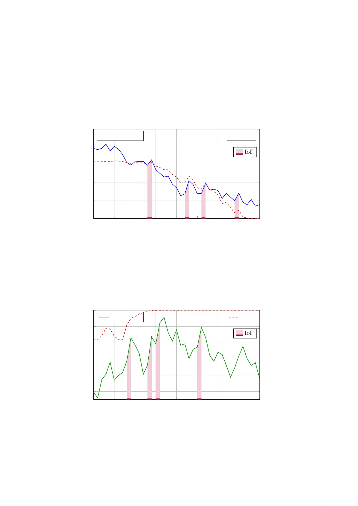
Real-time Win Probabilit y and Laten t Pla y er Abilit y via ST A TS X in T eam Sp orts Y asutak a Shimizu ∗ , A tsushi Y amanob e Departmen t of Applied Mathematics, W aseda Universit y F ebruary 24, 2026 Abstract This study prop oses a statistically grounded framework for real-time win probabilit y ev al- uation and play er assessmen t in score-based team sp orts, based on minute-b y-min ute cumula- tiv e box-score data. W e in tro duce a contin uous dominance indicator (T-score) that maps final scores to real v alues consistent with win/lose outcomes, and formulate it as a time-evolving sto c hastic represen tation (T-pro cess) driv en b y standardized cum ulative statistics. This struc- ture captures temp oral game dynamics and enables sequential, analytically tractable up dates of in-game win probability . Through this sto c hastic formulation, comp etitiv e adv antage is decomp osed into interpretable statistical comp onents. F urthermore, w e define a latent con- tribution index, ST A TS X, whic h quantifies a pla yer’s inv olvemen t in fav orable dominance in terv als identified by the T-process. This allows us to separate a team’s baseline strength from game-sp ecific p erformance fluctuations and provides a coherent, structural ev aluation framew ork for b oth teams and play ers. While w e do not implemen t AI metho ds in this pa- p er, our framework is p ositioned as a foundational step tow ard hybrid integration with AI. By providing a structured time-series represen tation of dominance with an explicit probabilis- tic interpretation, the framework enables flexible learning mec hanisms and incorp oration of high-dimensional data, while preserving statistical coherence and in terpretability . This work pro vides a basis for adv ancing AI-driven sp orts analytics. Keywor ds: sp orts statistics, statistical ST A TS, latent contribution, dynamic win probability , sto c hastic pro cess mo del, MSC2010: 62P25 ; 60G99, 68T05. 1 In tro duction In recent years, with the rapid developmen t of artificial in telligence technologies, the use of data in sp orts has entered a p eriod of ma jor transformation. T actical analysis based on tracking data and sensor information, outcome prediction using deep learning, and strategy exploration via reinforcemen t learning hav e adv anced significan tly , and sophisticated analytical infrastructures are b eing established in professional environmen ts. Within this broader mov emen t, interdisciplinary informatics fo cused on sp orts, namely “sp orts informatics,” is emerging as a nascent academic field. Ho wev er, in many amateur settings and developmen tal environmen ts, only limited game statis- tics (hereafter referred to as ST A TS) are recorded, and p ost-game play er ev aluations are often conducted based on coac hes’ sub jective judgmen ts. Even in professional con texts, critical decisions ∗ shimizu@waseda.jp 1 suc h as in-game substitution choices, timeout calls, ev aluation of young pla yers, and assessments of future v alue directly linked to contract negotiations remain challenging problems. In such situa- tions, a statistically grounded theoretical framework is required in order to make rational decisions from limited information. Existing performance metrics widely used in practice p ossess structural limitations. T aking bas- k etball as an example, commonly used indices such as EFF and PER are static measures formed as linear combinations of aggregated quantities such as p oints and reb ounds, and they do not explic- itly accoun t for temp oral structure or context dep endence. Because their structure is dominated by scoring contributions, they are unable to adequately ev aluate contributions that form or sustain the real-time “flow” of a game, particularly in crucial moments, as well as indirect effects that are not explicitly recorded in the statistics. Metrics such as plus-minus measure p oin t differentials while a play er is on the court, but they cannot disen tangle the influence of simultaneously participating teammates and lack a theoretical framework that decomp oses structural ability and within-game fluctuations. These issues stem from the fact that existing metrics do not explicitly mo del their relationship with game outcomes as a statistical structure. In particular, it is difficult to handle the effect of “flo w,” which inherently p ossesses temp oral dep endence, using only conv entional ST A TS. T o address these challenges, the present study reconstructs existing ST A TS within a statistical framew ork and introduces an ev aluation system that can b e interpreted based on its relationship with game outcomes. Sp ecifically , discrete outcomes such as win/loss results or score differentials are mapp ed to a contin uous measure of adv antage, which is then treated as the resp onse v ariable in estimating its relationship with ST A TS. F urthermore, by extending the ev aluation to a time- ev olution mo del, we dynamically capture changes in adv antage during a game, thereby indirectly extracting contributions that are difficult to assess using static aggregate metrics. The starting p oin t of this study is the light weigh t mo del prop osed in [Y amanob e 24]. That mo del emphasized a simple structure that can b e computed in real time even by amateur teams at the elementary and junior high school levels, and it presented a framework for outcome predic- tion and play er ev aluation based solely on limited ST A TS. In the present pap er, while preserving its fundamental philosoph y , we clarify the theoretical structure and incorp orate consistency b e- t ween the dynamic adv antage pro cess and the win probability function. In doing so, w e develop a generalizable and extensible ev aluation system that aims to reconcile “a light weigh t statistical infrastructure implementable in practice” with “compatibility for integration with artificial intel- ligence technologies.” Although this pap er do es not attempt a full AI implementation and adopts relativ ely simple statistical mo dels, v arious AI-based extensions can naturally b e envisioned, including nonlinear ev aluation functions, integration with deep time-series mo dels, strategy optimization through re- inforcemen t learning, and connections to causal inference. The prop osed framew ork do es not comp ete with AI; rather, it provides an interpretable foundational mo del that supp orts further sophistication through AI. F or the empirical analysis, we use official game data sp ecially provided for the Sp orts Data Science Comp etition organized b y the Sp orts Statistics Section of the Japanese Statistical So ciet y . These data are rare and sub ject to contractual distribution restrictions, and they consist of high- qualit y records based on actual measurements. Utilizing this v aluable dataset, we demonstrate cases in whic h pla yers who were not adequately ev aluated b y existing metrics are re-ev aluated under the prop osed framework. This study challenges the quantification of in-game “flow” and con text-dep enden t contributions, whic h ha ve b een difficult to capture using publicly a v ailable statistical indices, and seeks to connect practical decision-making in the field with statistical theory . As a foundational contribution to the emerging field of sp orts informatics, w e aim to present an ev aluation system that simultaneously 2 satisfies implementabilit y , statistical v alidity , and compatibility with AI in tegration. 2 T eam P erformance Index: T-score 2.1 Ev aluation of Outcome Sup eriorit y: T-score F unction Consider a team sp ort in which the outcome is determined by the score. Let a ≥ 0 denote the p oin ts scored by our team and b ≥ 0 denote the p oin ts conceded. In this study , in order to map the game result (discrete scores) to a contin uous measure of sup eriorit y , we introduce a function T : [0 , ∞ ) 2 → R and ev aluate the extent to whic h our team held an adv antage in the game through the v alue T ( a, b ). Definition 2.1. Given a function T : [0 , ∞ ) 2 → R , if there exists a constant c ∈ R suc h that for an y x ≥ 0 T ( x, x ) = c and, for any a, b ≥ 0, a > b ⇐ ⇒ T ( a, b ) > c a = b ⇐ ⇒ T ( a, b ) = c a < b ⇐ ⇒ T ( a, b ) < c, then the function T is called a T-score function , and the v alue T ( a, b ) is called the T-score . Remark 2.1. The constan t c serv es as the “dra w b enc hmark v alue.” In principle, the function T is c hosen so that the larger T ( a, b ) is ab ov e c , the more decisive the victory , and the further T ( a, b ) is b elo w c , the more decisiv e the defeat. Therefore, if the T-score can b e predicted, one can ev aluate not only the binary outcome (win/loss) but also the degree of winning or losing in a con tinuous manner. 2.2 Concrete Examples of T-score F unctions Belo w, w e presen t representativ e examples of T-score functions and explain their statistical meaning and appropriate applications. All of them satisfy T ( x, x ) = c and are consistent with the direction of sup eriorit y in terms of ordering. Example 2.1 (Simple score difference and ratio type) . T ( a, b ) = a − b, c = 0 . This is the simplest form, where a draw is represented by T = 0. It is a natural choice for sp orts with relatively low scores and limited v ariation in total p oin ts across games, suc h as so ccer. On the other hand, in high-scoring sp orts suc h as basketball, the score difference tends to dep end on the ov erall scale of the game. In such cases, a score ratio type ma y b e considered: T ( a, b ) = a b . In this case, the draw b enc hmark is c = 1. How ever, this simple ratio form has certain drawbac ks, and a mo dified version is presented in the following example. 3 − 1 − 0 . 5 0 0 . 5 1 − 1 − 0 . 5 0 0 . 5 1 log( a/b ) T ( a, b ) − 1 Figure 1: Deviation of the corrected T-score from the baseline v alue 1 Example 2.2 (Symmetric correction of score ratio) . The simple score ratio ab ov e has the dra wback that the distance from the draw b enchmark v alue 1 is asymmetric b et ween the winning and losing sides. F or example, when a = 120 , b = 100, we hav e a/b = 1 . 2, and the distance from the b enc hmark is 0 . 2. On the other hand, when a = 100 , b = 120, w e ha ve a/b = 0 . 833 . . . , and the distance from the b enchmark is 0 . 166 . . . . Th us, even with the same score difference of 20, the distances from the b enchmark do not coincide b etw een winning and losing cases. In this wa y , the simple score ratio do es not provide a symmetric ev aluation centered at the b enc hmark v alue 1, and therefore lacks geometric consistency when the strength of victory or defeat is interpreted as a “distance.” In particular, when a > b , w e hav e T ( a, b ) − 1 = ( a − b ) /b , where the denominator is alwa ys the smaller score b , which tends to ov erstate the winning side relativ e to the losing side. T o address this issue, while retaining the draw b enc hmark c = 1, w e consider the following mo dification so that th e deviation from the benchmark b ecomes symmetric with respect to winning and losing: T ( a, b ) =  2 − b a  1 { a ≥ b } + a b 1 { b>a } , c = 1 . (2.1) Under this definition, | T ( a, b ) − 1 | = | a − b | max( a, b ) holds, and the distance from the draw b enchmark coincides with the score difference normalized b y the larger of the tw o scores. 1 plots log( a/b ) on the horizontal axis and T ( a, b ) − 1 on the vertical axis. The condition log( a/b ) = 0 corresp onds to a = b and thus represents the dra w b enc hmark v alue c = 1. The fact that this graph is symmetric with resp ect to the origin means that T ( a, b ) − 1 = − ( T ( b, a ) − 1) , that is, the sup eriorit y when the ratio a/b > 1 and the inferiority for its recipro cal b/a hav e equal distances from the benchmark, differing only in sign, whic h is the so-called antisymmetry 4 prop ert y . The simple score ratio a/b do es not p ossess this antisymmetry , resulting in a distortion of ev aluation b etw een the winning and losing sides. In this pap er, we analyze a basketball example in Section 7, where we adopt the T-score given in (2.1). Example 2.3 (Log-ratio type) . T ( a, b ) = log a + κ b + κ , κ > 0 , c = 0 . This form applies a logarithmic transformation to the score ratio and satisfies T ( a, b ) = − T ( b, a ) (an tisymmetry), thereby resolving the asymmetry issue of the simple score ratio. It has strong theoretical consistency for low-scoring sp orts or in situations where scores are assumed to arise according to Poisson pro cesses. The parameter κ is a stabilization constan t for zero scores, but its choice requires care. F or example, when κ = 0, the relation T ( λa, λb ) = T ( a, b ) holds for any λ > 0, whic h implies so-called “scale inv ariance.” How ever, when κ > 0, in general T ( λa, λb )  = T ( a, b ) , and in particular, κ affects the v alue in low-scoring regimes. Th us, κ may b e interpreted as a regularization parameter that balances stabilization at zero scores and scale in v ariance. Example 2.4 (Relative difference t yp e) . T ( a, b ) = a − b a + b + κ , κ > 0 , c = 0 . This form constrains the score difference to the in terv al ( − 1 , 1) and mitigates the influence of game scale. In high-scoring sp orts, it enables comparability across games with different scoring levels, and is therefore suitable, for example, for rugby or American fo otball. By normalizing the score difference by the total score, the range b ecomes − 1 < T ( a, b ) < 1, preven ting extreme v alues. Moreo ver, since T ( b, a ) = − T ( a, b ) holds, the function satisfies an tisymmetry , although it do es not p ossess scale in v ariance. In particular, κ > 0 becomes dominan t in low-scoring regions. In addition, large-margin games are difficult to distinguish. F or example, comparing tw o lopsided games, 40–0 , 80–0 , w e obtain T (40 , 0) = 40 40 = 1 , T (80 , 0) = 80 80 = 1 , so the tw o cases are indistinguishable. Therefore, the prop erty describ ed in Remark 2.1 is not satisfied. The following example provides a mo dification to address this issue. Example 2.5 (Normalized type) . T ( a, b ) = a − b √ a + b + κ , This T-score can b e interpreted as an asymptotically standardized statistic of the score difference when the scores are approximated by Poisson distributions (with δ > 0 introduced to stabilize the denominator): assume that the scores are indep enden tly distributed as a n ∼ P o ( λ 1 ,n ) , b n ∼ P o ( λ 2 ,n ) , 5 and that λ 1 ,n + λ 2 ,n → ∞ . Then E [ a n − b n ] = λ 1 ,n − λ 2 ,n , V ar( a n − b n ) = λ 1 ,n + λ 2 ,n . By the central limit theorem, a n − b n − ( λ 1 ,n − λ 2 ,n ) p λ 1 ,n + λ 2 ,n d − → N (0 , 1) . In particular, for evenly matched teams under the assumption λ 1 ,n = λ 2 ,n , a n − b n p λ 1 ,n + λ 2 ,n d − → N (0 , 1) . F urthermore, a n + b n λ 1 ,n + λ 2 ,n p − → 1 , and hence, by Slutsky’s theorem, a n − b n √ a n + b n d − → N (0 , 1) , n → ∞ , whic h explains the meaning of the normalization. Using the same numerical example as in Example 2.4, 40 √ 40 = √ 40 ≈ 6 . 32 , 80 √ 80 = √ 80 ≈ 8 . 94 , so the T-score increases as the scale of the game increases, making it suitable for high-scoring sp orts in which the num b er of scoring even ts is large. 3 A General Nonlinear Mo del for the T-score and Statistical Strength Ev aluation 3.1 T eam-wise Mo deling of the T-score In what follows, Let T k denote the (end-of-game) T-score for Game k , and write the vector of “standardized” cumulativ e ST A TS of d types as S k := ( S k 1 , . . . , S k d ) ⊤ . Remark 3.1. Here, “standardization” refers to the “diffusion standardization” defined later in 4.1 and Definition 4.1. Ho wev er, diffusion standardization based on the final cumulativ e ST A TS after the game coincides with the usual “normalization (standardization)” given by S k i − E [ S k i ] √ V ar( S k i ) . Therefore, within this section, “standardization” ma y be understo o d as the ordinary normalization that makes the mean 0 and the v ariance 1. Note also that the “standardization” of ST A TS b efore the game starts is given by Definition 4.1 as S k = (0 , 0 , . . . , 0) ⊤ . Assumption 1. The T-score T k of Game k is determined by d types of ST A TS and admits a general regression structure from S k to T k : there exist parameters α 0 ∈ R , α = ( α 1 , . . . , α p ) ⊤ ∈ R p and a nonlinear function F α : R d → R satisfying F α (0 , 0 , . . . , 0) = 0 (3.1) 6 suc h that T k = α 0 + F α ( S k 1 , . . . , S k d ) + ε k . (3.2) Here, ε k is an I ID noise sequence with mean 0 and v ariance σ 2 . Since all ST A TS are 0 b efore the game starts, b y Remark 3.1 and condition (3.1), w e hav e E [ T k ] = α 0 , and α 0 can b e viewed as the basic (av erage) T-score that the team p ossesses from the outset. A team with a larger v alue of α 0 is in terpreted as ha ving a greater initial adv antage already at the start of the game, and thus α 0 can b e interpreted as represen ting the team’s fundamental strength. Definition 3.1. The av erage T-score that a team p ossesses before the game starts, T F S := α 0 , (3.3) is called the T eam F undamental Score (TFS) . On the other hand, the term F α ( S k 1 , . . . , S k d ) is a score added as ST A TS accumulate, and ma y b e regarded as a game-sp ecific statistical score. Definition 3.2. In Game k , the score added according to the team’s ov erall ST A TS ( S k 1 , . . . , S k d ), T S S k := F α ( S k 1 , . . . , S k d ) , (3.4) is called the T eam Statistical Score (TSS) for Game k . 3.2 Pla y er-wise Mo deling of the T-score Under the general regression mo del for the team T-score, w e consider a T-score based on individual ST A TS. Assuming that the team T-score is given by the sum of play er contributions in each game, w e p ostulate the follo wing additive mo del. Assumption 2. Supp ose that the team in Game k has J play ers who app ear in the game. Then the team T-score is determined b y the sum of individual T-scores, and eac h play er’s T-score admits a general regression structure with resp ect to the pla yer’s ST A TS. That is, there exists a common function f α : R d → R for play ers j ∈ { 1 , 2 , . . . , J } such that T k = α 0 + J X j =1 f α ( S k,j 1 , . . . , S k,j d ) + ε k (3.5) holds. Here, α 0 and α = ( α 1 , . . . , α p ) ⊤ are the same parameters as in Assumption 1, and S k,j i denotes the i -th comp onent of the (standardized) ST A TS of pla yer j in Game k . Remark 3.2. The common choice of f α is adopted to ensure that the same ST A TS are ev aluated in the same wa y across play ers. Definition 3.3. In Game k , the score added to play er j according to the pla y er’s ST A TS ( S k,j 1 , . . . , S k,j d ), P S S k,j = f α ( S k,j 1 , . . . S k,j d ) , j = 1 , 2 , . . . , J, (3.6) is called the Play er Statistical Score (PSS) of play er j in Game k . In particular, T S S k = J X j =1 P S S k,j . 7 Definition 3.4. The contribution of play er j in Game k is defined by P C S k,j := α 0 J + α 0 P S S k,j − T S S k /J D k 1 { D k > 0 } , (3.7) where D k := J X j =1 | P S S k,j − T S S k /J | . W e call P C S k,j the Play er Con tribution Score (PCS) of play er j in Game k . Although the definition of P C S k,j ma y lo ok somewhat complicated, it is motiv ated as follows: • The first term α 0 /J represents a “baseline share,” namely an equal allo cation of TFS across pla yers. That is, eac h pla yer is regarded as having the same basic v alue prior to the start of the game. • The second term measures the deviation of the play er’s statistical contribution in that game from the team a verage, and uses it as a w eight to redistribute α 0 across the J play ers. Indeed, J X j =1 ( P S S k,j − T S S k /J ) = 0 , and if D k > 0 1 then J X j =1 P C S k,j = α 0 , J X j =1     P S S k,j − T S S k /J D k     = 1 . In this sense, P C S k,j is obtained by adding, to the “equal allocation of the team’s fundamen tal strength,” a quantit y in which the within-game statistical deviations are reallo cated as relative w eights. Therefore, PCS is not so m uch an estimator of long-run ability , but rather an index pro viding a within-team relative ev aluation in each game, and can b e interpreted as describing a p erformance allo cation structure under game-by-game scale adjustment. Since PCS weigh ts each PSS by its distance from the center (mean) of the PSS v alues, play er ev aluation should essentially b e based on PCS. 4 Dynamic Mo deling of the T-score The T-score defined ab ov e is a single index at the end of the game. In this study , we extend it to a sto c hastic pro cess that evolv es ov er time, called the “T-pro cess.” That is, we regard p erformance as fluctuating ov er the course of a game due to b oth deterministic and random comp onen ts. The deterministic comp onen t is sp ecified by the function representing the con tributions of each ST A TS, F α : R d → R . The random comp onen t is mo deled as a contin uous-time random fluctuation. 1 D k = 0 ⇔ P S S k, 1 = · · · = P S S k,J . 8 Sym b ol T arget level Meaning and role TFS T eam (pre-game) F undamental a verage strength possessed by the team be- fore the game starts. Represen ts long-run team funda- men tal strength. TSS T eam (p ost-game) Score added by the team’s ov erall statistical outcomes in the game. Represents game-sp ecific p erformance. PSS Individual (p ost-game) Pla yer’s individual statistical con tribution in the game. Constitutes comp onents of the team statistical score. PCS Individual (in-game ev aluation) Pla yer ev aluation v alue obtained by adding the within- game relative contribution to the equal allo cation of the team’s fundamental strength. Represen ts the game-by- game allo cation structure. T able 1: Conceptual organization of indices in the T-score framework 4.1 On the “Standardization” of Cum ulative ST A TS T o define the T-pro cess, w e would lik e to sp ecify a certain form of “standardized ST A TS,” not only to av oid having to consider differences in units across ST A TS, but also to mak e them consistently comparable throughout the time evolution. Belo w, let the ( i -th) cumulativ e ST A TS from the start of the game ( t = 0) to the end of the game ( t = 1) at time t ∈ [0 , 1] b e denoted by S i = ( S i ( t )) t ∈ [0 , 1] . W e then introduce a scaling rule that accounts for time evolution. Definition 4.1. Let e S i ( t ) denote the ( i -th) cumulativ e ST A TS at time t ∈ [0 , 1], and set m i := E [ e S i (1)] , v 2 i := V ar( e S i (1)) . Define S i ( t ) := e S i ( t ) − m i t v i . W e call this the diffusion standardization of the ST A TS pro cess S i = ( S i ( t )) t ∈ [0 , 1] . In particular, S i (0) = 0, and S i (1) = e S i (1) − m i v i (4.1) corresp onds to the usual normalization of the final ST A TS in the game. Remark 4.1. The “standardization” used in Section 3 concerned p ost-game ST A TS, and hence coincides with the standardization in the sense of (4.1). W e now explain the motiv ation for the term “diffusion standardization.” This s tandardization differs from the usual “standardization” that normalizes the v ariance to 1 at each time: e S i ( t ) − E [ e S i ( t )] q V ar( e S i ( t )) = e S i ( t ) − m i t v i √ t , 9 and it is inten tional that the denominator in diffusion standardization do es not include √ t . If e S i is a Poisson-t yp e pro cess with intensit y λ i 2 , then the diffusion-standardized pro cess { S i ( t ) } t ∈ [0 , 1] has a v ariance structure prop ortional to time, namely V ar( S i ( t )) ∝ t . Since this matc hes the v ariance structure of Brownian motion, S i ( t ) can b e appro ximated by a diffusion limit under high-frequency regimes ( λ i → ∞ ). Indeed, if e S i is a comp ound P oisson pro cess, one can pro ve that its diffusion standardization S i con verges weakly to a standard Bro wnian motion on a function space under a high-frequency limit (see the next example 4.1). Later, w e will exploit this fact to p erform dynamic mo deling of the T-score, whic h enables prediction of future T-scores and, as a byproduct, prediction of the win probability . Example 4.1 (A probabilistic mo del for cumulativ e ST A TS pro cesses) . In many team sp orts, the cumulativ e ST A TS pro cess e S i ( t ) can b e regarded as an in teger-v alued, nondecreasing, righ t- con tinuous pro cess. F or example, consider cumulativ e p oin ts in bask etball. The num b er of made shots is a point pro- cess N = ( N t ) t ∈ [0 , 1] . Let X k denote the points scored on the k -th scoring ev en t. Then { X k } k =1 , 2 ,... is an I ID sequence taking v alues 1 (free throw), 2 (regular field goal), or 3 (three-p oin t shot). The cum ulative score up to time t is then given b y e S ( t ) = N t X k =1 X k . Assume that N and X k are indep endent and that N is a P oisson pro cess with intensit y λ . Then S is a comp ound Poisson pro cess. Let E [ X 1 ] = m and V ar( X 1 ) = σ 2 , and apply diffusion standard- ization to e S . W e obtain S λ ( t ) := e S ( t ) − E [ e S ( t )] q V ar( e S (1)) = e S ( t ) − λmt p λ ( σ 2 + m 2 ) . No w consider the high-intensit y limit ( λ → ∞ ) 3 . Then the follo wing holds for the h -time increment of S λ : for any t, h > 0, by the (functional) cen tral limit theorem, S λ ( t + h ) − S λ ( t ) = e S ( t + h ) − λm ( t + h ) p λ ( σ 2 + m 2 ) − e S ( t ) − λmt p λ ( σ 2 + m 2 ) = e S ( t + h ) − e S ( t ) − λmh p λ ( σ 2 + m 2 ) h · √ h d − → N (0 , h ) , λ → ∞ . Th us, the h -increment of the diffusion-standardized pro cess S λ con verges in distribution to a normal distribution with mean 0 and v ariance h , whic h indicates that S λ con verges w eakly to a standard Brownian motion W = ( W t ) t ∈ [0 , 1] 4 (see, for example, [Billingsley 99]). More precisely , for any t ∈ [0 , 1], S λ d − → W in D ([0 , 1]) , λ → ∞ , where D ([0 , 1]) denotes the space of functions that are right-con tin uous with left limits. 2 F or man y ST A TS in team sp orts, suc h an assumption ma y b e reasonable. 3 This is an approximation in which the num b er of successful scoring even ts is regarded as “large.” 4 More rigorously , one needs to establish tightness of S λ in the space D ([0 , 1]), whic h we omit here. 10 In this w ay , “diffusion standardization” can b e regarded as a natural scaling motiv ated by diffusion limits, which explains why we do not scale by the instantaneous standard deviation. In the next subsection, we use this fact to mo del the flow of a game dynamically . 4.2 Dynamic Mo deling of the T-score: T-pro cess Definition 4.2. Fix constants α 0 ∈ R and σ > 0. Let a ( t ) and b ( t ) denote the p oints scored and conceded at time t ∈ [0 , 1], resp ectiv ely . Define the T-score v alue at time t by T ( t ) := T ( a ( t ) , b ( t )) . The sto c hastic pro cess T = ( T ( t )) t ∈ [0 , 1] is called the T-pro cess. Assumption 3. The T-pro cess T = ( T ( t )) t ∈ [0 , 1] satisfies the follo wing: for the function F α in Assumption 1, T ( t ) = α 0 + F α  S 1 ( t ) , . . . , S d ( t )  + σ ϵ ( t ) , t ∈ [0 , 1] , (4.2) where ϵ = ( ϵ ( t )) t ∈ [0 , 1] is a standard Brownian motion. Remark 4.2. In particular, b efore the game starts ( t = 0), w e hav e T (0) = α 0 , and after the game ends ( t = 1) the mo del coincides with (3.2), so the form ulation is consisten t. The T-pro cess is a dynamic mo del that sim ultaneously describ es structural changes in p erfor- mance driven by ST A TS and random fluctuations inherent in game dev elopment. 4.3 A Mo dification of the T-pro cess: mo dified T-pro cess The T-pro cess describ es the temp oral ev olution of a single team’s p erformance, but in actual games, ev aluation is alw ays determined in a relative relationship with the opp onen t. That is, even for the same performance, its contribution to winning can differ depending on the opponent’s fundamen tal strength. Let α 0 denote our team’s TFS and β 0 denote the opp onen t’s TFS. It is natural to represent the initial adv antage based on their difference, using the same T-score function as in the definition of TFS, as T ( α 0 , β 0 ) . This constant represents the relative sup eriorit y at the start of the game in the sense of the given T -score function. Therefore, when we interpret the flow of a game that incorp orates the opp onen t through changes in the T-score, it is natural to replace the initial v alue α 0 b y T ( α 0 , β 0 ). Accordingly , we prop ose the following mo dified T-pro cess. Definition 4.3. Let α 0 b e our team’s TFS and β 0 the opp onen t’s TFS. F or t ∈ [0 , 1], define m T ( t ) = T ( α 0 , β 0 ) + F α  S 1 ( t ) , . . . , S d ( t )  + σ ϵ ( t ) . (4.3) The sto chastic pro cess m T = ( m T ( t )) t ∈ [0 , 1] is called the mo dified T-pro cess . The v alue m T ( t ) is called the mo dified T-score at time t . Since the m T -score pro vides a real-time (time- t -wise) quantification of p erformance, its increase or decrease is regarded as representing the team’s flow. When the m T -score falls b elow the draw b enc hmark v alue c (here c = 1), it is closer to “losing,” and when it exceeds c , it suggests moving closer to “winning.” Moreo ver, as discussed later, by predicting the future m T -score based on information up to time t as a sto chastic pro cess, we can also compute the “win probability” at time t . 11 4.4 F uture T-scores: predicted T-pro cess W e can use the m T -pro cess to grasp the flo w of a game and plan strategies. F or this purp ose, we consider as imp ortan t indicators the prediction of the m T -score at a future time u ( > t ) ev aluated at time t , and the win probability at time t . Definition 4.4. Let a := a ( t ) and b := b ( t ) denote the p oin ts scored and conceded at time t ∈ [0 , 1]. Define the filtration (history) F = ( F t ) t ∈ [0 , 1] b y F t := σ  S ( s ) , a ( s ) , b ( s ) : s ≤ t  . A t a given time t , define the predicted T-score at a future time u ∈ ( t, 1] by p T ( u | t ) := T ∗ ( t, a, b ) + { m T ( u ) − m T ( t ) } , (4.4) where T ∗ ( t, a, b ) := (1 − t ) T ( α 0 , β 0 ) + t T ( a, b ) . (4.5) The pro cess p T ( · | t ) = ( p T ( u | t )) u ∈ [ t, 1] is called the predicted T-pro cess at time t . The v alue p T ( u | t ) for u > t is called the predicted T-score at time u (as ev aluated at time t ). Remark 4.3. The definition of T ∗ ( t, a, b ) in (4.5) allocates the w eights in time b et ween the realized score T ( a, b ) at time t and the initial score T ( α 0 , β 0 ). This is an ad ho c assumption intended to emphasize the initial score when information (ST A TS) is scarce in the early stage, and to emphasize the sup eriorit y implied by the realized score after sufficien t information has accumulated in the later stage. It also serves as a device to stabilize the p T -pro cess against accidental fluctuations early in the game. Thus, the p T -score should not b e interpreted as a prediction in a strict sense, but rather as an index that incorp orates something like the “pre-game reputation,” and is closer to our intuitiv e sense of the game. Remark 4.4. W e add a remark on the structure of the predicted T-pro cess. First, T ∗ ( t, a, b ) is constructed solely from information observed up to time t , and hence is F t -measurable. Therefore, the current state can b e interpreted as b eing fully summarized by T ∗ ( t, a, b ). On the other hand, future uncertaint y is contained only in m T ( u ) − m T ( t ). That is, the decomp osition p T ( u | t ) = T ∗ ( t, a, b ) | {z } current b enchmark + m T ( u ) − m T ( t ) | {z } future fluctuation pro vides a structure that clearly separates “current information” from “future randomness.” F or example, if m T is an independent-incremen t pro cess, then the increment m T ( u ) − m T ( t ) is in- dep enden t of F t , and the future T-score can b e describ ed via the distribution of the increment term. This assumption is not artificial. Indeed, as seen in Example 4.1, cumulativ e ST A TS can b e appro ximated by Brownian motion after diffusion standardization. Moreo ver, if we c ho ose F α as a linear mo del, F α ( s 1 , . . . , s d ) = d X i =1 α i s i , then m T can b e appro ximated as a Brownian-motion-t yp e indep enden t-increment pro cess. Th us, this formulation is not a purely probabilistic assumption, but is adopted as a practical mo del that arises naturally under high-frequency approximations. 12 5 Computation of Real-Time Win Probabilit y By the definition of the T-score function, at the terminal time u = 1, the ev ent that the T- score exceeds the draw b enc hmark v alue c is equiv alent to winning the game. Therefore, the win probabilit y at time t is giv en by a conditional probability , under the information F t a v ailable up to time t , that the predicted T-score at the future time u = 1 exceeds c . Definition 5.1. W e define the (conditional) Probability of Win at time t by P W t := P  p T (1 | t ) > c   F t  . (5.1) Remark 5.1. Note that the quan tity P W t ab o ve is slightly differen t from the actual win probabil- it y . Indeed, the predicted T-pro cess p T ( u | t ) is constructed based on an ad ho c quan tity suc h as T ∗ , and do es not provide a strict prediction of the future T-score. Hence, the ab o ve is a “definition,” not a “theorem.” The quan tity P W t should b e understo od as what we approximately regard as the “win probability” (see also Remark 4.3). By computing this probabilit y sequentially at each time t as ST A TS accum ulate, we can vi- sualize in real time ho w the win probabilit y changes with the flow of the game. That is, P W t is not merely a p ost ho c ev aluation, but a “dynamic ev aluation index” that is con tinuously up- dated as the game progresses. It plays a role analogous to the “AI ev aluation v alue” display ed in shogi broadcasts. Not only coac hes but also sp ectators without sp ecialized tactical knowledge can intuitiv ely grasp whic h side is currently adv antaged, and how muc h eac h play shifts the win probabilit y . More imp ortan tly , P W t is defined based on a probabilistically coherent mo del. Therefore, it is not a heuristic metric, but a theoretically grounded real-time estimate of win probability ro oted in the probabilistic structure of cum ulative ST A TS. In particular, under certain conditions, we can obtain an explicit expression for P W t , as stated in the following theorem. Theorem 5.1. Let a ( t ) and b ( t ) denote the p oin ts scored and conceded at time t ∈ [0 , 1], resp ec- tiv ely . Assume the following: (a) The diffusion-standardized cumulativ e ST A TS pro cess ( S 1 ( t ) , . . . , S d ( t )) t ∈ [0 , 1] follo ws a d -dimensional standard Bro wnian motion. (b) The function F α is linear: F α ( s 1 , . . . , s d ) = α 1 s 1 + . . . α d s d , that is, the T-pro cess is giv en b y T ( t ) = α 0 + d X i =1 α i S i ( t ) + σ ϵ ( t ) , t ∈ [0 , 1] . Here, ϵ = ( ϵ ( t )) t ≥ 0 is a standard Brownian motion and is indep enden t of each S j . Then the win probability is expressed as P W t = 1 − Φ c − T ∗ ( t, a ( t ) , b ( t )) p (1 − t )( τ 2 + σ 2 ) ! (5.2) where c is the draw b enc hmark v alue, τ 2 = P d i =1 α 2 i , and Φ denotes the cumulativ e distribution function of the standard normal distribution. 13 Pr o of. By Assumption (b), note that m T ( u ) − m T ( t ) = d X i =1 α i ( S i ( u ) − S i ( t )) . By Assumption (a), S i ( u ) − S i ( t ) ∼ N (0 , u − t ) , i = 1 , . . . , d, and the increments S i ( u ) − S i ( t ) and S j ( u ) − S j ( t ) are indep enden t when i  = j . Therefore, m T ( u ) − m T ( t ) ∼ N  0 , ( u − t )( τ 2 + σ 2 )  , where τ 2 := P d i =1 α 2 i . Hence, p T (1 | t ) | F t ∼ N  T ∗ ( t, a ( t ) , b ( t )) , (1 − t )( τ 2 + σ 2 )  , and thus P W t = P ( p T (1 | t ) > c | F t ) = 1 − Φ c − T ∗ ( t, a ( t ) , b ( t )) p (1 − t )( τ 2 + σ 2 ) ! . This prov es the claim. Remark 5.2. F rom the win probabilit y formula (5.2), we hav e ∂ P W t ∂ S i = ϕ c − T ∗ ( t, a ( t ) , b ( t )) p (1 − t )( τ 2 + σ 2 ) ! α i p (1 − t )( τ 2 + σ 2 ) . (5.3) Here, ϕ ( x ) = Φ ′ ( x ) is the standard normal density . Therefore, α i > 0 not only con tributes to increasing the m T -pro cess, but also leads to an increase in P W t . 6 Ev aluation of Pla y ers’ Latent Ability: ST A TS X In this section, we formalize play ers’ laten t ST A TS “X,” whic h do not appear in conv entional ST A TS, as a transformed quantit y of a play er activit y index called the “X-index.” Using this, we prop ose a new ov erall play er ev aluation index, called the Play er T otal Score (PTS). First, we define the following X-index as a play er “activit y index.” Definition 6.1. Given ∆ = 1 /R ( R ∈ N ), set t r = r ∆ ( r = 0 , 1 , . . . , R ). W rite the m T -score at time t r in Game k as m T k ( t r ), and define R k δ :=  r = 0 , 1 , . . . , R − 1     ∆ ( r ) m T k ∆ > δ  , where ∆ ( r ) m T k := m T k ( t r +1 ) − m T k ( t r ). Then the follo wing subinterv al is called the δ -Interv al on Fire : I oF k δ := [ r ∈R k δ [ t r , t r +1 ) ⊂ [0 , 1] . Let I k,j ⊂ [0 , 1] denote the time interv al during which pla yer j was on the court in Game k . Define X k,j δ := Z I k,j 1 I oF k δ ( t ) dt, and call it the X-index of play er j in Game k . 14 This X-index indicates the fraction of time during whic h the play er was on the court when the game was in a “go o d flo w,” and 0 ≤ X k,j δ ≤ | I oF k δ | ≤ 1 holds. The quantit y X k,j δ measures ho w muc h of the game the play er participated in while b eing in an “On Fire” state. During I oF k δ , it is reasonable to regard all play ers on the court as sync hronizing and pro ducing go o d p erformance. Therefore, even if no ev ent is directly counted as ST A TS during that interv al, the idea is to view it as a p eriod in which every one was implicitly playing well, and to aw ard uniform p oin ts to the play ers who were on the court in that interv al. Definition 6.2. (i) F or a given function h : [0 , 1] → R , the transformed v alue of the X-index X k,j δ , namely h ( X k,j δ ), is called ST A TS X of play er j in Game k (based on h ). (ii) The ov erall con tribution aggregated ov er n games is defined by P T S j := 1 n n X k =1 [ P C S k,j + h ( X k,j )] , (6.1) and is called the Play er T otal Score (PTS) . Remark 6.1. The function h determines the exten t to whic h the ev aluation of “goo d flow” is incor- p orated, and can b e chosen freely dep ending on the team’s ev aluation criteria. F rom a theoretical viewp oin t, it is desirable that h satisfies the follo wing prop erties. (1) Normalization condition : h (0) = 0 . No additional ev aluation is assigned to a play er who is not inv olved in IoF at all. (2) Monotonicit y : x 1 < x 2 ⇒ h ( x 1 ) ≤ h ( x 2 ) . This guarantees that longer inv olv ement in go o d flow leads to higher ev aluation. (3) Boundedness : There exists a constant C > 0 such that | h ( x ) | ≤ C ( x ∈ [0 , 1]) . This keeps h ( X k,j δ ) on a scale comparable to the existing P S S k,j and P C S k,j , and ensures stabilit y of the ov erall ev aluation. (4) Con tinuit y : The function h is contin uous on [0 , 1]. This prev ents the ev aluation v alue from jumping discontin uously in resp onse to small changes in IoF. (5) Con vexit y or concavit y (strategy-dep endent) : If h is c hosen to b e conv ex, the design emphasizes long inv olvemen t in IoF, whereas if h is concav e, the design relativ ely rewards pla yers who are inv olv ed in IoF even for a short time. Remark 6.2. A linear choice, h ( x ) = κx ( κ > 0 , x ∈ [0 , 1]) , is the simplest y et pow erful option that adds flo w contribution with a constan t w eight. F or selecting the constant κ , one natural option is to set κ = δ 15 based on the threshold δ used in defining the X-index. Indeed, by the definition of δ -IoF, if r ∈ R k δ , then ∆ ( r ) m T k > δ ∆ holds. If a set A ⊂ I oF k δ is a finite union of in terv als of the form [ t r , t r +1 ), then X r : [ t r ,t r +1 ) ⊂ A ∆ ( r ) m T k > δ | A | . In particular, letting A = I k,j ∩ I oF k δ , we obtain X r : [ t r ,t r +1 ) ⊂ I k,j ∩ I oF k δ ∆ ( r ) m T k > δ X k,j δ . Th us, δ X k,j δ can b e interpreted as a quantit y giving a low er b ound for the incremen t of the m T - pro cess o ver the time interv als during which the play er is inv olved in IoF. In the basketball data analysis presen ted later, we adopt this linear form. 7 Real Data Analysis: Basketball The data used in this study consist of the 2022–2023 season of the Japanese professional bask etball B1 League (from the official B.League website [BLeague]), as well as the play-b y-play data and b o x-score data for eac h team in the 2022–2023 season provided by Data Stadium Inc. In what follows, we analyze the regular season ( n = 60 games) using the following eight repre- sen tative ST A TS. S k 1 : Poin ts (PTs) S k 5 : Offence Reb ound (OR) S k 2 : Field Goal Made (FGM) S k 6 : Assists (AS) S k 3 : Three Poin ts FGM (3FGM) S k 7 : T urn Over (TO) S k 4 : Defence Reb ound (DR) S k 8 : F oul Drawn (FD) T able 2: Definition of ST A TS { S k i } i =1 ,..., 8 in game k F or mo deling the T -pro cess, w e adopt the following sp ecifications: • As the T-score function, we use (2.1): T ( a, b ) =  2 − b a  1 { a ≥ b } + a b 1 { b>a } . • T o mo del the T-score, we employ a linear mo del for F α : R 8 → R with ε k ∼ (0 , σ 2 ) (I ID): T k = α 0 + α 1 S k 1 + · · · + α 8 S k 8 + ε k . Accordingly , using the play er-level ST A TS ( S k,j ), we hav e T k = α 0 + J X j =1 n α 1 S k,j 1 + · · · + α 8 S k,j 8 o + ε k . 16 • Let α 0:8 := ( α 0 , α 1 , . . . , α 8 ) b e unknown parameters. W e estimate them b y the least squares metho d: b α 0:8 = arg min α 0:8 ∈ Π n X k =1   Y k −  α 0 + α 1 S k 1 + · · · + α 8 S k 8    2 , (7.1) where Π is a sufficiently large b ounded closed subset of R 9 . • The function defining ST A TS X is given by h ( x ) = δ x, δ > 0 , and the v alue of δ is determined for each game (as describ ed later). The analysis pro ceeds as follo ws: 1. Using the ST A TS from all regular-season games in 2022–2023 ( n = 60), we compare the estimated v alues of T F S = α 0 across teams and examine whether they are consistent with the interpretation of “team fundamental strength.” (7.1) 2. F or the top-rank ed team in winning p ercen tage, “Chiba Jets,” we estimate the parameters α 0:8 and discuss the team’s characteristics based on the estimated co efficien ts. (7.2) 3. F o cusing on several games of the “Chiba Jets,” w e plot the m T -pro cess and the corresp onding win probability P W t deriv ed from the estimated mo del, and discuss their relationship. (7.3) 4. F or the ab ov e games, we compute pla yer ev aluations b oth without ST A TS X (PCS) and with ST A TS X (PTS), and compare them with existing play er ev aluation metrics such as ETF and PER. (7.4) 7.1 Comparison of T eam F undamen tal Strength Using TFS By definition, TFS ( α 0 ) is the parameter that determines the initial level of the T-pro cess at the start of the game, and represents a “prior fundamen tal adv an tage” that exists indep enden tly of the dynamic comp onen t (the F α term). F rom the table of TFS v alues (3) and the scatter plot (2), the correlation co efficien t b et ween winning p ercentage and α 0 is ρ = 0 . 989, which is nearly 1. In particular, for the top teams such as Chiba ( α 0 = 1 . 141, winning p ercen tage 0 . 883), Ryukyu ( α 0 = 1 . 088, winning p ercen tage 0 . 800), and Nagoy a ( α 0 = 1 . 086, winning p ercen tage 0 . 716), w e observ e clearly that α 0 > 1. On the other hand, for lo wer-rank ed teams such as Osak a ( α 0 = 0 . 977), Kyoto ( α 0 = 0 . 952), and Niigata ( α 0 = 0 . 875), we hav e α 0 < 1. These findings suggest that α 0 is not merely a fitting coefficient, but rather quan tifies the relativ e fundamen tal strength within the league, supp orting the in terpretation that α 0 represen ts team fundamental strength. When α 0 is larger than the opp onen t’s, the mo dified T-score m T (0) starts ab o ve 1 by construc- tion. This represents a pre-game adv antage against the opp onen t, and th us P W t starts ab ov e 0 . 5 at game start. F or example, for the top-win-rate team Chiba Jets, T able 4 shows that m T (0) > 1 against every opp onen t, implying P W t > 0 . 5 b efore the game b egins. 7.2 Estimation of α 0:8 for Chiba Jets. In this subsection, w e fo cus on Chiba Jets, the team with the highest win rate, and discuss parameter estimation and the influence of each ST A TS. T able 5 rep orts the estimation results. Note that the sign and statistical significance of each α i ( i = 0 , 1 , . . . , 8) indicate the direction and strength of the effect of each ST A TS on the m T -pro cess. 17 0 . 85 0 . 9 0 . 95 1 1 . 05 1 . 1 1 . 15 1 . 2 0 0 . 2 0 . 4 0 . 6 0 . 8 1 Chiba Ryukyu Nago ya Ka wasaki Osak a Ky oto Niigata T F S ( α 0 ) Win rate Figure 2: Scatter plot of T F S and win rate ( ρ = 0 . 989) T eam TFS( α 0 ) W–L Win rate Chiba 1.140517 53–7 0.883 Ryukyu 1.088059 48–12 0.800 Nago ya 1.086108 43–17 0.716 Ka wasaki 1.05268 40–20 0.666 Osak a 0.977479 27–33 0.450 Ky oto 0.952111 22–38 0.366 Niigata 0.874814 13–47 0.216 T able 3: Comparison of TFS ( α 0 ) and win rate Opp onen t β 0 (opp onen t TFS) α 0 (Chiba TFS) m T (0) Ryukyu 1.088059 1.140517 1.045995 Nago ya 1.086108 1.140517 1.047706 Ka wasaki 1.052680 1.140517 1.077015 Osak a 0.977479 1.140517 1.142951 Ky oto 0.952111 1.140517 1.165194 Niigata 0.874814 1.140517 1.232967 T able 4: Mo dified T-score m T (0) at game start relative to Chiba Jets ( α 0 = 1 . 140517) 18 LSE Std. Error t -v alue p -v alue TFS ( α 0 ) 1.140157 0.013296 85.752 < 2e-16 PTs ( α 1 ) 0.062776 0.020391 3.079 0.003175 F GM ( α 2 ) -0.019203 0.017117 -1.122 0.266533 3F GM ( α 3 ) 0.009615 0.016535 0.582 0.563142 OR ( α 4 ) -0.006753 0.014714 -0.459 0.647960 DR ( α 5 ) 0.056412 0.013568 4.158 0.000107 AS ( α 6 ) 0.006372 0.015492 0.411 0.682348 TO ( α 7 ) -0.010293 0.013796 -0.746 0.458627 FD ( α 8 ) -0.013582 0.014983 -0.906 0.368430 T able 5: Estimation results from 60 Chiba Jets games TFS ( α 0 ) It is strongly significant at the 5% lev el. The interpretation is as discussed in the previous subsection. PTs ( α 1 ) It is significant at the 5% level. Since α 1 > 0, an increase in p oints increases mT . It is imp ortan t that this remains significant even after controlling for other ST A TS. DR ( α 5 ) It is highly significant. Since α 5 > 0, defensiv e reb ounds are a ma jor factor increasing the m T -score. Moreo ver, | α 5 | ≈ | α 1 | suggests that the contribution of defensive reb ounds is comparable in imp ortance to scoring. Non-significan t v ariables FGM, 3FGM, OR, AS, TO, and FD are not statistically significant with p > 0 . 05 . • If Cov( P T s, F GM ) > 0 is large, multicollinearit y may render the individual co efficient of F GM insignificant. • The estimate for OR is b α 4 = − 0 . 006753, negative but not significant. Offensiv e reb ounds often increase when sho oting p ercentage is low, so confounding such as Cov( OR , F GM ) < 0 ma y o ccur. • TO has b α 7 < 0, which is directionally consistent with domain knowledge, but not significant. Ov erall, the approximation T = α 0 + 0 . 0628 P T s + 0 . 0564 DR + (others are not statistically distinguishable from 0) app ears reasonable. Indeed, applying stepwise v ariable selection by AIC using the R function step yields a similar conclusion. Th us, the primary drivers of the Chiba Jets’ m T -pro cess app ear to b e p oints (PTs) and defensiv e reb ounds (DR) . In summary , Chiba Jets ac hieve a strong mT -pro cess through: 1. extremely high baseline strength (large α 0 ), 2. scoring ability , 19 3. defensive reb ounds. In particular, the finding | α 5 | ≈ | α 1 | quantitativ ely suggests that defensiv e control, not only offense, supp orts their top win rate. Remark 7.1. In T able 5, the estimated OR co efficien t is negative but not significant ( p = 0 . 648), so under this dataset and linear mo del, the indep enden t contribution of OR is not distinguishable from 0. Moreov er, regression co efficients represent conditional effects given other ST A TS. Since OR can increase with missed shots, including FGM and PTs in a multiv ariate regression ma y cause residual OR to proxy “low offensive efficiency”, resulting in a negative sign. Hence, the sign in terpretation of OR should b e treated cautiously , and discussions of key drivers should b e based on significant PTs and DR. Remark 7.2 (Negative co efficien ts for seemingly p ositive ST A TS and index design) . As noted ab o ve, estimated co efficien ts for ST A TS that are usually interpreted as positive contributions can b ecome negative. This o ccurs b ecause regression co efficien ts are conditional effects with other co v ariates held fixed, and correlations/multicollinearit y among cov ariates can cause signs to differ from marginal effects. Therefore, directly reflecting co efficient signs in to a pla yer ev aluation index (PCS) may yield deductions inconsistent with domain knowledge. Possible design impro vemen ts include: (1) Orthogonalization: Regress the ST A TS on other related indices and use only the residual comp onen t for PCS, remo ving confounding effects. (2) Sign-constrained design: Imp ose nonnegativity constraints on contributions to PCS, or dis- allo w negative contributions, preserving monotonicit y based on domain kno wledge. (3) Rate/efficiency transformations: Normalize count-t yp e ST A TS by opp ortunities or attempts to separate pace and exogenous comp onen ts, reducing sign rev ersals. W e do not pursue these in this pap er, but they constitute imp ortant op en problems. 7.3 Strategic implications from the path relation of m T -pro cess and P W t In this section, w e fo cus on the follo wing t wo games of the Chiba Jets in the 2022–2023 season, and examine the relationship b et ween the time paths of the m T -pro cess and the win probability P W t , discussing strategic implications for game management as well as their connection to play er ev aluation. The following tw o games are from the 2022–2023 pla yoffs. After estimating the mo del based on the 60 regular-season games, w e apply it to predict and analyze these play off games. 1. vs. Ryukyu Golden Kings (game on 2023/5/28, Chiba Jets lost 73–88): Figure 3. 2. vs. Alv ark T okyo (game on 2023/4/30, Chiba Jets w on 94–66): Figure 4. Basic structure P W t is monotonically increasing in T ∗ := T ∗ ( t, a ( t ) , b ( t )), and 0 < ∂ P W t ∂ T ∗ = ϕ  c − T ∗ s ( t )  s ( t ) ≤ 1 √ 2 π 1 s ( t ) (7.2) where s ( t ) := p (1 − t )( τ 2 + σ 2 ). Thus, • if m T increases then P W t increases, 20 • since s ( t ) b ecomes smaller in the late game, the same change in m T pro duces a larger change in P W t , whic h is the k ey structural feature. Also, IoF represents “time in terv als where m T rises signifi- can tly”, and strategically corresp onds to “interv als where the team has control”. P ath interpretation for the Ryukyu game (loss) In the losing game, we observe: • IoF interv als are intermitten t and short, • there exist sharp decline interv als after rises in m T , • in the late game, m T trends down ward. Since s ( t ) ↓ 0 near the end, the magnitude of ∆ P W t = ϕ ( · ) s ( t ) ∆ T ∗ is amplified, so a small late-game drop in m T can cause a steep fall in P W t . Strategically , the loss can b e in terpreted as due to: • failure to sustain IoF in the late game, • inability to suppress “rev ersal” interv als where m T ′ < 0. P ath interpretation for the T oky o game (win) In the winning game, we observe: • sustained IoF interv als from early stages, • m T evolv es in an approximately monotone increasing manner, • m T remains at a high level near the end. In this case, there are long interv als with T ∗ ≫ c , leading to P W t ≈ 1 early . Hence, pushing m T ab o ve the baseline c early contributes to stabilizing win probability . Connection to play er ev aluation The X-index measures how muc h a play er is inv olved in IoF. In a winning game with long sustained IoF, pla yers with large X-index contribute to forming the rising interv als of m T . In a losing game, IoF is short and intermitten t, and P j X δ k,j tends to b e smaller. Thus, • PCS measures the magnitude of statistical outcomes, • X-index measures contribution to sustaining control, and these are consistent with the time structure of the m T -pro cess. Strategic implications The ab o ve suggests that the key to maximizing win probabilit y is: 1. how to create IoF interv als early , 2. how to suppress late-game interv als with m T ′ < 0, 3. how to optimize lineups featuring play ers who stay inv olv ed in IoF for long durations. That is, “winning can b e viewed as optimizing the duration of IoF”. 21 Figure 3: T ra jectories of m T -pro cess and P W t (vs. Ryukyu Golden Kings) 0 5 10 15 20 25 30 35 40 0 . 85 0 . 9 0 . 95 1 1 . 05 1 . 1 Time (min) m T -pro cess m T -pro cess IoF 0 0 . 2 0 . 4 0 . 6 0 . 8 1 P W t P W t Figure 4: T ransition of the m T -pro cess and P W t (vs Alv ark T okyo) 0 5 10 15 20 25 30 35 40 1 . 06 1 . 08 1 . 1 1 . 12 1 . 14 1 . 16 Time (min) m T -pro cess m T -pro cess IoF 0 0 . 2 0 . 4 0 . 6 0 . 8 1 P W t P W t 22 7.4 Pla y er ev aluation with the in tro duction of ST A TS X Next, w e examine the play er ev aluations in these tw o games. T ables 6 and 7 rep ort PCS and ST A TS X for each game. F rom these tables, w e observe that pla yers with high PCS do not necessarily hav e high ST A TS X, and con versely , pla yers with mid-lev el PCS may exhibit relativ ely large ST A TS X. This discrepancy arises from the essential difference in the quan tities measured. PCS reallo cates the baseline strength α 0 according to relative in-game performance and ev aluates the ov erall statistical output of a game, whereas the X -index measures playing time during IoF δ , that is, p eriods in which the m T -pro cess increases significantly . First, in the game vs. Ryukyu (6), PCS ranks T ogashi (0.221), Lo we (0.204), Smith (0.134), and Mo oney (0.127) in descending order, with the top group clearly separated. In contrast, ST A TS X is largest for Edwards (0.059), follow ed by Low e (0.044), Mo oney (0.044), and Hara (0.042). Notably , although Edwards has a mid-level PCS of 0.081, his X is the largest, indicating strong in volv ement in upw ard momentum phases. In other words, while his aggregate statistical output is not outstanding, he contributes substan tially during p erio ds when the team’s flow improv es. Next, in the game vs. Alv ark T okyo (7), Smith has the highest PCS (0.255) and also the highest ST A TS X (0.076). In this game, statistical output and momentum contribution coincide, concen trating b oth “p erformance-driv en” and “flo w-driven” effects in the same pla yer. Meanwhile, Nishim ura has PCS 0.087 and X = 0 . 070, showing relatively strong inv olvemen t in IoF interv als. Th us, the alignment betw een aggregate p erformance and flow con tribution v aries across games, indicating structural differences dep ending on game context. PTS is defined on a p er-game basis as P T S j = P C S j + h ( X j ) , h ( x ) = δ x. Here, h ( X j ) provides the low er b ound δ X j for the incremen t of the m T -pro cess during IoF in terv als. Hence, PTS in tegrates relativ e performance an d momen tum contribution into a dynamic ev aluation measure. Indeed, from 8, in the game vs. Ryukyu, the highest PTS is T ogashi (0.221), follow ed b y Lo we (0.204), Smith (0.134), and Mo oney (0.127). In this game, the X -index adjustment do es not substantially alter the ranking, and the structure remains p erformance-driven. In contrast, in the game vs. Alv ark T okyo, Smith remains the highest at 0.257, confirming that aggregate p erformance and flow contribution op erate in the same direction. F urthermore, T able 9 reveals clear differences from conv entional metrics. Under EFF, T ogashi ranks first, while Low e ranks fifth. Under PER, Smith ranks first and Lo we fourth, so Low e is not necessarily top-ranked by existing indices. This reflects the fact that additive metrics heavily dep enden t on total scoring may underv alue certain con tributions. How ever, Low e’s ST A TS X is 0.044, a relatively high v alue, indicating substantial in volv ement in IoF interv als. Consequently , he ranks second in PCS and maintains second in PTS, suggesting that he combines both statistical output and flow contribution. Similarly , Edwards is positioned mid-tier in conv entional EFF and PER, y et has the highest ST A TS X (0.059). In this particular game, how ever, δ is relatively small, so PTS does not dramati- cally elev ate his ranking. Th us, even when flow contribution exists, its impact on o verall ev aluation dep ends on the chosen weigh t δ . These findings make it evident that total statistical output  = dynamic contribution to win probability . EFF and PER are static metrics that ev aluate total statistics or efficiency without accounting for time structure or situational dep endence. In con trast, PTS is constructed consisten tly with the 23 temp oral structure of the m T -pro cess and P W t , incorp orating the timing of contributions as an ev aluation axis. Of course, b eing on the court during IoF do es not necessarily imply that a sp ecific play er alone generated the momentum; another play er ma y ha ve driven the increase. How ever, when aggregated o ver many games across a season, such coincidences are unlikely to p ersist systematically , and ST A TS X can meaningfully capture dynamic contributions to win probability . These results hav e imp ortant implications for salary assessment and con tract ev aluation of professional play ers. Comp ensation is often determined by visible metrics suc h as scoring totals or PER. How ev er, as shown here, contribu tions to momen tum formation ma y not be sufficien tly reflected in such static indicators. That said, the choice of h ( x ) = δ x remains op en to discussion. The selection of δ is somewhat arbitrary (in this study , based on the fourth-largest rate of c hange), and different choices may o veremphasize dynamic contributions. This asp ect inevitably reflects team preferences. Neverthe- less, introducing dynamic indicators provides the p oten tial to quantify play er v alue that has b een previously underestimated, thereby offering a foundation for more sophisticated play er ev aluation, con tract strategy , and roster construction. Pla yer PCS ST A TS X Y uki T ogashi 0.209108 0.044 Asato Ogaw a 0.036235 0.017 Vic Law 0.194218 0.044 F umio Nishimura 0.04238 0.015 T akuma Sato 0.085812 0.000 Ga vin Edwards 0.085812 0.059 Sh uta Hara 0.03758 0.042 John Mo oney 0.126809 0.044 Christopher Smith 0.132884 0.030 T able 6: Play er ev aluation v alues and ST A TS X (vs Ryukyu Golden Kings), δ = 0 . 0148. Pla yer PCS ST A TS X Y uki T ogashi 0.144944 0.027 Asato Ogaw a 0.121435 0.050 Vic Law 0.176123 0.047 Katsumi T ak ahashi 0.049197 0.000 F umio Nishimura 0.087941 0.070 T akuma Sato 0.073266 0.052 Ga vin Edwards 0.063762 0.047 Gaku Arao 0.041005 0.000 Sh uta Hara 0.13093 0.045 John Mo oney 0.134514 0.050 Christopher Smith 0.235613 0.076 Jaba Y oneyama 0.051284 0.021 T able 7: Play er ev aluation v alues and ST A TS X (vs Alv ark T okyo), δ = 0 . 0242. 24 Pla yer PTS 1 PTS 2 Y uki T ogashi 0.139536 0.121908 Asato Ogaw a 0.112269 0.144683 Vic Law 0.139535 0.142261 F umio Nishimura 0.109871 0.165034 T akuma Sato 0.095047 0.146867 Ga vin Edwards 0.154366 0.141532 Sh uta Hara 0.137340 0.140079 John Mo oney -0.014636 0.145410 Christopher Smith 0.124705 0.171094 T able 8: PTS 1 : vs Ryukyu, PTS 2 : vs Alv ark T okyo Rank PCS PTS EFF PER 1 T ogashi Edwards T ogashi Smith 2 La w T ogashi Smith T ogashi 3 Smith La w Mo oney Mooney 4 Mooney Hara Edw ards Law 5 Edw ards Smith Law Edw ards T able 9: Comparison of (prop osed) PCS and PTS with (conv entional) EFF and PER (vs Ryukyu) 8 Concluding Remarks 8.1 Directions for F urther Dev elopment In this pap er, w e hav e provided a descriptive analysis based on the path relationship b etw een the m T -pro cess and P W t . F rom a theoretical viewp oint, how ever, further extensions are p ossible. F or example, using an idea similar to IoF, one may formalize “interv ention times” as stopping times. Let τ − δ := inf  t ∈ [0 , 1]    ∆ m T k ( t ) ∆ ≤ − δ  denote the first time at which the decreasing rate of m T falls b elow a threshold. This provides a mathematical description of the momen t when the flow begins to reverse. Similarly , one ma y define σ ε := inf n t ∈ [0 , 1]    P W t ≤ ε o , the first time at which the win probabilit y drops below a prescribed level. In tro ducing suc h stopping times op ens the p ossibility of form ulating timeouts or pla yer substitutions as control problems for sto c hastic pro cesses. Let the total length of IoF b e L δ := Z 1 0 1 I oF δ ( t ) dt. By definition, for r ∈ R δ w e hav e D ( r ) m T > δ ∆, and hence X r ∈R δ D ( r ) m T > δ L δ . 25 Since m T (1) − m T (0) = X r ∈R δ D ( r ) m T + X r / ∈R δ D ( r ) m T , it follows that m T (1) − m T (0) > δ L δ − X r / ∈R δ | D ( r ) m T | . Therefore, the longer the IoF duration, the more likely m T (1) is to be large. Since P W t is monotone increasing in T ∗ , L δ pro vides a low er-b ound type indicator for the final win probabilit y P W 1 . F urthermore, in view of (7.2), where ∂ P W t /∂ T ∗ increases to ward the end of the game, it is natural to introduce an improv ed X -index with end-game w eighting. F or example, X δ,w k,j := Z I k,j w ( t ) 1 I oF k δ ( t ) dt, with a weigh t such as w ( t ) = 1 / √ 1 − t , would emphasize IoF in volv ement in the closing phase. These extensions reinterpret the m T -pro cess as a dynamic pro cess and game management as a time-dep enden t control problem. Although we do not pursue the details here, this constitutes an imp ortan t theoretical direction. 8.2 P oten tial Dev elopmen ts through AI The prop osed framework is grounded in a sto c hastic pro cess mo del. How ever, many of its com- p onen ts are highly compatible with mac hine learning techniques, leaving substan tial ro om for AI-based enhancement and automation. Learning the T-pro cess In this study , the cumulativ e ST A TS pro cess is diffusion-normalized and approximated b y a d -dimensional Brownian motion. In practice, how ever, a diffusion limit appro ximation may not alwa ys b e appropriate. Instead, the dynamics of ( S 1 ( t ) , . . . , S d ( t )) t ∈ [0 , 1] can b e directly learned using deep time-series mo dels such as RNNs or T ransformers. In suc h a setting, the theoretical model serv es as a structural constraint, enabling a hybrid b et ween stochastic pro cess mo deling and deep learning rather than a pure black-box approac h. Nonlinearization of the Win Probability F unction Currently , w e assume a linear map- ping F α ( s ) = α 1 s 1 + · · · + α d s d . Replacing this with a neural net work approximation F θ : R d → R allo ws the learning of nonlinear relationships. While the linear mo del guaran tees tractability and in terpretability , AI-based extensions substantially enhance e xpressiv e p ow er, esp ecially in captur- ing interaction effects and asymmetric con tributions among ST A TS. 26 Automated Detection of Interv en tion In terv als Previously , w e defined “in terven tion p e- rio ds” as in terv als in which m T decreases p ersisten tly . This detection problem can b e reform ulated as anomaly detection or change-point detection. F or example, estimating online the probability that ∆ m T ( t ) < − ε p ersists for a certain duration can b e connected to sequential Bay esian inference or reinforcement learning, op ening the wa y to real-time tactical supp ort AI. Causal Pla yer Ev aluation Although PCS is defined relative to team av erages, one may further learn lineup effects within a structural causal framework. By employing deep causal infer- ence and representation learning, it b ecomes p ossible to generate counterfactual ev aluations, such as identifying which play er com binations reduce p erformance gaps. Adv an tages of AI Integration • Improv ed predictive accuracy via nonlinear mo deling • Automatic feature extraction from high-dimensional ST A TS • Extension to real-time analysis • Scalable application to large league datasets Limitations and Challenges • Loss of analytical tractabilit y • Reduced interpretabilit y • Increased dep endence on data qualit y • Risk of ov erfitting A key strength of this study lies in the explicit analytical expression of win probability . While AI integration enhances flexibility , it may compromise mathematical transparency . Therefore, a promising future direction is a semiparametric structure in which the theoretical mo del remains the core and learning-based comp onen ts complement it. F uture Outlo ok The proposed framework consists of three lay ers: (1) a stochastic pro cess- based theoretic al foundation, (2) an analytical representation of win probability , (3) a structural decomp osition of play er con tributions. Main taining this three-lay er architecture while in tegrating Theory + Learning + Real-time Adaptation ma y lead to tactical supp ort AI, fron t-office analytics AI, and ev en league-wide decision-supp ort systems. Adv ancing AI in tegration while preserving probabilistic consistency is a meaningful research agenda not only for sp orts analytics but also for dynamic decision-making problems in general. W e hop e that this study provides an example of bridging mathematical mo deling and artificial in telligence in sp orts data science. 27 Ac kno wledgemen ts W e express our deep est gratitude to Data Stadium Inc., whic h pro vided the min ute-by-min ute pla y-by-pla y data for eac h B.League team, and to the Institute of Statistical Mathematics, The Institute of Statistical Mathematics, Researc h Organization of Information and Systems (Statistical Thinking Institute), for their inv aluable supp ort. This study could not hav e b een realized without these precious data infrastructures. In addition, part of this study [Y amanob e 24] was presented b y the second author at the 2024 Sp orts Data Science Comp etition (basketball division) organized b y the Sp orts Statistics Section of the Japanese Statistical So ciety , where it received an Excellence Aw ard. The constructive and insightful comments from the organizers, judges, participan ts, and others greatly contributed to the developmen t of this research. In particular, there was substantial progress in further theoretical refinemen t, prop osal of new indices, and interpretation of v arious results, which has culminated in the present pap er. W e record our sincere appreciation here. References [Billingsley 99] Billingsley , P . Conver genc e of Pr ob ability Me asur es, 2nd e d. , Wiley , New Y ork, 1999. [BLeague] B.League official website. https://www.bleague.jp/ (accessed 2021-11-01) [Hollinger 03] Hollinger, J. Pr o Basketb al l Pr osp e ctus: Al l-new 2003–2004 e d. , Brassey’s sp orts, W ashington, D.C, 2003. [Y amanob e 24] Y amanob e, A. and Shimizu, Y. Win-L ose Pr e diction in T e am Sp orts and Players’ Potential Assessment Beyond ST A TS . Sp orts Data Science Comp etition Pro ceedings, 2024, 304–307. 28