Less is More: Convergence Benefits of Fewer Data Weight Updates over Longer Horizon

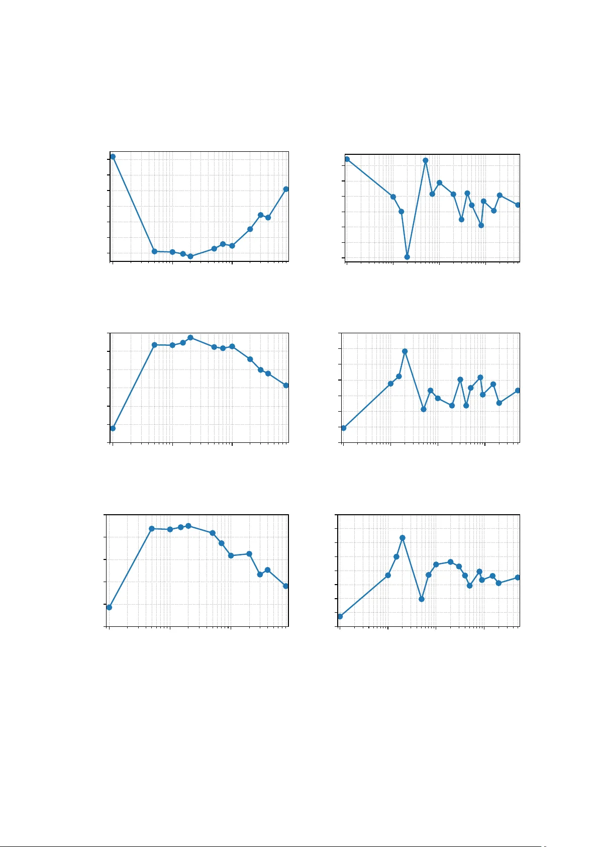
Less is More: Con v ergence Beneﬁts of F ew er Data W eigh t Up dates o v er Longer Horizon Rudra jit Das 1 , Neel P atel 2 , Meisam Raza viy ayn 1,3 , and V ahab Mirrokni 1 1 Go ogle Researc h, 2 EPFL, 3 Univ ersity of Southern California {dasrudrajit, razaviyayn, mirrokni}@google.com, neel.patel@epfl.ch Abstract Data mixing—the strategic reweigh ting of training domains—is a critical comp onen t in training robust mac hine learning mo dels. This problem is naturally formulated as a bilev el optimization task, where the outer lo op optimizes domain w eights to minimize v alidation loss, and the inner lo op optimizes mo del parameters to minimize the weigh ted training loss. Classical bilev el optimization relies on hypergradients, whic h theoretically require the inner optimization to reach con vergence. How ever, due to computational constraints, state-of-the- art metho ds use a ﬁnite, often small, n um b er of inner up date steps b efore up dating the w eights. The theoretical implications of this approximation are not w ell understoo d. In this w ork, w e rigorously analyze the conv ergence b ehavior of data mixing with a ﬁnite num b er of inner steps T . W e pro ve that the “greedy” practical approach of using T = 1 can fail ev en in a simple quadratic example. Under a ﬁxed parameter update budget N and assuming the p er-domain losses are strongly conv ex, w e sho w that the optimal T scales as Θ( log N ) (resp., Θ( √ N log N ) ) for the data mixing problem with access to full (resp., stochastic) gradien ts. W e complemen t our theoretical results with proof-of-concept exp eriments. 1 In tro duction The performance of mo dern machine learning mo dels dep ends heavily on the comp osition of their (pre-)training data Sam basiv an et al. (2021); Whang et al. (2023). In particular, as mo dern foundation models are trained on mixtures of diverse domains (ranging from high-quality co de and textbo oks to noisy w eb scrapes) determining the optimal contribution of each domain, known as data mixing , has b ecome a crucial challenge Brown et al. (2020); T ouvron et al. (2023); Raﬀel et al. (2020); Gao et al. (2020). Historically , data mixtures w ere determined via manual heuristics. F or instance, GPT-3 and P aLM utilized man ual upsampling of “high-qualit y” sources Chowdhery et al. (2023); Bro wn et al. (2020). More recen tly , this has b een formalized into data mixing la ws Y e et al. (2024); Liu et al. (2025). The data mixing problem is naturally cast as a bilev el optimization problem Sinha et al. (2017). The outer lo op seeks to ﬁnd a weigh ting vector w for the training domains that minimizes a v alidation loss L V (represen ting the do wnstream p erformance measured using a high-quality reference set), while the inner lo op minimizes the weigh ted training loss L T with resp ect to the mo del parameters θ F ranceschi et al. (2018); F an et al. (2023). While mathematically elegant, the application of bilev el optimization to data mixing for LLMs faces a severe computational b ottleneck: calculating the exact gradient with resp ect to w —the hyp er gr adient —requires diﬀeren tiating through the en tire training tra jectory of θ (whic h evolv es as a function of w ) un til conv ergence, but this is intractable for large mo dels. T o mak e this feasible, sev eral online mixing metho ds such as DoGE F an et al. (2023) and PIKE Li et al. (2025), as w ell as earlier meta-learning approaches (Ren et al., 2018; Sh u et al., 2019), adopt a “greedy" heuristic. They p erform a single step or very few steps of model parameter up dates b efore 1 up dating the data weigh ts, prioritizing computational eﬃciency ov er h yp ergradien t accuracy . W e refer to the n umber of parameter up dates per weigh t up date as the lo okahe ad horizon , and denote it by T . This reliance on greedy approximations ignites a critical theoretical contro v ersy centered on short-horizon bias (W u et al., 2018). Seminal w orks in meta-learning suggest that truncating the inner optimization lo op to a negligible horizon introduces systematic errors, often leading the meta-learner to adopt my opic strategies—suc h as artiﬁcially suppressing learning rates—to minimize immediate volatilit y rather than maximizing long-term generalization (Shaban et al., 2019). Despite the empirical adoption of greedy mixing metho ds, the theoretical implications of this bias in the simplex-constrained domain of data mixing remain underexplored. Do es the prev alent T = Θ(1) heuristic ﬁnd the optimal mixture, or do es it succum b to truncation bias? In this w ork, we rigorously analyze the conv ergence b ehavior of data mixing as a function of the lo ok ahead horizon T . W e challenge the prev ailing “greedy” heuristic, demonstrating that the strategy of frequen t weigh t up dates with short horizons is systematically biased. W e establish a “ less is mor e ” principle: under a ﬁxed total budget of parameter up dates, it is prov ably better to up date data w eights less fr e quently but with a longer lo okahe ad horizon . Our main contributions are: “Greedy” Approach F ails: W e theoretically sho w that the greedy approac h of using T = 1 in data mixing is not merely noisy but systematically biased. In a simple quadratic example, it can cause data w eights to con verge to sub-optimal v alues, failing to identify the correct mixture (Section 5). Optimal Horizon Scaling: W e derive the optimal scaling la ws for the lo ok ahead horizon T (i.e., n umber of parameter updates p er weigh t update) under a ﬁxed parameter up date budget N = K T , where K is the total n umber of weigh t up dates. Sp eciﬁcally , in the strongly conv ex case, w e prov e that the optimal T scales as Θ( log N ) and Θ( √ N log N ) in the deterministic and sto c hastic settings, resp ectiv ely , contrasting sharply with the Θ(1) horizon commonly used in practice (Section 6). W e corroborate our theoretical ﬁndings with pro of-of-concept experiments whic h show that moderate v alues of T (sublinear in N ) lead to the b est p erformance in practice (Section 7). 2 Related W ork Static Heuristics and Scaling La ws. Historically , data mixtures were determined via man ual heuristics, suc h as upsampling high-quality domains suc h as Wikip edia (Chowdhery et al., 2023). Recen t work has formalized this into data mixing laws (Y e et al., 2024), which ﬁt p ow er-la w regression mo dels on small-scale training runs to predict the loss of larger mo dels. Metho ds lik e UniMax (Ch ung et al., 2024) prop ose maximizing div ersity under ep o ching constraints. While principled, these metho ds are static; they freeze the mixture weigh ts prior to training and cannot adapt to the mo del’s evolving curriculum needs (Bengio et al., 2009). Oﬄine Pro xy-Based Optimization. T o in tro duce data-driven adaptability without the cost of online updates, several metho ds utilize pro xy mo dels (Ren et al., 2018; Sh u et al., 2019). DoReMi (Xie et al., 2023) form ulates data mixing as a distributionally robust optimization (DRO) problem (Sagaw a et al., 2020; Kuhn et al., 2025), training a small pro xy mo del to minimize w orst-case excess loss relative to a reference mo del. RegMix (Liu et al., 2024) treats mixture selection as a regression problem, ﬁtting high-degree p olynomials to map mixture weigh ts to v alidation loss via extensiv e random sampling. While eﬀectiv e, these metho ds incur signiﬁcant pre-computation o verhead and suﬀer from a gap b etw een proxy and target mo del dynamics. 2 Online Bilevel Optimization. The most adaptive paradigm integrates w eight optimiza- tion directly in to the training lo op. Early “learning to w eight” approac hes used auxiliary net works to predict sample w eights (Jiang et al., 2018; Shu et al., 2019), but these struggle to scale to LLMs. Current state-of-the-art methods fo cus on eﬃcient domain-lev el reweigh ting. DoGE (F an et al., 2023) estimates domain w eights b y computing a “generalization gain” via the dot pro duct of v alidation and training gradients. PIKE (Li et al., 2025) extends this to m ulti-task learning b y minimizing gradient conﬂicts. TIKMIX (W ang et al., 2025b) and T ANDEM (W ang et al., 2025a) represen t the new est wa ve of dynamic mixing. Crucially , to main tain eﬃciency , these metho ds rely on the “greedy” approac h ( T = 1 ), up dating w eigh ts based on immediate gradient feedbac k. Theoretical F oundations: T runcation Bias vs. Unrolling. The theoretical v alidity of truncating the inner optimization lo op is a sub ject of in tense scrutin y . W u et al. (2018) iden tiﬁed that short-horizon unrolling in tro duces systematic bias, while Shaban et al. (2019) pro ved that exact conv ergence requires the horizon to scale logarithmically with precision. Con- v ersely , single-lo op metho ds (Ji et al., 2021) argue con vergence is p ossible under strict time-scale separation, though this condition is rarely met in standard pre-training. Alternativ e approaches include Implicit Diﬀeren tiation (Lorraine et al., 2020; Blondel et al., 2022), whic h approximates the in verse Hessian via Neumann series (Grazzi et al., 2020). How ever, recent analysis on the “curse of unrolling” (Scieur et al., 2022) suggests that unrolled diﬀerentiation can suﬀer from n umerical instability o ver long horizons. Our work uniﬁes these p ersp ectives for data mixing, pro viding a rigorous analysis of the “sw eet sp ot” for T that minimizes b oth optimization error and truncation bias. 3 Notation and Preliminaries W e denote v ectors and matrices b y b old fon t sym b ols. F or a natural n umber n ∈ N , w e denote the set { 1 , . . . , n } b y [ n ] . F or a vector v , w e denote its i th co ordinate by v ( i ) and its ℓ p norm by ∥ v ∥ p . A vector v = [ v (1) , . . . , v ( n ) ] is said to b elong to the n -dimensional simplex ∆ n if P n i =1 v ( i ) = 1 and v ( i ) ≥ 0 ∀ i ∈ [ n ] . F or a matrix M , w e denote its operator norm b y ∥ M ∥ op . A function f ( x ) : R d − → R is said to be G -Lipsc hitz if sup x ∈ R d ∥∇ f ( x ) ∥ 2 ≤ G , L -smo oth if ∥∇ f ( y ) − ∇ f ( x ) ∥ 2 ≤ L ∥ y − x ∥ 2 for all x , y ∈ R d , and µ -strongly-con vex if f ( y ) ≥ f ( x ) + ⟨∇ f ( x ) , y − x ⟩ + µ 2 ∥ y − x ∥ 2 2 for all x , y ∈ R d . 4 Problem F orm ulation In pre-training large foundation mo dels, w e are t ypically given access to m div erse training domains (e.g., Wikip edia, GitHub, CommonCra wl), each asso ciated with a loss function ℓ i ( i ∈ [ m ] ). The goal is not simply to minimize the av erage loss on these domains, but to minimize the loss on a v alidation set (or “reference” distribution) L V , whic h serves as a pro xy for do wnstream capabilit y . T o that end, a weigh ted loss o ver the training domains can b e minimized, where the weigh ts should b e c hosen so as to minimize the v alidation loss as m uch as p ossible. This creates a hierarchical dep endency: w e w ant to ﬁnd the mixture w eights w ∈ ∆ m that pro duces a mo del θ ∗ ( w ) whic h p erforms the b est on L V . This is the canonical bilevel optimization form ulation (F rancesc hi et al., 2018; Grazzi et al., 2020): min w ∈ ∆ m F ( w ) := L V ( θ ∗ ( w )) s.t. θ ∗ ( w ) ∈ arg min θ L T ( θ , w ) := m X i =1 w ( i ) ℓ i ( θ ) . (1) 3 Algorithm 1 Data Mixing Input: Initialization for mo del parameters θ 0 , initialization for mixture w eights w 0 , parameter up date step-size η , weigh t up date step-size α , num b er of rounds K , num b er of parameter up dates p er round / “horizon” T . Set θ 0 , 0 = θ 0 . for k ∈ { 0 , . . . , K − 1 } do for t ∈ { 0 , . . . , T − 1 } do Up date θ k,t +1 = θ k,t − η ∇ θ L T ( θ k,t , w k ) . // Inner parameter update end for F or j ∈ [ m ] , up date w ( j ) k +1 = w ( j ) k exp  − α ¯ g ( j ) k,T  P m s =1 w ( s ) k exp  − α ¯ g ( s ) k,T  , with ¯ g ( j ) k,T := ∂ L V ( θ k,T ) ∂ w ( j ) k . // Outer weight update Set θ k +1 , 0 = θ k,T . end for Return θ K, 0 and w K . Note that for F ( w ) to b e w ell-deﬁned, we need to uniquely sp ecify θ ∗ ( w ) as one particular optim um of L T ( θ , w ) if it has m ultiple optima. F or example, this could b e the optimum closest to the initialization. The hypergradient c hallenge. T o optimize w via ﬁrst-order methods, we need the hyp er gr a- dient ∇ F ( w ) . Using the Implicit F unction Theorem (IFT), the j th ( j ∈ [ m ] ) coordinate of this is giv en by: ∇ F ( w ) ( j ) = − D ∇ θ L V  θ ∗  , ∇ 2 θ L T  θ ∗ , w  − 1 ∇ ℓ j  θ ∗  E , (2) where for brevity θ ∗ denotes θ ∗ ( w ) . 1 Unfortunately , computing the exact quan tity in Eq. 2 is intractable for tw o reasons: (1) for every single up date of w , it requires training θ to full con vergence ( θ ∗ ), and (2) it requires inv erting the massiv e Hessian matrix at θ ∗ . So w e fo cus on a more practical unr ol le d algorithm , where the inner optimization w.r.t θ is appro ximated by a few steps, sa y T , of gradien t descen t, which is then used to appro ximate the hypergradient. 2 W e formally describ e this unrolled algorithm in Algorithm 1. It can b e viewed as a coupled system where eac h “round” consists of T inner parameter up dates follo wed by one outer w eight up date. In Algorithm 1, θ k,t denotes the parameter at step t of round k , while w k denotes the w eight v ector in round k . The inner parameter up date rule θ k,t +1 = θ k,t − η ∇ θ L T ( θ k,t , w k ) , (3) is standard gradient descent with constant step-size η . After T parameter up date steps, w e compute the gradien t of the v alidation loss at θ k,T with respect to the current weigh ts w k (i.e., ∂ L V ( θ k,T ) ∂ w k ) to up date them. Speciﬁcally , for updating the weigh ts, w e perform mirror-descent Bub ec k et al. (2015) with the negative entrop y function as the Bregman divergence and constant step-size α . Note that if T → ∞ , then we will get the exact hypergradient in Equation (2). Unfortunately , as T increases, k eeping trac k of ∂ L V ( θ k,T ) ∂ w k exactly b ecomes c hallenging. T o see this, note that the 1 See Theorem C.3 for a quick pro of of this result. 2 Note that T → ∞ would lead to con vergence to θ ∗ . 4 j th co ordinate of ∂ L V ( θ k,T ) ∂ w k , i.e., ∂ L V ( θ k,T ) ∂ w ( j ) k = * ∇ θ L V ( θ k,T ) , ∂ θ k,T ∂ w ( j ) k + , (4) using the chain rule. Now, ∂ θ k,T ∂ w ( j ) k is not straightforw ard to compute. The follo wing prop osition describ es ho w this quantit y can b e computed recursively . Prop osition 4.1. F or t ≥ 0 , ∂ θ k,t ∂ w ( j ) k evolves as: ∂ θ k,t ∂ w ( j ) k =  I − η ∇ 2 θ L T  θ k,t − 1 , w k   ∂ θ k,t − 1 ∂ w ( j ) k − η ∇ ℓ j  θ k,t − 1  , (5) with initial c ondition ∂ θ k, 0 ∂ w ( j ) k =  0 . The pro of of Theorem 4.1 is in Section B. This recursion rev eals that the inﬂuence of a w eight w ( j ) k accum ulates ov er the tra jectory , decay ed by a matrix dep ending on the Hessian of the weigh ted training loss ov er the tra jectory . Th us, the exact computation of ∂ L V ( θ k,T ) ∂ w ( j ) k b ecomes infeasible as T increases. As a result, an extreme version of Alg. 1 is used in man y practical algorithms. F or example, DoGE F an et al. (2023) and PIKE Li et al. (2025) propose a “greedy” approac h b y setting T = 1 . How ever, using T = 1 or a small v alue of T migh t yield a p o or appro ximation of the h yp ergradient, which might b e detrimen tal to conv ergence. Indeed, in Section 5, we show that T = 1 leads to sub optimal p erformance in a simple example inv olving quadratic losses. Our main fo cus. Motiv ated by this conundrum, we seek to rigorously analyze the impact of the horizon T on conv ergence. More imp ortantly , given a ﬁxed parameter up date budget N = K T , w e wish to quantify the optimal v alue of T as a function of N that results in the b est con vergence b ound. W e present this analysis in Section 6 for a more general and practical version of Algorithm 1. Our k ey insight. W e show that T = Θ(1) (here, Θ( · ) is with resp ect to the total parameter up date budget N ) is sub optimal and a larger v alue of T leads to the b est conv ergence b ound; see T able 1 for a summary of our results. In other w ords, we show that making few er w eight up dates with a go o d appro ximation of the hypergradient (obtained with a large T ) leads to b etter p erformance than making more w eight updates with a p o or approximation of the h yp ergradient (obtained with T = Θ(1) ), i.e., less is mor e . T able 1: Optimal horizon T (leading to best con vergence b ound) as a function of the total parameter up date budget N , when the p er-domain losses are strongly conv ex. In the deterministic (resp., stochastic) case, we hav e access to full (resp., sto chastic) gradients. Setting Optimal Horizon T Deterministic (Sec. 6.2) Θ  log N  Stochastic (Sec. 6.3) Θ  √ N log N  It is w orth clarifying here that we are not pitching Algorithm 1 as a nov el algorithm; rather, our main contribution is theoretically deriving the optimal v alue of T in it. 5 5 Motiv ating Example and Initial Insights Here w e analyze a 1-dimensional quadratic setting where the “greedy” approac h of using T = 1 fails. Quadratic example. Consider a scalar parameter θ and weigh t w ∈ [0 , 1] controlling tw o training domains: L T ( θ , w ) = w  θ 2 2  + (1 − w )  ( θ − 1) 2 2  , L V ( θ ) = θ 2 2 . Here, the v alidation domain is iden tical to the ﬁrst training domain. Thus, the optimal weigh t is clearly w ∗ = 1 , whic h yields θ ∗ = 0 . F or this example, the theorem b elow shows that the greedy approac h of setting T = 1 completely fails when starting far aw ay from the optimum θ ∗ = 0 , while a larger v alue of T do es not suﬀer from this problem. Theorem 5.1 (Informal: F ailure of Greedy Approach) . Supp ose we run Algorithm 1 starting fr om w 0 = 0 . 5 and θ 0 = − R , with R > 0 b eing suﬃciently lar ge. L et the total p ar ameter up date budget b e N ( = K T ). • Case 1 ( T = 1 ): The ﬁnal weight iter ate w K c onver ges to 0 , while the optimal weight is 1 . • Case 2 ( T ≫ 1 ): If T sc ales as Θ( log R ) , the ﬁnal weight iter ate w K c an b e made to c onver ge to a value arbitr arily close to the optimal value 1 . The formal statement of Theorem 5.1 and its pro of are relegated to Section A. This result sho ws that T = 1 is problematic even in a simple quadratic example, and conv erging to the optimal w eight requires making use of a larger horizon T . At a high lev el, in the T = 1 case, the algorithm up dates weigh ts based on immediate but “misleading” v alidation loss improv emen t. T o see this, notice that at θ 0 = − R , the gradien t of the second domain’s loss is steep er and lo cally reduces v alidation loss faster, incorrectly signaling that w should decrease. In contrast, when using a larger v alue of T , the algorithm do es not suﬀer from this short-term bias and receives the correct signal that w should increase to align with the v alidation loss. Note that under a constant budget N = K T , as T increases, the num b er of w eigh t up dates K decreases. Given that w e show ed T ≫ 1 is b etter than T = 1 , w e also sho wed that making few er weigh t up dates with a relativ ely precise h yp ergradien t is b etter than greedily making more w eight up dates with an erroneous h yp ergradient, i.e., less is mor e ! With these insigh ts in mind, we will mov e on to Section 6 which presents a muc h more general analysis of this phenomenon. 6 Main Results: Less is More T o formally understand the role of the horizon T , this section provides conv ergence b ounds for a more general and practical version of Algorithm 1, assuming the p er-domain losses are strongly-con vex and smo oth. 6.1 Practical V ersion of Algorithm 1 Using Approximate Hessian Let us ﬁrst describ e the computationally-practical v ersion of Algorithm 1 that we analyze. Recall that to up date the w eights, we need to compute ∂ L V ( θ k,T ) ∂ w ( j ) k ( j ∈ [ m ] ) which by the chain rule is equal to  ∇ θ L V ( θ k,T ) , ∂ θ k,T ∂ w ( j ) k  (see Eq. (4) ). As discussed, ∂ θ k,T ∂ w ( j ) k can be computed recursively with the following recursive up date rule from Theorem 4.1: ∂ θ k,t ∂ w ( j ) k =  I − η H k,t − 1  ∂ θ k,t − 1 ∂ w ( j ) k − η ∇ ℓ j  θ k,t − 1  , 6 where H k,t − 1 := ∇ 2 θ L T  θ k,t − 1 , w k  and initial condition ∂ θ k, 0 ∂ w ( j ) k =  0 . Since the computation of the Hessian H k,t at ev ery step is costly , w e consider using a single approximate Hessian H k for the en tire round k . Sp eciﬁcally , we assume access to a Hessian approximator H that tak es as input w k and returns an approximate Hessian H k = H ( w k ) . 3 Under this sc heme, let the approximation to n ∂ θ k,t ∂ w ( j ) k o t b e denoted b y  − η u ( j ) k,t  t , whic h has the follo wing simpler recursiv e up date: u ( j ) k,t =  I − η H k  u ( j ) k,t − 1 + ∇ ℓ j  θ k,t − 1  , (6) with u ( j ) k, 0 =  0 . Unfolding the recursion in Eq. (6), w e get: u ( j ) k,T = T − 1 X i =0  I − η H k  T − 1 − i ∇ ℓ j  θ k,i  . (7) Let us denote the approximation for ∂ L V ( θ k,T ) ∂ w ( j ) k that w e will obtain b y approximating ∂ θ k,T ∂ w ( j ) k with − η u ( j ) k,T b y g ( j ) k,T ; so, g k,T = h g (1) k,T , . . . , g ( m ) k,T i ⊤ is our appro ximate hypergradient. Plugging in Equation (7) in to Equation (4) and dropping the subscript θ in ∇ θ L V ( θ k,T ) henceforth, w e get: g ( j ) k,T = − η T − 1 X i =0 D ∇L V ( θ k,T ) ,  I − η H k  T − 1 − i ∇ ℓ j  θ k,i  E . (8) The corresponding up date rule for w k is: w ( j ) k +1 = w ( j ) k exp  − αg ( j ) k,T  P m s =1 w ( s ) k exp  − αg ( s ) k,T  . (9) W e concretely present this practical ver sion in Algorithm 2. 6.2 Con vergence Result for Algorithm 2 No w we will provide a con v ergence result for Algorithm 2 under the following assumptions. Assumption 6.1 ( Domain losses ) . Each ℓ j ( θ ) ( j ∈ [ m ] ) is G -Lipsc hitz, L -smo oth, and µ -strongly-con vex. Note that when the ℓ j ’s are strongly con vex, θ ∗ ( w ) is unique and F ( w ) in Eq. (1) is unam biguously deﬁned. Assumption 6.2 ( V alidation loss ) . L V ( θ ) is G V -Lipsc hitz and L V -smo oth. Assumption 6.3 ( Hessian approximation ) . F or w ∈ ∆ m , supp ose H ∗ ( w ) := ∇ 2 θ L T  θ ∗ ( w ) , w  is the Hessian at the optimum of the weigh ted training loss with weigh t w , and H ( w ) is the appro ximate Hessian returned by our Hessian approximator (recall that we denoted this by H k for round k in Section 6.1). Then, H ( w ) is PSD with b µ I ⪯ H ( w ) ⪯ b L I and ∥ H ( w ) − H ∗ ( w ) ∥ op ≤ δ ∀ w ∈ ∆ m . W e are now ready to present our result for Algorithm 2. 3 W e discuss a practical choice of H k in Section E. 7 Algorithm 2 Data Mixing with Approximate Hessian 1: Input: Initialization for mo del parameters θ 0 , initialization for mixture w eights w 0 , parame- ter update step-size η , w eight up date step-size α , n umber of rounds K , n umber of parameter up dates p er round / “horizon” T , and Hessian approximator H for weigh ted training loss. 2: Set θ 0 , 0 = θ 0 . 3: for k ∈ { 0 , . . . , K − 1 } do 4: Obtain Hessian approximation H k = H ( w k ) . 5: Set u ( j ) k, 0 =  0 for j ∈ [ m ] . 6: for t ∈ { 0 , . . . , T − 1 } do 7: Up date θ k,t +1 = θ k,t − η ∇ θ L T ( θ k,t , w k ) . // Inner parameter update 8: for j ∈ { 1 , . . . , m } do 9: Up date u ( j ) k,t +1 =  I − η H k  u ( j ) k,t + ∇ ℓ j  θ k,t  10: end for 11: end for 12: F or j ∈ [ m ] , up date w ( j ) k +1 = w ( j ) k exp  − αg ( j ) k,T  P m s =1 w ( s ) k exp  − αg ( s ) k,T  , where g ( j ) k,T := − η D ∇L V ( θ k,T ) , u ( j ) k,T E . // Outer weight update 13: Set θ k +1 , 0 = θ k,T . 14: end for 15: Return { θ k, 0 } K k =0 and { w k } K k =0 . Theorem 6.4. Supp ose Assumptions 6.1, 6.2 and 6.3 hold, F ( w ) = L V  θ ∗ ( w )  is c onvex (in w ), and F ∗ := min w ∈ ∆ m F ( w ) . L et N = K T denote the total p ar ameter up date budget. Supp ose our initialization is w 0 = 1 m 1 m . Then, ∃ α such that for any η < min  1 b L , µ L 2  and T ≥  log 4 η µ  , we have the fol lowing guar ante e for Algorithm 2: F ( w K ) − F ∗ ≤ c 1 √ T √ N | {z } (I) +  1 − η µ 2  T − 1 ( c 2 η T + c 3 ) | {z } (II) + c 4 δ |{z} (II I) , (10) wher e w K := 1 K P K − 1 k =0 w k , and { c i } 4 i =1 ar e c onstants indep endent of T and N . In Equation (10) , term (I) is the optimization err or , term (II) is the ﬁnite horizon bias , while term (I I I) is the irr e ducible Hessian appr oximation err or . The detailed version and pro of of Theorem 6.4 are presented in Section C. T erms (I) and (I I) in Eq. (10) are reducible by increasing N and choosing T appropriately (as a function of N ). How ever, term (I I I) is indep endent of N and T , and cannot be reduced. This is the Hessian appro ximation cost, which dep ends on the qualit y of the appro ximator. Reducible error. The reducible error ((I) + (I I)) in Equation (10) is asso ciated with a tradeoﬀ with respect to the v alue of T . Sp eciﬁcally , the optimization error (I) increases with T (or as as K = N /T decreases), while the horizon bias (I I) decays with T asymptotically . As we discuss and show in the detailed v ersion of Theorem 6.4 (Theorem C.1), the reducible error is minimized b y choosing T = Θ(log N ) . 4 (11) 4 Note that the Θ( · ) used here and subsequently is w.r.t. N . Also, η is chosen to be a constant indep endent of N for this result. 8 R emark 6.5 . The reducible error is minimized by setting T = Θ( log N ) . This establishes that T = Θ(1) is sub optimal and making few er weigh t up dates with the horizon growing lo garithmic al ly with the total parameter update budget is b etter, i.e., less is more ! Tigh tness. Since F ( w ) is assumed to b e con vex in Theorem 6.4, we ha ve a low er b ound of Ω  1 √ N  in the worst case Nestero v (2013). Note that b y c ho osing T = Θ( log N ) , the reducible error in ((I) + (II)) in Eq. (10) b ecomes e O  1 √ N  (where e O ( · ) hides p oly-log factors). Thus, our upp er b ound in Theorem 6.4 with T = Θ( log N ) matches the lo wer b ound (ignoring p oly-log factors). This establishes that T = Θ(log N ) is indeed the optimal choice in this setting. 6.3 Extension to the Sto c hastic Case Here, w e consider a more practical version of Algorithm 2, where for each domain loss ℓ j ( · ) and the v alidation loss L V ( · ) , w e hav e access to unbiased sto chastic gradien ts e ∇ ℓ j ( · ) and e ∇L V ( · ) instead of the actual gradients ∇ ℓ j ( · ) and ∇L V ( · ) . In this case, we hav e three c hanges in Algorithm 2. First, line 7 (inner parameter up date) b ecomes θ k,t +1 = θ k,t − η e ∇ θ L T ( θ k,t , w k ) , where e ∇ θ L T ( θ k,t , w k ) = P m j =1 w ( j ) k e ∇ ℓ j  θ k,t  . Second, line 9 c hanges to e u ( j ) k,t +1 =  I − η H k  e u ( j ) k,t + e ∇ ℓ j  θ k,t  , with e u ( j ) k, 0 =  0 . Finally , line 12 (outer weigh t up date) b ecomes w ( j ) k +1 = w ( j ) k exp  − α e g ( j ) k  P m s =1 w ( s ) k exp  − α e g ( s ) k  , with e g ( j ) k = − η  e ∇L V ( θ k,T ) , e u ( j ) k,T  . Note that e g k,T = h e g (1) k,T , . . . , e g ( m ) k,T i ⊤ is our appro ximate h yp ergradient here. F or full clarity , we write down the resultant algorithm in the sto c hastic case in Algorithm 3. W e make the following standard assumptions on the stochastic gradients. Assumption 6.6 ( Sto chastic gradien ts ) . Suppose ζ denotes the source of randomness in the sto c hastic gradients. The stochastic gradients: 1. are un biased, i.e., E ζ  e ∇ ℓ j ( θ )  = ∇ ℓ j ( θ ) and E ζ  e ∇L V ( θ )  = ∇L V ( θ ) , ∀ θ . 2. ha ve b ounded v ariance, i.e., E ζ  ∥ e ∇ ℓ j ( θ ) −∇ ℓ j ( θ ) ∥ 2 2  ≤ σ 2 and E ζ  ∥ e ∇L V ( θ ) −∇L V ( θ ) ∥ 2 2  ≤ σ 2 , ∀ θ . W e are now ready to present our con v ergence result for the algorithm in the sto chastic case (Algorithm 3). Theorem 6.7 ( Sto chastic case ) . Supp ose Assumptions 6.1, 6.2, 6.3 and 6.6 hold, F ( w ) = L V  θ ∗ ( w )  is c onvex (in w ), and F ∗ := min w ∈ ∆ m F ( w ) . L et N = K T denote the total p ar ameter up date budget. Supp ose our initialization is w 0 = 1 m 1 m . Then, ∃ α and η such that for any T ≥ Ω(1) (w.r.t. N ), we have the fol lowing guar ante e for A lgorithm 3: E  F ( w K )  − F ∗ ≤ O  √ T √ N  | {z } (I) + O  √ log T √ T  | {z } (II) + O ( δ ) | {z } (II I) , (12) 9 Algorithm 3 Data Mixing with Approximate Hessian and Sto chastic Gradients 1: Input: Initialization for mo del parameters θ 0 , initialization for mixture w eights w 0 , parame- ter update step-size η , w eight up date step-size α , n umber of rounds K , n umber of parameter up dates p er round / “horizon” T , and Hessian appro ximator H for the w eighted training loss. 2: Set θ 0 , 0 = θ 0 . 3: for k ∈ { 0 , . . . , K − 1 } do 4: Obtain Hessian approximation H k = H ( w k ) . 5: Set e u ( j ) k, 0 =  0 for j ∈ [ m ] . 6: for t ∈ { 0 , . . . , T − 1 } do 7: Up date θ k,t +1 = θ k,t − η  P m j =1 w ( j ) k e ∇ ℓ j  θ k,t   . // Inner parameter update 8: for j ∈ { 1 , . . . , m } do 9: Up date e u ( j ) k,t +1 =  I − η H k  e u ( j ) k,t + e ∇ ℓ j  θ k,t  . 10: end for 11: end for 12: F or j ∈ [ m ] , up date w ( j ) k +1 = w ( j ) k exp  − α e g ( j ) k,T  P m s =1 w ( s ) k exp  − α e g ( s ) k,T  , where e g ( j ) k,T := − η D e ∇L V ( θ k,T ) , e u ( j ) k,T E . // Outer weight update 13: Set θ k +1 , 0 = θ k,T . 14: end for 15: Return { θ k, 0 } K k =0 and { w k } K k =0 . wher e w K := 1 K P K − 1 k =0 w k . 5 In Equation (12) , term (I) is the optimization err or , term (I I) is the ﬁnite horizon bias , while term (I I I) is the irr e ducible Hessian appr oximation err or . The detailed version and proof of Theorem 6.7 are presen ted in Section D. Just like Theo- rem 6.4, there are reducible error terms (I) and (I I), and an irreducible error term (I I I), which is the Hessian approximation cost. Reducible error. Similar to Theorem 6.4, the optimization error (I) increases with T (or as as K = N /T decreases), while the horizon bias (I I) decays with T asymptotically . How ev er, in this case, the deca y in the horizon bias is m uc h slow er (as a function of T ) than in Theorem 6.4; this is due to the use of sto chastic gradients here. As w e discuss and sho w in the detailed version of Theorem 6.7 (Theorem D.1), the reducible error ((I) + (I I)) is minimized by choosing T = Θ  p N log N  . (13) R emark 6.8 . In the sto chastic case, the reducible error is minimized by setting T = Θ  √ N log N  whic h is signiﬁcan tly larger than Θ(1) as w ell as the optimal v alue of Θ( log N ) in the deterministic case (Theorem 6.5). 6.4 Pro of Sk etc h: Bounding the Hyp ergradien t Error The core of our analysis lies in b ounding the deviation of the appro ximate h yp ergradi- en t g k,T (or its sto chastic coun terpart e g k,T ) from the true hypergradient ∇ F ( w k ) ; the rest of 5 The expectation in Equation (12) is w.r.t. the randomness of the algorithm due to use of sto chastic gradients. 10 the analysis is based on standard results for mirror descent. Recall that the true h yp ergradient is giv en by the Implicit F unction Theorem as ∇ F ( w ) ( j ) = −  ∇ θ L V  θ ∗  , ∇ 2 θ L T  θ ∗ , w  − 1 ∇ ℓ j  θ ∗  , where θ ∗ denotes θ ∗ ( w ) (for brevity). Our analysis decomp oses this error into tw o primary sources: the ﬁnite-horizon bias from truncating the inner optimization, and the appro xima- tion error from replacing the exact in verse Hessian at the optim um with a truncated Neumann series o ver the optimization tra jectory using the appro ximate Hessian. Deterministic setting (Theorem 6.4). Let H ∗ k := ∇ 2 θ L T  θ ∗ k , w k  . Here the analysis boils do wn to b ounding ∥∇ F ( w k ) − g k,T ∥ ∞ , and this is done by expressing the inv erse Hessian ( H ∗ k ) − 1 in ∇ F ( w k ) as an inﬁnite Neumann series η P ∞ i =0  I − η H ∗ k  i . Our estimated hypergradient g k,T appro ximates this b y using the approximate Hessian H k instead of H ∗ k , truncating the sum to T terms, and ev aluating gradien ts along the ﬁnite tra jectory { θ k,t } T t =0 rather than at the optimum θ ∗ k . W e split the error into tw o parts: 1. T ail error. This is the error from ignoring terms i ≥ T in the Neumann series. Due to strong conv exity of the p er-domain losses,  I − η H ∗ k  is a contractiv e op erator with sp ectral radius b ounded b y (1 − η µ ) . As a result, this tail error deca ys exp onentially as (1 − η µ ) T . 2. T ra jectory error. This is the error accum ulating from ev aluating gradients at { θ k,t } T t =0 instead of θ ∗ k as w ell as from the use of approximate Hessian instead of exact Hessian. Since gradien t descent on strongly-con vex functions con verges linearly , ∥ θ k,t − θ ∗ k ∥ 2 deca ys as  1 − O ( η µ )  t . Using this fact together with the Lipsc hitzness and smo othness of the per-domain and v alidation losses, it can b e shown that this error is bounded b y O  η T  1 − O ( η µ )  T  + O ( δ ) , where the last term is due to the Hessian approximation and is irreducible. Com bining these tw o errors, the total h yp ergradient error is b ounded by O  η T  1 − O ( η µ )  T  + O ( δ ) , where δ is the irreducible error from the Hessian approximator. This near-exp onential deca y in the hypergradient error driv es the optimal c hoice of T = Θ(log N ) . Sto c hastic setting (Theorem 6.7). In the sto chastic case, the high-level idea is similar to the determi nistic case, but the analysis is more in volv ed and tric ky due to the use of sto c hastic gradients. After taking conditional exp ectations judiciously , the decomp ositions are similar to the deterministic case. The k ey diﬀerence here compared to the deterministic case is that the θ k,t ’s do not con verge to θ ∗ k linearly; sp eciﬁcally , here we ha ve E    θ k,T − θ ∗ k   2  ≤ O  1 − O ( η µ )  T  + O ( √ η σ ) . The noise v ariance term at the end O ( √ η σ ) turns out to b e the dominan t term in the reducible 6 part of the exp ected hypergradient error; the other terms deca y as O  η T  1 − O ( η µ )  T  just lik e the deterministic case. By c ho osing η = O ( log T µT ) , the reducible part of the exp ected hypergradient error is minimized and it turns out to b e O ( √ log T √ T ) . This decay rate is muc h slow er than the deterministic case (where it was near-exp onential asymptotically), and this necessitates a muc h larger optimal horizon T = Θ( √ N log N ) . Analysis without assuming conv exit y . In all of our previous results, w e assumed F ( w ) to b e conv ex. Even in the case when F ( w ) is smo oth non-con v ex, the crux of the analysis lies in b ounding the deviation of the approximate hypergradient from the true hypergradient, and the same analysis that w e ha ve in the con vex case (as discussed in Section 6.4) essentially go es through in this case (assuming the ℓ j ( θ ) ’s are still strongly conv ex). There are no additional imp ortant te chnic al chal lenges compared to the con v ex case; so the exact deriv ation is left for future w ork. 6 The irreducible O ( δ ) term in the deterministic case (due to Hessian appro ximation) sta ys here as well. 11 10 0 10 1 10 2 10 3 T 0.3 0.4 0.5 0.6 val loss N = 1000 (a) V alidation loss vs. T for N = 1000 10 0 10 1 10 2 10 3 T 0.0 0.2 0.4 0.6 0.8 1.0 w 2 N = 1000 (b) w 2 vs. T for N = 1000 10 0 10 1 10 2 10 3 T 0.15 0.20 0.25 0.30 val loss N = 5000 (c) V alidation loss vs. T for N = 5000 10 0 10 1 10 2 10 3 T 0.0 0.2 0.4 0.6 0.8 w 2 N = 5000 (d) w 2 vs. T for N = 5000 Figure 1: V alidation loss and the weigh t of the second domain (most aligned with v alidation data) w 2 as a function of the horizon T , for N = { 1000 , 5000 } . Note that the v alidation loss is lo west and w 2 is highest when T is lar ger than 1 and subline ar in N . 7 Empirical Ev aluation W e design a m ulti-domain training exp erimen t to illustrate ho w increasing the horizon T (i.e., up dating the mixture weigh ts less frequently) leads to better p erformance. Sp eciﬁcally , we consider the following multi-domain data built out of MNIST. Data Domains: W e construct three training domains (for a pretraining setting) from standard MNIST data. Domain (i) is the v anilla domain with standard pre-pro cessing, Domain (ii) is the rotated domain with strong randomly chosen rotation augmen tation, and Domain (iii) is the noisy domain whic h is standard MNIST corrupted with label noise. V alidation data is a ﬁxed rotated v ersion of the MNIST test set, so the rotated domain (Domain (ii)) is the one that b est matc hes the v alidation distribution. W e train a CNN whose arc hitecture we describ e in App endix F. Data Mixing Algorithm: W e consider Algorithm 3 with approximate Hessian H k = γ I , for all k (see Section E). More details ab out the h yp erparameters, etc., are deferred to App endix F. In Figure 1, we show the v alidation loss and the w eight of the second domain (which is the “imp ortan t” domain, most aligned with v alidation data), viz., w 2 , as a function of the horizon T for N = 1000 and N = 5000 . W e discuss the results next. In Figure 2 (Section F), we also plot 12 the v alidation accuracies. Optimal horizon is not small. The p erformance is p o or with a small horizon T (or very frequen t weigh t up dates). With small T , the v alidation loss is high (Figures 1a and 1c), and the corresp onding v alues of w 2 are small (Figures 1b and 1d). This suggests that the hypergradients with small T are inaccurate and misled b y short-horizon bias, underestimating the ev en tual b eneﬁt of allo cating high w eight to an imp ortant domain that may not reduce the loss immediately . As T increases to an intermediate regime , p erformance impro ves substan tially : v alidation loss decreases and w 2 increases, yielding a “sweet sp ot” at moderate horizons. In this regime, the h yp ergradients are muc h more precise and reﬂectiv e of the domain’s actual imp ortance, leading to go o d p erformance. How ever, when T b ecomes to o large, p erformance degrades again b ecause of too few weigh t up dates. Ov erall, this exp erimen t corrob orates our theoretical result that small horizons are sub optimal due to b eing prone to getting misled by short-term spurious signals, while intermediate (in particular, sublinear in N ) horizons do not suﬀer from this issue. Th us, less is mor e ! 8 Conclusion In this work, w e show ed that the prev alen t “greedy” heuristic of frequen t weigh t up dates with short horizons ( T = Θ(1) ) is systematically biased, often conv erging far aw ay from the optimal domain w eights. By deriving rigorous scaling la ws for the horizon, w e established a “less is more” principle, proving that up dating w eigh ts less frequently with a horizon growing sublinearly in the total parameter up date budget signiﬁcantly improv es conv ergence. W e conclude this paper by discussing some limitations and future directions of w ork. Our results in this pap er are under the assumption that the p er-domain losses are strongly conv ex. While this assumption is limiting, a critical challenge in analyzing the general non-conv ex case is that for F ( w ) to b e well-deﬁned in Eq. (1) , θ ∗ ( w ) needs to b e uniquely sp eciﬁed as one of the minimizers of L T ( θ , w ) , and the distance of the iterates from this θ ∗ ( w ) needs to b e b ounded in the pro ofs. It is not clear ho w this can be done, and so, we leav e this analysis for future work. Also, w e would like to conduct exp erimen ts on larger mo dels and datasets in the future. References Agarw al, N., Bullins, B., and Hazan, E. (2017). Second-order sto chastic optimization for machine learning in linear time. Journal of Machine L e arning R ese ar ch , 18(116):1–40. Bengio, Y. (2000). Gradien t-based optimization of hyperparameters. Neur al c omputation , 12(8):1889–1900. Bengio, Y., Louradour, J., Collob ert, R., and W eston, J. (2009). Curriculum learning. In Pr o c e e dings of the 26th annual international c onfer enc e on machine le arning , pages 41–48. Blondel, M., Berthet, Q., Cuturi, M., F rostig, R., Hoy er, S., Llinares-López, F., Pedre gosa, F., and V ert, J.-P . (2022). Eﬃcient and mo dular implicit diﬀerentiation. A dvanc es in neur al information pr o c essing systems , 35:5230–5242. Bonnans, J. F. and Shapiro, A. (2013). Perturb ation analysis of optimization pr oblems . Springer Science & Business Media. Bro wn, T., Mann, B., Ryder, N., Subbiah, M., Kaplan, J. D., Dhariwal, P ., Neelak antan, A., Sh yam, P ., Sastry , G., Askell, A., et al. (2020). Language models are few-shot learners. A dvanc es in neur al information pr o c essing systems , 33:1877–1901. 13 Bub ec k, S. et al. (2015). Con v ex optimization: Algorithms and complexity . F oundations and T r ends ® in Machine L e arning , 8(3-4):231–357. Cho wdhery , A., Narang, S., Devlin, J., Bosma, M., Mishra, G., Rob erts, A., Barham, P ., Chung, H. W., Sutton, C., Gehrmann, S., et al. (2023). P alm: Scaling language modeling with path wa ys. Journal of Machine L e arning R ese ar ch , 24(240):1–113. Ch ung, H. W., Garcia, X., Rob erts, A., T ay , Y., Firat, O., Narang, S., and Constan t, N. (2024). Unimax: F airer and more eﬀective language sampling for large-scale m ultilingual pretraining. In The Eleventh International Confer enc e on L e arning R epr esentations . F an, S., Pagliardini, M., and Jaggi, M. (2023). DOGE: Domain reweigh ting with generalization estimation. In A dvanc es in Neur al Information Pr o c essing Systems (NeurIPS) . F rancesc hi, L., F rasconi, P ., Salzo, S., Grazzi, R., and Pon til, M. (2018). Bilev el programming for h yp erparameter optimization and meta-learning. In International Confer enc e on Machine L e arning (ICML) . Gao, L., Biderman, S., Black, S., Golding, L., Hopp e, T., F oster, C., Phang, J., He, H., Thite, A., Nab eshima, N., et al. (2020). The pile: An 800gb dataset of diverse text for language mo deling. arXiv pr eprint arXiv:2101.00027 . Grazzi, R., F rancesc hi, L., P ontil, M., and Salzo, S. (2020). On the iteration complexity of h yp ergradient computation. In International Confer enc e on Machine L e arning (ICML) . Ji, K., Y ang, J., and Liang, Y. (2021). Bilev el optimization: Con vergence analysis and enhanced design. In International Confer enc e on Machine L e arning (ICML) , pages 4859–4869. Jiang, L., Zhou, Z., Leung, T., Li, L.-J., and F ei-F ei, L. (2018). Men tornet: Learning data-driven curriculum for v ery deep neural net works on corrupted lab els. In International c onfer enc e on machine le arning , pages 2304–2313. PMLR. Kuhn, D., Shaﬁee, S., and Wiesemann, W. (2025). Distributionally robust optimization. A cta Numeric a , 34:579–804. Li, Z., Deng, Y., Zhong, P ., Razaviy ayn, M., and Mirrokni, V. (2025). PIKE: A daptive data mixing for m ulti-task learning under lo w gradien t conﬂicts. In A dvanc es in Neur al Information Pr o c essing Systems (NeurIPS) . Liu, Q., Zheng, X., Muennighoﬀ, N., Zeng, G., Dou, L., P ang, T., Jiang, J., and Lin, M. (2024). Regmix: Data mixture as regression for language mo del pre-training. arXiv pr eprint arXiv:2407.01492 . Liu, Q., Zheng, X., Muennighoﬀ, N., Zeng, G., Dou, L., P ang, T., Jiang, J., and Lin, M. (2025). RegMix: Data mixture as regression for language model pre-training. In International Confer enc e on L e arning R epr esentations (ICLR) . Lorraine, J., Vicol, P ., and Duvenaud, D. (2020). Optimizing millions of hyperparameters by implicit diﬀeren tiation. In International Confer enc e on A rtiﬁcial Intel ligenc e and Statistics (AIST A TS) , pages 1540–1552. Nestero v, Y. (2013). Intr o ductory le ctur es on c onvex optimization: A b asic c ourse , v olume 87. Springer Science & Business Media. Raﬀel, C., Shazeer, N., Rob erts, A., Lee, K., Narang, S., Matena, M., Zhou, Y., Li, W., and Liu, P . J. (2020). Exploring the limits of transfer learning with a uniﬁed text-to-text transformer. Journal of machine le arning r ese ar ch , 21(140):1–67. 14 Ren, M., Zeng, W., Y ang, B., and Urtasun, R. (2018). Learning to reweigh t examples for robust deep learning. In International Confer enc e on Machine L e arning (ICML) . Saga wa, S., Koh, P . W., Hashimoto, T. B., and Liang, P . (2020). Distributionally robust neural net works. In International Confer enc e on L e arning R epr esentations . Sam basiv an, N., Kapania, S., Highﬁll, H., Akrong, D., Paritosh, P ., and Aroy o, L. M. (2021). “ev eryone wan ts to do the mo del work, not the data work”: Data cascades in high-stak es ai. In pr o c e e dings of the 2021 CHI Confer enc e on Human F actors in Computing Systems , pages 1–15. Scieur, D., Gidel, G., Bertrand, Q., and Pedregosa, F. (2022). The curse of unrolling: Rate of diﬀeren tiating through optimization. A dvanc es in Neur al Information Pr o c essing Systems , 35:17133–17145. Shaban, A., Cheng, C.-A., Hatch, N., and Bo ots, B. (2019). T runcated back-propagation for bilev el optimization. In International Confer enc e on A rtiﬁcial Intel ligenc e and Statistics (AIST A TS) , pages 1723–1732. Sh u, J., Xie, Q., Yi, L., Zhao, Q., Zhou, S., Xu, Z., and Meng, D. (2019). Meta-weigh t-net: Learning an explicit mapping for sample weigh ting. In A dvanc es in Neur al Information Pr o c essing Systems (NeurIPS) . Sinha, A., Malo, P ., and Deb, K. (2017). A review on bilevel optimization: F rom classical to ev olutionary approaches and applications. IEEE tr ansactions on evolutionary c omputation , 22(2):276–295. T ouvron, H., Lavril, T., Izacard, G., Martinet, X., Lachaux, M.-A., Lacroix, T., Rozière, B., Go yal, N., Hambro, E., Azhar, F., et al. (2023). Llama: Op en and eﬃcient foundation language mo dels. arXiv pr eprint arXiv:2302.13971 . W ang, J., Xiang, D., Xu, J., Yi, M., Gong, G., Zhang, Z., Li, H., Chen, Z., Zhang, K., F an, J., et al. (2025a). T andem: B i-lev el data mixture optimization with twin netw orks. In The Thirty-ninth Annual Confer enc e on Neur al Information Pr o c essing Systems . W ang, Y., Liu, B., Liu, F., Guo, Y., Deng, J., W u, X., Zhou, W., Zhou, X., and W ang, T. (2025b). Tikmix: T ake data inﬂuence in to dynamic mixture for language mo del pre-training. arXiv pr eprint arXiv:2508.17677 . Whang, S. E., Roh, Y., Song, H., and Lee, J.-G. (2023). Data collection and qualit y c hallenges in deep learning: A data-cen tric ai p ersp ective. The VLDB Journal , 32(4):791–813. W u, Y., Ren, M., Liao, R., and Grosse, R. (2018). Understanding short-horizon bias in sto c hastic meta-optimization. arXiv pr eprint arXiv:1803.02021 . Xie, S. M., Pham, H., Dong, X., Du, N., Liu, H., Lu, Y., Liang, P ., Le, Q. V., Ma, T., and Y u, A. W. (2023). DoReMi: Optimizing data mixtures sp eeds up language mo del pretraining. In A dvanc es in Neur al Information Pr o c essing Systems (NeurIPS) . Y e, J., Liu, P ., Sun, T., Zhan, J., Zhou, Y., and Qiu, X. (2024). Data mixing laws: Optimizing data mixtures by predicting language mo deling p erformance. arXiv pr eprint arXiv:2403.16952 . 15 App endix A Quadratic Example in Section 5 In this case, it can b e v eriﬁed that the mirror descent up date for w k from Algorithm 1 is: w k +1 = w k w k + (1 − w k ) exp( α ¯ g k,T ) , where ¯ g k,T := ∂ L V ( θ k,T ) ∂ w k . (14) It can b e v eriﬁed that the parameter iterates evolv e as: θ k +1 , 0 = θ k,T =  1 − η  T θ k, 0 + (1 − w k )  1 −  1 − η  T  . (15) No w: L V ( θ k,T ) = 1 2 θ 2 k,T = 1 2  1 − η  T θ k, 0 + (1 − w k )  1 −  1 − η  T  ! 2 , (16) and ¯ g k,T = ∂ L V ( θ k,T ) ∂ w k = −  1 − η  T θ k, 0 + (1 − w k )  1 −  1 − η  T  ! | {z } = θ k +1 , 0  1 −  1 − η  T  = − θ k +1 , 0  1 −  1 − η  T  . (17) Th us, the up date for the w eight will b e: w k +1 = w k w k + (1 − w k ) exp( α ¯ g k,T ) = w k w k + (1 − w k ) exp  − αθ k +1 , 0  1 −  1 − η  T   . (18) W e will now state the formal v ersion of Theorem 5.1 and then prov e it. Theorem A.1. L et us ﬁx the total p ar ameter up date budget in A lgorithm 1, i.e., K T , to b e N . Deﬁne R := η N (1 − η )  1 − (1 − η ) N  , wher e η < 1 is the p ar ameter up date step-size. Supp ose we b e gin with w 0 = 1 2 and θ 0 = − R , wher e R > R > 0 . In that c ase: • If T = T = l ( c +1) log (2 R +1) log(1 / (1 − η )) m with c > 0 , then w K ≥ e β ( α/ 2) 1+ e β ( α/ 2) , wher e K = N /T , α is the weight up date step-size, and β =  1 − 1 (2 R +1) c  1 − 1 (2 R +1) K ( c +1)  . In p articular, for lar ge R , β ≈ 1 and w K ≳ e α/ 2 1+ e α/ 2 . 7 • If T = 1 (note that K = N in this c ase), w N < 1 2 . In p articular, as R → ∞ , w N → 0 . Pr o of. Case 1: T = T = l ( c +1) log (2 R +1) log(1 / (1 − η )) m with c > 0 . In this case, we ha ve using Equation (15): θ 1 , 0 = − (1 − η ) T R + 1 2  1 − (1 − η ) T  . (19) Since T = l ( c +1) log (2 R +1) log(1 / (1 − η )) m , w e get: θ 1 , 0 ≥ 1 2 1 − 1 (2 R + 1) c ! > 0 . (20) 7 Here, ≳ denotes nearly greater than. 16 Since θ 1 , 0 > 0 , ¯ g 0 ,T < 0 (see Equation (17)) and th us, w 1 > w 0 = 1 2 (this follo ws from Equation (18)). Next, w e hav e: θ 2 , 0 =  1 − η  T θ 1 , 0 + (1 − w 1 )  1 −  1 − η  T  . (21) Since θ 1 , 0 > 0 , we will also hav e θ 2 , 0 > 0 and as a result ¯ g 1 ,T < 0 = ⇒ w 2 > w 1 > 1 2 . This pro cess will k eep rep eating and w e will ha ve for all k ≥ 2 : θ k, 0 > 0 and w k > . . . > w 1 > 1 2 . Let us sharpen these b ounds now. Note that θ 2 , 0 ≥  1 − η  T θ 1 , 0 . Using Equation (15), we hav e θ k, 0 ≥  1 − η  T θ k − 1 , 0 for all k > 2 as w ell (this is b ecause (1 − w k )  1 −  1 − η  T  ≥ 0 alw ays). Unfolding this recursion, θ k, 0 ≥  1 − η  ( k − 1) T θ 1 , 0 , (22) for all k ≥ 2 . Let us deﬁne ϕ k := log w k 1 − w k . As p er the mirror descen t up date for w k (Equation (18)), we ha ve the following up date rule for ϕ k : ϕ k = ϕ k − 1 − α ¯ g k − 1 ,T = ϕ k − 1 + αθ k, 0  1 −  1 − η  T  , (23) where the last step follows from Equation (17). Using Equation (22) in Equation (23), we get: ϕ k ≥ ϕ k − 1 + α  1 −  1 − η  T   1 − η  ( k − 1) T θ 1 , 0 . (24) Applying this recursively , we get: ϕ k ≥ ϕ 1 + α  1 −  1 − η  T  k − 1 X l =1  1 − η  lT θ 1 , 0 . (25) F rom Equation (23), we hav e ϕ 1 = ϕ 0 + α  1 −  1 − η  T  θ 1 , 0 . Plugging this ab o v e, we get: ϕ k ≥ ϕ 0 + α  1 −  1 − η  T  k − 1 X l =0  1 − η  lT θ 1 , 0 . (26) Note that ϕ 0 = 0 as w 0 = 1 2 . Using P k − 1 l =0  1 − η  lT = 1 − (1 − η ) kT 1 − (1 − η ) T and ϕ 0 = 0 abov e, we get: ϕ k ≥ αθ 1 , 0  1 − (1 − η ) kT  . (27) Recalling that T = l ( c +1) log (2 R +1) log(1 / (1 − η )) m ≥ ( c +1) log (2 R +1) log(1 / (1 − η )) , we hav e (1 − η ) T ≤ 1 (2 R +1) c +1 . Using this and Equation (20) ab ov e, we get for k = K : ϕ K ≥ α 2 1 − 1 (2 R + 1) c ! 1 − 1 (2 R + 1) K ( c +1) ! . (28) Let β :=  1 − 1 (2 R +1) c  1 − 1 (2 R +1) K ( c +1)  . This gives us: w K ≥ e β ( α/ 2) 1 + e β ( α/ 2) . (29) 17 Case 2: T = 1 . W e perform a total of N parameter and w eight up dates. In this case, let us denote the parameter iterates simply b y { θ k } k ≥ 0 . Plugging in T = 1 in Equation (15), here w e hav e: θ k = (1 − η ) θ k − 1 + η (1 − w k − 1 ) . (30) Since 1 − w k − 1 ≤ 1 (as w k − 1 ≥ 0 ), w e hav e that: θ k ≤ (1 − η ) θ k − 1 + η ≤ (1 − η ) 2 θ k − 2 + η  1 + (1 − η )  ≤ . . . ≤ (1 − η ) k θ 0 + η k − 1 X l =0 (1 − η ) l . (31) Using the fact that P k − 1 l =0 (1 − η ) l = 1 − (1 − η ) k η ab o ve and recalling that θ 0 = − R , w e get: θ k ≤ 1 − ( R + 1)(1 − η ) k . (32) As done in Case 1, let us deﬁne ϕ k := log w k 1 − w k . As p er the mirror descen t up date for w k (Equation (18)), we hav e the follo wing up date rule for ϕ k : ϕ k = ϕ k − 1 − α ¯ g k − 1 , 1 = ϕ k − 1 + η αθ k , (33) where the last step follows from Equation (17) with T = 1 . Unfolding the recursion in Equa- tion (33), we get: ϕ k = ϕ 0 + η α k X l =1 θ l . (34) Note that ϕ 0 = 0 as w 0 = 1 2 . Using this and applying Equation (32) in Equation (34), w e get for k = N : ϕ N ≤ η α  N − ( R + 1) N X l =1 (1 − η ) l  = η α  N − ( R + 1)(1 − η )  1 − (1 − η ) N  η  . (35) Note that if R > η N (1 − η )  1 − (1 − η ) N  , then ϕ N < 0 = ⇒ w N < 1 2 . Moreo ver, for R → ∞ , w e hav e ϕ N → −∞ = ⇒ w N → 0 . B Pro of of Prop osition 4.1 F or the reader’s conv enience, w e ﬁrst restate Theorem 4.1 and then prov e it. Prop osition B.1. F or t ≥ 0 , we have: ∂ θ k,t ∂ w ( j ) k =  I − η ∇ 2 θ L T  θ k,t − 1 , w k   ∂ θ k,t − 1 ∂ w ( j ) k − η ∇ ℓ j  θ k,t − 1  , with ∂ θ k, 0 ∂ w ( j ) k =  0 . Pr o of. Note that in an y round k , the up date rule for gradien t descent on the parameters at step t ≥ 1 is: θ k,t = θ k,t − 1 − η ∇ θ L T  θ k,t − 1 , w k  = θ k,t − 1 − η m X i =1 w ( i ) k ∇ ℓ i  θ k,t − 1  . (36) 18 As per Equation (36), note that: ∂ θ k,t ∂ w ( j ) k = ∂ θ k,t − 1 ∂ w ( j ) k − η m X i =1 ∂  w ( i ) k ∇ ℓ i ( θ k,t − 1 )  ∂ w ( j ) k (37) = ∂ θ k,t − 1 ∂ w ( j ) k − η m X i =1 w ( i ) k ∂ ∇ ℓ i ( θ k,t − 1 ) ∂ w ( j ) k − η ∇ ℓ j ( θ k,t − 1 ) (38) = ∂ θ k,t − 1 ∂ w ( j ) k − η m X i =1 w ( i ) k ∇ 2 ℓ i ( θ k,t − 1 ) ∂ θ k,t − 1 ∂ w ( j ) k − η ∇ ℓ j ( θ k,t − 1 ) . (39) In Equation (39), we hav e used the chain rule. Recalling that L T ( θ , w ) := P m i =1 w ( i ) ℓ i ( θ ) , w e can rewrite Equation (39) as: ∂ θ k,t ∂ w ( j ) k =  I − η ∇ 2 θ L T ( θ k,t − 1 , w k )  ∂ θ k,t − 1 ∂ w ( j ) k − η ∇ ℓ j ( θ k,t − 1 ) . (40) This ﬁnishes the pro of. C Detailed V ersion and Pro of of Theorem 6.4 W e will ﬁrst write the statemen t for the detailed v ersion of Theorem 6.4 and then prov e it. Theorem C.1 ( Detailed v ersion of Theorem 6.4 ) . Supp ose Assumptions 6.1, 6.2, and 6.3 hold. L et F ( w ) := L V  θ ∗ ( w )  b e c onvex (in w ∈ ∆ m ) and F ∗ = min w ∈ ∆ m F ( w ) . L et max i,j   arg min θ ℓ i ( θ ) − arg min θ ℓ j ( θ )   2 ≤ D and R := 2 max    θ 0 , 0 − θ ∗ 0   2 ,  2 L µ + 1  D  . Supp ose we b e gin fr om w 0 = 1 m 1 m and cho ose α = b µ √ log m √ K GG V . Then for any η < min  1 b L , µ L 2  and T ≥  log 4 η µ  , we have the fol lowing guar ante e for A lgorithm 2: F 1 K K − 1 X k =0 w k ! − F ∗ ≤ 3 GG V √ log m 2 b µ √ K + 2  1 − η µ 2  T − 1 η T  LG V + L V G  R + GG V µ ! | {z } r e ducible error E + 2 δ GG V min  µ 2 , b µ 2  | {z } irr e ducible error . (41) If we ﬁx the total p ar ameter up date budget to N , i.e., K T = N , then the r e ducible err or as a function of T is E ( T ) = 3 GG V √ log m √ T 2 b µ √ N + 2  1 − η µ 2  T − 1 η T  LG V + L V G  R + GG V µ ! , (42) and this is minimize d by cho osing T = Θ( log N ) . In p articular, if we cho ose T =  2 log N η µ ⌉ , the r e ducible err or is: E = O GG V √ log m √ η µ b µ ! √ log N √ N ! . (43) The last term in Equation (41) , i.e., 2 δ GG V min( µ 2 , b µ 2 ) , is indep endent of K and T , and c annot b e r e duc e d (by adjusting K or T ). 19 Pr o of. Note that g k,T = h g (1) k,T , . . . , g ( m ) k,T i ⊤ is our algorithm’s appro ximated hypergradient. Let w ∗ ∈ arg min w ∈ ∆ m F ( w ) . Using the con v exity of F , we hav e: F ( w k ) − F ( w ∗ ) ≤ ⟨∇ F ( w k ) , w k − w ∗ ⟩ = ⟨ g k,T , w k − w ∗ ⟩ + ⟨∇ F ( w k ) − g k,T , w k − w ∗ ⟩ . Th us: 1 K K − 1 X k =0  F ( w k ) − F ( w ∗ )  ≤ 1 K K − 1 X k =0  g k,T , w k − w ∗  | {z } (I) + 1 K K − 1 X k =0 D ∇ F ( w k ) − g k,T , w k − w ∗ E | {z } (II) . (44) W e will b ound (I) ﬁrst. T o that end, note that our mirror descent (MD) up date rule for the w eights is obtained by solving: w k +1 = arg min w ∈ ∆ m ⟨ g k,T , w ⟩ + 1 α D KL ( w || w k ) . Note that for each j ∈ [ m ] :   g ( j ) k,T   = η      T − 1 X i =0 * ∇L V ( θ k,T ) ,  I − η H k  T − 1 − i ∇ ℓ j  θ k,i  +      ≤ η T − 1 X i =0      * ∇L V ( θ k,T ) ,  I − η H k  T − 1 − i ∇ ℓ j  θ k,i  +      ≤ η T − 1 X i =0   I − η H k   T − 1 − i op    ∇L V ( θ k,T )    2    ∇ ℓ j  θ k,i     2 ≤ η T − 1 X i =0 (1 − η b µ ) T − 1 − i G V G, (45) where w e ha v e used H k is PSD with b µ I ⪯ H k ⪯ b L I and η ≤ 1 b L due to whic h  I − η H k  is PSD with   I − η H k   op ≤ (1 − η b µ ) , L V is G V -Lipsc hitz, and ℓ j is G -Lipsc hitz. Simplifying Equation (45), we get: ∥ g k,T ∥ ∞ ≤ max j ∈ [ m ]   g ( j ) k,T   ≤ GG V b µ . (46) Recall that we start from w 0 = 1 m 1 m . Then using Theorem C.2 and setting G max = GG V b µ from Equation (46), we hav e: (I) = 1 K K − 1 X k =0  g k,T , w k − w ∗  ≤ log m K α + αG 2 max 2 = log m K α + αG 2 G 2 V 2 b µ 2 . (47) W e will b ound (I I) now. T o that end, note that: ⟨∇ F ( w k ) − g k,T , w k − w ∗ ⟩ ≤ ∥∇ F ( w k ) − g k,T ∥ ∞ ∥ w k − w ∗ ∥ 1 ≤ 2 ∥∇ F ( w k ) − g k,T ∥ ∞ , (48) where the last step follows b ecause w k and w ∗ lie on the simplex. Th us: (I I) = 1 K K − 1 X k =0 D ∇ F ( w k ) − g k,T , w k − w ∗ E ≤ 2 K K − 1 X k =0    ∇ F ( w k ) − g k,T    ∞ = 2 K K − 1 X k =0 max j ∈ [ m ]    ∇ F ( w k ) ( j ) − g ( j ) k,T    . (49) 20 Let us denote θ ∗ ( w k ) b y θ ∗ k for brevit y . Using Theorem C.3, w e ha ve: ∇ F ( w k ) ( j ) = − * ∇L V  θ ∗ k  , ∇ 2 θ L T  θ ∗ k , w k  − 1 ∇ ℓ j  θ ∗ k  + . (50) Again, for brevity let H ∗ k := ∇ 2 θ L T  θ ∗ k , w k  . W e can express the Hessian in verse ( H ∗ k ) − 1 using the Neumann series (see for example, Lorraine et al. (2020); Agarwal et al. (2017)): ( H ∗ k ) − 1 = η ∞ X i =0  I − η H ∗ k  i , (51) with η < 1 L (note that this is satisﬁed b ecause w e c ho ose η ≤ µ L 2 ), where recall that H ∗ k ⪯ L I . Plugging this into Equation (50) gives us: ∇ F ( w k ) ( j ) = − η ∞ X i =0 * ∇L V  θ ∗ k  ,  I − η H ∗ k  i ∇ ℓ j  θ ∗ k  + . (52) F rom Equation (8), recall that: g ( j ) k,T = − η T − 1 X i =0 * ∇L V ( θ k,T ) ,  I − η H k  i ∇ ℓ j  θ k,T − 1 − i  + . (53) So w e hav e:    ∇ F ( w k ) ( j ) − g ( j ) k,T    ≤ η T − 1 X i =0      (* ∇L V ( θ k,T ) ,  I − η H k  i ∇ ℓ j  θ k,T − 1 − i  + − * ∇L V  θ ∗ k  ,  I − η H ∗ k  i ∇ ℓ j  θ ∗ k  +)      | {z } (A) + η ∞ X i = T      * ∇L V  θ ∗ k  ,  I − η H ∗ k  i ∇ ℓ j  θ ∗ k  +      | {z } (B) (54) Using the fact that µ I ⪯ H ∗ k ⪯ L I ,  I − η H ∗ k  is PSD b ecause η ≤ µ L 2 ≤ 1 L and so   I − η H ∗ k   op ≤ (1 − η µ ) , L V is G V -Lipsc hitz, and ℓ j is G -Lipsc hitz, we hav e: (B) ≤ η ∞ X t = T    I − η H ∗ k    i op    ∇L V ( θ ∗ k )    2    ∇ ℓ j  θ ∗ k     2 ≤ η ∞ X t = T (1 − η µ ) i G V G = G V G µ  1 − η µ  T . (55) Using Theorem C.4 and using the fact that P ∞ r =0 r x r − 1 = 1 (1 − x ) 2 for an y x ∈ (0 , 1) , we hav e: (A) ≤ η T − 1 X i =0 ( η δ G V Gi  1 − η min  µ, b µ   i − 1 +  LG V + L V G  1 − η µ 2  T − 1   θ k, 0 − θ ∗ k   2 ) ≤ η 2 δ G V G ∞ X i =0 i  1 − η min  µ, b µ   i − 1 | {z } = 1 η 2 min( µ 2 , b µ 2 ) + η  LG V + L V G  T  1 − η µ 2  T − 1   θ k, 0 − θ ∗ k   2 (56) = δ G V G min  µ 2 , b µ 2  + η  LG V + L V G  T  1 − η µ 2  T − 1   θ k, 0 − θ ∗ k   2 . (57) 21 Note that we can go from Equation (56) to Equation (57) b ecause η < min  1 b L , µ L 2  due to which η min  µ, b µ  < 1 . Putting Equation (55) and Equation (57) in to Equation (54), we get:    ∇ F ( w k ) ( j ) − g ( j ) k,T    ≤ δ G V G min  µ 2 , b µ 2  + η  LG V + L V G  T  1 − η µ 2  T − 1   θ k, 0 − θ ∗ k   2 + G V G µ  1 − η µ  T ≤ δ G V G min  µ 2 , b µ 2  +  1 − η µ 2  T − 1 η T  LG V + L V G    θ k, 0 − θ ∗ k   2 + G V G µ ! . (58) Next, using Theorem C.5, we ha ve   θ k, 0 − θ ∗ k   2 ≤ R = 2 max    θ 0 , 0 − θ ∗ 0   2 , B  , for all k ≥ 0 , when T ≥  log 4 η µ  . Using this in Equation (58), we get:    ∇ F ( w k ) ( j ) − g ( j ) k,T    ≤ δ G V G min  µ 2 , b µ 2  +  1 − η µ 2  T − 1 η T  LG V + L V G  R + G V G µ ! . (59) Note that Equation (59) holds for each and every k and j . Using the ab ov e in Equation (49), w e get: (I I) ≤ 2 δ G V G min  µ 2 , b µ 2  + 2  1 − η µ 2  T − 1 η T  LG V + L V G  R + G V G µ ! . (60) Finally , using Equation (47) and Equation (60) in Equation (44), we get: 1 K K − 1 X k =0  F ( w k ) − F ( w ∗ )  ≤ log m K α + αG 2 G 2 V 2 b µ 2 +2  1 − η µ 2  T − 1 η T  LG V + L V G  R + GG V µ ! + 2 δ GG V min  µ 2 , b µ 2  . (61) Moreo ver, letting w K := 1 K P K − 1 k =0 w k , w e ha ve using Jensen’s inequalit y , F ( w K ) − F ( w ∗ ) ≤ 1 K P K − 1 k =0  F ( w k ) − F ( w ∗ )  . So from Equation (61), w e also get: F ( w K ) − F ∗ ≤ log m K α + αG 2 G 2 V 2 b µ 2 + 2  1 − η µ 2  T − 1 η T  LG V + L V G  R + GG V µ ! + 2 δ GG V min  µ 2 , b µ 2  , with F ∗ = F ( w ∗ ) . If w e choose α = b µ √ log m √ K GG V , then we will get the optimal 1 √ K dep endence on K . In particular, we get: F ( w K ) − F ∗ ≤ 3 GG V √ log m 2 b µ √ K + 2  1 − η µ 2  T − 1 η T  LG V + L V G  R + GG V µ ! | {z } reducible error, E + 2 δ GG V min  µ 2 , b µ 2  | {z } irreducible error . Let us ﬁx the total parameter up date budget to N , i.e., K T = N . Under this constraint, we will determine the optimal T that will minimize the RHS. In particular, note that the reducible error is E ( T ) = 3 GG V √ log m √ T 2 b µ √ N + 2  1 − η µ 2  T − 1 η T  LG V + L V G  R + GG V µ ! . (62) Note that E ( T ) behav es like: h ( T ) = a √ T √ N + b ( T + b 2 ) e − cT , (63) for some appropriate p ositive constan ts a, b, b 2 , and c . Noting that h ′ ( T ) = a 2 √ N T + be − cT  1 − c ( T + b 2 )  , it can b e veriﬁed that the optimal v alue of T , sa y T ∗ , that minimizes h ( · ) satisﬁes: T ∗ = 1 c log 2 b a √ N T ∗  c ( T ∗ + b 2 ) − 1  ! . (64) 22 Since T ∗ ≤ N and T ∗ ≥ Ω(1) , w e must ha ve T ∗ = Θ( log N ) . Thus, E ( T ) is also minimized b y c ho osing T = Θ(log N ) . This ﬁnishes the pro of. Lemma C.2. Supp ose the c onditions of The or em C.1 hold and ∥ g k,T ∥ ∞ ≤ G max for al l k . Then: K − 1 X k =0  g k,T , w k − w ∗  ≤ log m α + K α G 2 max 2 . Pr o of. This pro of is almost iden tical to the pro of of Theorem 4.2 in Bub eck et al. (2015). Let Φ( · ) denote the negative entrop y function and let z k +1 b e suc h that: ∇ Φ( z k +1 ) = ∇ Φ( w k ) − α g k,T . Note that w k +1 = Π ∆ m ( z k +1 ) , where Π ∆ m is the pro jection op erator onto the m -dimensional simplex. Also, note that the Bregman div ergence asso ciated with the negativ e entrop y function is the KL divergence. F ollo wing the pro of of Theorem 4.2 in Bub eck et al. (2015), w e hav e:  g k,T , w k − w ∗  = 1 α  ∇ Φ( w k ) − ∇ Φ( z k +1 ) , w k − w ∗  = 1 α  D KL  w ∗ || w k  + D KL  w k || z k +1  − D KL  w ∗ || z k +1   ≤ 1 α  D KL  w ∗ || w k  + D KL  w k || z k +1  − D KL  w ∗ || w k +1  − D KL  w k +1 || z k +1   . (65) Summing up, we get: K − 1 X k =0  g k,T , w k − w ∗  ≤ 1 α D KL  w ∗ || w 0  + 1 α K − 1 X k =0  D KL  w k || z k +1  − D KL  w k +1 || z k +1   . (66) Next, using the same steps as in the pro of of Theorem 4.2 of Bub ec k et al. (2015), the fact that Φ( · ) is 1-strongly conv ex w.r.t. the ℓ 1 norm on ∆ m , and ∥ g k,T ∥ ∞ ≤ G max , w e hav e: D KL  w k || z k +1  − D KL  w k +1 || z k +1  ≤ α 2 G 2 max 2 . (67) Plugging this into Equation (66), we get: K − 1 X k =0  g k,T , w k − w ∗  ≤ 1 α D KL  w ∗ || w 0  + K α G 2 max 2 . (68) It can be veriﬁed that if w 0 = 1 m 1 m , then D KL  w ∗ || w 0  ≤ log m . Using this in Equation (68) ﬁnishes the pro of. Lemma C.3. W e have: ∇ F ( w ) ( j ) = − * ∇ θ L V  θ ∗ ( w )  , ∇ 2 θ L T  θ ∗ ( w ) , w  − 1 ∇ ℓ j  θ ∗ ( w )  + . 23 Pr o of. ∇ F ( w ) is the h yp er-gradient that can b e computed using the Implicit F unction Theorem (IFT) (see for example, Bengio (2000)). It can b e derived as follo ws. ∇ F ( w ) ( j ) = ∂ L V ( θ ∗ ( w )) ∂ w ( j ) = * ∇ θ L V  θ ∗ ( w )  , ∂ θ ∗ ( w ) ∂ w ( j ) + . (69) F or con venience, let us denote θ ∗ ( w ) b y just θ ∗ . Since θ ∗ is the minimizer of L T ( · , w ) , w e hav e: m X p =1 w ( p ) ∇ ℓ p  θ ∗  =  0 . (70) Diﬀeren tiating the ab ov e w.r.t. w ( j ) , w e get: ∇ ℓ j  θ ∗  + m X p =1 w ( p ) ∇ 2 ℓ p  θ ∗  ! | {z } = ∇ 2 θ L T ( θ ∗ , w ) ∂ θ ∗ ∂ w ( j ) =  0 = ⇒ ∂ θ ∗ ∂ w ( j ) = −∇ 2 θ L T ( θ ∗ , w ) − 1 ∇ ℓ j  θ ∗  . (71) Plugging this into Equation (69) gives us the desired result. Lemma C.4. Supp ose the c onditions of The or em C.1 hold. Then:      * ∇L V ( θ k,T ) ,  I − η H k  i ∇ ℓ j  θ k,T − 1 − i  + − * ∇L V  θ ∗ k  ,  I − η H ∗ k  i ∇ ℓ j  θ ∗ k  +      ≤ η δ G V Gi  1 − η min  µ, b µ   i − 1 +  LG V + L V G  1 − η µ 2  T − 1   θ k, 0 − θ ∗ k   2 . Pr o of. Note that:      * ∇L V ( θ k,T ) ,  I − η H k  i ∇ ℓ j  θ k,T − 1 − i  + − * ∇L V  θ ∗ k  ,  I − η H ∗ k  i ∇ ℓ j  θ ∗ k  +      (72) =      * ∇L V ( θ k,T ) ,  I − η H k  i ∇ ℓ j  θ k,T − 1 − i  + − * ∇L V  θ k,T  ,  I − η H ∗ k  i ∇ ℓ j  θ ∗ k  + (73) − *  ∇L V  θ ∗ k  − ∇L V  θ k,T   ,  I − η H ∗ k  i ∇ ℓ j  θ ∗ k  +      ≤      * ∇L V ( θ k,T ) ,  I − η H k  i ∇ ℓ j  θ k,T − 1 − i  −  I − η H ∗ k  i ∇ ℓ j  θ ∗ k  +      (74) +      *  ∇L V  θ ∗ k  − ∇L V  θ k,T   ,  I − η H ∗ k  i ∇ ℓ j  θ ∗ k  +      ≤      * ∇L V ( θ k,T ) ,   I − η H k  i −  I − η H ∗ k  i  ∇ ℓ j  θ k,T − 1 − i  +      | {z } (1) (75) +      * ∇L V ( θ k,T ) ,  I − η H ∗ k  i  ∇ ℓ j  θ ∗ k  − ∇ ℓ j  θ k,T − 1 − i   +      | {z } (2) +      *  ∇L V  θ ∗ k  − ∇L V  θ k,T   ,  I − η H ∗ k  i ∇ ℓ j  θ ∗ k  +      | {z } (3) . 24 Using the fact that L V is G V -Lipsc hitz,   I − η H ∗ k   op ≤ (1 − η µ ) (see the explanation after Equation (54)), ℓ j is L -smooth, we hav e: (2) ≤ G V (1 − η µ ) i L   θ k,T − 1 − i − θ ∗ k   2 . (76) Using standard guaran tees of gradien t descent on strongly conv ex and smooth functions (recall L T ( θ , · ) is µ -strongly-con vex and L -smo oth), it can b e sho wn that:   θ k,T − 1 − i − θ ∗ k   2 2 ≤  1 − η µ 2  2( T − 1 − i )   θ k, 0 − θ ∗ k   2 2 , (77) when η ≤ µ L 2 . Using this in Equation (76) gives us: (2) ≤ LG V (1 − η µ ) i  1 − η µ 2  T − 1 − i   θ k, 0 − θ ∗ k   2 ≤ LG V  1 − η µ 2  T − 1   θ k, 0 − θ ∗ k   2 . (78) Similarly , using the fact that L V is L V -smo oth,   I − η H ∗ k   op ≤ (1 − η µ ) , ℓ j is G -Lipsc hitz, we ha ve: (3) ≤ L V   θ k,T − θ ∗ k   2 (1 − η µ ) i G. (79) Also, just like Equation (77), we hav e:   θ k,T − θ ∗ k   2 2 ≤  1 − η µ 2  2 T   θ k, 0 − θ ∗ k   2 2 , (80) when η ≤ µ L 2 . Using this in Equation (79) gives us: (3) ≤ L V G  1 − η µ 2  T (1 − η µ ) i   θ k, 0 − θ ∗ k   2 ≤ L V G  1 − η µ 2  T + i   θ k, 0 − θ ∗ k   2 . (81) As for (1), using the fact that L V is G V -Lipsc hitz and ℓ j is G -Lipsc hitz, we hav e: (1) ≤ G V G     I − η H k  i −  I − η H ∗ k  i    op . (82) Note that for any tw o matrices square matrices P and Q , we hav e: P i − Q i = i − 1 X l =0 P i − 1 − l ( P − Q ) Q l = ⇒ ∥ P i − Q i ∥ op ≤ i − 1 X l =0 ∥ P ∥ i − 1 − l op ∥ P − Q ∥ op ∥ Q ∥ l op . (83) W e will use this result for P = I − η H k and Q = I − η H ∗ k . In this case, note that ∥ P − Q ∥ op ≤ η δ since ∥ H k − H ∗ k ∥ op ≤ δ , ∥ P ∥ op ≤ 1 − η b µ (see the explanation after Equation (45)), and ∥ Q ∥ op ≤ 1 − η µ (see the explanation after Equation (54)). This gives us:     I − η H k  i −  I − η H ∗ k  i    op ≤ η δ i − 1 X l =0 (1 − η b µ ) i − 1 − l (1 − η µ ) l ≤ η δ i  1 − η min  µ, b µ   i − 1 . (84) Note that η < min  1 b L , µ L 2  and so, η min  µ, b µ  < 1 . Plugging Equation (84) in to Equation (82), w e get: (1) ≤ η δ G V Gi  1 − η min  µ, b µ   i − 1 . (85) Using equations (85), (78), and (81) in Equation (75):      * ∇L V ( θ k,T ) ,  I − η H k  i ∇ ℓ j  θ k,T − 1 − i  + − * ∇L V  θ ∗ k  ,  I − η H ∗ k  i ∇ ℓ j  θ ∗ k  +      ≤ η δ G V Gi  1 − η min  µ, b µ   i − 1 + LG V  1 − η µ 2  T − 1 + L V G  1 − η µ 2  T + i !   θ k, 0 − θ ∗ k   2 ≤ η δ G V Gi  1 − η min  µ, b µ   i − 1 +  LG V + L V G  1 − η µ 2  T − 1   θ k, 0 − θ ∗ k   2 . This ﬁnishes the pro of. 25 Lemma C.5. Supp ose the c onditions of The or em C.1 hold (in p articular, T ≥  log 4 η µ  ) and let R = 2 max    θ 0 , 0 − θ ∗ 0   2 ,  2 L µ + 1  D  b e as deﬁne d in The or em C.1. Then for al l k ≥ 0 , we have:   θ k, 0 − θ ∗ k   2 ≤ R. Pr o of. W e will pro v e this b y induction. F or this pro of, w e need the follo wing imp ortant result from Theorem C.6. sup w , w ′    arg min θ L T ( θ , w ) − arg min θ L T ( θ , w ′ )    2 ≤ B := 2 L µ + 1 ! D , (86) where max i,j   arg min θ ℓ i ( θ ) − arg min θ ℓ j ( θ )   2 ≤ D . With this notation, note that R := 2 max    θ 0 , 0 − θ ∗ 0   2 , B  . Let us ﬁrst consider the base case of k = 1 . Note that   θ 0 , 0 − θ ∗ 0   2 ≤ R 2 (as p er the deﬁnition of R ). Now:   θ 1 , 0 − θ ∗ 1   2 =   θ 1 , 0 − θ ∗ 0 + θ ∗ 0 − θ ∗ 1   2 ≤   θ 1 , 0 − θ ∗ 0   2 +   θ ∗ 0 − θ ∗ 1   2 | {z } ≤ B (note that   θ ∗ 0 − θ ∗ 1   2 ≤ B using Equation (86)) =   θ 0 ,T − θ ∗ 0   2 + B (recall that θ k +1 , 0 = θ k,T for all k ≥ 0 ) ≤   θ 0 , 0 − θ ∗ 0   2  1 − η µ 2  T + B , (87) where the last step follows from Equation (80). Recalling that   θ 0 , 0 − θ ∗ 0   2 ≤ R 2 and B ≤ R 2 ab o ve, we get:   θ 1 , 0 − θ ∗ 1   2 ≤ R 2  1 − η µ 2  T + 1  ≤ R. (88) So the base case is true. Now assume our claim is true up to some k > 1 , i.e.,   θ k, 0 − θ ∗ k   2 ≤ R . W e will sho w that the claim is also true for k + 1 . F ollowing similar steps as the ones done to get to Equation (87), we obtain:   θ k +1 , 0 − θ ∗ k +1   2 ≤   θ k +1 , 0 − θ ∗ k   2 +   θ ∗ k − θ ∗ k +1   2 | {z } ≤ B ≤ R 2 ≤   θ k,T − θ ∗ k   2 + R 2 ≤   θ k, 0 − θ ∗ k   2 | {z } ≤ R  1 − η µ 2  T + R 2 ≤ R e − ηµT 2 + 1 2 ! , (89) where in the last step w e hav e used the fact that 1 − x ≤ e − x for all x ≥ 0 . Note that for T ≥  log 4 η µ  , w e hav e e − ηµT 2 ≤ 1 2 and th us,   θ k +1 , 0 − θ ∗ k +1   2 ≤ R . This completes the induction step and ﬁnishes the pro of. Lemma C.6. Supp ose the c onditions of The or em C.1 hold and r e c al l that max i,j   arg min θ ℓ i ( θ ) − arg min θ ℓ j ( θ )   2 ≤ D . L et θ ∗ ( w ) := arg min θ L T ( θ , w ) . Then: sup w , w ′   θ ∗ ( w ) − θ ∗ ( w ′ )   2 ≤ 2 L µ + 1 ! D . 26 Pr o of. A similar result has b een shown in Bonnans and Shapiro (2013). F or the sak e of com- pleteness and clarity , we derive the result w e need for our setting of in terest. F or brevity , let θ ∗ denote θ ∗ ( w ) := arg min θ L T ( θ , w ) . By the ﬁrst-order optimalit y condition (and recalling L T ( θ , w ) = P m j =1 w j ℓ j ( θ ) ), w e hav e: m X j =1 w j ∇ ℓ j ( θ ∗ ) =  0 . (90) Supp ose θ ∗ ( i ) := arg min θ ℓ i ( θ ) and max i,j   θ ∗ ( i ) − θ ∗ ( j )   2 ≤ D . F rom Equation (90), we hav e for an y i ∈ [ m ] : m X j =1 w j  ∇ ℓ j ( θ ∗ ) , θ ∗ − θ ∗ ( i )  = 0 = ⇒ m X j =1 w j  ∇ ℓ j ( θ ∗ ) , θ ∗ − θ ∗ ( j ) + θ ∗ ( j ) − θ ∗ ( i )  = 0 . (91) Rearranging terms ab o ve, we get: m X j =1 w j  ∇ ℓ j ( θ ∗ ) , θ ∗ − θ ∗ ( j )  | {z } (1) = m X j =1 w j  ∇ ℓ j ( θ ∗ ) , θ ∗ ( i ) − θ ∗ ( j )  | {z } (2) . (92) Recalling the fact that ℓ j ’s are µ -strongly-con vex and using standard prop erties of strongly-conv ex functions, w e hav e that:  ∇ ℓ j ( θ ∗ ) , θ ∗ − θ ∗ ( j )  ≥ µ   θ ∗ − θ ∗ ( j )   2 2 , ∀ j ∈ [ m ] . Using this, we hav e that: (1) ≥ µ m X j =1 w j   θ ∗ − θ ∗ ( j )   2 2 . (93) Next, using the fact that ∇ ℓ j ( θ ∗ ( j ) ) =  0 , the ℓ j ’s are L -smo oth, and max i,j   θ ∗ ( i ) − θ ∗ ( j )   2 ≤ D , w e hav e using the Cauc hy-Sc h w arz inequality:  ∇ ℓ j ( θ ∗ ) , θ ∗ ( i ) − θ ∗ ( j )  ≤   ∇ ℓ j ( θ ∗ ) − ∇ ℓ j ( θ ∗ ( j ) )   2   θ ∗ ( i ) − θ ∗ ( j )   2 ≤ L   θ ∗ − θ ∗ ( j )   2 D , ∀ j ∈ [ m ] . Using this, we hav e: (2) ≤ LD m X j =1 w j   θ ∗ − θ ∗ ( j )   2 . (94) F urther, using the Cauch y-Sc hw arz inequality: m X j =1 w j   θ ∗ − θ ∗ ( j )   2 = m X j =1 w 1 / 2 j w 1 / 2 j   θ ∗ − θ ∗ ( j )   2 ≤ v u u u u t  m X j =1 w j  | {z } =1  m X j =1 w j   θ ∗ − θ ∗ ( j )   2 2  = v u u t m X j =1 w j   θ ∗ − θ ∗ ( j )   2 2 Using this in Equation (94), we get: (2) ≤ LD v u u t m X j =1 w j   θ ∗ − θ ∗ ( j )   2 2 . (95) No w from Equations (93) and (95) and recalling (1) = (2), w e get after a bit of simpliﬁcation: m X j =1 w j   θ ∗ − θ ∗ ( j )   2 2 ≤  L 2 µ 2  D 2 . (96) 27 No w since each w j ∈ [0 , 1] , there must exist at least one j ∈ [ m ] suc h that   θ ∗ − θ ∗ ( j )   2 2 ≤  L 2 µ 2  D 2 , otherwise Equation (96) will b e violated. Deﬁne S ( w ) := n j ∈ [ m ]      θ ∗ − θ ∗ ( j )   2 ≤  L µ  D o . As p er the previous discussion, |S ( w ) | ≥ 1 for all w ∈ ∆ m . No w let us consider t wo w and w ′ ∈ ∆ m . Let j ∈ S ( w ) and j ′ ∈ S ( w ′ ) . Then:   θ ∗ ( w ) − θ ∗ ( w ′ )   2 =   θ ∗ ( w ) − θ ∗ ( j ) + θ ∗ ( j ) − θ ∗ ( w ′ )   2 ≤   θ ∗ ( w ) − θ ∗ ( j )   2 | {z } ≤ LD/µ +   θ ∗ ( j ) − θ ∗ ( w ′ )   2 ≤ L µ ! D +   θ ∗ ( j ) − θ ∗ ( j ′ ) + θ ∗ ( j ′ ) − θ ∗ ( w ′ )   2 ≤ L µ ! D +   θ ∗ ( j ) − θ ∗ ( j ′ )   2 | {z } ≤ D +   θ ∗ ( j ′ ) − θ ∗ ( w ′ )   2 | {z } ≤ LD/µ ≤ 2 L µ + 1 ! D . (97) This ﬁnishes the pro of. D Detailed V ersion and Pro of of Theorem 6.7 W e will now write the statement for the detailed version of Theorem 6.7 and then pro ve it. Theorem D.1 ( Detailed version of Theorem 6.7 ) . Supp ose Assumptions 6.1, 6.2, 6.3, and 6.6 hold. L et F ( w ) := L V  θ ∗ ( w )  b e c onvex (in w ∈ ∆ m ) and F ∗ = min w ∈ ∆ m F ( w ) . L et e G := √ G 2 + σ 2 , e G V := q G 2 V + σ 2 , max i,j   arg min θ ℓ i ( θ ) − arg min θ ℓ j ( θ )   2 ≤ D , and R := 3 max    θ 0 , 0 − θ ∗ 0   2 ,  2 L µ + 1  D  . Supp ose we b e gin fr om w 0 = 1 m 1 m , and cho ose α = b µ √ log m √ K e G e G V and η = 4 log T µT . Then for any T ≥ max  2 , l O  max  b L µ log b L µ , L 2 µ 2 log L 2 µ 2 , σ 2 µ 2 ( R ) 2 m , we have the fol lowing guar ante e for Algorithm 3: E " F 1 K K − 1 X k =0 w k !# − F ∗ ≤ O e G e G V √ log m b µ √ K + σ LG V µ 2 + L V e G µ b µ ! √ log T √ T | {z } r e ducible error, E + δ G V G min( µ 2 , b µ 2 ) | {z } irr e ducible error ! . (98) If we ﬁx the total p ar ameter up date budget to N , i.e., K T = N , then the r e ducible err or as a function of T is E ( T ) = O e G e G V √ log m b µ √ N ! √ T + σ LG V µ 2 + L V e G µ b µ ! √ log T √ T ! . (99) This err or is minimize d by cho osing T = Θ  √ N log N  . In p articular, if we cho ose T =  √ N log N  , the r e ducible err or is: E = O e G e G V √ log m b µ + σ LG V µ 2 + σ L V e G µ b µ ! (log N ) 1 / 4 N 1 / 4 ! . (100) 28 Pr o of. W e begin this proof by imp osing the condition η ≤ min  1 b L , µ L 2  . Also, note that e g k,T = h e g (1) k,T , . . . , e g ( m ) k,T i ⊤ is our algorithm’s approximated hypergradient. Let w ∗ ∈ arg min w ∈ ∆ m F ( w ) . Similar to Equation (44), w e hav e: 1 K K − 1 X k =0  E h F ( w k ) i − F ( w ∗ )  ≤ 1 K K − 1 X k =0 E hD e g k,T , w k − w ∗ Ei | {z } (I) + 1 K K − 1 X k =0 E hD ∇ F ( w k ) − e g k,T , w k − w ∗ Ei | {z } (II) . (101) Note that for each j ∈ [ m ] : E h   e g ( j ) k,T   i = η E "      T − 1 X i =0 * e ∇L V ( θ k,T ) ,  I − η H k  T − 1 − i e ∇ ℓ j  θ k,i  +      # ≤ η T − 1 X i =0 E "      * e ∇L V ( θ k,T ) ,  I − η H k  T − 1 − i e ∇ ℓ j  θ k,i  +      # ≤ η T − 1 X i =0     I − η H k     T − 1 − i op E "    e ∇L V ( θ k,T )    2    e ∇ ℓ j  θ k,i     2 # ≤ η T − 1 X i =0     I − η H k     T − 1 − i op v u u t E "    e ∇L V ( θ k,T )    2 2 # E "    e ∇ ℓ j  θ k,i     2 2 # , (102) ≤ η T − 1 X i =0 (1 − η b µ ) T − 1 − i e G V e G, (103) where Equation (102) follows from Hölder’s inequality , while Equation (103) follows by using the fact that b µ I ⪯ H k ⪯ b L I and  I − η H k  is PSD as η ≤ 1 b L with   I − η H k   op ≤ (1 − η b µ ) , and e ∇L V ( · ) and e ∇ ℓ j ( · ) ha ve second moments b ounded b y e G V and e G , respectively (Theorem D.2). 8 Simplifying Equation (103), we get: E h ∥ e g k,T ∥ ∞ i ≤ E h max j ∈ [ m ]   e g ( j ) k,T   i ≤ η ∞ X i =0 (1 − η b µ ) i e G V e G = e G e G V b µ . (104) It is easy to extend Theorem C.2 (by ﬁrst taking exp ectation w.r.t. the randomness in the curren t round and then taking exp ectation w.r.t. the previous rounds) to get the follo wing result when E h ∥ e g k,T ∥ ∞ i ≤ e G max : K − 1 X k =0 E h  e g k,T , w k − w ∗  i ≤ log m α + K α e G 2 max 2 . Plugging in e G max = e G e G V b µ from Equation (104) ab ov e, we get (similar to Equation (47)): (I) ≤ log m K α + α e G 2 e G 2 V 2 b µ 2 . (105) 8 Note that in Equation (103) w e hav e taken exp ectation w.r.t. the randomness in the sto chastic gradients ﬁrst, while conditioning on the randomness in θ k,i and θ k,T . This is what allows us to use the fact that the sto chastic gradien ts hav e b ounded second moments. 29 As for (I I), letting v k = w k − w ∗ , w e hav e: E hD ∇ F ( w k ) − e g k,T , v k Ei = E { 0 , 1 ,...,k − 1 } " E k " m X j =1  ∇ F ( w k ) ( j ) − e g ( j ) k,T  v ( j ) k ## , (106) where E l [ · ] denotes the exp ectation w.r.t. the randomness in the sto c hastic gradients of the l th round while conditioning on the randomness in the previous rounds (so note that v l will be ﬁxed in the conditional exp ectation). Recall that from Equation (52), we hav e: ∇ F ( w k ) ( j ) = − η ∞ X i =0 * ∇L V  θ ∗ k  ,  I − η H ∗ k  i ∇ ℓ j  θ ∗ k  + . (107) Note that θ ∗ k only dep ends on w k and is therefore ﬁxed while taking the conditional exp ectation E k [ · ] . Also, similar to Equation (53), we hav e: e g ( j ) k,T = − η T − 1 X i =0 * e ∇L V ( θ k,T ) ,  I − η H k  i e ∇ ℓ j  θ k,T − 1 − i  + . (108) Plugging these tw o equations int o Equation (106), we get: E k hD ∇ F ( w k ) − e g k,T , v k Ei = η E k " m X j =1 T − 1 X i =0 * e ∇L V ( θ k,T ) ,  I − η H k  i e ∇ ℓ j  θ k,T − 1 − i  + − * ∇L V  θ ∗ k  ,  I − η H ∗ k  i ∇ ℓ j  θ ∗ k  +! v ( j ) k # − η E k " m X j =1 ∞ X i = T * ∇L V  θ ∗ k  ,  I − η H ∗ k  i ∇ ℓ j  θ ∗ k  + v ( j ) k # . (109) Next, taking exp ectation w.r.t. the randomness in the sto chastic gradient e ∇L V ( θ k,T ) , whic h is indep enden t of the randomness in { θ k,i } T i =0 and the sto c hastic gradients { e ∇ ℓ j  θ k,i  } T − 1 i =0 , w e get: E k hD ∇ F ( w k ) − e g k,T , v k Ei = η E k " m X j =1 T − 1 X i =0 * ∇L V ( θ k,T ) ,  I − η H k  i e ∇ ℓ j  θ k,T − 1 − i  + − * ∇L V  θ ∗ k  ,  I − η H ∗ k  i ∇ ℓ j  θ ∗ k  +! v ( j ) k # − η E k " m X j =1 ∞ X i = T * ∇L V  θ ∗ k  ,  I − η H ∗ k  i ∇ ℓ j  θ ∗ k  + v ( j ) k # = η E k " m X j =1 T − 1 X i =0 * ∇L V ( θ k,T ) ,  I − η H k  i e ∇ ℓ j  θ k,T − 1 − i  + − * ∇L V ( θ ∗ k ) ,  I − η H k  i e ∇ ℓ j  θ k,T − 1 − i  +! v ( j ) k # | {z } (A) + η E k " m X j =1 T − 1 X i =0 * ∇L V ( θ ∗ k ) ,  I − η H k  i e ∇ ℓ j  θ k,T − 1 − i  + − * ∇L V  θ ∗ k  ,  I − η H ∗ k  i ∇ ℓ j  θ ∗ k  +! v ( j ) k # | {z } (B) − η E k " m X j =1 ∞ X i = T * ∇L V  θ ∗ k  ,  I − η H ∗ k  i ∇ ℓ j  θ ∗ k  + v ( j ) k # | {z } (C) . (110) 30 Again, taking exp ectation w.r.t. the randomness in the sto chastic gradien t e ∇L V ( θ k,T − 1 − i ) , which is conditionally indep enden t of the randomness in θ k,T − 1 − i , w e get: (B) = η E k " m X j =1 T − 1 X i =0 * ∇L V ( θ ∗ k ) ,  I − η H k  i ∇ ℓ j  θ k,T − 1 − i  −  I − η H ∗ k  i ∇ ℓ j  θ ∗ k  + v ( j ) k # . (111) Plugging this into Equation (110), we get: E k hD ∇ F ( w k ) − e g k,T , v k Ei = η E k " m X j =1 T − 1 X i =0 * ∇L V ( θ k,T ) − ∇L V ( θ ∗ k ) ,  I − η H k  i e ∇ ℓ j  θ k,T − 1 − i  + v ( j ) k # | {z } (A) + η E k " m X j =1 T − 1 X i =0 * ∇L V ( θ ∗ k ) ,  I − η H k  i ∇ ℓ j  θ k,T − 1 − i  −  I − η H ∗ k  i ∇ ℓ j  θ ∗ k  + v ( j ) k # | {z } (B) − η E k " m X j =1 ∞ X i = T * ∇L V  θ ∗ k  ,  I − η H ∗ k  i ∇ ℓ j  θ ∗ k  + v ( j ) k # | {z } (C) . (112) Let us ﬁrst b ound (C). Note that: (C) ≤ η ∞ X i = T E k " max j ∈ [ m ]      * ∇L V  θ ∗ k  ,  I − η H ∗ k  i ∇ ℓ j  θ ∗ k  +      X j ∈ [ m ] | v ( j ) k | | {z } = ∥ v k ∥ 1 # (113) Recalling that v k = w k − w ∗ and w k & w ∗ lie on the simplex, note that ∥ v k ∥ 1 ≤ 2 . Using this ab o ve, we get: (C) ≤ 2 η ∞ X i = T E k " max j ∈ [ m ]      * ∇L V  θ ∗ k  ,  I − η H ∗ k  i ∇ ℓ j  θ ∗ k  +      # . (114) Next, follo wing the steps of Equation (55) to b ound the RHS of the ab ov e equation, w e get: (C) ≤ 2 G V G µ  1 − η µ  T . (115) Similarly , using the fact that ∥ v k ∥ 1 ≤ 2 , w e hav e: (A) ≤ 2 η T − 1 X i =0 max j ∈ [ m ] E k "      * ∇L V ( θ k,T ) − ∇L V ( θ ∗ k ) ,  I − η H k  i e ∇ ℓ j  θ k,T − 1 − i  +      # , (116) and (B) ≤ 2 η T − 1 X i =0 max j ∈ [ m ] E k "      * ∇L V ( θ ∗ k ) ,  I − η H k  i ∇ ℓ j  θ k,T − 1 − i  −  I − η H ∗ k  i ∇ ℓ j  θ ∗ k  +      # . (117) 31 Using the second b ound of Theorem D.3, w e hav e: (A) ≤ 2 η L V e G  1 − η µ 2  T   θ k, 0 − θ ∗ k   2 + √ η σ L V e G √ µ ! T − 1 X i =0  1 − η b µ  i ≤ 2 η L V e G  1 − η µ 2  T   θ k, 0 − θ ∗ k   2 + √ η σ L V e G √ µ ! ∞ X i =0  1 − η b µ  i | {z } = 1 η b µ ≤ 2 L V e G b µ  1 − η µ 2  T   θ k, 0 − θ ∗ k   2 + 2 √ η σ L V e G √ µ b µ . (118) Next, using the ﬁrst b ound of Theorem D.3, w e hav e: (B) ≤ 2 η 2 δ G V G T − 1 X i =0 i  1 − η min  µ, b µ   i − 1 + 2 η LG V T  1 − η µ 2  T − 1   θ k, 0 − θ ∗ k   2 + 2 p η 3 σ LG V √ µ T − 1 X i =0  1 − η µ  i ≤ 2 η 2 δ G V G ∞ X i =0 i  1 − η min  µ, b µ   i − 1 | {z } = 1 η 2 min( µ 2 , b µ 2 ) +2 η LG V T  1 − η µ 2  T − 1   θ k, 0 − θ ∗ k   2 + 2 p η 3 σ LG V √ µ ∞ X i =0  1 − η µ  i | {z } = 1 ηµ = 2 δ G V G min( µ 2 , b µ 2 ) + 2 η LG V T  1 − η µ 2  T − 1   θ k, 0 − θ ∗ k   2 + 2 √ η σ LG V p µ 3 . (119) Note that to get to the last equation w e hav e used the fact that η min  µ, b µ  < 1 (as explained after Equation (57)) and P ∞ r =0 r x r − 1 = 1 (1 − x ) 2 for an y x ∈ (0 , 1) . No w plugging in equations (118), (119) and (115) into Equation (112) while recalling v k = w k − w ∗ , w e get: E k " D ∇ F ( w k ) − e g k,T , w k − w ∗ E # ≤ 2 LG V η T + L V e G b µ !  1 − η µ 2  T − 1   θ k, 0 − θ ∗ k   2 + 2 G V G µ  1 − η µ  T + 2 √ η σ LG V p µ 3 + L V e G √ µ b µ ! + 2 δ G V G min( µ 2 , b µ 2 ) . (120) Th us: E " D ∇ F ( w k ) − e g k,T , w k − w ∗ E # = E { 0 ,...,k − 1 } " E k " D ∇ F ( w k ) − e g k,T , w k − w ∗ E ## ≤ ( 2 LG V η T + L V e G b µ !  1 − η µ 2  T − 1 E { 0 ,...,k − 1 } h   θ k, 0 − θ ∗ k   2 i + 2 G V G µ  1 − η µ  T + 2 √ η σ LG V p µ 3 + L V e G √ µ b µ ! + 2 δ G V G min( µ 2 , b µ 2 ) ) . (121) Using Theorem D.4, we ha ve E { 0 ,...,k − 1 } h   θ k, 0 − θ ∗ k   2 i ≤ R = 3 max    θ 0 , 0 − θ ∗ 0   2 , B  for all k ≥ 0 , when log 9 µT ≤ η ≤ µ ( R ) 2 9 σ 2 .  Note that no w our o verall condition on η b ecomes 32 log 9 µT ≤ η ≤ min  1 b L , µ L 2 , µ ( R ) 2 9 σ 2  .  Using this in the ab ov e equation, w e get: E " D ∇ F ( w k ) − e g k,T , w k − w ∗ E # ≤ 2 R LG V η T + L V e G b µ !  1 − η µ 2  T − 1 + 2 G V G µ  1 − η µ  T + 2 √ η σ LG V p µ 3 + L V e G √ µ b µ ! + 2 δ G V G min( µ 2 , b µ 2 ) . (122) Th us: (I I) = 1 K K − 1 X k =0 E hD ∇ F ( w k ) − e g k,T , w k − w ∗ Ei ≤ 2 R LG V η T + L V e G b µ !  1 − η µ 2  T − 1 + 2 G V G µ  1 − η µ  T + 2 √ η σ LG V p µ 3 + L V e G √ µ b µ ! + 2 δ G V G min( µ 2 , b µ 2 ) . (123) Using Equation (123) and Equation (105) in Equation (101) while using the fact that 1 − x ≤ e − x for all x ≥ 0 : 1 K K − 1 X k =0  E h F ( w k ) i − F ( w ∗ )  ≤ O log m K α + α e G 2 e G 2 V b µ 2 + R LG V η T + L V e G b µ ! e − ηT µ 2 + G V G µ e − η T µ + √ η σ LG V p µ 3 + L V e G √ µ b µ ! + δ G V G min( µ 2 , b µ 2 ) ! . (124) It can b e veriﬁed that the RHS of Equation (124) is minimized (order-wise w.r.t. T and K ) b y setting α = b µ √ log m √ K e G e G V and η = 4 log T µT . Here w e restrict T suc h that it satisﬁes the constraint 4 log T µT ≤ min  1 b L , µ L 2 , µ ( R ) 2 9 σ 2  ; this is satisﬁed for T ≥ l O  max  b L µ log b L µ , L 2 µ 2 log L 2 µ 2 , σ 2 µ 2 ( R ) 2 m . The other constrain t of 4 log T µT ≥ log 9 µT due to Theorem D.4 is satisﬁed with T ≥ 2 . With these c hoices, we get: 1 K K − 1 X k =0  E h F ( w k ) i − F ( w ∗ )  ≤ O e G e G V √ log m b µ √ K + σ LG V µ 2 + L V e G µ b µ ! √ log T √ T + δ G V G min( µ 2 , b µ 2 ) ! . (125) Letting w K := 1 K P K − 1 k =0 w k , w e hav e using Jensen’s inequality , F ( w K ) − F ( w ∗ ) ≤ 1 K P K − 1 k =0  F ( w k ) − F ( w ∗ )  . Using this in Equation (125) and letting F ∗ = F ( w ∗ ) , w e get: E h F ( w K ) i − F ∗ ≤ O e G e G V √ log m b µ √ K + σ LG V µ 2 + L V e G µ b µ ! √ log T √ T | {z } reducible error, E + δ G V G min( µ 2 , b µ 2 ) | {z } irreducible error ! . (126) Let us ﬁx the total parameter up date budget to N , i.e., K T = N . Under this constraint, we will determine the optimal T that will minimize the RHS. In particular, note that the reducible error is: E ( T ) = O e G e G V √ log m b µ √ N ! √ T + σ LG V µ 2 + L V e G µ b µ ! √ log T √ T ! . (127) It can b e v eriﬁed that E ( T ) is minimized b y c ho osing T = Θ( √ N log N ) . In particular, choosing T = √ N log N , the reducible error is: E = O e G e G V √ log m b µ + σ LG V µ 2 + σ L V e G µ b µ ! (log N ) 1 / 4 N 1 / 4 ! . (128) 33 F act D.2 ( Bounded second momen t ) . Supp ose The or em 6.1, The or em 6.2, and The or em 6.6 hold. Then the se c ond moments of e ∇ ℓ j ( · ) and e ∇L V ( · ) ar e b ounde d by e G = √ G 2 + σ 2 and e G V = q G 2 V + σ 2 , r esp e ctively. Pr o of. Note that under Theorem 6.6 and Theorem 6.1, we hav e: E ζ  ∥ e ∇ ℓ j ( θ ) ∥ 2 2  = E ζ  ∥ e ∇ ℓ j ( θ ) − ∇ ℓ j ( θ ) ∥ 2 2  + ∥∇ ℓ j ( θ ) ∥ 2 2 ≤ σ 2 + G 2 = e G 2 . Similarly , under Theorem 6.6 and Theorem 6.2, we hav e: E ζ  ∥ e ∇L V ( θ ) ∥ 2 2  = E ζ  ∥ e ∇L V ( θ ) − ∇L V ( θ ) ∥ 2 2  + ∥∇L V ( θ ) ∥ 2 2 ≤ σ 2 + G 2 V = e G 2 V . Th us, the second moments of e ∇ ℓ j ( · ) and e ∇L V ( · ) are b ounded b y e G and e G V , respectively . Lemma D.3. Supp ose the c onditions of The or em D.1 hold and η ≤ min  1 b L , µ L 2  . Then for e ach j ∈ [ m ] , we have: E k "      * ∇L V ( θ ∗ k ) ,  I − η H k  i ∇ ℓ j  θ k,T − 1 − i  −  I − η H ∗ k  i ∇ ℓ j  θ ∗ k  +      # ≤ η δ G V Gi  1 − η min  µ, b µ   i − 1 + LG V  1 − η µ 2  T − 1   θ k, 0 − θ ∗ k   2 + √ η σ LG V √ µ  1 − η µ  i , and E k "      * ∇L V ( θ k,T ) − ∇L V ( θ ∗ k ) ,  I − η H k  i e ∇ ℓ j  θ k,T − 1 − i  +      # ≤ L V e G  1 − η b µ  i  1 − η µ 2  T   θ k, 0 − θ ∗ k   2 + √ η σ L V e G √ µ  1 − η b µ  i . Pr o of. Using the fact that L V is G V -Lipsc hitz, ℓ j is G -Lipsc hitz and L -smo oth, ( I − η H ∗ k ) is PSD and   I − η H ∗ k   op ≤ 1 − η µ (see the explanation after Equation (54)), w e ha ve: E k "      * ∇L V ( θ ∗ k ) ,  I − η H k  i ∇ ℓ j  θ k,T − 1 − i  −  I − η H ∗ k  i ∇ ℓ j  θ ∗ k  +      # ≤ G V E k "     I − η H k  i ∇ ℓ j  θ k,T − 1 − i  −  I − η H ∗ k  i ∇ ℓ j  θ ∗ k     2 # ≤ G V E k "      I − η H k  i −  I − η H ∗ k  i  ∇ ℓ j  θ k,T − 1 − i     2 +     I − η H ∗ k  i  ∇ ℓ j  θ k,T − 1 − i  − ∇ ℓ j  θ ∗ k      2 # ≤ G V G      I − η H k  i −  I − η H ∗ k  i     op + L     I − η H ∗ k  i    op E k h   θ k,T − 1 − i − θ ∗ k   2 i ! = G V G      I − η H k  i −  I − η H ∗ k  i     op + L    I − η H ∗ k    i op E k h   θ k,T − 1 − i − θ ∗ k   2 i ! ≤ G V G      I − η H k  i −  I − η H ∗ k  i     op + L  1 − η µ  i E k h   θ k,T − 1 − i − θ ∗ k   2 i ! . (129) Using standard guaran tees of sto chastic gradient descent on strongly-conv ex and smo oth functions, w e hav e: E k h   θ k,T − 1 − i − θ ∗ k   2 2 i ≤  1 − η µ 2  2( T − 1 − i )   θ k, 0 − θ ∗ k   2 2 + η σ 2 µ , (130) 34 when η ≤ µ L 2 . Therefore, E k h   θ k,T − 1 − i − θ ∗ k   2 i ≤ r E k h   θ k,T − 1 − i − θ ∗ k   2 2 i ≤  1 − η µ 2  T − 1 − i   θ k, 0 − θ ∗ k   2 + √ η σ √ µ . (131) Also, in Equation (84) in the pro of of Theorem C.4, we obtained:     I − η H k  i −  I − η H ∗ k  i    op ≤ η δ i  1 − η min  µ, b µ   i − 1 . Using this and Equation (131) in Equation (129), w e get: E k "      * ∇L V ( θ ∗ k ) ,  I − η H k  i ∇ ℓ j  θ k,T − 1 − i  −  I − η H ∗ k  i ∇ ℓ j  θ ∗ k  +      # ≤ G V Gη δ i  1 − η min  µ, b µ   i − 1 + L  1 − η µ  i  1 − η µ 2  T − 1 − i   θ k, 0 − θ ∗ k   2 + L  1 − η µ  i  √ η σ √ µ  ! ≤ η δ G V Gi  1 − η min  µ, b µ   i − 1 + LG V  1 − η µ 2  T − 1   θ k, 0 − θ ∗ k   2 + √ η σ LG V √ µ  1 − η µ  i . (132) This ﬁnishes the pro of of the ﬁrst b ound. F or the second b ound, we b egin b y using Hölder’s inequality to get: E k "      * ∇L V ( θ k,T ) − ∇L V ( θ ∗ k ) ,  I − η H k  i e ∇ ℓ j  θ k,T − 1 − i  +      # ≤ E k "    ∇L V ( θ k,T ) − ∇L V ( θ ∗ k )    2     I − η H k  i e ∇ ℓ j  θ k,T − 1 − i     2 # ≤ v u u t E k "    ∇L V ( θ k,T ) − ∇L V ( θ ∗ k )    2 2 # v u u t E k "     I − η H k  i e ∇ ℓ j  θ k,T − 1 − i     2 2 # (133) Next, using the fact that L V is L V -smo oth, ( I − η H k ) is PSD and   I − η H k   op ≤ 1 − η b µ (see the explanation after Equation (45)), and the second momen t of e ∇ ℓ j ( · ) is b ounded by e G (Theorem D.2) in Equation (133), we get: E k "      * ∇L V ( θ k,T ) − ∇L V ( θ ∗ k ) ,  I − η H k  i e ∇ ℓ j  θ k,T − 1 − i  +      # ≤ L V r E k h   θ k,T − θ ∗ k   2 2 i r     I − η H k  2 i    op E k h    e ∇ ℓ j  θ k,T − 1 − i     2 2 i ≤ L V e G  1 − η b µ  i r E k h   θ k,T − θ ∗ k   2 2 i . (134) Just lik e Equation (130), w e hav e: E k h   θ k,T − θ ∗ k   2 2 i ≤  1 − η µ 2  2 T   θ k, 0 − θ ∗ k   2 2 + η σ 2 µ . (135) Using this in Equation (134) and simplifying a bit, we get: E k "      * ∇L V ( θ k,T ) − ∇L V ( θ ∗ k ) ,  I − η H k  i e ∇ ℓ j  θ k,T − 1 − i  +      # ≤ L V e G  1 − η b µ  i  1 − η µ 2  T   θ k, 0 − θ ∗ k   2 + √ η σ L V e G √ µ  1 − η b µ  i . (136) This ﬁnishes the pro of of the second b ound. 35 Lemma D.4. Supp ose the c onditions of The or em D.1 hold and let R = 3 max    θ 0 , 0 − θ ∗ 0   2 ,  2 L µ + 1  D  b e as deﬁne d in The or em D.1. In addition, let η b e chosen so that log 9 µT ≤ η ≤ µ ( R ) 2 9 σ 2 . Then for al l k ≥ 0 , we have: E { 0 ,...,k − 1 } h   θ k, 0 − θ ∗ k   2 i ≤ R. Pr o of. The pro of idea is similar to Theorem C.5 and we will prov e this result by induction. Before starting the pro of, recall the follo wing important result from Theorem C.6. sup w , w ′    arg min θ L T ( θ , w ) − arg min θ L T ( θ , w ′ )    2 ≤ B := 2 L µ + 1 ! D , (137) where max i,j   arg min θ ℓ i ( θ ) − arg min θ ℓ j ( θ )   2 ≤ D . With this notation, note that R := 3 max    θ 0 , 0 − θ ∗ 0   2 , B  . Let us ﬁrst consider the base case of k = 1 . Note that   θ 0 , 0 − θ ∗ 0   2 ≤ R 3 (as p er the deﬁnition of R ). Now: E 0 h   θ 1 , 0 − θ ∗ 1   2 i = E 0 h   θ 1 , 0 − θ ∗ 0 + θ ∗ 0 − θ ∗ 1   2 i ≤ E 0 h   θ 1 , 0 − θ ∗ 0   2 i + E 0 h   θ ∗ 0 − θ ∗ 1   2 | {z } ≤ B i (note that   θ ∗ 0 − θ ∗ 1   2 ≤ B using eq. (137)) = E 0 h   θ 0 ,T − θ ∗ 0   2 i + B (recall that θ k +1 , 0 = θ k,T for all k ≥ 0 ) ≤ r E 0 h   θ 0 ,T − θ ∗ 0   2 2 i + B ≤ s   θ 0 , 0 − θ ∗ 0   2 2  1 − η µ 2  2 T + η σ 2 µ + B , (138) where the last step follows from Equation (135). Thus: E 0 h   θ 1 , 0 − θ ∗ 1   2 i ≤   θ 0 , 0 − θ ∗ 0   2  1 − η µ 2  T + √ η σ √ µ + B . (139) Note that   θ 0 , 0 − θ ∗ 0   2 ≤ R 3 and B ≤ R 3 . Also when η ≤ µ ( R ) 2 9 σ 2 , we hav e √ η σ √ µ ≤ R 3 . Using all of this abov e, we get: E 0 h   θ 1 , 0 − θ ∗ 1   2 i ≤ R. (140) So the base case is true. Now assume our claim is true up to some k > 1 , i.e., E { 0 ,...,k − 1 } h   θ k, 0 − θ ∗ k   2 i ≤ R . W e will sho w that the claim is also true for k + 1 . F ollo wing similar steps as the 36 ones to get to Equation (138), w e obtain: E { 0 ,...,k } h   θ k +1 , 0 − θ ∗ k +1   2 i ≤ E { 0 ,...,k } h   θ k +1 , 0 − θ ∗ k   2 i + E { 0 ,...,k } h   θ ∗ k − θ ∗ k +1   2 | {z } ≤ B ≤ R 3 i ≤ E { 0 ,...,k } h   θ k,T − θ ∗ k   2 i + R 3 ≤ E { 0 ,...,k } "   θ k, 0 − θ ∗ k   2  1 − η µ 2  T + √ η σ √ µ # + R 3 (similar to eq. (139)) ≤ E { 0 ,...,k } h   θ k, 0 − θ ∗ k   2 i 1 − η µ 2  T + √ η σ √ µ | {z } ≤ R 3 + R 3 = E { 0 ,...,k − 1 } h   θ k, 0 − θ ∗ k   2 i | {z } ≤ R  1 − η µ 2  T + 2 R 3 , where the last step follows b ecause   θ k, 0 − θ ∗ k   2 do es not depend on the randomness in the k th round. Next, using the fact that  1 − η µ 2  T ≤ e − ηµT 2 ab o ve, we get: E { 0 ,...,k } h   θ k +1 , 0 − θ ∗ k +1   2 i ≤ R e − ηµT 2 + 2 3 ! . (141) Note that for η ≥ log 9 µT , we hav e e − ηµT 2 ≤ 1 3 and thus, E { 0 ,...,k } h   θ k +1 , 0 − θ ∗ k +1   2 i ≤ R . This completes the induction step and ﬁnishes the pro of. 37 E A Practically-Usable Hessian Appro ximation Here w e discuss an approximate Hessian H k that can b e used in practice in Algorithms 2 and 3 (as w ell as related algorithms). W e prop ose to use the isotropic approximation H k = γ k I , where γ k > 0 is appropriately chosen. Note that with this choice, the up date rule of u ( j ) k,t b ecomes: u ( j ) k,t +1 =  1 − η γ k  u ( j ) k,t + ∇ ℓ j  θ k,t  . (142) Observ e that this is essentially a momentum-like up date for each domain. Notably , this giv es us an approximation for the h yp ergradient using a simple running a verage that can be eﬃciently computed without any matrix-vector pro ducts. The simplest version of the ab ov e scheme is using a constan t γ k , i.e., setting γ k = γ , for all k . F Remaining Details Ab out Exp erimen ts in Section 7 Mo del Architecture. W e train a light w eight conv olutional net w ork (CNN) which consists of t wo 3 × 3 con volution lay ers with ReLU activ ations and max p o oling (c hannel width c follo wed b y 2 c ), follow ed b y a tw o-la yer MLP head ( 128 hidden units) and a 10 -wa y linear classiﬁer. W e list the tuned hyperparameters for Algorithm 2 in T able 2. T able 2: Hyp erparameters for Algorithm 2. Category V alue Inner optimizer SGD step size η = 0 . 05 Outer (w eights) update Mirror descen t step size α = 0 . 5 Hessian appro ximation parameter γ = 0 . 01 (recall H k = γ I ) Batc h size batch_size = 256 T rain subset size train_subset = 12000 examples per domain V alidation subset size val_subset = 3000 examples Channel width channel_width = 32 (small CNN backbone) W e plot a magniﬁed version of the plots in Figure 1 as well as the corresp onding v alidation accuracies in Figure 2. 38 1 10 100 T 0.30 0.35 0.40 0.45 0.50 0.55 0.60 val loss N = 1000 (a) V alidation loss vs. T 1 10 100 1000 T 0.150 0.175 0.200 0.225 0.250 0.275 0.300 val loss N = 5000 (b) V alidation loss vs. T 1 10 100 T 0.80 0.82 0.84 0.86 0.88 0.90 0.92 val accuracy N = 1000 (c) V alidation accuracy vs. T 1 10 100 1000 T 0.90 0.91 0.92 0.93 0.94 0.95 0.96 0.97 val accuracy N = 5000 (d) V alidation accuracy vs. T 1 10 100 T 0.0 0.2 0.4 0.6 0.8 1.0 w 2 N = 1000 (e) w 2 vs. T 1 10 100 1000 T 0.0 0.1 0.2 0.3 0.4 0.5 0.6 0.7 0.8 w 2 N = 5000 (f ) w 2 vs. T Figure 2: V alidation loss, v alidation accuracy , and the w eight of the second domain (most aligned with v alidation data) as a function of the horizon T , for N = 1000 and 5000 . 39

Less is More: Convergence Benefits of Fewer Data Weight Updates over Longer Horizon

Original Paper

Comments & Academic Discussion

Leave a Comment

Original Paper

Related Papers

Comments & Academic Discussion

Leave a Comment