Quantum Hamiltonian Learning using Time-Resolved Measurement Data and its Application to Gene Regulatory Network Inference

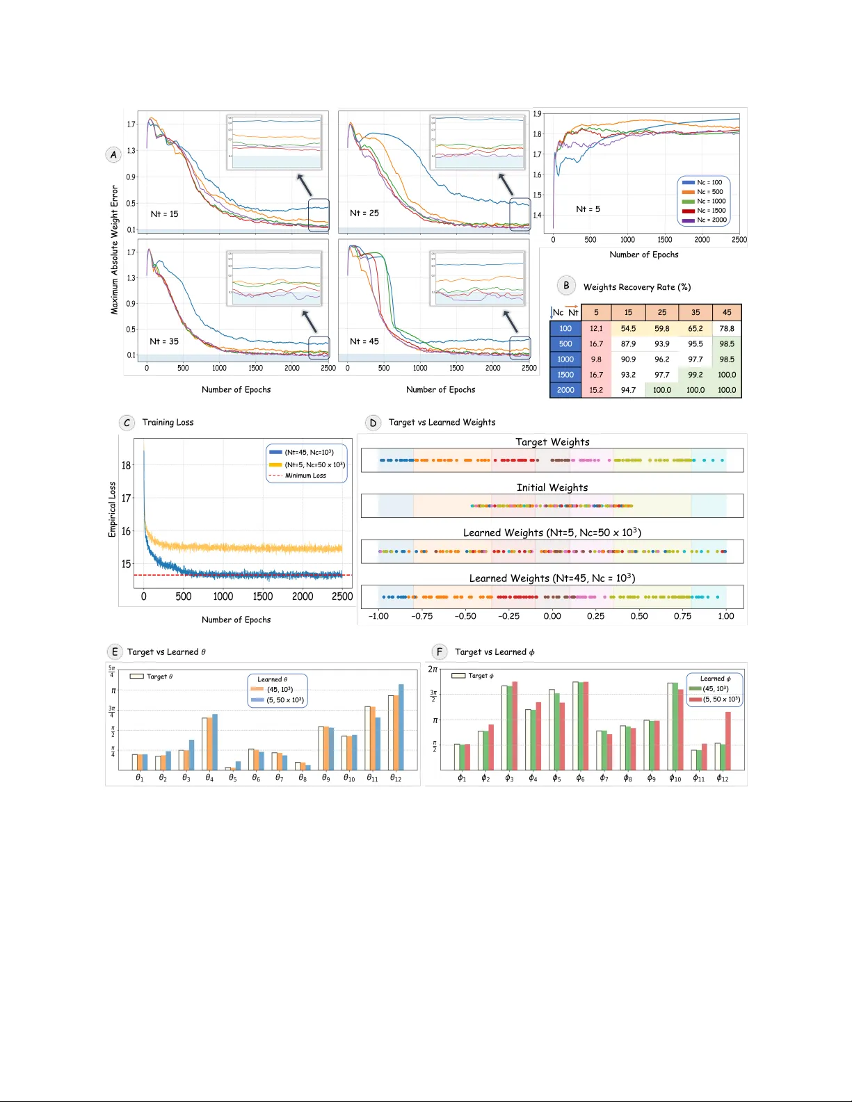
1 Quantum Hamiltonian Learning using T ime-Resolv ed Measurement Data and its Application to Gene Re gulatory Network Inference Mohammad Aamir Sohail ∗ , Ranga R. Sudharshan † , S. Sandeep Pradhan ∗ , Arvind Rao † ∗ Department of EECS, Uni versity of Michigan, Ann Arbor , USA † Department of Computational Medicine and Bioinformatics, Uni versity of Michigan, Ann Arbor , USA Abstract W e present a new Hamiltonian-learning framework based on time-resolved measurement data from a ﬁxed local IC-PO VM and its application to inferring gene regulatory networks. W e introduce the quantum Hamiltonian-based gene-expression model (QHGM), in which gene interactions are encoded as a parameter - ized Hamiltonian that governs gene expression evolution ov er pseudotime. W e derive ﬁnite-sample recovery guarantees and establish upper bounds on the number of time and measurement samples required for accurate parameter estimation with high probability , scaling polynomially with system size. T o recover the QHGM parameters, we develop a scalable v ariational learning algorithm based on empirical risk minimization. Our method reco vers netw ork structure efﬁciently on synthetic benchmarks and rev eals no vel, biologically plausible regulatory connections in Glioblastoma single-cell RNA sequencing data, highlighting its potential in cancer research. This framework opens new directions for applying quantum-like modeling to biological systems beyond the limits of classical inference. I . I N T RO D U C T I O N Quantum Hamiltonian learning (QHL) refers to the task of inferring the parameters of a Hamiltonian associated with a many-body quantum system without requiring resources that scale exponentially with the system size. This task is essential in areas such as quantum simulation, condensed matter physics, and the characterization of quantum de vices [1]–[6]. For example, in condensed matter physics, Hamiltonian learning allo ws the identiﬁcation of ef fecti ve spin-interaction models in quantum materials, based on spectroscopic measurements of spin excitations [6]. A conceptually straightforward approach to QHL is quantum process tomography [7]–[10]. Howe ver , this approach requires resources that scale exponentially with system size, making it impractical for real experiments. [11]. 2 T o overcome the prohibitive costs of process tomography , a wide range of efﬁcient QHL methods have been de veloped across div erse settings. For instance, sample-efﬁcient algorithms hav e been proposed for learning local Hamiltonians from Gibbs or thermal states [12]–[16], single eigenstates [17]–[20], and the steady state of the Hamiltonian [21], [22]. Additional methods focus on using measurements of local observables [23]–[25], short-time e v olution [26]–[29], and time-resolved measurements [30], [31]. Several works ha ve also proposed using a trusted quantum simulator to infer the Hamiltonian of an untrusted de vice [32]–[34]. Recent adv ances include scalable algorithms based on matrix product state (MPS), [35] and noise-resilient learning methods [29], [36]. Additionally , a series of works ha ve demonstrated Heisenberg-limited scaling for Hamiltonian learning [37]–[41]. In other words, the error in estimated parameters scales as the in verse of total ev olution time, rather than the square-root of total e volution time as seen in the standard quantum limit [42], [43]. QHL has been traditionally applied in quantum physics to understand particle interactions. Howe ver , this can be extended to understand the underlying interaction structure of complex systems, which may not be inherently quantum-scale but exhibit behavior that cannot be accurately described by classical probabilistic models. This broader viewpoint is central to the quantum-like modeling paradigm [44]–[46], which utilizes the mathematical tools of quantum information theory , such as non-commutativ e observables, superposition in Hilbert space, and quantum measurements modeled as positi ve operator v alued measure (PO VM), to model information processing in complex systems. As put forth in [47], the quantum formalism can be applied “not only to physical systems, but to systems of any origin — whether biological, social, or ﬁnancial — as long as their behavior exhibits some distinguishing features of quantum systems”. The quantum-lik e paradigm has been explored in div erse ﬁelds be yond physics, including cogniti v e science, decision theory , ﬁnance, and neuroscience [47]–[51]. An interesting application where quantum-like modeling can offer an advantage is the inference of gene regulatory networks (GRNs). The transcriptional state of a cell is highly dynamic and tightly regulated by complex interactions between genes, often mediated through multiple proteins. Understanding these regulatory relationships is critical for deciphering cellular behavior and function, yet represents one of the fundamental challenges in systems biology . In recent years, the increasing av ailability of large-scale single-cell RN A sequencing (scRNA-seq) data [52], which essentially captures the e xpression lev els of individual genes across cells, has greatly facilitated the de velopment and reﬁnement of computational tools for GRN inference. These datasets provide unprecedented resolution to capture cell-to-cell v ariability , enabling more accurate modeling of gene interactions across diverse cellular states and conditions. Current classical methodologies can be broadly classiﬁed into correlation-based [53] [54], tree-based ensemble methods [55] [56], information-theory- based [57], and Bayesian network-based models [58]. While these techniques have yielded valuable insights, they may fall short in capturing the nuanced and context-dependent nature of biological re gulation. Empirical 3 studies increasingly show that gene-expression data can violate the classical la w of total probability and present non-classical features such as interference of probabilities [49], [59]–[62], as well as violation of the Bell inequality in the macroscopic w orld [63]. Moreover , in cancer progression, certain cell types have been observed to exist in hybrid states, simultaneously expressing features of multiple phenotypes, in a manner reminiscent of quantum superposition [64], [65]. These observations suggest that the regulatory interactions in GRNs can be better modeled using a quantum-like paradigm. Recent research has started to explore quantum-like models for inferring complex biological networks [66]–[70]. A quantum circuit model has been proposed in [66] for GRN inference from scRNA-seq data, where each gene is represented as a qubit. Howe ver , the circuit construction is sensitiv e to gene ordering, as it prioritizes genes with higher activ ation ratios in the qubit mapping. The model also relies on the (classical) KL diver gence loss function [71], which requires ev aluating joint probability distributions, resulting in computational costs that scale exponentially with network size. Furthermore, existing methods lack a systematic framework for integrating multi-omics data, such as genomics, transcriptomics, and proteomics, thereby limiting their ef fectiv eness in practical biological applications. Building on these observ ations, we propose that the QHL framew ork of fers a powerful approach to modeling gene regulatory dynamics. It enables scalable and sample-efﬁc ient inference of complex, nonlinear interactions that classical methods might overlook. Additionally , it offers a ﬂexible foundation for integrating multi-omics data. Howe ver , applying QHL to GRNs is challenging from multiple perspecti ves. Existing QHL approaches are primarily tailored for quantum man y-body systems and rely on entangled initial states, random Pauli measurements, Gibbs states, or access to eigenstates, resources that do not have direct relev ance in the context of GRNs. T o address this gap, we formulate a new Hamiltonian learning problem grounded in statistical learning theory and motiv ated by the biology of GRNs. Belo w , we summarize the ke y contrib utions of this work. 1 . Hamiltonian Learning from Time-Resolv ed Measurement Data: W e formulate a new Hamiltonian learning problem using measurement outcomes from a ﬁxed local informationally complete PO VM (IC-PO VM) collected at multiple times, starting from a ﬁxed initial state. W e characterize the sample complexity in terms of the number of time samples, denoted as N t , and the number of measurement outcomes per time sample, denoted as N c , sufﬁcient to achiev e small estimation error with high probability (see Theorem 1). Both N t and N c scale polynomially with the number of qudits. Furthermore, we establish a ﬁnite-sample uniform con v ergence bound for the empirical loss (see Theorem 2). 2 . Quantum Hamiltonian-Based Generativ e Modeling of Gene Expression: W e instantiate our QHL framework in the context of GRNs and introduce the quantum Hamiltonian-based gene-expression model (QHGM) (see Fig. 1) for simulating GRNs. In this model, genes are treated as qubits. The QHGM generates gene-expression 4 data by modeling re gulatory interactions as quantum-like couplings encoded in a parameterized Hamiltonian. Each single-qubit IC-PO VM outcome corresponds to the expression le vel of an individual gene, and together they yield the gene-expression proﬁle of a cell. W e employ pseudotime [72], which orders cells along inferred de velopmental trajectories deriv ed from scRN A-seq data, as an approximate analogue of physical ev olution time. W e construct a Hamiltonian for GRN by deﬁning biologically interpretable interaction terms using tensor products of computational basis states. 3 . Scalable and Sample-Efﬁcient Network Inference Algorithm: W e dev elop a scalable v ariational quantum network inference algorithm (VQ-Net) for learning QHGM parameters from scRN A-seq data (see Methods and Fig. 2). VQ-Net is built on an empirical risk minimization framework and minimizes the negati v e log- likelihood loss o ver mini-batches of scRN A-seq data collected at multiple pseudotime bins. 4. Numerical Ev aluation on Synthetic Data: W e provide comprehensiv e numerical results and performance of VQNet on synthetic gene-expression data generated by QHGM (see Fig. 3). These experiments validate the theoretical sample-comple xity bounds deri ved in our learning frame work, demonstrating the trade-of f among the number of time samples, the number of measurement samples per time, and estimation accuracy . 5. Application to glioblastoma scRN A-seq data: W e apply our framework to scRN A-seq from glioblastoma (GBM) patients [73], focusing on the gene regulatory programs governing differentiation of OPC-like cells (see Fig. 4). GBM is the most common malignant primary brain tumor, with poor prognosis and complex cellular heterogeneity [74], [75]. T o our kno wledge, this is the ﬁrst application of quantum-like modeling to infer biologically relev ant re gulatory networks in cancer research. Our results re veal potential GRN structures and interaction patterns that reﬂect the cellular plasticity within malignant OPC-like populations, opening ne w av enues for quantum-dri ven e xploration of information ﬂo ws in biological systems. I I . M A I N R E S U L T S W e hav e organized our ﬁndings into three main subsections. The ﬁrst subsection presents our theoretical frame work for Hamiltonian learning. The second subsection builds on this foundation by demonstrating how the same frame work can be applied to infer GRNs. In the ﬁnal subsection, we present numerical results on synthetic and real scRN A-seq data. A. Hamiltonian Learning using T ime Dynamics of IC-PO VM Deﬁnition 1 (Statistical Model) . Consider a Hamiltonian H( w ) = P c j =1 w j H j that acts on a quantum system of n qudits, each of dimension d . It consists of c local terms { H j } acting on a subset of qudits and a parameter vector w ∈ W B := { w ∈ R c : ∥ w ∥ 2 ≤ B } . F or an evolution time t , deﬁne the corr esponding e volved quantum state as follows: ρ t ( w ) := U t ( w ) ρ 0 U † t ( w ) , wher e U t ( w ) = exp {− i t H( w ) } , and ρ 0 is the initial state. After the evolution, an IC-PO VM measurement, denoted as Λ := { Λ m : m ∈ M} , is performed on each qudit, 5 pr oducing an outcome in a ﬁnite set M . This r esults in a tensor ed-pr oduct measurement acting on the entir e system of dimension D = d n . This measur ement generates an outcome vector m := ( m (1) , · · · , m ( n ) ) ∈ M n at time t accor ding to the pr obability given as ϕ ( m | t, w ) := tr(Λ m ρ t ( w )) , wher e Λ m = (Λ m (1) ⊗ · · · ⊗ Λ m ( n ) ) . Consider a set of N t e volution times, denoted as T := { t 1 , t 2 , . . . , t N t } , independently drawn from a design distribution π ( t ) over (0 , t max ] . For each t i ∈ T , we are giv en N c measurement outcomes, denoted as { m ( i, 1) , · · · , m ( i, N c ) } . Here, m ( i,k ) is a n -length vector that denotes the k -th outcome collected at time t i . These outcomes are independently and identically generated according to the probability distribution ϕ ( m | t i , w ∗ ) determined by (unknown) parameters w ∗ ∈ W B , i.e., each measurement arises from an inde- pendent preparation of ρ 0 , follo wed by e v olution for time t i , and performing the IC-PO VM Λ . Note that the outcomes { m (1 ,k ) , m (2 ,k ) , · · · , m ( N t ,k ) } are independent but not identically distrb uted. Objective: Giv en the collection of measurement outcomes across all times, our goal is to obtain an estimate b w := b w  { m ( i,k ) } N t , N c i =1 ,k =1  ∈ W B of parameter w ∗ such that for any δ ∈ (0 , 1) , a bound of the following form holds with probability at least (1 − δ ) : ∥ b w − w ∗ ∥ 2 ≤ g ( δ, N c , N t ) . T o obtain an estimator b w that meets the high-probability error bound stated above, we consider the em- pirical risk minimization frame work. Giv en N t time samples and N c independent and identically distributed measurement outcomes for each time t , deﬁne the empirical and expected loss as follo ws b L ( w ) := 1 N t N t X i =1 1 N c N c X k =1 ℓ  ϕ ( m ( i,k ) | t i , w )  and L ( w ) := E t ∼ π  E m ∼ ϕ ( ·| t, w ∗ ) [ ℓ ( ϕ ( m | t, w ))]  , where ℓ ( · ) := − log ( · ) . Then, we obtain the minimizer of empirical loss b L ( w ) as b w := arg min w ∈W B b L ( w ) . Assumptions: W e state the following assumptions. A ( i ) The expected loss function L ( w ) is µ 0 - strongly con v ex (SC) over W B . A ( ii ) The likelihood function ϕ is bounded, ϕ ( m | t, w ) ≥ p min > 0 for all m ∈ M n , t ∈ (0 , t max ] , and w ∈ W B . Our main result is a sample-ef ﬁcient learning algorithm for the QHL problem. W e provide a detailed proof in the Method section. Theorem 1. F or the Hamiltonian learning pr oblem described above, ﬁx a conﬁdence δ > 0 and an empirical SC tolerance ε > 0 . Under the assumptions stated above, if the number of sampled times N t and the number of measur ement outcomes per time N c ar e c hosen such that 6 N t = ˜ O  c 3 ε 2 log  1 δ  and N c = ˜ O  c 3 ε 2 log  N t δ  , wher e ˜ O hides logarithmic factors in c and 1 /ε , as well as ﬁxed constants µ 0 , B , t max , and p min . Then, with a pr obability at least (1 − 2 δ ) , the empirical loss b L is (1 − 2 ε ) µ 0 -str ongly conve x over W B . Furthermor e, suppose b w ∈ in terior( W B ) with pr obability 1. Then, with pr obability at least (1 − 3 δ ) , the empirical minimizer satisﬁes ∥ b w − w ∗ ∥ 2 ≤ O  1 (1 − 2 ε ) µ 0 r c N c log  N t δ   . (1) Scaling with system size. The above bounds sho w that the required number of sampled times N t and the number of measurement results per time N c scale polynomially with the number of Hamiltonian parameters. When the number of parameters c scales polynomially in n , then both N t and N c also scale polynomially with the number of qudits. Insufﬁcient N t but N c is lar ge. Note that for a gi ven sampled time t i , it may happen that different parameter v alues can induce the same measurement distrib utions. In particular, for a giv en time t , there may e xist w  = w ∗ such that ϕ ( ·| t, w ) = ϕ ( ·| t, w ∗ ) . If the number of time samples N t is too small, such non-identiﬁability can persist across the entire set of sampled times, so that distinct parameters remain indistinguishable from the observed data. Increasing N c only reduces the variance in estimating the per-time e xpected loss. As a result, increasing N c alone cannot compensate for insuf ﬁcient identiﬁability caused by the limited time samples. Sufﬁciently larg e N t but N c = 1 . If the number of time samples N t becomes very large, taking only a single measurement at each time point is insuf ﬁcient for accurate parameter recov ery . When the number of measurements per time is small, the empirical estimate of the measurement distribution at each time is dominated by sampling noise. Consequently , although increasing N t provides suf ﬁcient identiﬁability of the parameters, the information av ailable at each time remains too noisy to be useful. W e next establish a ﬁnite-sample uniform con ver gence guarantee for the empirical loss b L around the expected loss L ov er W B . The following theorem shows that as the number of time samples N t and the number of measurements per time sample N c increase, b L uniformly concentrates around L , thus justifying the use of empirical risk minimization as a faithful approximation to the expected risk minimization problem. Theorem 2. Under the assumption A ( ii ) , for any δ > 0 , the following non-asymptotic uniform deviation bound holds with pr obability at least  1 − 4 δ ) : sup w ∈W B   b L ( w ) − L ( w )   ≤ 72 √ π cB L p √ N t + 2 p 2 log (2 D ) p min √ N c − 3 log p min  s 2 log (2 /δ ) N t + s log(2 N t /δ ) 2 N c  . (2) 7 An important implication of this uniform con ver gence result is that it provides a key ingredient for establishing asymptotic strong consistency of the empirical minimizer as N t , N c → ∞ (see [76, Theorem 4.10]). B. Application to Gene Re gulatory Network Infer ence Gene Regulatory Network gene - to - qubit mapping 𝜙(𝐦|𝑡 , 𝒘) Outcome distribution g i 𝑤 !" g 3 g 4 g 5 g n g 1 g 2 |𝜓 ! (𝒘) ⟩ |𝜓 " ⟩ 𝑒 #$%& 𝐰 Pseudotime Evolution entangled state |𝜓 ! (𝒘) ⟩ 3 1 2 1 0 1 0 0 0 3 0 1 2 3 1 2 1 3 1 Nc Nt 0 2 1 2 1 2 2 0 1 2 0 2 0 2 0 1 2 2 3 1 2 0 1 2 1 1 1 0 1 0 2 0 1 0 1 1 1 2 2 3 2 1 3 1 1 0 1 0 2 3 2 1 2 1 1 0 1 2 1 n H 𝐰 = $ 𝑤 !" & 1 2 I − Z ! ⊗ Y " ( ! , " ) Parameterized Hamiltonian IC - POVM measurement Λ ' (") Λ ' ($) Λ ' (%) Discretized gene - expression profile g 1 g 2 g n Separable Init ial State 𝒢 = Figure 1: Overvie w of the quantum Hamiltonian-based gene-expression model (QHGM). A gene regulatory network (GRN) is mapped to a parameterized Hamiltonian H( w ) , where the presence of gene g i induces the action of a P auli- Y operator on gene g j with regulatory weights w ij . The model begins from an initial separable state, representing independent gene states. As the system ev olves along pseudotime, correlations between genes are gradually introduced, resulting in an entangled quantum state. At each pseudotime point, this state is measured using a ﬁx ed single-qubit IC- PO VM, producing a probability distribution ϕ ( m | t, w ) over measurement outcomes. Collecting repeated measurements outcomes at each pseudotime point yields discretized gene-expression proﬁles, denoted as G , with dimension ( N t , N c , n ) that serve as the observable data for inference. Here, N t is the number of pseudotime bins, N c is the number of independently measured cells per bin, and n is the number of genes in the network. Building on our QHL frame work, we apply it to GRNs and obtain a statistical generati ve model for gene- expression data, which we call the quantum Hamiltonian-based gene-e xpression model (QHGM) (see Fig. 1). In QHGM, for simplicity of exposition, we represent each gene as a qubit. The computational basis states | 1 ⟩ and | 0 ⟩ correspond to the transcriptional state of the gene, indicating whether it is e xpressed or une xpressed in a cell, respectiv ely . The model consists of three main components: ( i ) a Hamiltonian that encodes the 8 regulatory structure of the GRN, ( ii ) initial state preparation and pseudotime state ev olution, and ( iii ) an IC-PO VM measurement, each described in detail below . 1. Hamiltonian for GRNs: The regulatory interactions between genes are encoded in a parameterized Hamil- tonian as H( w ) = X ( i,j ) ∈E w ij 1 2 (I − Z i ) ⊗ Y j , (3) where E := { ( i, j ) : i, j ∈ { 1 , 2 , · · · , n } , i  = j } and n is the number of genes in the network. The weights w ij capture both the strength and direction of regulatory inﬂuence, with each w ij quantifying the ef fect of gene g i on gene g j . A positi ve w ij indicates acti v ation, meaning that the presence of gene g i promotes the e xpression of g j , whereas a negati ve w ij implies that g i suppresses g j . Each coef ﬁcient is bounded, i.e., | w ij | ≤ w max , to maintain biologically meaningful interaction strengths [77]–[79]. The magnitude | w ij | reﬂects the strength of regulation, with lar ger absolute values corresponding to stronger acti vating or repressing effects. W e exclude the self-interaction links, as the y correspond to intrinsic gene dynamics rather than inter-gene regulation. W e provide additional details on the construction of the GRN Hamiltonian in the Methods section. 2. Initial State Pr eparation and Pseudotime Evolution: The QHGM be gins by initializing the system in a separable state | ψ 0 ⟩ := n O i =1 | ψ ( i ) 0 ⟩ , where | ψ ( i ) 0 ⟩ = cos θ i | 0 ⟩ + e iϕ i sin θ i | 1 ⟩ . (4) Each qubit-state | ψ ( i ) 0 ⟩ represents the transcriptional state of g i as a point on the Bloch sphere, where sin 2 θ i and cos 2 θ i denote the prior probabilities of g i being expressed or unexpressed, respectively . The angle ϕ i encode its initial directional or kinetic phase information [80]. This initialization reﬂects an assumption that genes exist independently without correlations, with correlations emerging dynamically through the regulatory interactions encoded in the Hamiltonian. The system then ev olves following the Schr ¨ odinger equation d | ψ t ⟩ / d t = − iH( w ) | ψ t ⟩ , with the time-independent Hamiltonian H( w ) , yielding a ﬁnal state | ψ t ( w ) ⟩ = exp {− i t H( w ) } | ψ 0 ⟩ , where t represents the pseudotime, which corresponds to the temporal progression of cell-state transition. Pseudotime is the approximate position of cells along a trajectory that quantiﬁes the relati ve progression of the underlying biological process [81]. 3. Measur ement and Gene Expr ession Readout: Follo wing pseudotime ev olution, each qubit (gene) is measured using a single-qubit IC-PO VM { Λ m } 3 m =0 gi ven as Λ 0 = 1 4  I + 1 2 X + √ 3 2 Z  , Λ 1 = 1 4  I − 1 2 X − 1 √ 2 Y + 1 2 Z  , Λ 2 = 1 4  I − 1 2 X + 1 √ 2 Y − 1 2 Z  , Λ 3 = 1 4  I + 1 2 X − √ 3 2 Z  . (5) W e provide further details on the construction of IC-PO VM for GRN in Methods. The outcomes of the IC- PO VM measurement provide a discretized representation of the gene expression at a gi ven pseudotime. For 9 example, the measurement label for the j -th qubit, denoted by m ( j ) ∈ { 0 , 1 , 2 , 3 } , represents a discretized expression le vel of gene g j : m ( i ) = 0 indicates that gene g j is not expressed, while m ( j ) = 3 signiﬁes that gene g j is highly expressed in a cell. The overall measurement outcome vector is denoted as m = ( m (1) , m (2) , . . . , m ( n ) ) and spans 4 n possible joint outcomes. The probability distribution over these joint outcomes at pseudotime t is gi ven by ϕ ( m | t, w ) = ⟨ ψ t ( w ) | Λ m | ψ t ( w ) ⟩ . Collecting repeated measurement outcomes at each pseudotime t i ∈ { t 1 , · · · , t N t } yields a discretized gene-expression dataset G := { m ( i,k ) } N t , N c i =1 ,k =1 ∈ { 0 , 1 , 2 , 3 } N t × N c × n , which serv es as the observable data for inference. Here, N t denotes the number of pseudotime bins (discrete time points), N c denotes the number of independently measured cells (measurement outcomes) per bin, and n is the number of genes (qubits) in the network. This concludes the description of QHGM. Learning r e gulatory coefﬁcients w : Building on QHL using empirical risk minimization, we design a v ari- ational quantum network inference algorithm (VQ-Net) to learn the weights from the discretized scRN A- seq data collected at multiple pseudotime points. In this algorithm, the normalized scRNA-seq data is ﬁrst con v erted into four discrete v alues. During each iteration, the algorithm minimizes the av erage ne gati ve log- likelihood function across all pseudotime bins. Furthermore, if the priors θ i and ϕ i are not av ailable for the initial state preparation, the algorithm jointly learns these parameters alongside w . Further implementation details are provided in the Methods and summarized in Fig. 2. C. Numerical Experiments and Results W e e valuate the proposed VQ-Net through numerical e xperiments on synthetic data generated using QHGM. Moreov er , we demonstrate the usage of QHGM on the GBMap scRNA-seq data to infer GRNs with both kno wn and nov el regulatory interactions. Synthetic Data : T o ev aluate the performance of VQ-Net, we generate synthetic time-resolved measurement data using the QHGM as the ground-truth generati ve model. W e consider a 12 -qubit system with 132 randomly chosen weights w ij ∈ [ − 1 , 1] . A detailed description of the simulation setup, including data generation and training, is pro vided in Methods. Fig. 3 summarizes the empirical tradeof f between the number of times samples N t and the number of measurement per time sample N c . In Fig. 3A, we test different N t ∈ { 5 , 15 , 25 , 35 , 45 } and N c ∈ { 100 , 500 , 1000 , 1500 , 2000 } and report the maximum absolute weight error between learned weights and true weights ( max ( i,j ) | w ij − w true ij | ∈ [0 , 2] ) against training epochs. For N t = 5 , the error diver ges and ev entually saturates near the maximum error of 2 for all values of N c . This suggests potential issues with insufﬁcient empirical identiﬁability due to fewer time samples. In contrast, when N t exceeds 15, the error decreases monotonically and con ver ges towards 10 𝐦 !,# ! ! " #$ %&&# ! " " #$ '( ! # " #$ #)'# ! $ " #$ *( m = 0 m = 1 m = 2 m = 3 #$ +,-( #$ -(+( #$( # - Discretization of Normalized s cRNA - seq data Measurement 𝜙 Classical Optimizer Repeat until convergence Update (𝜽, 𝝓, 𝒘) 𝒘 (𝜽, 𝝓) Normalization + Pseudotime analysis cells genes g 1 g 2 g n |𝜓 ! (𝒘) ⟩ |𝜓 " ⟩ 𝑒 !"# . $ 𝐰 Λ 𝐦 /0123 4 Λ 𝐦 (𝒊,𝒌) & Λ 𝐦 (𝒊,𝒌) ' Initial State Preparation Normalized scRNA - seq data with Pseudotimes Pseudotimes t 1 t 2 t Nt genes cells Pseudotime Evolution g 1 g 2 g n g 1 g 2 g n Target Source Learned 𝒘 " Inferred GRN Learned weig hts A B C D E F t 1 ------- t Nt t 2 g 3 g 4 g 5 g 6 g 1 g 2 3 1 2 1 0 1 0 0 0 3 0 1 2 3 1 2 B 1 3 1 Nc Nt 0 2 1 2 1 2 2 0 1 2 0 2 0 2 0 1 2 2 3 1 2 0 1 2 1 1 1 0 1 0 2 0 1 0 1 1 1 2 2 3 2 1 3 1 1 0 1 0 2 3 2 1 2 1 1 0 1 2 1 n 𝒢 = 𝐿 + " 𝒘 = 1 BN # / (%,' ) − log (𝜙(𝐦 %,' |𝑡 % , 𝒘)) Gene Expression scRNA - seq data Figure 2: VQ-Net. (A) Raw scRN A-seq data are preprocessed, normalized, and assigned pseudotime values, providing a temporal ordering of cells along a de velopmental trajectory . (B) The normalized pseudotime-ordered scRNA-seq data are con verted into four discrete values, denoted as G , where N t denotes the number of pseudotime bins, N c denotes the number of independently measured cells per bin, and n is the number of genes in the network. (C) Prepares a separable initial state and ev olv es under the parameterized Hamiltonian H( w ) = P ( i,j ) w ij 1 2  I − Z i  ⊗ Y j , which encodes directed regulatory interactions. (D) For each pseudotime bin t i , the single-qubit IC-PO VM is applied as measurement observables on entangled e volv ed states conditioned on the discretized scRN A-seq data m ( i,k ) as input. Here, k is the index of the cell in the corresponding pseudotime bin. (E) The parameters ( θ , ϕ , w ) are optimized by minimizing the mini-batch empirical loss using a classical optimizer . (F) The learned weights w are visualized as a signed, asymmetric weight matrix, from which the GRN is inferred. 11 Figure 3: Performance of VQ-Net on the synthetic data generated using QHGM. (A) Maximum absolute weight error versus epochs for different numbers of sampled times N t and measurements per time N c . (B) Percentage of recov ered weights within 10% error , illustrating the tradeoff between empirical identiﬁability (controlled by N t ) and sampling variance (controlled by N c ). (C) Batch empirical loss during training is computed using a mini-batch of size 20 and 200 for N t = 45 and 5 , respecti vely . The results indicate con ver gence to the theoretical optimum for N t = 45 . (D) Learned weights compared to ground truth, demonstrating strong recovery for N t = 45 and dispersion for N t = 5 . (E–F) Recovered initial-state parameters ( θ , ϕ ) with relativ e errors of (0 . 0098 , 0 . 0194) for ( N t , N c ) = (45 , 10 3 ) and (0 . 1638 , 0 . 180) for ( N t , N c ) = (5 , 50 × 10 3 ) , respectiv ely . 12 zero. Additionally , more stable conv er gence and reduced error are observed as N c increases. In Fig. 3B, we report the percentage of recovered weights within a tolerance of 0 . 1 (i.e., less than 10% maximum absolute error). For all N t greater than 5 , the reco very rate improves monotonically as N c increases. Howe v er , when the number of measurements per time is small ( N c = 100 ), we observe a sharp de gradation in performance, up to a 30% drop in reco v ery rate (highlighted in yello w), relativ e to N c > 100 . The sudden decrease can be attributed to high sample v ariance at low N c , which results in noisy empirical estimates of the true likelihood function, ev en when there are enough time samples. In this scenario, the optimizer is signiﬁcantly inﬂuenced by sampling noise rather than structural information, causing many weights to exceed the 0.1 tolerance le vel. For N t = 5 , the recov ery rate decreases signiﬁcantly , by as much as 80% compared to larger values of N t (highlighted in red). This decline is likely due to parameter indistinguishability when the number of sampled time points is small. Speciﬁcally , multiple distinct weight conﬁgurations produce nearly identical measurement statistics across the observed times, resulting in a drop in weight recov ery accuracy that does not reliably improv e even with increasing N c . For e xample, the relativ e error , deﬁned as ∥ w learned − w true ∥ / w true , for ( N t , N c ) = (5 , 50 × 10 3 ) is 1.0055, whereas it is 1.251 for ( N t , N c ) = (5 , 10 2 ) . Fig. 3C shows the batch empirical loss, computed as the a verage negati ve log-likelihood o ver a mini-batch, versus training epochs. In this ﬁgure, ( N t , N c ) = (45 , 10 3 ) (blue) con verges to the theoretical minimum (dashed line), which corresponds to the expected negati ve log-likelihood loss averaged ov er the sampled times. In contrast, ( N t , N c ) = (5 , 50 × 10 3 ) (yello w) remains trapped above the optimum. The learned weights (color- coded by target bins) corresponding to these two cases are sho wn in Fig. 3D. For N t = 45 , the learned weights cluster tightly around their true v alues. For N t = 5 , the learned weights remain dispersed despite recei ving the same initialization. Finally , in Fig. 3E and F , we inspect the reconstructed initial-state parameters ( θ , ϕ ) . F or (45 , 10 3 ) , the relati v e errors for θ and ϕ are 0 . 0098 and 0 . 0194 , respectiv ely . Interestingly , ev en when the weights are not accurately estimated at (5 , 50 × 10 3 ) , the initial-state parameters are learned with a lower error of 0 . 1638 for θ and 0 . 180 for ϕ . This indicates that VQ-Net can simultaneously infer both the weights and the initial state, and the estimation of initial-state parameters is comparati vely more robust to changes in N t and N c than the recov ery of weights. These observ ations align closely with our theoretical analysis: the indistinguishability of the parameters is gov erned by the number of times sampled N t , while the sampling v ariance of the empirical loss is controlled by the number of measurements per time N c . Therefore, simply increasing N t or N c on its o wn is not enough to driv e the weight estimation error to zero. T o achie v e consistent reco very , it is necessary to ha ve both a sufﬁcient number of time samples and a suf ﬁcient number of measurements at each time point. GBMap scRNA-seq data : W e implemented the VQ-Net to build QHGM using the core GBmap scRN A- seq data comprising 16 independent studies and 109 patients, post standardization and batch normalization 13 [73]. W e focused on Differentiated-lik e and Stem-like cells in the annotation lev el 2 classiﬁcation, yielding approximately 127,000 cells in total. At annotation lev el 3, these cells were further classiﬁed as Astrocyte-like (A C-like) (50,847), Mesench ymal-like (MES-like) (33,167), Neural Progenitor Cell-like (NPC-like) (22,117), and Oligodendrocyte Progenitor Cell-like (OPC-lik e) (21,390). Pseudotime is inferred using the VIA algorithm [72], with an OPC-like cell as the root representing the putati ve progenitor state and A C-like and MES-lik e cells as terminal endpoints (see Fig. 4A). Cells are embedded in UMAP space based on the 5,000 most v ariable genes, and a streamplot is overlaid on the embedding to visualize the dominant probabilistic ﬂo w along pseudotime. Higher pseudotime values correspond to more dif ferentiated states, and the trajectory highlights branching points and intermediate transitional states along the dif ferentiation continuum. T o examine the gene regulatory dynamics along this trajectory , we considered a set of 14 genes: BCAN , STMN1 , HES6 , ETV1 , CADM2 , MMP16 , CKB , LIMA1 , VCAN , JPT1 , ASCL1 , CDK4 , TUBB2B , and NCAM1 . A detailed description of the data preparation and training details is pro vided in Methods. The learned weights are shown in Fig. 4B, which illustrates the median learned weights across independent training instances. T o quantify interaction selecti vity , we computed the coefﬁcient of variation (CV), deﬁned as the ratio of the standard de viation to the absolute v alue of the mean, separately for positive and neg ativ e learned weights (Fig. 4C). A high CV indicates selectiv e regulation, in which a gene strongly inﬂuences only a subset of the gene set, whereas a low CV reﬂects broad and more uniform re gulatory inﬂuence across the gene set. Fig. 4D shows the inferred GRN, consisting of the strongest regulatory interactions, deﬁned by row-wise selection of the top 15th percentile of positi ve and ne gati ve weights. T o validate the accuracy of these inferred interactions, we compared the weights learned via VQ-Net against kno wn regulatory pairs reported in the literature. As seen in Fig. 4D, QHGM correctly identiﬁes ASCL1’ s broad regulatory inﬂuence and recovers strong interactions with targets such as BCAN , CDK4 , and CKB , conﬁrming its established role in dri ving GBM heterogeneity [82]. Nodes like STMN1 , inte grate various regulatory inputs that have opposing effects. This is consistent with the known sensitivity of microtubule dynamics and cell cycle regulators to competing upstream signals [83]. The cyclin-dependent kinase axis, particularly CDK4 / 6 , is well-established as a driver of GBM cell proliferation and cell-cycle progression, with inhibition altering subtype programs in proneural stem-like cells supporting dynamic reprogramming under perturbation [84] [85]. Proliferation-associated genes ( CDK4 , STMN1 , TUBB2B ) are coupled to extracellular matrix (ECM) and cell-adhesion components ( BCAN , VCAN , NCAM1 , MMP16 ). This aligns with the literature on ECM proteoglycans (e.g., versican/ VCAN ), which promotes glioma proliferation and in v asion [86], and adhesion molecules that mediate GBM cell migration in a context-dependent manner [87]. Beyond the central hub structure, the model captures speciﬁc pairwise regulatory dynamics that are well supported by functional biology studies. Also, QHGM recovers biologically meaningful feedback regulatory 14 A C Cell type composition Inferred GRN D Gene Regulatory Pattern Classification B Learned Weights Cell Types – Level 2 Differentiated - like Stem - like Cell Types – Level 3 AC - like MES - like N PC - like OPC - like Pseudotime values 0.0 0.2 0.4 0.6 0.8 1.0 X Y Pseudotime streamplot AC - like MES - like N PC - like OPC - like Figure 4: Inferred GRN from QHGM on GBMap scRNA-seq data. (A) Cells are shown at increasing annotation granularity (Lev el 2 and Lev el 3) at UMAP coordinates. The trajectory inference is set with an OPC-like cell as the root node and progresses to ward AC-lik e and MES-like cell types speciﬁed as terminal endpoints. The streamplot overlaid on the UMAP embedding visualizes this progression, showing the dominant probabilistic ﬂow of cells along pseudotime, where higher pseudotime v alues correspond to more dif ferentiated states. (B) Heatmap of median learned weights across 10 simulations, which summarizes central tendencies across simulations. (C) Gene-wise classiﬁcation of regulatory behavior based on the coef ﬁcient of variation (CV) of positi ve and negati v e weights across simulations. The joint CV analysis distinguishes genes with selectiv e, stable acti vation or repression from those e xhibiting high v ariability , providing a quantitative measure of re gulatory consistency and context dependence. (D) GRN is inferred from the learned weights by selecting the top 15th percentile of positive (activ ation) and negati ve (repression) Hamiltonian weights separately , visualized as a directed network. Green and blue edges denote acti v ating and repressing interactions, respectiv ely . 15 loops. Notably , the model identiﬁes a positiv e association between VCAN and BCAN . This ﬁnding aligns with analyses comparing high versus low VCAN expression groups, where increased VCAN le v els were accompanied by upregulation of BCAN [86]. These results suggest that our quantum-lik e model demonstrates high precision in recov ering interactions. Overall, QHGM re veals extensi ve feedback loops and context-dependent sign switching, particularly in- volving lineage regulators such as ASCL1 , which has been implicated in multiple biological contexts, such as proneural transcriptional programs [88] and the neural stem cell-like features of glioma stem cells [89]. Such context dependency indicates that regulatory ef fects are not ﬁxed, instead v ary with the global state of the cell, consistent with the heterogeneity observed in GBM stem-like populations and dynamic state transitions [90]. Moreov er , the order and combination of regulatory events, such as lineage speciﬁcation versus microen vironmental engagement, can yield distinct downstream outcomes, supporting the notion that OPC-like GBM cells occupy a continuum of regulatory states rather than discrete phenotypes. The inferred GRN re v eals that OPC-lik e GBM states are gov erned by a densely interconnected regulatory architecture rather than by linear or modular signaling pathways. Collectiv ely , these results suggest that regulatory information in OPC-like cells propagates through interfering, conte xt-dependent, and non-separable pathways, producing dynamic cellular states that are not adequately captured by classical additive or modular gene regulatory models. I I I . D I S C U S S I O N In this work, we introduce a framework for Hamiltonian learning based on time-resolved measurement outcomes from a ﬁxed local IC-PO VM, and the system ev olves from a ﬁxed initial state. W e e valuate the QHL problem from a non-asymptotic perspective, deriving sample comple xity bounds that scale polynomially with the number of qudits. Our approach ﬁrst establishes the strong con ve xity of the empirical loss with high probability , which allows for a rigorous error bound between the empirical minimizer and the true parameters w ∗ . Furthermore, using Rademacher complexity arguments, we obtain a high-probability , ﬁnite- sample uniform conv er gence guarantee for the empirical loss. The resulting bound identiﬁes the contrib utions of two distinct stochastic sources: a N − 1 / 2 t term arising from the time sampling and a N − 1 / 2 c term arising from the ﬁnite number of measurement outcomes collected at each time point. Although these terms provide a baseline for con v ergence, tighter error bounds can be found by exploiting the local structure of the loss. For example, through local Rademacher complexity [91], one can potentially achie v e faster rates of order O (1 / N t  and O (1 / N c  . A promising direction is de veloping a learning algorithm that achiev es Heisenberg-scaling error bounds in the ﬁxed-measurement-model setting. Another natural next step is to move beyond closed- system dynamics and in v estigate open-system e volution, where learning non-unitary generators introduces ne w questions around identiﬁability and sample complexity . 16 Having established the theoretical guarantees of QHL, we next apply it to GRN inference. In contrast to quantum circuit-based approaches [66], our Hamiltonian formulation is agnostic to gene ordering, and the computational comple xity of VQ-Net scales polynomially with the number of genes, making it suitable for large GRNs. From a modeling perspecti ve, the QHGM provides a quantum-like representation of biological regulation: regulatory interactions correspond to coupling terms in the Hamiltonian and pseudotime play the role of a physical ev olution time. This viewpoint may offer deeper insight into biological netw orks that exhibit non-classical statistical features such as interference and contextuality [59], [60], which are challenging to capture with classical graphical models. A practical advantage of the Hamiltonian formulation is extensibility and expressi vity . The QHL frame work can incorporate multi-omics data (gene expression [92], chromatin accessibility [93], transcription factor binding [94], epigenetics [95], etc.) by adding corresponding terms to the Hamiltonian or introducing multiple measurements. Higher-order re gulatory interactions can be represented via hypergraph-inspired Hamiltonians (e.g., k -local terms for k > 2 ), enabling models that go beyond pairwise interactions [96]. Further , av enues to incorporate additional ancillas corresponding to external factors (other genes, en vironmental factors), such as open system characterizations, may also be worth looking at. All of these directions provide a structured conceptual path toward integrating multi-scale biological mechanisms and exogenous terms within a uniﬁed inference frame work. Beyond genomics, this Hamiltonian perspectiv e suggests potential applications in other network ed systems. A compelling direction is modeling mind–body interactions using time-series data from IoT wearables (e.g., heart-rate v ariability , stress markers, behavioral signals), as well as in e volving social systems. Such data exhibit contextuality and interference-like effects that violate classical Markov assumptions, suggesting that quantum-like models may re v eal underlying information structures in human physiology and social beha vior , analogous to quantum-like dependencies in GRNs. Finally , although we demonstrate the usage of the QHL frame work on GRN inference, the methodology is not speciﬁc to genomics. This can be extended to quantum many-body learning problems, and other quantum-like systems, such as social and economic networks, where contextual or non-classical probabilistic ef fects may arise. I V . M E T H O D S In this section, we present the proof of Theorems 1 and 2 and outline the technical details of QHGM, VQ- Net, and the training details of our numerical results. W e begin by introducing the necessary preliminaries used in the proofs. W e then describe the construction of the parameterized Hamiltonian used to model GRNS (Eq. (3)), follo wed by the construction of the IC-PO VM measurements employed in our frame work (see Eq. (5)). Next, we will provide the details of the VQ-Net algorithm. Finally , we will outline the data generation and training details used in our numerical results. 17 A. Pr eliminaries Let H := C D denote the D -dimensional Hilbert space, which serves as the conﬁguration space for quantum states. For the rest of the paper , ∥ · ∥ denotes the Euclidean norm for vectors and the spectral (or Schatten- ∞ ) norm for matrices unless otherwise stated. W e use ∥ · ∥ p to denote Schatten p -norm for matrices for p ∈ [1 , ∞ ) . Deﬁnition 2 (IC-PO VM [97]) . An IC-PO VM Λ := { Λ m } m ∈M is a ﬁnite collection of positive semideﬁnite operator s that sum to the identity , and span the space of Hermitian operators Herm( H ) , i.e, Λ m ≥ 0 , X m ∈M Λ m = I , and span { Λ m } m ∈M = Herm( H ) . The minimum number of elements required for informational completeness is M min = D 2 . Lemma 1 (Matrix Bernstein-type inequality [98, Corollary 6.2.1]) . Let µ X be a ﬁxed d 1 × d 2 matrix. Construct a random matrix X ∈ C d 1 × d 2 such that E X = µ X and ∥ X ∥ ≤ L. Let ¯ X n := 1 n n X k =1 X k , wher e { R k } n k =1 ar e independent copies of R . Then, for all t ≥ 0 , Pr  ∥ ¯ X n − µ X ∥ ≥ t  ≤ ( d 1 + d 2 ) exp  − nt 2 / 2 σ 2 + 2 Lt/ 3  , (6) wher e σ 2 is the per-sample second moment, deﬁned as σ 2 := max    E (XX † )   ,   E (X † X)    . In other wor ds, for any δ ∈ (0 , 1) , the following inequality holds: ∥ ¯ X n − µ X ∥ ≤ s 2 σ 2 n log  ( d 1 + d 2 ) δ  + 2 L 3 n log  ( d 1 + d 2 ) δ  . (7) with pr obability at least (1 − δ ) . Lemma 2. Consider a ﬁnite sequence { Λ k } of ﬁxed D × D Hermitian matrices, and let { σ i } be i.i.d. Rademacher r andom variables. Then the following inequality holds: E σ    X k σ k Λ k    ≤ p 2 log (2 D )    X k Λ 2 k    1 / 2 . Pr oof. The proof is provided in Appendix C. Lemma 3. Consider a time-independent Hamiltonian H( w ) = P c k =1 w k H k . Let U t ( w ) = e − it H( w ) and assume the system starts in the state ρ 0 . F or an observable Λ m satisfying ∥ Λ m ∥ ≤ 1 , deﬁne ϕ ( m | t, w ) := tr(Λ m ρ t ( w )) . Then, for every m ∈ M n and t ∈ (0 , t max ] , the following statements hold. ( i ) The likelihood function ϕ ( m | t, w ) is twice differ entiable in W B . The ﬁrst-or der partial derivative with r espect to the par ameter w k is given by ∂ ∂ w k tr(Λ m ρ t ( w )) = − i Z t 0 tr  Λ m ( t )  H k ( s ) , ρ 0   d s. (8) 18 Mor eover , the second-or der partial derivative with r espect to parameter s w j and w k is given by ∂ 2 ∂ w j ∂ w k tr(Λ m ρ t ( w )) = − Z t 0 Z s 1 0 tr  Λ m ( t )  H j ( s 1 ) , [H k ( s 2 ) , ρ 0 ]   d s 2 d s 1 − Z t 0 Z s 1 0 tr  Λ m ( t )  H k ( s 1 ) , [H j ( s 2 ) , ρ 0 ]   d s 2 d s 1 , (9) wher e Λ m ( t ) := U † t ( w ) Λ m U t ( w ) , and H k ( s ) := U † s ( w ) H k U s ( w ) . ( ii ) Bounded gradient and hessian. – F or all w ∈ W B , ∥∇ w ϕ ( m | t, w ) ∥ ≤ L ϕ and ∥∇ 2 w ϕ ( m | t, w ) ∥ ≤ L 2 ϕ . ( iii ) Lipschitz continuity . F or all w , w ′ ∈ W B , – | ϕ ( m | t, w ) − ϕ ( m | t, w ′ ) | ≤ L ϕ ∥ w − w ′ ∥ – ∥∇ w ϕ ( m | t, w ) − ∇ w ϕ ( m | t, w ′ ) ∥ ≤ L 2 ϕ ∥ w − w ′ ∥ – ∥∇ 2 w ϕ ( m | t, w ) − ∇ 2 w ϕ ( m | t, w ′ ) ∥ ≤ 2 L 3 ϕ ∥ w − w ′ ∥ , wher e L ϕ := 2 t max √ c ∥ H ∥ ∞ , max . Pr oof. The proof is provided in Appendix D. B. Pr oof of Theorem 1 Pr oof Outline : The proof establishes a ﬁnite-sample error bound between ˆ w and w ∗ by ﬁrst sho wing that the empirical loss inherits the strong con ve xity of the expected loss with high probability . The proof begins by observing that the complete set of measurement outcomes { m ( i,k ) } N t , N c i =1 ,k =1 is jointly independent but not identically distributed. Howe ver , for each time index i , outcomes are independent and identically distrib uted. This structure motiv ates decomposing the difference between the empirical and expected Hessian into two terms, ﬁrst measuring deviation within the conditional samples { m ( i,k ) } N c k =1 for each time index i , and the second term measuring deviation across the time. By applying the matrix Bernstein inequality (Lemma 1) to both terms in this decomposition, we show that the empirical Hessian concentrates near its expectation pointwise for each w ∈ W B with high probability . W e then employ a cov ering argument [76, Chapter 5] to extend this concentration uniformly o ver W B . By applying W eyl’ s inequality [76, Equation 8.9] and in v oking assumption A(i) , we establish the empirical strong con ve xity of the loss, ensuring a unique empirical minimizer ˆ w with high probability . Howe ver , ev en b L has a unique minimizer , ˆ w can still be distant from w ∗ . Therefore, under the high-probability e vent of empirical strong conv exity , we bound the distance ∥ ˆ w − w ∗ ∥ 2 by the norm of the gradient of the empirical loss at the true parameter , ∥∇ ˆ L ( w ∗ ) ∥ . Using Lemma 1 again, we bound this gradient norm, which in turn provides a ﬁnite-sample bound that v anishes as N t , N c → ∞ , ensuring that the unique empirical minimizer concentrates around w ∗ . 19 Let b H ( w ) := ∇ 2 b L ( w ) denote the Hessian of the empirical loss. W e begin the proof by introducing the fol- lo wing deﬁnitions: b H ( i,k ) ( w ) := −∇ 2 w log( ϕ ( m ( i,k ) | t i , w )) and ¯ H t i ( w ) := E ϕ ( ·| t i , w ∗ ) [ −∇ 2 w log( ϕ ( m | t i , w ))] . Next, consider the follo wing inequalities: ∥ b H ( w ) − ¯ H ( w ) ∥ ≤    b H ( w ) − 1 N t N t X i =1 ¯ H t i ( w )    +    1 N t N t X i =1 ¯ H t i ( w ) − ¯ H ( w )    ≤ 1 N t N t X i =1    1 N c N c X k =1 b H ( i,k ) ( w ) − ¯ H t i ( w )    +    1 N t N t X i =1 ¯ H t i ( w ) − ¯ H ( w )    ≤ T 1 + T 2 , where T 1 := max i ∥ 1 N c P N c k =1 b H ( i,k ) ( w ) − ¯ H t i ( w ) ∥ and T 2 := ∥ 1 N t P N t i =1 ¯ H t i ( w ) − ¯ H ( w ) ∥ . Note by using Jensen’ s inequality and Lemma 3, we establish a bound on ∥ b H ( i,k ) ( w ) ∥ and ∥ ¯ H t i ( w ) ∥ for a giv en time t i . For e v ery m ∈ M n , w ∈ W B , and t ∈ (0 , t max ] , we hav e ∥ − ∇ 2 w log( ϕ ( m | t, w )) ∥ ≤ 2( L ϕ /p min ) 2 and ∥ ¯ H t ( w ) ∥ ≤ 2( L ϕ /p min ) 2 , (10) where L ϕ = 2 t max √ c ∥ H ∥ ∞ , max . The proof is provided in Appendix E. Next, we bound the terms T 1 and T 2 using the follo wing proposition. Proposition 1. F or each w ∈ W B , and for all ε 1 , ε 2 ≥ 0 , the following inequality holds: (W ithin-time concentration.) Pr { T 1 ≥ ε 1 } ≤ 2 c N t exp  − N c ε 2 1 / 2 σ 2 + 4 ε 1 ( L ϕ /p min ) 2 / 3  , (11) (Acr oss-time concentration.) Pr { T 2 ≥ ε 2 } ≤ 2 c exp  − N t ε 2 2 / 2 σ 2 + 4 ε 2 ( L ϕ /p min ) 2 / 3  , (12) wher e σ 2 := 4( L ϕ /p min ) 4 . The proof can be found in Appendix F. Finally , combining the bounds on T 1 (11) and T 2 (12), and letting ε 1 = ε 2 = εµ 0 / 2 , we conclude that for each w ∈ W B , and for all ε > 0 , Pr {∥ b H ( w ) − ¯ H ( w ) ∥ ≥ εµ 0 } ≤ Pr { T 1 ≥ εµ 0 / 2 } + Pr { T 2 ≥ εµ 0 / 2 } ≤ 2 c  N t exp  − N c µ 2 0 ε 2 / 8 σ 2 + 2 εµ 0 ( L ϕ /p min ) 2 / 3  + exp  − N t µ 2 0 ε 2 / 8 σ 2 + 2 εµ 0 ( L ϕ /p min ) 2 / 3  . (13) W e now extend the pointwise bound to hold uniformly ov er W B . T o this end, we ﬁrst establish the Lipschitz continuity of b H and ¯ H . The proof is provided in Appendix G. Proposition 2. F or every m ∈ M n and t ∈ (0 , t max ] , both the expected Hessian and the empirical Hessian ar e Lipsc hitz continuous. ∥ b H ( w ) − b H ( w ′ ) ∥ ≤ 7( L ϕ /p min ) 3 ∥ w − w ′ ∥ and ∥ ¯ H ( w ) − ¯ H ( w ′ ) ∥ ≤ 7( L ϕ /p min ) 3 ∥ w − w ′ ∥ , for each w , w ′ ∈ W B . 20 Fix η > 0 , to be speciﬁed later . T o control the supremum o ver W B , we co ver W B with an η -net. That is, there exists a ﬁnite set N η ⊂ W B such that for ev ery w ∈ W B , there exists w ′ ∈ N η with ∥ w − w ′ ∥ 2 ≤ η . The cardinality of such a net can be bounded as N η := |N η | ≤ ( 3 B η ) c , where the inequality follows from the standard bound on the co vering number of a c -dimensional Euclidean ball [76, Chapter 5]. Let N η := { w 1 , w 2 , · · · , w N η } be an η − net points of W B . No w , ﬁx any w ∈ W B , and let w k be its closest η − net point. Then, using Proposition 2, we obtain ∥ b H ( w ) − ¯ H ( w ) ∥ ≤ ∥ b H ( w ) − b H ( w k ) ∥ + ∥ b H ( w k ) − ¯ H ( w k ) ∥ + ∥ ¯ H ( w k ) − ¯ H ( w ) ∥ ≤ ∥ b H ( w k ) − ¯ H ( w k ) ∥ + 14( L ϕ /p min ) 3 ∥ w − w k ∥ . Thus, sup w ∈W B ∥ b H ( w ) − ¯ H ( w ) ∥ ≤ max k ∈{ 1 , ··· ,N η } ∥ b H ( w k ) − ¯ H ( w k ) ∥ + 14 η ( L ϕ /p min ) 3 . Ne xt, using (13) and union bound ov er the ﬁnite η -net, we obtain, for all ε > 0 Pr { max k ∈{ 1 , ··· ,N η } ∥ b H ( w k ) − ¯ H ( w k ) ∥ ≥ εµ 0 } = Pr n [ k ∈{ 1 , ··· ,N η } {∥ b H ( w k ) − ¯ H ( w k ) ∥ ≥ εµ 0 } o ≤ 2 c N η  N t exp  − N c µ 2 0 ε 2 / 8 σ 2 + 2 εµ 0 ( L ϕ /p min ) 2 / 3  + exp  − N t µ 2 0 ε 2 / 8 σ 2 + εµ 0 ( L ϕ /p min ) 2 / 3  . (14) Therefore, after setting η = εµ 0 /  14( L ϕ /p min ) 3  , we get Pr n sup w ∈W B ∥ b H ( w ) − ¯ H ( w ) ∥ ≥ 2 εµ 0 o ≤ Pr { max k ∈{ 1 , ··· ,N η } ∥ b H ( w k ) − ¯ H ( w k ) ∥ ≥ εµ 0 } ≤ 2 c  42 B L 3 ϕ εµ 0 p 3 min  c  N t exp  − N c µ 2 0 ε 2 / 8 σ 2 + 2 εµ 0 ( L ϕ /p min ) 2 / 3  + exp  − N t µ 2 0 ε 2 / 8 σ 2 + εµ 0 ( L ϕ /p min ) 2 / 3  . Finally , for all ε > 0 and δ ∈ (0 , 1 / 2) , if we choose N t = O  L 4 ϕ µ 2 0 p 4 min ε 2  c log  B L 3 ϕ µ 0 p 3 min ε  + log  c δ   and N c = O  L 4 ϕ µ 2 0 p 4 min ε 2  c log  B L 3 ϕ µ 0 p 3 min ε  + log  c N t δ   , then, with probability at least (1 − 2 δ ) , sup w ∈W B ∥ b H ( w ) − ¯ H ( w ) ∥ ≤ 2 εµ 0 . This establishes uniform con v ergence of the empirical Hessian o ver W B . Ne xt, we sho w the empirical strong con v exity using W eyl’ s inequality [76, Equation 8.9]. For each w ∈ W B ,   λ min ( b H ( w )) − λ min ( ¯ H ( w ))   ≤ ∥ b H ( w ) − ¯ H ( w ) ∥ . T aking the supremum over w ∈ W B yields, sup w ∈W B   λ min ( b H ( w )) − λ min ( ¯ H ( w ))   ≤ sup w ∈W B ∥ b H ( w ) − ¯ H ( w ) ∥ . 21 W e no w use the inequality that for bounded functions g 1 , g 2 : X → R , | inf X g 1 − inf X g 2 | ≤ sup X | g 1 − g 2 | . Applying this with g 1 ( w ) = λ min ( b H ( w )) and g 2 ( w ) = λ min ( ¯ H ( w )) , we obtain    inf w ∈W B λ min ( b H ( w )) − inf w ∈W B λ min ( ¯ H ( w ))    ≤ sup w ∈W B ∥ b H ( w ) − ¯ H ( w ) ∥ . Recalling the strong con ve xity assumption, inf w ∈W B λ min ( ¯ H ( w )) ≥ µ 0 . Therefore, inf w ∈W B λ min  b H ( w )  ≥ (1 − 2 ε ) µ 0 with probability at least (1 − 2 δ ) . This completes the ﬁrst part of Theorem 1. Next, we deri v e the ﬁnite-sample bound on the parameter error . Deﬁne the ev ent E sc := { inf w ∈W B λ min  ˆ H ( w )  ≥ (1 − 2 ε ) µ 0 } . On the event E esc , the empirical loss b L is (1 − 2 ε ) µ 0 -strongly con ve x over W B . Therefore, from the equiv alent conditions of strong con v exity (see Appendix H), for all w ∈ W B , (1 − 2 ε ) µ 0 ∥ w ∗ − w ∥ 2 ≤  ∇ w b L ( w ∗ ) − ∇ w b L ( w )  ⊺ ( w ∗ − w ) ≤   ∇ w b L ( w ∗ ) − ∇ w b L ( w )   ∥ w ∗ − w ∥ , (15) where the second inequality follows from the Cauchy–Schwarz inequality . Since b w ∈ interior ( W B ) with probability 1, the inequality (15) holds at w = b w , yielding (1 − 2 ε ) µ 0 ∥ w ∗ − b w ∥ ≤   ∇ w b L ( w ∗ ) − ∇ w b L ( b w )   =   ∇ w b L ( w ∗ )   with probability at least (1 − 2 δ ) , where the equality follows from the ﬁrst-order optimality condition ∇ w b L ( b w ) = 0 . Finally , we need to bound the norm of the gradient ∥∇ w b L ( w ∗ ) ∥ . T o do this, we use Lemma 1 along with the union bound. Consider the follo wing inequalities: ∥∇ w b L ( w ∗ ) ∥ ≤ 1 N t N t X i =1    1 N c N c X k =1 ∇ w ℓ ( ϕ ( m ( i,k ) | t i , w ∗ ))    ≤ max 1 ≤ i ≤ N t    1 N c N c X k =1 ∇ w ℓ ( ϕ ( m ( i,k ) | t i , w ∗ ))    . Observe that, for a given time t i , the random vectors ∇ w ℓ ( ϕ ( m ( i,k ) | t i , w ∗ )) are independent satisfying E ϕ ( ·| t i , w ∗ ) [ ∇ w ℓ ( ϕ ( m ( i,k ) | t i , w ∗ ))] = 0 , and by Lemma 3, we hav e ∥∇ w ℓ ( ϕ ( m ( i,k ) | t i , w ∗ )) ∥ ≤ ( L ϕ /p min ) . Therefore, for any δ ′ ∈ (0 , 1) , the follo wing inequality holds ∥∇ w b L ( w ∗ ) ∥ ≤ s 2 τ 2 max N c log  (1 + c ) N t δ ′  + 2 L ϕ 3 p min N c log  (1 + c ) N t δ ′  , with probability at least (1 − δ ′ ) , where τ 2 max := max i τ 2 i and τ 2 i := ∥ E ϕ ( ·| t i , w ∗ ) [ ∇ w ℓ ( ϕ ( m ( i,k ) | t i , w ∗ )) ∇ w ℓ ( ϕ ( m ( i,k ) | t i , w ∗ )) ⊺ ] ∥ ≤ ( L ϕ /p min ) 2 for all 1 ≤ i ≤ N t . Let δ ′ = δ . This gi ves us the desired error bound. For any δ > 0 , the follo wing inequality holds: Pr  E sc ∩ ∥ b w − w ∗ ∥ ≤ ( L ϕ /p min ) (1 − 2 ε ) µ 0  s 2 N c log  (1 + c ) N t δ  + 1 N c log  (1 + c ) N t δ  ≥ (1 − 3 δ ) , (16) This completes the proof of Theorem 1. 22 C. Pr oof of Theorem 2 Pr oof Outline: Similar to proof of Theorem 1, we ﬁrst decompose sup w ∈W B | b L ( w ) − L ( w ) | into within time and across time components. T o control each part, we use the notion of empirical Rademacher complexity [76], [99]. Combining these components yields a uniform con ver gence bound that vanishes in probability as N t , N c → ∞ . T o formalize the proof outline above, we deﬁne L t ( w ) := E m ∼ ϕ ( ·| t, w ∗ ) [ ℓ ( ϕ ( m | t, w ))] . Note by using Jensen’ s inequality and Lemma 3, the function L t ( w ) is Lipschitz continuous on W B with constant L ϕ /p min : for any t ∈ (0 , t max ] and any w , w ′ ∈ W B , | L t ( w ) − L t ( w ′ ) | ≤ L ϕ p min ∥ w − w ′ ∥ . (17) Consider the follo wing inequalities:   b L ( w ) − L ( w )   =    1 N t N c N t X i =1 N c X k =1 ℓ ( ϕ ( m ( i,k ) | t i , w )) − L ( w )    ≤    1 N t N c N t X i =1 N c X k =1 ℓ ( ϕ ( m ( i,k ) | t i , w )) − 1 N t N t X i =1 L t i ( w )    + T 2 ( w ) ≤ 1 N t N t X i =1 T ( i ) 1 ( w ) + T 2 ( w ) where T 2 ( w ) :=    1 N t N t X i =1 L t i ( w ) − L ( w )    and T ( i ) 1 ( w ) :=    1 N c N c X k =1 ℓ ( ϕ ( m ( i,k ) | t i , w )) − L t i ( w )    . Hence, sup w ∈W B   b L ( w ) − L ( w )   ≤ 1 N t N t X i =1 sup w ∈W B T ( i ) 1 ( w ) + sup w ∈W B T 2 ( w ) ≤ max 1 ≤ i ≤ N t sup w ∈W B T ( i ) 1 ( w ) + sup w ∈W B T 2 ( w ) . Next, deﬁne S i := { m ( i, 1) , · · · , m ( i, N c ) } be the set of measurement outcomes at a time t i and T := { t 1 , · · · , t N t } be the set of times. W e now bound the above terms using McDiarmid’ s inequality [76, Corollary 2.21] [99, Lemma 26.4]. In particular , for an y δ 1 , δ 2 > 0 , the following bounds hold: max 1 ≤ i ≤ N t sup w ∈W B T ( i ) 1 ( w ) ≤ max i 2 ˆ R S i ( L ( i ) m ) + 3( − log p min ) s log(2 N t /δ 1 ) 2 N c (18) and sup w ∈W B T 2 ( w ) ≤ 2 ˆ R T ( L t ) + 3( − log p min ) s 2 log (2 /δ 2 ) N t , (19) with probabilities of at least (1 − 2 δ 1 ) and (1 − 2 δ 2 ) , respectively . The deriv ation of equations (18) and (19) are provided in Appendices I and J, respecti vely . Here, L ( i ) m := { m 7→ ℓ ( ϕ ( m | t i , w )) : w ∈ W B } is the loss class deﬁned ov er outcomes m at time t i , and L t := { t 7→ E ϕ ( ·| t, w ∗ ) [ ℓ ( ϕ ( m | t, w ))] : w ∈ W B } is the loss class deﬁned ov er time t . The empirical Rademacher complexities are deﬁned as: ˆ R S i ( L ( i ) m ) := E σ " sup w ∈W B 1 N c N c X k =1 σ ( i,k ) ℓ ( ϕ ( m ( i,k ) | t i , w )) # and ˆ R T ( L t ) := E σ " sup w ∈W B 1 N t N t X i =1 σ i L t i ( w ) # , 23 where { σ ( i,k ) } and { σ i } are independent Rademacher random v ariables (i.e., uniformly distributed on {± 1 } ). It remains to deriv e bounds on the Rademacher complexities of the loss classes. W e bound ˆ R S i ( L ( i ) m ) using the contraction lemma [99, Lemma 26.9] together with Lemma 3, as stated in Proposition 3. Additionally , we bound ˆ R T ( L t ) using Dudley’ s theorem [100] [76, Example 5.24] and Eqn. 17, as stated in Proposition 4. Proposition 3. Given a set of sampled times T , the empirical Rademac her comple xity of the loss class L ( i ) m satisﬁes the following bound: max i ˆ R S i ( L ( i ) m ) ≤ p 2 log (2 D ) p min √ N c , for each t i ∈ T , as well as for any set of measur ement outcomes S i . Pr oof. The proof is provided in Appendix K. Proposition 4. The empirical Rademac her complexity of the loss class L t satisﬁes the following bound: ˆ R T ( L t ) ≤ 36 L ϕ B √ π c p min √ N c , for any set of sampled times T . Pr oof. The proof is provided in Appendix L. Finally , by applying Propositions 3 and 4, along with equations (18) and (19), and setting δ 1 = δ 2 = δ , we deri ve the follo wing: for an y δ ∈ (0 , 1 / 4) , with probability at least (1 − 4 δ ) , we conclude that sup w ∈W B   ˆ L ( w ) − L ( w )   ≤ 36 L ϕ B √ π c p min √ N t + 2 p 2 log (2 D ) p min √ N c + 3( − log p min )  s 2 log (2 /δ ) N t + s log(2 N t /δ ) 2 N c  . D. Construction of the parameterized Hamiltonian for GRNs (Eqn. 3) W e ﬁrst write the Hamiltonian as a sum of pairwise interaction terms, H( w ) = P ( i,j ) ∈E w ij H ij , where w ij quantiﬁes the strength and direction of regulation from g i to g j and the operator H ij represents the pairwise interaction term that captures the quantum-like directed regulatory inﬂuence of g i on g j . The structure of the interaction terms H ij is as follows. Each such term must (i) act on the gene g j only when gene g i is expressed, and (ii) giv en g i is expressed, it must change the state of g j between | 0 ⟩ j and | 1 ⟩ j . The ﬁrst conditionality condition is naturally enforced by the operator | 1 ⟩ ⟨ 1 | i . Note that operators such as | 1 ⟩ ⟨ 0 | i and | 0 ⟩ ⟨ 1 | i are not suitable in this context, as they would change the state of g i instead of simply conditioning the interaction on its presence. Therefore, H ij takes the form H ij = | 1 ⟩⟨ 1 | i ⊗ O j , where O j is an operator acting on g j . The second condition requires that the operator O j contains only of f-diagonal elements, i.e., | 1 ⟩ ⟨ 0 | j (tran- sition from unexpressed to expressed) and | 0 ⟩ ⟨ 1 | j (transition from expressed to unexpressed). T o determine the relativ e signs of these transitions, recall that the system ev olv es according to the Schrodinger equation d d t | ψ ( t ) ⟩ = − iH | ψ ( t ) ⟩ . The generator − i w ij H ij gov erns the direction of re gulatory inﬂuence of g i on g j . T o 24 encode a meaningful distinction between activ ation | 0 ⟩ j → | 1 ⟩ j and repression | 1 ⟩ j → | 0 ⟩ j , we impose a condition on the action of this generator . When g i is expressed, we require − i w ij H ij | 1 ⟩ i | 0 ⟩ j = + w ij | 1 ⟩ i | 1 ⟩ j , − i w ij H ij | 1 ⟩ i | 1 ⟩ j = − w ij | 1 ⟩ i | 0 ⟩ j . This asymmetry condition ensures that the sign associated with the transitions between the expression states of g j is consistent with our con vention for w ij . In particular , when w ij > 0 , corresponding to acti vation, the transition | 0 ⟩ j → | 1 ⟩ j appears with a positiv e sign, while the re verse transition | 1 ⟩ j → | 0 ⟩ j appears with a negati ve sign. Con versely , when w ij < 0 , corresponding to repression, the sign assignments are re versed: the transition | 1 ⟩ j → | 0 ⟩ j recei ves a positive sign and | 0 ⟩ j → | 1 ⟩ j recei ves a negati ve sign. These requirements uniquely lead to the selection of the Pauli operator Y j . Moreov er , this construction preserves Hermiticity . Note that X j also contains only off-diagonal elements. Howe ver , it assigns identical signs for both | 0 ⟩ j → | 1 ⟩ j and | 1 ⟩ j → | 0 ⟩ j . As a result, it does not provide a distinction between acti vation and repression at the lev el of the generator . T aking into account all the requirements, the GRN Hamiltonian is therefore expressed as H( w ) = X ( i,j ) ∈E w ij  | 1 ⟩ ⟨ 1 | i ⊗  i | 1 ⟩ ⟨ 0 | j − i | 0 ⟩ ⟨ 1 | j  = X ( i,j ) ∈E w ij 1 2 (I − Z i ) ⊗ Y j . E. Construction of the IC-PO VM for GRNs (Eqn. 5) W e employ an informationally complete measurement in QHGM, assuming that gene expression data are suf ﬁcient to reconstruct the underlying regulatory state of the system. In other words, by observing the distribution of expression levels across all genes, we can infer the latent state that encodes the regulatory logic of the network. This aligns with a common assumption in systems biology that transcriptomic data across suf ﬁciently enough pseudotime can be used to infer gene–gene interactions [56], [58], [101], [102]. The main idea behind the construction of the IC-PO VM is that its outcomes should provide a discrete representation of gene expression in a cell. Since we represent a gene as a qubit, the IC-PO VM requires at least four linearly independent elements [97]. T o construct these four IC-PO VM elements, consider the parameterized Bloch-sphere representation of a single-qubit Hermitian operator in terms of Pauli operators [103] Λ m = 1 4 ( I +  r m ·  σ ) , m ∈ { 0 , 1 , 2 , 3 } , where  r m ∈ R 3 are Bloch vectors and  σ = (X , Y , Z) . The PO VM condition requires P 3 m =0 Λ m = I , which implies P 3 m =0  r m = 0 and ∥  r m ∥ 2 = 1 for all m . Furthermore, the informational completeness requires the four operators { Λ m } 3 m =0 to be linearly independent, i.e., the follo wing 4 × 4 matrix R =   1 1 1 1  r 0  r 1  r 2  r 3   25 having full rank. The constraints imposed by normalization, positivity , and informational completeness deﬁne an underdetermined system for the Bloch vectors {  r m } 3 m =0 . As a result, many IC-PO VM constructions are possible. Howe v er , we construct a set of four elements whose measurement outcomes m correspond to distinct le vels of gene e xpression. T o this end, we introduce expr ession score τ m ∈ [0 , 1] , deﬁned as τ m := tr( | 1 ⟩⟨ 1 | Λ m ) tr(Λ m ) = (1 − cos α m ) 2 , where α m measures the alignment of  r m with the reference state | 0 ⟩ and cos α m corresponds to the Z - axis component of the Bloch vector  r m . For instance,  r m = (0 , 0 , cos 0) = (0 , 0 , 1) yields τ m = 0 , corresponding to the state | 0 ⟩ and  r m = (0 , 0 , cos π ) = (0 , 0 , − 1) yields τ m = 1 , corresponding to the state | 1 ⟩ . Note that τ m is not a Born probability of any measurement on the unkno wn state; rather , it provides a ﬁxed, geometry-based encoding of measurement outcomes that is consistent with our Z -axis interpretation of a gene being unexpr essed or expr essed within a cell. Guided by this interpretation, we choose angles { α m } 3 m =0 symmetrically as π / 6 , 2 π / 6 , 4 π / 6 , and 5 π / 6 , respectiv ely . This choice yields an ordered set of expression scores: τ 0 = 0 . 0670 , τ 1 = 0 . 25 , τ 2 = 0 . 75 , τ 3 = 0 . 9330 , representing four distinct lev els of gene expression ranging from lower to higher expression, respecti vely . The associated Z -components of Bloch vectors {  r m } 3 m =0 are √ 3 / 2 , 1 / 2 , − 1 / 2 , and − √ 3 / 2 , respectively , which remains consistent with the zero- sum constraint P 3 m =0  r m = 0 . The X and Y components of Bloch v ectors are then selected so that each  r m is a unit vector and the matrix R is of full rank. One explicit solution satisfying these constraints is giv en as  r 0 = (1 / 2 , 0 , √ 3 / 2) ,  r 1 = ( − 1 / 2 , − 1 / √ 2 , 1 / 2) ,  r 2 = ( − 1 / 2 , 1 / √ 2 , 1 / 2) , and  r 3 = (1 / 2 , 0 , − √ 3 / 2) , which gi ves the IC-PO VM gi ven in (5). Remark 1. A canonical ex ample of an informationally complete measur ement for a qubit is the symmetric informationally complete PO VM (SIC-PO VM) [104], whose four elements corr espond to Bloch vectors point- ing to the vertices of a re gular tetr ahedr on. While mathematically ele gant, this construction does not r eadily admit a biologically interpretable or dering of measur ement outcomes. The Bloch vectors corr esponding to the SIC-PO VM ar e given as  r 0 = (0 , 0 , 1) ,  r 1 =  2 √ 3 3 , 0 , − 1 3  ,  r 2 =  − √ 2 3 , √ 6 3 , − 1 3  , and  r 3 =  − √ 2 3 , − √ 6 3 , − 1 3  . The r esulting expr ession scores ar e as follows: τ 0 = 0 , τ 1 = τ 2 = τ 3 = 0 . 667 . Thus, thr ee of the four SIC- PO VM elements give identical τ m . This deg eneracy pr e vents a meaningful or dering of measur ement outcomes, making SIC-PO VM unsuitable for the discr ete r epr esentation of gene expr ession in a cell. Remark 2 (Infeasible symmetric angles) . A natural symmetric choice of angles is { 0 , π / 3 , 2 π / 3 , π } . However , imposing these angles together with the normalization and zer o-sum constraints leads to Bloch 26 vectors of the form  r 0 = (0 , 0 , 1) ,  r 1 = ( a, ± √ 1 − a 2 , 0) ,  r 2 = ( − a, ∓ √ 1 − a 2 , 0) , and  r 3 = (0 , 0 , − 1) , for some a ∈ [0 , 1] . As a result, the matrix R constructed fr om these vectors is rank-deﬁcient. This means the corr esponding PO VM elements ar e not linearly independent, making it impossible to construct an IC-PO VM fr om this selection. Remark 3 (Uniform discretization) . An alternative feasible construction can be obtained by choosing e venly spaced angles, i.e., α m = ( m + 1) π / 5 , m = 0 , . . . , 3 . However , this construction yields nearly uniform bins for discr etizing normalized scRNA-seq data. In contr ast, our choice { π / 6 , 2 π / 6 , 4 π / 6 , 5 π / 6 } deliberately pr oduces non-uniform bin widths (see F ig. 2B). This asymmetry is beneﬁcial in the curr ent gene expr ession context. Since near-une xpr essed and str ongly expr essed re gimes, i.e., m = 0 and m = 3 , ar e mor e decisive for char acterizing gene r e gulation. Therefor e, these extr eme categories must be assigned ﬁner r esolution thr ough smaller bin widths, wher eas the intermediate expr ession r e gimes, i.e ., m = 1 and m = 2 , can accommodate coarser gr ouping. F . V ariational Quantum Algorithm for GRN Infer ence W e now describe the VQ-Net algorithm for learning the QHGM parameters using discretized scRNA-seq data collected along pseudotime. The raw scRNA-seq data (genes × cells) is ﬁrst preprocessed using tools such as Scanpy [105] or the Seurat (R package) toolkit [106]. Next, the expression proﬁle of each cell is normalized to the range [0 , 1] using methods such as Min-Max normalization. 1. Pseudotime analysis : Follo wing preprocessing and normalization, a pseudotime value is assigned to each cell to capture its position along an inferred dev elopmental trajectory . This step can be performed using established pseudotime inference methods such as Monocle [107] or graph-based approaches, including VIA [72], which output a scalar pseudotime value for each cell. The resulting pseudotime t represents the progression of cell- state transitions inferred from the transcriptomic data. In practice, howe v er , these inferred pseudotime v alues are af fected by the noise in scRN A-seq data [108], [109]. This leads to small differences between consecutiv e pseudotime v alues assigned to cells. Such ﬁne-scale v ariability can introduce numerical instability and increase statistical noise during learning. T o obtain stable pseudotime values and align with our QHL frame work (which requires repeated measurements at discrete time points), the algorithm categorizes pseudotime by grouping cells into bins. Each bin is then assigned a representati ve pseudotime gi v en by the median pseudotime of the cells it contains. 2. Discretization of scRN A-seq data: The algorithm uses the presence score τ m to determine the bins for discretizing the continuous and normalized scRNA-seq data into four discrete le vels, corresponding to the measurement outcomes m ∈ { 0 , 1 , 2 , 3 } . These lev els represent lo wer to higher gene e xpression, respecti vely . The boundaries of the discretization bins are deﬁned by the midpoints between consecuti ve expression scores. 27 Let b i = ( τ i − 1 + τ i ) / 2 for i = 1 , 2 , 3 . Additionally , deﬁne b 0 = 0 and b 4 = 1 . Then, a normalized e xpression v alue g ∈ [0 , 1] is assigned to a discrete lev el m as follo ws m = i if b i ≤ x < b i +1 , i ∈ { 0 , 1 , 2 , 3 } . The discretization process is summarized in Fig. 2B. Thus, we get the discretized scRN A-seq data G ∈ { 0 , 1 , 2 , 3 } N t × N c × n . Here, N t denotes the number of pseudotime bins, N c denotes the number of cells per bin, and n is the number of genes in the network. 3. Initial state pr eparation: The system is initialized in a product state as giv en in (4), using av ailable biological priors to estimate the amplitude angles θ i and phase angles ϕ i of individual qubits. For example, gene-speciﬁc θ i can be estimated from the single-cell e xpression proﬁles corresponding to the pseudotime t = 0 [110], by mapping normalized e xpression le vels to empirical activ ation frequencies [66]. The phases ϕ i can be computed using kinetic information deri v ed from transcriptional velocity or pseudotemporal ordering inferred from RNA velocity analyses [80] [111]. In the absence of such prior information, the system can be initialized in a uniform superposition with θ i = π / 2 and ϕ i = 0 for all i , providing an unbiased starting conﬁguration. More generally , when priors are unav ailable or uncertain, the amplitude and phase parameters, θ and ϕ , can be treated as trainable v ariables and jointly learned along with the weights w . 4. Mini-Batch Optimization: The algorithm processes the data G in mini-batches of size B to enhance computational ef ﬁciency and introduce stochasticity , which helps a void non-global stationary points. At the beginning of training, during each training epoch, batches are drawn sequentially to ensure complete cov erage of the dataset across all N t pseudotime points. Once the entire dataset has been processed, subsequent batches are sampled uniformly at random to improve generalization. For each pseudotime t and each cell inde x k within a batch, the corresponding measurement outcome m t,k is used to e valuate the model-predicted probability: ϕ ( m ( t,k ) , ( θ , ϕ , w )) = ⟨ ψ t ( θ , ϕ , w ) | Λ m ( t,k ) | ψ t ( θ , ϕ , w ) ⟩ where Λ m ( t,k ) denotes the IC-PO VM element corresponding to outcome m ( t,k ) . The empirical loss ov er a batch is computed as: b L B ( θ , ϕ , w ) = − 1 B N t N t X t =1 B X k =1 log ϕ ( m ( t,k ) , ( θ , ϕ , w )) . The parameters ( ˆ θ , ˆ ϕ , ˆ w ) are obtained by minimizing b L B using a classical optimizer , subject to constraints w ij ∈ [ − w max , w max ] for all ( i, j ) . Furthermore, to con vert this constrained optimization into an uncon- strained form, the algorithm introduces a latent variable e w ij ∈ R and reparameterizes the weights as w ij = w max tanh( e w ij ) . This transformation guarantees that w ij always remains within the valid range during optimization while using optimizers ov er unconstrained parameters e w ij . 28 G. Numerical Experiments and Implementation Details Synthetic Data Generation. W e ﬁrst construct a ground-truth GRN consisting of n = 12 genes, corresponding to a 12 -qubit system. The weights w are sampled independently and uniformly from the interv al [ − 1 , 1] to ensure numerical stability . The initial-state parameters are sampled randomly , with θ i ∼ Unif [0 , π ] and ϕ i ∼ Unif [0 , 2 π ] for each gene. Gi ven the ground-truth parameters, gene-expression data are generated by simulating QHGM dynamics starting from an initial product state. W e sample N t = 65 pseudotime points uniformly from the interval [0 , 1] and, at each time point, we generate N c = 6000 measurement samples using the ﬁxed IC-PO VM measurement (5). This results in a discretized gene-expression dataset G ∈ { 0 , 1 , 2 , 3 } 65 × 6000 × 12 . The latent v ariable ˜ w i j are initialized uniformly in [ − 0 . 5 , 0 . 5] , T raining Details. W e train the QHGM using Penn yLane [112] and J AX [113]. The latent interaction weights ˜ w ij are initialized uniformly in [ − 0 . 5 , 0 . 5] , while the initial-state parameters are initialized as θ i ∈ [ π / 4 , 3 π / 4] and ϕ i ∈ [ π / 2 , 3 π / 2] . The parameters θ and ϕ are optimized jointly with w and are not explicitly constrained during training. The initialization ranges for θ i and ϕ i are chosen to ensure numerical stability of the state parameterization on the Bloch sphere. Importantly , the learning objecti ve depends only on the induced separable initial state, not on the speciﬁc values of θ i and ϕ i ; dif ferent parameter values that generate the same state (up to a global phase) are therefore equiv alent for the optimization. Optimization is performed using the Adam optimizer from Optax with an empirically chosen adapti ve learning rate 0 . 85 / p epoch / 4 + 1 . All models are trained for 2500 epochs with batch size B = 20 and executed on an NVIDIA A40 GPU. Glioblastoma dataset. W e analyzed the core GBMap dataset, a harmonized scRNA-seq atlas of IDH-wild-type glioblastoma patients from “Charting the Single-Cell and Spatial Landscape of IDH-W ildtype Glioblastoma with GBmap” [73]. The core GBMap dataset comprises approximately 330,000 cells from 109 patients and spans 11 anatomical regions. The GBMap consortium performed comprehensiv e preprocessing, including quality control and batch correction using an scVI-based integration pipeline [114]. For this study , we focus exclusi vely on cells annotated as either “Differentiated-lik e” or “Stem-like” in the annotation lev el 2 classiﬁcation. After subsetting, the dataset contains approximately 127,000 cells, distrib uted across annotation le vel 3 as follo ws: A C-like (50,847), MES-like (33,167), NPC-like (22,117), and OPC-like (21,390) (see Fig. 4A). Recent studies indicate that OPC-like cells in glioblastoma possess high proliferati ve capacity and tumorigenic potential, and hence, are chosen as the root node cell. They are enriched in both adult and pediatric tumors and exhibit cellular plasticity that enables transitions to other glioblastoma cell states [65] [115]. Differential expression (DE) analysis [105] is performed to identify transcriptional (gene expression) dif ferences between the OPC-like and MES-like, and the resulting ranked gene lists were subsequently mapped onto the MSigDB Hallmark gene set collection [116], enabling functional interpretation of the DE signatures. This step identiﬁes which well-studied biological pathways and processes are enriched, making it easier to 29 understand the key genes and functions in volv ed. The ﬁnal set of 14 genes are the following: BCAN , STMN1 , HES6 , ETV1 , CADM2 , MMP16 , CKB , LIMA1 , VCAN , JPT1 , ASCL1 , CDK4 , TUBB2B , and NCAM1 . T raining Details. Since the released dataset does not include the learned scVI.SCANVI embeddings, we will recompute them to ensure reproducibility in do wnstream analyses, particularly for the calculation of PCA embeddings and pseudotime. W e will follo w the parameters from the original study while making necessary adjustments to accommodate updates in the newer version of scvi-tools. W e use the py-VIA package [72] on the PCA embedding (k = 50, Jacobian-weighted edges as True) to ﬁnd pseudotime values for each cell. An OPC-like cell (barcode: 118 1 29) is selected as the root, with A C-like and MES-like states deﬁned as terminal groups. Disconnected components were excluded, and a ﬁxed random seed (42) is used to ensure reproducibility . This assigns each cell a pseudotime value along a dif ferentiation trajectory , providing the approximate temporal index t in the subsequent quantum simulation. The scRN A-seq data is preprocessed using the Scanpy toolkit [105], and the expression values are subsequently transformed using Min-Max normalization per cell with scikit-learn [117]. T o capture approximate temporal structure, the pseudotime vector is partitioned into N t = 50 equally populated bins. For each pseudotime bin and each cell within the bins, the n -length vector of discretized gene expression, denoted as m ( t,k ) , is encoded into a single integer using a base-4 representation. This is expressed by the formula: M ( t,k ) = n X i =1 m ( i ) ( t,k ) 4 ( i − 1) , where m ( i ) ( t,k ) ∈ { 0 , 1 , 2 , 3 } . This encoding process con verts a three-dimensional dataset G (pseudotime bins × cells × genes) into a two-dimensional dataset (pseudotime bins × cells). W e run 10 different simulations consisting of two complementary initial state preparation strategies. In the ﬁrst approach, all parameters, including rotation angles θ i and ϕ i for each gene (4), as well as the weights w ij , are treated as learnable parameters. In the second approach, the initial state preparation parameters are ﬁxed at θ i = π / 2 and ϕ i = 0 , while only the weights are learnable. For each approach, we perform ﬁv e random initializations of the parameters to ensure rob ustness and run for 3000 epochs. The model parameters ( θ , ϕ , w ) are updated using the AD AM optimizer , with an adapti ve learning rate 0 . 085 / p (ep o c h / 4) + 1 , pro viding smoother con v ergence during later training stages. Across these independent runs, we compute the median of each weight, providing a stable, representati ve estimate of network interactions while accounting for parameter initialization variability . This strategy allo ws us to capture a more comprehensiv e and robust understanding of the underlying regulatory network (see Fig. 4B). Acknowledgments This research was supported in part through computational resources and services provided by Advanced Research Computing at the Uni versity of Michigan, Ann Arbor . 30 Data A vailability The scRN A-seq data analyzed in this study are publicly a v ailable in the core GBMap section through the CZ CELLxGENE Discov er portal. Link: https://cellxgene.cziscience.com/collections/999f2a15- 3d7e- 440b- 96ae- 2c806799c08c. Code A vailability All the experimental results and source codes are a v ailable at https://github .com/mdaamirQ/QHGM. R E F E R E N C E S [1] D. Burgarth and A. Ajoy , “Evolution-free hamiltonian parameter estimation through zeeman mark ers, ” Physical Re view Letters , vol. 119, no. 3, p. 030402, 2017. [2] J. W ang, S. Paesani, R. Santagati, S. Knauer, A. A. Gentile, N. Wiebe, M. Petruzzella, J. L. O’brien, J. G. Rarity , A. Laing, et al. , “Experimental quantum hamiltonian learning, ” Nature Physics , vol. 13, no. 6, pp. 551–555, 2017. [3] H. Y . Kwon, H. Y oon, C. Lee, G. Chen, K. Liu, A. Schmid, Y . W u, J. Choi, and C. W on, “Magnetic hamiltonian parameter estimation using deep learning techniques, ” Science advances , v ol. 6, no. 39, p. eabb0872, 2020. [4] D. W ang, S. W ei, A. Y uan, F . T ian, K. Cao, Q. Zhao, Y . Zhang, C. Zhou, X. Song, D. Xue, et al. , “Machine learning magnetic parameters from spin conﬁgurations, ” Advanced Science , vol. 7, no. 16, p. 2000566, 2020. [5] S.-A. Guo, Y .-K. W u, J. Y e, L. Zhang, Y . W ang, W .-Q. Lian, R. Y ao, Y .-L. Xu, C. Zhang, Y .-Z. Xu, et al. , “Hamiltonian learning for 300 trapped ion qubits with long-range couplings, ” Science Advances , v ol. 11, no. 5, p. eadt4713, 2025. [6] N. Karjalainen, G. Lupi, R. K och, A. O. Fumega, and J. L. Lado, “Hamiltonian learning quantum magnets with dynamical impurity tomography , ” arXiv preprint , 2025. [7] J. B. Altepeter , D. Branning, E. Jeffrey , T . W ei, P . G. Kwiat, R. T . Thew , J. L. O’Brien, M. A. Nielsen, and A. G. White, “ Ancilla-assisted quantum process tomography , ” Physical Review Letters , vol. 90, no. 19, p. 193601, 2003. [8] D. W . Leung, “Choi’ s proof as a recipe for quantum process tomography , ” Journal of Mathematical Physics , vol. 44, no. 2, pp. 528–533, 2003. [9] S. Rahimi-K eshari, A. Scherer , A. Mann, A. T . Rezakhani, A. Lv ovsk y , and B. C. Sanders, “Quantum process tomography with coherent states, ” Ne w Journal of Physics , vol. 13, no. 1, p. 013006, 2011. [10] M. Mohseni, A. T . Rezakhani, and D. A. Lidar , “Quantum-process tomography: Resource analysis of dif ferent strategies, ” Physical Review A—Atomic, Molecular , and Optical Physics , vol. 77, no. 3, p. 032322, 2008. [11] Y . W ang, D. Dong, B. Qi, J. Zhang, I. R. Petersen, and H. Y onezawa, “ A quantum hamiltonian identiﬁcation algorithm: Computational complexity and error analysis, ” IEEE T ransactions on A utomatic Contr ol , vol. 63, no. 5, pp. 1388–1403, 2018. [12] A. Anshu, S. Kaiser, and T . Li, “Sample-efﬁcient learning of quantum many-body hamiltonians, ” Natur e Physics , vol. 17, pp. 911–915, 2021. [13] J. Haah, R. Kothari, and E. T ang, “Optimal learning of quantum hamiltonians from high-temperature gibbs states, ” in 2022 IEEE 63rd Annual Symposium on F oundations of Computer Science (FOCS) , pp. 135–146, IEEE, 2022. [14] A. Gu, L. Cincio, and P . J. Coles, “Practical hamiltonian learning with unitary dynamics and gibbs states, ” Natur e Communications , vol. 15, no. 1, p. 312, 2024. [15] C.-F . Chen, A. Anshu, and Q. T . Nguyen, “Learning quantum gibbs states locally and efﬁciently , ” arXiv pr eprint arXiv:2504.02706 , 2025. 31 [16] A. Bakshi, A. Liu, A. Moitra, and E. T ang, “Learning quantum hamiltonians at any temperature in polynomial time, ” in Pr oceedings of the 56th Annual A CM Symposium on Theory of Computing (STOC) , (New Y ork, NY , USA), Association for Computing Machinery , 2024. [17] X.-L. Qi and D. Ranard, “Determining a local hamiltonian from a single eigenstate, ” Quantum , vol. 3, p. 159, 2019. [18] M. Dupont, N. Mac ´ e, and N. Laﬂorencie, “From eigenstate to hamiltonian: Prospects for ergodicity and localization, ” Physical Revie w B , vol. 100, no. 13, p. 134201, 2019. [19] E. Chertkov and B. K. Clark, “Computational inv erse method for constructing spaces of quantum models from wave functions, ” Physical Review X , vol. 8, no. 3, p. 031029, 2018. [20] M. Greiter, V . Schnells, and R. Thomale, “Method to identify parent hamiltonians for trial states, ” Phys. Rev . B , vol. 98, p. 081113, Aug 2018. [21] E. Bairey , C. Guo, D. Poletti, N. H. Lindner , and I. Arad, “Learning the dynamics of open quantum systems from their steady states, ” Ne w Journal of Physics , vol. 22, no. 3, p. 032001, 2020. [22] T . J. Ev ans, R. Harper, and S. T . Flammia, “Scalable bayesian hamiltonian learning, ” arXiv pr eprint arXiv:1912.07636 , 2019. [23] E. Bairey , I. Arad, and N. H. Lindner, “Learning a local hamiltonian from local measurements, ” Physical Revie w Letters , vol. 122, no. 2, p. 020504, 2019. [24] C. Cao, S.-Y . Hou, N. Cao, and B. Zeng, “Supervised learning in hamiltonian reconstruction from local measurements on eigenstates, ” J ournal of Physics: Condensed Matter , vol. 33, no. 6, p. 064002, 2020. [25] A. Shabani, R. L. K osut, M. Mohseni, H. Rabitz, M. A. Broome, M. P . Almeida, A. Fedrizzi, and A. G. White, “Estimation of many-body quantum hamiltonians via compressiv e sensing, ” Physical Revie w A , v ol. 84, no. 1, p. 012107, 2011. [26] D. Stilck Franc ¸ a, L. A. Mark ovich, V . V . Dobrovitski, A. H. W erner , and J. Borregaard, “Efﬁcient and robust estimation of many-qubit hamiltonians, ” Natur e Communications , v ol. 15, no. 1, p. 311, 2024. [27] A. Zubida, E. Y itzhaki, N. H. Lindner, and E. Bairey , “Optimal short-time measurements for hamiltonian learning, ” arXiv pr eprint arXiv:2108.08824 , 2021. [28] D. Hangleiter , I. Roth, J. Fuksa, J. Eisert, and P . Roushan, “Rob ustly learning the hamiltonian dynamics of a superconducting quantum processor, ” Natur e Communications , vol. 15, no. 1, p. 9595, 2024. [29] W . Y u, J. Sun, Z. Han, and X. Y uan, “Robust and ef ﬁcient hamiltonian learning, ” Quantum , vol. 7, p. 1045, 2023. [30] R. Gupta, R. Selvarajan, M. Sajjan, R. D. Levine, and S. Kais, “Hamiltonian learning from time dynamics using variational algorithms, ” The Journal of Physical Chemistry A , vol. 127, no. 14, pp. 3246–3255, 2023. [31] J. Zhang and M. Sarov ar , “Quantum hamiltonian identiﬁcation from measurement time traces, ” Phys. Rev . Lett. , vol. 113, p. 080401, Aug 2014. [32] N. W iebe, C. Granade, C. Ferrie, and D. G. Cory , “Hamiltonian learning and certiﬁcation using quantum resources, ” Phys. Rev . Lett. , vol. 112, p. 190501, May 2014. [33] N. W iebe, C. Granade, C. Ferrie, and D. Cory , “Quantum hamiltonian learning using imperfect quantum resources, ” Phys. Rev . A , vol. 89, p. 042314, Apr 2014. [34] N. W iebe, C. Granade, and D. G. Cory , “Quantum bootstrapping via compressed quantum hamiltonian learning, ” New Journal of Physics , vol. 17, no. 2, p. 022005, 2015. [35] F . W ilde, A. Kshetrimayum, I. Roth, D. Hangleiter , R. Sweke, and J. Eisert, “Scalably learning quantum many-body hamiltonians from dynamical data, ” arXiv pr eprint arXiv:2209.14328 , 2022. [36] S. Liu, X. Wu, and M. Y . Niu, “Optimal and robust in-situ quantum hamiltonian learning through parallelization, ” arXiv preprint arXiv:2510.07818 , 2025. [37] H.-Y . Huang, Y . T ong, D. Fang, and Y . Su, “Learning many-body hamiltonians with heisenberg-limited scaling, ” Physical Revie w Letters , vol. 130, p. 200403, May 2023. 32 [38] H. Li, Y . T ong, T . Gefen, H. Ni, and L. Y ing, “Heisenber g-limited hamiltonian learning for interacting bosons, ” npj Quantum Information , vol. 10, p. 83, September 2024. [39] H.-Y . Hu, M. Ma, W . Gong, Q. Y e, Y . T ong, S. T . Flammia, and S. F . Y elin, “ Ansatz-free hamiltonian learning with heisenber g- limited scaling, ” arXiv pr eprint arXiv:2502.11900 , February 2025. [40] S. D. Sinha and Y . T ong, “Improved hamiltonian learning and sparsity testing through bell sampling, ” arXiv pr eprint , vol. arXiv:2509.07937, 2025. arXi v:2509.07937. [41] B. Baran and T . Heightman, “Heisenberg-limited quantum hamiltonian learning via randomly spread product-states, ” arXiv pr eprint , vol. arXiv:2507.21374, 2025. [42] V . Giov annetti, S. Lloyd, and L. Maccone, “Quantum-enhanced measurements: beating the standard quantum limit, ” Science , vol. 306, no. 5700, pp. 1330–1336, 2004. [43] V . B. Braginski ˘ ı and Y . I. V orontsov , “Quantum-mechanical limitations in macroscopic e xperimentsand modern experimental technique, ” Soviet Physics Uspekhi , vol. 17, no. 5, p. 644, 1975. [44] A. Khrennikov , “On quantum-like probabilistic structure of mental information, ” Open Systems & Information Dynamics , vol. 11, no. 03, pp. 267–275, 2004. [45] A. Khrennikov , “Quantum-like modeling of cognition, ” F r ontiers in Physics , vol. 3, p. 77, 2015. [46] A. Khrennikov , “Quantum-like brain:“interference of minds”, ” BioSystems , vol. 84, no. 3, pp. 225–241, 2006. [47] A. Plotnitsky and E. Haven, “The quantum-like rev olution, ” A F estschrift for Andr ei Khr ennikov with a for ewor d by 2022 Nobel Laureate Anton Zeilinger , 2023. [48] A. Khrennikov , Ubiquitous quantum structur e . Springer, 2010. [49] A. V . Melkikh and A. Khrennikov , “Nontrivial quantum and quantum-like effects in biosystems: Unsolved questions and paradoxes, ” Pr ogr ess in Biophysics and Molecular Biology , vol. 119, no. 2, pp. 137–161, 2015. [50] E. Haven and A. Khrennikov , The P algrave handbook of quantum models in social science: Applications and grand challenges . Springer , 2017. [51] E. M. Pothos and J. R. Busemeyer , “Quantum cognition, ” Annual r e view of psycholo gy , vol. 73, no. 1, pp. 749–778, 2022. [52] V . Svensson, E. da V eiga Beltrame, and L. Pachter , “ A curated database reveals trends in single-cell transcriptomics, ” Database , vol. 2020, p. baaa073, 2020. [53] S. Kim, “ppcor: an r package for a fast calculation to semi-partial correlation coefﬁcients, ” Communications for statistical applications and methods , vol. 22, no. 6, p. 665, 2015. [54] A. T . Specht and J. Li, “Leap: constructing gene co-expression networks for single-cell rna-sequencing data using pseudotime ordering, ” Bioinformatics , vol. 33, no. 5, pp. 764–766, 2017. [55] V . A. Huynh-Thu, A. Irrthum, L. W ehenkel, and P . Geurts, “Inferring regulatory networks from expression data using tree-based methods, ” PloS one , v ol. 5, no. 9, p. e12776, 2010. [56] N. Papili Gao, S. M. Ud-Dean, O. Gandrillon, and R. Gunawan, “Sincerities: inferring gene regulatory networks from time- stamped single cell transcriptional expression proﬁles, ” Bioinformatics , vol. 34, no. 2, pp. 258–266, 2018. [57] A. A. Margolin, I. Nemenman, K. Basso, C. W iggins, G. Stolovitzky , R. D. Fa vera, and A. Califano, “ Aracne: an algorithm for the reconstruction of gene re gulatory networks in a mammalian cellular context, ” BMC bioinformatics , vol. 7, no. Suppl 1, p. S7, 2006. [58] M. Sanchez-Castillo, D. Blanco, I. M. T ienda-Luna, M. Carrion, and Y . Huang, “ A bayesian framework for the inference of gene regulatory networks from time and pseudo-time series data, ” Bioinformatics , v ol. 34, no. 6, pp. 964–970, 2018. [59] M. Harney , “The effects of quantum entanglement on chromatin and gene expression, ” GeNeDis 2018: Genetics and Neur ode generation , pp. 73–76, 2020. 33 [60] I. Basiev a, A. Khrenniko v , M. Ohya, and I. Y amato, “Quantum-like interference effect in gene e xpression: glucose-lactose destructiv e interference, ” Systems and synthetic biology , v ol. 5, pp. 59–68, 2011. [61] E. Rieper, J. Anders, and V . V edral, “Quantum entanglement between the electron clouds of nucleic acids in dna, ” arXiv pr eprint arXiv:1006.4053 , 2010. [62] R. Siebert, O. Ammerpohl, M. Rossini, D. Herb, S. Rau, M. B. Plenio, F . Jelezko, and J. Ankerhold, “ A quantum physics layer of epigenetics: a hypothesis deduced from charge transfer and chirality-induced spin selectivity of dna, ” Clinical Epigenetics , vol. 15, no. 1, p. 145, 2023. [63] D. Aerts, S. Aerts, J. Broekaert, and L. Gabora, “The violation of bell inequalities in the macroworld, ” F oundations of Physics , vol. 30, no. 9, pp. 1387–1414, 2000. [64] P . H. Alv arez, L. Gerhards, I. A. Solo v’yov , and M. C. de Oliv eira, “Quantum phenomena in biological systems, ” F r ontiers in Quantum Science and T echnology , vol. 3, p. 1466906, 2024. [65] C. Neftel, J. Laffy , M. G. Filbin, T . Hara, M. E. Shore, G. J. Rahme, A. R. Richman, D. Silverbush, M. L. Shaw , C. M. Hebert, et al. , “ An integrativ e model of cellular states, plasticity , and genetics for glioblastoma, ” Cell , v ol. 178, no. 4, pp. 835–849, 2019. [66] C. Roman-V icharra et al. , “Quantum circuit model for inferring gene re gulatory networks from single-cell transcriptomic data, ” npj Quantum Information , 2023. Demonstrates qubit entanglement modeling gene interactions. [67] V . Dubovitskii, A. Bose, F . Utro, and L. Pardia, “On quantum random walks in biomolecular networks, ” arXiv pr eprint , 2025. QR Ws outperform classical methods in ranking disease genes and identifying network dri vers. [68] D. Konar , N. Sreekumar , R. Jiang, and V . Aggarwal, “ Alz-qnet: A quantum regression network for studying alzheimer’ s gene interactions, ” Computers in Biology and Medicine , v ol. 196, p. 110837, 2025. [69] S. Romero, V . S. Kumar , R. S. Chapkin, and J. J. Cai, “Quantum generativ e modeling of single-cell transcriptomics: Capturing gene-gene and cell-cell interactions, ” arXiv pr eprint arXiv:2510.12776 , 2025. [70] F . Utro, A. Bose, R.-s. W ang, V . Dubovitskii, and L. Parida, “ A perspectiv e on quantum computing for analyzing cell-cell communication networks, ” in Conference on Intelligent Systems for Molecular Biology , 2024. [71] T . M. Co ver and J. A. Thomas, Elements of Information Theory . Wile y Series in T elecommunications and Signal Processing, John Wile y & Sons, Inc., 2 ed., 2006. [72] S. V . Stassen, G. G. Yip, K. K. W ong, J. W . Ho, and K. K. Tsia, “Generalized and scalable trajectory inference in single-cell omics data with via, ” Nature communications , vol. 12, no. 1, p. 5528, 2021. [73] C. Ruiz-Moreno, S. M. Salas, E. Samuelsson, M. Minaev a, I. Ibarra, M. Grillo, S. Brandner, A. Roy , K. Forsberg-Nilsson, M. E. Kranendonk, et al. , “Charting the single-cell and spatial landscape of idh-wild-type glioblastoma with gbmap, ” Neuro-Oncolo gy , 2025. [74] S. Grochans, A. M. Cybulska, D. Simi ´ nska, J. K orbecki, K. K ojder , D. Chlubek, and I. Baranowska-Bosiacka, “Epidemiology of glioblastoma multiforme–literature review , ” Cancers , vol. 14, no. 10, p. 2412, 2022. [75] A. Rodr ´ ıguez-Camacho, J. G. Flores-V ´ azquez, J. Moscardini-Martelli, J. A. T orres-R ´ ıos, A. Olmos-Guzm ´ an, C. S. Ortiz- Arce, D. R. Cid-S ´ anchez, S. R. P ´ erez, M. D. S. Mac ´ ıas-Gonz ´ alez, L. C. Hern ´ andez-S ´ anchez, et al. , “Glioblastoma treatment: state-of-the-art and future perspectives, ” International journal of molecular sciences , vol. 23, no. 13, p. 7207, 2022. [76] M. J. W ainwright, High-dimensional statistics: A non-asymptotic viewpoint , v ol. 48. Cambridge uni versity press, 2019. [77] D. Szklarczyk, K. Nastou, M. K outrouli, R. Kirsch, F . Mehryary , R. Hachilif, D. Hu, M. E. Peluso, Q. Huang, T . F ang, et al. , “The string database in 2025: protein networks with directionality of regulation, ” Nucleic Acids Resear ch , vol. 53, no. D1, pp. D730–D737, 2025. [78] S. M ¨ uller-Dott, E. Tsirvouli, M. V azquez, R. O. Ramirez Flores, P . Badia-i Mompel, R. Fallegger , D. T ¨ urei, A. Lægreid, and 34 J. Saez-Rodriguez, “Expanding the cov erage of regulons from high-conﬁdence prior knowledge for accurate estimation of transcription factor acti vities, ” Nucleic acids r esearc h , v ol. 51, no. 20, pp. 10934–10949, 2023. [79] E. W ingender, P . Dietze, H. Karas, and R. Kn ¨ uppel, “T ransfac: a database on transcription factors and their dna binding sites, ” Nucleic acids r esear ch , vol. 24, no. 1, pp. 238–241, 1996. [80] G. La Manno, R. Soldatov , A. Zeisel, E. Braun, H. Hochgerner, V . Petukho v , K. Lidschreiber , M. E. Kastriti, P . L ¨ onnerberg, A. Furlan, et al. , “Rna velocity of single cells, ” Natur e , vol. 560, no. 7719, pp. 494–498, 2018. [81] C. T rapnell, D. Cacchiarelli, J. Grimsby , P . Pokharel, S. Li, M. Morse, N. J. Lennon, K. J. Liv ak, T . S. Mikkelsen, and J. L. Rinn, “The dynamics and regulators of cell f ate decisions are re vealed by pseudotemporal ordering of single cells, ” Natur e biotechnology , vol. 32, no. 4, pp. 381–386, 2014. [82] B. L. Myers, K. J. Brayer , L. E. Paez-Beltran, E. V illicana, M. S. Keith, H. Suzuki, J. Newville, R. H. Anderson, Y . Lo, C. M. Mertz, et al. , “T ranscription factors ascl1 and olig2 drive glioblastoma initiation and co-regulate tumor cell types and migration, ” Natur e communications , vol. 15, no. 1, p. 10363, 2024. [83] P . Bao, T . Y okobori, B. Altan, M. Iijima, Y . Azuma, R. Onozato, T . Y ajima, A. W atanabe, A. Mogi, K. Shimizu, et al. , “High stmn1 expression is associated with cancer progression and chemo-resistance in lung squamous cell carcinoma, ” Annals of Sur gical Oncology , v ol. 24, no. 13, pp. 4017–4024, 2017. [84] M. Li, A. Xiao, D. Floyd, I. Olmez, J. Lee, J. Godle wski, A. Bronisz, K. P . Bhat, E. P . Sulman, I. Nakano, et al. , “Cdk4/6 inhibition is more active against the glioblastoma proneural subtype, ” Oncotar get , vol. 8, no. 33, p. 55319, 2017. [85] K. Michaud, D. A. Solomon, E. Oermann, J.-S. Kim, W .-Z. Zhong, M. D. Prados, T . Ozaw a, C. D. James, and T . W aldman, “Pharmacologic inhibition of cyclin-dependent kinases 4 and 6 arrests the growth of glioblastoma multiforme intracranial xenografts, ” Cancer resear ch , v ol. 70, no. 8, pp. 3228–3238, 2010. [86] R. W ei, H. Xie, Y . Zhou, X. Chen, L. Zhang, B. Bui, and X. Liu, “Vcan in the extracell ular matrix driv es glioma recurrence by enhancing cell proliferation and migration, ” F r ontiers in Neur oscience , vol. 18, p. 1501906, 2024. [87] S. M. T uraga and J. D. Lathia, “ Adhering towards tumorigenicity: altered adhesion mechanisms in glioblastoma cancer stem cells, ” CNS oncology , vol. 5, no. 4, pp. 251–259, 2016. [88] L. M. Parkinson, S. L. Gillen, L. M. W oods, L. Chaytor , D. Marcos, F . R. Ali, J. S. Carroll, and A. Philpott, “The proneural transcription factor ascl1 regulates cell proliferation and primes for dif ferentiation in neuroblastoma, ” F r ontiers in Cell and Developmental Biology , vol. 10, p. 942579, 2022. [89] X. Cheng, Z. T an, X. Huang, Y . Y uan, S. Qin, Y . Gu, D. W ang, C. He, and Z. Su, “Inhibition of glioma de velopment by ascl1-mediated direct neuronal reprogramming, ” Cells , v ol. 8, no. 6, p. 571, 2019. [90] M. L. Suv ` a, E. Rheinbay , S. M. Gillespie, A. P . Patel, H. W akimoto, S. D. Rabkin, N. Riggi, A. S. Chi, D. P . Cahill, B. V . Nahed, et al. , “Reconstructing and reprogramming the tumor-propagating potential of glioblastoma stem-like cells, ” Cell , vol. 157, no. 3, pp. 580–594, 2014. [91] P . L. Bartlett, O. Bousquet, and S. Mendelson, “Local rademacher complexities, ” Ann. Statist. , vol. 33, no. 1, pp. 1497–1537, 2005. [92] E. Z. Macosko, A. Basu, R. Satija, J. Nemesh, K. Shekhar , M. Goldman, I. T irosh, A. R. Bialas, N. Kamitaki, E. M. Martersteck, et al. , “Highly parallel genome-wide expression proﬁling of individual cells using nanoliter droplets, ” Cell , vol. 161, no. 5, pp. 1202–1214, 2015. [93] J. D. Buenrostro, B. W u, U. M. Litzenbur ger , D. Ruf f, M. L. Gonzales, M. P . Snyder , H. Y . Chang, and W . J. Greenleaf, “Single-cell chromatin accessibility reveals principles of regulatory v ariation, ” Natur e , v ol. 523, no. 7561, pp. 486–490, 2015. [94] H. S. Kaya-Okur, S. J. W u, C. A. Codomo, E. S. Pledger , T . D. Bryson, J. G. Henikof f, K. Ahmad, and S. Henikof f, “Cut&tag for efﬁcient epigenomic proﬁling of small samples and single cells, ” Natur e communications , vol. 10, no. 1, p. 1930, 2019. 35 [95] E. P . Consortium et al. , “ An integrated encyclopedia of dna elements in the human genome, ” Natur e , vol. 489, no. 7414, p. 57, 2012. [96] J. Pickard, A. Bloch, and I. Rajapakse, “Scalable hypergraph algorithms for observability of gene regulation, ” in 2025 European Contr ol Conference (ECC) , pp. 3145–3150, IEEE, 2025. [97] C. Medlock, A. Oppenheim, and P . Boufounos, “Informationally ov ercomplete po vms for quantum state estimation and binary detection, ” arXiv pr eprint arXiv:2012.05355 , 2020. [98] J. A. Tropp et al. , “ An introduction to matrix concentration inequalities, ” F oundations and T rends® in Machine Learning , vol. 8, no. 1-2, pp. 1–230, 2015. [99] S. Shalev-Shwartz and S. Ben-David, Understanding machine learning: F rom theory to algorithms . Cambridge university press, 2014. [100] R. M. Dudley , “The sizes of compact subsets of hilbert space and continuity of gaussian processes, ” J ournal of Functional Analysis , vol. 1, no. 3, pp. 290–330, 1967. [101] D. Marbach, J. C. Costello, R. K ¨ uffner , N. M. V ega, R. J. Prill, D. M. Camacho, K. R. Allison, M. Kellis, J. J. Collins, et al. , “W isdom of cro wds for robust gene netw ork inference, ” Natur e methods , vol. 9, no. 8, pp. 796–804, 2012. [102] S. Aibar , C. B. Gonz ´ alez-Blas, T . Moerman, V . A. Huynh-Thu, H. Imrichov a, G. Hulselmans, F . Rambow , J.-C. Marine, P . Geurts, J. Aerts, et al. , “Scenic: single-cell regulatory network inference and clustering, ” Nature methods , vol. 14, no. 11, pp. 1083–1086, 2017. [103] M. A. Nielsen and I. L. Chuang, Quantum computation and quantum information . Cambridge uni versity press, 2010. [104] J. M. Renes, R. Blume-Kohout, A. J. Scott, and C. M. Ca ves, “Symmetric informationally complete quantum measurements, ” Journal of Mathematical Physics , vol. 45, no. 6, pp. 2171–2180, 2004. [105] F . A. W olf, P . Angerer, and F . J. Theis, “Scanpy: large-scale single-cell gene expression data analysis, ” Genome biology , vol. 19, no. 1, p. 15, 2018. [106] Y . Hao, T . Stuart, M. H. K owalski, S. Choudhary , P . Hoffman, A. Hartman, A. Sriv astav a, G. Molla, S. Madad, C. Fernandez- Granda, et al. , “Dictionary learning for integrativ e, multimodal and scalable single-cell analysis, ” Nature biotechnology , vol. 42, no. 2, pp. 293–304, 2024. [107] C. T rapnell, D. Cacchiarelli, J. Grimsby , P . Pokharel, S. Li, M. Morse, N. J. Lennon, K. J. Liv ak, T . S. Mikkelsen, and J. L. Rinn, “The dynamics and regulators of cell f ate decisions are re vealed by pseudotemporal ordering of single cells, ” Natur e Biotechnology , vol. 32, no. 4, pp. 381–386, 2014. [108] P . Brennecke, S. Anders, J. K. Kim, A. A. Kołodziejczyk, X. Zhang, V . Proserpio, B. Baying, V . Benes, S. A. T eichmann, J. C. Marioni, et al. , “ Accounting for technical noise in single-cell rna-seq experiments, ” Nature methods , v ol. 10, no. 11, pp. 1093–1095, 2013. [109] D. Gr ¨ un, L. K ester , and A. V an Oudenaarden, “V alidation of noise models for single-cell transcriptomics, ” Nature methods , vol. 11, no. 6, pp. 637–640, 2014. [110] W . Saelens, R. Cannoodt, H. T odorov , and Y . Saeys, “ A comparison of single-cell trajectory inference methods, ” Natur e biotechnology , vol. 37, no. 5, pp. 547–554, 2019. [111] M. Lange, V . Bergen, M. Klein, M. Setty , B. Reuter , M. Bakhti, H. Lickert, M. Ansari, J. Schniering, H. B. Schiller, et al. , “Cellrank for directed single-cell fate mapping, ” Natur e methods , vol. 19, no. 2, pp. 159–170, 2022. [112] V . Bergholm, J. Izaac, M. Schuld, C. Gogolin, S. Ahm ed, V . Ajith, M. S. Alam, G. Alonso-Linaje, B. AkashNarayanan, A. Asadi, et al. , “Penn ylane: Automatic differentiation of hybrid quantum-classical computations, ” arXiv pr eprint arXiv:1811.04968 , 2018. [113] J. Bradbury , R. Frostig, P . Hawkins, M. J. Johnson, C. Leary , D. Maclaurin, G. Necula, A. Paszke, J. V anderPlas, S. W anderman- Milne, and Q. Zhang, “J AX: composable transformations of Python+NumPy programs, ” 2018. [114] A. Gayoso, R. Lopez, G. Xing, P . Bo yeau, V . V aliollah Pour Amiri, J. Hong, K. W u, M. Jayasuriya, E. Mehlman, M. Lange vin, 36 et al. , “ A python library for probabilistic analysis of single-cell omics data, ” Natur e biotechnolo gy , vol. 40, no. 2, pp. 163–166, 2022. [115] D. B. Zamler and J. Hu, “Primitive oligodendrocyte precursor cells are highly susceptible to gliomagenic transformation, ” Cancer Researc h , v ol. 83, no. 6, pp. 807–808, 2023. [116] A. Liberzon, C. Birger , H. Thorv aldsd ´ ottir , M. Ghandi, J. P . Mesirov , and P . T amayo, “The molecular signatures database hallmark gene set collection, ” Cell systems , vol. 1, no. 6, pp. 417–425, 2015. [117] F . Pedregosa, G. V aroquaux, A. Gramfort, V . Michel, B. Thirion, O. Grisel, M. Blondel, P . Prettenhofer , R. W eiss, V . Dubour g, et al. , “Scikit-learn: Machine learning in python, ” the Journal of machine Learning r esear ch , v ol. 12, pp. 2825–2830, 2011. [118] F . Nielsen and K. Sun, “Guaranteed bounds on information-theoretic measures of univ ariate mixtures using piecewise log-sum- exp inequalities, ” Entr opy , vol. 18, no. 12, p. 442, 2016. [119] H. E. Haber , “Notes on the matrix exponential and logarithm, ” Santa Cruz Institute for P article Physics, University of California: Santa Cruz, CA, USA , 2018. [120] J. W atrous, The theory of quantum information . Cambridge university press, 2018. 37 A P P E N D I X A. Benchmarking Classical Infer ence Methods on QHGM-Generated Data In this subsection, we benchmark state-of-the-art classical inference methods, including ARA CNE, GeneNet, GENIE3, and SINCERITIES, on the QHGM-generated data. Recall, QHGM generates discretized gene expression data. Howe ver , the classical methods operate. Therefore, we con vert the discrete four -le vel gene expression data to continuous v alues between 0 and 1 via Beta distributions with expression scores { τ m } 3 m =0 as the mode of the distributions (see Appendix B). W e empirically ev aluate the performance of these classical inference methods using the F1 score and accuracy . In Figs.5A and B, we e v aluate F1 score and accuracy for network edge recovery and weights sign recov ery , respectiv ely , against dif ferent total sample sizes. Network edge recov ery is the ability to correctly identify the presence of interactions, regardless of the sign of the weights. W eights sign recov ery is the correct identiﬁcation of both the presence of an edge and the sign of the weights (up-regulation or do wn-re gulation). W e keep the ground-truth network’ s sparsity at roughly 15% for both network edge recovery and weights sign recov ery . Error bars indicate variability across different v alues of N t . For a ﬁxed total sample size ( N t · N c ), samples are randomly subsampled for each N t , and the resulting error bars for ARA CNE, GeneNet, and GENIE3 reﬂect the corresponding performance v ariability . The av erage performance of VQ-Net for both network edge recov ery and weight sign recov ery is above 0 . 95 , and the error bars decrease as the sample size increases. In contrast, for network edge reco very , GENIE3 and GeneNet exhibit slightly better performance than ARA CNE and SINCERITIES; ho we ver , the av erage performance remains belo w that of VQ-NET by more than 20% . Both GeneNet and SINCERITIES do not achie ve an F 1 score and accuracy of 0 . 5 for signed edge reco v ery . Across all classical methods, we observe that increasing sample size does not yield a substantial improv ement in accuracy or F1 score for both edge and sign recov ery . In Fig. 5C, we assess the performance of classical methods in reco vering network edges at v arious le vels of network sparsity , deﬁned as the fraction of edges with non-zero weights in the ground-truth network. Here, VQ-Net again exhibits consistent performance across different lev els of sparsity . In contrast, classical methods sho w a considerable sensiti vity to sparsity . For example, GENIE3 performs well at lo wer sparsity lev els, b ut its performance degrades sharply as the sparsity increases. SINCERITIES’ performance remains the same across dif ferent sparsity levels. Whereas GeneNet and ARCANE performance increase as sparsity increases. Ho wev er , their F1 score and accuracy are signiﬁcantly lo wer than VQ-Net’ s at lower sparsity le vels. 38 Figure 5: Performance of state-of-the-art classical inference methods on QHGM-generated data. (A) Network Edge recov ery (B) W eights Sign recov ery (C) Sparsity-Edge recov ery Tradeof f B. Con verting Discr etized QHGM-Generated Data to Continuous Gene Expr ession Le vels T o transform discrete labels from QHGM into continuous gene expression values, we employ a localized dequantization strategy based on Beta distributions. This approach ensures that each continuous v alue remains strictly bounded within the IC-PO VM bin, while allowing for a controllable degree of stochasticity . W e set the expression scores τ 0 = 0 . 067 , τ 1 = 0 . 25 , τ 2 = 0 . 75 , and τ 3 = 0 . 933 , as the mode of the four Beta distributions (see Fig. 6). T o generate samples within a bin, we map the interval [ b i − 1 , b i ] to the standard support of the Beta distrib ution via a linear transformation z = ( x − b i − 1 ) / ( b i − b i − 1 ) , such that the resulting continuous v alue is recov ered via x = b i − 1 + z ( b i − b i − 1 ) , where z ∼ Beta ( α i , β i ) . 39 The shape parameters α i and β i are determined by aligning the mode of the Beta distrib ution with a representati ve target v alue τ i ∈ [ b i − 1 , b i ] , such that the probability mass within each bin congregates around τ i . Deﬁning the normalized location γ i = ( τ i − b i − 1 ) / ( b i − b i − 1 ) , and introducing a concentration parameter c i = α i + β i to control the spread, we use the mode-based relation γ i = ( α i − 1)( α i + β i − 2) to obtain α i = 1 + γ i ( c i − 2) , β i = 1 + (1 − γ i )( c i − 2) . The concentration parameter c i is selected such that R 0 . 975 0 . 025 Beta ( z ; α i , β i ) dz = 0 . 99 , ensuring that 99% of the probability mass lies within the central 95% of the normalized interv al. T raining Details. ARA CNE estimates pairwise gene dependencies by computing Spearman rank–based mutual information, follo wed by network reconstruction, yielding a weighted adjacency matrix of inferred interactions. In parallel, partial correlations are estimated using a shrinkage Gaussian graphical model implemented in GeneNet, and edge signiﬁcance is e v aluated. A symmetric adjacency matrix is constructed from the resulting partial correlation coefﬁcients, with diagonal elements set to 0. Additionally , regulatory interactions are inferred using GENIE3, a tree-based ensemble method based on random forests, with all genes considered as candidate regulators, 500 trees per target gene, and the number of v ariables tried at each split set to the square root of the total number of genes. In addition, time-series–based regulatory interactions are inferred using SINCERITIES, which estimates signed gene–gene inﬂuences from expression dynamics. It runs in R using distance = 1 (K olmogorov–Smirno v distributional distance between time points), method = 1 (ridge regression for regularization), noDIA G = 1 (self-regulatory edges not allowed), and SIGN = 1 (estimation of activ ation vs repression to obtain a signed adjacency matrix). The resulting adjacenc y matrix is subsequently normalized by di viding all entries by the maximum edge weight to yield a unit-scaled matrix used for do wnstream analyses. For both GeneNet and SINCERITIES, giv en a predicted weighted adjacency matrix ˆ A and the ground- truth signed adjacency matrix A , we ﬁrst discretize the predicted interactions by mapping positive weights to +1 (upre gulation), ne gati v e weights to − 1 (do wnre gulation), and zero to 0 (no interaction). Self-interactions are excluded by removing diagonal entries. Performance is then ev aluated by comparing the ﬂattened of f- diagonal entries of ˆ A and A using macro-a veraged precision, recall, and F 1 score ov er the three classes {− 1 , 0 , +1 } , along with overall accuracy . This metric jointly assesses correct edge detection and regulatory sign assignment. F or network edge recovery , we ignore the interaction sign and consider only the presence or absence of edges. Both the predicted and ground-truth adjacency matrices are binarized, with nonzero entries indicating an interaction and zero entries indicating no interaction. Diagonal elements are excluded. Precision, recall, F 1 score, and accuracy are computed by comparing the ﬂattened off-diagonal binary matrices. This metric assesses the ability to accurately recov er the network topology , regardless of the re gulatory sign. 40 Figure 6: V isualization of continuous value gene expression data generated from discrete QHGM-generated data using localized Beta distrib utions. C. Pr oof of Lemma 2. Let Υ := P k σ k Λ k . W e can express the spectral norm of the Hermitian matrix Υ as follo ws: ∥ Υ ∥ = max { λ max (Υ) , λ max ( − Υ) } a ≤ 1 θ log(exp { θ λ max (Υ) } + exp { θ λ max ( − Υ) } ) for all θ > 0 b ≤ 1 θ log(tr(exp { θ Υ } ) + tr(exp {− θ Υ } )) , where λ max ( ± Υ) denotes the maximum eigen v alue of ± Υ , ( a ) follows from the LogSumExp inequality [118, Eqn. 4] stated belo w: max { x 1 , x 2 , · · · , x m } ≤ 1 θ log  m X i =1 exp ( θ x i )  ≤ max { x 1 , x 2 , · · · , x m } + log n θ for all x i ∈ R , θ > 0 , and ( b ) follows because exp { θλ max (Υ) } ≤ tr(exp { θ Υ } ) . Next, we take the expectation with respect to Rademacher v ariables on both sides. E σ [ ∥ Υ ∥ ] c ≤ 1 θ log( E [tr exp { θ Υ } )] + E [tr exp {− θ Υ } )]) d ≤ 1 θ log  tr exp n X k log E [ e θσ k Λ k ] o + tr exp n X k log E [ e − θσ k Λ k ] o e ≤ 1 θ log  2tr exp n 1 2 X k θ 2 Λ 2 k o f ≤ 1 θ log  2 D exp n θ 2 2    X k Λ 2 k    o = 1 θ log(2 D ) + θ 2    X k Λ 2 k    , where ( c ) follows from Jensen’ s inequality , ( d ) follows from sub-additi vity of matrix cumulant generating function [98, Lemma 3.1], ( e ) is deri ved using the follo wing results: • ( Lemma 4.2 [98].) Suppose A is a ﬁxed Hermitian matrix and σ is a Rademacher variable. Then, for θ ∈ R , we hav e E σ [ e θσ A ] ≤ exp { θ 2 A 2 / 2 } and log ( E σ [ e θσ A ]) ≤ θ 2 A 2 / 2 . • For Hermitian matrices A 1 , A 2 , B 1 , B 2 , if A 1 ≤ B 1 and A 2 ≤ B 2 , then A 1 + A 2 ≤ B 1 + B 2 . • tr exp (trace-exponential) function is monotone with respect to the semi-deﬁnite order [98]. 41 and ( f ) follo ws from the inequality tr( e A ) ≤ d · exp { λ max ( A ) } , which holds for all d × d Hermitian matrix A . Additionally , since Λ 2 k is a positiv e semi-deﬁnite matrix for each k , it follows that λ max ( P k Λ 2 k ) = ∥ P k Λ 2 k ∥ . Now , by minimizing the right-hand side of the inequality with respect to θ > 0 , we get θ ⋆ = q 2 log (2 D ) / ∥ P k Λ 2 k ∥ . Finally , this leads us to conclude that E σ     X k σ k Λ k     ≤ p 2 log (2 D )    X k Λ 2 k    1 / 2 . D. Pr oof of Lemma 3. Follo wing [119, Theorem 3], we recall the parametric deri v ati ve formula for the operator e xponential: ∂ ∂ w k e − A( w ) = − Z 1 0 e − (1 − s )A( w )  ∂ A( w ) ∂ w k  e − s A( w ) d s, (20) where A( w ) is a parameterized Hermitian operator . Using (20), we compute the deriv ati v e of U t ( w ) = e − it H( w ) with respect to the parameter w k as follo ws: ∂ ∂ w k U t ( w ) = − Z 1 0 e − (1 − s )(i t H( w )) ∂ ∂ w k (i t H( w )) e − s (i t H( w )) d s = − i t Z 1 0 e − (1 − s )(i t H( w )) H k e − s (i t H( w )) d s = − i Z t 0 U t ( w ) H k ( s ) d s, where the ﬁnal equality follo ws from the change of variables st → s . Applying the adjoint operation to both sides yields ∂ ∂ w k U † t ( w ) = +i Z t 0 H k ( s ) U † t ( w ) d s. No w , we compute the deri vati ve of time-e volv ed state ρ t ( w ) = U t ρ 0 U † t as follo ws: ∂ ρ t ∂ w k =  ∂ U t ∂ w k  ρ 0 U † t + U t ρ 0  ∂ U † t ∂ w k  = − i Z t 0 U t ( w ) H k ( s ) ρ 0 U † t ( w ) d s + i Z t 0 U t ( w ) ρ 0 H k ( s ) U † t ( w ) d s = − i Z t 0 U t  H k ( s ) , ρ 0  U † t d s. (21) Therefore, ∂ ∂ w k tr(Λ m ρ t ) = − i Z t 0 tr  Λ m U t  H k ( s ) , ρ 0  U † t  d s = − i Z t 0 tr  Λ m ( t )  H k ( s ) , ρ 0  d s, where we used cyclicity of trace and Λ m ( t ) := U † t Λ m U t . Next, we compute the second-order partial deriv ati v e as follo ws: ∂ 2 ∂ w j ∂ w k tr(Λ m ρ t ) = − i Z t 0 tr  ∂ ∂ w j Λ m ( t )   H k ( s ) , ρ 0   d s | {z } T 1 − i Z t 0 tr  Λ m ( t ) h ∂ ∂ w j H k ( s )  , ρ 0 i d s | {z } T 2 . By applying steps analogous to the deri vati ve of the time-ev olved state ρ t ( w ) (21), we deriv e the following: ∂ ∂ w j Λ m ( t ) = i Z t 0  H j ( s ) , Λ m ( t )  d s and ∂ ∂ w j H k ( s ) = i Z s 0  H j ( s 1 ) , H k ( s )  d s 1 . (22) 42 This gi ves, T 1 = Z t 0 Z t 0 tr  H j ( s 2 ) , Λ m ( t )   H k ( s 1 ) , ρ 0  d s 2 d s 1 a = − Z t 0 Z t 0 tr  Λ m ( t )  H j ( s 2 ) ,  H k ( s 1 ) , ρ 0   d s 2 d s 1 b = − Z t 0 Z s 1 0  tr  Λ m ( t )  H j ( s 1 ) ,  H k ( s 2 ) , ρ 0   + tr  Λ m ( t )  H j ( s 2 ) ,  H k ( s 1 ) , ρ 0    d s 2 d s 1 , (23) where ( a ) follo ws from the fact that the trace of the product of two commutators is giv en by the equation tr([A , B][C , D]) = − tr(B[A , [C , D]]) and ( b ) is deriv ed from the fact that for any function f ( s 1 , s 2 ) , the square integral o ver the re gion [0 , t ] 2 can be expressed as follo ws: Z t 0 Z t 0 f ( s 1 , s 2 ) d s 2 d s 1 = Z 0 ≤ s 2 ≤ s 1 ≤ t f ( s 1 , s 2 ) d s 2 d s 1 + Z 0 ≤ s 1 0 , Pr n    1 N c N c X k =1 b H ( i,k ) ( w ) − ¯ H t i ( w )    ≥ ε 1 o ≤ 2 c · exp ( − N c ε 2 1 / 2 σ 2 i + 4 ε 1 L 2 ϕ / 3 p 2 min ) , where σ 2 i :=   E ϕ ( ·| t i , w ∗ )  ( b H ( i,k ) ( w )) 2    . Applying the union bound, we get Pr n max 1 ≤ i ≤ N t ∥ b H t i ( w ) − ¯ H t i ( w ) ∥ ≥ ε 1 o = Pr n N t [ i =1 {∥ b H t i ( w ) − ¯ H t i ( w ) ∥ ≥ ε 1 } o ≤ 2 c N t exp ( − N c ε 2 1 / 2 σ 2 max + 4 ε 1 L 2 ϕ / 3 p 2 min ) . It remains to bound σ 2 max := max i σ 2 i , which we do next using Lemma 3. Consider the following inequalities: σ 2 i ≤ E ϕ ( ·| t i , w ∗ )   ( ∇ 2 w log( ϕ ( m ( i,k ) | t i , w ))) 2   = E ϕ ( ·| t i , w ∗ )   ∇ 2 w log( ϕ ( m ( i,k ) | t i , w ))   2 ≤ 4( L ϕ /p min ) 4 , where the equality follo ws from the property that for an y Hermitian matrix A , it holds that ∥ A 2 ∥ = ∥ A ∥ 2 and the last inequality follo ws from Eqn.(10). Hence, σ 2 max ≤ 4( L ϕ /p min ) 4 . This completes the bound on T 1 . W e next bound T 2 , which captures the deviation of the per-time expected Hessian from the expected Hessian. Observe that the random matrices ¯ H t i ( w ) are independent satisfying E t i [ ¯ H t i ( w )] = ¯ H ( w ) , and using (10) ∥ ¯ H t i ( w ) ∥ ≤ 2( L ϕ /p min ) 2 . Therefore, applying Lemma 1, we obtain, for all ε 2 > 0 , Pr n    1 N t N t X i =1 ¯ H t i ( w ) − ¯ H ( w )    ≥ ε 2 o ≤ 2 c · exp ( − N c ε 2 2 / 2 σ 2 + 2 ε 2 L 2 ϕ / 3 p 2 min ) , where σ 2 := ∥ E t ∼ π [( ¯ H t ( w )) 2 ] ∥ ≤ 4( L ϕ /p min ) 4 . This completes the proof of Proposition 1. 46 G. Pr oof of Pr oposition 2 Deﬁne s ( m , t, w ) := −∇ 2 w log( ϕ ( m | t, w )) , which can be simpliﬁed as s ( m , t, w ) = ∇ w ϕ ( m | t, w ) ∇ w ϕ ( m | t, w ) ⊺ ϕ ( m | t, w ) 2 − ∇ 2 w ϕ ( m | t, w ) ϕ ( m | t, w ) . For e v ery m ∈ M n and t ∈ (0 , t max ] , consider the follo wing inequalities: ∥ s ( m , t, w ) − s ( m , t, w ′ ) ∥ ≤    ∇ w ϕ ( m | t, w ) ∇ w ϕ ( m | t, w ) ⊺ ϕ ( m | t, w ) 2 − ∇ w ϕ ( m | t, w ′ ) ∇ w ϕ ( m | t, w ′ ) ⊺ ϕ ( m | t, w ′ ) 2    +    ∇ 2 w ϕ ( m | t, w ) ϕ ( m | t, w ) − ∇ 2 w ϕ ( m | t, w ′ ) ϕ ( m | t, w ′ )    ≤ 1 ϕ ( m | t, w ) 2 ∥∇ w ϕ ( m | t, w ) ∇ w ϕ ( m | t, w ) ⊺ − ∇ w ϕ ( m | t, w ′ ) ∇ w ϕ ( m | t, w ′ ) ⊺ ∥ + ∥∇ w ϕ ( m | t, w ′ ) ∥ 2 | ϕ ( m | t, w ) 2 − ϕ ( m | t, w ′ ) 2 | ( ϕ ( m | t, w ) ϕ ( m | t, w ′ )) 2 + ∥∇ 2 w ϕ ( m | t, w ′ ) ∥ | ϕ ( m | t, w ) − ϕ ( m | t, w ′ ) | ϕ ( m | t, w ) ϕ ( m | t, w ′ ) + 1 ϕ ( m | t, w ) ∥∇ 2 w ϕ ( m | t, w ) − ∇ 2 w ϕ ( m | t, w ′ ) ∥ ≤ 1 p 2 min ∥∇ w ϕ ( m | t, w ) ∇ w ϕ ( m | t, w ) ⊺ − ∇ w ϕ ( m | t, w ′ ) ∇ w ϕ ( m | t, w ′ ) ⊺ ∥ + 2 L 3 ϕ p 3 min ∥ w − w ′ ∥ + L 3 ϕ p 2 min ∥ w − w ′ ∥ + 2 L 3 ϕ p min ∥ w − w ′ ∥ ≤ 1 p 2 min ∥∇ w ϕ ( m | t, w ) − ∇ w ϕ ( m | t, w ′ ) ∥ ( ∥∇ w ϕ ( m | t, w ) ∥ + ∥∇ w ϕ ( m | t, w ′ ) ∥ ) + 5 L 3 ϕ p 3 min ∥ w − w ′ ∥ ≤ 2 L 3 ϕ p 2 min ∥ w − w ′ ∥ + 5 L 3 ϕ p 3 min ∥ w − w ′ ∥ ≤ 7 L 3 ϕ p 3 min ∥ w − w ′ ∥ . where the fourth inequality follows by adding and subtracting ∇ w ϕ ( m | t, w ) ∇ w ϕ ( m | t, w ′ ) ⊺ and using the fact that for any vectors a and b ∈ R n , we hav e ∥ ab ⊺ ∥ = ∥ a ∥∥ b ∥ . W e are now equipped to bound the follo wing: ∥ b H ( w ) − b H ( w ′ ) ∥ =     1 N t N t X i =1 1 N c N c X k =1 s ( m ( i,k ) , t i , w ) − 1 N t N t X i =1 1 N c N c X k =1 s ( m ( i,k ) , t i , w ′ )     ≤ 1 N t N t X i =1 1 N c N c X k =1 ∥ s ( m ( i,k ) , t i , w ) − s ( m ( i,k ) , t i , w ′ ) ∥ ≤ 7 L 3 ϕ p 3 min ∥ w − w ′ ∥ . Next, applying the similar inequalities as abo ve, we obtain ∥ ¯ H ( w ) − ¯ H ( w ′ ) ∥ ≤ 7( L ϕ /p min ) 3 ∥ w − w ′ ∥ . H. Equivalent Conditions of Str ong Conve xity W e state a well-known result on the equiv alence conditions of strongly con ve xity here for con venience [76, Exercise 9.9]. Lemma 4 (Strong con ve xity) . Let f : R n → R be twice continuously differ entiable and let Ω ⊂ R n be a compact set. Then f is µ -str ongly con ve x on Ω if and only if any of the following equivalent conditions hold: 47 (i) F or all x, y ∈ Ω , f ( x ) ≥ f ( y ) + ∇ f ( y ) ⊤ ( x − y ) + µ 2 ∥ x − y ∥ 2 . (ii) F or all x, y ∈ Ω , ( ∇ f ( x ) − ∇ f ( y )) ⊤ ( x − y ) ≥ µ ∥ x − y ∥ 2 . (iii) F or all z ∈ Ω , ∇ 2 f ( z ) ⪰ µI . Pr oof. W e prove the equi valence by establishing the implications (i) ⇒ (ii) ⇒ (iii) ⇒ (ii) ⇒ (i) . (i) ⇒ (ii). Applying ( i ) to the ordered pairs ( x, y ) and ( y , x ) yields f ( x ) ≥ f ( y ) + ∇ f ( y ) ⊺ ( x − y ) + µ 2 ∥ x − y ∥ 2 , f ( y ) ≥ f ( x ) + ∇ f ( x ) ⊺ ( y − x ) + µ 2 ∥ x − y ∥ 2 . Summing these two inequalities gi ves ( ∇ f ( x ) − ∇ f ( y )) ⊺ ( x − y ) ≥ µ ∥ x − y ∥ 2 . (ii) ⇒ (iii). Fix z ∈ B ( x 0 , r ) and an arbitrary direction v ∈ B ( x 0 , r ) . Applying ( ii ) with x = z + tv and y = z gi ves ( ∇ f ( z + tv ) − ∇ f ( z )) ⊺ tv ≥ µt 2 ∥ v ∥ 2 for all t > 0 . After di viding both sides by t 2 gi ves  ∇ f ( z + tv ) − ∇ f ( z ) t  ⊺ v ≥ µ ∥ v ∥ 2 for all t > 0 . Since ∇ f is dif ferentiable at z , its deriv ati ve at z is giv en by the Hessian matrix ∇ 2 f ( z ) . In particular , for any direction v ∈ B ( x 0 , r ) , the directional deriv ati ve of the gradient satisﬁes lim t → 0 ∇ f ( z + tv ) − ∇ f ( z ) t = ∇ 2 f ( z ) v . T aking the limit t → 0 in the preceding inequality therefore yields v ⊺ ∇ 2 f ( z ) v ≥ µ ∥ v ∥ 2 . Since this inequality holds for e very v ∈ B ( x 0 , r ) , it follows that the symmetric matrix ∇ 2 f ( z ) − µI is positiv e semideﬁnite. Equi valently , ∇ 2 f ( z ) ≥ µI . As z was arbitrary , the result holds for all z ∈ B ( x 0 , r ) . (iii) ⇒ (ii). Consider the line segment γ ( t ) = y + t ( x − y ) for t ∈ [0 , 1] . By the fundamental theorem of calculus applied to the gradient, ∇ f ( x ) − ∇ f ( y ) = Z 1 0 ∇ 2 f ( γ ( t )) γ ′ ( t ) d t. T aking the inner product with γ ′ ( t ) = ( x − y ) and using ( iii ) , we obtain ( ∇ f ( x ) − ∇ f ( y )) ⊺ γ ′ ( t ) = Z 1 0 ( x − y ) ⊤ ∇ 2 f ( γ ( t )) ( x − y ) d t ≥ Z 1 0 µ ∥ x − y ∥ 2 dt = µ ∥ x − y ∥ 2 . (ii) ⇒ (i). Consider the line se gment γ ( t ) = y + t ( x − y ) for t ∈ [0 , 1] . By the fundamental theorem of calculus, f ( x ) − f ( y ) = Z 1 0 ∇ f ( γ ( t )) ⊺ γ ′ ( t ) d t = Z 1 0 ∇ f ( y + t ( x − y )) ⊺ ( x − y ) d t. 48 Using ( ii ) with the pair ( y + t ( x − y ) , y ) yields ( ∇ f ( y + t ( x − y )) − ∇ f ( y )) ⊺ ( x − y ) ≥ µt ∥ x − y ∥ 2 , for all t ∈ [0 , 1] . Substituting this bound into the integral representation abov e gi ves f ( x ) − f ( y ) ≥ Z 1 0  ∇ f ( y ) ⊺ ( x − y ) + µt ∥ x − y ∥ 2  dt = ∇ f ( y ) ⊺ ( x − y ) + µ 2 ∥ x − y ∥ 2 . This completes the proof. I. Derivation of Equation (18) W e use the well-known McDiarmids inequality [76, Corollary 2.21] [99, Lemma 26.4]. Deﬁne the function, f ( S i ) = sup w ∈W B | b L t i ( w ; S i ) − L t i ( w ) | , where S i = { m ( i, 1) , · · · , m ( i, N c ) } and b L t i ( w ; S i ) := 1 N c P k ℓ ( ϕ ( m ( i,k ) | t i , w )) . Let S ′ i = { m ( i, 1) , · · · , m ′ ( i,j ) , · · · , m ( i, N c ) } dif fer from S i in only one coordinate. Then, | f ( S i ) − f ( S ′ i ) | =    sup w ∈W B | b L t i ( w ; S i ) − L t i ( w ) | − sup w ∈W B | b L t i ( w ; S ′ i ) − L t i ( w ) |    ≤ sup w ∈W B    | b L t i ( w ; S i ) − L t i ( w ) | − | b L t i ( w ; S ′ i ) − L t i ( w ) |    ≤ sup w ∈W B    b L t i ( w ; S i ) − b L t i ( w ; S ′ i )    ≤ 1 N c sup w ∈W B | ℓ ( ϕ ( m ( i,j ) | t i , w )) − ℓ ( ϕ ( m ′ ( i,j ) | t i , w )) | , where the second inequality follo ws from the following result: for bounded functions g 1 , g 2 : X → R , we hav e | sup X g 1 − sup X g 2 | ≤ sup X | g 1 − g 2 | , and the third inequality follows the rev erse triangle inequality . Since | log x − log y | ≤ log (1 /a ) , for all a ≤ x, y ≤ 1 , we get | f ( S i ) − f ( S ′ i ) | ≤ ( − log p min ) / N c . This means f satisﬁes the bounded-dif ference condition of McDiarmid’ s inequality with c j = ( − log p min ) / N c for all k ∈ { 1 , 2 , · · · , N c } . Therefore, using McDiarmid’ s inequality , for any ε > 0 , Pr {| f ( S i ) − E [ f ( S i )] | ≥ ε } ≤ 2 exp n − 2 ε 2 N c ( − log p min ) 2 o . Applying the union bound gi ves Pr n max i | f ( S i ) − E [ f ( S i )] | ≥ ε o = Pr  N t [ i =1 {| f ( S i ) − E [ f ( S i )] | ≥ ε }  ≤ 2 N t exp n − 2 ε 2 N c ( − log p min ) 2 o . This yields, for any δ 1 ∈ (0 , 1) , with probability at least (1 − δ 1 ) , max i sup w ∈W B   b L t i ( w ) − L t i ( w )   ≤ max i E h sup w ∈W B   b L t i ( w ) − L t i ( w )   i + ( − log p min ) s 2 log (2 N t /δ 1 ) N c ≤ max i 2 E [ ˆ R S i ( L ( i ) m )] + ( − log p min ) s log(2 N t /δ 1 ) 2 N c , (27) 49 where the last inequality follows from [99, Lemma 26.2]. Next, we apply the bounded-dif ference property to the empirical Rademacher complexity . W ith S ′ i as stated abov e, we hav e   ˆ R S i ( L ( i ) m ) − ˆ R S ′ i ( L ( i ) m )   =      E σ sup w ∈W B 1 N c N c X k =1 σ ( i,k ) ℓ ( ϕ ( m ( i,k ) | t i , w )) − E σ sup w ∈W B 1 N c  X k  = j σ ( i,k ) ℓ ( ϕ ( m ( i,k ) | t i , w )) + σ ( i,j ) ℓ ( ϕ ( m ′ ( i,j ) | t i , w ))       ≤ E σ sup w ∈W B 1 N c   σ ( i,j )  ℓ ( ϕ ( m ( i,j ) | t i , w )) − ℓ ( ϕ ( m ′ ( i,j ) | t i , w ))    = 1 N c sup w ∈W B | ℓ ( ϕ ( m ( i,j ) | t i , w )) − ℓ ( ϕ ( m ′ ( i,j ) | t i , w )) | ≤ ( − log p min ) N c . Thus, ˆ R S i ( L ( i ) m ) satisﬁes bounded differences with c j = − log p min / N c . By McDiarmid’ s inequality , for any ε > 0 Pr n   ˆ R S i ( L ( i ) m ) − E  ˆ R S i ( L ( i ) m )    ≥ ε o ≤ 2 exp  − 2 ε 2 N c ( − log p min ) 2  . Applying the union bound, we get, Pr n max i   ˆ R S i ( L ( i ) m ) − E  ˆ R S i ( L ( i ) m )    ≥ ε o ≤ 2 N t exp  − 2 ε 2 N c ( − log p min ) 2  . Therefore, for any δ 2 ∈ (0 , 1) , with probability at least (1 − δ 2 ) , we hav e max i E  ˆ R S i ( L ( i ) m )  ≤ max i ˆ R S i ( L ( i ) m ) + ( − log p min ) s log(2 N t /δ 2 ) 2 N c . Finally , by letting δ 1 = δ 2 = δ , we obtain max 1 ≤ i ≤ N t sup w ∈W B T ( i ) 1 ( w ) ≤ max i 2 ˆ R S i ( L ( i ) m ) + 3( − log p min ) s log(2 N t /δ ) 2 N c , which holds with probability at least (1 − 2 δ ) . J . Derivation of Equation (19) W e use the well-known McDiarmids inequality [76, Corollary 2.21] [99, Lemma 26.4]. Deﬁne the function, f ( T ) = sup w ∈W B    1 N t N t X i =1 L t i ( w ) − L ( w )    , Let T ′ = { t i , · · · , t ′ j , · · · , t N c } dif fer from T in only one coordinate. Then, | f ( T ) − f ( T ′ ) | ≤ 1 N t sup w ∈W B   E m ∼ ϕ ( ·| t j , w ∗ ) [ ℓ ( ϕ ( m | t j , w ))] − E m ∼ ϕ ( ·| t ′ j , w ∗ ) [ ℓ ( ϕ ( m | t ′ j , w ))]   ≤ 1 N t sup w ∈W B   E m ∼ ϕ ( ·| t j , w ∗ ) [ ℓ ( ϕ ( m | t j , w ))]   + 1 N t sup w ∈W B   E m ∼ ϕ ( ·| t ′ j , w ∗ ) [ ℓ ( ϕ ( m | t ′ j , w ))]   ≤ 2( − log p min ) / N t . 50 Therefore, applying McDiarmid’ s inequality and [99, Lemma 26.2] gives, for any δ 1 ∈ (0 , 1) , with probability at least (1 − δ 1 ) , sup w ∈W B    1 N t N t X i =1 L t i ( w ) − L ( w )    ≤ 2 E [ ˆ R T ( L t )] + ( − log p min ) s log(2 /δ 1 ) 2 N t , (28) Next, we apply the bounded-difference property to the empirical Rademacher complexity . W ith S ′ i as stated abov e, we hav e   ˆ R T ( L t ) − ˆ R T ′ ( L t )   =      E σ sup w ∈W B 1 N t N t X i =1 σ i L t i ( w ) − E σ sup w ∈W B 1 N t  X i  = j σ i L t i ( w ) + σ j L t ′ j ( w )       ≤ E σ sup w ∈W B 1 N t   σ j  L t j ( w ) − L t ′ j ( w )    ≤ 2( − log p min ) / N t . Thus, ˆ R T ( L t ) satisﬁes bounded differences with c j = − log p min / N c . By McDiarmid’ s inequality [76, Corollary 2.21] [99, Lemma 26.4], we obtain, for any δ 2 ∈ (0 , 1) , with probability at least (1 − δ 2 ) , we hav e E  ˆ R T ( L t )  ≤ ˆ R T ( L t ) + ( − log p min ) s 2 log (2 /δ 2 ) N c . Finally , by letting δ 1 = δ 2 = δ , we obtain sup w ∈W B T 2 ( w ) ≤ 2 ˆ R T ( L t ) + 3( − log p min ) s 2 log (2 /δ ) N t , which holds with probability at least (1 − 2 δ ) . K. Pr oof of Pr oposition 3. Using the deﬁnition of empirical Rademacher complexity and the contraction lemma [99, Lemma 26.9], we get ˆ R S i ( L ( i ) m ) = E σ h sup w ∈W B 1 N c N c X k =1 σ ( i,k ) ℓ ( ϕ ( m ( i,k ) | t i , w )) i ≤ 1 p min E σ h sup w ∈W B 1 N c N c X k =1 σ ( i,k ) tr  Λ m ( i,k ) ρ t i ( w )  i , where the inequality follows by noting that ℓ is 1 /p min -Lipschitz. Next, by grouping the terms within the trace, we get X k σ ( i,k ) tr  Λ m ( i,k ) ρ t i ( w )  = tr  X k σ ( i,k ) Λ m ( i,k )  ρ t i ( w )  . Applying the inequality | tr(A † B) | ≤ ∥ A ∥∥ B ∥ 1 [120, Eqn. 1.174], gi ves sup w ∈W B tr  X k σ ( i,k ) Λ m ( i,k )  ρ t i ( w )  ≤ sup w ∈W B    X k σ ( i,k ) Λ m ( i,k )    ∥ ρ t i ( w ) ∥ 1 = 1 N c    X k σ ( i,k ) Λ m ( i,k )    . T aking expectation and using Lemma 2 for each t , we get ˆ R S i ( L ( i ) m ) ≤ p 2 log (2 D ) p min N c    X k Λ 2 m ( i,k )    1 / 2 . 51 Finally , using triangle inequality , q ∥ P k Λ 2 m ( i,k ) ∥ ≤ q P k ∥ Λ 2 m ( i,k ) ∥ ≤ √ N c since 0 ≤ Λ m ≤ I . Thus, ˆ R S i ( L ( i ) m ) ≤ p 2 log (2 D ) p min N c p N c = p 2 log (2 D ) p min √ N c . This completes the proof of Proposition 3. L. Pr oof of Pr oposition 4. Recall, for a metric space ( X , d ) , the cov ering number , denoted as N ( ε, X , d ) , is the minimum number of balls of radius ε required to cov er the gi ven space X using metric d . Note that for c -dimensional Euclidean ball of radius B , the cov ering N ( η , W B , ∥ · ∥ 2 ) is upper bounded as: N ( η , W B , ∥ · ∥ 2 ) ≤  3 B η  c . Next, on the sample T = { t 1 , . . . , t N t } , deﬁne a data-dependent pseudo-metric on function L t i d T ( w , w ′ ) := 1 N t N t X i =1  L t i ( w ) − L t i ( w ′ )  2 ! 1 / 2 . Using Eqn.17, we get d T ( w , w ′ ) ≤ K ∥ w − w ′ ∥ , where K := ( L ϕ /p min ) . Then, the cov ering number of the function class L t with respect to pseudo-metric d T is bounded abov e as N ( ε, L t , d T ) ≤ N ( ε/K , W B , ∥ · ∥ 2 ) ≤  3 K B ε  c . Finally , we apply Dudley’ s theorem, which we restate here for con venience. F or more details, please refer to [76, Example 5.24]. Theorem (Dudley’ s Theorem) . Let F be a class of r eal-valued functions fr om S = { z 1 , . . . , z n } to R . Deﬁne the empirical pseudo-metric d S ( f , g ) := q 1 n P n i =1  f ( z i ) − g ( z i )  2 . Then the empirical Rademacher complexity of F satisﬁes ˆ R S ( F ) ≤ 24 √ n Z diam( F ,d S ) 0 p log N ( ε, F , d S ) dε, wher e diam( F , d S ) := sup f ,g ∈F d S ( f , g ) , and N ( ε, F , d S ) denotes the ε -covering number of F with respect to the metric d S . In our setting, the function class is L t and the empirical metric is d T . The radius can be bounded as diam( L t , d T ) ≤ 2( − log p min ) . W ith this bound in hand, deﬁne L max := min { 3 K B , 2( − log p min ) } . W e now deri ve the follo wing sequence of inequalities. ˆ R T ( L t ) ≤ 24 √ N t Z L max 0 s c log  3 K B ε  d ε = 72 K B √ c √ N t Z ∞ log  3 K B L max  √ ue − u d u ≤ 72 K B √ c √ N t Z ∞ 0 √ ue − u d u = 36 L ϕ B √ π c p min √ N t . This completes the proof of Proposition 4.

Quantum Hamiltonian Learning using Time-Resolved Measurement Data and its Application to Gene Regulatory Network Inference

Original Paper

Comments & Academic Discussion

Leave a Comment

Original Paper

Related Papers

Comments & Academic Discussion

Leave a Comment