Scale-PINN: Learning Efficient Physics-Informed Neural Networks Through Sequential Correction

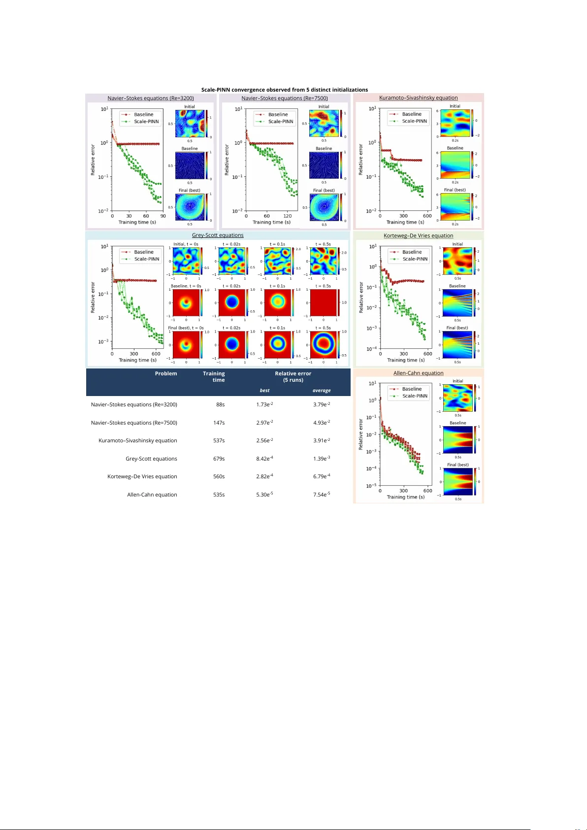
Scale-PINN: Learning Eﬃcien t Ph ysics-Informed Neural Net w orks Through Sequen tial Correction P ao-Hsiung Chiu 1 † , Jian Cheng W ong 1* † , Chin Ch un Ooi 1,2 , Chang W ei 3 , Y uchen F an 3 , Y ew-So on Ong 2,4 1 Institute of High P erformance Computing, A*ST AR, Singap ore. 2 Cen tre for F ron tier AI Research, A*ST AR, Singap ore. 3 Sc ho ol of Mec hanical Engineering, Tianjin Universit y , China. 4 College of Computing and Data Science, Nan yang T echnological Univ ersit y , Singap ore. *Corresp onding author(s). E-mail(s): w ong j@a-star.edu.sg ; Con tributing authors: chiuph@a-star.edu.sg ; ooicc@a-star.edu.sg ; w ei c hang@tju.edu.cn ; fanyuc hen@tju.edu.cn ; asysong@n tu.edu.sg ; † These authors con tributed equally to this work. Abstract Ph ysics-informed neural net w orks (PINNs) ha v e emerged as a promising mesh-free paradigm for solving partial diﬀeren tial equations, yet adoption in science and engineer- ing is limited by slow training and modest accuracy relative to mo dern numerical solvers. W e introduce the Sequen tial Correction Algorithm for Learning Eﬃcient PINN (Scale- PINN), a learning strategy that bridges mo dern ph ysics-informed learning with n umerical algorithms. Scale-PINN incorp orates the iterative residual-correction principle, a corner- stone of numerical solvers, directly into the loss formulation, marking a paradigm shift in ho w PINN losses can b e conceived and constructed. This integration enables Scale- PINN to achiev e unpreceden ted conv ergence sp eed across PDE problems from diﬀerent ph ysics domain, including reducing training time on a c hallenging ﬂuid-dynamics prob- lem for state-of-the-art PINN from hours to sub-2 minutes while maintaining sup erior accuracy , and enabling application to representativ e problems in aero dynamics and urban science. By uniting the rigor of numerical metho ds with the ﬂexibility of deep learning, Scale-PINN marks a signiﬁcant leap to w ard the practical adoption of PINNs in sci- ence and engineering through scalable, physics-informed learning. Co des are a v ailable at h ttps://github.com/c hiuph/SCALE- PINN . Keyw ords: Physics-informed neural net works, sequen tial correction algorithm, loss function, PINN benchmark, ﬂuid-dynamics 1 In tro duction Ph ysics-Informed Neural Net w orks (PINNs) ha v e emerged as a promising paradigm for solving partial diﬀerential equations (PDEs) by em b edding gov erning physics into the training loss. Their mesh-free nature, abilit y to in tegrate ph ysics with sparse data, and suitabilit y for inv erse problems ha ve sparked widespread in terest across computational science, from ﬂuid and solid mec hanics to electromagnetism, optics, earth sciences, materials science, electro c hemistry , and 1 epidemiology , underscoring their growing prominence as an alternative to n umerical sim ulation metho ds [ 1 – 7 ]. Ho wev er, a key limitation of PINNs thus far, even when employing improv ed neural arc hitectures and state-of-the-art learning strategies [ 8 – 12 ], is their high computational cost- accuracy trade-oﬀ. First, the use of dense training samples and large batc h sizes improv es accuracy but signiﬁcan tly increase computational demands. Second, adaptiv e sampling and neural tangen t kernel-based adaptive loss w eighting metho ds in tro duce considerable o verhead to ov ercome spectral bias and complex loss landscap e issues. Third, the need for curriculum and sequence-to-sequence training to gradually reﬁne the solution from an initial guess to prev ent premature con vergence is v ery costly in more complex problems, suc h as stiﬀ and m ulti-scale PDEs. F ourth, some studies hav e turned to second-order optimization metho ds, including BFGS algorithm and Quasi-Newton v arian ts, to improv e accuracy through more precise updates. All of them substantially increase the computational costs as a trade-oﬀ for ac hieving quality outcome. As a result, PINN training is muc h slo wer than numerical solv ers, limiting their broader adoption in real-w orld scientiﬁc and engineering problems [ 13 ]. Curi- ously , these strategies derive primarily from the general machine learning literature and do not leverage insights from scientiﬁc computing. In seeking to ov ercome this limitation, w e recognize that the scientiﬁc computing commu- nit y has dev elop ed a w ealth of knowledge and algorithmic tec hniques o ver the past decades for eﬃcien tly solving complex PDEs—many of whic h can b e p oten tially adopted to adv ance PINN methodologies. F or example, realizing that lac k of neigh b orhoo d dependencies infor- mation may lead to training failure, numerical diﬀerentiation techniques, including the ﬁnite diﬀerence, ﬁnite v olume and ﬁnite elemen t discretizations, ha ve b een employ ed to successfully enhance physics-informed learning b y enforcing lo cal spatial coupling [ 14 – 19 ]. F urthermore, com bining automatic diﬀerentiation and numerical discretization for PINNs has prov en eﬀec- tiv e in impro ving both accuracy and computational eﬃciency [ 20 , 21 ]. The artiﬁcial eddy viscosit y and pseudo-time stepping methods are other notable examples for impro ving training stabilit y [ 22 – 24 ]. These early successes highlight a promising direction of integrating algo- rithmic insights from scientiﬁc computing into PINN for designing practical and scalable ph ysics-informed learning framew orks. While these developmen ts demonstrate the p o wer of infusing discretization wisdom into the PINN framework, they hav e largely drawn from only one of the tw o pillars of numerical sim ulation: discretization and iterativ e metho d. Modern n umerical methods not only discretize go verning equations but also solv e the resulting linear systems through carefully designed iter- ativ e sc hemes that guaran tee con vergence, stabilit y , and precision. Building on this foundation, w e demonstrate that the second pillar—iterativ e schemes—can b e a rich source of algorithmic insigh t for eﬃcient ph ysics-informed learning. In this w ork, we establish that iterativ e resid- ual correction, whic h is a principle at the core of many n umerical solvers, can b e explicitly realized within the PINN loss formulation with remark able gains in PINN learning. Our proposed Sequential Correction Algorithm for Learning Eﬃcien t PINN (Scale-PINN) em b odies this idea: b y em b edding a sequential correction mechanism within the training pro- cess through an auxiliary loss function, Scale-PINN achiev es b oth speed and sample eﬃciency . This persp ectiv e marks a paradigm shift in ho w PINN losses are conceiv ed and constructed, b y dra wing on the foundations of iterativ e methods that hav e long pow ered scientiﬁc com- puting. The inherently iterativ e nature of these up dates aligns seamlessly with the curren t state-of-the-art mini-batc h sto c hastic gradient descen t (SGD) optimizers. On representativ e stiﬀ-conditioned lid-driven cavit y b enc hmarks, Scale-PINN reaches a target accuracy of rela- tiv e error ≤ 2 e -2 in sub-2 minutes, compared with 15 hours for prior state-of-the-art training strategies [ 12 ], and attains impro ved accuracy . A schematic diagram of Scale-PINN is illus- trated in Fig. 1 . Our prop osed framew ork is generic and easy to implemen t with broad applicabilit y to domains suc h as aero dynamics and urban science, and it op ens new possibilities for tackling practical problems in computational science with PINNs. 2 Na v i e r – S t o k e s e q ua t i o ns    +          +    +   = 0   +          +    +   = 0   +   = 0 L id - d ri v e n c a v i t y f l o w , R e =3200 ( t r ai n i n g t i m e ~ 9 0 s ) L id - d ri v e n c a v i t y f l o w , R e =7500 ( t r ai n i n g t i m e ~ 1 5 0 s ) S cal e - P I NN sch em at i c  x t I np ut v a r ia b le s f   I n it ia l c o n d it io n / b ou n d a r y c on d i t i on      D if f e r e n t ia l e q u a t i on    =  I C/ B C l o s s P D E lo ss ac t i v at i on:   = si n    Fr eq u en c y a nne a l i ng S olv e d b y it e r at iv e op t i m i z at ion ( e . g . , S G D ) :     =        +          +               =       S eq u en t i a l c o r r ec t i o n t er m ( e. g . , H e lm h o lt z r e sid u a l sm o o t h in g o p e r a t o r )     =              =       +        M in i m iz at i on : G re y - S c o tt e q u a ti o n s    0 . 2   +     4 0 1   + 1 0 0 0    = 0    0 . 1   +    + 1 0 0   1 0 0 0    = 0 A lle n - Cah n e q u at i o n    0 . 0 0 0 1   + 5     = 0 K u ra mo t o – S iv a sh in sk y e q u a t i on   + 1 0 0 1 6    + 1 0 0 1 6    + 1 0 0 1 6    = 0 Ko r t e we g – D e V r ie s e q u a t io n   +    + 0 . 0 2 2    = 0 S cal e - P I N N co n v er g en ce v s. n u m er i cal so l v er on s ol v i ng l i d - dr i v e n c a v i t y f l ow ( R e = 3200) Fig. 1 Scale-PINN schematic and result highligh ts. Scale-PINN includes a sequential correction term through application of the residual smo othing operator P α = ( I − α 2 ∇ 2 ) to the change in solution F : = f ( · ; w k ) − f ( · ; w k − 1 ) during iterativ e optimization. A conv ergence plot on the Na vier-Stokes (N-S) example, lid-driven cavit y ﬂow at Re = 3200, shows comp etitiv e time-to-accuracy v ersus n umerical solv ers. Compared to other PINN metho ds, Scale-PINN solv es the lid-driven cavit y ﬂow to state-of-the-art accuracy with unprecedented speed, i.e., ∼ 90s for Re = 3200 and ∼ 150s for Re = 7500. Results for Kuramoto–Siv ashinsky (K-S), Grey–Scott (G-S), Korteweg–De V ries (KdV), and Allen–Cahn (AC) equations demonstrate accuracy across div erse dynam- ics. Scale-PINN model architecture and training strategies are detailed in Method 4.5 . 2 Results 2.1 Sequen tial correction algorithm for learning eﬃcien t PINN mo dels W e in tro duce Scale-PINN as a neural PDE solv er for scien tiﬁc simulations, emphasizing its capabilit y to predict physical outcomes in fully sp eciﬁed systems gov erned by PDEs and the prescribed initial conditions (IC) and boundary conditions (BC). By reformulating the sim ulation as a ph ysics-informed learning task, we seek to optimize the netw ork weigh ts w suc h that the output function f satisﬁes the requisite PDE constraints. The ob jective (loss) function for PINN w eight parameters optimization can b e expressed as L ( w ) = L pde + λ ic L ic + λ bc L bc whic h comprises contributions from the PDE, ICs, and 3 BCs (see Metho d 4.1 ). Among the three loss comp onen ts, the gov erning PDE loss, L pde = ∥N ϑ [ f ( · ; w )] − h ( · ) ∥ 2 L 2 (Ω × (0 ,T ]) (1) greatly aﬀect the PINN training diﬃculty . Highly nonlinear PDEs, such as the Na vier-Stokes (N-S) equations, often exhibit steep gradients and strong interactions among v ariables. This mak es it diﬃcult for PINNs to satisfy all gov erning equations simultaneously . Moreo v er, small training p erturbations can substan tially c hange the PDE dynamics across the domain, hinder- ing conv ergence to the correct solution. These factors, in addition to the high dimensionality and non-linear characteristics of neural net works, contribute to a rugged PDE loss landscape, resulting in multiple lo cal minima, oscillatory optimization paths, and hence a higher likelihoo d of b ecoming trapped in sub optimal solutions [ 25 ]. PINN training is commonly performed using iterative optimization methods, suc h as SGD and Adam algorithms. They progressiv ely evolv e the weigh t parameters from an initial guess w 0 , ov er man y iterations along the descen t direction of the loss function w k +1 = w k − η ∇L ( w k ) (2) where the curren t iteration num b er k is denoted in superscript, and η is a problem-dep enden t learning rate. This approac h, often implemen ted via mini-batch training, exploits a v arying set of sample p oin ts for loss (and gradien t) ev aluation at each iteration. In the context of PINNs, training with incomplete and contin uously changing system information in tro duces an addi- tional la yer of instability , amplifying optimization oscillations and making stable con vergence in a complex loss landscap e more diﬃcult. Mathematically derived from the iterativ e scheme (see Metho d 4.2 for details), we propose Scale-PINN b y introducing a sequential correction term (auxiliary sequence) F at iteration k > 0, which mo diﬁes the PDE loss term L pde to improv e con vergence: L k sc-p de = ∥N ϑ [ f ( · ; w k )] − h ( · ) + 1 τ sc F ∥ 2 L 2 (Ω × (0 ,T ]) (3a) F = B ( f ( · ; w k ) − f ( · ; w k − 1 )) (3b) τ sc is the hyperparameter. The matrix B constitutes a key design element of the iterative framew ork, as it determines the operator used in the up date. B can b e ﬂexibly selected to reﬂect problem-dep enden t structure or to promote sp eciﬁc solution prop erties. The standard PINN loss function is obtained as the limiting case B = 0. In present study , we instan tiate B ≡ P α = ( I − α 2 ∇ 2 ) as the residual smo othing operator applied to the c hange in solution f ( · ; w k ) − f ( · ; w k − 1 ) during iterativ e optimization. W e sho w equiv alence to the implicit residual smo othing method (see Metho d 4.3 for details), with asso ciated enhanced stability and reduced oscillation during training. L sc-p de from equation ( 3 ) can then b e recast as: L k sc-p de = ∥N ϑ [ f ( · ; w k )] − h ( · ) + 1 τ sc F − γ τ α ∇ 2 F ∥ 2 L 2 (Ω × (0 ,T ]) = ∥N ϑ [ f ( · ; w k )] − h ( · ) + ( M f − M v ) ∥ 2 L 2 (Ω × (0 ,T ]) (4a) M f = 1 τ sc f ( · ; w k ) − γ τ α ∇ 2 f ( · ; w k ) (4b) M v = 1 τ sc f ( · ; w k − 1 ) − γ τ α ∇ 2 f ( · ; w k − 1 ) (4c) with tunable hyperparameters τ sc > 0, γ > 0, and τ α > 0 ( α 2 = τ sc γ τ α ). Diﬀeren t from standard PDE loss, tw o additional auxiliary terms, i.e., stabilization term M f (residual smoothing op erator) and consistency term M v (coun ter term comp ensates for the inclusion of M f ), are in tro duced to enhance the PINN training b eha vior as w ell as ensure 4 the ﬁnal solution will con verge to original system. Equation ( 4 ) is straigh tforward to imple- men t, as the auxiliary terms in M f are already computed for the standard PDE loss. The new required operations are storing of the netw ork weigh ts from the previous iteration, w k − 1 , p erforming a forw ard pass to compute f ( · ; w k − 1 ), and conducting tw o bac kward passes to ev aluate ∇ 2 f ( · ; w k − 1 ) on the latest iteration mini-batc h samples, all of which incur negligible additional computational o verhead during training. Algorithm 1 (Method 4.3 ) summarizes the o verall computational procedure of the Scale-PINN, which in tegrates seamlessly with widely used iterative optimization methods such as SGD and Adam. 5 it e r a t io n s 500 i t e ra t i o n s 5 k it e r a t io n s 50 k it e r a t io n s 500 k it e r a t io n s 5 it e r a t io n s 500 i t e ra t i o n s 5 k it e r a t io n s 50 k it e r a t io n s 500 k it e r a t io n s 5 it e r a t io n s 500 i t e ra t i o n s 5 k it e r a t io n s 50 k it e r a t io n s 500 k it e r a t io n s 5 it e r a t io n s 500 i t e ra t i o n s 5 k it e r a t io n s 50 k it e r a t io n s Tr ai n i n g t i me ~780s ( a ) L i d - d r iv e n c a v it y f lo w , R e = 4 0 0 Tr ai n i n g t i me ~1800s Tr ai n i n g t i me ~1800s Tr ai n i n g ti m e ~90s P I NN ( tr a i ni ng ti m e ~1800s ) S cal e - P I NN ( tr a i ni ng ti m e ~90s ) 5 it e r a t io n s 1 k it e r a t io n s 5 k it e r a t io n s 10 k it e r a t io n s 50 k it e r a t io n s 5 it e r a t io n s 10 k it e r a t io n s 50 k it e r a t io n s 100 k it e r a t io n s 500 k it e r a t io n s ( b ) L i d - d r iv e n c a v it y f lo w , R e = 3 2 0 0 S cal e - P I NN ( tr a i ni ng ti m e ~90s ) PI N N ( tr a i ni ng ti m e ~1800s ) Fig. 2 (a) Exp erimen tal analysis on lid-driven cavit y ﬂow at Re = 400 sho ws that the conv ergence of a v anilla PINN can be impro ved by increasing batch size (400 → 4,000) and reducing learning rate (1e -3 → 1e -4 ), albeit at a slo wer pace ( ∼ 1800s). Scale-PINN requires substan tially less training iterations to reach orders of magnitude higher accuracy ( ∼ 90s), while using 1 order of magnitude smaller batch size and higher learning rate. Comparing their intermediate ﬂow ﬁelds progressing from a few iterations to 50 k -500 k iterations, and mid-section proﬁles against the Ghia et al. [ 26 ] benchmark, Scale-PINN attains accurate ﬂow structures far earlier. (b) Scale-PINN can conv erge to an accurate solution even when the Reynolds num ber is increased to Re = 3200, without the need to increase batc h size and n umber of training iterations. A v anilla PINN struggles to solve the Re = 3200 case, as it b ecomes trapp ed in incorrect ﬂow patterns, indicating premature con vergence. 2.2 Eﬃcien t scientiﬁc sim ulation with Scale-PINN W e demonstrate Scale-PINN on a classical b enc hmark problem in computational ﬂuid dynam- ics (CFD), the lid-driven ca vity ﬂow (Metho d 4.4.1 ). The ﬂuid ﬂow inside a 2D unit square, x ∈ [0 , 1], y ∈ [0 , 1], is driv en b y the top lid v elo cit y ( u lid = 1), and gov e r ned by the steady-state incompressible N-S equations for velocity  u = [ u, v ] ⊺ and pressure p : ∇ ·  u = 0 (5a) (  u · ∇ )  u = 1 Re ∇ 2  u − ∇ p (5b) 5 Complex ph ysical phenomenon can b e observed when the Reynolds num b er ( Re ) increases, suc h as Re ≥ 3200, making it notoriously diﬃcult for PINN metho ds to solve (e.g., require hours to tens of hours of training) even with the help of some labeled data or transfer and curriculum learning [ 10 , 11 ]. In con trast, Scale-PINN is fast and eﬀectiv e at tackling this v ery c hallenging PINN benchmark problem (see results highlighted in Fig. 1 -Fig. 3 ). Building on equation ( 4 ) as per the Scale-PINN metho dology , the loss function for momen tum equations ( 5b ) can be deﬁned as b elo w: L k sc-p de(Mu) = ∥ u k ∂ u k ∂ x + v k ∂ u k ∂ y − 1 Re ( ∂ 2 u k ∂ x 2 + ∂ 2 u k ∂ y 2 ) + ∂ p k ∂ x + S Mu ∥ 2 L 2 (Ω) (6a) L k sc-p de(Mv) = ∥ u k ∂ v k ∂ x + v k ∂ v k ∂ y − 1 Re ( ∂ 2 v k ∂ x 2 + ∂ 2 v k ∂ y 2 ) + ∂ p k ∂ y + S Mv ∥ 2 L 2 (Ω) (6b) S Mu = 1 τ sc ( u k − u k − 1 ) − γ uv τ α " ( ∂ 2 u k ∂ x 2 + ∂ 2 u k ∂ y 2 ) − ( ∂ 2 u k − 1 ∂ x 2 + ∂ 2 u k − 1 ∂ y 2 ) # (6c) S Mv = 1 τ sc ( v k − v k − 1 ) − γ uv τ α " ( ∂ 2 v k ∂ x 2 + ∂ 2 v k ∂ y 2 ) − ( ∂ 2 v k − 1 ∂ x 2 + ∂ 2 v k − 1 ∂ y 2 ) # (6d) with the integration of sequen tial correction terms S Mu and S Mv as deﬁned by the c hoice of the Helmholtz residual smoothing op erator ( P α = ( I − α 2 ∇ 2 )). In this study we set γ uv = 1 Re based on prior knowledge of the go verning ph ysical system. V alues of τ sc and τ α are ﬁne-tuned empirically . A fundamen tal diﬃculty in solving incompressible N-S equations is that the pressure v ari- able do es not app ear explicitly in the con tinuit y equation and only app ears through its gradien t in the momen tum equations [ 27 , 28 ]. Th us, several numerical schemes prop osed to modify the con tinuit y formulation to relax the incompressibility constrain t by explicitly establishing a dynamic relationship betw een pressure and contin uity [ 28 – 30 ]. Guided by the same principle, the Scale-PINN loss function for the contin uity equation ( 5a ) is deﬁned as follows: L k sc-p de(Cn) = ∥ ∂ u k ∂ x + ∂ v k ∂ y + S Cn ∥ 2 L 2 (Ω) (7a) S Cn = 1 τ sc ( p k − p k − 1 ) (7b) Scale-PINN allows S Cn to b e introduced in to the con tinuit y loss term to explicitly provide a relation betw een pressure and the contin uit y equation, thereby improving conv ergence. T ogether with a BC loss term L bc to enforce the top lid velocity u lid = 1, v lid = 0 and no- slip w all condition u = v = 0, the Scale-PINN ob jective function for simulating the lid-driv en ca vity ﬂo w is thus deﬁned as: L sc ( w k ) = L k sc-p de(Mu) + L k sc-p de(Mv) + L k sc-p de(Cn) + λ bc L k bc . Our exp erimen tal analysis (Fig. 2 ) suggests that the principal barrier for v anilla PINNs is not merely insuﬃcient compute but an unstable optimization landscape. A t R e = 400, with a small batch size and large learning rate, the conv ergence is slo w (ov er 500 k iterations, training time ∼ 780s) and susceptible to premature lo c king into sub optimal ﬂo w patterns. Increasing the batch ten-fold (400 → 4,000) and reducing the learning rate ten-fold (1e -3 → 1e -4 ) stabilizes conv ergence, but it also leads to signiﬁcan tly increased training time ( ∼ 1800s). In con trast, Scale-PINN attains m uch lo wer error (MSE < 1e -5 ) in only 50 k iterations (training time ∼ 90s) using the smaller batch and larger learning rate. Visual snapshot across training iterations show that Scale-PINN resolv es the primary vortex and corner eddies earlier, and its mid-section u - and v -proﬁles match the classical Ghia et al. [ 26 ] cut-lines, indicating ph ysically faithful pressure-velocity coupling. A t Re = 3200, Scale-PINN con tinues to conv erge without increasing batc h size or iteration budget, whereas v anilla PINN becomes trapp ed in incorrect lo cal minima. These con trast supp orts our in terpretation that the sequential correction in Scale-PINN eﬀectively smo oths the PDE residuals, enabling steady progress with standard ﬁrst-order optimizers. The cross-regime results summarized in Fig. 3 (a) underscore that Scale-PINN not only attains state-of-the-art accuracy but also establishes a new b enc hmark in eﬃciency across an unpreceden ted range of Reynolds num b ers. Scale-PINN remains both accurate and fast from 6 R e = 4 0 0 R e = 3 2 0 0 R e = 7 5 0 0 R e = 1 0 k R e = 2 0 k M SE 8 . 9 8 e - 6 1 . 4 8 e - 5 4 . 2 9 e - 5 3 . 4 3 e - 5 9 . 3 9 e - 5 R el a t i v e er r o r 1 . 4 3 e - 2 1 . 7 3 e - 2 2 . 9 7 e - 2 2 . 7 4 e - 2 4 . 4 3 e - 2 T r a in in g t im e ( s ) l e ss t ha n 9 0 9 0 1 5 0 3 6 0 3 8 0 N o . it e r a t io n s 5 0 , 0 0 0 5 0 , 0 0 0 5 0 , 0 0 0 8 0 , 0 0 0 1 0 0 , 0 0 0 I n it ia l le a r n in g r a t e 1 e - 3 5 e - 4 5 e - 4 5 e - 4 5 e - 4 B a t c h s i ze / i t er . 4 0 0 4 0 0 1 , 0 0 0 2 , 0 0 0 2 , 4 0 0 N o . t r a in in g sa mp l e 1 0 0 x 1 0 0 1 0 0 x 1 0 0 1 5 0 x 1 5 0 2 5 6 x 2 5 6 2 5 6 x 2 5 6 N e t w or k s i z e ( no . p a r a m et er s ) 1 5 , 4 2 4 1 5 , 4 2 4 5 9 , 5 2 0 5 9 , 5 2 0 5 9 , 5 2 0 L id- dr iv e n c a v it y f lo w , R e = 2 0 k ( tr a i ni ng ti m e ~380s ) L id- dr iv e n c a v it y f lo w , R e = 4 0 0 ( tr a i ni ng ti m e ~90s ) u - v e lo c it y v - v e lo c it y L id- dr iv e n c a v it y f lo w , R e = 1 0 k ( tr a i ni ng ti m e ~360s ) (a) S c al e - P I N N p e rf o rm a n ce a cro s s re g i m e s o f i n cre a s i n g co m p l e x i t y f o r l i d - d r iv e n c a v it y f lo w ( R e = 4 0 0 – 2 0 k ) ( b ) C o n v e r g e n c e o f S c a l e - P INN v s . o t h e r P INN m e t h o d s f o r l i d - d r iv e n c a v it y f lo w ( R e = 3 2 0 0 ) ( c ) S c a l i n g b e h a v i o u r o f d i f f e r e n t P I N N m e th o d s a s p r o b l e m c o m p l e xi ty i n c r e a s e s S cal e - P I NN [ R T X 3090] We i et a l . ( 2 0 2 5 ) [ R T X 3090] Wa n g et a l . ( 2 0 2 4 ) r e pr o duc e d in - ho us e [ R T X 3090] Wa n g et a l . ( 2 0 2 5 ) R e =5000 [ A 6000] Wo n g e t al . ( 2 0 2 3 ) r e pr o duc e d in - ho us e [ R T X 3090] K h a de m i & D u f o u r ( 2 0 2 5 ) da ta +phy s i c s T s a i e t al . ( 2 0 2 5 ) R e =5000 [ R T X 4070 - TS ] Wa n g et a l . ( 2 0 2 4 ) R e =3200 Wa n g et a l . ( 2 0 2 4 ) R e =400 Wo n g et a l . ( 2 0 2 3 ) R e =3200 Wo n g et a l . ( 2 0 2 3 ) R e =400 S cal e - PI N N R e =3200 S cal e - PI N N R e =400 Fig. 3 (a) Scale-PINN solves the lid-driven ca vity ﬂo w from Re = 400 to R e = 20 k with state-of-the-art accuracy and eﬃcient training, as shown in the summary table of error, training time, and other parameters, alongside the represen tative v elo cit y ﬁelds and absolute error maps ( Re = 400 and Re = 20 k ) to conﬁrm that residuals remain small and largely conﬁned to shear lay ers and vortex cores. F or all simulated cases, their MSE consistently b elo w 1e -4 , and their mid-section u and v -v elo cit y proﬁles (colored lines) sho w excellen t agreement with the classic benchmark results (marked points) for n umerical solvers, i.e., Ghia [ 26 ] for up to Re = 10 k and Erturk [ 31 ] for R e = 20 k . (b) Scale-PINN establishes a sub-2 minutes training regime on lid-driv en ca vity ﬂow ( Re = 3200), whereas recen t PINN v ariants require hours to approach comparable accuracy . (c) Scale-PINN scales fav orably with problem complexity ( Re : 400 → 3200), enabling the solution of more complex problems within a feasible time scale. Re = 400 to Re = 20 k , with relativ e error rising only mo destly (1.4e -2 → 4.4e -2 ) as the problem complexit y increases (learning stiﬀness in tensiﬁes), while training time stays under seven min- utes ( ∼ 380s) even at Re = 20 k . Scale-PINN demonstrates fa vorable scaling of optimization cost with problem complexity , despite deliberately increased resolution (100 2 → 256 2 ), batch size (400 → 2400), and num b er of iterations (50 k → 100 k ) to resolv e thinner b oundary lay ers and 7 stronger shear at higher Reynolds n umber. F or all sim ulated cases, their mid-section u and v -v elo cit y proﬁles show excellent agreemen t with canonical b enc hmarks (Ghia et al. [ 26 ] up to Re = 10 k and Erturk [ 31 ] at Re = 20 k ), thereb y demonstrating, for the ﬁrst time, that a PINN approac h can deliver accurate and eﬃcient N-S solutions at the high-Reynolds regime. The results highligh t Scale-PINN as a scalable method across regimes, with predictions consisten t with established numerical standards. W e b enc hmark Scale-PINN against recent PINN metho ds at Re = 3200, which fea- tures in several state-of-the-art PINN literature as a challenging regime, where man y PINNs fail to conv erge. W e include metho ds whose original pap er rep orts successfully solving the problem with relative error b elo w 1e -1 : W ong et al. (2023, LSA-PINN) [ 32 ], W ang et al. (2024, PirateNets) [ 11 ], Khademi & Dufour (2025, TSA-PINN) [ 33 ], and W ei et al. (2025, FFV-PINN) [ 34 ]. LSA-PINN and PirateNets are reproduced in-house on a single R TX 3090 (Scale-PINN trained on the same hardw are) using av ailable source co de. W e also include Re = 5000 results from W ang et al. (2025, SOAP) [ 12 ], a second-order optimizer and successor to PirateNets, and Tsai et al. (2025, MLD-PINN) [ 35 ], because they disclose timing; this oﬀers a useful sp eed-accuracy reference despite the higher Reynolds n umber. As shown in Fig. 3 (b), Scale-PINN’s sub-2 minutes training regime represen ts a new state-of-the-art speed-accuracy P areto fron tier for Re = 3200. Scale-PINN is trained from scratch, i.e., He initialization [ 36 ], without pre-training, curriculum sc hedules, or data sup ervision. Con temp orary PINN v ariants are often aided b y curriculum strategies (e.g., Re : 100 → 400 → 1000 → ... → 3200) [ 11 , 12 ], n umer- ical diﬀerentiation loss [ 32 , 34 , 35 ], or additional data sup ervision [ 33 ], and many of them still require hours of training to approach comparable prediction accuracy . Fig. 3 (c) illustrates the con vergence b eha vior of Scale-PINN relative to other metho ds as the problem complexity increases ( Re : 400 → 3200). Scale-PINN maintains excellent con ver- gence speed and accuracy across regimes. In con trast, LSA-PINN training increases from less than 10 min utes to more than 1 hour, accompanied b y a signiﬁcant degradation in accuracy , while PirateNets requires up to 12-15 hours to achiev e comparable accuracy . This con trast highligh ts the sup erior scalabilit y of Scale-PINN: as the problem b ecomes more challenging, its con vergence sp eed degrades far more slowly than competing metho ds, enabling the solution of increasingly complex ﬂuid dynamics problems within feasible computational budgets. The impressiv e impro vemen ts in Scale-PINN training regime motiv ate, for the ﬁrst time in a PINN study , direct comparisons with high-ﬁdelit y CFD solvers. W e compare Scale-PINN against an in-house CFD solver [ 37 ], whic h has b een demonstrated to pro duce high-ﬁdelity solutions for the incompressible N-S equations, and the widely-used commercial solv er Ansys Fluen t, recognized for its reliabilit y , generality , and parallel p erformance. W e ﬁrst run the in-house solver on a 96 × 96 mesh and record the runtime and accuracy along the con vergence tra jectory . Given a runtime of around 80s, Scale-PINN ac hieves higher con verged accuracy (Fig. 1 ), establishing a new sp eed-accuracy Pareto frontier. W e then utilize similar sim ulation settings in Fluent on a ﬁner 128 × 128 mesh. Its conv erged accuracy is m uch p oorer than b oth the in-house co de (on 96 × 96 mesh) and Scale-PINN. Finally , w e p erform the sim ulations on a muc h ﬁner 192 × 192 mesh using four CPU cores for b oth Fluent and the in- house co de. With the optimized parallelization, results from Fluen t no w match our metho d’s accuracy in around 120s run time. The in-house solver, with a basic OpenMP implemen tation, to ok nearly twice as long to achiev e the same accuracy , although it should b e ackno wledged that it can even tually reach the highest accuracy with additional run time. These comparisons suggest that mesh-free PINN methods may b e well s u ited for practical scien tiﬁc and engineering problems under ﬁxed computational budgets. In scientiﬁc computing, practitioners often choose the coarsest mesh that delivers ph ysics-resolved accuracy , balancing ﬁdelit y against cost; ac hieving higher accuracy t ypically requires ﬁner meshes and substan- tially more compute. Lev eraging theoretically exact automatic diﬀerentiation for deriv ative ev aluation, Fig. 1 sho ws that Scale-PINN can outp erform a con v entional second-order n umer- ical scheme as employ ed b y Fluen t on a relatively coarse mesh (e.g., 128 × 128). In practical terms, under a limited time budget, Fluent on a 128 × 128 mesh yields the b est accuracy within ∼ 30s runtime; Scale-PINN pro vides the b est accuracy within ∼ 120s; and if runtime is unconstrained, the in-house solver on a ﬁne mesh achiev es the highest accuracy . 8 2.3 Na vier–Stok es ﬂow sim ulation for engineering and urban science ( b ) F l o w p a s t s ta g g e r e d a ir f o ils , R e = 5 0 0 (a) F l o w p as t a ir f o il , R e = 1 0 0 0 Fig. 4 Scale-PINN predictions, with streamlines ov erlaid on velocity magnitude contours, for ﬂo w past (a) a single-airfoil at Re = 1000 and (b) staggered airfoils at Re = 500 are compared to reference solutions obtained from CFD. Component-wise ﬁelds ( u , v , p ) and absolute error maps indicate goo d agreement b et w een Scale- PINN and CFD across the domain, including wak es b ehind airfoil. Surface pressure-coeﬃcient ( C p ) traces along the airfoil(s) closely match CFD and literature curves. Only the near-ﬁeld region is shown for clarity , where the ﬂo w patterns around the airfoil(s) emerge; the actual computational domain extends well b ey ond the visualized region. Scale-PINN reac hes accurate solutions within ∼ 180s of training, achieving near-ﬁeld velocity relative errors of 1 . 7 e -2 (3 . 47 e -3 full domain) for the single-airfoil case and 1 . 96 e -2 (4 . 79 e -3 full domain) for the staggered airfoils case. These results v alidate the accuracy and eﬃciency of Scale-PINN in resolving canonical aerodynamic ﬂow features at moderate Reynolds num b er. T o demonstrate the applicabilit y b ey ond lid-driv en cavit y b enc hmarks, we present Scale- PINN results on t wo represen tative aerodynamic problems: (1) ﬂow past a single NACA0012 airfoil at Re = 1000 and 7 ◦ angle of attac k (AoA); and (2) ﬂo w past tw o-staggered NA CA0012 airfoils at Re = 500 and 7 ◦ AoA (Metho d 4.4.1 ). NA CA airfoil problems are classical b enc h- marks, where fast and reliable ﬂow simulations are crucial for adv ancing the design and optimization of aero dynamic structures suc h as aircraft and wind turbines. F or the single-airfoil case, Scale-PINN predictions produce the exp ected wak e patterns (Fig. 4 a) and show excellen t agreement b et w een comp onen t-wise velocity ( u , v ) and pressure ( p ) ﬁelds and CFD reference solutions. Even for the more complex scenario of tw o-staggered airfoils, Scale-PINN successfully captures the altered w ake structures and aerodynamic inter- actions b et w een the b o dies, with predicted v elo cit y and pressure ﬁelds aligning well with CFD (Fig. 4 b). F or both cases, absolute error maps indicate that minor and localized discrepancies are mainly conﬁned within the leading edge and near-w ake regions. The pressure coeﬃcient ( C p ) distribution along the airfoil surfaces compare well with b oth CFD and literature data from Kurtulus [ 38 ], even capturing the suction p eak at the leading edge and subsequen t pressure recov ery . 9 Scale-PINN requires only ∼ 180s of training to pro duce solutions in excellent agreemen t with CFD ground truth. In contrast, Xiao et al. [ 39 ] rep ort a training time of ∼ 7800s and the need for additional sensor p oin ts to ac hieve comparable accuracy for airfoil ﬂows, high- ligh ting the sup erior eﬃciency and accuracy of Scale-PINN. Scale-PINN demonstrates robust p erformance across b oth single-bo dy conﬁgurations and multi-bo dy aerodynamic in teractions, underscoring its p oten tial for aero dynamic design and optimization with multi-elemen t airfoils. ( a ) F lo w p a s t s q u a r e c y lin d e r s , R e = 2 5 ( b ) R a y le ig h - B é n ar d c o n v e c t io n , R a = 1 0 0 k Fig. 5 (a) Scale-PINN sim ulates the ﬂow past square cylinders in op en domain, where the predicted ﬁelds ( u , v , p ) accurately capture the wak e structure and recirculation zones, with consistently low absolute errors against the reference solution obtained from CFD. Con tours are shown in the near ﬁeld for clarit y; the actual com- putational domain extends further. Scale-PINN reaches accurate solutions within ∼ 285s of training, ac hieving near-ﬁeld velocity relative errors of 9 . 21 e -3 (4 . 86 e -3 full domain). (b) Scale-PINN sim ulates Rayleigh–B ´ enard conv ection at Ra = 100 k . The temp erature contours, overlaid with v elo cit y streamlines, sho w close agreement between predicted roll patterns and reference solutions obtained from CFD, across multiple time snapshots (1- 50s). Scale-PINN achiev es accurate solutions within ∼ 390s of training, with relativ e errors 1 . 99 e -2 for v elo cit y and 3 . 2 e -2 for temp erature. These cases v alidate the metho d’s robustness across bluﬀ-b ody geometries in op en domain and thermally driv en, time-dep enden t conv ection. W e next sim ulate ﬂow past three staggered square cylinders at Re = 25, a canonical pro xy for wind ﬂow around buildings (Metho d 4.4.1 ). Scale-PINN accurately reco vers wak e structures and recirculation zones, with v elo cit y and pressure ﬁelds closely matc hing CFD references and errors conﬁned to shear la yers and separation points (Fig. 5 a). These results conﬁrm Scale-PINN’s robustness for bluﬀ-bo dy aero dynamics in op en domains, where reliable prediction of ﬂow interactions are commonly used to inform urban ven tilation design and p ollutan t disp ersion. 10 W e further v alidate Scale-PINN on buo yancy-driv en Ra yleigh–B ´ enard con vection at Ra = 100 k to demonstrate its v ersatility in mo deling multiph ysics transient dynamics, where ther- mal instabilities give rise to conv ection rolls and their transien t ev olution in to complex patterns (Metho d 4.4.1 ). Scale-PINN predictions remain in close agreement with CFD b enc hmarks across m ultiple time snapshots b et w een 1s and 50s, with lo w residuals sustained ov er time (Fig. 5 b). By capturing the onset and developmen t of natural conv ection, Scale-PINN demon- strates its capacity to mo del thermally-driv en ﬂows of direct imp ortance to energy eﬃciency , v entilation, and thermal comfort in the built environmen t and urban sustainability studies. Our results further conﬁrm the sup erior sampling p oin ts (or mesh ﬁdelit y) to accuracy trade-oﬀ enabled b y Scale-PINN (relativ e to CFD). With temp oral step size of 0.001, CFD solution achiev es an MSE of 4 . 0 e -5 and 3 . 32 e -5 for temp erature and v elo cit y magnitude, respec- tiv ely , on a ﬁne spatial mesh (384 × 96). It only ac hieves an MSE of 1 . 3 e -4 and 1 . 1 e -4 with a coarse mesh (256 × 64). Scale-PINN with 258 × 66 × 501 spatio-temp oral sample p oin ts, whic h is on par with CFD coarse mesh, can pro duce temp erature and v elo cit y MSEs’ of 4.5e -5 and 3.1e -5 , respectively . This further highlights the p oten tial for PINNs to ha v e a unique place within the P areto set of mo dels for use when one might need to trade-oﬀ accuracy and computational cost (time) for scientiﬁc sim ulations. 2.4 P erformance on benchmark problems W e demonstrate the eﬀectiv eness of Scale-PINN across several b enc hmark PDE problems: Kuramoto-Siv ashinsky , Grey-Scott, Korteweg-de V ries, Allen-Cahn, and N-S equations at Re = 3200 , 7500. Detailed descriptions of the problems are given in Method 4.4 . These PDEs span a wide range of ph ysical phenomena and application domains: N-S underpins ﬂuid dynam- ics; Kuramoto–Siv ashinsky models instabilities in physical systems such as c hemical reaction dynamics and thin-ﬁlm ﬂows; Grey-Scott captures reaction-diﬀusion pattern formation in c hemistry and biology; Kortew eg-de V ries describ es shallo w-water and plasma solitary w av es; and Allen-Cahn gov erns phase separation and in terface motion in materials science. T o isolate the contribution of our sequential corrected loss from conv en tional PDE loss in PINN train- ing, w e perform a simple ablation: w e k eep the mo del arc hitecture (moderate-sized m ultilay er p erceptron) and training settings identical and change only the PDE loss term, i.e., sequential corrected (Scale-PINN) vs. standard PDE loss (baseline). Eac h problem is run for ﬁve opti- mization trails from distinct model initializations using He metho d [ 36 ], ev aluating robustness to initialization. Their error-time conv ergence and representativ e initial and ﬁnal solutions are illustrated in Fig. 6 , sho wing rapid conv ergence of Scale-PINN. A concise summary of accuracy and runtime is also pro vided. Scale-PINN substantially accelerates learning to ac hieve accurate solutions within 10 min- utes, whereas the baseline fails to sim ulate the correct patterns for N-S, Kuramoto-Siv ashinsky , and Grey-Scott equations. The ablation v alidates that the sequential corrected PDE loss is the driver of the gains. Notably , our prediction accuracy on the b enc hmark PDE problems approac hes that rep orted b y W ang et al. (2025, SOAP) [ 12 ] whic h uses second-order optimizer for PINN and requires hours to tens of hours of training. 3 Discussion Scale-PINN reframes ho w physics-informed loss functions are conceived and constructed: mo v- ing beyond PDE and discretization to wards embedding the principle of iterative metho ds directly in to the loss formulation. By introducing a sequen tial residual-correction mechanism, Scale-PINN con v erges rapidly and stably without sacriﬁcing accuracy , establishing it as a state-of-the-art neural PDE solver. More broadly , this reform ulation encourages the computa- tional science communit y to regard the loss function not merely as an error metric, but as a mec hanism for encoding the mathematics of con vergence. The framework is designed for immediate adoption and re-engineering. In this work, the residual-smo othing op erator is chosen and sho wn to b e adv antageous across diverse physical systems, and can b e readily adapted to diﬀerent arc hitectures and optimizers. Nonetheless, the sequential-correction principle naturally extends to incorp oration of algorithmic insigh ts 11 Na vi er – St o kes eq u a t i o n s (R e= 3 2 0 0 ) K u r amot o – Si va sh i n sky e q u at i on Gr e y - S c o tt e q u a ti o n s K o r t eweg – D e V r i es eq u a t i o n S c a le - P I N N c o n v e r g e n c e o b s e r v e d f r o m 5 d i s ti n c t i n i ti a l i z a ti o n s P r ob l e m T r a in in g t im e R e l a ti v e e r r o r ( 5 r u n s ) b e st av e rage Na vi er – St o kes eq u a t i o n s (R e= 3 2 0 0 ) 8 8 s 1 . 7 3 e - 2 3 . 7 9 e - 2 Na vi er – St o kes eq u a t i o n s (R e= 7 5 0 0 ) 1 4 7 s 2 . 9 7 e - 2 4 . 9 3 e - 2 K u r amot o – Si va sh i n sky e q u at i on 5 3 7 s 2 . 5 6 e - 2 3 . 9 1 e - 2 Gr e y - S c o tt e q u a ti o n s 6 7 9 s 8 . 4 2 e - 4 1 . 3 9 e - 3 K o r t eweg – D e V r i es eq u a t i o n 5 6 0 s 2 . 8 2 e - 4 6 . 7 9 e - 4 A lle n- C ah n e q u at i on 5 3 5 s 5 . 3 0 e - 5 7 . 5 4 e - 5 Na vi er – St o kes eq u a t i o n s (R e= 7 5 0 0 ) A lle n- C ah n e q u at i on Fig. 6 Scale-PINN attains state-of-the-art, min ute-scale training eﬃciency on a range of PDE benchmarks, conv erging within ∼ 10 minutes while achieving accuracy on par with second-order optimization metho d (typ- ically requires hours of training). F or eac h PDE b enc hmark problem, relativ e error (log scale) v ersus training time is shown for ﬁve independent initializations; the ﬁnal (best) Scale-PINN solution, ﬁnal baseline PINN solution, and their corresp onding initial (random initialization) solution are shown alongside error-time curves. W e keep the model architecture (mo derate-sized multila yer perceptron) and training settings identical and change only the PDE residual term, i.e., sequential corrected (Scale-PINN) vs. standard PDE loss (baseline). The accompan ying table rep orts training times and b est/a verage errors ov er the ﬁve runs, demonstrating robustness to initialization and broad applicabilit y across PDE families. from other iterativ e methods in scientiﬁc computing (describ ed in Metho ds 4.2 & 4.3 ). Bey ond its algorithmic con tribution, our work oﬀers a conceptual bridge betw een scientiﬁc computing and mo dern AI. W e anticipate that this sequen tial correction learning paradigm will stimulate a new generation of ph ysics-informed learning frameworks that fuse scientiﬁc computing and mac hine learning more coheren tly , adv ancing PINNs to ward the reliabilit y , scalability , and rigor long achiev ed b y traditional n umerical metho ds. 12 4 Metho ds 4.1 PINN mo dels for scientiﬁc simulations PINNs are a class of univ ersal function appro ximators capable of learning a mapping f b et ween the input v ariables ( x, t ) and output solution u while satisfying speciﬁed diﬀerential equation constrain ts that represent the ph ysical phenomenon or dynamical process of interest. Consider diﬀeren tial equations of the general form: PDE: N ϑ [ u ( x, t )] = h ( x, t ) , x ∈ Ω , t ∈ (0 , T ] (8a) IC: u ( x, t = 0) = u 0 ( x ) , x ∈ Ω (8b) BC: B [ u ( x, t )] = g ( x, t ) , x ∈ ∂ Ω , t ∈ (0 , T ] (8c) where the general diﬀeren tial op erator N ϑ [ u ( x, t )] can b e parameterized by ϑ and can include linear and/or nonlinear combinations of temp oral and spatial deriv atives of u , with an arbitrary source term h ( x, t ), in the computational domain x ∈ Ω , t ∈ (0 , T ]. The equation ( 8b ) speciﬁes the initial condition (IC), u 0 ( x ), at time t = 0. The equation ( 8c ) speciﬁes the boundary condition (BC) at the domain b oundary ∂ Ω that B [ u ( x, t )] equates to g ( x, t ), where B [ · ] can either b e an identit y (Diric hlet BC), a diﬀeren tial (Neumann BC), or a mixed identit y- diﬀeren tial (Robin BC) operator. F undamen tally , a PINN mo del can arriv e at an accurate and physics-complian t prediction b y forcing its output f ( · ; w ) function to satisfy equation ( 8 ) through training, i.e., optimizing its net work weigh t parameters w . The ob jective (loss) function of PINN weigh t parameters optimization can b e written as: L ( w ) = L pde + λ ic L ic + λ bc L bc (9a) L pde = ∥N ϑ [ f ( · ; w )] − h ( · ) ∥ 2 L 2 (Ω × (0 ,T ]) (9b) L ic = ∥ f ( · , t = 0; w ) − u 0 ( · ) ∥ 2 L 2 (Ω) (9c) L bc = ∥B [ f ( · ; w )] − g ( · ) ∥ 2 L 2 ( ∂ Ω × (0 ,T ]) (9d) and these are to b e ev aluated on a set of completely lab el-free training points (collo cation p oin ts) sampled from the resp ectiv e spatio-temporal domain during PINN training. The PINN loss usually consists of multiple comp onen ts for PDEs, ICs, and BCs, where the incorporation of relativ e weigh ts λ ic ≥ 0 and λ bc ≥ 0 is essential to con trol the trade-oﬀ b et ween these comp onen ts. PINN mo dels usually hav e a rugged loss landscap e, resulting in m ultiple lo cal minima, oscil- latory optimization paths, and a higher lik eliho od of b ecoming trapp ed in suboptimal solutions during training. Consequently , large batch sizes and small learning rates are often needed to stabilize PINN training, but they signiﬁcantly increase computation time and remain vulnera- ble to premature conv ergence. Man y studies also adopt curriculum learning, where the model training starts with the PDE settings of an easier problem and gradually transitions to the target problem. How ever, this approach requires manually setting up intermediate problems and training conﬁgurations, demands a go od understanding of the system’s b eha vior under c hanging PDE settings, and in volv es long training times through solving m ultiple in termediate problems. 4.2 In tegration of iterativ e solv er principle in to ph ysics-informed learning T o solve equation ( 8 ), nearly all con ven tional numerical sim ulation approac hes begin b y con verting the con tinuous go verning PDEs in to a ﬁnite-dimensional linear system, A u = h (10) 13 where A is the co eﬃcien t matrix determined by the chosen discretization sc heme, u is the solution vector and h is the source term vector. T o eﬃciently solve the ab o v e linear system, iterativ e numerical algorithms hav e been contin ually developed and reﬁned o v er decades, and this is one of the cornerstones of the ﬁeld of scientiﬁc computing [ 40 ]. The fundamen tal idea is that, rather than solving the linear system directly , residual-based error corrections are intro- duced to incremen tally impro ve the solution in sequence. This leads to a generic form ulation: u k +1 = u k + B − 1 r k (11a) r k = h − A u k (11b) where B is the k ey matrix designed to mitigate the computational cost of matrix inv er- sion, thereby improving the robustness and eﬃciency of the iterativ e algorithm and enabling memory- and time-eﬃcient computations [ 41 , 42 ]. A classical example is the mo diﬁed Ric hardson iteration: u k +1 = u k + ξ r k (12) where ξ > 0 is the relaxation factor ensuring con vergence of the solution [ 40 ]. Another example is the Jacobi iterative method: u k +1 = u k + D − 1 r k (13a) A = D + L + U (13b) In the ab o ve, D is the diagonal matrix, and L and U denote the low er and upp er triangular parts of A . Similarly , the Gauss–Seidel iterative method can be written as: u k +1 = u k + ( D + L ) − 1 r k (14) W e mathematically demonstrate that this iterativ e residual-correction principle can be eﬀectiv ely in tegrated into physics-informed learning and explicitly realized within the PINN loss formulation. W e b egin b y reform ulating the generic iterative residual-correction in equation ( 11 ), into the follo wing loss function form: L k sc-ND = B ( u k +1 − u k ) + ( A u k − h ) (15) for any intermediate iteration step k > 0. How ever, in practice, it is infeasible to directly emplo y the abov e expression, as u k +1 is unkno wn and must b e estimated from the kno wn u k . T o bridge this gap, we adopt a second-order extrap olation based on the T a ylor-series expansion: u k +1 = 2 u k − u k − 1 (16) whic h yields the follo wing reformulated loss: L k sc-ND = B ( u k − u k − 1 ) + ( A u k − h ) (17) In the con text of PINN training, the change in the solution u k − u k − 1 can b e appro ximated b y the PINN mo del predictions f ( · ; w k ) − f ( · ; w k − 1 ), while the PDE residuals, A u k − h are represen ted by N ϑ [ f ( · ; w )] − h ( · ) during iterativ e optimization. Without constraining to any sp eciﬁc discretization scheme, the generic iterative residual-correction PINN loss can therefore b e expressed as: L k sc-p de = ∥N ϑ [ f ( · ; w k )] − h ( · ) + B ( f ( · ; w k ) − f ( · ; w k − 1 )) ∥ 2 L 2 (Ω × (0 ,T ]) (18) This formulation allows the loss to be computed ﬂexibly via automatic diﬀeren tiation at arbi- trary sample lo cations. W e refer to the term B ( f ( · ; w k ) − f ( · ; w k − 1 )) as a sequen tial correction 14 term (or auxiliary sequence), whic h augments the conv entional PDE loss. This leads to what w e call the sequential correction loss, a paradigm shift in ho w PINN losses are formulated that dra ws on the foundations of iterative metho ds that hav e long p o wered scientiﬁc com- puting. The design of the matrix B plays a key role in this iterative framew ork. Notably , the con ven tional PINN loss function is reco vered as a special case when B = 0. 4.3 Sequen tial correction algorithm for learning eﬃcien t PINN mo dels This section presents a sp eciﬁc form ulation of the sequen tial correction loss using a sp ecial residual-smo othing op erator P α deriv ed from the implicit residual smo othing method and realized through mo diﬁed Ric hardson iteration, which is parametrized by α and oﬀers several desirable theoretical prop erties. F or numerical approaches, it is essential to employ high-order, high-resolution numerical sc hemes together with a mesh of suﬃcient resolution to accurately capture complex ph ysical features. How ever, high-order schemes and ﬁne meshes imp ose severe restrictions on the time- step size, i.e., often requiring it to b e v ery small, when the problem is solv ed using an explicit sc heme [ 43 ]. This is analogous to PINN training, where stable con vergence often depends on small learning rates, large batc h sizes, and curriculum learning. These stabilit y constraints mak e conv ergence slow and computationally exp ensiv e in both cases. The implicit residual-smo othing method, ro oted in the traditions of scien tiﬁc computing, mo diﬁes the residuals using smoothing operators before eac h update step [ 44 , 45 ]. It has b een sho wn theoretically that this technique alleviates stability-related limitations in n umerical sim ulations [ 46 ] and can signiﬁcan tly accelerate conv ergence by permitting larger time steps. Scale-PINN aims to impro ve conv ergence b eha vior b y instantiating the sequential correc- tion term through a residual-smoothing operator P α  f ( · ; w k ) − f ( · ; w k − 1 )  , thereby achieving more eﬃcient PINN training. The proposed sequential correction algorithm can then b e seam- lessly integrated with mainstream iterative optimization metho ds for PINN training, i.e., Section 2 equation ( 2 ) (see schematic in Fig. 1 ). The deriv ation of the sequential correction term b egins by reformulating the PDE con- strain t in equation ( 8a ) as an iterative up date based on mo diﬁed Ric hardson iteration (i.e., B = I ) under an in termediate iteration step k : f ( · ; w k ) − f ( · ; w k − 1 ) = τ sc R (19) where R = h ( · ) − N ϑ [ f ( · ; w k )] is the residual and τ sc is the hyperparameter. W e in tro duce the auxiliary function F (= f ( · ; w k ) − f ( · ; w k − 1 )) that mo diﬁes the PDE loss at each optimization iteration to help preven t premature conv ergence in a p o or local minima. Drawing inspiration from the implicit residual smo othing metho d, equation ( 19 ) can b e casted as: f ( · ; w k ) − f ( · ; w k − 1 ) = τ sc R (20) R = Γ ∗ R is a smo othed residual obtained b y p erforming conv olution op erator Γ, such that it can pro vide suﬃcien t smoothing to impro ve con vergence while b eing computationally eﬃcien t. The following numerical con volution operator is c hosen in this study: Γ ≈ Γ α = ( I − α 2 ∇ 2 ) − 1 (21) where α is ﬁltered length and acts as a hyperparameter. It is noted that the ab o ve function is asso ciated with Green function of Helmholtz equation, whic h has been utilized in Lera y- α turbulence mo del [ 47 ] as w ell as a smo othing k ernel [ 48 , 49 ]. It has also been shown that based on choice of ﬁltered length, α , this function has the abilit y to ﬁlter the corresp onding wa ven umber [ 46 , 47 , 50 ], so as to improv e conv ergence in t ypical PDE solv ers. By substituting equation ( 21 ) in to equation ( 20 ), and deﬁning residual smo othing 15 op erator P ≡ Γ − 1 , the following equations can be derived: 1 τ sc F = Γ α ∗ R = ( I − α 2 ∇ 2 ) − 1 R (22a) 1 τ sc P α F = R (22b) where P α = ( I − α 2 ∇ 2 ). When the solution is fully con verged, the auxiliary term F  = f ( · ; w k ) − f ( · ; w k − 1 )  will v anish, ensuring the PDE residual R  = h ( · ) − N ϑ [ f ( · ; w k )]  still equates to zero. W e employ the ab o ve equation ( 22b ) as the sequential corrected PDE loss function L sc-p de at iteration k > 0, L k sc-p de = ∥N ϑ [ f ( · ; w k )] − h ( · ) + 1 τ sc P α  f ( · ; w k ) − f ( · ; w k − 1 )  ∥ 2 L 2 (Ω × (0 ,T ]) (23) Algorithm 1 summarizes the computational pro cedures for the presen t Scale-PINN. In sum- mary , the algorithm: (1) infuses the concept of n umerical algorithms with enhanced robustness and stability to impro ve con vergence; (2) con verges to the original system when the loss v alue approac hes zero, so it do es not aﬀect the ultimate accuracy; and (3) remains simple and easy to implemen t so as to ensure that the ov erall computational time do es not increase signiﬁcan tly . Algorithm 1 Sequential Correction Algorithm for Learning Eﬃcient PINN (Scale-PINN) INPUT: netw ork architecture f , initial netw ork w eights w 0 , w − 1 = w 0 and learning algorithm hyperparameters ( τ sc , τ α , γ , λ ic , λ bc , η ) OUTPUT: f ( · ; w ) 1: for k = 0 , ..., N do 2: Compute the loss terms L ic and L bc through equation 9c and equation 9d : L k ic = ∥ f ( · , t = 0; w k ) − u 0 ( · ) ∥ 2 L 2 (Ω) L k bc = ∥B [ f ( · ; w k )] − g ( · ) ∥ 2 L 2 ( ∂ Ω × (0 ,T ]) 3: Compute the sequential corrected PDE loss term L k sc-p de b y equation 23 : L k sc-p de = ∥N ϑ [ f ( · ; w k )] − h ( · ) + 1 τ sc P α F ∥ 2 L 2 (Ω × (0 ,T ]) 1 τ sc P α F = 1 τ sc  ( f ( · ; w k ) − f ( · ; w k − 1 )  − γ τ α  ∇ 2 f ( · ; w k ) − ∇ 2 f ( · ; w k − 1 )  4: Compute the Scale-PINN ob jective function: L sc ( w k ) = L k sc-p de + λ ic L k ic + λ bc L k bc 5: Up date the parameters w via gradien t descent (such as SGD and Adam algorithms) with learning rate η : w k +1 = w k − η ∇L sc ( w k ) 6: end for Other c hoices of the residual smo othing op erator P can be made based on prior kno wledge, domain expertise, and desired conv ergence prop erties sp eciﬁc to the ph ysics. F or example, bi- Laplacian op erator has b een chosen in [ 46 ], resulting in solutions with b etter accuracy . It is 16 also noted that equation ( 19 ) is a sp ecial case of equation ( 20 ), when the identit y op erator I is chosen as the residual smo othing operator ( P = P I = I ). 4.4 Description of the PINN sim ulation problem 4.4.1 Incompressible Navier-Stok es equations Under the isothermal and steady-state assumption, the incompressible N-S equations that go vern the ﬂuid ﬂo ws can be expressed as con tinuit y and momentum equations: ∇ ·  u = 0 (24a) (  u · ∇ )  u = 1 Re ∇ 2  u − ∇ p (24b) The dependent v ariables  u = [ u, v ] ⊺ represen t the v elo cit y , and p represen ts the pressure. The non-dimensional parameter R e represents the ratio betw een inertial forces and viscous forces. Complex physical phenomenon can be observed with an increased Reynolds n um b er ( Re ). The N-S equations are notoriously diﬃcult to accurately solve, due to the high nonlinearity , con vection instabilit y and the strict constrain t of mass conserv ation. The sequential corrected PDE loss terms are deriv ed in Section 2 equations ( 6 - 7 ), with γ set as 1 /Re . W e ﬁne-tune τ sc and τ α for each problem below. Lid-driv en cavit y ﬂow problems. W e sim ulate the lid-driven cavit y ﬂow with the top lid v elo cit y ( u lid = 1) inside a 2D unit square, x ∈ [0 , 1], y ∈ [0 , 1], from Re = 400 to Re = 20 k . T o v alidate the Scale-PINN results, w e generate high-ﬁdelit y reference solutions using the coupled version of improv ed divergence-free-condition comp ensated coupled (IDF C 2 ) metho d [ 37 ], based on the quasi multi-momen t framework and dispersion-relation preserving ﬁnite volume conv ection scheme. Ansys Fluent is also emplo yed to generate the simulation results for time comparisons of the lid-driv en ca vity problem with Re = 3200. T o ensure the accuracy of the solution, QUICK scheme [ 51 ] is c hosen for the con v ection term, while the SIMPLE metho d [ 52 ] is utilized for the velocity-pressure coupling. F or generating reference solution of lid-driven ca vit y ﬂow problem with Re = 20 k , a pseudo-transien t coupled solv er is emplo yed to ensure con vergence. The resultant linear system is solv ed b y the algebraic multi- grid solv er. These reference solutions, under mesh resolution of 512 × 512 as ground truth (mesh-indep endence tests conﬁrm that a 512 × 512 mesh pro vides a conv erged ground-truth solution), are then do wn-sampled to 100 × 100 ( Re = 400 , 3200), 150 × 150 ( Re = 7500), and 256 × 256 ( Re = 10 k , 20 k ) sample p oin ts for the PINN v alidation. Flo w past obstacles problems. Three scenarios of ﬂow past obstacles hav e b een in vestigated in this study to v alidate the applicability and eﬃciency of Scale-PINN: 1. Single NACA0012 airfoil with 7 ◦ angle of attack, Re = 1000 2. Two-staggered NA CA0012 airfoils with 7 ◦ angle of attack, Re = 500 3. Three-staggered square cylinders, R e = 25 The abov e canonical problems are relev an t for engineering applications in aero dynamics and urban ﬂow. The computational domain for the single airfoil scenario is x ∈ [ − 3 , 5], y ∈ [ − 2 , 2]. F or the tw o staggered airfoils case, the horizon tal and vertical distances b et ween the t wo staggered airfoils are 0.5 and 0.2 resp ectiv ely , in the domain x ∈ [ − 3 , 7], y ∈ [ − 2 . 5 , 2 . 5]. F or the three staggered square cylinders case (a canonical proxy for wind ﬂo w around buildings), three unit squares are located at (8 , − 2), (10 , 2), (12 , 0) in a domain deﬁned by x ∈ [0 , 30], y ∈ [ − 7 . 5 , 7 . 5]. F or all three ﬂow past obstacles problems, uniform inlet is emplo yed at left b oundary ( u = 1 , v = 0), pressure outlet is emplo yed at righ t boundary ( p = 0), while the slip b oundary condition is emplo yed for side boundaries ( ∂ u ∂ y = 0 , v = 0). IDF C 2 , together with the con volutional direct forcing immersed boundary (cDFIB) metho d [ 49 ], is emplo yed to generate high-ﬁdelity reference solutions with the complex geometries, under the mesh resolutions of 2048 × 1024, 2560 × 1280, and 1024 × 512, respectively , for single- airfoil, tw o-staggered airfoils, and three-staggered square cylinders. These reference solutions 17 are then do wn-sampled to 801 × 401 (single-airfoil) and 1001 × 501 (tw o-staggered airfoils and three-staggered square cylinders) sample p oin ts for the PINN v alidation. Ra yleigh-B´ enard con v ection problem. Rayleigh-B ´ enard conv ection is a thermal insta- bilit y phenomenon due to the temp erature diﬀerence b et w een the b ottom hot plane and the top cold plane [ 53 ]. When the buo yancy forces ov ercome the viscous forces, ﬂow starts to dev elop and result in con vection cells, and can lead to transient and c haotic b eha vior when the temp erature-gradien t-driven buoy ancy forces dominates. The problem is particularly rele- v ant in urban sustainabilit y studies, where mo deling natural conv ection processes can inform energy eﬃciency , v entilation, and thermal comfort assessment. The gov erning equations of the multiph ysics transient dynamics can b e written as follows: ∂ u ∂ x + ∂ v ∂ y = 0 (25a) ∂ u ∂ t + u ∂ u ∂ x + v ∂ u ∂ y = r P r Ra  ∂ 2 u ∂ x 2 + ∂ 2 u ∂ y 2  − ∂ p ∂ x (25b) ∂ v ∂ t + u ∂ v ∂ x + v ∂ v ∂ y = r P r Ra  ∂ 2 v ∂ x 2 + ∂ 2 v ∂ y 2  − ∂ p ∂ y + T (25c) ∂ T ∂ t + u ∂ T ∂ x + v ∂ T ∂ y = 1 √ P r R a  ∂ 2 T ∂ x 2 + ∂ 2 T ∂ y 2  (25d) In the abov e, the dep enden t v ariables  u = [ u, v ] ⊺ represen t the v elo cit y , p represen ts the pressure, and T represen ts the temperature. Ra is the Ra yleigh n um b er that describ es the ratio b et w een buoy ancy forces and viscous forces, and P r is the Prandtl num b er that represen ts the ratio b et ween momentum diﬀusivit y and thermal diﬀusivit y . W e sim ulate the transien t dynamic in a spatial domain x ∈ [0 , 4], y ∈ [0 , 1], and time domain t ∈ [0 , 50], with Ra = 100 k and P r = 0 . 71, and boundary conditions T = 0 . 5 for the b ottom hot plane and T = − 0 . 5 for the top cold plane. The side b oundary conditions are set as adiabatic. In this study , the steady-state solution with R a = 2 k is used as initial condition to ensure the uniqueness of the transien t behavior (the problem is sensitive to the initial condition [ 54 , 55 ]). The reference solution is generated under mesh resolution of 1024 × 256 with time step size 0 . 001 b y second order bac kw ard diﬀeren tiation form ula using IDF C 2 solv er. This reference solution is then down-sampled to 258 × 66 × 501 spatio-temp oral sample points for PINN v alidation. The Scale-PINN ob jective function for simulating the Ra yleigh-B´ enard conv ection is thus deﬁned as: L sc ( w k ) = L k sc-p de(R c) + L k sc-p de(Ru) + L k sc-p de(Rv) + L k sc-p de(R T) + λ bc L k bc + λ ic L k ic . W e deriv e the sequential corrected PDE loss terms for equations ( 25a - 25d ) as: L k sc-p de(R c) = ∥ ∂ u k ∂ x + ∂ v k ∂ y + S R c ∥ 2 L 2 (Ω) (26a) L k sc-p de(Ru) = ∥ ∂ u k ∂ t + u k ∂ u k ∂ x + v k ∂ u k ∂ y − r P r Ra ( ∂ 2 u k ∂ x 2 + ∂ 2 u k ∂ y 2 ) + ∂ p k ∂ x + S Ru ∥ 2 L 2 (Ω) (26b) L k sc-p de(Rv) = ∥ ∂ v k ∂ t + u k ∂ v k ∂ x + v k ∂ v k ∂ y − r P r Ra ( ∂ 2 v k ∂ x 2 + ∂ 2 v k ∂ y 2 ) + ∂ p k ∂ y + S Rv ∥ 2 L 2 (Ω) (26c) L k sc-p de(R T) = ∥ ∂ T k ∂ t + u k ∂ T k ∂ x + v k ∂ T k ∂ y − r 1 P rR a ( ∂ 2 T k ∂ x 2 + ∂ 2 T k ∂ y 2 ) + S R T ∥ 2 L 2 (Ω) (26d) S R c = 1 τ sc ( p k − p k − 1 ) (26e) S Ru = 1 τ sc ( u k − u k − 1 ) − γ Ruv τ α " ( ∂ 2 u k ∂ x 2 + ∂ 2 u k ∂ y 2 ) − ( ∂ 2 u k − 1 ∂ x 2 + ∂ 2 u k − 1 ∂ y 2 ) # (26f ) S Rv = 1 τ sc ( v k − v k − 1 ) − γ Ruv τ α " ( ∂ 2 v k ∂ x 2 + ∂ 2 v k ∂ y 2 ) − ( ∂ 2 v k − 1 ∂ x 2 + ∂ 2 v k − 1 ∂ y 2 ) # (26g) S R T = 1 τ sc ( T k − T k − 1 ) − γ RT τ α " ( ∂ 2 T k ∂ x 2 + ∂ 2 T k ∂ y 2 ) − ( ∂ 2 T k − 1 ∂ x 2 + ∂ 2 T k − 1 ∂ y 2 ) # (26h) 18 where γ Ruv = q P r Ra , γ RT = q 1 P r Ra (same as the diﬀusion co eﬃcien t), while τ sc and τ α are separate tuning hyperparameters. 4.4.2 Kuramoto-Siv ashinsky equation The Kuramoto-Siv ashinsky equation is a fourth order nonlinear PDE that mo dels ﬂuid ﬁlm ﬂo ws [ 56 ]: ∂ u ∂ t + a 1 u ∂ u ∂ x + a 2 ∂ 2 u ∂ x 2 + a 3 ∂ 4 u ∂ x 4 = 0 (27) Due to the in teraction b et ween the nonlinear term with the diﬀusion and anti-diﬀusion terms, the solutions of Kuramoto-Siv ashinsky equation exhibit chaotic spatio-temp oral patterns. W e apply Scale-PINN to solve for the solution in spatial domain x ∈ [0 , 2 π ] and time domain t ∈ [0 , 0 . 4] with p eriodic spatial b oundary condition and initial condition u 0 ( x ) = cos( x )(1 + sin( x )), where a 1 = 100 16 , a 2 = 100 16 2 and a 3 = 100 16 2 . The abov e settings mak e the system v ery stiﬀ, and intrinsically hard to solve b y a PINN model. The reference (512 × 101) solution is obtained from [ 10 ], generated using the Chebfun pack age [ 57 ] employing a fourth-order stiﬀ time-stepping scheme (ETDRK4) [ 58 ]. The Scale-PINN ob jective function for simulating Kuramoto-Siv ashinsky solution is th us deﬁned as: L sc ( w k ) = L k sc-p de(KS) + λ bc L k bc + λ ic L k ic . W e derive the sequential corrected PDE loss for Kuramoto-Siv ashinsky equation: L k sc-p de(KS) = ∥ ∂ u k ∂ t + a 1 u k ∂ u k ∂ x + a 2 ∂ 2 u k ∂ x 2 + a 3 ∂ 4 u k ∂ x 4 + S KS ∥ 2 L 2 (Ω) (28a) S KS = 1 τ sc ( u k − u k − 1 ) − γ K S τ α " ( ∂ 2 u k ∂ x 2 + ∂ 2 u k ∂ y 2 ) − ( ∂ 2 u k − 1 ∂ x 2 + ∂ 2 u k − 1 ∂ y 2 ) # (28b) W e set γ K S = a 2 , which is the same magnitude of the anti-diﬀusion coeﬃcient, while τ sc and τ α are then ﬁne-tuned. 4.4.3 Grey-Scott equations The Gra y–Scott equations describ e nonlinear c hemical kinetics go verned b y coupled reac- tion–diﬀusion dynamics [ 59 ]: ∂ u k ∂ t = ϵ 1 ( ∂ 2 u ∂ x 2 + ∂ 2 u ∂ y 2 ) + b 1 (1 − u ) − c 1 uv 2 (29a) ∂ v ∂ t = ϵ 2 ( ∂ 2 v ∂ x 2 + ∂ 2 v ∂ y 2 ) − b 2 v + c 2 uv 2 (29b) W e follow the settings in [ 11 ], i.e., ϵ 1 = 0 . 2, ϵ 2 = 0 . 1, b 1 = 40, b 2 = 100 and c 1 = c 2 = 1000, with perio dic spatial b oundary condition. W e apply Scale-PINN to solve for the solution in the spatio-temp oral domain, x ∈ [ − 1 , 1], y ∈ [ − 1 , 1], and t ∈ [0 , 0 . 5], given the initial condition: u 0 ( x, y ) = 1 − exp( − 10  ( x + 0 . 05) 2 + ( y + 0 . 02) 2  (30a) v 0 ( x, y ) = exp( − 10  ( x − 0 . 05) 2 + ( y − 0 . 02) 2  (30b) The reference (200 × 200 × 26) solution is obtained from [ 11 ], generated with the ETDRK4 n umerical scheme using Chebfun pack age. The Scale-PINN ob jectiv e function for simulating Gra y–Scott solutions is thus deﬁned as: L sc ( w k ) = L k sc-p de(GSu) + L k sc-p de(GSv) + λ bc L k bc + λ ic L k ic . W e derive the sequen tial corrected PDE loss for Gray–Scott equations: L k sc-p de(GSu) = ∥ ∂ u k ∂ t − ϵ 1 ( ∂ 2 u k ∂ x 2 + ∂ 2 u k ∂ y 2 ) − b 1 (1 − u k ) + c 1 u k ( v k ) 2 + S GSu ∥ 2 L 2 (Ω) (31a) L k sc-p de(GSv) = ∥ ∂ v k ∂ t − ϵ 2 ( ∂ 2 v k ∂ x 2 + ∂ 2 v k ∂ y 2 ) + b 2 v k − c 2 u k ( v k ) 2 + S GSv ∥ 2 L 2 (Ω) (31b) 19 S GSu = 1 τ sc ( u k − u k − 1 ) − γ GS u τ α " ( ∂ 2 u k ∂ x 2 + ∂ 2 u k ∂ y 2 ) − ( ∂ 2 u k − 1 ∂ x 2 + ∂ 2 u k − 1 ∂ y 2 ) # (31c) S GSv = 1 τ sc ( v k − v k − 1 ) − γ GS v τ α " ( ∂ 2 v k ∂ x 2 + ∂ 2 v k ∂ y 2 ) − ( ∂ 2 v k − 1 ∂ x 2 + ∂ 2 v k − 1 ∂ y 2 ) # (31d) W e set γ GS u = ϵ 1 , γ GS v = ϵ 2 , while τ sc and τ α are then ﬁne-tuned. 4.4.4 Kortew eg–De V ries equation The Kortew eg–De V ries equation is a third order nonlinear dispersive PDE that mo dels shallo w w ater wa ves [ 60 ]: ∂ u ∂ t + u ∂ u ∂ x + ν ∂ 3 u ∂ x 3 = 0 (32) W e apply Scale-PINN to solve for the solution for ν = ( 11 500 ) 2 in spatial domain x ∈ [ − 1 , 1] and time domain t ∈ [0 , 1] with p eriodic spatial b oundary condition and initial condition u 0 ( x ) = cos( π x ). The reference (512 × 201) solution is obtained from [ 11 ], generated with the ETDRK4 numerical scheme using Chebfun pack age. The Scale-PINN ob jective function for simulating Kortew eg–De V ries solution is thus deﬁned as: L sc ( w k ) = L k sc-p de(KdV) + λ bc L k bc + λ ic L k ic . W e deriv e the sequen tial corrected PDE loss for Korteweg–De V ries equation: L k sc-p de(KdV) = ∥ ∂ u k ∂ t + u k ∂ u k ∂ x + ν ∂ 3 u k ∂ x 3 + S KdV ∥ 2 L 2 (Ω) (33a) S KdV = 1 τ sc ( u k − u k − 1 ) − γ K dV τ α " ( ∂ 2 u k ∂ x 2 + ∂ 2 u k ∂ y 2 ) − ( ∂ 2 u k − 1 ∂ x 2 + ∂ 2 u k − 1 ∂ y 2 ) # (33b) W e set γ K dV = √ ν , whic h is the square-ro ot of the disp ersion co eﬃcien t, while τ sc and τ α are then ﬁne-tuned. 4.4.5 Allen-Cahn equation Both Korteweg–De V ries and Allen–Cahn equations are commonly studied b enc hmark prob- lems in the PINN literature. The Allen–Cahn equation mo dels crystal growth and phase separation as a diﬀusion–reaction pro cess [ 61 ]: ∂ u ∂ t − α ∂ 2 u ∂ x 2 + δ ( u 3 − u ) = 0 (34) W e apply Scale-PINN to solve for the solution for α = 0 . 0001 and δ = 5 in spatial domain x ∈ [ − 1 , 1] and time domain t ∈ [0 , 1] with p eriodic spatial b oundary condition and initial condition u 0 ( x ) = x 2 cos( π x ). The reference (512 × 201) solution is obtained from [ 11 ], generated with the ETDRK4 numerical sc heme using Chebfun pack age. The Scale-PINN ob jectiv e function for sim ulating Allen–Cahn solution is thus deﬁned as: L sc ( w k ) = L k sc-p de(AC) + λ bc L k bc + λ ic L k ic . W e deriv e the sequential corrected PDE loss for Allen–Cahn equation: L k sc-p de(AC) = ∥ ∂ u k ∂ t − α ∂ 2 u k ∂ x 2 + δ (( u k ) 3 − u k ) + S AC ∥ 2 L 2 (Ω) (35a) S AC = 1 τ sc ( u k − u k − 1 ) − γ AC τ α " ( ∂ 2 u k ∂ x 2 + ∂ 2 u k ∂ y 2 ) − ( ∂ 2 u k − 1 ∂ x 2 + ∂ 2 u k − 1 ∂ y 2 ) # (35b) In the ab o ve, γ AC is set as α . τ sc and τ α are then ﬁne-tuned. 4.5 Scale-PINN mo del arc hitecture and training strategies 4.5.1 Neural arch itecture and activ ation function design Scale-PINN employs a m ulti-lay er p erceptron (MLP) arc hitecture as the bac kb one netw ork, c hosen for its pro ven eﬀectiveness in appro ximating dynamical pro cess, as w ell as its ﬂexible 20 design and ease of implementation. T o more eﬀectively learn a mo del output—mapp ed from the spatio-temp oral input coordinates—that captures high-frequency features, which are prev alen t in many dynamical systems, w e initialize the net work with artiﬁcial high-frequency comp onen ts b y mo dulating the ﬁrst hidden la yer with a factor of F π in com bination with a sine activ ation, as illustrated in Fig. 1 . Here, F serves as a problem-sp eciﬁc tuning parameter that con trols the initial high-frequency range. During training, these frequencies are naturally reduced to an appropriate range—a pro cess w e refer to as fr e quency anne aling . Tw o sp ecialized MLP architectures are designed to accommo date the characteristics of diﬀeren t PDE problems. N-S ﬂo w net w ork. The netw ork consists of m ultiple shared hidden lay ers mapp ed from spatio-temp oral input co ordinates, which then branc h into v ariable-sp eciﬁc hidden la yers for u , v , and p , resp ectiv ely . F or Ra yleigh-B´ enard con vection problem, the net work con tains an additional branch for T . f u ( x, t ; w ) = W u,L x u,L ( output layer: u ) x u,L = ψ ( W u,L − 1 x u,L − 1 + b u,L − 1 ) . . . f v ( x, t ; w ) = W v ,L x v ,L ( output layer: v ) x v ,L = ψ ( W v ,L − 1 x v ,L − 1 + b v ,L − 1 ) . . . f p ( x, t ; w ) = W p,L x p,L ( output layer: p ) x p,L = ψ ( W p,L − 1 x p,L − 1 + b p,L − 1 ) . . . x u, 1 , x v , 1 , x p, 1 ← x L ( m ulti-branch ) x L = ψ ( W L − 1 x L − 1 + b L − 1 ) ( shar e d hidden layers ) . . . x 3 = ψ ( z 2 ) ( after activation ) z 2 = W 2 x 2 + b 2 ( 2nd hidden layer ) x 2 = sin( z 1 ) ( frequency annealing ) z 1 ← F π z 1 ( frequency annealing ) z 1 = W 1 x 1 + b 1 ( 1st hidden layer ) x 1 ≡ ( x, t ) ( input ) where w = [ W 1 , b 1 , ..., W L − 1 , b L − 1 , ..., W u,L − 1 , b u,L − 1 , W u,L , ..., W v ,L , ..., W p,L ]. The N–S ﬂo w netw ork uses the SiLU activ ation function starting from the second hidden lay er. W e note that N–S ﬂow net work is a robust and highly p erforman t neural arc hitecture for man y N-S ﬂo w problems [ 20 , 21 , 34 ]. Skip connections net work. The netw ork utilizes concatenativ e skip connections such that all the nonlinear hidden lay ers are concatenated at the ﬁnal hidden la yer. f ( x, t ; w ) = W L x L ( output layer ) x L ← concatenate( x L , x L − 1 , ..., x 2 ) ( skip connections ) x L = ψ ( z L − 1 ) . . . x 3 = ψ ( z 2 ) ( after activation ) z 2 = W 2 x 2 + b 2 ( 2nd hidden layer ) x 2 = sin( z 1 ) ( frequency annealing ) z 1 ← F π z 1 ( frequency annealing ) z 1 = W 1 x 1 + b 1 ( 1st hidden layer ) x 1 ≡ ( x, t ) ( input ) 21 where w = [ W 1 , b 1 , ..., W L ]. The skip connections net work uses either the SiLU or softplus activ ation function starting from the second hidden la yer. This neural arc hitecture design allo ws us to increase the output lay er width by stac king m ultiple hidden lay ers, thereb y eﬀec- tiv ely improving the expressivity of the netw ork, while main taining a mo derate n umber of no des in each hidden lay er. In addition, w e note that the ﬁnal hidden la yer concatenation b ears similarity to the w ay one constructs a p olynomial basis space such as the monomial basis space. The additional op erations at each hidden la yer are analogous to the recurrence relations used in generating Cheb yshev p olynomials, and incorp oration and concatenation of more hidden la y ers in the MLP essen tially results in the creation of a larger (albeit ﬁnite) and more expressive basis space (with less truncation). 4.5.2 Mo del training and h yp erparameters Scale-PINN is trained using the Adam optimizer with a w arm-up cosine decay learning rate sc hedule, where the minimum learning rate is set to 1 e -10 . T able A1 pro vides a summary of the Scale-PINN mo del arc hitecture and training settings for all the studied PDE problems. 4.5.3 Computational Environmen t All benchmark experiments are conducted on a workstation using a single NVIDIA GeF orce R TX 3090 GPU. The Scale-PINN algorithm is implemented in the JAX framew ork to leverage its eﬃciency in automatic diﬀerentiation and linear algebra op erations [ 62 , 63 ]. Co de a v ailabilit y . The example co des with instructions are a v ailable at https://gith ub. com/c hiuph/SCALE- PINN . 22 App endix A Extended Data T able A1 provides a summary of the Scale-PINN mo del arc hitecture and training settings for all the studied PDE problems. 23 T able A1 Scale-PINN model architecture and training settings. Problem Neural architecture 1 F requency aneling, [ F ] π Activ ation Batch size /iter. No. training iter. Initial learning rate Loss function, λ ic , λ bc Sequential corrected loss term, τ sc , τ α 1a Na vier-Stokes equations: lid-driven cavity ﬂow Re = 400 − 3200 ( x, y ) − 128 − 32 − 32 − [32 − 32 − 32 − ( u ), 32 − 32 − 32 − ( v ), 32 − 32 − 32 − ( p )] 2 π silu 400 50 k 1 e -3 - 5 e -4 -, 10 - 15 0.06 - 0.095, 0.5 - 1 1b Navier-Stok es equations: lid-driven cavity ﬂow Re = 7500 − 20 k ( x, y ) − 256 − 64 − 64 − [64 − 64 − 64 − ( u ), 64 − 64 − 64 − ( v ), 64 − 64 − 64 − ( p )] 2 π silu 1,000 - 2,400 50 k - 100 k 5 e -4 -, 10 - 20 0.095 - 0.11, 0.5 - 0.6 2 Na vier-Stokes equations: 1-NACA0012 airfoil ( x, y ) − 64 − 32 − 32 − [32 − 32 − 32 − ( u ), 32 − 32 − 32 − ( v ), 32 − 32 − 32 − ( p )] π silu 4,000 50 k 5 e -3 -, 5 0.1, 0.5 3 Na vier-Stokes equations: 2-staggered airfoils ( x, y ) − 64 − 32 − 32 − [32 − 32 − 32 − ( u ), 32 − 32 − 32 − ( v ), 32 − 32 − 32 − ( p )] π silu 4,000 50 k 5 e -3 -, 5 0.05, 1 4 Na vier-Stokes equations: 3-staggered square cylinders ( x, y ) − 64 − 32 − 32 − [32 − 32 − 32 − ( u ), 32 − 32 − 32 − ( v ), 32 − 32 − 32 − ( p )] π silu 4,000 80 k 5 e -3 -, 5 0.035, 15 5 Na vier-Stokes equations: Rayleigh-B ´ enard conv ection ( x, y , t ) − 128 − 64 − 64 − [64 − 64 − 64 − ( u ), 64 − 64 − 64 − ( v ), 64 − 64 − 64 − ( p ), 64 − 64 − 64 − ( T )] 4 π silu 4,000 50 k 5 e -3 1, 10 0.1, 1.5 6 Kuramoto-Siv ashinsky equation ( x, t ) − 128 − 128 − 128 − 128 + − ( u ) 4 π silu 1,000 200 k 1 e -3 500, 5000 0.2, 1.5 7 Grey-Scott equations ( x, y , t ) − 128 − 128 − 128 − 128 + − ( u, v ) 2 π silu 1,000 300 k 2 e -3 5000, 1000 0.02, 10 8 Kortew eg–De V ries equation ( x, t ) − 128 − 128 − 128 − 128 + − ( u ) 2 π softplus 1,000 300 k 1 e -3 1000, 1000 0.1, 20 9 Allen-Cahn equation ( x, t ) − 128 − 128 − 128 − 128 − ( u ) 2 π silu 1,000 500 k 2 e -3 100, 100 0.4, 1.5 1 F or the MLP architecture, the n umbers in b et ween input and output represent the n umber of no des in eac h hidden lay er. F or example, ( x ) − 64 − 32 − 32 − 32 + − ( u ) indicates a single input x , followed by 4 hidden layers with 64, 32, 32 and 32 nodes in each lay er, and a single output u . W e apply the sinusoidal features mapping [ 64 ] to replace ﬁrst hidden lay er (frequency annealing) and initialize all netw ork w eights using He metho d. Besides, the superscript + at ﬁnal hidden lay er indicates a concatenative skip connections suc h that all the nonlinear hidden layers are concatenated at the ﬁnal hidden layer. 24 References [1] Karniadakis, G.E., Kevrekidis, I.G., Lu, L., P erdik aris, P ., W ang, S., Y ang, L.: Physics- informed machine learning. Nature Reviews Ph ysics 3 (6), 422–440 (2021) [2] Park, C., Saha, S., Guo, J., Zhang, H., Xie, X., Bessa, M.A., Qian, D., Chen, W., W anger, G.J., Cao, J., et al. : Unifying mac hine learning and interpolation theory via interpolating neural netw orks. Nature Comm unications 16 (1), 8753 (2025) [3] T ang, Y., F an, J., Li, X., Ma, J., Qi, M., Y u, C., Gao, W.: Physics-informed recurrent neural netw ork for time dynamics in optical resonances. Nature computational science 2 (3), 169–178 (2022) [4] Ok azaki, T., Ito, T., Hirahara, K., Ueda, N.: Physics-informed deep learning approac h for mo deling crustal deformation. Nature Comm unications 13 (1), 7092 (2022) [5] Raab e, D., Mianro odi, J.R., Neugebauer, J.: Accelerating the design of comp osition- ally complex materials via physics-informed artiﬁcial intelligence. Nature computational science 3 (3), 198–209 (2023) [6] W ang, F., Zhai, Z., Zhao, Z., Di, Y., Chen, X.: Ph ysics-informed neural netw ork for lithium-ion battery degradation stable modeling and prognosis. Nature Comm unications 15 (1), 4332 (2024) [7] Kharazmi, E., Cai, M., Zheng, X., Zhang, Z., Lin, G., Karniadakis, G.E.: Identiﬁabilit y and predictability of in teger-and fractional-order epidemiological mo dels using physics- informed neural netw orks. Nature Computational Science 1 (11), 744–753 (2021) [8] Liu, Z., Liu, Y., Y an, X., Liu, W., Nie, H., Guo, S., Zhang, C.-a.: Automatic netw ork structure discov ery of ph ysics informed neural netw orks via knowledge distillation. Nature Comm unications 16 (1), 9558 (2025) [9] Zhou, W., Song, H., Chu, X.: Automated design for physics-informed modeling with con volutional neural net works. Comm unications Physics (2025) [10] W ang, S., Sank aran, S., W ang, H., Perdik aris, P .: An Exp ert’s Guide to T raining Physics- informed Neural Netw orks (2023). [11] W ang, S., Li, B., Chen, Y., Perdik aris, P .: Piratenets: Ph ysics-informed deep learning with residual adaptive netw orks. Journal of Mac hine Learning Research 25 (402), 1–51 (2024) [12] W ang, S., Bhartari, A.K., Li, B., Perdik aris, P .: Gradient alignment in physics- informed neural netw orks: A second-order optimization persp ectiv e. arXiv preprin t arXiv:2502.00604 (2025) [13] McGreivy , N., Hakim, A.: W eak baselines and reporting biases lead to ov eroptimism in mac hine learning for ﬂuid-related partial diﬀerential equations. Nature machine in telligence 6 (10), 1256–1269 (2024) [14] Jiang, Q., Sh u, C., Zhu, L., Y ang, L., Liu, Y., Zhang, Z.: Applications of ﬁnite diﬀerence- based physics-informed neural netw orks to steady incompressible isothermal and thermal ﬂo ws. International Journal for Numerical Metho ds in Fluids 95 , 1565–1597 (2023) h ttps: //doi.org/10.1002/ﬂd.5217 [15] Zou, Y., Li, T., Lu, L., W ang, J., Zou, S., Zhang, L., Deng, X.: Finite-diﬀerence-informed graph netw ork for solving steady-state incompressible ﬂows on blo c k-structured grids. Ph ysics of Fluids 36 , 103608 (2024) https://doi.org/10.1063/5.0228104 25 [16] Roy , N., D ¨ urr, R., B¨ uc k, A., Sundar, S.: Finite diﬀerence ph ysics-informed neural netw orks enable improv ed solution accuracy of the Navier-Stok es equations (2024). https://arxiv. org/abs/2501.00014 [17] Xiao, Y., Y ang, L.M., Shu, C., Dong, H., Du, Y.J., Song, Y.X.: Least-square ﬁnite diﬀerence-based physics-informed neural netw ork for steady incompressible ﬂows. Com- puters & Mathematics with Applications 175 , 33–48 (2024) https://doi.org/10.1016/j. cam wa.2024.08.035 [18] Y an, X., Lin, J., Ju, Y., Zhang, Q., Zhang, Z., Zhang, L., Y ao, J., Zhang, K.: A ﬁnite- v olume based ph ysics-informed fourier neural op erator netw ork for parametric learning of subsurface ﬂow. Adv ances in W ater Resources, 105087 (2025) [19] Y amazaki, Y., Harandi, A., Muramatsu, M., Viardin, A., Ap el, M., Brepols, T., Reese, S., Rezaei, S.: A ﬁnite elemen t-based ph ysics-informed operator learning framew ork for spatiotemp oral partial diﬀeren tial equations on arbitrary domains. Engineering with Computers 41 (1), 1–29 (2025) [20] Chiu, P .-H., W ong, J.C., Ooi, C., Dao, M.H., Ong, Y.-S.: Can-pinn: A fast physics- informed neural netw ork based on coupled-automatic–n umerical diﬀerentiation metho d. Computer Metho ds in Applied Mechanics and Engineering 395 , 114909 (2022) https: //doi.org/10.1016/j.cma.2022.114909 [21] W ong, J.C., Chiu, P .-H., Ooi, C., Dao, M.H., Ong, Y.-S.: Lsa-pinn: Linear boundary connectivit y loss for solving p des on complex ge ometry . In: 2023 International Joint Conference on Neural Netw orks (IJCNN), pp. 1–10 (2023). h ttps://doi.org/10.1109/ IJCNN54540.2023.10191236 [22] W ang, Z., Meng, X., Jiang, X., Xiang, H., Karniadakis, G.E.: Solution multiplicit y and eﬀects of data and eddy viscosit y on Navier-Stok es solutions inferred b y physics-informed neural netw orks (2023). h [23] Cao, W., Zhang, W.: TSONN: Time-stepping-orien ted neural net work for solving partial diﬀeren tial equations (2023). h [24] Cao, Z., Liu, K., Luo, K., W ang, S., Jiang, L., F an, J.: Surrogate mo deling of multi- dimensional premixed and non-premixed com bustion using pseudo-time stepping ph ysics- informed neural netw orks. Physics of Fluids 36 (11), 113616 (2024) https://doi.org/10. 1063/5.0235674 [25] W ong, J.C., Gupta, A., Ooi, C.C., Chiu, P .-H., Liu, J., Ong, Y.-S.: Evolutionary opti- mization of physics-informed neural netw orks: Ev o-pinn fron tiers and opp ortunities. IEEE Computational Intelligence Magazine 21 (1), 16–36 (2026) [26] Ghia, U., Ghia, K., Shin, C.: High-Re solutions for incompressible ﬂow using the Navier- Stok es equations and a multigrid metho d. J. Comput. Ph ys. 48 , 387–411 (1982) https: //doi.org/10.1016/0021- 9991(82)90058- 4 [27] T outant, A.: General and exact pressure ev olution equation. Physics Letters A 381 (44), 3739–3742 (2017) https://doi.org/10.1016/j.ph ysleta.2017.10.008 [28] T outant, A.: Numerical simulations of unsteady viscous incompressible ﬂows using general pressure equation. Journal of Computational Physics 374 , 822–842 (2018) https://doi. org/10.1016/j.jcp.2018.07.058 [29] Chorin, A.J.: A n umerical metho d for solving incompressible viscous ﬂow problems. Jour- nal of Computational Physics 2 (1), 12–26 (1967) h ttps://doi.org/10.1016/0021- 9991(67) 90037- X 26 [30] Chiu, P .-H.: An impro ved divergence-free-condition comp ensated metho d for solving incompressible ﬂows on collocated grids. Computers & Fluids 162 , 39–54 (2018) h ttps: //doi.org/10.1016/j.compﬂuid.2017.12.005 [31] Erturk, E.: Discussions on driv en ca vity ﬂo w. In ternational journal for n umerical metho ds in ﬂuids 60 (3), 275–294 (2009) [32] W ong, J.C., Chiu, P .-H., Ooi, C., Dao, M.H., Ong, Y.-S.: Lsa-pinn: Linear boundary connectivit y loss for solving p des on complex geometry . In: 2023 International Joint Conference on Neural Netw orks (IJCNN), pp. 1–10 (2023). IEEE [33] Khademi, A., Dufour, S.: Physics-informed neural net works with trainable sinusoidal acti- v ation functions for appro ximating the solutions of the na vier-stok es equations. Computer Ph ysics Communications, 109672 (2025) [34] W ei, C., F an, Y., W ong, J.C., Ooi, C.C., W ang, H., Chiu, P .-H.: Ffv-pinn: A fast ph ysics-informed neural netw ork with simpliﬁed ﬁnite volume discretization and resid- ual correction. Computer Metho ds in Applied Mechanics and Engineering 444 , 118139 (2025) [35] Tsai, Y.-H., Juan, H.-T., Chiu, P .-H., Lin, C.-A.: Mld-pinn: A m ulti-lev el datasets training metho d in ph ysics-informed neural netw orks. Computers & Fluids, 106849 (2025) [36] He, K., Zhang, X., Ren, S., Sun, J.: Delving deep into rectiﬁers: Surpassing h uman- lev el p erformance on imagenet classiﬁcation. In: Proceedings of the IEEE International Conference on Computer Vision, pp. 1026–1034 (2015) [37] Chiu, P .-H., Poh, H.J.: Developmen t of an improv ed divergence-free-condition com- p ensated coupled framew ork to solv e ﬂow problems with time-v arying geometries. In ternational Journal for Numerical Metho ds in Fluids 93 , 44–70 (2021) h ttps://doi.org/ 10.1002/ﬂd.4874 [38] Kurtulus, D.F.: On the unsteady behavior of the ﬂow around naca 0012 airfoil with steady external conditions at re=1000. In ternational Journal of Micro Air V ehicles 7 (3), 301–326 (2015) https://doi.org/10.1260/1756- 8293.7.3.301 [39] Xiao, Y., Y ang, L.M., Sh u, C., Shen, X., Du, Y.J., Song, Y.X.: Immersed b oundary metho d-incorporated physics-informed neural netw ork for sim ulation of incompressible ﬂo ws around immersed ob jects. Ocean Engineering 319 , 120239 (2025) https://doi.org/ 10.1016/j.o ceaneng.2024.120239 [40] Saad, Y.: Iterative Metho ds for Sparse Linear Systems, 2nd edn. Society for Industrial and Applied Mathematics, Philadelphia (2003). https://doi.org/10.1137/1.9780898718003 [41] Xu, J.: Iterative metho ds b y space decomp osition and subspace correction. SIAM Review 34 (4), 581–613 (1992) https://doi.org/10.1137/1034116 [42] Morton, K.W., Ma yers, D.F.: Numerical Solution of Partial Diﬀeren tial Equations: An In tro duction. Cam bridge Universit y Press, New Y ork (2005) [43] Choi, H., Moin, P .: On the space-time characteristics of w all-pressure ﬂuctuations. Ph ysics of Fluids A: Fluid Dynamics 2 (8), 1450–1460 (1990) h ttps://doi.org/10.1063/1.857593 [44] Cinnella, P ., Conten t, C.: High-order implicit residual smoothing time sc heme for direct and large eddy simulations of compressible ﬂows. Journal of Computational Physics 326 , 1–29 (2016) https://doi.org/10.1016/j.jcp.2016.08.023 [45] W esseling, P .: Principles of Computational Fluid Dynamics vol. 29. Springer, Berlin, 27 Springer Series in Computational Mathematics (2001) [46] Bienner, A., Glo erfelt, X., Y al¸ cın, ¨ O., Cinnella, P .: Multiblo c k parallel high-order implicit residual smo othing time scheme for compressible na vier–stokes equations. Computers & Fluids 269 , 106138 (2024) https://doi.org/10.1016/j.compﬂuid.2023.106138 [47] Cheskidov, A., D., H., Olson, E., Titi, E.S.: On a Leray- α model of turbulence. Pro c. R. So c. A 461 , 629–649 (2004) h ttps://doi.org/10.1098/rspa.2004.1373 [48] Chiu, P .-H., Lin, Y.-T.: A conserv ative phase ﬁeld metho d for solving incompressible t wo- phase ﬂo ws. J. Comput. Ph ys. 230 , 185–204 (2011) https://doi.org/10.1016/j.jcp.2010. 09.021 [49] Chiu, P .-H.: cDFIB: A conv olutional direct forcing immersed b oundary metho d for solving incompressible ﬂows with time-v arying geometries. J. Comput. Ph ys. 487 , 112178 (2023) h ttps://doi.org/10.1016/j.jcp.2023.112178 [50] Ilyin, A., Lunasin, E., Titi, E.: A mo diﬁed-lera y-alpha subgrid scale mo del of turbulence. Nonlinearit y 19 , 879–897 (2006) https://doi.org/10.1088/0951- 7715/19/4/006 [51] Leonard, B.P .: A stable and accurate conv ective mo delling pro cedure based on quadratic upstream in terp olation. Computer Methods in Applied Mec hanics and Engineering 19 , 59–98 (1979) https://doi.org/10.1016/0045- 7825(79)90034- 3 [52] Patank ar, S.: Numerical Heat T ransfer and Fluid Flow. CR C press, Boca Raton (2018) [53] Castaing, B., Gunaratne, G., Heslot, F., Kadanoﬀ, L., Lib c hab er, A., Thomae, S., W u, X.-Z., Zaleski, S., Zanetti, G.: Scaling of hard thermal turbulence in rayleigh- b ´ enard con v ection. Journal of Fluid Mec hanics 204 , 1–30 (1989) h ttps://doi.org/10.1017/ S0022112089001643 [54] So ong, C.Y., Tzeng, P .Y., Chiang, D.C., Sheu, T.S.: Numerical study on mo de-transition of natural con vection in diﬀeren tially heated inclined enclosures. In ternational Journal of Heat and Mass T ransfer 39 (14), 2869–2882 (1996) h ttps://doi.org/10.1016/0017- 9310(95) 00378- 9 [55] Li, Y.-R., Ouy ang, Y.-Q., P eng, L., W u, S.-Y.: Direct numerical sim ulation of ra yleigh- b ´ enard con v ection in a cylindrical con tainer of asp ect ratio 1 for moderate prandtl num b er ﬂuid. Physics of Fluids 24 (7), 074103 (2012) https://doi.org/10.1063/1.4731296 [56] Kalogirou, A., Kea ven y , E.E., P apageorgiou, D.T.: An in-depth numerical study of the t wo-dimensional kuramoto–siv ashinsky equation. Proc. R. So c. A. 471 , 20140932 (2015) h ttps://doi.org/10.1098/rspa.2014.0932 [57] Driscoll, T.A., Hale, N., T refethen, L.N.: Chebfun guide (2014) [58] Cox, S.M., Matthews, P .C.: Exp onen tial time diﬀerencing for stiﬀ systems. J. Comput. Ph ys. 176 , 430–455 (2002) h ttps://doi.org/10.1006/jcph.2002.6995 [59] Gray , P ., Scott, S.K.: Chemical Oscillations and Instabilities: Non-linear Chemical Kinetics. Clarendon Press, Oxford (1994) [60] Korteweg, D.J., V ries, G.: Xli. on the c hange of form of long wa ves adv ancing in a rectangular canal, and on a new t yp e of long stationary w av es. The London, Edin- burgh, and Dublin Philosophical Magazine and Journal of Science 39 , 422–443 (1895) h ttps://doi.org/10.1080/14786449508620739 [61] Allen, S.M., Cahn, J.W.: Coheren t and incoherent equilibria in iron-rich iron-aluminum 28 allo ys. Acta Metallurgica 23 , 1017–1026 (1975) h ttps://doi.org/10.1016/0001- 6160(75) 90106- 6 [62] Bradbury , J., F rostig, R., Ha wkins, P ., Johnson, M.J., Leary , C., Maclaurin, D., Nec- ula, G., P aszke, A., V anderPlas, J., W anderman-Milne, S., et al.: Jax: comp osable transformations of python+ n ump y programs (2018) [63] T ang, Y., Tian, Y., Ha, D.: Evo jax: Hardware-accelerated neuroevolution. arXiv preprint arXiv:2202.05008 (2022) [64] W ong, J.C., Ooi, C., Gupta, A., Ong, Y.-S.: Learning in sinusoidal spaces with ph ysics- informed neural net works. IEEE T ransactions on Artiﬁcial In telligence (2022) https:// doi.org/10.1109/T AI.2022.3192362 29

Scale-PINN: Learning Efficient Physics-Informed Neural Networks Through Sequential Correction

Original Paper

Comments & Academic Discussion

Leave a Comment

Original Paper

Related Papers

Comments & Academic Discussion

Leave a Comment