Enhancing network resilience through topological switching

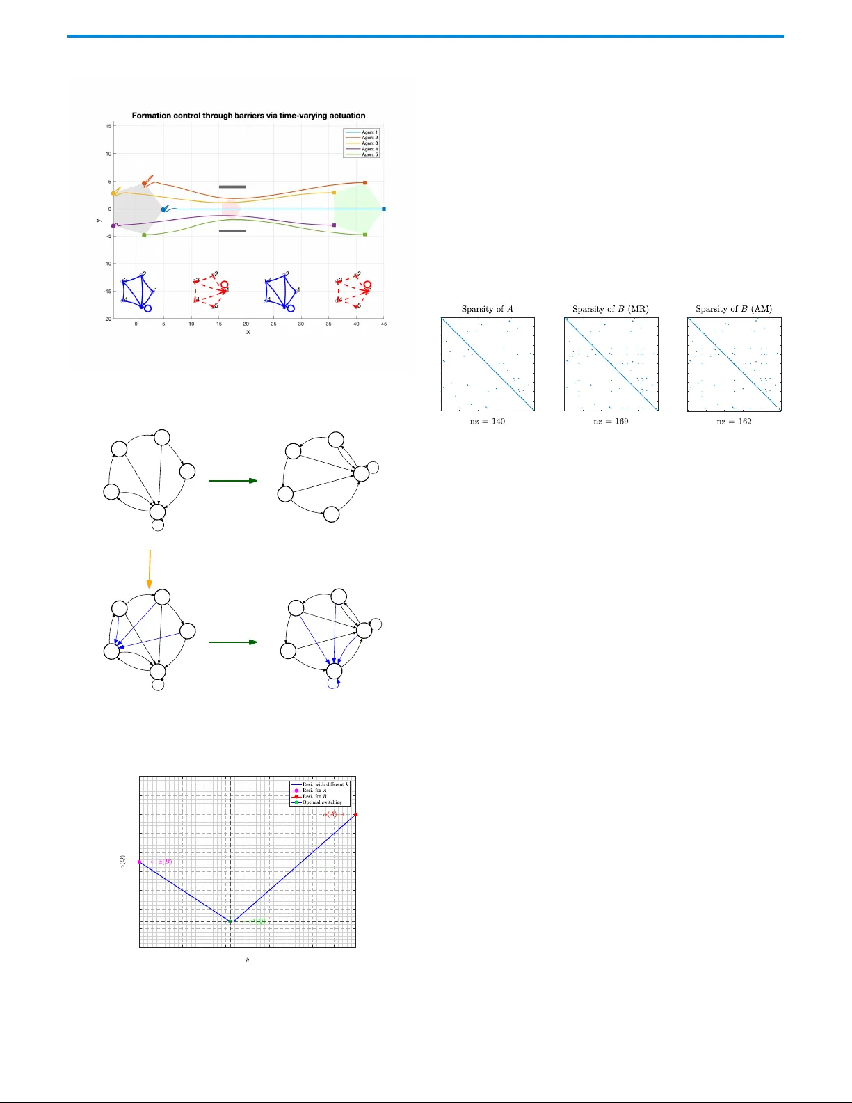
GENERIC COLORIZED JOURNAL, V OL. XX, NO . XX, XXXX 2017 1 Enhancing network resilience through topological s witching F ei Chen, Jorge Cor t ´ es, F ellow , I EEE , and Sonia Mar t ´ ınez, Fello w , IEEE Abstract — This work studies how to pree mptively in- crease t h e resilien ce of a network by means of time-varyin g topologi cal actuation. T o do this, we focus on li near dynam- ical systems that are compatible with a given network, and consid er policies that switch pe riodical ly between the given one an d an alternative , top o logica lly-compatible dyna mics. In par ticula r , we see k to solv e design problems a imed at finding a) the op timal switching schedule between two presele cted topologi es, and b) an optimal topology a nd optimal switching schedule . By imposi n g periodi city , we first provide a metric of resilien ce in terms of the s pectral abscis sa of the averag ed linear time-inv ariant dynamics . By restrictin g our polici es to commutative ne tworks, we then show how the optimal scheduling problem reduces to a con vex o ptimization, providing a bound on the net resilien ce that can be achieve d . After this, we find that the optimal, sparse commutative ne twork to switch with is fully dis connec ted and a llocat e s the spe ctral sum among the node s of the ne t work equa l ly . We then impose addi- tional restricti ons on to pology edge selec tion, which le ads to a biconvex o p timization for which cer tain matrix ra n k conditio ns guide the c hoice of we i ghting parameters to obtain desira ble s olutions . Finally , we p rovide two methods to sol ve this problem efficien tly (based on a McCormick relaxat i on, and alt ernating minimization ) , and il l ustrate the results in simulations . Index T e rms — Ne twork resi lience , time-vary ing actua - tion, op timal s witching, spa rsity-promoting optimizatio n. I . I N T R O D U C T I O N Networked systems find broa d application in div erse do- mains such as rob otics, so c ial network s [ 1], security [ 2], and intelligent transpo r tation systems [3]. While significant progr ess has b e en made in developing their f unction, ne t- worked systems remain highly v u lnerable to various forms of attack s and failures. As the depen d ence o f infr astructure systems on networked systems g rows, so do es the harmful impact o f attack s, with great social an d eco nomic co st. Here, we study how to make networks more resilient to stru ctural attacks, aimed at disrup tin g the top o logy that supports the network operation. I n particular, we are interested in qua n tifying how switching b etween comp lementary meshes can reduce the imp act of a un k nown and fixed top ological Fei Che n is w i th the Depar tment of Aeronautics and Astronautics, Massachusetts Institute of T echnology , Cambrid g e, MA 02139, USA (email: feic@ mit.edu). T his work was conducted w h e n he was at the Univers ity of California, San Diego . Jorge Cor t ´ es and Sonia Mar t´ ınez are with the Depar tment of Mechan- ical and Aerospace Engineering, University of California, San Die g o, CA 92093, USA (e-mail: cor tes@ucsd.edu; soniamd@ucs d.edu). failure. As switching can lead to instability , this requir es the careful design of the time-varying ac tu ation stra tegy to gether with the selection of complemen tary meshes fo r con trol. The resilience of n etworks describ ed by linear time-inv ariant dynamics is often an alyzed throu gh metrics d e r iv ed from the spectr a l an d pseudo -spectral proper ties of the associated matrix. Specifically , the pseudo - spectral ab scissa [4] is a key metric for assessing th e sensitivity of a d ynamical system to perturb ations. Existing algorith ms to co mpute it include the criss-cross algo rithms [5], [6], which rely on the bisection method [7], and [8], [9], which provide fast iterations that exploit the sparse structur e of m atrices. The stability rad ius is a related notio n that aims to capture the smallest pertur bation required to de stab ilize a system. Th e work [1 0] app r oximates the stability radiu s of spa rse m atrices lev eraging [ 8]. In [11 ], the au thors characterize the analogs of these notions for a class of constrained stru c tu red p e r turbation s, pr oposing iterative algorithm s that are capable of tackling networks with hun dreds of n odes. The literatu re on time- varying network systems is mu c h more limited with most of the fo cus on ach ieving stability despite different types of attacks an d under in te r mittent or time-varying co m municatio n s. Some early work includ es [12], [13], on sy stem stabilization unde r Den ial of Service and reply attacks, [14 ] on distributed o ptimization un der adversarial nodes, or [15] on attack d etection and identification. More recently , [16] introd uces a sing le - time-scale distributed state estimation alg orithm under time- varying graphs and worst- case adversar ial attacks, while [17] p roposes a distributed interval estimation algorithm for ar bitrary attack iso la tio n. In contrast, the work [1 8] proposes switching as a defen se mechanism against rational ad versaries with par tial knowledge on an oper ator’ s de cisions. The first co ntribution of this work is an analysis o f how switching between two given topolo g ies can incr ease the resilience of a g iv en network. By prescrib ing periodic chang e s between two linear dy namics, we ease th e time- varying sys- tem analysis to an a veraged linear tim e-inv a r iant coun te r part, which allo ws u s to identify the spectral abscissa o f the latter as the resilience metric of inter est. Th en, we for mulate and solve design problems of in c reased dif ficulty to op tim ize th is metr ic. First, we loo k for an optimal switching schedule between two commutative n etworks, and show how this prob lem reduces to a co n vex optim ization. In p articular, we bo und net resilience using the largest eigenv a lue of each system m atrix together with the eigen value of the other matr ix associated with the 2 GENERIC COLORIZED JOURNA L, VOL. XX, NO. XX, XXXX 2017 same eigen vector . Second , we consider th e join t design of both a co m plementar y network an d the associate d optimal schedu le. This is done by including a sparsity-promoting term in the problem co st that results into a hard op tim ization. I nterest- ingly , we are a b le to show th at the best commutative topology is o ne th at match es a completely disconne c ted network. After this, we further constrain the problem to limit the set edges that can be mo dified. W e find an algebraic rank cond ition that establishes when a com patible commu tativ e network exists and obtain biconv ex prob lem formu lations to so lve the associated problem . Finally , we introd uce two efficient algorithm s (based on McCor mick relax ation and alternating minim ization alg o - rithms) to c o nstruct the complemen tary network, and ev aluate their effectiveness in simulation. I I . P R E L I M I N A R I E S In th is section, we introdu ce n o tations used throug hout the paper, summa rizing main concep ts f rom Floquet theo r y [1 9]. 1) Nota tion : In wh at f ollows, I d denotes the d × d id entity matrix. Given a matrix A = [ a ij ] ∈ R n × n , a ij denotes its i j -th en try , T r( A ) ref ers to its trace, an d vec( A ) ∈ R n 2 is the vecto rized fo rm of A obtaine d b y stacking its columns. By rank( A ) we denote the rank of A , and b y nu llity( A ) the dimen sion of its n ull sp ace. For a vector v = [ v 1 , v 2 , . . . , v n ] T ∈ R n , diag (v) rep resents the diag - onal matr ix with diagon al eq ual to v . Th e span o f A i ∈ R n × n , i ∈ { 1 , . . . , k } , is defined as s pa n { A 1 , A 2 , . . . , A k } = { c 1 A 1 + c 2 A 2 + · · · + c k A k | c 1 , c 2 , . . . , c k ∈ R } . The oper- ation A ⊙ B repre sents the element- wise (Hadam a rd) multipli- cation of matrices A an d B . The Kronecker produ ct o f A an d B is den o ted by A ⊗ B . A row vector of zeros of appro p riate dimensions is represented by 0 ⊤ . The indicator function χ is defined such that χ ( z ) = 1 , if z 6 = 0 , and χ ( z ) = 0 , if z = 0 . W ith this, we define k A k ℓ 0 = P n i,j =1 χ ( a ij ) and, similarly , k A k ℓ 1 = P n i,j =1 | a ij | . The o perator Re maps a matrix or vector to its en try-wise r e al p art. W e deno te b y |I | the cardinality of a set I . By B ǫ := { ∆ ∈ C n × n | k ∆ k F ≤ ǫ } we represent a closed ball centered at 0 with radius ǫ in C n × n , and k · k F denotes the Frob enius n orm. 2) Spe ctral abscissa and worst-case p er tu rbation : Th e spec- tral abscissa of a square matrix A is defined by α ( A ) := max λ ∈ Λ( A ) Re λ, (1) where Λ( A ) is the spectru m (the set of the eigenv alues) of A . Given ǫ > 0 and a closed set H ⊆ C n × n , the structured ǫ -pseudo spectrum of A is Λ ǫ, H ( A ) := { λ ∈ Λ( A + ∆) , ∆ ∈ H ∩ B ǫ } , (2) which represents the union of the spectrum of A + ∆ , for ∆ ∈ H ∩ B ǫ . When H = C n × n , Λ ǫ, H reduces to the usual ǫ - pseudospe c trum [9]. The stru c tured ǫ -pseudo spectral abscissa of A is then expressed as α ǫ, H ( A ) := max λ ∈ Λ ǫ, H ( A ) Re λ = max ∆ ∈H∩ B ǫ α ( A + ∆) . (3) W e call a maximizer ∆ opt of α ǫ, H ( A ) as a worst-case per tur- bation of A of energy ǫ . 3) Flo quet theo ry : Floquet theo ry [ 1 9] provides a mecha - nism to analyze linear time- varying perio d ic systems by m eans of an averaged time-inv ariant cou nterpar t. Briefly , consider ˙ x ( t ) = S ( t ) x ( t ) , x ( t 0 ) = x 0 , (4) where x ( t ) ∈ R n , and S ( t ) ∈ R n × n is piecewise continu ous, bound ed, a n d periodic with p eriod T , i.e., S ( t + T ) = S ( t ) . Floquet theory states that • There exists a no n singular matrix P ( t, t 0 ) with P ( t + T , t 0 ) = P ( t, t 0 ) , an d a con stant matrix Q such that Φ( t, t 0 ) = P ( t, t 0 ) e Q ( t − t 0 ) , where Φ ( t, t 0 ) is th e system state-transition m atrix. • The time-dependen t change of coordinates z ( t ) = P − 1 ( t, t 0 ) x ( t ) transforms (4) in to the following lin e ar time-inv ariant system ˙ z ( t ) = Qz ( t ) , z ( t 0 ) = x 0 . (5) Let R = Φ( t 0 + T , t 0 ) , (6) then Q can be expressed as Q = 1 T ln R. (7) The eigenv a lu es of Q , λ i , i ∈ { 1 , . . . , n } , an d th e eig e nvalues of R , ν i , i ∈ { 1 , . . . , n } , ar e related as f ollows ν i = e λ i T , i ∈ { 1 , . . . , n } . In this way , th e linear time-varying system (4) is exponentially stable if and on ly if R is Schu r or Q is Hurwitz [20]. Therefo re, the stability of (4) can be inferred from th at of (5). I I I . P R O B L E M S T A T E M E N T A N D A P P L I C A T I O N S In this section , we present a f ormal statem ent of the main problem s to be addressed in the r e st of the manuscript. In addition, we in troduce ap p lication scenarios that show th e relev ance of the pro posed pr oblems. A. System descr iption Consider a network r e p resented b y a directed graph or digraph G := ( V , E ) , which con sists of a vertex set V = { 1 , . . . , n } an d an ed ge set E ⊆ V × V . An in-neigh bor of i ∈ V is a vertex j such th at ( i, j ) ∈ E . W e de note the set of in-ne ig hbors of i b y N i . By assigning a weight a ij ∈ R to each edge ( i, j ) ∈ E and a ij = 0 if ( i, j ) / ∈ E , a compatible network dyn amics is described a s the time-inv ariant system ˙ x = Ax, (8) where x ∈ R n are th e stacked states of all agen ts, and A = [ a ij ] ∈ R n × n is the weigh ted adjacency matrix. W e assume th at th e matrix A is Hurwitz, therefo re α ( A ) < 0 . For brevity , we use either A o r the underly ing dig raph G to refer to a network. W e are interested in redu c ing the im pact of a d versarial attac ks on (8) r epresented by multiplicative perturb ations ∆ of the form: ˙ x = ( A + ∆) x. A UTHOR et al. : P REP A R A TION OF P APE R S FOR IEEE TRANSACTIONS AND JOURNALS (FEBRU AR Y 2017) 3 Since the worst-case perturb ation, g iven by (2) and (3), depend s on the network structure, it shou ld be possible to adjust it to e nhance its resilience. In particular, the smaller (i.e., more negative) α ( A ) is, the greater th e resilienc e [11 ]. This function is in versely p ropor tional to what can be inter p reted as a distanc e -to-instab ility m etric, which is our goa l to increase. B . Problem statement T o au gment the resilience of (8), we will en large our system with time-varying actuation, as describe d by ˙ x = S ( t ) x. This time-varying actu a tion will b e lim ited to a few actions as specified by a finite set o f topo logical network chan ges. In par ticular , we are interested in under standing a) wh en it is p ossible to achieve a n et re silien c e -improvement by topolog ical switchin g, and b) how to design such new network topolog y an d switchin g sched ule to realize this benefit. T o state these g oals mo re pr ecisely , con sider two n etworks represented by weigh te d matrices A, B ∈ R n × n and as- sociated digraph s G A := ( V A , E A ) and G B := ( V B , E B ) , respectively . A switched sy stem defined by A, B is g iv en by ˙ x ( t ) = S ( t ) x ( t ) = ( Ax ( t ) , t i, 1 + l T ≤ t < t i, 2 + l T , B x ( t ) , t i, 2 + l T ≤ t < t i +1 , 1 + l T , (9) where i ∈ { 1 , . . . , m } and m represents the occurren ces of A and B during a time p eriod T , and t 1 , 1 = 0 , t m +1 , 1 = T ; l ∈ { 0 , 1 , . . . } . Fu rthermo re, we define ∆ t i, 1 = t i, 2 − t i, 1 (resp. ∆ t i, 2 = t i +1 , 1 − t i, 2 ), i ∈ { 1 , . . . , m } , as the dwell time when A (resp. B ) is active. The resilience of the switched system (9 ) will be charac- terized via the spectral abscissa of an associated dy namical system. In the following, we de n ote this fu nction as α ( S ( t )) . W e now fo rmally state the p roblems co n sidered her e. Problem 1. Giv en two networks A , B defining the switched system (9), quan tif y α ( S ( t )) an d derive an o ptimal switching between A , B such that α ( S ( t )) is m inimized. In other words, solve for the o p timization min ∆ t i, 1 , ∆ t i, 2 α ( S ( t )) s.t. 0 < ∆ t i, 1 < T , 0 < ∆ t i, 2 < T , i ∈ { 1 , . . . , m } , m X i =1 (∆ t i, 1 + ∆ t i, 2 ) = T . (10) • Problem 2. Given a network A , op timize th e structural changes of A to o btain a r esilience-enha n cing comp lementary network B such that α ( S ( t )) < min( α ( A ) , α ( B )) , via time- varying actuation as in (9). • C. Ph y sical application scenarios This section pr esents so m e main applicatio n s o f the resilience-enh ancing topolog y-switching problems introduc e d above, showing how these relate to th e abstracted dy nam- ics (8 ). Sectio n VII will revisit these examples in simulation. 1) Forma tion control : Consider a g roup of agents i ∈ { 1 , . . . , n } , and d ivide the se into sets V g and V l , V g ∪ V l = { 1 , . . . , n } , where V g consists of agen ts with privileged access to global information (e.g. by interacting with a fu sion center). Let K i ∈ R d × d be a local gain matr ix , for i ∈ V , a n d w ij a non-zer o positi ve weigh t for an edge ( i, j ) in the agent- interaction graph G = ( V g ∪ V l , E ) . The associated weigh ted Laplacian matrix L w = [ l ij ] ∈ R n × n , is given by l ij = − w ij ∈ R , if i 6 = j , and l ii = P n k =1 w ik , for i ∈ { 1 , . . . , n } . Let |V g | = n g , |V l | = n l , with n g + n l = n . Den ote by z g ∈ R dn g and z l ∈ R dn l the stacked ag ents’ states in V g and V l , respecti vely . Let the weig hted Laplacian matrix L w be divided into blocks L gg , L gl , L gl , L ll , d escribing the interactions with in an d betwee n the gr oups of ag e nts V g and V l , respectively . Similarly , defin e the block - diagon al gain matrices K g = diag( K i | i ∈ V g ) , and K l = diag( K i | i ∈ V l ) . A g eneralized for m ation-co ntrol dy namics is given as ˙ z g = A g z g + A gl z l + r ⋆ ( t ) , (11) ˙ z l = A l z l + A lg z g , (12) where A g = K g + L gg ⊗ I d , A gl = L gl ⊗ I d , A l = K l + L ll ⊗ I d , and A lg = L lg ⊗ I d . The time-varying m apping r ⋆ : R ≥ 0 → R dn g encodes the inform ation tha t only ag e n ts in V g have ac c ess to . By stacking (1 1) and (12), d efining A in a block-wise mann er via A gg , A gl , A lg , A gg , and setting f ( t ) = [ r ( t ) ⊤ , 0 ⊤ ] ⊤ ∈ R dn , we can rewrite the overall dynamics as ˙ z = Az + f ( t ) . (13) In ord er to wr ite (13) in the form of (8), we perform th e ch ange of variables as x = z − g ( t ) , wh ere g ( t ) satisfies th e differential equation ˙ g ( t ) = Ag ( t ) + f ( t ) , g (0) = 0 , which can be calculated in a distributed way and treated as a r eference signal for z . Then , ( 1 3) is equiv alent to ˙ x = Ax . It is well k nown that it is p ossible to choose the set V g and design limited- agent inter actions to e n sure that A is a Hurwitz matrix [21] . Hence, z will track the refer ence signal g ( t ) . A group of ag e n ts may u tilize this appro ach to adjust the relative fo rmation and move safely throu gh a narr ow cor ridor . Howe ver , a disruptio n in agent in teractions may re su lt into collision. Please refer to Section VI I-.1 fo r mor e infor mation. 2) P ower systems : T h e d y namics of ge n erator buses in power n etworks are governed by the swing equation M ¨ θ + D ˙ θ + Lθ = u , which is obta in ed after th e lineariz a tio n of the nonlinear power flow equations aro und a stationary o perating point [ 15], [17 ] and L is the gene r ator network Lap lac ian obtained after a Kro n reduction [22 ] of the load buses in the network admittance matrix. By neglecting the generato r inertia dynamics, the inertia term can be omitted by setting M = 0 , which yields a first-order network dy namics model [23] that retains the essential interconnectio n topo logy , ˙ θ = − D − 1 Lθ + D − 1 u. A feedback g ain m atrix K can b e desig n ed such that the clo sed-loop dyn amics become ˙ θ = − D − 1 ( L + K ) θ, where the matrix K r e present either local o r wide-area con trol interactions amon g the no des [22] . By pr operly designing K , th e clo sed -loop matrix A = − D − 1 ( L + K ) can be made Hurwitz while remaining sparse. The Laplacian L is fixed and characterizes the physical topology of the power 4 GENERIC COLORIZED JOURNA L, VOL. XX, NO. XX, XXXX 2017 network, wh ereas different design s o f K corr espond to dif - ferent fee dback strategies. Switch in g between such f eedback gains K 1 , K 2 enables chan ges in the contro l in ter connec tio n structure an d th e overall resilience can be enhanced . W e refer the reader to Section VII-.3, where we provide details of such an examp le and evaluate its resilience. I V . O P T I M A L S W I T C H I N G F O R C O M M U T A T I V E N E T W O R K S In this section, we fo c u s o n Pro blem 1 . W e first prop o se a definition of α ( S ( t )) via Floq uet th eory . T hen, we pr esent an algorithm to solve Problem 1. A. Resilience metr ic f or switching systems As S ( t ) is piecewise con tinuous, bo unded and pe r iodic; accordin g to Floquet th eory; cf. Section II-.3 , the time- av eraged tr a je c tories of (9 ) can be capture d by the solution of an associated system coun te r part. Thus, ou r q uantification of α ( S ( t )) will rely on the line ar time-inv ariant system ˙ z ( t ) = Qz ( t ) . (14) From ( 6), w e can comp ute R as R = Φ( T , 0 ) : = m Y i =1 e B ∆ t i, 2 e A ∆ t i, 1 = e B ∆ t m, 2 e A ∆ t m, 1 · · · e B ∆ t 1 , 2 e A ∆ t 1 , 1 , which im plies that Q in (7) can b e ob tained as Q = 1 T ln R = 1 T ln( m Y i =1 e B ∆ t i, 2 e A ∆ t i, 1 ) . (15) It is kn own that the switched system (9 ) is exponen tially stable if and on ly if Q in (14 ) is Hurwitz [20] . Th is n aturally leads to the definitio n α ( S ( t )) := α ( Q ) = max λ ∈ Λ( Q ) Re λ, (16) where Λ( Q ) is the spectru m of Q . W e further in vestigate ( 15) to u nderstand how α ( Q ) rela te s to α ( A ) , α ( B ) . The expre s- sion in (15) can be furth er simplified by assuming that A an d B com mute, as stated in the fo llowing assump tion. Assumption 1 (Commutativity) . The two networks r epr e- sented b y m a trices A and B c o mmute; i.e. AB = B A . • Assumption 2 (Network stab ility) . The two networks rep- r esented by matrices A, B ∈ R n × n ar e Hurwitz; i.e., α ( A ) , α ( B ) < 0 . • Lev eraging Assump tion 1, Q can be simplified to Q = 1 T ln( e B ∆ t 2 + A ∆ t 1 ) , where ∆ t 1 = P m i =1 ∆ t i, 1 , ∆ t 2 = P m i =1 ∆ t i, 2 and ∆ t 1 + ∆ t 2 = T . Let k deno te the time ratio during which A is activ e with in o ne per io d, i.e., k = ∆ t 1 /T , 0 ≤ k ≤ 1 . Th en, B is active within the ratio 1 − k . W e can rewrite Q as Q = 1 T ( B ∆ t 2 + A ∆ t 1 ) = (1 − k ) B + k A. (17) Therefo re, we c an analyze ( 1 6) based o n the network prop er- ties of A, B and the dwe ll-time dec ision variable k . B . Time-var ying actuation to enhance resilience The op tim ization pr o blem (10) can b e n ow refo r mulated as the fo llowing resilien c e-optimal switchin g (ROS) pro blem: (R OS) min k α ( Q ) = α ( k A + (1 − k ) B ) s.t. 0 ≤ k ≤ 1 . T o so lve it, we exploit the fact that commu tativ e matrices are simultaneou sly u pper trian gularizab le [2 4]. Ther efore, A = P − 1 U A P, B = P − 1 U B P, (18) where U A and U B are upper-triangu lar matrices with the diag - onal entries giv en by the eigen v alues of A and B , respectively , and P is f ormed by the common eigenvectors to both m atrices. Note that, if both A and B have distinct eigenv alues, U A and U B will be diago nal matr ices. In wh at follows, we gro up the eigenv alues of A and B in pairs, ( λ i , µ i ) , so that λ i , (resp. µ i ) is an eigenv alue of A (resp. of B ), and b oth share the same eigenv ector . W ithout loss of ge nerality , we assume that ( λ 1 , µ 1 ) (resp. ( λ 2 , µ 2 ) ) is the eigenv alue pair such that α ( A ) = Re λ 1 ≡ α A (resp. α ( B ) = Re µ 2 ≡ α B ). In this way , (1 7) becom es Q = k A + (1 − k ) B = P − 1 ( k U A + (1 − k ) U B ) P. Therefo re, the spectr um o f Q is th e sam e as th e spectrum of k U A + (1 − k ) U B , wh ich, in turn, it also is an upp er triangu lar matrix. Mor e pre c isely , Λ( Q ) = { k λ i + (1 − k ) µ i , | λ i ∈ Λ( A ) , µ i ∈ Λ( B ) } . W ith this, ROS is e q uiv alent to the problem of finding an optimal switching ratio k such th at the real p a r t of the rightmost eig en value of Q is m inimized; or, e q uiv alently , so that the so-called resilience- o ptimal switching rROS problem (rROS ) min k x s.t. 0 ≤ k ≤ 1 , x ≥ k Re λ i + (1 − k ) Re µ i , i ∈ { 1 , . . . , n } , is solved. Den ote b y k ⋆ the optimal k that solves rROS , and by x ⋆ = α ⋆ ( Q ) th e o ptimal value that solves rROS . Next, we look f or co n ditions th a t can ensure α ( S ( t )) < min( α ( A ) , α ( B )) while providing a b ound f or α ⋆ ( Q ) , und e r the fo llowing assump tion. Assumption 3 (Un ique Max ) . There is a uniqu e eigenvalue of A (r esp. B ) tha t atta ins α ( A ) ( r esp. α ( B ) ). Tha t is, |{ i | Re λ i = α ( A ) }| = |{ j | Re µ j = α ( B ) }| = 1 . • Theorem 1 (Bound on switch e d system r esilience) . Let A and B be two n etworks satisfying th e commuta tivity Assumption 1, and which define the corr esponding switched system (9 ) . If Assumption 3 on the u nique max holds, then the r esilience of the switched system, characterized by ( 1 6) , is e n hance d ; i.e. α ⋆ ( Q ) < min( α A , α B ) , if an d only if β B < α A and β A < α B , (19) wher e ( α A , β B ) = (Re λ 1 , Re µ 1 ) and ( β A , α B ) = (Re λ 2 , Re µ 2 ) , respectively . Furthermore , α ⋆ ( Q ) is bo unded A UTHOR et al. : P REP A R A TION OF P APE R S FOR IEEE TRANSACTIONS AND JOURNALS (FEBRU AR Y 2017) 5 by the follo wing ineq uality: max( β A , β B ) < α A + δ A δ A + δ B ( β B − α A ) = α B + δ B δ A + δ B ( β A − α B ) ≤ α ⋆ ( Q ) < min( α A , α B ) , (20) wher e δ A = α A − β A and δ B = α B − β B . Pr oo f. W e first prove the “on ly if” p art (the nece ssary condi- tion); that is, if α ⋆ ( Q ) < min ( α A , α B ) , then c ondition (19) must hold . Acco rding to r R OS , we want to minimize x while satisfying th e con straints x ≥ k Re λ i + (1 − k ) Re µ i , f or all i ∈ { 1 , . . . , n } . Let us de fin e f i ( k ) = k Re λ i + (1 − k ) Re µ i , i ∈ { 1 , . . . , n } . W ithout loss of g enerality , den ote by f 1 ( k ) = k α A + (1 − k ) β B and f 2 ( k ) = k β A + (1 − k ) α B , wh ic h we refer to as “do minant segments”. 1 Note th at, if k ⋆ = 0 , th e o p timal value is x ⋆ = α B , which m e ans that we fix the ne twork to B . While wh en k ⋆ = 1 , the optimal value is x ⋆ = α A , setting the network equ al to A . Both c ases are tr i vial and the resilience does n o t impr ove with respect to th at provid e d by either A or B . The only possible way to improve resilienc e; th at is, α ⋆ ( Q ) < min { α A , α B } , r equires that k ⋆ ∈ (0 , 1) . T o stu dy this ca se, we co nstruct the following optimization p roblem: (A O 1 ) min k x s.t. 0 ≤ k ≤ 1 , x ≥ k α A + (1 − k ) β B , x ≥ k β A + (1 − k ) α B , and let x ⋆ denote its optimal solutio n ( similar ly , let k ⋆ be the correspo n ding optimal k for this pro blem). W e know th a t x ⋆ ≤ x ⋆ , sin ce th e constra in ts of AO 1 form a subset of those of rROS . Th e KKT conditio ns for A O 1 characterize its solu tions and a r e ob tained next. Fir st, d efine L ( k , x, θ 1 , θ 2 , ν 1 , ν 2 ) = x + θ 1 ( k α A + (1 − k ) β B − x ) + θ 2 ( k β A + (1 − k ) α B − x ) − ν 1 k + ν 2 ( k − 1 ) , where θ 1 , θ 2 ≥ 0 are the Lagra n ge mu ltipliers associated with x ≥ f 1 ( k ) and x ≥ f 2 ( k ) ; r espectively , ν 1 , ν 2 ≥ 0 are the Lagrang e mu ltipliers associated with 0 ≤ k ≤ 1 . The KKT condition s f or th e op tim al solution s are as follows: • Stationarity: First, ∂ L ∂ x = 1 − θ ⋆ 1 − θ ⋆ 2 = 0 , which leads to θ ⋆ 1 + θ ⋆ 2 = 1 . Secon d, ∂ L ∂ k = θ ⋆ 1 ( α A − β B ) + θ ⋆ 2 ( β A − α B ) − ν ⋆ 1 + ν ⋆ 2 = 0 . • Primal fe a sib ility: x ⋆ ≥ k ⋆ α A + (1 − k ⋆ ) β B , x ⋆ ≥ k ⋆ β A + (1 − k ⋆ ) α B , 0 ≤ k ⋆ ≤ 1 . • Dual fe a sibility: θ ⋆ 1 , θ ⋆ 2 , ν ⋆ 1 , ν ⋆ 2 ≥ 0 . 1 W e refer to f 1 , f 2 as dominant segments because there are value s of k for which they dominate all others: for k = 1 , we have f 1 (1) = α A ≥ f i (1) for all i , and for k = 0 , f 2 (0) = α B ≥ f i (0) , for all other i . • Complemen tary slackness: θ ⋆ 1 ( k ⋆ α A + (1 − k ⋆ ) β B − x ⋆ ) = 0 , θ ⋆ 2 ( k ⋆ β A + (1 − k ⋆ ) α B − x ⋆ ) = 0 , ν ⋆ 1 · ( − k ⋆ ) = 0 , ν ⋆ 2 · ( k ⋆ − 1) = 0 . Note that, if x ⋆ = α ⋆ ( Q ) < min( α A , α B ) , then x ⋆ < min( α A , α B ) . Th e refore, it must be that 0 < k ⋆ < 1 . This, togeth er with the comp lementary slack n ess, imp lies th at ν ⋆ 1 = ν ⋆ 2 = 0 , which simplifies th e station arity co nditions as θ ⋆ 1 + θ ⋆ 2 = 1 , (21) θ ⋆ 1 ( α A − β B ) + θ ⋆ 2 ( β A − α B ) = 0 . (22) If θ ⋆ 1 = 0 or θ ⋆ 2 = 0 (or equ iv alently , fro m ( 21), if θ ⋆ 2 = 1 o r θ ⋆ 1 = 1 , respec tively), then, from (22 ), we obtain β A = α B or α A = β B ; respecti vely . From th e first two equ ations of Complemen tar y slackn ess, this implies that x ⋆ will either be x ⋆ = α B or x ⋆ = α A ; respectively , an d resilience is n ot improved. The r efore, θ ⋆ 1 , θ ⋆ 2 > 0 mu st hold , which confirm s that the do minant-segmen t constraints are active, x ⋆ = k ⋆ α A + (1 − k ⋆ ) β B = k ⋆ β A + (1 − k ⋆ ) α B . (23) Assume n ow that θ ⋆ 1 , θ ⋆ 2 > 0 a n d consider (22). The latter holds in two possible ca ses. First, suppose that α A − β B = 0 and β A − α B = 0 . From (23 ), it must be that α A = β B = β A = α B . This leads to a co n tradiction with Assump tion 3, on the Uniq u e Max. The seco nd case is α A − β B β A − α B = − θ ⋆ 2 θ ⋆ 1 < 0 . Due to the definition of the spectra l ab scissa (1) and Assumption 3, the cond itions β B > α A and β A > α B cannot both be true, as it lead s to β A > α A , a contrad ic tio n. Con seq uently , ( α A − β B )( β A − α B ) − 1 < 0 only when (19 ) ho lds. The “if” part (the sufficient con dition) fo llows fro m ge o - metric co nsideration s. Since α A > β A and α B > β B , th en f 1 ( k ) (r e sp. f 2 ( k ) ) is inc r easing (r esp. decr e asing) over [0 , 1] . Note th at, under con dition ( 19) and Assump tion 3, th e solu tio n to AO 1 , k ⋆ ∈ (0 , 1 ) an d x ⋆ must b e attain ed at the value o f intersection, x ⋆ = f 1 ( k ⋆ ) = f 2 ( k ⋆ ) (o therwise, x ⋆ is achieved at k ⋆ = 0 or k ⋆ = 1 , wh ich implies α A = β A , o r α B = β B , contradictin g Assump tio n 3). W e th en in vestigate the case when x ≥ f i ( k ) is active, for some i ∈ { 3 , . . . , n } . Consider the segment f ( k ) = α B + k ( α A − α B ) , k ∈ [0 , 1] . Note that it always holds that f ( k ) > f i ( l ) , fo r all l , k ∈ [0 , 1] , an d fo r any f i ( k ) = Re( µ i ) + k (Re( λ i ) − Re( µ i )) , i ∈ { 3 , . . . , n } . Otherwise, and d ue to Assum ption 3, b oth segments intersect at a k ∈ (0 , 1 ) , an d either f i dominates over f on ( k , 1] , or on [0 , k ) . But if the fo r mer, the n α A = f (1) < f i (1) = Re( λ i ) , and, if the latter, then α B = f (0) < f i (0) = Re( µ i ) , a contradictio n. There fore, if a solu tion k ⋆ is attained at an f i , i ∈ { 3 , . . . , n } , we have that either x ⋆ = f i ( k ⋆ ) < α A = f (1) , x ⋆ = f i ( k ⋆ ) < α B = f (0 ) . In other words, x ⋆ = α ⋆ ( Q ) < min { α A , α B } . T o prove the ineq u ality (20), we alread y have that α ⋆ ( Q ) < min( α A , α B ) provided that condition (19 ) is satisfied. W e then solve (23), and obtain x ⋆ as x ⋆ = α A + δ A δ A + δ B ( β B − α A ) = α B + δ B δ A + δ B ( β A − α B ) with δ A = α A − β A and δ B = α B − β B , and th e correspo nding k = δ B δ A + δ B ∈ (0 , 1) . Given that 6 GENERIC COLORIZED JOURNA L, VOL. XX, NO. XX, XXXX 2017 x ⋆ ≤ α ⋆ ( Q ) , the equality and second inequality fr om the left of (20) ho ld . Fur thermor e, α A + δ A δ A + δ B ( β B − α A ) − β B = k ( α A − β B ) > 0 and α B + δ B δ A + δ B ( β A − α B ) − β A = (1 − k )( α B − β A ) > 0 . This establishes the satisf action of (20). W e gener a lize Theorem 1 to the case o f mu ltiple eigenv al- ues, an d the results are summarized in Corollary 1. W e fir st define the index set J as J = { j | ( λ j , µ j ) with Re λ j = α A or Re µ j = α B } i.e. , the pairs o f eigenv alues f o r which either λ j or µ j attain th e spectr al ab scissa value. The dominan t segments are d efined as f j ( k ) = k Re λ j + (1 − k ) Re µ j , j ∈ J , and another a u xiliary optimization pro blem is pro posed: (A O 2 ) min k x s.t. 0 ≤ k ≤ 1 , x ≥ f j ( k ) , j ∈ J . Corollary 1 (Bo u nd on switched system resilien c e, general case) . Let the prer equisites of Theorem 1 h old, except for Assumption 3 . Th en, α ⋆ ( Q ) < min( α A , α B ) if and only if the following con ditions hold : if Re λ i = α A for so me i, the n Re µ i < α A ; (24) if Re µ j = α B for so me j, th en Re λ j < α B . (25) Furthermore , α ⋆ ( Q ) is b ound e d b y the following inequ a lity: x ⋆⋆ ≤ α ⋆ ( Q ) < min ( α A , α B ) , (26) wher e x ⋆⋆ is the op timal value of pr o b lem AO 2 . Pr oo f. The proo f extends the a rgu ments of T h eorem 1. In cases whe r e multip le eigenv alues achieve the spectra l abscissa value, e very pair must satisfy a similar if an d only if con dition as stated in ( 1 9), lea ding to the co nditions ( 24) and (2 5). Moreover , since there are more dominan t se gments serving as constraints in AO 2 compare d to AO 1 , the resultin g lower bound is o b tained by solving AO 2 . Con sequently , the bo und in (26) is a generalizatio n of ( 20). Remark 1 ( Enhanc in g resilience) . T o augme nt r e silien c e throug h tim e -varying a ctuation, the networks A and B n eed to exhibit opposite proper ties that lead to a “mismatch” in their eigenv alues, as ind icated by (19 ), (24), (2 5). Fur thermor e, th e bound s (20) a n d ( 26) are lin ked to the e ig en value pairs tha t determine th e r esilience of each individual network. • Finally , we summar ize in Algor ith m 1 the propo sed ap- proach f or d eriving the op timal switching between A and B . Algorithm 1: OptSwitch — Computation of Opt imal Switc h ing Input: A, B s.t. AB = B A Output: k ⋆ , α ⋆ ( Q ) 1 Upp er trian gularize A, B as (18) 2 Pair the eig e n values ( λ i , µ i ) o f A, B with r espect to the same eigenvector 3 Comp ute th e real part of λ i , µ i 4 Solve the linear p r ogramm ing rROS 5 return k ⋆ , α ⋆ ( Q ) V . N E T W O R K S T R U C T U R A L O P T I M I Z A T I O N U N D E R H O M O G E N E O U S S P A R S I T Y C O N S T R A I N T S In this section , we focus on Problem 2 to optimiz e re- silience from a topo logical-desig n p erspective. In this way , giv en a network A , we aim to find a resilience-en h ancing compleme n tary network, B , which we can use toge th er with an optimal switching strategy as in ( 9) so that α ( S ( t )) < min( α ( A ) , α ( B )) . In doing so, we will consider various optimization formulatio n s. Our first pro blem, ℓ 0 -rec , is the following: ( ℓ 0 -rec) min k,B α ( k A + (1 − k ) B ) + k Γ ⊙ B k ℓ 0 s.t. A B = B A, 0 ≤ k ≤ 1 , T r( B ) = T r( A ) . In ℓ 0 -rec , we o ptimize over B com m utative w ith A , as well as over the switching between A an d B . The ob jectiv e fu nction consists of two parts: The first par t is as in ROS (or rROS ), to o ptimize the topolo gy-switchin g ratio, wh ile the secon d part in volves k · k ℓ 0 , a sparsity-p romotin g pena lty func tion defined on th e Hadamar d prod uct of B with a weigh tin g matrix Γ := [ γ ij ] ∈ R n × n . The con straint AB = B A e nsures commutativity , wh ile the seco nd 0 ≤ k ≤ 1 chara c terizes the acti vation of A within one pe riod. The third con straint T r( B ) = T r( A ) is introdu c ed to ensure th at B maintains a spectral scale that is compar a b le to that of A . The ℓ 0 -norm is co mmonly used to ch aracterize sp arsity . Unfortu n ately , this leads to op timization p roblem s that are nonco nvex and NP-hard. A c o mmon approa c h to ad dress this issue is to replace the ℓ 0 -term k · k ℓ 0 with an ℓ 1 -term, k · k ℓ 1 . The ℓ 1 relaxation r esults in to ( ℓ 1 -rec) min k,B α ( k A + (1 − k ) B ) + k Γ ⊙ B k ℓ 1 s.t. A B = B A, 0 ≤ k ≤ 1 , T r( B ) = T r( A ) . Problems ℓ 1 -rec a n d ℓ 0 -rec a r e in general no t equiv alent, being the first a relaxation o f the secon d. In what fo llows, we chara cterize the algebraic co n ditions on B that en sure it commutes with A . Building upo n th ese proper ties, we can rewrite ℓ 1 -rec and o btain new in sight on its relationship with ℓ 0 -rec . For a giv en A , C ( A ) = { B | AB = B A } denotes the cen tralizer of A [ 2 4]. L et λ A = [ λ 1 , · · · , λ n ] T denote the vector of all eigenv alues of A . Th e V andermon de matrix Λ p formed by λ A is defined as Λ p :=      1 λ 1 λ 2 1 · · · λ n − 1 1 1 λ 2 λ 2 2 · · · λ n − 1 2 . . . . . . . . . . . . . . . 1 λ n λ 2 n · · · λ n − 1 n      . (27) The fo llowing lemma states the a lg ebraic pro p erties of C ( A ) using the powers of A , which fo llows fro m Theo rem 3.2.4 .2 of [24] . He r e, we provid e an alternative pro of to this result via the V andermo nde m atrix, which will be help f ul in the sequel. A UTHOR et al. : P REP A R A TION OF P APE R S FOR IEEE TRANSACTIONS AND JOURNALS (FEBRU AR Y 2017) 7 Lemma 1 (Algeb raic characteriz a tion of a matrix centralizer ) . Suppo se that A ∈ R n × n has distinct eigen values. Th en B ∈ R n × n is commutative with A if and only if B ∈ C ( A ) = span { I , A, A 2 , · · · , A n − 1 } . Pr oo f. The “if ” part f ollows imm e diately: we first write B as a linear comb ination o f the basis matrices, i.e., B = P n − 1 i =0 c i A i = c 0 I + c 1 A · · · + c n − 1 A n − 1 . W e then can verif y that AB = B A = P n − 1 i =0 c i A i +1 , thus B is c o mmutative with A . Th e “o nly if ” part can b e p roved via Theo rem 3.2.4 .2 of [2 4] dir ectly . Instead , we p r ove it by leveraging matrix proper ties to establish the con n ection b e twe en th e A, B spec- tra. Since A, B are commutative, they are simultaneou sly upper-triangu la r izable as A = P − 1 X P , B = P − 1 Y P , where X and Y are the up p er-triangular m atrices with diagon al entries given by th e eigen values of A an d B , r espectiv ely . Furthermo re, X is diago nal, X = dia g( λ 1 , · · · , λ n ) , with the diag onal con ta in ing the distinct eigenv alues of A . Since AB = B A , th en X Y = Y X , which y ields λ i y ij = λ j y ij where Y = ( y ij ) . Due to the fact that A h as distinct eigenv alues, ( λ i − λ j ) y ij = 0 implies y ij = 0 for i 6 = j . Therefo re, Y = diag ( µ 1 , · · · , µ n ) is also diagonal with its eigenv alues in the d iagonal. Note that the statement we aim to prove is in variant under similarity transform a tions P , and thus, w .l.o.g. we can fo cus on d iagonal matric e s. W e have that P n − 1 i =0 c i X i = diag( P n − 1 i =0 c i λ i 1 , · · · , P n − 1 i =0 c i λ i n ) . Ther e fore, we o btain Λ p c = µ B , where Λ p is the V andermon de matrix as in (27 ), c = [ c 0 , c 1 , · · · , c n − 1 ] T , and µ B = [ µ 1 , µ 2 , · · · , µ n ] T . The V ande rmond e matrix Λ p is in vertible since X has distinct eigenv alues [24 ], thus we can always o btain a coefficient vector c tha t is a solution to the previous equ ation. Pre an d post-multip ly ing Λ p c = µ B by P − 1 , P , r e spectiv ely , implies that B = P n − 1 i =0 c i A i , c i ∈ C . Th is allo ws u s to show that c ∈ R n . Specifically , let c i = a i + b i i fo r i ∈ { 0 , 1 , . . . , n − 1 } , where i is the imag inary un it, and a i , b i ∈ R . Then, B =  P n − 1 i =0 a i A i  + i  P n − 1 i =0 b i A i  . Sin c e A, B ∈ R n × n and the set { I , A, A 2 , . . . , A n − 1 } is linearly independen t, it follows that b i = 0 for all i . This completes the p r oof. W e now establish the equivalence be twe e n ℓ 0 -rec , and ℓ 1 -rec , under cer tain cho ice of weightin g parameters. Theorem 2 (Optima of ℓ 0 -rec and ℓ 1 -rec ) . Su ppose γ ij of th e sparsity-pr omo ting weighting matrix, Γ , ar e all equa l; that is, γ ij = γ , which we r efer to as a homogeneous sp arsity constraint. If the o p timal B ⋆ for ℓ 0 -rec (r esp. ℓ 1 -rec ) satisfie s Assumption 2, on network sta bility , then B ⋆ = T r( A ) n I is an optimal solution for both ℓ 0 -rec a nd ℓ 1 -rec . Pr oo f. T o show the result, we first prove that B ⋆ = T r( A ) n I is optimal for th e following optim ization: (A O 3 ) min k,B α ( k A + (1 − k ) B ) s.t. A B = B A, 0 ≤ k ≤ 1 , T r( B ) = T r( A ) . The op timal solution for AO 3 is attained at k ⋆ = 0 , and B ⋆ = T r( A ) n I . T o see this, first no te that B ⋆ ∈ C ( A ) , thu s B A = AB . The third con straint also h olds as T r( B ⋆ ) = T r( T r( A ) n I ) = n T r( A ) n = T r( A ) . The m inimum value of the objective fun ction is given b y α ⋆ ( Q ) = T r( A ) n , which can be shown by contrad iction. Suppo se that α ⋆ ( Q ) < T r( A ) n . Then, the real p arts of the e igenv alues o f Q ar e smaller than T r( A ) n due to th e definition of spectral abscissa, whic h imp lies that T r( Q ) < n T r( A ) n = T r( A ) . Howev er , it must be that T r( Q ) = T r( k A + (1 − k ) B ) = k T r( A ) + (1 − k ) T r( B ) = T r( A ) = T r( B ) , a co ntradiction . Thus, α ⋆ ( Q ) = T r( A ) n is optimal with B ⋆ = T r( A ) n I and k ⋆ = 0 . W e then prove that B ⋆ = T r( A ) n I is also op timal for both ℓ 0 -rec and ℓ 1 -rec when considering the sparsity-p romotin g cost part. For ℓ 0 -rec , we sh ow that k Γ ⊙ B k ℓ 0 is also min- imized with B ⋆ = T r( A ) n I . First, k Γ ⊙ B ⋆ k ℓ 0 = nγ for the chosen B ⋆ . Due to the assump tion that the optima l solution B ⋆ is Hur w itz, we pr ove optima lity by co n tradiction. Supp ose there exists B such that k Γ ⊙ B k ℓ 0 < nγ . This indica tes that B h as fewer than n no nzero en tries, thus B is singular, which leads to a co ntradiction . Ther e fore, B ⋆ = T r( A ) n I is o ptimal for both the re silien c e p art and the sparsity-p romotin g p a rt, which m eans that it is optimal f or ℓ 0 -rec . For ℓ 1 -rec , we also show th a t the ob jectiv e function k Γ ⊙ B k ℓ 1 on sparsity is min imized with B ⋆ = T r( A ) n I . W e can com pute that k Γ ⊙ B ⋆ k ℓ 1 = − γ T r( A ) . Acc o rding to the third constraint of ℓ 1 -rec , we have that k Γ ⊙ B k ℓ 1 ≥ γ P i | b ii | ≥ − γ P i b ii = − γ T r( B ) = − γ T r( A ) . Therefo r e, B ⋆ = T r( A ) n I is optimal for both the resilience p art an d the sparsity-p romotin g part of ℓ 1 -rec , wh ich means that it is optima l for prob lem ℓ 1 -rec . Hen ce, we c onclude that, when γ ij = γ , ∀ i, j in ℓ 0 -rec and ℓ 1 -rec , both prob lems are equiv alent with a solutio n B ⋆ = T r( A ) n I . Theorem 2 provides a sufficient condition under which problem s ℓ 0 -rec and the ℓ 1 -rec are eq uiv alent. However , th e optimal solution B ⋆ = T r( A ) n I plac e s all non -zero entries of B on its diagon al due to the uniform cho ice of γ . In practice, we may b e inter ested in alternative solutions g u ided by add itional design constraints, e.g., restricting the support of B to a subset S of edges that an oper a tor can m odify . T h is solution shou ld also be hard er to gu e ss by an ad versar y . Motiv ated by this, we study th e conve xity o f an associated problem a n d explore how to select the weighting parameters to avoid trivial solutions. V I . N E T W O R K S T RU C T U R A L O P T I M I Z A T I O N U N D E R H E T E R O G E N E O U S S P A R S I T Y C O N S T R A I N T S Based on Lemma 1, we can write B as a linear comb ination B = c 0 I + c 1 A + · · · + c n − 1 A n − 1 or in vectoriz e d form as vec ( B ) = c 0 vec ( I )+ c 1 vec ( A )+ · · · + c n − 1 vec ( A n − 1 ) ∈ R n 2 . Denote A p = [vec ( I ) , · · · , vec ( A n − 1 )] ∈ R n 2 × n , where we form A p by stacking the vectorized basis matrice s as columns, and c = [ c 0 · · · c n − 1 ] T . Then we have th at vec ( B ) = A p c. (28) Note that we vectorize B in order to an alyze its entries in a comp act form , where each entry of B is d e te r mined by 8 GENERIC COLORIZED JOURNA L, VOL. XX, NO. XX, XXXX 2017 the corre sponding e n tries of the powers of A . Consequen tly , each entry of B is cha r acterized by a row of A p throug h the coefficient vector c . Let λ T i denote each row vector of the V andermon de matrix Λ p in (2 7). Th en, the eig en value µ i of B can be derived as µ i = P n − 1 j =0 c j λ j i = λ T i c , while Λ( Q ) = { k λ i + (1 − k ) λ T i c } , i ∈ { 1 , . . . , n } . W ith α ( Q ) deno ting th e real par t of the right- m ost e ig en value of Q as in (16), ℓ 1 -rec is equ iv alent to the f o llowing reform u- lated pr oblem r- ℓ 1 : (r- ℓ 1 ) min k,c (max i Re( k λ i + (1 − k ) λ T i c ) + k W A p c k ℓ 1 ) s.t. 0 ≤ k ≤ 1 , vec ( I ) T A p c = T r( A ) . From ℓ 1 -rec to r- ℓ 1 , we replace B with the vectorized form A p c accord in g to L emma 1, and the coe fficient vector c is the new decision variable in stead . Note that W ∈ R n 2 × n 2 is a diagona l weigh ting matrix tha t introd uces the sparsity penalty for each entry of vec( B ) . W e have that W = diag(vec(Γ)) and k W A p c k ℓ 1 = k vec(Γ ⊙ B ) k ℓ 1 . Th erefore , th e term k W A p c k ℓ 1 is equal to the second term of the o bjective f u nction in ℓ 1 -rec . Next, similar to rROS , we handle the max op erator v ia a linear pro g ram, an d ref ormulate r- ℓ 1 as th e f ollowing equ iv a - lent problem r 2 - ℓ 1 (r 2 - ℓ 1 ) min k,c,x x + k W A p c k ℓ 1 s.t. 0 ≤ k ≤ 1 , x ≥ Re( k λ i + (1 − k ) λ T i c ) , vec ( I ) T A p c = T r( A ) . The following result establishes the c onv exity of th e refo rmu- lated op timization pr oblems r- ℓ 1 , r 2 - ℓ 1 . Lemma 2 (Conve xity o f th e relaxed pro blem) . r- ℓ 1 , r 2 - ℓ 1 ar e biconve x, i.e., r- ℓ 1 , r 2 - ℓ 1 ar e conve x when fixing k or fixing c . Pr oo f. The co n vexity of r- ℓ 1 , r 2 - ℓ 1 is dete r mined b y that o f the function f ( k , c ) = max i Re( k λ i + (1 − k ) λ T i c ) since all the co n straints are linear . W .l.o .g., a ssum e λ i ∈ R , ∀ i . Observe tha t, wh en c is fixed, f ( k , c ) is the com p osition of two conve x fun ctions, thus it is convex. Similarly , f ( k , c ) is also the co m position of two co n vex f unctions in c , when k is fixed. Howe ver , f ( k , c ) is not conve x in the p air ( k , c ) , as it in volves the bilinear p roduct k c . Motiv ated by the ab ove, we propo se two m ethods to solve the p revious p roblem: on e relies o n an alternatin g minimiza- tion m e th od, and the other on a McCorm ick relax ation. 1) Alte r nating min imization : For commutative A, B ∈ R n × n , we h ave A = P − 1 U A P, B = P − 1 U B P according to ( 18). T herefor e, U B = P B P − 1 and we o btain µ i := ( U B ) ii = e ⊤ i U B e i = e ⊤ i ( P B P − 1 ) e i = T r( e ⊤ i P B P − 1 e i ) = T r( P − 1 e i e ⊤ i P B ) = h E ⊤ i , B i F , whe re e i ∈ R n is the i -th standard basis vector , and E i = P − 1 e i e ⊤ i P . Or eq u iv alently , µ i = ( e ⊤ i P ) B ( P − 1 e i ) = u ⊤ i B v i with u ⊤ i := e ⊤ i P, v i := P − 1 e i . Th en, th e optimizatio n problem using alternating min - imization can be refor m ulated as follows: (am- ℓ 1 ) min k,x,B x + k Γ ⊙ B k ℓ 1 s.t. A B = B A, 0 ≤ k ≤ 1 , x ≥ k Re λ i + (1 − k ) Re( h E ⊤ i , B i F ) , T r( B ) = T r( A ) . In order to solve am- ℓ 1 , we generate se veral rand om initializa- tions of k ∈ [0 , 1] . For any fixed k , the sub prob lem in ( B , x ) is convex. Similarly , fo r any fixed B , the subprob lem in ( k , x ) is also c o n vex and can be solved via linear progr a mming. W e alternate between these two steps until conv ergence, i.e., when the relative d ecrease in the obje c ti ve falls belo w a specified tol- erance o r the max im um number o f itera tio ns is reached. Since each block is solved exactly and each sub problem is conve x, the objective fun ction is non increasing acr oss iter ations and the pro cedure co n verges to a coor dinate-wise local minimum (stationary poin t). Am o ng multiple ran dom initializations, we retain th e solution with the best o bjective value. 2) McCor mick rela xation : A McCormick relaxatio n r elaxes r 2 - ℓ 1 as the following c o n vex optimiza tion; namely , cvx- ℓ 1 , where we introduce a bo u nd c i ∈ [ − a, a ] for each c i , i ∈ { 0 , 1 , . . . , n − 1 } with a c onstant a > 0 . In ad dition, λ A = [ λ 1 , · · · , λ n ] T and 1 d e notes the vector of all ones. (cvx- ℓ 1 ) min k,c,x, w x + k W A p c k ℓ 1 s.t. 0 ≤ k ≤ 1 , − a 1 ≤ c ≤ a 1 , − ak 1 ≤ w ≤ ak 1 , c + ( k − 1) a 1 ≤ w ≤ c + (1 − k ) a 1 , 1 x ≥ Re(Λ p ( c − w ) + k λ A ) , vec( I ) T A p c = T r( A ) . Clearly , cvx- ℓ 1 is a conv ex problem , which can be efficiently solved. Althoug h cvx- ℓ 1 is a relaxation of r 2 - ℓ 1 that provides a lower bound of k for r 2 - ℓ 1 due to McCormick r elaxation, we are still able to find a goo d sparse B by choosing a n approp riate weightin g m a trix Γ or W . A M cCormick relax- ation can be p referab le to oth er approach es due to its efficient implementatio n, which builds on previous prob lem structu r e. This relaxation mainly affects the solu tion of k , but we can run Algorith m 1 ag ain to derive the optimal k o n ce the sparse network B is foun d. W e later summ arize this proced u re and approa c h fo r solvin g Pro b lem 2 in Alg orithm 3. As we previously discussed , the choice o f Γ can signifi- cantly af fect the so lu tion of the network optimiza tio n pro blem. This is shown in Theor em 1 for pro blem ℓ 0 -rec , where B ⋆ = T r( A ) n I . However , B = T r( A ) n I m a y be d eemed to be an “easy guess” by an a dversary . Mo tivated b y this, we study here alternative d esigns for the McCormick re lax ation ab ove and h eterogen eous Γ . T o do this, we start by defining what a desired spar sity p a tter ns is, to p r ovide condition s th at en sure the existence of a com patible comm utative n etwork. Definition 1 (Sp a rsity pattern and compatibility) . Consider a n etwork with n nod es, and associate d dyn amics given by A UTHOR et al. : P REP A R A TION OF P APE R S FOR IEEE TRANSACTIONS AND JOURNALS (FEBRU AR Y 2017) 9 A ∈ R n × n . Let S ⊆ { ( i, j ) | 1 ≤ i, j ≤ n } be a set of ed ges. W e say that network B fo llows the desired sparsity p a ttern S if b ij = 0 , ∀ ( i, j ) ∈ S . Further m ore, we say that B is compatib le with A if there exists a nontrivial co efficient vector c 6 = 0 such that B ∈ C ( A ) under th e sparsity patter n S . • W e now in vestigate cond itions on S that can ensur e th at there exists a co mpatible network B with respect to a given A . Accord ing to (2 8), it holds that vec( B ) = A p c , where c is the coefficient vector for B ∈ C ( A ) . Given S , define the ind ex set I 0 ⊆ { 1 , . . . , n 2 } as I 0 = { h | h = ( j − 1) n + i , ( i, j ) ∈ S } . That is, for a B that follows the sparsity patter n of S , th e set I 0 are th e indices where the correspon ding entries of vec( B ) are zero. Using I 0 , d e fine A ( r 0 ) ∈ R | S |× n , wh ich con sists of the rows o f A p indexed by I 0 . T he fo llowing result e stab lishes a conn ection between th e sp a rsity pattern S , A ( r 0 ) , and the existence of compatib le network B . Proposition 1 (Existence of a com patible n e twork) . Consider a network A with n nod es, an d th e desir ed sparsity pa ttern S with | S | ≥ n for B . Then , there exists a network B that is compa tible with A u nder sparsity pattern S if an d o nly if A ( r 0 ) is rank deficient. Pr oo f. The existence of B that is com patible with A depend s on whe th er we find a n ontrivial co efficient vecto r c 6 = 0 that results into B ∈ C ( A ) und er the sparsity pa ttern S . Acco rding to Definition 1, it r equires that b ij = 0 , ∀ ( i, j ) ∈ S , which specifies that the co rrespon ding en tries of vec( B ) must b e zero b y imposing the cond ition A ( r 0 ) c = 0 . Th erefor e , this is equivalent to findin g c o nditions on A ( r 0 ) such that the equation A ( r 0 ) c = 0 ha s no n-trivial solution s; i.e., c 6 = 0 . (Necessity:) If a compatible B exists, th en A ( r 0 ) c = 0 for a non trivial c . Based on ra n k–nu llity theorem , we have tha t rank( A ( r 0 ) ) + nullit y ( A ( r 0 ) ) = n . Since A ( r 0 ) ∈ R | S |× n with | S | ≥ n , and nullit y( A ( r 0 ) ) ≥ 1 for a non-tr ivial c , we h ave that rank( A ( r 0 ) ) ≤ n − 1 , which leads to that A ( r 0 ) is r ank deficien t. (Su fficiency:) If A ( r 0 ) is r ank deficien t, then rank( A ( r 0 ) ) < n . The r efore, nullit y ( A ( r 0 ) ) ≥ 1 and we know that a nontr i vial c exists such that A ( r 0 ) c = 0 , which implies that b ij = 0 , ∀ ( i, j ) ∈ S . Further more, by constructio n using the non -trivial co efficient vector c , we obtain that vec( B ) = A p c with B ∈ C ( A ) . T herefor e, we conclude that ther e exists a network B that is compa tib le with A und er spa r sity pattern S , w h ich co mpletes th e proo f. Giv en an initially sparse n etwork A , a de sig ner would require a coun terpart B tha t is sparse as well. Th us, in what follows we fo c us o n the case | S | ≥ n in Pro position 1, meaning that B should hav e at least n zero entries to ensur e ma x imal sparsity . In this scenario, A ( r 0 ) is either a square or a tall matrix. T o obtain a sparse and effectiv e B , a natural appr oach is to select as many rows of A p as possible, i. e ., maximize |I 0 | while ensur ing that A ( r 0 ) remains rank -deficient. The pro blem of selecting the maximal nu mber of rows from A p to form a rank-d eficient ma tr ix A ( r 0 ) is in gener al NP-hard , due to the combinato rial natu re of row selection. In the following, we propo se an iterative algo r ithm as shown in Algo rithm 2 to find a sparsity p attern S such th a t | S | is as large as possible, giv en that there exists a network B compatib le with A . Algorithm 2: SCNet — S par sity Pattern Con struction for C o mpatible Net work s Input: A with n nodes Output: S 1 Comp ute the basis for the centr alizer of A as I , A, A 2 , · · · , A n − 1 2 V ectorize I , A, A 2 , · · · , A n − 1 and d erive A p = [vec( I ) · · · vec( A n − 1 )] 3 In itialize: set i = 0 , I i = I 0 ⊆ { 1 , . . . , n 2 } with |I 0 | = n . 4 Comp ute A (0) ( r 0 ) from rows o f A p indexed by I 0 5 while ( A (0) ( r 0 ) is full ra n k) do 6 Update I 0 by ch anging the index 7 Compute A (0) ( r 0 ) from updated I 0 8 end while 9 while ( A ( i ) ( r 0 ) is rank deficien t) do 10 Incremen t i 11 repeat 12 Select r ow in dex j n ot in I i 13 Update I i +1 = I i ∪ { j } 14 Compute A ( i +1) ( r 0 ) based o n index set I i +1 15 if ( A ( i +1) ( r 0 ) is rank deficien t) then 16 Update I i = I i +1 17 break 18 until ( A ( i +1) ( r 0 ) is ran k d e ficient) 19 if ( A ( i +1) ( r 0 ) is full ra n k) then 20 break 21 end while 22 Derive S based o n the index set I i 23 return S In Algo rithm 2, we initialize A (0) ( r 0 ) as a square matrix, whe re | S | = n an d n entries of th e network B are requ ir ed to b e zero. W e then iteratively add r ows to A (0) ( r 0 ) while e n suring that A ( i ) ( r 0 ) remains ra n k deficient. This a pproach allows the resulting network B to b e as sparse as p ossible. The con struction o f S , such th at ther e exists a network B compatible with A , is imp ortant because it provid es guidan ce on h ow to select the weigh ting param eters γ ij in Γ , e nabling the optimization problem cvx- ℓ 1 to yield a sparse network B . Sp ecifically , let γ and γ be p ositiv e weig hting p arameters, where γ is sign ificantly smaller than γ , i. e . , γ ≪ γ . Based on the resultin g sparsity pattern S ob tained from A lg orithm 2, we set γ ij = γ if ( i, j ) ∈ S , and γ ij = γ if ( i, j ) / ∈ S . W ith a method for s electing Γ , we are now p repared to propo se an appr oach using the McCormick relax ation to solve Problem 2 , as sum marized in Algor ithm 3. The pro cedure begins by c onstructing the basis fo r th e ce n tralizer of A and the V andermon de m atrix Λ p as in (27 ). Next, Algor ithm 2 is run to find S , which is then employed to select the weig h ting parameters. The matrix B is then obtained solving cvx- ℓ 1 . Finally , Algo rithm 1 is run to determine k ⋆ and α ⋆ ( Q ) . 10 GENERIC COLORIZED JOURNA L, VOL. XX, NO. XX, XXXX 2017 Algorithm 3: SPNO pt — S parsity- P ro moting N etwork Opt imization Input: A with n nodes, positive constants a, γ , γ Output: B s.t. AB = B A , k ⋆ , α ⋆ ( Q ) 1 Comp ute th e basis for th e centr alizer o f A as I , A, A 2 , · · · , A n − 1 2 V ectorize I , A, A 2 , · · · , A n − 1 and d erive A p = [vec( I ) · · · vec( A n − 1 )] 3 Comp ute T r( A ) and the eigenv alues of A a s λ i , i ∈ { 1 , . . . , n } 4 Derive λ A = [ λ 1 , · · · , λ n ] T and th e V ander monde matrix Λ p as in (2 7) 5 Run Algorith m 2 for the desired sparsity pattern S 6 Select the weighting matrix Γ = [ γ ij ] with γ ij = γ if ( i, j ) ∈ S , and γ ij = γ if ( i, j ) / ∈ S 7 Comp ute th e diago n al weighting m atrix W = diag (vec (Γ)) 8 Solve the convex optimization cv x- ℓ 1 to obtain B 9 Run Algorith m 1 for the accu r ate k ⋆ , α ⋆ ( Q ) 10 return k ⋆ , α ⋆ ( Q ) , B V I I . S I M U L A T I O N S A N D E X A M P L E S Here, we pr esent simulations on th e scena rios discussed in Section II I-C to validate ou r previous results. W e b egin with a small-scale network and a f ormation contro l p roblem, followed by larger-scale numer ical and power grid network examples. 1) Resili ent formatio n con trol : W e consider a te a m of five agents in R 2 maintaining a pentago nal form ation as they trav erse a con fined barr ier region. W e a d opt an initial 5-n o de topolog y p resented in [11] as a toy illustration. The grap h correspo n ding to th is top ology A is shown in Fig. 2 with A =       0 1 0 0 0 0 0 1 0 0 0 0 0 1 0 0 0 0 0 1 − 150 − 260 − 187 − 69 − 13       . This matrix is giv en as A = − ( L w + K ) , w h ere L w is the weighted Laplacian and K is a gain m atrix that mo difies th e entries of L w . The matr ix is then employed as in Section III -C in a Kronecker p roduct to obtain the correspondin g 2D vehicle formation system. T he for mation is driven b y a time- varying referenc e signal g ( t ) that smo othly contracts the pen tagon to fit throug h the narrow barrier region and then re-expands it. Here, note that all 5 agents are leader s that h av e the access to th is signal. The closed- form expression of g ( t ) is giv en as follows: Let θ i = 2 π ( i − 1) / 5 , i ∈ { 1 , . . . , 5 } . Th e total maneu ver time T = 40 is d ivided into two phases of duratio ns T 1 = 1 7 . 144 and T 2 = T − T 1 = 22 . 856 . For each ag ent i , the ref erence g i ( t ) is g i ( t ) =     t +(1 − φ 1 ( t )) r w cos θ i + φ 1 ( t ) r n cos θ i (1 − φ 1 ( t )) r w sin θ i + φ 1 ( t ) r n sin θ i  , 0 ≤ t ≤ T 1 ,  t +(1 − φ 2 ( τ )) r n cos θ i + φ 2 ( τ ) r w cos θ i (1 − φ 2 ( τ )) r n sin θ i + φ 2 ( τ ) r w sin θ i  , T 1 ≤ t ≤ T , where τ = t − T 1 , r n = 2 , r w = 5 an d φ 1 = 0 . 5(1 − cos( π t/T 1 )) , φ 2 = 0 . 5 (1 − co s ( π ( t − T 1 ) /T 2 )) . Stackin g these 2 -dimensional vectors gives th e full g ( t ) ∈ R 10 . Th e bar rier may represent a region where an ad versar y is present, and the goal is to find a complemen tary top ology B and an op timal topolog ical switching that can be used a lo ng entire path of the formation to incr e ase its resilience. The eigen values o f A are − 2 ± i , 3 , − 3 ± i , th us α ( A ) = − 2 . W e run Algo rithm 3 to ob tain a desired commu tativ e n etwork B to enh ance resilience by switching between A and B . As an intermediate step of Alg orithm 3, we execute Algorithm 2 to obtain a sparsity p attern S s uch that a compatible network B exists. T o do th is, we in itialize A (0) ( r 0 ) accordin g to the sparsity pattern S 0 = { (2 , 4) , (2 , 2) , (3 , 3) , (4 , 4) , (5 , 5) } , and rank ( A (0) ( r 0 ) ) = 4 < 5 . The resultin g sparsity pattern S , obtained v ia Algo r ithm 2, is S = { (2 , 2) , (2 , 3) , (2 , 4 ) , (2 , 5) , (3 , 1) , (3 , 3) , (3 , 4) , (3 , 5) , (4 , 1) , (4 , 2) , (4 , 4 ) , (4 , 5) , (5 , 1) , (5 , 2) , (5 , 3) , (5 , 5) } , with | S | = 16 an d th e associated ra nk ( A ( r 0 ) ) = 4 . Based on this, we choose a weigh tin g matrix Γ = [ γ ij ] , wher e γ ij = γ = 10 0 if ( i, j ) ∈ S , and γ ij = γ = 1 if ( i, j ) / ∈ S . Next, via Algorithm 3 we solve th e o ptimization problem cvx- ℓ 1 to obtain the desired network B . The r e sulting g raph is shown as B in Fig. 2 with B =       − 13 − 9 . 35 − 3 . 45 − 0 . 65 − 0 . 05 7 . 5 0 0 0 0 0 7 . 5 0 0 0 0 0 7 . 5 0 0 0 0 0 7 . 5 0       , and α ( B ) = − 2 . 25 . Since the McCormick re laxation affects the solu tion of k , we apply Algor ithm 1 to derive the optimal k ⋆ and the resilience α ⋆ ( Q ) of the switched system under the optimal ratio k ⋆ . T he resulting values ar e k ⋆ = 0 . 42 86 and α ⋆ ( Q ) = − 2 . 5714 < min ( α ( A ) , α ( B )) . Th ese r e su lts indicate that, fo r this multi-agen t formation contro l scenario trav ersing a n arrow barrier region, maintainin g topology A f or a ratio k ⋆ of e ach perio d and topolog y B for the comp lemen- tary ratio 1 − k ⋆ effecti vely enh ances the system’ s resilience via network switchin g. Fig. 1 shows the agents’ traje c tories over a 40s perio d , during which we switch betwe e n to pologies A and B twice: to p ology A is held for k ⋆ of the period (i.e. 17 . 144 s ) and top ology B for 1 − k ⋆ (i.e. 2 2 . 856 s ). W e also plot the resilience of the switched system b etween A and B for different values of the ratio k , as shown in Fig. 3, wh ich shows tha t α ( Q ) is op timal at k ⋆ . W e then add 3 edg e s to n ode 4 with weight a 41 = a 42 = a 43 = 1 . This modifies the network to A ′ as shown in Fig. 2. W e app ly Algorithm 3 to d eriv e the correspo nding compleme n tary network, en suring that resilience is impr oved throug h the time- varying actuatio n strategy . The top ology of the updated network is rep resented as B ′ , where the newly added edges, compared to B , include four edges, one of wh ic h is a self-loop at node 5 . W e com pute α ( A ′ ) = − 1 . 154 2 and α ( B ′ ) = − 1 . 32 17 . The optimal switching ratio k ⋆ and the resilience α ⋆ ( Q ′ ) of th e switching system under the optima l ratio k ⋆ are derived as k ⋆ = 0 . 180 9 an d α ⋆ ( Q ′ ) = − 1 . 9133 8 , which is less than min( α ( A ′ ) , α ( B ′ )) . A UTHOR et al. : P REP A R A TION OF P APE R S FOR IEEE TRANSACTIONS AND JOURNALS (FEBRU AR Y 2017) 11 Fig. 1. Formation control to pass a narrow barr ier region via time- v ar ying actuation. 1 2 3 4 5 1 2 3 4 5 5 4 3 2 1 A B A ′ B ′ Algorithm 3 Algorithm 3 A dd 3 e dges 5 4 3 2 1 Fig. 2. The given network topologi es (left) and the commutativ e networks obtained (right) via Algorithm 3. 0 0.1 0.2 0.3 0.4 0.5 0.6 0.7 0.8 0.9 1 -2.7 -2.6 -2.5 -2.4 -2.3 -2.2 -2.1 -2 -1.9 -1.8 Rightmost eigenvalue of Q with respect to k Fig. 3 . Resilience of the switched system for different k . 2) High -dimensio nal numerical example : W e presen t a nu- merical simula tio n of a 100 -nod e network to test our algo- rithms over lar ger networks. The dyn amics are represented by a spar se matrix A ∈ R 100 × 100 whose spar sity pattern is shown in Fig. 4 . As α ( A ) = − 0 . 6 091 , o ur goal is to de riv e a compleme n tary n etwork, B , which can im prove the resilience of the switched system. In high-dimen sional cases such as this, computin g th e p owers of A i for la rge i become s impractical. This p roblem can be av oided by focusing o n a su bset o f the centralizer of A to c onstruct th e commu tativ e network B . Another op tion is to resort to th e alternatin g minimization method, w h ich d oes no t inv olve ma tr ix powers. 0 20 40 60 80 100 0 10 20 30 40 50 60 70 80 90 100 0 20 40 60 80 100 0 10 20 30 40 50 60 70 80 90 100 0 20 40 60 80 100 0 10 20 30 40 50 60 70 80 90 100 Fig. 4. Sparsity patt er ns of the given n e twork A (left, with 140 nonzero entries), the resilience-enhancing complementar y network B using McCormick relaxation (middle, with 169 nonzero entri es), and the resilience-enhancing complementar y n e twork B using alter nating minimization (r ight, with 162 nonzero entr ies). The given network example h as 140 n onzero entries, thus we explore these o ptions. Sp ecifically , for the McCorm ick relaxation metho d, we first comp ute powers of A up to or der 12 to construct B via Algo rithm 3. T he sparsity pattern o f B der iv ed using the McCormick relaxation thr ough Algo - rithm 3 is sh own in the middle of Fig. 4. The resilience of network B is derived as α ( B ) = − 0 . 328 2 , while the resilience of the switched system unde r optimal switching is α ⋆ ( Q ) = − 0 . 8831 , with th e co rrespon ding optimal r atio of k ⋆ = 0 . 3 226 . Furth ermore , the sparsity pattern of B derived using alternating minim ization v ia the prob lem am- ℓ 1 is shown on the right of Fig. 4. The correspon ding resilience is α ( B ) = 0 , while th e resilience of the switched system under op timal switchin g is α ⋆ ( Q ) = − 1 . 245 7 , with the correspo n ding o ptimal r atio of k ⋆ = 0 . 5 4 72 . Thus, we co nclude that the resilience o f th is example can be enh anced by switching between A and B ; a n d that the best approa c h is given by th e alternating minimization m ethod. 3) Resili ent power network : W e con sid e r the IEEE 1 18-bus system with n = 54 gen erators. The power network data is obtained from the M A T P O W E R p a c kage [25]. The ph ysical coupling is de scribed by th e ge nerator n etwork L aplacian L ∈ R 54 × 54 , whose given phy sical top ology is shown in the first subp lot (in blu e) of Fig. 5 . W ithout lo ss of generality , we set the damp ing ma trix to the identity , D = I n . W e start fr om a d esigned feed back design K 1 , wh ose topo logy is s hown in the thir d su bplot o f Fig . 5 . Th e c o rrespon ding closed-loo p matrix is A = − ( L + K 1 ) , which is both Hurwitz and sparse with α ( A ) = − 0 . 5 . T h e spar sity pattern of A is depicted in the second subplot of Fig. 5. W e then a p ply the alternating minimizatio n p rocedu re to enhan ce re silience since 12 GENERIC COLORIZED JOURNA L, VOL. XX, NO. XX, XXXX 2017 0 5 10 15 20 25 30 35 40 45 50 55 0 5 10 15 20 25 30 35 40 45 50 55 0 5 10 15 20 25 30 35 40 45 50 55 0 5 10 15 20 25 30 35 40 45 50 55 0 5 10 15 20 25 30 35 40 45 50 55 0 5 10 15 20 25 30 35 40 45 50 55 0 5 10 15 20 25 30 35 40 45 50 55 0 5 10 15 20 25 30 35 40 45 50 55 0 5 10 15 20 25 30 35 40 45 50 55 0 5 10 15 20 25 30 35 40 45 50 55 Fig. 5. Sparsity patterns and f eedback topologies f or the IEEE 118-b us system with 54 gener ators. The first subplot (in blue) shows the ph ysical network Laplacian L . The second and f our th subplots (in red) depict the sparsity of the closed-loop matri ces A = − ( L + K 1 ) and B = − ( L + K 2 ) , respectiv ely . The third and fifth subplots (in black) show the corresponding feedbac k topologies K 1 and K 2 . it is more suitab le for high-dimension al cases, as sh own in the pr evious nu merical example. The sparsity p attern of the resulting resilience-enh ancing complementary network B is shown in th e fo urth sub plot of Fig. 5, with α ( B ) = − 4 . 065 7 . The cor respond ing f eedback gain is K 2 = − ( L + B ) , and its top ology is illustrated in th e fifth subplot of Fig . 5. The resilience of the switched system (via different g ain matrices K 1 , K 2 ) u nder optim al switching is α ⋆ ( Q ) = − 3 0 . 307 , with the correspond ing o ptimal ratio o f k ⋆ = 0 . 097 5 . Ther e fore, we can co nclude that the r esilience is g reatly improved throug h the switching between the gains K 1 and K 2 . V I I I . C O N C L U S I O N S In th is pap e r , we study how network resilience can be increased via time-varying actuation by switching b etween pairs of network structures. By p rescribing perio dic switch es, we q uantify resilienc e in term s of the co rrespond ing a ver - aged linear tim e-in variant cou nterpart. Then, we stud y design problem s associated with the optimiza tion o f a) a switchin g schedule between two g iv en topolo gies, and b ) the design o f a compatible topolog y and a switching schedu le to improve the resilience of a giv en network. Futu r e work in cludes the study of resilience for n on-com mutative n etworks a nd expan d ing this design app roach to enhan ce r esilience o f nonlin ear networked systems. R E F E R E N C E S [1] M. Gatti, P . Ca v alin, S. B. Neto, C. Pinhanez , C. dos Santos, D. Gri bel, and A. P . Appel, “Large -scale multi-agent-ba sed m odeling and simu- latio n of microblogging-ba sed online social network, ” in Internationa l W orkshop on Multi-Ag ent Systems and A gent -Based Simulation , Saint Paul , MN, USA, 2013, pp. 17–33. [2] V . Gorodet ski and I. Kote nko, “The multi-agen t systems for com- puter network security assurance: Framewor ks and case studies, ” in IEEE Internatio nal Confere nce on Artificial Intellig ence Systems , Di- vnomorskoe , Russia, 2002, pp. 297–302. [3] B. Burmeiste r , A. Haddadi, and G. Matylis, “ Applicatio n of multi-age nt systems in traf fic and transportat ion, ” IE E Proc eedings-Sof twar e , vol. 144, no. 1, pp. 51–60, 1997. [4] L. N. Trefeth en, Spectra and Pseudospectr a: The Behavior of Nonnor- mal Matrices and Operato rs . Princet on Uni versit y Press, 2020. [5] D. Lu and B. V andere yck en, “Criss-cro ss type algorithms for computing the real pseudospectral abscissa, ” SIAM Journal on Matrix Analysis and Applicat ions , vol. 38, no. 3, pp. 891–923, 2017. [6] J. V . Burke, A. S. Lewis, and M. L . Overton, “Robust stability and a criss-cross algorithm for pseudospect ra, ” IMA J ournal of Numerica l Analysis , vol. 23, no. 3, pp. 359–375, 2003. [7] R. Byers, “ A bisection method for m easuring the distance of a stable matrix to the unstable matrices, ” SIAM Journal on Scientific and Statist ical Computing , vol. 9, no. 5, pp. 875–881, 1988. [8] M. W . Rostami, “Ne w algorithms for computing the real structured pseudospec tral abscissa and the real stability radius of large and sparse matrice s, ” SIAM Journal on Scienti fic Computing , vol. 37, no. 5, pp. S447–S471, 2015. [9] N. Gugliel mi and M. L. Overto n, “Fast algorithms for the approximati on of the pseudospectr al abscissa and pseudospectral radius of a matrix, ” SIAM Journal on Matrix Analysis and Applications , vol. 32, no. 4, pp. 1166–1192, 2011. [10] N. Guglielmi, “On t he method by Rostami for computing t he real stabili ty radius of large and sparse matrices, ” SIAM Journal on Scientific Computing , vol. 38, no. 3, pp. A1662–A1681, 2016. [11] S. Liu, S. Mart ´ ınez, and J. Cort ´ es, “Iterati ve algorithms for assessing netw ork resilie nce against structured perturbati ons, ” IEEE T ransact ions on Contr ol of Network Systems , vol. 9, no. 4, pp. 1816–1827 , 2022. [12] H. S. Foroush and S. Mart´ ınez, “On triggeri ng control of single-input linea r systems under pulse-width modulated DoS jamming attac ks, ” SIAM Journa l on Contr ol and O ptimization , vol. 54, no. 6, pp. 3084– 3105, 2016. [13] M. Zhu and S. Mart´ ınez, “On distribute d constrai ned formation control in operator-v ehic le adversari al netw orks, ” Automatica , vol. 49, no. 12, pp. 3571–3582, 2013. [14] S. Sundaram and B. Gharesifa rd, “Dist ribut ed optimiz ation unde r adver- sarial nodes, ” IEE E T ransact ions on Automatic Contr ol , vol. 64, no. 3, pp. 1063–1076, 2018. [15] F . Pasqual etti, F . D ¨ orfler , and F . Bullo, “ Attack detect ion and identi- fication in cyber -physica l systems, ” IEEE T ransact ions on Automati c Contr ol , vol. 58, no. 11, pp. 2715–2729, 2013. [16] A. Mitra, J . A. Ric hards, S. Bagchi, and S. Sundaram, “Distribute d state estimati on over time-v aryin g graphs: Exploiting the age-of-informat ion, ” IEEE T ransac tions on Automatic Contr ol , vol. 67, no. 12, pp. 6349– 6365, 2021. [17] M. Khajeneja d, S. Brown, and S. Mart ´ ınez, “Distribut ed resilie nt interv al observe r synthesis for nonlinear discrete-t ime systems, ” IEEE T ransac- tions on Automatic Contr ol , vol. 70, no. 10, pp. 6656–6671, 2025. [18] S. Liu, S. Mart´ ınez, and J. Cort ´ es, “Stabiliza tion of linear cyber -physical systems against attac ks via switching defense , ” IEE E T ransactions on Automat ic Contr ol , vol. 68, no. 12, pp. 7326–7341, 2023. [19] G. Floquet, “Sur les ´ equations dif f ´ erentiel les lin´ eaires ` a coef ficien ts p ´ eriodique s, ” Annales scientifique s de l’ ´ Ecole Normale Sup ´ erieur e , vol. 12, pp. 47–88, 1883. [20] C. G ¨ okc ¸ ek, “Stability analysis of periodi cally switche d linea r systems using Floquet theory , ” Mathemat ical Pro blems in Engineeri ng , vol. 2004, no. 1, pp. 1–10, 2004. [21] J. Hu and G. Feng, “Distrib uted tracki ng control of leade r–foll owe r multi-ag ent systems under noisy measurement, ” Automati ca , vol. 46, no. 8, pp. 1382–1387, 2010. [22] F . D ¨ orfler , M. R. Jov anovi´ c, M. Chertko v , and F . Bullo, “Sparsity- promoting optimal wide-are a control of po wer netw orks, ” IE EE T ran s- actions on P ower Systems , vol. 29, no. 5, pp. 2281–2291, 2014. [23] X. Wu and M. R. Jov anovi´ c, “Sparsit y-promoting optimal control of consensus and synchroniza tion networ ks, ” in American Cont r ol Confer - ence , Portland, OR, USA, 2014, pp. 2936–2941. [24] R. A. Horn and C. R. Johnson, Matrix Analysis , 2nd ed. Cambridge Uni versi ty Press, 2012. [25] R. D. Zimmerman, C. E. Murillo-S ´ anchez, and R. J. Thomas, “MA T - POWER: Steady-state operations, plannin g, and analysis tools for po wer systems research and education, ” IE E E T ransact ions on P ower Systems , vol. 26, no. 1, pp. 12–19, 2010.