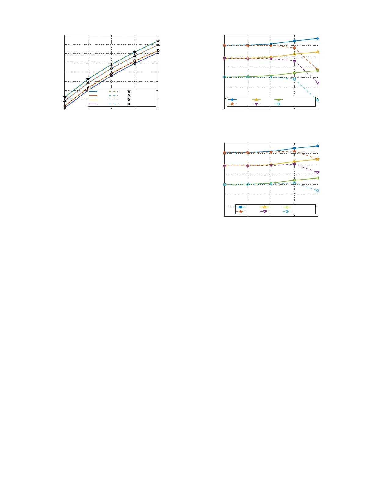
Physics-Compliant Modeling and Optimization of MIMO Systems Aided by Microwave Linear Analog Computers

1 Physics-Compliant Modeling and Optimization of MIMO Systems Aided by Micro wa v e Linear Analog Computers Matteo Nerini, Member , IEEE , Bruno Clerckx, F ellow , IEEE Abstract —Microwa ve linear analog computer (MiLA C) has emerged as a promising architecture f or implementing linear multiple-input multiple-output (MIMO) processing in the analog domain, with radio frequency (RF) signals. Existing studies on MiLA C-aided communications r ely on idealized channel models and neglect antenna mutual coupling. Howev er , since MiLA C performs processing at RF, mutual coupling becomes critical and alters the implemented operation, not only the channel characteristics. In this paper , we develop a physics-compliant model for MiLA C-aided MIMO systems accounting for mutual coupling with multiport network theory . W e derive end-to-end system models for scenarios with MiLA Cs at the transmitter , the recei ver , or both, sho wing how mutual coupling impacts the linear transformation implemented by the MiLACs. Fur - thermore, we f ormulate and solve a mutual coupling aware MiLA C optimization problem, deriving a closed-f orm globally optimal solution that maximizes the received signal power . W e establish the fundamental performance limits of MiLA C with mutual coupling, and deriv e three analytical results. First, mutual coupling is beneficial in MiLA C-aided systems, on average. Second, with mutual coupling, MiLA C performs as digital architectur es equipped with a matching network, while having fewer RF chains. Third, with mutual coupling, MiLA C always outperforms digital architectures with no matching network. Numerical simulations confirm our theoretical findings. Index T erms —Beamforming, gigantic multiple-input multiple- output (MIMO), microwa ve linear analog computer (MiLA C), mutual coupling I . I N T R O D U C T I O N The unprecedented growth of mobile data traf fic and the re- quirements anticipated for sixth-generation (6G) wireless net- works demand transformative shifts in wireless system design [1]. Among the key technologies enabling these capabilities, gigantic MIMO has emerged, exploiting lar ge antenna arrays to increase spectral efficienc y and spatial multiplexing gains [2]. Whereas fifth-generation (5G) systems employ massive MIMO arrays with tens of antennas, 6G visions push to ward gigantic MIMO, in volving hundreds or even thousands of antennas [3]. Ho we ver , scaling con ventional digital MIMO architectures to such dimensions introduces prohibiti ve hard- ware costs and computational burdens. Each antenna typically requires a dedicated RF chain with high-resolution analog- to-digital conv erters (ADCs) and digital-to-analog con verters This work has been supported in part by UKRI under Grant EP/Y004086/1, EP/X040569/1, EP/Y037197/1, EP/X04047X/1, EP/Y037243/1. Matteo Nerini and Bruno Clerckx are with the Department of Electrical and Electronic Engineering, Imperial College London, SW7 2AZ London, U.K. (e-mail: m.nerini20@imperial.ac.uk; b .clerckx@imperial.ac.uk). (D ACs), and real-time digital signal processing whose com- plexity scales rapidly with array size. T o address these challenges, researchers hav e explored a range of alternati ve architectures that reduce reliance on digi- tal processing. Hybrid analog-digital beamforming distributes signal processing between baseband digital and RF analog domains, lowering the number of RF chains while retaining performance [4], [5]. Similarly , technologies such as recon- figurable intelligent surfaces (RISs) and dynamic metasurface antennas (DMAs) steer or shape electromagnetic (EM) wav es in the analog domain [6], [7]. Parallel to these developments, there has been a revi val of analog computing paradigms for communications, motiv ated by their potential for ultra-fast and highly parallel computation. The resurgence is dri ven by advances in analog hardware, including metasurfaces and resistiv e memory arrays that allow certain operations to be mapped directly onto physical analog structures [8], [9]. In this context, MiLA C has recently been proposed as a class of analog computers capable of processing microw av e signals directly in the analog domain [10]. A MiLA C is a multiport microwa ve network made of (possibly tunable) impedance elements that linearly map input signals to outputs, effecti vely implementing linear transformations and beam- forming tasks without extensiv e digital processing. Early stud- ies sho wed that a MiLAC can compute linear minimum mean square error (LMMSE) estimators and matrix in versions with computational complexity scaling quadratically rather than cu- bically , enabling orders-of-magnitude reductions compared to digital computing [10]. Building on this foundation, MiLA C- aided beamforming has been introduced as a way of perform- ing precoding and combining entirely at RF, in the analog domain [11]. MiLA C-aided beamforming can achieve flexibil- ity and performance comparable to digital beamforming while requiring significantly fewer RF chains, lower ADCs/D ACs resolution, and reduced digital processing. Subsequent work has further studied MiLAC-aided com- munications. The capacity of MiLA C-aided MIMO systems has been characterized under the constraints of lossless and reciprocal RF components, and analytically sho wn to match that of digital beamforming systems [12]. Efficient MiLA C architectures with reduced circuit complexity ha ve been de vel- oped by using graph theory , addressing practical implemen- tation challenges associated with fully-connected microwa ve networks [13]. The performance limits of MiLA C in multi-user systems hav e been in vestig ated [14], [15]. While a lossless and reciprocal MiLAC cannot e xactly match the performance of 2 digital beamforming [14], hybrid MiLAC-digital beamforming can achiev e maximum performance with only K RF chains, with K being the number of users [15], in contrast to hy- brid analog-digital beamforming requiring 2 K RF chains [4]. Moreov er , the problem of low-comple xity channel estimation in MiLA C-aided systems has been addressed in [16]. Existing work on MiLA C-aided communications has largely relied on idealized channel models [10]-[16]. In particular, prior studies assume perfectly matched antennas and ne- glect antenna mutual coupling, which is particularly strong in tightly packed antenna arrays. While these assumptions enable analytical tractability and provide valuable insights into the fundamental potential of MiLAC, they neglect EM non- idealities, such as mutual coupling, that inevitably arise in practical implementations of multi-antenna devices. Mutual coupling between antenna elements arises when the EM signal radiated by an antenna induces currents on neighboring antennas, thereby changing the EM signals they radiate. These effects are known from classical MIMO theory to influence the channel characteristics, introducing correlation between antenna ports and af fecting the achie vable perfor - mance. Mutual coupling has been extensi vely studied and modeled in conv entional digital MIMO systems using mul- tiport network theory , either through impedance parameters [17], [18], [19], or scattering parameters [20], [21]. Recent works also explored the role of mutual coupling in RIS [22], [23], [24], [25] and DMA [26]. Howe ver , the role of mutual coupling in MiLAC-aided systems is fundamentally dif ferent and potentially more critical. In MiLAC-aided systems, beam- forming is performed directly in the EM domain through a reconfigurable microw av e network, rather than being carried out in baseband. Consequently , mutual coupling does not merely perturb the channel, but directly interacts with the analog processing of the MiLA C, influencing the implemented linear operator and the resulting end-to-end system beha vior . This observ ation motiv ates the need for a rigorous and physically grounded modeling for MiLA C-aided systems that explicitly accounts for mutual coupling effects. Understanding how coupling modifies the ef fective MiLA C operation and impacts beamforming is essential for assessing performance limits and guiding practical design. In this paper , we fill this gap by dev eloping a comprehensive model of MiLA C-aided MIMO systems in the presence of antenna mutual coupling, and proposing a mutual coupling a ware optimization algorithm for MiLAC. Specifically , the contributions of this paper are as follows. F irst , we de velop a rigorous physics-compliant model for MIMO systems aided by MiLA C through multiport network theory , explicitly accounting for antenna mutual coupling. W e deriv e end-to-end system models for three cases where: i) only the transmitter is equipped with a MiLAC (Section III), ii) only the receiv er is equipped with a MiLA C (Section IV), and iii) both the transmitter and the receiv er are equipped with a MiLA C (Section V). For each of these cases, we show how mutual coupling alters the impact of MiLA C on the wireless channel. Second , we formulate and solve an optimization problem for MiLA C in the presence of antenna mutual coupling (Sec- tion VI). Considering a multiple-input single-output (MISO) system with MiLA C at the transmitter , we deriv e a global optimal solution that maximizes the receiv ed signal power . Furthermore, we obtain closed-form expressions for the max- imum achiev able performance and for its av erage in the pres- ence of uncorrelated fading channels. Analytical results show that MiLA C with mutual coupling achie ves better av erage performance than with no mutual coupling. Thir d , we compare MiLA C-aided beamforming with digital beamforming by examining two possible digital architectures: one equipped with a matching network (or decoupling net- work) and one without it (Section VII). Comparing the op- timal performance of MiLA C-aided beamforming and digital beamforming, we deri ve the follo wing two analytical results: i) MiLA C achie ves the same performance as digital beamform- ing with a matching network, for any channel realization. ii) in the presence of mutual coupling, MiLA C achie ves better performance than digital beamforming without a matching network, for an y channel realization. F ourth , we validate the presented modeling and optimiza- tion algorithm through numerical simulations (Section VIII). Numerical results confirm that the proposed MiLAC opti- mization algorithm achiev es the derived performance upper bounds, demonstrating its global optimality . W e study the impact of mutual coupling on MiLA C-aided systems and con ventional digital systems, numerically validating all our theoretical insights, namely that mutual coupling is beneficial in MiLAC-aided systems and that MiLA C outperforms digital beamforming with no matching network in the presence of mutual coupling. Notation : V ectors and matrices are denoted with bold lower and bold upper letters, respectively . Scalars are represented with letters not in bold font. ℜ{ a } , ℑ{ a } , and | a | refer to the real part, imaginary part, and absolute v alue of a comple x scalar a , respectiv ely . a T , a H , [ a ] i , and ∥ a ∥ refer to the transpose, conjugate transpose, i th element, and l 2 -norm of a vector a , respectiv ely . A T , A H , [ A ] i,k , [ A ] i, : , and [ A ] : ,k refer to the transpose, conjugate transpose, ( i, k ) th element, i th ro w , and k th column of a matrix A , respectively . [ A ] I , K refers to the submatrix of A obtained by selecting the rows and columns indexed by the elements of the sets I and K , respectiv ely . R and C denote the real and complex number sets, respectiv ely . j = √ − 1 denotes the imaginary unit. I and 0 denote the identity matrix and the all-zero matrix with appropriate dimensions. A ≽ B means that A − B is positiv e semi-definite. I I . M O D E L I N G A M I M O S Y S T E M T o introduce the necessary theoretical tools and the quan- tities in the considered wireless systems, we first model a conv entional digital MIMO system, where each antenna is directly connected to an RF chain. The transmitting RF chains are modeled through voltage generators with their series impedance Z 0 , e.g., Z 0 = 50 Ω , while the receiving RF chains are modeled as loads Z 0 , assuming that their input impedances are perfectly matched. Such a MIMO system is represented in Fig. 1, where we hav e N T transmitting antennas and N R receiving antennas. 3 T ransmitter Receiver Wireless Channel Fig. 1. Model of a MIMO system. W e denote the voltages at the voltage generators as s ∈ C N T × 1 , the voltages and currents at the transmitting antennas as x ∈ C N T × 1 and i x ∈ C N T × 1 , and the voltages and currents at the receiv er as z ∈ C N R × 1 and i z ∈ C N R × 1 , as in Fig. 1. The received signal z is related to the transmitted signal s by z = Hs , (1) where H ∈ C N R × N T is the wireless channel matrix between the transmitter and receiv er . In the remainder of this section, our goal is to characterize H through rigorous multiport network analysis, recalling what was done in classical MIMO literature [17], [18], [19], [20], [21]. A. Model W ith Mutual Coupling T o derive H , we first study the relationships between the electrical quantities at the wireless channel, the transmitter , and the receiv er , and then solve a system of linear equations in volving these relationships. W e model the wireless channel as a giant ( N T + N R ) -port network, which can be described by its impedance matrix Z H ∈ C ( N T + N R ) × ( N T + N R ) [27, Chapter 4]. This matrix can be conv eniently partitioned as Z H =  Z T T Z T R Z RT Z RR  , (2) where Z T T ∈ C N T × N T and Z RR ∈ C N R × N R are the impedance matrices at the transmitting and receiving antenna arrays. The off-diagonal entries of Z T T and Z RR are the antenna mutual coupling effects, and the diagonal entries of Z T T and Z RR are the antenna self-impedances. Besides, Z RT is the transmission impedance matrix from the transmitter to the recei ver , and Z T R = Z T RT for the reciprocity of the channel. Following the definition of impedance matrix [27, Chapter 4], we have  x z  =  Z T T Z T R Z RT Z RR   i x i z  , (3) where the directions of the currents are shown in Fig. 1. At the transmitter, x and i x are related to the source vector s by x = s − Z 0 i x , (4) which is obtained by applying Ohm’ s law at all the transmit- ting antennas, and where the minus sign is in agreement with the current directions in Fig. 1. At the receiv er , z and i z are related by z = − Z 0 i z , (5) following Ohm’ s law . The channel H can now be deriv ed by solving the system of the three equations (3), (4), and (5), which is compactly written as ( v = Z H i , v = ¯ s − Z 0 i , (6) where we introduced v ∈ C ( N T + N R ) × 1 , i ∈ C ( N T + N R ) × 1 , and ¯ s ∈ C ( N T + N R ) × 1 as v =  x z  , i =  i x i z  , ¯ s =  s 0  . (7) System (6) gives v = Z H ( Z H + Z 0 I ) − 1 ¯ s . Thus, by intro- ducing A ∈ C ( N T + N R ) × ( N T + N R ) as A = Z H ( Z H + Z 0 I ) − 1 , (8) partitioned as A =  A 11 A 12 A 21 A 22  , (9) with A 11 ∈ C N T × N T , A 22 ∈ C N R × N R , we have z = A 21 s . By comparing the relationship z = A 21 s with z = Hs , we notice that H = A 21 , which is deriv ed in the following. T o simplify the deriv ation, we consider the unilateral ap- proximation [18], i.e., we assume that the electrical properties at the transmitter are independent of the electrical properties at the receiv er . This assumption accurately reflects what happens in common wireless systems and allows us to neglect the feedback channel by setting it as Z T R = 0 . Expanding Z H in (8), we can therefore write A as A =  Z T T 0 Z RT Z RR   Z T T + Z 0 I 0 Z RT Z RR + Z 0 I  − 1 . (10) By carrying out the matrix in verse in (10) (note that the matrix to be inv erted is a lower triangular 2 × 2 block matrix) and the matrix product, we obtain H = A 21 = Z 0 ( Z RR + Z 0 I ) − 1 Z RT ( Z T T + Z 0 I ) − 1 , (11) giving our desired wireless channel matrix, in agreement with [17, Section II]. B. Model W ith No Mutual Coupling The obtained channel model can be simplified by assuming that all antennas are perfectly matched to Z 0 and ne glecting the mutual coupling effects, which is realistic when the antenna spacing is at least half-wav elength. First, when all antennas at the transmitter and recei ver are perfectly matched to Z 0 , namely their self-impedances are all Z 0 , the diagonal entries of Z T T and Z RR are all equal to Z 0 . Second, with no mutual coupling, the off-diagonal entries of Z T T and Z RR are all zero. Therefore, under these two assumptions, we have Z T T = Z 0 I and Z RR = Z 0 I , which simplify the channel model in (11) as H = Z RT / (4 Z 0 ) , purely depending on the transmission impedance matrix Z RT . 4 T ransmitter Receiver Wireless Channel MiLAC Fig. 2. Model of a MIMO system with MiLAC at the transmitter. I I I . M O D E L I N G A M I M O S Y S T E M W I T H M I L AC A T T H E T R A N S M I T T E R W e hav e analyzed a con ventional digital MIMO system with multiport network analysis. In this section, we show how to apply the same tools to analyze a MIMO system where the transmitter is equipped with a MiLAC, as shown in Fig. 2. At the transmitter , we denote the voltages at the generators as s ∈ C N S × 1 , where N S is the number of RF chains, the voltages and currents at the input of the MiLA C as w ∈ C N S × 1 and i w ∈ C N S × 1 , and the v oltages and currents at the transmitting antennas as x ∈ C N T × 1 and i x ∈ C N T × 1 , where N T is the number of transmitting antennas. At the receiv er, we denote the voltages and currents as z ∈ C N R × 1 and i z ∈ C N R × 1 , where N R is the number of receiving antennas (which is the same as the number of RF chains at the receiv er since it operates digital beamforming). The receiv ed signal z is giv en as a function of the transmitted signal s by z = HFs , (12) where H ∈ C N R × N T is the wireless channel matrix and F ∈ C N T × N S is the precoding matrix implemented by the MiLAC. In the following, we derive accurate expressions for H and F in the presence of mutual coupling at both the transmitter and receiv er . A. Model W ith Mutual Coupling As it was done for the digital MIMO system in Section II, we first derive the relationships between the signals at the wireless channel, the transmitter, and the receiv er, and then consider them jointly to derive the system model. The wireless channel can be seen as a ( N T + N R ) -port network with impedance matrix Z H ∈ C ( N T + N R ) × ( N T + N R ) , partitioned as in (2). Therefore, according to the definition of impedance matrix [27, Chapter 4], the voltages and currents at the transmitting antennas and at the receiver are related by  x z  =  Z T T Z T R Z RT Z RR   − i x i z  , (13) where the directions of the currents i x and i z are illustrated in Fig. 2. At the transmitter , w and i w are related to the source vector s by w = s − Z 0 i w , (14) following Ohm’ s law . In addition, introducing the impedance matrix of the MiLAC as Z F ∈ C ( N S + N T ) × ( N S + N T ) , parti- tioned as Z F =  Z F, 11 Z F, 12 Z F, 21 Z F, 22  , (15) where Z F, 11 ∈ C N S × N S and Z F, 22 ∈ C N T × N T , we hav e  w x  =  Z F, 11 Z F, 12 Z F, 21 Z F, 22   i w i x  , (16) by the definition of impedance matrix [27, Chapter 4]. Finally , at the receiv er , we have z = − Z 0 i z , (17) as for the con ventional MIMO system in Section II. T o derive the channel H and the precoder F , we need now to solve the system of the four equations (13), (14), (16), and (17). Considering the unilateral approximation [18], i.e., Z T R = 0 , this system can be compactly written as ( v = Zi , v = ¯ s − Zi , (18) where we introduced v ∈ C ( N S + N T + N R ) × 1 , i ∈ C ( N S + N T + N R ) × 1 , Z ∈ C ( N S + N T + N R ) × ( N S + N T + N R ) , ¯ s ∈ C ( N S + N T + N R ) × 1 , and Z ∈ C ( N S + N T + N R ) × ( N S + N T + N R ) as v =   w x z   , i =   i w i x i z   , Z =   Z F, 11 Z F, 12 0 Z F, 21 Z F, 22 0 0 − Z RT Z RR   , (19) ¯ s =   s 0 0   , Z =   Z 0 I 0 0 0 Z T T 0 0 0 Z 0 I   . (20) System (18) gives v = Z  Z + Z  − 1 ¯ s . Thus, by introducing A ∈ C ( N S + N T + N R ) × ( N S + N T + N R ) as A = Z  Z + Z  − 1 , (21) partitioned as A =   A 11 A 12 A 13 A 21 A 22 A 23 A 31 A 32 A 33   , (22) with A 11 ∈ C N S × N S , A 22 ∈ C N T × N T , and A 33 ∈ C N R × N R , we hav e z = A 31 s . By comparing the relationship z = A 31 s with z = HFs , we notice that HF = A 31 . T o obtain the expression of A 31 , we introduce e Z RT ∈ C N R × ( N S + N T ) and e Z T T ∈ C ( N S + N T ) × ( N S + N T ) as e Z RT =  0 Z RT  , e Z T T =  Z 0 I 0 0 Z T T  , (23) such that A = Z  Z + Z  − 1 can be rewritten as A =  Z F 0 − e Z RT Z RR  " Z F + e Z T T 0 − e Z RT Z RR + Z 0 I # − 1 . (24) 5 By carrying out the matrix in verse in (24) (note that the matrix to be inv erted is a lower triangular 2 × 2 block matrix) and the matrix product, we obtain  A 31 A 32  = − Z 0 ( Z RR + Z 0 I ) − 1 e Z RT  Z F + e Z T T  − 1 . (25) By substituting (23) into (25), and carrying out the neces- sary computations, we obtain A 31 = Z 0 ( Z RR + Z 0 I ) − 1 Z RT Z − 1 T T ×   Y F Y 0 + " I 0 0 Z − 1 T T Y 0 #! − 1   N S +(1: N T ) , 1: N S , (26) where we introduced Y F = Z − 1 F as the admittance matrix of the MiLA C and Y 0 = Z − 1 0 . Since HF = A 31 , we identify the channel matrix H and the MiLAC precoding matrix F as H = Z 0 ( Z RR + Z 0 I ) − 1 Z RT Z − 1 T T , (27) and F =   Y F Y 0 + " I 0 0 Z − 1 T T Y 0 #! − 1   N S +(1: N T ) , 1: N S , (28) showing that F depends not only on the admittance matrix of the MiLA C Y F , but also on the mutual coupling matrix at the transmitter Z T T . Note that by plugging (23) into (25), we can also obtain an alternativ e expression of the end-to-end channel A 31 following different steps, namely A 31 = Z 0 ( Z RR + Z 0 I ) − 1 Z RT J T T ( Z T + Z 0 I ) − 1 , (29) where we introduced Z T ∈ C N S × N S and J T ∈ C N S × N T as Z T = Z F, 11 − J T Z F, 21 , (30) J T = Z F, 12 ( Z F, 22 + Z T T ) − 1 . (31) This e xpression, based on the MiLAC impedance matrix Z F rather than the MiLA C admittance matrix Y F , has been used to study the impact of matching networks on MIMO channels [18, Section II]. Therefore, a MiLA C has the same impact on the channel expression as a matching network. Ne vertheless, while a matching network is fixed and it is designed to maximize the power flow from the generators to the antennas in the presence of mutual coupling, a MiLAC is reconfigurable and can perform beamforming depending on the channel realization. A MiLAC alleviates the baseband processing needs at the cost of a reconfigurable microwa ve network. In terms of representation, it is conv enient to represent the effect of a MiLA C with its admittance matrix as in (28), since it is closely related to its tunable components, as specified in [10]. B. Model W ith No Mutual Coupling Assuming perfect matching and no mutual coupling at both the transmitter and receiver , the expressions of the channel matrix H and precoding matrix F can be significantly sim- plified. In particular, as a consequence of perfect matching T ransmitter Receiver Wireless Channel MiLAC Fig. 3. Model of a MIMO system with MiLAC at the receiver . and with negligible mutual coupling, we have Z T = Z 0 I and Z R = Z 0 I . By substituting Z T = Z 0 I and Z R = Z 0 I into (27) and (28), we obtain H = Z RT / (2 Z 0 ) and F = "  Y F Y 0 + I  − 1 # N S +(1: N T ) , 1: N S , (32) in agreement with previous literature on MiLA C [10], [11]. I V . M O D E L I N G A M I M O S Y S T E M W I T H M I L A C A T T H E R E C E I V E R W e ha ve analyzed a MIMO system with MiLA C at the transmitter , and deriv ed the expressions of the channel and precoding matrix with and without mutual coupling effects. In this section, we carry out the same analysis for a MIMO system where the receiver is equipped with a MiLAC, as shown in Fig. 3. At the transmitter, we denote the voltages at the voltage generators as s ∈ C N T × 1 , and the voltages and currents at the transmitting antennas as x ∈ C N T × 1 and i x ∈ C N T × 1 , where N T is the number of antennas. At the receiv er, we denote the voltages and currents at the recei ving antennas as y ∈ C N R × 1 and i y ∈ C N R × 1 , where N R is the number of antennas, and the voltages and currents at the recei ving RF chains as z ∈ C N Z × 1 and i z ∈ C N Z × 1 , where N Z the number of receiving RF chains. The received signal z is gi ven as a function of the transmitted signal s by z = GHs , (33) where G ∈ C N Z × N R is the combining matrix implemented by the MiLA C and H ∈ C N R × N T is the wireless channel matrix. Our goal is to deri ve accurate expressions for G and H in the presence of mutual coupling at both the transmitter and receiv er . A. Model W ith Mutual Coupling W e begin by deriving the relationships between the signals at the wireless channel, the transmitter, and the receiver , and then solve a system of equations inv olving all these relation- ships. W e represent the wireless channel as a ( N T + N R ) -port network with impedance matrix Z H ∈ C ( N T + N R ) × ( N T + N R ) , partitioned as in (2). Follo wing the definition of impedance 6 matrix, the voltages and currents at the transmitting and receiving antennas are related by  x y  =  Z T T Z T R Z RT Z RR   i x − i y  , (34) where the direction of the currents is shown in Fig. 3. At the transmitter , we ha ve x = s − Z 0 i x , (35) as for the con ventional MIMO system in Section II. At the receiv er, we introduce the impedance matrix of the MiLAC as Z G ∈ C ( N R + N Z ) × ( N R + N Z ) , partitioned as Z G =  Z G, 11 Z G, 12 Z G, 21 Z G, 22  , (36) where Z G, 11 ∈ C N R × N R and Z G, 22 ∈ C N Z × N Z , which gives  y z  =  Z G, 11 Z G, 12 Z G, 21 Z G, 22   i y i z  , (37) by the definition of impedance matrix [27, Chapter 4]. In addition, z and i z are related by z = − Z 0 i z , (38) by Ohm’ s law . T o deriv e the channel H and the combiner G , we solve the system of the four equations (34), (35), (37), and (38). W ith the unilateral approximation [18], i.e., Z T R = 0 , it is possible to show that a procedure similar to the one used in Section III yields GH =   Y G Y 0 + " Z − 1 RR Y 0 0 0 I #! − 1   N R +(1: N Z ) , 1: N R × Z 0 Z − 1 RR Z RT ( Z T T + Z 0 I ) − 1 , (39) where we introduced Y G = Z − 1 G as the admittance matrix of the MiLAC. Therefore, we identify the channel H and the combiner G as H = Z 0 Z − 1 RR Z RT ( Z T T + Z 0 I ) − 1 , (40) and G =   Y G Y 0 + " Z − 1 RR Y 0 0 0 I #! − 1   N R +(1: N Z ) , 1: N R , (41) showing that the combiner G depends on the admittance matrix of the MiLAC Y G and also on the mutual coupling matrix at the receiv er Z RR . It is worthwhile to compare the channel expressions ob- tained for MiLA C at the transmitter and receiver giv en by (27) and (40), respectively . T o distinguish between them, we denote the channels in (27) and (40) as H Tx and H Rx , respectiv ely . Since H Tx and H Rx are the channel expressions of the same wireless system where the roles of the transmitter and receiv er are swapped, it should hold H T Tx = H Rx in the case of a reciprocal channel, which is demonstrated in the following. By taking the transpose of H Tx in (27), we obtain H T Tx = Z 0 ( Z − 1 T T ) T Z T RT (( Z RR + Z 0 I ) − 1 ) T , which can be rewritten as H T Tx = Z 0 Z − 1 T T Z T R ( Z RR + Z 0 I ) − 1 since Z T T = Z T T T , Z T R = Z T RT , and Z RR = Z T RR in the case of a reciprocal channel. By swapping the roles of the transmitter and receiver , i.e., by substituting Z T T , Z T R , and Z RR with Z RR , Z RT , and Z T T , respecti vely , we hav e that the expression of H T Tx coincides with (40), showing that H T Tx = H Rx . By solving the system of equations (34), (35), (37), and (38) with alternati ve deriv ations, we can also obtain a different but equiv alent expression of the end-to-end channel GH , i.e., GH = Z 0 ( Z R + Z 0 I ) − 1 J R Z RT ( Z T T + Z 0 I ) − 1 , (42) where Z R ∈ C N Z × N Z and J R ∈ C N Z × N R are Z R = Z G, 22 − J R Z G, 12 , (43) J R = Z G, 21 ( Z G, 11 + Z RR ) − 1 . (44) This expression depends on the MiLA C impedance matrix Z G rather than the admittance matrix Y G , and has been used to study the impact of matching networks in MIMO channels [18, Section II]. Therefore, a MiLA C at the receiv er has the same impact on the channel expression as a matching network. In terms of representation, it is con venient to represent the effect of a MiLAC with its admittance matrix as in (41), since it is closely related to its tunable components [10]. B. Model W ith No Mutual Coupling W e now assume all antennas to be perfectly matched to Z 0 and that the mutual coupling effects are negligible, which jointly giv e Z T = Z 0 I and Z R = Z 0 I . By substituting Z T = Z 0 I and Z R = Z 0 I into (40) and (41), we obtain that the channel matrix is giv en by H = Z RT / (2 Z 0 ) as in Section III, while the combining matrix of the MiLAC boils down to G = "  Y G Y 0 + I  − 1 # N R +(1: N Z ) , 1: N R , (45) which agrees with prior works on MiLA C [10], [11]. V . M O D E L I N G A M I M O S Y S T E M W I T H M I L A C A T B OT H T H E T R A N S M I T T E R A N D R E C E I V E R In this section, we analyze a MIMO system where both the transmitter and receiv er hav e a MiLAC, as shown in Fig. 4. At the transmitter , we denote the source v oltages as s ∈ C N S × 1 , where N S is the number of RF chains, the voltages and currents at the input of the MiLAC as w ∈ C N S × 1 and i w ∈ C N S × 1 , and the voltages and currents at the transmitting antennas as x ∈ C N T × 1 and i x ∈ C N T × 1 , where N T is the number of antennas. At the receiver , we denote the voltages and currents at the receiving antennas as y ∈ C N R × 1 and i y ∈ C N R × 1 , where N R is the number of antennas, and the voltages and currents at the output of the MiLA C as z ∈ C N Z × 1 and i z ∈ C N Z × 1 , where N Z the number of RF chains. The received signal z is related to the transmitted signal s by z = GHFs , (46) where G ∈ C N Z × N R is the combining matrix implemented by the recei ver -side MiLAC, H ∈ C N R × N T is the wireless chan- nel, and F ∈ C N T × N S is the precoding matrix implemented 7 Receiver Wireless Channel MiLAC T ransmitter MiLAC Fig. 4. Model of a MIMO system with MiLAC at both the transmitter and receiv er . by the transmitter-side MiLA C. Our goal is to derive accurate expressions for G , H , and F that include the effects of mutual coupling between antennas. A. Model W ith Mutual Coupling As done in the previous sections, we first derive the re- lationships between the signals at the wireless channel, the transmitter , and the recei ver , and then solve the system of equations including all of them to obtain G , H , and F . The wireless channel is modeled as a ( N T + N R ) -port network with impedance matrix Z H ∈ C ( N T + N R ) × ( N T + N R ) , partitioned as in (2). Therefore, we have  x y  =  Z T T Z T R Z RT Z RR   − i x − i y  , (47) where the currents are defined with directions as represented in Fig. 4. At the transmitter, w and i w are related to the source vector s as w = s − Z 0 i w , (48) by Ohm’ s law , and, introducing the impedance matrix of the MiLA C as Z F , the voltages and currents at the MiLAC ports are related by (16). At the receiv er , we similarly introduce the impedance matrix of the MiLA C as Z G such that the relationship between voltages and currents in (37) holds. In addtion, z and i z are also related by z = − Z 0 i z , (49) because of Ohm’ s law . The matrices G , H , and F can be obtained by solving the system of the fiv e equations (16), (37), (47), (48), and (49). W ith the unilateral approximation [18], i.e., Z T R = 0 , it is possible to sho w that a procedure similar to the one in the previous sections giv es GHF =   Y G Y 0 + " Z − 1 RR Y 0 0 0 I #! − 1   N R +(1: N Z ) , 1: N R × Z 0 Z − 1 RR Z RT Z − 1 T T ×   Y F Y 0 + " I 0 0 Z − 1 T T Y 0 #! − 1   N S +(1: N T ) , 1: N S , (50) allowing us to identify the channel H as H = Z 0 Z − 1 RR Z RT Z − 1 T T , (51) the precoder F as in (28), and the combiner G as in (41). Departing from the system of fiv e equations (16), (37), (47), (48), and (49), and ex ecuting dif ferent computations, we can reach an alternati ve expression of the end-to-end channel GHF giv en by GHF = Z 0 ( Z R + Z 0 I ) − 1 J R Z RT J T T ( Z T + Z 0 I ) − 1 , (52) where Z T = Z F, 11 − J T Z F, 21 , (53) Z R = Z G, 22 − J R Z G, 12 , (54) J T = Z F, 12 ( Z F, 22 + Z T T ) − 1 , (55) J R = Z G, 21 ( Z G, 11 + Z RR ) − 1 . (56) This e xpression is in exact agreement with the end-to-end channel model of a digital MIMO system with a matching network at both the transmitter and receiv er , as derived in [18, Section II]. Howe ver , MiLA Cs can be reconfigured on a per- channel realization basis, unlike matching networks, which are fixed, and it is therefore more con venient to characterize their effect through their admittance matrices rather than impedance matrices. B. Model W ith No Mutual Coupling The deriv ed system model can be simplified by assuming all antennas to be perfectly matched and neglecting the mutual coupling effects, yielding Z T = Z 0 I and Z R = Z 0 I . By sub- stituting Z T = Z 0 I and Z R = Z 0 I in (51), the channel matrix simplifies as H = Z RT / Z 0 , while substituting Z T = Z 0 I and Z R = Z 0 I in the precoder F and the combiner G giv en by (28) and (41), they simplifies as in (32) and (45), respectiv ely . V I . P H Y S I C S - C O M P L I A N T O P T I M I Z A T I O N O F M I L AC W e have modeled MiLA C-aided MIMO systems accounting for the mutual coupling effects at the transmitter and receiv er , and shown how the end-to-end system models v ary depending on these effects. In this section, we focus on a MISO system with MiLAC at the transmitter and optimize the MiLA C in the presence of mutual coupling to maximize the receiv ed signal power . Consider a MISO system with MiLA C at the transmitter , namely the same as in Section III with N S = 1 RF chain at the transmitter and N R = 1 antenna at the recei ver , as shown in Fig. 5(a). Assuming the receiving antenna to be perfectly matched, i.e., z RR = Z 0 , the receiv ed signal model deriv ed in Section III boils down to z = hf s, (57) where s is the transmitted symbol such that E [ | s | 2 ] = P T , with P T being the transmitted signal po wer . The wireless channel h ∈ C 1 × N T is h = 1 2 z RT Y T T , (58) 8 MiLAC Matching Network Fig. 5. Multi-antenna transmitter in a MISO system operating (a) MiLAC- aided beamforming, (b) digital beamforming with matching network, and (c) digital beamforming without matching network. and the precoder implemented by the MiLAC f ∈ C N T × 1 is f = "  Y Y 0 +  1 0 0 Y T T Y 0  − 1 # 2: N T +1 , 1 , (59) following (27) and (28), where we have denoted the admittance matrix of the MiLA C as Y and introduced Y T T = Z − 1 T T to simplify the notation. W ith perfect matching and no mutual coupling at the transmitter , we have Y T T = Y 0 I and the expressions of h and f simplify to h = z RT 2 Z 0 , f = "  Y Y 0 + I  − 1 # 2: N T +1 , 1 . (60) For a MiLAC that is lossless and reciprocal, the admittance matrix Y is purely imaginary and symmetric, i.e., it satisfies Y = j B and B = B T , where B ∈ R ( N T +1) × ( N T +1) is the susceptance matrix of the MiLA C. Our goal is therefore to optimize the admittance matrix Y subject to these constraints to maximize the recei ved signal power P = P T | hf | 2 , with and without mutual coupling. A. Optimization of MiLA C W ith Mutual Coupling In the presence of mutual coupling, the received signal power maximization problem is given by max B P T | hf | 2 (61) s . t . f = "  Y Y 0 +  1 0 0 Y T T Y 0  − 1 # 2: N T +1 , 1 , (62) Y = j B , B = B T , (63) where the optimization v ariable is the real symmetric matrix B , which is the susceptance matrix of the MiLAC. In the following, we deri ve in closed-form a solution to problem (61)- (63) that is proved to be globally optimal. W e begin by introducing the auxiliary constant terms ˆ h ∈ C 1 × ( N T +1) as ˆ h = [0 , h ] , ˆ Y T T ∈ C ( N T +1) × ( N T +1) as ˆ Y T T = diag ( Y 0 , Y T T ) , and ˆ e ∈ C ( N T +1) × 1 as ˆ e = [1 , 0 , . . . , 0] T . Therefore, problem (61)-(63) can be equiv a- lently rewritten as max B P T Y 2 0     ˆ h  j B + ˆ Y T T  − 1 ˆ e     2 (64) s . t . B = B T , (65) which has the same form as the received signal power max- imization problem in the presence of a fully-connected RIS with mutual coupling solved in [28, Section III] through a global optimal solution. In the following, we globally solve (64)-(65) following a similar solution to [28, Section III], inspired by the effect of the matching (or decoupling) network used in the context of RIS in [29]. W e introduce the auxiliary variable ¯ B ∈ R ( N T +1) × ( N T +1) as a function of B as ¯ B = Y 0 ℜ{ ˆ Y T T } − 1 / 2  B + ℑ{ ˆ Y T T }  ℜ{ ˆ Y T T } − 1 / 2 , (66) which is a real matrix since B , ℑ{ ˆ Y T T } , and ℜ{ ˆ Y T T } − 1 / 2 are real matrices. Therefore, by substituting B = 1 Y 0 ℜ{ ˆ Y T T } 1 / 2 ¯ B ℜ{ ˆ Y T T } 1 / 2 − ℑ{ ˆ Y T T } , (67) which follo ws from (66), into (64), problem (64)-(65) is equiv alently rewritten as max B P T Y 2 0    ˆ h ℜ{ ˆ Y T T } − 1 / 2 p Y 0 ×  j ¯ B + Y 0 I  − 1 p Y 0 ℜ{ ˆ Y T T } − 1 / 2 ˆ e    2 (68) s . t . (66) , B = B T . (69) Observe that constraint (69) means that ¯ B can be an arbitrary symmetric matrix. Therefore, problem (68)-(69) can be solved for a symmetric matrix ¯ B and then B can be deriv ed with (67). T o do so, we equiv alently rewrite problem (68)-(69) as max ¯ B P T Y 3 0    ˆ h ℜ{ ˆ Y T T } − 1 / 2  j ¯ B + Y 0 I  − 1 ˆ e    2 (70) s . t . ¯ B = ¯ B T , (71) where we also exploited the fact that √ Y 0 ℜ{ ˆ Y T T } − 1 / 2 ˆ e = ˆ e . W e now introduce another auxiliary variable ¯ Θ ∈ C ( N T +1) × ( N T +1) as a function of ¯ B as ¯ Θ =  Y 0 I + j ¯ B  − 1  Y 0 I − j ¯ B  , (72) which helps in solving (70)-(71) because of the following two properties. First, as a direct consequence of (72), we have the relationship ( j ¯ B + Y 0 I ) − 1 = ( ¯ Θ + I ) / (2 Y 0 ) , useful to simplify the objective function in (70). Second, since ¯ B can be an arbitrary symmetric matrix, ¯ Θ can be an arbitrary unitary and symmetric matrix, from which ¯ B can be reco vered by in verting (72). These two properties allow us to rewrite (70)-(71) as max ¯ Θ P T Y 0 4    ˆ h ℜ{ ˆ Y T T } − 1 / 2  ¯ Θ + I  ˆ e    2 (73) s . t . ¯ Θ H ¯ Θ = I , ¯ Θ = ¯ Θ T , (74) which can be further simplified as max ¯ Θ P T Y 0 4    h ℜ{ Y T T } − 1 / 2  ¯ Θ  2: N T +1 , 1    2 (75) s . t . ¯ Θ H ¯ Θ = I , ¯ Θ = ¯ Θ T , (76) because of the definitions of ˆ h , ˆ Y T T , and ˆ e . As discussed in [12], the global optimal solution to this problem ensures that  ¯ Θ  2: N T +1 , 1 = ( h ℜ{ Y T T } − 1 / 2 ) H / ∥ h ℜ{ Y T T } − 1 / 2 ∥ , up to a phase shift. A unitary symmetric matrix ¯ Θ fulfilling this 9 condition is given as a function of the right singular vectors of h ℜ{ Y T T } − 1 / 2 , collected into the columns of a matrix denoted as V ∈ C N T × N T . Partitioning V as V = [ ¯ v , ¯ V ] , with ¯ v ∈ C N T × 1 and ¯ V ∈ C N T × ( N T − 1) , an optimal ¯ Θ is giv en by ¯ Θ =  0 ¯ v T ¯ v ¯ V ¯ V T  , (77) which is unitary and symmetric by construction. The maximum recei ved signal power achiev ed by MiLAC- aided beamforming with mutual coupling is gi ven by substi- tuting  ¯ Θ  2: N T +1 , 1 = ( h ℜ{ Y T T } − 1 / 2 ) H / ∥ h ℜ{ Y T T } − 1 / 2 ∥ into (75), giving P MiLA C MC = P T Y 0 4    h ℜ{ Y T T } − 1 / 2    2 (78) = P T Y 0 16 z RT Y T T ℜ{ Y T T } Y H T T z H RT , (79) where (79) follows from h = z RT Y T T / 2 and since ∥ v ∥ 2 = vv H for any row vector v . W e now observe that Y T T ℜ{ Y T T } − 1 Y H T T = ℜ{ Y T T } + ℑ{ Y T T }ℜ{ Y T T } − 1 ℑ{ Y T T } , (80) by using Y T T = ℜ{ Y T T } + j ℑ{ Y T T } , which can be more concisely rewritten as Y T T ℜ{ Y T T } − 1 Y H T T = ℜ{ Z T T } − 1 , (81) by exploiting ( A + j B ) − 1 = ( A + BA − 1 B ) − 1 + j A − 1 B ( A + BA − 1 B ) − 1 , with A and B being square real matrices [30]. Therefore, substituting (81) into (79), we obtain P MiLA C MC = P T Y 0 16 z RT ℜ{ Z T T } − 1 z H RT (82) = P T Y 0 16    z RT ℜ{ Z T T } − 1 / 2    2 , (83) as the received signal po wer achie vable by a MiLAC in a MISO system with mutual coupling. W e want now to derive the average performance E [ P MiLA C MC ] under the assumption that z RT is a random variable with cov ariance matrix E [ z H RT z RT ] = ρ I , i.e., in the presence of uncorrelated fading with path gain ρ . By taking the e xpectation of (82), we obtain E  P MiLA C MC  = P T Y 0 16 E  z RT ℜ{ Z T T } − 1 z H RT  (84) = P T Y 0 ρ 16 T r  ℜ{ Z T T } − 1  , (85) where (85) follo ws from the symmetry of the Frobenius inner product, the linearity of the trace, and the assumption that E [ z H RT z RT ] = ρ I . Interestingly , the average received signal power scales only with the trace term T r  ℜ{ Z T T } − 1  , and depends only on the real part of the mutual coupling matrix. B. Optimization of MiLA C W ith No Mutual Coupling W e now show how the proposed optimization and perfor- mance analysis simplifies under the assumptions of perfect matching at all transmitting antennas and no mutual coupling, i.e., Z T T = Z 0 I , or, equi valently , Y T T = Y 0 I . In this case, the receiv ed signal power maximization problem is max B P T | hf | 2 (86) s . t . f = "  Y Y 0 + I  − 1 # 2: N T +1 , 1 , (87) Y = j B , B = B T , (88) where B is the susceptance of the MiLA C, which is real and symmetric. A globally optimal solution to (86)-(88) can be found by introducing the scattering matrix of the MiLAC Θ ∈ C ( N T +1) × ( N T +1) as a function of B as Θ = ( Y 0 I + j B ) − 1 ( Y 0 I − j B ) , (89) which is unitary and symmetric. By exploiting the relationship ( j B / Y 0 + I ) − 1 = ( Θ + I ) / 2 , (86)-(88) can be re written as max Θ P T 4    h [ Θ ] 2: N T +1 , 1    2 (90) s . t . Θ H Θ = I , Θ = Θ T , (91) which has a global optimal solution as discussed in [12]. Giv en the matrix U ∈ C N T × N T containing the right singular vectors of h in its columns, partitioned as U = [ ¯ u , ¯ U ] , with ¯ u ∈ C N T × 1 and ¯ U ∈ C N T × ( N T − 1) , it is possible to sho w that an optimal Θ is Θ =  0 ¯ u T ¯ u ¯ U ¯ U T  , (92) which ensures that [ Θ ] 2: N T +1 , 1 = h H / ∥ h ∥ . The maximum receiv ed signal power achie v able by a Mi- LA C with no mutual coupling can be readily obtained by substituting [ Θ ] 2: N T +1 , 1 = h H / ∥ h ∥ into (90), which gives P MiLA C NoMC = P T 4 ∥ h ∥ 2 (93) = P T Y 2 0 16 ∥ z RT ∥ 2 , (94) where (94) follows from h = z RT / (2 Z 0 ) . Note that P MiLA C NoMC can also be obtained by substituting Z T T = Z 0 I into the expression of P MiLA C MC in (83), as expected. W e now deriv e the average performance E [ P MiLA C NoMC ] under the assumption that z RT is a random v ariable with cov ariance matrix E [ z H RT z RT ] = ρ I . T aking the expectation of (94), we hav e E  P MiLA C NoMC  = P T Y 2 0 16 E  z RT z H RT  (95) = P T Y 2 0 ρ 16 N T , (96) following the symmetry of the Frobenius inner product, the lin- earity of the trace, and applying our assumption E [ z H RT z RT ] = ρ I . Observe that the received signal power scales with the number of antennas N T , as for a digital MISO system oper- ating maximum ratio transmission (MR T). T o analyze the impact of mutual coupling on MiLA C-aided systems, we present the follo wing result comparing the a verage performance of MiLA C with and without mutual coupling. 10 T ABLE I C O MPA R IS O N B E T WE E N M I L AC - A I D E D A N D D I G ITA L M I SO S Y ST E M S . MiLA C Digital with matching network Digital without matching network # of RF chains 1 N T N T D A Cs resolution Low High High # of impedance components O ( N T ) O ( N 2 T ) 0 T ype of impedance components T unable Fixed None Operations at each symbol time 0 O ( N T ) O ( N T ) P with mutual coupling P T Y 0 16   z RT ℜ{ Z T T } − 1 / 2   2 P T Y 0 16   z RT ℜ{ Z T T } − 1 / 2   2 P T 4    z RT ( Z T T + Z 0 I ) − 1    2 E [ P ] with mutual coupling P T Y 0 ρ 16 T r  ℜ{ Z T T } − 1  P T Y 0 ρ 16 T r  ℜ{ Z T T } − 1  P T ρ 4 T r   ( Z T T + Z 0 I ) H ( Z T T + Z 0 I )  − 1  P without mutual coupling P T Y 2 0 16 ∥ z RT ∥ 2 P T Y 2 0 16 ∥ z RT ∥ 2 P T Y 2 0 16 ∥ z RT ∥ 2 E [ P ] without mutual coupling P T Y 2 0 ρ 16 N T P T Y 2 0 ρ 16 N T P T Y 2 0 ρ 16 N T Proposition 1. W ith uncorr elated fading, i.e., when E [ z H RT z RT ] = ρ I , mutual coupling between the MiLAC antennas impr oves the average received signal power , i.e., E  P MiLAC MC  ≥ E  P MiLAC NoMC  . (97) Pr oof. Recalling that E [ P MiLA C MC ] and E [ P MiLA C NoMC ] are gi ven by (85) and (96), proving this proposition requires to show that T r ( ℜ{ Z T T } − 1 ) ≥ Y 0 N T . This directly follows from [28, Lemma 1], which is applicable since ℜ{ Z T T } is a positi ve definite matrix with diagonal elements [ ℜ{ Z T T } ] n,n = 1 / Y 0 , considering perfect antenna matching. Interestingly , MiLA C can constructively e xploit mutual coupling to enhance the recei ved signal power . It can be interpreted as a reconfigurable matching network that adapts to the channel realization, thereby performing beamforming while exploiting the ef fects of mutual coupling. V I I . C O M PA R I S O N W I T H D I G I TA L B E A M F O R M I N G Considering a MiLA C-aided MISO system with mutual coupling, we ha ve deriv ed a global optimal solution for the MiLA C and characterized its performance limits in closed form. In this section, we compare the performance of MiLAC- aided beamforming with digital beamforming, considering the two cases when the digital transmitter is equipped with a matching network or not, as sho wn in Fig. 5(b) and (c), respectiv ely . A. Digital Beamforming W ith Matching Network The considered MISO system with MiLA C at the transmitter in Fig. 5(a) can be compared with an equiv alent MISO system operating digital beamforming with a matching network, as shown in Fig. 5(b). Follo wing the system model deri ved in Section III with N R = 1 antenna at the receiv er , which is assumed to be perfectly matched, i.e., z RR = Z 0 , we ha ve that the receiv ed signal z writes as z = hs , (98) where s is the transmitted signal such that E [ ∥ s ∥ 2 ] = P T , with P T being the transmitted signal power , and h is giv en as a function of the matching network impedance matrix Z F by h = 1 2 z RT J T T ( Z T + Z 0 I ) − 1 , (99) where Z T and J T are defined in (30) and (31), respectiv ely . According to [18, Section V], it is con venient to fix the impedance matrix of the matching network to Z F =  0 − j √ Z 0 ℜ{ Z T T } 1 / 2 − j √ Z 0 ℜ{ Z T T } 1 / 2 − j ℑ{ Z T T }  , (100) as a function of the mutual coupling matrix Z T T , such that all the power is deliv ered from the generators to the antennas. Substituting (100) into (30) and (31), we obtain Z T = Z 0 I and J T = − j √ Z 0 ℜ{ Z T T } − 1 / 2 , yielding h = − j 4 √ Z 0 z RT ℜ{ Z T T } − 1 / 2 . (101) The receiv ed po wer is maximized with MR T, which gives P Matching MC = P T ∥ h ∥ 2 (102) = P T Y 0 16    z RT ℜ{ Z T T } − 1 / 2    2 , (103) where (103) follows from (101). Comparing the performance of MiLA C-aided beamforming in (83) with the performance of digital beamforming with a matching network, we readily obtain the following result. Proposition 2. MiLA C achieves the same r eceived power as digital beamforming with matching network for any channel r ealization z RT , i.e., P MiLAC MC = P Matching MC . A detailed comparison between MiLAC-aided beamforming and digital beamforming with a matching network is reported in T able I. Follo wing Proposition 2, these two strategies achiev e the same performance for any channel realization, both in the presence or in the absence of mutual coupling. There are howe ver differences in terms of hardware implementation. A MiLA C only requires one RF chain to perform single-stream transmission, which can include low-resolution DA Cs since it only carries the transmitted symbol, lying in a constellation with finite cardinality . The number of impedance components required by a MiLA C serving a single-antenna user is 2 N T + 1 , scaling with O ( N T ) , because of the optimality of the stem- connected architecture proposed in [13], while the number of impedance components in a 2 N T -port fully-connected match- ing network scales with O ( N 2 T ) . MiLAC also does not require any computation at each symbol time, while the price to pay is that its microw av e network includes tunable components, which are more challenging to implement than fix ed ones. 11 B. Digital Beamforming W ithout Matching Network W e now consider a digital MISO system without the match- ing network, as shown in Fig. 5(c). Following the system model deri ved in Section II with N R = 1 antenna at the receiv er, which is assumed to be perfectly matched, i.e., z RR = Z 0 , the receiv ed signal z writes as z = hs , (104) where s is the transmitted signal such that E [ ∥ s ∥ 2 ] = P T , with P T being the transmitted signal power , and h is the wireless channel giv en by h = 1 2 z RT ( Z T T + Z 0 I ) − 1 , (105) The receiv ed po wer is maximized with MR T, which gives P Digital MC = P T ∥ h ∥ 2 (106) = P T 4    z RT ( Z T T + Z 0 I ) − 1    2 . (107) where (107) follows from (105). The following proposition compares the receiv ed signal power of MiLA C with that of digital beamforming with no matching network in the presence of mutual coupling. Proposition 3. W ith mutual coupling, MiLAC achie ves higher r eceived signal power than digital beamforming with no matching network for any channel r ealization z RT , i.e., P MiLAC MC ≥ P Digital MC . (108) Pr oof. Recalling that P MiLA C MC and P Digital MC are gi ven by (83) and (107), proving this proposition requires to show that Y 0 4    z RT ℜ{ Z T T } − 1 / 2    2 ≥    z RT ( Z T T + Z 0 I ) − 1    2 , (109) for an y z RT ∈ C 1 × N T , which is the same as verifying the matrix inequality Y 0 4 ℜ{ Z T T } − 1 ≽  ( Z T T + Z 0 I ) H ( Z T T + Z 0 I )  − 1 . (110) Since for A and B positive definite, A ≽ B is the same as B − 1 ≽ A − 1 , our condition becomes ( Z T T + Z 0 I ) H ( Z T T + Z 0 I ) ≽ 4 Z 0 ℜ{ Z T T } , (111) which can be equiv alently re written as Z H T T Z T T + 2 Z 0 ℜ{ Z T T } + Z 2 0 I ≽ 4 Z 0 ℜ{ Z T T } . (112) Since saying A ≽ B is the same as saying A − B ≽ 0 , our condition becomes Z H T T Z T T − 2 Z 0 ℜ{ Z T T } + Z 2 0 I ≽ 0 , (113) which can be equiv alently re written as ( Z T T − Z 0 I ) H ( Z T T − Z 0 I ) ≽ 0 , (114) which is al ways satisfied since ( Z T T − Z 0 I ) H ( Z T T − Z 0 I ) is positiv e semi-definite. The equality in Proposition (3) is satisfied when Z T T = Z 0 I , i.e., with perfect matching and no mutual coupling. This implies that MiLAC performs as digital beamforming in a MISO system with perfect matching and no mutual coupling, in line with the results in [12]. Finally , the av erage performance E [ P Digital MC ] in the case z RT has covariance matrix E [ z H RT z RT ] = ρ I , i.e., in the presence of uncorrelated fading with path gain ρ , is readily giv en by taking the expectation of (107) as E h P Digital MC i = P T ρ 4 T r   ( Z T T + Z 0 I ) H ( Z T T + Z 0 I )  − 1  . (115) The comprehensi ve comparison between MiLA C-aided and digital systems is summarized in T able I, which shows that the only benefits of digital beamforming with no matching network is that it does not require an y RF component, and therefore reduced losses are expected in practical systems. V I I I . N U M E R I C A L R E S U LT S This section pro vides simulation results to validate the deriv ed global optimal closed-form solutions and performance bounds for MiLAC with mutual coupling. Consider a MISO system with MiLA C at the transmitter . The antenna array of the MiLAC is a uniform planar array (UP A) of antennas located in the x - y plane, with dimensions N X × N Y , where N X = 8 and N Y = N T / 8 , and with antenna spacing d . The antennas are thin wire dipoles parallel to the y axis with length ℓ = λ/ 4 and radius r ≪ ℓ , where λ = c/f is the wa velength of the frequency f = 28 GHz, and c is the speed of light. All the antennas are assumed to be perfectly matched to Z 0 = 50 Ω , giving [ Z T T ] n,n = Z 0 , for n = 1 , . . . , N T . In addition, the ( q , p ) th entry of Z T T , with q  = p , represent the mutual coupling between the antenna p located in ( x p , y p ) and the antenna q located in ( x q , y q ) . Follo wing [22], the entry [ Z T T ] q ,p = [ Z T T ] p,q is modeled as [ Z T T ] q ,p = Z y q + ℓ 2 y q − ℓ 2 Z y p + ℓ 2 y p − ℓ 2 j η 0 4 π k 0 ( y ′′ − y ′ ) 2 d 2 q ,p ×  3 d 2 q ,p + 3 j k 0 d q ,p − k 2 0  − j k 0 + d − 1 q ,p d q ,p + k 2 0 ! e − j k 0 d q,p d q ,p × sin  k 0  ℓ 2 − | y ′ − y p |  sin  k 0  ℓ 2 − | y ′′ − y q |  sin 2  k 0 ℓ 2  dy ′ dy ′′ , (116) where η 0 = 377 Ω is the impedance of free space, k 0 = 2 π /λ is the wav enumber, and d q ,p = p ( x q − x p ) 2 + ( y ′′ − y ′ ) 2 . W e generate z RT as independent Rayleigh distributed with unit path gain, i.e., z RI ∼ C N ( 0 , I ) . W e consider unit path gain and unit transmit signal power , i.e., ρ = 1 and P T = 1 , for simplicity , since they impact the receiv ed signal power by just scaling it by a constant factor . In Fig. 6, we report the receiv ed signal power obtained by MiLA C with mutual coupling for different values of antenna spacing d ∈ [ λ/ 2 , λ/ 3 , λ/ 4] , and without mutual coupling, i.e., with Z T T = Z 0 I . W e compare the following three baselines. • Optim.: The av erage received signal po wer resulting from Monte Carlo simulations, where at each channel 12 64 80 96 112 128 Number of transmitting antennas -28 -27.5 -27 -26.5 -26 -25.5 -25 -24.5 -24 Received signal power (dBW) Optim. Optim. Optim. Optim. UB UB UB UB Theor., d = 6 /4 Theor., d = 6 /3 Theor., d = 6 /2 Theor., no MC Fig. 6. Received signal power versus the number of transmitting antennas achiev ed by MiLAC. realization the MiLA C is optimized with the proposed algorithm in Section VI. • UB: The average recei ved signal power resulting from Monte Carlo simulations, where at each channel real- ization the recei ved signal power is gi ven by its up- per bound P MiLA C MC = P T Y 0 ∥ z RT ℜ{ Z T T } − 1 / 2 ∥ 2 / 16 or P MiLA C NoMC = P T Y 2 0 ∥ z RT ∥ 2 / 16 . • Theor .: The theoretical average recei ved signal power giv en by E [ P MiLA C MC ] = P T Y 0 ρ T r ( ℜ{ Z T T } − 1 ) / 16 or E [ P MiLA C NoMC ] = P T Y 2 0 ρN T / 16 . W e make the following four observations from Fig. 6. F irst , the MiLAC optimized with the proposed solution exactly achiev es the received signal po wer upper bound, confirming the effecti veness of our global optimal closed-form solution. Second , the a verage recei ved signal power obtained with Monte Carlo simulations exactly corresponds to the theoretical av erage derived in closed form, confirming the v alidity of our closed-form scaling la ws. Thir d , the presence of mutual coupling allows the MiLA C to achiev e higher recei ved signal power than with no mutual coupling, confirming Proposition 1. A similar trend was also analytically proved for RIS-aided systems in [28]. F ourth , when d = λ , the mutual coupling is so weak that the achiev ed performance is approximately the same as in the absence of mutual coupling. W e extend the comparison to include systems where the MiLA C is optimized without accounting for mutual coupling. In Fig. 7, we report the received signal power achie ved by the MiLA C, when it is optimized through mutual cou- pling aware as well as una ware algorithms, for different numbers of antennas N T ∈ [64 , 96 , 128] . For MiLA C re- configured with mutual coupling aware optimization, the performance is giv en by the received signal po wer upper bound P MiLA C MC = P T Y 0 ∥ z RT ℜ{ Z T T } − 1 / 2 ∥ 2 / 16 or P MiLA C NoMC = P T Y 2 0 ∥ z RT ∥ 2 / 16 . For MiLA C optimized in a mutual coupling unaware fashion, we assume that Z I I = Z 0 I during the optimization phase, and optimize the MiLA C by using the solution proposed in Section VI-B. From the obtained Θ , the susceptance matrix B is obtained by in verting (89), and it is plugged into the channel model with mutual coupling in (58)- (59) to get the received signal power of a MiLA C-aided system with mutual coupling unaware optimization. W e make the following three remarks from Fig. 7. F irst , no MC 6 6 /2 6 /3 6 /4 Antenna spacing -31 -30 -29 -28 -27 -26 -25 -24 Received signal power (dBW) NT = 128 NT = 128 NT = 96 NT = 96 NT = 64, MC aware NT = 64, MC unaware Fig. 7. Received signal power v ersus the antenna spacing achieved by MiLAC. no MC 6 6 /2 6 /3 6 /4 Antenna spacing -31 -30 -29 -28 -27 -26 -25 -24 Received signal power (dBW) NT = 128 NT = 128 NT = 96 NT = 96 NT = 64, MiLAC NT = 64, Digital Fig. 8. Receiv ed signal power v ersus the antenna spacing achieved by MiLA C and digital beamforming with no matching network. when optimizing the MiLA C accounting for mutual coupling, the performance increases with the mutual coupling strength, i.e., as the antenna spacing decreases. This is because MiLA C can ef fecti vely deliver the power to the coupled antennas, as a matching network. Howe ver , when the MiLA C is optimized not being aware of the mutual coupling, its performance dramatically drops for small v alues of antenna spacing, ex- periencing a degradation of up to 3 dB. This is because the MiLA C is optimized based on a channel model with no mutual coupling, which differs from the physics-compliant channel model with the mutual coupling ef fects. Second , the impact of mutual coupling can be approximately ne glected during the optimization when the antenna spacing is larger than half- wa velength, i.e., d ≥ λ/ 2 . The MiLAC can be successfully optimized without considering mutual coupling in this case, giv en how weak the mutual coupling is. Third , the abov e remarks are independent of the number of antennas N T . W e finally compare MiLA C with digital beamforming with no matching netw ork in the presence of mutual cou- pling. In Fig. 8, we report the recei ved signal po wer achiev ed by MiLA C (optimized through the proposed glob- ally optimal solution) and by digital beamforming (assum- ing MR T, which is optimal in MISO). For MiLAC, the performance is giv en by the received signal po wer upper bound P MiLA C MC = P T Y 0 ∥ z RT ℜ{ Z T T } − 1 / 2 ∥ 2 / 16 or P MiLA C NoMC = P T Y 2 0 ∥ z RT ∥ 2 / 16 . For digital beamforming, the performance is giv en by the corresponding recei ved signal power upper 13 bound P Digital MC = P T ∥ z RT ( Z T T + Z 0 I ) − 1 ∥ 2 / 4 or P Digital NoMC = P T Y 2 0 ∥ z RT ∥ 2 / 16 . From Fig. 8, we observe that MiLAC-aided beamforming outperforms digital beamforming in the presence of mutual coupling, validating Proposition 3. A MiLA C can outperform digital beamforming since it acts as a reconfig- urable matching network which can simultaneously maximize the power flow from the RF chain to the antennas and perform beamforming. The discrepancy between the two beamforming strategies increases with the mutual coupling strength (i.e., as the antenna spacing decreases), while it v anishes in the absence of mutual coupling, in agreement with [12]. I X . C O N C L U S I O N W e hav e dev eloped a rigorous physics-compliant modeling for MiLAC-aided MIMO systems by leveraging multiport net- work theory . Specifically , we hav e deriv ed end-to-end system models for conv entional digital MIMO and MiLA C-aided sys- tems, considering systems where the MiLA C is deplo yed at the transmitter , the recei ver , or both. The resulting models reveal how mutual coupling between the antennas fundamentally alters the channel and the precoding and combining matrices implemented by the MiLA C. Building on the dev eloped models, we have addressed the optimization of MiLA Cs in the presence of mutual coupling. For a MiLA C-aided MISO system, we ha ve deri ved a closed- form solution that maximizes the receiv ed signal power under lossless and reciprocal constraints, and proved its global optimality . W e hav e further obtained closed-form expressions for the maximum achiev able performance with and without mutual coupling, thereby showing that mutual coupling ef- fects impro ve the performance in MiLA C-aided systems. In addition, we have compared the performance of MiLA C- aided with digital MIMO systems, with or without a matching network. Our analytical deriv ations show that MiLA C always performs as digital beamforming with a matching network, and always outperforms digital beamforming without a matching network. Numerical results validate our theoretical findings and confirm that the proposed MiLAC optimization achiev es the deri ved performance upper bounds, visibly outperforming digital MIMO systems when they are not equipped with a matching network. R E F E R E N C E S [1] M. Giordani, M. Polese, M. Mezzavilla, S. Rangan, and M. Zorzi, “T oward 6G networks: Use cases and technologies, ” IEEE Commun. Mag. , vol. 58, no. 3, pp. 55–61, 2020. [2] E. G. Larsson, O. Edfors, F . Tufv esson, and T . L. Marzetta, “Massive MIMO for next generation wireless systems, ” IEEE Commun. Mag. , vol. 52, no. 2, pp. 186–195, 2014. [3] E. Bj ¨ ornson, F . Kara, N. Kolomv akis, A. Kosasih, P . Ramezani, and M. B. Salman, “Enabling 6G performance in the upper mid-band by transitioning from massiv e to gigantic MIMO, ” IEEE Open J. Commun. Soc. , vol. 6, pp. 5450–5463, 2025. [4] F . Sohrabi and W . Y u, “Hybrid digital and analog beamforming design for lar ge-scale antenna arrays, ” IEEE J . Sel. T op. Signal Pr ocess. , v ol. 10, no. 3, pp. 501–513, 2016. [5] A. F . Molisch, V . V . Ratnam, S. Han, Z. Li, S. L. H. Nguyen, L. Li, and K. Haneda, “Hybrid beamforming for massiv e MIMO: A survey , ” IEEE Commun. Mag. , vol. 55, no. 9, pp. 134–141, 2017. [6] Q. W u, S. Zhang, B. Zheng, C. Y ou, and R. Zhang, “Intelligent reflecting surface-aided wireless communications: A tutorial, ” IEEE T rans. Commun. , vol. 69, no. 5, pp. 3313–3351, 2021. [7] N. Shlezinger , O. Dicker , Y . C. Eldar, I. Y oo, M. F . Imani, and D. R. Smith, “Dynamic metasurface antennas for uplink massive MIMO systems, ” IEEE Tr ans. Commun. , vol. 67, no. 10, pp. 6829–6843, 2019. [8] A. Silva, F . Monticone, G. Castaldi, V . Galdi, A. Al ` u, and N. Engheta, “Performing mathematical operations with metamaterials, ” Science , vol. 343, no. 6167, pp. 160–163, 2014. [9] D. Ielmini and H.-S. P . W ong, “In-memory computing with resistiv e switching devices, ” Nature electronics , vol. 1, no. 6, pp. 333–343, 2018. [10] M. Nerini and B. Clerckx, “ Analog computing for signal processing and communications – Part I: Computing with microwa ve networks, ” IEEE T rans. Signal Process. , vol. 73, pp. 5183–5197, 2025. [11] M. Nerini and B. Clerckx, “ Analog computing for signal processing and communications – Part II: T oward gigantic MIMO beamforming, ” IEEE T rans. Signal Process. , vol. 73, pp. 5198–5212, 2025. [12] M. Nerini and B. Clerckx, “Capacity of MIMO systems aided by micro wave linear analog computers (MiLA Cs), ” arXiv preprint arXiv:2506.05983 , 2025. [13] M. Nerini and B. Clerckx, “MIMO systems aided by microwa ve linear analog computers: Capacity-achieving architectures with reduced circuit complexity , ” arXiv preprint , 2025. [14] T . Fang, X. Zhou, and Y . Mao, “On the performance of lossless reciprocal MiLAC architectures in multi-user networks, ” arXiv preprint arXiv:2601.01834 , 2026. [15] Z. W u, M. Nerini, and B. Clerckx, “Microwav e linear analog computer (MiLA C)-aided multiuser MISO: Fundamental limits and beamforming design, ” arXiv preprint , 2026. [16] Q. Zhang, M. Nerini, and B. Clerckx, “Channel estimation in MIMO systems aided by microw av e linear analog computers (MiLA Cs), ” arXiv pr eprint arXiv:2601.11438 , 2026. [17] B. Clerckx, C. Craeye, D. V anhoenacker-Jan vier, and C. Oestges, “Impact of antenna coupling on 2 × 2 MIMO communications, ” IEEE T rans. V eh. T echnol. , vol. 56, no. 3, pp. 1009–1018, 2007. [18] M. T . Ivrla ˇ c and J. A. Nossek, “T oward a circuit theory of communi- cation, ” IEEE T rans. Cir cuits Syst. I: Regul. P ap. , vol. 57, no. 7, pp. 1663–1683, 2010. [19] M. T . Ivrla ˇ c and J. A. Nossek, “The multiport communication theory , ” IEEE Circuits Syst. Mag. , vol. 14, no. 3, pp. 27–44, 2014. [20] J. W allace and M. Jensen, “Mutual coupling in MIMO wireless systems: A rigorous network theory analysis, ” IEEE T rans. W ireless Commun. , vol. 3, no. 4, pp. 1317–1325, 2004. [21] J. W allace and M. Jensen, “T ermination-dependent diversity perfor- mance of coupled antennas: Network theory analysis, ” IEEE T rans. Antennas Propag . , vol. 52, no. 1, pp. 98–105, 2004. [22] G. Gradoni and M. Di Renzo, “End-to-end mutual coupling aware communication model for reconfigurable intelligent surfaces: An electromagnetic-compliant approach based on mutual impedances, ” IEEE Wir eless Commun. Lett. , vol. 10, no. 5, pp. 938–942, 2021. [23] S. Shen, B. Clerckx, and R. Murch, “Modeling and architecture design of reconfigurable intelligent surfaces using scattering parameter network analysis, ” IEEE T rans. W ireless Commun. , v ol. 21, no. 2, pp. 1229–1243, 2022. [24] A. Abrardo, A. T occafondi, and M. Di Renzo, “Design of recon- figurable intelligent surfaces by using S-parameter multiport network theory—optimization and full-wa ve validation, ” IEEE T rans. W ireless Commun. , vol. 23, no. 11, pp. 17 084–17 102, 2024. [25] M. Nerini, S. Shen, H. Li, M. Di Renzo, and B. Clerckx, “ A univ ersal framew ork for multiport network analysis of reconfigurable intelligent surfaces, ” IEEE T rans. W ireless Commun. , vol. 23, no. 10, pp. 14 575– 14 590, 2024. [26] R. J. Williams, P . Ram ´ ırez-Espinosa, J. Y uan, and E. de Carvalho, “Electromagnetic based communication model for dynamic metasurface antennas, ” IEEE T rans. W ireless Commun. , vol. 21, no. 10, pp. 8616– 8630, 2022. [27] D. M. Pozar, Micr owave engineering . John Wile y & Sons, 2011. [28] M. Nerini, H. Li, and B. Clerckx, “Global optimal closed-form solu- tions for intelligent surfaces with mutual coupling: Is mutual coupling detrimental or beneficial?” IEEE T rans. W ireless Commun. , vol. 25, pp. 3201–3214, 2026. [29] D. Semmler , J. A. Nossek, M. Joham, B. B ¨ ock, and W . Utschick, “Decoupling networks and super-quadratic gains for RIS systems with mutual coupling, ” IEEE T rans. W ir eless Commun. , vol. 25, pp. 1624– 1639, 2026. [30] Z. Dai, L.-H. Lim, and K. Y e, “Complex matrix inv ersion via real matrix in versions, ” Numerische Mathematik , vol. 156, no. 6, pp. 2179–2219, 2024.