Self-Configurable Mesh-Networks for Scalable Distributed Submodular Bandit Optimization

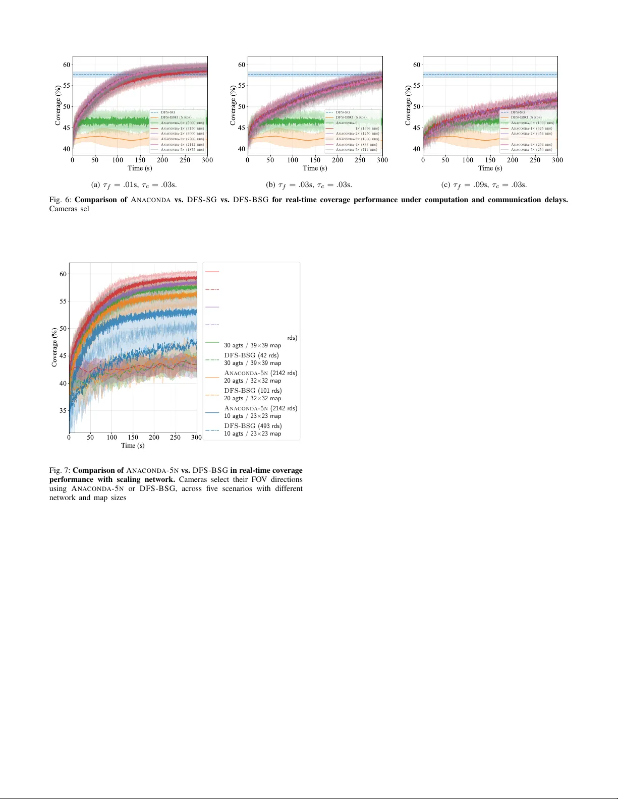
Self-Conﬁgurable Mesh-Networks for Scalable Distrib uted Submodular Bandit Optimization Zirui Xu, V asileios Tzoumas † Abstract —W e study how to scale distributed bandit submod- ular coordination under realistic communication constraints in bandwidth, data rate, and connectivity . W e are motivated by multi-agent tasks of active situational awareness in unknown, partially-observable, and r esource-limited envir onments, wher e the agents must coordinate thr ough agent-to-agent communica- tion. Our approach enables scalability by (i) limiting information relays to only one-hop communication and (ii) keeping inter -agent messages small, having each agent transmit only its own action information. Despite these inf ormation-access restrictions, our approach enables near-optimal action coordination by optimizing the agents’ communication neighborhoods over time, through distributed online bandit optimization, subject to the agents’ bandwidth constraints. Particularly , our approach enjoys an anytime suboptimality bound that is also strictly positive for arbitrary network topologies, even disconnected. T o prove the bound, we deﬁne the V alue of Coordination ( V oC ), an information- theoretic metric that quantiﬁes f or each agent the beneﬁt of information access to its neighbors. W e v alidate in simulations the scalability and near -optimality of our approach: it is observed to con verge faster , outperform benchmarks for bandit submodular coordination, and can even outperform benchmarks that are privileged with a priori knowledge of the en vironment. I . I N T R O D U C T I O N In the future, large-scale teams of distributed agents will be executing sensing-driv en tasks such as tar get tracking [ 1 ], en vironmental mapping [ 2 ], and area monitoring [ 3 ]. These collaborativ e tasks require the distributed agents to share their local observations—e xpand information access—to improve coordination performance. Howe ver , expanding information access is challenging due to the limited communication, computing, and sensing capabilities onboard each agent, and the above tasks often operate in unkno wn, unstructured, and dynamic en vironments. In more detail, sev eral challenges to scalability and optimality appear: (a) Limited communication bandwidth: Each agent can communicate with only a limited number of peers at a time, rather than with all physically reachable ones [ 4 ], [ 5 ]. (b) Finite data rate: Communication occurs via onboard radio modules with restricted data rates, ranging from as low as 0.25 Mbps ( e.g . , Digi XBee 3 Zigbee 3 [ 6 ]) to around 100 Mbps ( e.g. , Silvus T ech SL5200 [ 7 ]), far below the 0.8–1.5 Gbps commonly av ailable in e veryday W i-Fi 6 systems [ 8 ]. (c) Unguaranteed network connectivity: Agents may receive information only from those within a ﬁxed communication range or line of sight, meaning the communication graph is not guaranteed to remain connected [ 9 ]. † Department of Aerospace Engineering, Univ ersity of Michigan, Ann Arbor , MI 48109 USA; {ziruixu,vtzoumas}@umich.edu (d) Unstructured envir onment: The en vironment may be unknown a priori and partially observ able. Thus, the infor- mational value of each observation becomes kno wn only once the observation is made. This optimization setting corresponds to the bandit feedback model [ 10 ]. These challenges motiv ate distributed optimization prob- lems in bandit settings [ 10 ] for lar ge-scale tasks in robotics, control, and machine learning. Such joint optimization prob- lems often take the form of max a i,t ∈ V i , ∀ i ∈ N , ∀ t ∈ [ T ] T X t =1 f ( { a i,t } i ∈ N ) , (1) where T is the operation time-horizon, and at each time step t ∈ [ T ] , the agents N need to each select an action a i,t from its av ailable action set V i to collaborati vely maximize the unknown a priori objective function f : 2 Q i ∈N V i 7→ R that captures the task utility [ 2 ], [ 3 ], [ 11 ]–[ 21 ]. In information- gathering tasks, f is often submodular [ 22 ]: submodularity is a diminishing returns property , and it emanates due to the possible information overlap among the information gathered by the agents [ 11 ]. For example, in target monitoring with multiple cameras at ﬁxed locations, N is the set of cameras, V i is the av ailable directions the camera can choose, and f is the number of targets covered by the cameras’ collective ﬁeld of view (FO V). The cameras have no prior kno wledge of target locations and can observe them only when they fall within the cameras’ collectiv e FO V ; targets that remain uncov ered are therefore unkno wn to the cameras. As a result, the cameras can accurately ev aluate only the utility of the FO Vs they actually choose, which corresponds to the bandit feedback setting [ 10 ]. The optimization problem in eq. ( 1 ) is NP-hard ev en in known en vironments [ 23 ]. Polynomial-time algorithms with prov able approximation guarantees e xist. A classical example is the Sequential Greedy ( S G) algorithm [ 22 ], which achieves a 1 / 2 -approximation ratio. Since many multi-agent tasks, such as target tracking, collaborative mapping, and area monitoring, can be formulated as submodular coordination problems, S G and its v ariants ha ve been widely adopted across the controls, machine learning, and robotics communities [ 2 ], [ 3 ], [ 11 ]– [ 14 ], [ 16 ], [ 17 ], [ 19 ]–[ 21 ], [ 24 ]–[ 26 ]. In unknown en viron- ments instead, online variants of S G are proposed [ 1 ], [ 27 ]– [ 33 ], providing guaranteed suboptimality over the horizon T . Continuous-domain optimization techniques have also been lev eraged in the bandit setting by ﬁrst using the multilinear extension [ 34 ], to lift the discrete submodular function f to the continuous domain, then applying gradient/consensus-based techniques, and ﬁnally rounding back to the discrete domain to obtain a near-optimal solution [ 20 ], [ 32 ], [ 35 ]–[ 37 ]. Fig. 1: Information Access Matters: A Multi-Camera Area Monitoring Example. Consider a multi-camera area monitoring task where four cameras must coordinate their ﬁelds of vie w (FOVs) via distrib uted communication to maximize total coverage. As shown in (a), suppose that cameras 1–3 ha ve already ﬁxed their FO Vs (soft orange), and camera 4 must select its FO V from three predeﬁned options (dark red). While the optimal choice for camera 4 depends on the FOVs of all other three, its communication bandwidth allows it to receive information from at most two of them at any current time. The three possible communication neighborhood conﬁgurations and the corresponding FO V selections are demonstrated in (b)–(d), among which the design in (c) yields the highest coverage and therefore the optimal FOV decision. This example illustrates that intelligent information access—enabled by active neighborhood design (possibly over multiple time steps)—can optimize action coordination performance in distributed settings with limited communication resources. Howe ver , the algorithms above cannot scale as the network grows when challenges (a)–(d) exist simultaneously . In partic- ular , current distributed approaches, based on either sequential communication in the discrete domain [ 1 ], [ 2 ], [ 33 ] or repeated consensus iterations in the continuous domain [ 20 ], [ 24 ], [ 27 ]– [ 32 ], [ 35 ]–[ 37 ], assume instantaneous agent-to-agent commu- nication, i.e. , inﬁnite data rates. But if accounting for the limited data rates of onboard radio modules, per challenge (b), decision times of these methods can scale cubically in network size or ev en more [ 21 , T able 1]. This is due to: • Message size: The size of communication messages can scale proportionally with the number of agents. • Information r elay: Distrib uted agents use multi-hop relays to expand information access. In sum, under challenges (a)–(d), where instantaneous com- munication is infeasible and the en vironment is unknown, achieving both scalability and optimality requires restricting information access intelligently , via limiting message size and/or information relay , to balance the trade-off between decision time and decision optimality . Methods in [ 38 ], [ 39 ] lev erage communication quantization to shorten messages and ev aluate its ef fect on optimality . The framew ork in [ 40 ] reduces communication overhead by exploiting the sparsity of the underlying information dependence among agents and omitting information sharing between agents with lo w depen- dence accordingly . It also establishes the necessary conditions for con vergence. Howe ver , the approaches in [ 38 ]–[ 40 ] focus on con vex optimization. In discrete submodular optimization, the focus of this paper , current works [ 14 ]–[ 16 ] only perform f -agnostic communication restriction, i.e. , the topology de- signed will remain the same, independently of the f speciﬁed by the application. In more detail, [ 14 ]–[ 16 ] study a variant of S G with restricted information relay where each agent i receiv es information from only a subset rather than all of { 1 , . . . , i − 1 } as in the classical S G . 1 These works deri ve suboptimality bounds that scale in versely with the indepen- 1 In discrete submodular optimization, agents perform sequential commu- nication, where message complexity depends on the network topology . For example, in a line network, a message from agent i − 1 to i may aggregate information from all preceding agents { 1 , . . . , i − 1 } , whereas in a complete network it contains only agent i − 1 ’ s data, with other information transmitted through separate links. dence number of the resulting information-sharing topology , 2 and further propose a centralized information-sharing topol- ogy design method based on these bounds [ 16 ]. The recent algorithm in [ 21 ] restricts information access within one-hop neighbors, thus prohibiting relays and having each agent-to- agent message to contain information only about the agent that transmits it. It also enables partially parallelized action selection to reduce communication latency . Although [ 21 ] characterizes f -speciﬁc coordination performance, the bound is intractable to optimize even in hindsight, and therefore cannot support intelligent information access restriction. Contributions. W e provide a distrib uted multi-agent decision-making framework that enables both scalable and near-optimal action coordination in unknown environments under realistic communication constraints in bandwidth, data rate, and connectivity . Our approach enables scalability by (i) limiting information relays to only one-hop communication and (ii) keeping inter-agent messages small, having each agent transmit only its o wn action information. Despite these information-access restrictions, our approach improves the near-optimality bound of action coordination by optimizing the agents’ communication neighborhoods o ver time, through distributed online bandit optimization (subject to the agents’ bandwidth constraints)—the necessity for such information access optimization is demonstrated in Fig. 1 . T o our kno wledge, this is the ﬁrst rigorous approach that enables multi-agent networks to scale near-optimal coordina- tion by activ ely optimizing the restricted information access through acti ve communication topology self-conﬁguration. The approach is fully distrib uted: each agent jointly selects its action and designs its local communication neighborhood subject to its coordination neighborhood and bandwidth con- straints. The algorithm has the follo wing properties: a) Scalability: A NA C O N DA enjoys impro ved scalability under communication constraints by having a conv ergence time of O ( |N | 2 ) in sparse networks, accounting for informa- tion relay in multi-hop communication (Section V ). This is faster than existing methods ev en though they only consider known en vironments [ 21 , T able I]. In practice, the algorithm 2 This information-sharing topology is the Directed Acyclic Graph (D A G) deriv ed from the communication network. can conv ergence ev en faster , e.g . , only sublinearly in |N | in the area monitoring simulations (Section VII-D ). b) Anytime Self-Conﬁguration with Arbitr ary T opologies: A NA C O N DA enables each agent to adapt its communication neighborhood online according to the giv en f , resulting in coordination over a directed, time-varying, and potentially disconnected network. The fully distrib uted self-conﬁguration mechanism further allows agents to join or leav e the system without disrupting the co-optimization process. Our prior work [ 21 ], instead, does not optimize the network; [ 16 ] performs network design centrally without le veraging f ; and [ 1 ]–[ 3 ], [ 17 ], [ 19 ], [ 20 ], [ 24 ], [ 25 ], [ 33 ] require connected networks. c) Appr oximation P erformance: A N AC O N DA enjoys any- time, strictly positiv e, f -speciﬁc suboptimality bounds ag ainst an optimal solution of eq. ( 1 ) (Section IV ). The bounds capture the beneﬁt of information access for each agent and thus remain v alid under arbitrarily optimized communication topologies, regardless of global connectivity . In particular , Theorem 1 , along with our numerical ev aluations, v alidates that coordination performance improves through network op- timization, and Theorems 2 and 3 ensure that A N AC O N DA achiev es strictly positiv e performance guarantees at all times. The bounds in [ 14 ]–[ 16 ] are instead f -agnostic; the bound in our prior work [ 21 ] does not support network optimization; and [ 1 ]–[ 3 ], [ 17 ], [ 19 ], [ 20 ], [ 24 ], [ 25 ], [ 33 ] provide subopti- mality guarantees only under connected network assumptions. Numerical evaluations. W e v alidate A NAC O N D A through simulations of multi-camera area monitoring. The results ﬁrst show that the proposed information-driv en neighbor selection strategy outperforms typical baselines (nearest and random neighbors) in robotics and controls [ 21 ], [ 41 ], [ 42 ], with particularly large gaps in certain structured en vironments (Sec- tion VI ). Then, comparisons with state-of-the-art centralized and sequential methods ( D F S - S G and D F S - B S G ) under both idealized and realistic delay settings reveal a fundamental trade-off between coordination optimality and con ver gence speed, and highlight the importance of delay-aware ev aluation for real-time performance. Although the benchmarks require relaxed versions of the problem in eq. ( 1 ) to be applicable, A NA C O N DA still achie ves competitiv e or better coverage (Sections VII-A to VII-C ). Finally , large-scale simulations conﬁrm the scalability of A N AC O N DA : while benchmarks such as D F S - B S G incur prohibitive communication delays, A N A - C O N DA maintains a constant time per decision round and can scale sublinearly in network size in practice (Section VII-D ). W e ran all simulations using Python 3.11.7 on a W indows PC with an Intel Core i9-14900KF CPU @ 3.20 GHz and 64 GB RAM. The code is available at https://github.com/UM- iRaL/Self-conﬁgurable-network . Comparison with preliminary work [ 21 ], [ 43 ]. This paper extends our preliminary work [ 43 ] to include ne w theoretical results, extensiv e ev aluations, and proofs of all claims. W e introduce a tighter a priori bound (Theorem 1 ), a strictly positiv e a posteriori bound (Theorem 2 ), and a strictly pos- itiv e asymptotic bound (Theorem 3 ), and we comprehensively ev aluate the proposed algorithm across coordination perfor- mance, neighborhood design, and scalability metrics in area monitoring scenarios (Section VI ). This paper also extends the formulation in prior work [ 21 ] where communication neighborhoods are ﬁxed and constructed heuristically ( e.g. , via nearest neighbors). Here, we perform network optimization and demonstrate that the resulting conﬁgurations outperform nearest neighbors in area monitoring scenarios (Section VI ). I I . D I S T R I B U T E D C O O R D I N A T I O N A N D N E T W O R K C O - O P T I M I Z A T I O N W e present the problem formulation of Distributed Coor di- nation and Network Co-Optimization . W e use the notation: • V N ≜ Q i ∈ N V i is the cross product of sets {V i } i ∈ N . • [ T ] ≜ { 1 , . . . , T } for an y positive inte ger T . • f ( a | A ) ≜ f ( A ∪ { a } ) − f ( A ) is the marginal gain of set function f : 2 V 7→ R for adding a ∈ V to A ⊆ V . • |A| is the cardinality of a discrete set A . W e also lay down the follo wing framework about the agents’ communication network and the objectiv e function f . Communication network. The agents’ communication net- work G t = ( N , E t ) , ∀ t is undetermined a priori, where E t is the set of (directed) communication edges among agents N at time t . The goal of this work is for the agents to jointly optimize E t to enable con v ergence to a near -optimal solution to ( 1 ) despite distributed coordination. The network optimized by N can be directed and even disconnected . W e refer to the case where every agent receiv es information from all others as fully centralized , and the case where no agent receiv es information from any other as fully decentralized . Communication neighborhood. When a communication channel exists from agent j to agent i at time t , i.e. , ( j → i ) ∈ E t , then i can receiv e, store, and process information sent by j , and the set of all such j is i ’ s communication neighborhood , denoted as N i,t . Communication constraints. Each agent i can receiv e information from up to α i other agents at the same time due to onboard bandwidth constraints, i.e . , |N i,t | ≤ α i , ∀ t . Also, we denote as M i ⊆ N \ { i } the set of agents that can potentially send information to agent i —not all N \ { i } can reach agent i due to distance or obstacles: agent i can pick its neighbors by choosing at most α i agents from M i . W e refer to M i as agent i ’ s coor dination neighborhood ( N i,t ⊆ M i , ∀ t ). Deﬁnition 1 (Normalized and Non-Decreasing Submodular Set Function [ 22 ]) . A set function f : 2 V 7→ R is normalized and non-decreasing submodular if and only if • (Normalization) f ( ∅ ) = 0 ; • (Monotonicity) f ( A ) ≤ f ( B ) , ∀ A ⊆ B ⊆ V ; • (Submodularity) f ( s | A ) ≥ f ( s | B ) , ∀ A ⊆ B ⊆ V and s ∈ V . Intuitiv ely , if f ( A ) captures the number of tar gets tracked by a set A of sensors, then the more sensors are deployed, more or the same targets are covered; this is the non-decreasing property . Also, the marginal gain of tracked targets caused by deploying a sensor s dr ops when mor e sensors are already deployed; this is the submodularity property . Deﬁnition 2 (2nd-order Submodular Set Function [ 44 ], [ 45 ]) . f : 2 V 7→ R is 2nd-order submodular if and only if f ( s | C ) − f ( s | A ∪ C ) ≥ f ( s | B ∪ C ) − f ( s | A ∪ B ∪ C ) , (2) Algorithm 1: AlterN Ating COordination and Network Design Algorithm ( A NA C O ND A ) for Agent i Input: T ime horizon T ; agent i ’ s coordination neighborhood M i ; agent i ’ s communication bandwidth α i . Output: Action a i,t and communication neighborhood N i,t , ∀ t ∈ [ T ] . 1: N i, 0 ← ∅ , ∀ i ∈ N ; 2: for each time step t ∈ [ T ] do 3: a i,t ← A C T S E L ([ T ] , V i ) ; 4: N i,t ← N E I S E L ( a i,t , [ T ] , M i , α i ) ; 5: recei ve neighbors’ actions { a j,t } j ∈ N i,t and update A C T S E L (per lines 6-8) and N E I S E L (per lines 6-11); 6: end for for any disjoint A , B , C ⊆ V ( A ∩ B ∩ C = ∅ ) and s ∈ V . Intuitiv ely , if f ( A ) captures the number of targets tracked by a set A of sensors, then mar ginal gain of the marginal gains drops when more sensors are already deployed. Problem 1 (Distributed Coordination and Network Co-Op- timization) . At each t ∈ [ T ] , each agent i ∈ N selects a communication neighborhood N i,t of size up to α i and an action a i,t to solve the optimization problem max N i,t ⊆ M i , |N i,t | ≤ α i ∀ i ∈ N , ∀ t ∈ [ T ] max a i,t ∈ V i ∀ i ∈ N , ∀ t ∈ [ T ] T X t =1 f ( { a i,t } i ∈ N ) , (3) wher e (i) each ag ent i can coordinate with its neighbor s only , without any information about non-neighbor s, (ii) f : 2 V N 7→ R is a normalized, non-decreasing submodular , and 2nd-order submodular , and (iii) f is known via bandit feedback, in particular , each agent i can access the value of f ( A t ) only , ∀ A t ⊆ { a i,t } ∪ { a j,t } j ∈N i,t , once the ag ent has selected a i,t and r eceived { a j,t } j ∈N i,t fr om neighbors. Problem 1 captures the intrinsic coupling between coordina- tion performance and information access, as illustrated by the example in Figure 1 . The objective of this paper is to design the communication network topology that maximizes action coordination performance through solving Problem 1 . I I I . A LT E R NAT I N G C O O R D I N A T I O N A N D N E T W O R K - D E S I G N A L G O R I T H M ( A N AC O N D A ) W e present A N AC O N D A . A NA C O N DA approximates a solu- tion to Problem 1 by alternating the optimization for action coordination and communication neighborhood design. Since both action coordination and communication neighborhood de- sign take the form of adversarial bandit problems, we present ﬁrst the adversarial bandit (Section III-A ), then the algorithms A C T S E L (Section III-B ) and N E I S E L (Section III-C ). A. Adversarial Bandit Pr oblem The adversarial bandit problem in volv es an agent selecting a sequence of actions to maximize the total reward over a giv en number of time steps [ 10 ]. The challenge is that, at each time step, no action’ s reward is known to the agent a priori, and Algorithm 2: A C T S E L for Agent i Input: T ime horizon T and agent i ’ s action set V i . Output: Agent i ’ s action a i,t , ∀ t ∈ [ T ] . 1: η a i ← p 2 log |V i | / ( |V i | T ) ; 2: w 1 ←  w 1 , 1 , . . . , w |V i | , 1  ⊤ with w v , 1 = 1 , ∀ a ∈ V i ; 3: for each time step t ∈ [ T ] do 4: get distribution p t ← w t / ∥ w t ∥ 1 ; 5: draw action a i,t ∈ V i from p t ; 6: input a i,t to N E I S E L and recei ve neighbors’ actions { a j,t } j ∈N i,t ; 7: r a i,t ,t ← f ( a i,t | { a j,t } j ∈N i,t ) and normalize r a i,t ,t to [0 , 1] ; 8: ˆ r a, t ← 1 − 1 ( a i,t = a ) p a,t  1 − r a i,t ,t  , ∀ a ∈ V i ; 9: w a,t +1 ← w a,t exp ( η n i ˆ r a,t ) , ∀ a ∈ V i ; 10: end for after an action is selected, only the selected action’ s reward will become known. T o present the problem, we hav e: • V denotes the a vailable action set; • v t ∈ V denotes the agent’ s selected action at time t ; • r v t , t ∈ [0 , 1] denotes the re ward of selecting v t at time t . Problem 2 (Adversarial Bandit [ 10 ]) . Assume a horizon of T time steps. At each time step t ∈ [ T ] , the agent needs to select an action v t ∈ V suc h that the r e gr et Regret T ≜ max v ∈ V T X t =1 r v , t − T X t =1 r v t , t , (4) is minimized, where no actions’ r ewar ds are known a priori, and only the r ewar d r v t , t ∈ [0 , 1] becomes known to the agent after v t is selected. The goal of solving Problem 2 is to achiev e a sublinear Regret T , i.e. , Regret T /T → 0 for T → ∞ , since this implies that the agent asymptotically chooses optimal actions ev en though the rew ards are unknown a priori [ 10 ]. The most classical adv ersarial bandit algorithm E X P 3 [ 46 ] achiev es the goal above by obtaining a regret bound of ˜ O ( p |V | T ) , where ˜ O ( · ) hides log terms. During the past two decades, sev eral reﬁned adversarial bandit algorithms hav e emerged, including E X P 3 - I X for high-probability regret bounds via implicit exploration [ 47 ], E X P 3 + + for adaptation between stochastic and adversarial regimes [ 48 ], and T S A L L I S - I N F for minimax-optimal regret with improved adapti vity through Tsallis entropy regularization [ 49 ]. In this paper , we will formulate both action coordination and neighbor selection problems in the form of Problem 2 , and employ E X P 3 as the bandit solver without loss of generality . Alternativ e methods such as those mentioned abov e are also applicable ( e.g. , E X P 3 - I X was used in [ 43 ]). B. Action Coor dination W e introduce the A C T S E L algorithm and establish its per - formance guarantees. T o this end, we ﬁrst deﬁne the coordina- tion problem that A C T S E L addresses and relate it to Problem 2 for each agent. • A t ≜ { a i,t } i ∈N is the set of all agents’ actions at t ; • A OPT ∈ arg max a i ∈V i , ∀ i ∈N f ( { a i } i ∈N ) is the optimal actions for agents N that solve eq. ( 1 ). Intuitiv ely , each agent i ’ s goal at each time step t is to efﬁciently select an action a i,t that solves max a i,t ∈V i f ( a i,t | { a j,t } j ∈N i,t ) , (5) T o enable efﬁcienc y , the agents should ideally select actions simultaneously , unlik e ofﬂine algorithms such as Sequential Greedy [ 22 ] and Resource-A w are distrib uted Greedy [ 21 ] that employ (partially parallelized) sequential operations. But if they want to select actions simultaneously , { a j,t } j ∈N i,t will become known only after agent i selects a i,t and commu- nicates with N i,t . Therefore, computing the marginal gain is possible only in hindsight, once all agents’ decisions have been ﬁnalized for time step t . Thus, action selection for each agent aligns with the framew ork of Problem 2 , where the reward of selecting a i,t ∈ V i is r a i,t ,t ≜ f ( a i,t | { a j,t } j ∈N i,t ) , which becomes av ailable only after choosing a i,t . A C T S E L starts by initializing a learning rate η a i and a weight vector w t for all av ailable actions a ∈ V i (Algorithm 2 ’ s lines 1-2). Then, at each t ∈ [ T ] , it sequentially ex ecutes the following steps: 1) Compute probability distribution p t using w t (lines 3-4); 2) Select action a i,t ∈ V i by sampling from p t (line 5); 3) Send a i,t to N E I S E L and recei ve neighbors’ actions { a j,t } j ∈N i,t (line 6); 4) Compute rew ard r a i,t ,t , estimate re ward ˆ r a,t of each a ∈ V , and update weight w a,t +1 of each a ∈ V i (lines 7-9). 3 W e introduce the novel quantiﬁcation that ev aluates the beneﬁt of information access in solving Problem 1 . Deﬁnition 3 (V alue of Coordination ( V oC )) . Consider t ∈ [ T ] and agent i ∈ N with action a i,t and coor dination neighbor- hood M i . Agent i ’ s V alue of Coordination is deﬁned as: V oC f ,t ( a i,t ; N i,t ) ≜ f ( a i,t ) − f ( a i,t | { a j,t } j ∈N i,t ) , (6) wher e N i,t ⊆ M i is the communication neighborhood that i chooses to r eceive information fr om, |N i,t |≤ α i . V oC f ,t ( a i,t ; N i,t ) is thus an information theory metric sim- ilar to mutual information yet ov er the set function f . It represents the ov erlap between agent i and its communica- tion neighbors’ actions. Particularly , P T t =1 V oC f ,t ( a i,t ; N i,t ) ev aluates agent i ’ s beneﬁt in coordinating with N i,t ov er the horizon T . The larger is this v alue, the more related is the receiv ed information to the selected actions. Deﬁnition 4 (Curvature [ 50 ]) . The curvatur e of a normalized submodular function f : 2 V 7→ R is deﬁned as κ f ≜ 1 − min v ∈V f ( V ) − f ( V \ { v } ) f ( v ) . (7) 3 The coordination algorithms in [ 18 ]–[ 20 ] instruct the agents to select ac- tions simultaneously at each time step as A C T S E L , but they lift the coordination problem to the continuous domain and require each agent to kno w/estimate the gradient of the multilinear extension of f , which leads to a decision time at least one order higher than A CT S EL [ 21 ]. Algorithm 3: N E I S E L for Agent i Input: T ime horizon T ; agent i ’ s coordination neighborhood M i ; agent i ’ s communication bandwidth α i . Output: Agent i ’ s communication neighborhood N i,t , ∀ t ∈ [ T ] . 1: η n i ← p 2 log |M i | / ( |M i | T ) ; 2: z ( k ) 1 ← h z ( k ) 1 , 1 , . . . , z ( k ) α i , 1 i ⊤ with z ( k ) j, 1 = 1 , ∀ v ∈ M i , ∀ k ∈ [ α i ] ; 3: for each time step t ∈ [ T ] do 4: recei ve action a i,t from A C T S E L ; 5: for k = 1 , . . . , α i do 6: get distribution q ( k ) t ← z ( k ) t / ∥ z ( k ) t ∥ 1 ; 7: draw agent j ( k ) t ∈ M i from q ( k ) t ; 8: recei ve action a j ( k ) t ,t from j ( k ) t ; 9: r j ( k ) t ,t ← V oC f ,t ( a i,t ; { a j (1) t ,t , . . . , a j ( k ) t ,t } ) − V oC f ,t ( a i,t ; { a j (1) t ,t , . . . , a j ( k − 1) t ,t } ) and normalize r j ( k ) t ,t to [0 , 1] ; 10: ˆ r ( k ) j,t ← 1 − 1 ( j ( k ) t = j ) q ( k ) j,t  1 − r j ( k ) t ,t  , ∀ j ∈ M i ; 11: z ( k ) j,t +1 ← z ( k ) j, t exp ( η n i ˆ r ( k ) j,t ) , ∀ j ∈ M i ; 12: end for 13: N i,t ← { j k,t } k ∈ [ α i ] ; 14: end for Intuitiv ely , κ f measures how far f is from modularity: if κ f = 0 , then f ( V ) − f ( V \ { v } ) = f ( v ) , ∀ v ∈ V , i.e. , f is modular . In contrast, κ f = 1 in the extreme case where there exist v ∈ V such that f ( V ) = f ( V \ { v } ) , i.e. , v has no contribution in the presence of V \ { v } . Proposition 1 (Approximation Performance of A C T S E L ) . Over t ∈ [ T ] , a gents N can use A C T S E L to select actions {A t } t ∈ [ T ] such that T X t =1 f ( A t ) ≥ (1 − κ f ) T X t =1 " f ( A OPT ) + X i ∈N V oC f ,t ( a i,t ; N i,t ) # − ˜ O  |N | q | ¯ V | T  . (8) wher e | ¯ V | ≜ max i ∈N |V i | . Proposition 1 implies that A C T S E L ’ s performance increases for neighborhoods {N i,t } i ∈N with higher V oC f ,t ( a i,t ; N i,t ) . The proof appears in Appendix A. Lemma 1 (Monotonicity and Submodularity of V oC ) . Given an action a ∈ V i and a non-decr easing and 2nd-or der submodular function f : 2 V N 7→ R , then V oC f ,t ( a ; · ) is non- decr easing and submodular in the second ar gument. N E I S E L will next lev erage Lemma 1 to enable each agent to individually select its communication neighborhood that opti- mizes the approximation bound of A C T S E L (Proposition 1 ). C. Neighbor Selection W e no w present the N E I S E L algorithm and its performance guarantees for maximizing V oC . Particularly , we introduce the neighbor-selection problem that N E I S E L enables agents to solve in parallel and demonstrate that it aligns with Problem 2 . Since the suboptimality bound of A C T S E L in eq. ( 8 ) im- prov es as V oC f ,t ( a i,t ; N i,t ) increases, N E I S E L aims to enable each agent i to choose neighbors by solving the following cardinality-constrained maximization problem: max N i,t ⊆ M i , |N i,t | ≤ α i T X t =1 V oC f ,t ( a i,t ; N i,t ) , (9) where a i,t is gi ven by A C T S E L . This is a submodular maximization problem since we show in Lemma 1 that V oC f ,t ( a i,t ; N i,t ) is submodular in N i,t . But V oC f ,t ( a i,t ; N i,t ) is computable in hindsight only: { a j,t } j ∈N i,t become known only after agent i has selected and communicated with N i,t . Therefore, eq. ( 9 ) takes the form of cardinality-constrained bandit submodular maximization [ 1 ], [ 32 ], [ 51 ], which is an extension of Problem 2 to the multi-agent submodular setting. Solving eq. ( 9 ) using algorithms for Problem 2 will lead to exponential-running-time algorithms due to an exponen- tially large V per eq. ( 4 ) [ 51 ]. Therefore, N E I S E L instead extends [ 51 , Algorithm 2], which can solve eq. ( 9 ) in the full-information setting, to the bandit setting [ 1 ]. Speciﬁcally , N E I S E L decomposes eq. ( 9 ) to α i instances of Problem 2 , and separately solves each of them using E X P 3 . N E I S E L starts by initializing a learning rate η n i and α i weight vectors z ( k ) t , ∀ k ∈ [ α i ] , each determining the k -th selection in N i,t (Algorithm 3 ’ s lines 1-2). Then, at each t ∈ [ T ] , it sequentially executes the follo wing steps: 1) Receiv e action a i,t by A C T S E L (lines 3-4); 2) Compute distribution q ( k ) t using z ( k ) t , ∀ k ∈ [ α i ] (lines 5-6); 3) Select agent j ( k ) t ∈ M i as neighbor by sampling from q ( k ) t , and receiv e its action a j ( k ) t ,t , ∀ k ∈ [ α i ] (lines 7-8); 4) For each k ∈ [ α i ] , compute rew ard r j ( k ) t ,t associated with each j ( k ) t , estimate rew ard ˜ r ( k ) j,t of each j ∈ M i , and update weight z ( k ) j,t +1 of each j ∈ M i (lines 9-12). I V . S U B O P T I M A L I T Y G U A R A NT E E S W e show that A N AC O N DA ’ s approximation performance against the optimal solution to eq. ( 1 ) improves with the sum of all agents’ V oC , and is strictly positiv e anytime, ev en before con vergence. T o this end, we begin with an a priori bound validating that N E I S E L indeed improv es A NA C O N DA ’ s per- formance bound (Section IV -A ). W e then pro vide an anytime strictly positiv e a posteriori bound (Section IV -B ). Combining the ﬁrst two results, we ﬁnally present an asymptotic bound (Section IV -C ). All proofs appear in Appendix A. A. A Priori Bound T o present the a priori bound, we ﬁrst present the following deﬁnitions and lemmas that measure the performances of A C T S E L and N E I S E L . W e use the following notation: • κ I ,i ≜ max t ∈ [ T ] κ I ,i,t , where κ I ,i,t is the curvature of V oC f ,t ( a i,t ; · ) , ∀ t ∈ [ T ] . κ I ,i is independent of κ f ; • ρ ( κ, α ) ≜ κ − 1 [1 − (1 − κ/α ) α ] , where κ ∈ [0 , 1] and α ∈ N . Notice that 1 ≥ κ − 1 [1 − (1 − κ/α ) α ] α →∞ > κ − 1 (1 − e − κ ) κ → 1 ≥ 1 − e − 1 . The performances of A C T S EL and N E I S E L are measured by the following quantities: Deﬁnition 5 (Static Regret of Action Selection) . Given agent i has neighbors {N i,t } t ∈ [ T ] over the horizon [ T ] . At each time step t , suppose ag ent i selects an action a i,t . Then, the static r e gret of { a i,t } t ∈ [ T ] is deﬁned as A-Reg T ( { a i,t } t ∈ [ T ] ) ≜ max a ∈V i T X t =1 f ( a | { a j,t } j ∈N i,t ) − T X t =1 f ( a i,t | { a j,t } j ∈N i,t ) . (10) Deﬁnition 6 ( ρ ( κ I ,i , α i ) -Approximate Static Regret of Neigh- bor Selection) . Given agent i has actions { a i,t } t ∈ [ T ] over horizon [ T ] . At each time step t , suppose a gent i selects a set of neighbors N i,t ⊆ M i , |N i,t |≤ α i . Then, the ρ ( κ I ,i , α i ) - appr oximate static re gr et of {N i,t } t ∈ [ T ] is deﬁned as N-Reg ρ ( κ I ,i ,α i ) { a i,t } t ∈ [ T ] ( {N i,t } t ∈ [ T ] ) ≜ ρ ( κ I ,i , α i ) max N i,t ⊆M i , |N i,t |≤ α i T X t =1 V oC f ,t ( a i,t ; N i,t ) − T X t =1 V oC f ,t ( a i,t ; N i,t ) . (11) Deﬁnition 6 e valuates the suboptimality of {N i,t } t ∈ [ T ] against the optimal communication neighborhood that would hav e been selected if V oC f ,t ( a i,t ; · ) had been kno wn a priori, ∀ t ∈ [ T ] . The optimal v alue in eq. ( 11 ) is discounted by ρ ( κ I ,i , α i ) since the problem in eq. ( 9 ) is NP-hard to solv e with an approximation factor greater than ρ ( κ I ,i , α i ) ev en when V oC f ,t ( a i,t ; · ) is known a priori [ 50 ]. Lemma 2 (Suboptimality Guarantee of A C T S E L ) . Con- sider horizon [ T ] . If agent i has a sequence of neighbors {N i,t } t ∈ [ T ] , re gar dless of how the y ar e selected, then using A C T S E L , ag ent i can choose actions { a i,t } t ∈ [ T ] such that A-Reg T ( { a i,t } t ∈ [ T ] ) ≤ ˜ O  p |V i | T  , (12) given the learning rate is set as η a i = p 2 log |V i | / ( |V i | T ) . Lemma 3 (Suboptimality Guarantee of N E I S E L ) . Consider horizon [ T ] . If ag ent i has a sequence of actions { a i,t } t ∈ [ T ] , r e gardless of how the y are selected, then using N E I S E L , agent i can choose neighbors {N i,t } t ∈ [ T ] such that N-Reg ρ ( κ I ,i ,α i ) { a i,t } t ∈ [ T ] ( {N i,t } t ∈ [ T ] ) ≤ ˜ O  α i p |M i | T  , (13) given the learning rate set as η n i = p 2 log |M i | / ( |V i | T ) . Now we present the a priori bound of A N AC O N DA . Theorem 1 (A Priori Approximation Performance) . Using A NA C O N DA , each agent i selects actions { a i,t } t ∈ [ T ] and 0 1 Curv ature 5 f 0 1 Asymptotic Bound - = 0 0 1 Curv ature 5 f 0 1 Asymptotic Bound 0 < - < 1 0 1 Curv ature 5 f 0 1 Asymptotic Bound - = 1 0 1 Curv ature 5 f 0 1 Asymptotic Bound - > 1 (1 ! 1 = - ; 1 = - ) A Priori (Thm 1) A Posteriori (Thm 2) Combined (Thm 3) Fig. 2: Asymptotic approximation bounds of A NAC O N DA . As T → ∞ , the bounds provided by Theorems 1 to 3 are sho wn with v arying ranges of κ f and achieved β (deﬁned in eq. ( 18 )). The a priori bound (red) varies with the sum of all agents’ V oC ; the a posteriori bound (orange) decreases as β increases; and the combined bound (green) takes the maximum of the a priori lower bound and the a posteriori bound. communication neighborhoods {N i,t } t ∈ [ T ] that guarantee: E [ f ( A t )] ≥ (1 − κ f ) f ( A OPT ) + κ f (1 − κ f ) ρ ( κ I , ¯ α ) × X i ∈N E  V oC f ,t ( a i,t ; N ⋆ i ( { a i,t } t ∈ [ T ] ; α i , M i ))  − ˜ O  |N | q  ¯ α 2 | ¯ M| + | ¯ V |  /T  , (14) wher e κ I ≜ max i ∈N κ I ,i , ¯ α ≜ max i ∈N α i , | ¯ V | ≜ max i ∈N |V i | , | ¯ M| ≜ max i ∈N |M i | , κ f , κ I ∈ [0 , 1] , ρ ( κ I , ¯ α ) ∈ [1 − 1 /e, 1] , and N ⋆ i ( { a i,t } t ∈ [ T ] ; α i , M i ) ⊆ M i is the op- timal communication neighborhood that solves eq. ( 9 ) given { a i,t } t ∈ [ T ] subject to α i . The expectation is due to the algo- rithm’ s internal randomness. Theorem 1 implies that as T → ∞ , the a priori approxi- mation ratio spans the interv al between fully centralized and fully decentralized coordination in accordance to V oC , and the spectrum is depicted in red in Fig. 2 . In particular , when the network is fully centralized with all agents listening to all others, i.e. , N i,t ≡ N \ { i } , E [ f ( A t )] ≥ 1 1 + κ f f ( A OPT ) − ˜ O  |N | q | ¯ V | /T  , (15) where the guaranteed 1 / (1 + κ f ) bound is near-optimal [ 50 ]. When the network is fully decentralized with no agent listen- ing to any others, i.e. , N i,t ≡ ∅ , E [ f ( A t )] ≥ (1 − κ f ) f ( A OPT ) − ˜ O  |N | q | ¯ V | /T  , (16) where 1 − κ f is the w orst-case bound achie ved by A NA C O N DA . B. A P osteriori Bound W e provide an a posteriori bound for A N AC O N DA that is strictly positiv e, even for ﬁnite T . Theorem 2 (A Posteriori Approximation Performance) . Using A NA C O N DA , each agent i ∈ N selects { a i,t } t ∈ [ T ] and {N i,t } t ∈ [ T ] that guarantee: E [ f ( A t )] ≥ 1 1 + β κ f + ˜ O  |N | p | ¯ V | /T  f ( A OPT ) , (17) wher e β ≜ E  P i ∈N f ( a i,t | { a j,t } j ∈N i,t )  E [ f ( A t )] ∈ [0 , ∞ ) (18) is computable after A NA C O N DA terminates. The e xpectation is due to the algorithm’s internal randomness. The bound is depicted in Fig. 2 in orange for varying ranges of β . Since E [ f ( A t )] > 0 , then β < ∞ , and Theorem 2 implies that A N AC O N DA always achieves a strictly positiv e asymptotic approximation ratio: E [ f ( A t )] T →∞ ≥ 1 1 + β κ f f ( A OPT ) > 0 . (19) Moreov er, if β = 0 , i.e. , each agent’ s selected action fully ov erlaps with its neighbors’ selected actions, then A N AC O N DA is asymptotically optimal: E [ f ( A t )] T →∞ ≥ f ( A OPT ) . (20) Finally , if 0 ≤ β ≤ 1 , then A NA C O N DA asymptotically outperforms the bound of Sequential Greedy [ 22 ]: E [ f ( A t )] T →∞ ≥ 1 1 + β κ f f ( A OPT ) ≥ 1 1 + κ f f ( A OPT ) . (21) This last scenario is guaranteed to occur when, e.g. , there exists an order of the agents such that [ i − 1] ⊆ N i,t , ∀ i, ∀ t . C. Combined Asymptotic Bound Combining Theorems 1 and 2 , we get: Theorem 3 (Asymptotic Approximation Performance) . A N A - C O N DA asymptotically achieves: E [ f ( A t )] f ( A OPT ) T →∞ ≥ max  1 − κ f , 1 1 + β κ f  > 0 , (22) wher e κ f ∈ [0 , 1] and β ∈ [0 , ∞ ) . The bound is depicted in Fig. 2 in green. V . D E C I S I O N T I M E A N A L Y S I S W e present the conv ergence time of A N AC O N DA by an- alyzing its computation and communication complexity , ac- counting for the delays due to function ev aluation and the transmission of messages under realistic communications. • τ f is the time required for one e valuation of f ; • τ c is the time for agent i to transmit the information about one action to agent j , without loss of generality , for all ( i → j ) ∈ E t , ∀ t . Theorem 4 (Conv ergence Time) . A N AC O N DA conver ges in O  ( τ f ¯ α + τ c ) ( ¯ α 2 | ¯ M| + | ¯ V | ) |N | 2 / ϵ  time. In sparse networks, the following corollary holds: 20 40 60 80 100 Camera Density (square unit/camera) 0 10 20 Co verage Impro vement (%) NeiSel vs. Random Neighbors NeiSel vs. Nearest Neighbors Fig. 3: Comparison of neighbor selection strategies with varying network density . Across 20 MC trials each with 2000 decision rounds, we compare N E I S E L with two benchmark strategies, Nearest Neighbors and Random Neighbors. W e tune the network density by varying the map area while ﬁxing the network size at 20 agents: as the camera density grows, the network becomes sparser . Corollary 1 (Con vergence T ime for Sparse Networks) . In sparse networks, wher e |M i | = o ( |N | ) , ∀ i ∈ N , A NA C O N DA con ver ges in O  ( τ f ¯ α + τ c ) | ¯ V | |N | 2 / ϵ  time. The proof appears in Appendix B. V I . N E C E S S I T Y F O R N E T W O R K O P T I M I Z A T I O N : N U M E R I C A L E V A L UA T I O N I N A R E A M O N I T O R I N G In this section, we demonstrate that optimizing the network topology , per A NA C O N DA , leads to improved coordination performance compared to heuristics for network design, such as the nearest and random selection that are typically used in controls and robotics [ 21 ], [ 41 ], [ 42 ]. In particular, we compare the proposed N E I S E L (Algorithm 3 ) with two heuris- tic strategies, Near est Neighbors and Random Neighbor s , in simulated 2D area-monitoring scenarios. The results show that N E I S E L consistently outperforms the benchmarks across different network densities (Fig. 3 ), and that while nearest- neighbor heuristic is quite misleading in certain structured en- vironments, N E I S E L can conﬁgure the optimal communication neighborhood (Fig. 4 ). W e defer the description of the former simulations to Appendix V and describe the latter below . In more detail, eight cameras are deployed to monitor four street blocks as shown in Fig. 4 . Under α i = 1 for all i ∈ N , the optimal neighbor for each camera is the one positioned opposite its corresponding street block so as to minimize FO V ov erlap. The results, shown in Fig. 4 and T able I , indicate that N E I S E L outperforms the two heuristic baselines by 27 . 2% and 11 . 5% in mean cov erage, respectiv ely . W e next describe the simulation setup, compared algorithms, and results. Setup. En vir onment: The environment is a 110 × 40 map with four 20 × 40 street blocks to monitor, as in Fig. 4 . Agents: Eight cameras are located on the boundaries of street blocks with locations (0 , 20) , (20 , 20) , (30 , 20) , (50 , 20) , (60 , 20) , (80 , 20) , (90 , 20) , and (110 , 20) . They all hav e large enough communication ranges c i such that M i = N \ { i } , ∀ i ∈ N . Actions: All cameras i ∈ N hav e FO V radius r i = 20 and A O V θ i = π / 2 , with direction a i,t chosen from the 16 cardinal directions, ∀ t . Each camera i is considered una ware of V j , j ∈ N \ { i } . Thus, the cameras hav e to communicate to know about one another’ s action information. Communication Network: The emergent time-v arying communication network G t can be directed and disconnected. At each decision round t , each camera i will ﬁrst ﬁnd its coordination neighborhood T ABLE I: Comparison of coverage performance (%) in the urban scenario as in Fig. 4 with different neighbor selection strate gies. The best coverage performance is in bold . Metric Nearest Neighbors Random Neighbors Ours Mean ± Std (%) 56.53 ± 4.57 64.47 ± 6.07 71.89 ± 7.36 Min (%) 35.56 ( t =1 ) 37.94 ( t =113 ) 39.72 ( t =169 ) Max (%) 71.09 ( t =2484 ) 72.56 ( t =895 ) 77.25 ( t =619 ) M i ≜ { j } ∥ x j − x i ∥≤ c i , j ∈ N \{ i } , where c i is i ’ s communication range. Then, it will select communication neighborhood N i,t from M i , following a strategy that will be determined by different compared algorithms. Once N i,t is conﬁgured by all i ∈ N , then G t is deﬁned. Objective Function: f ( { a i,t } i ∈N ) is the total area of interest covered by the cameras N when they select { a i,t } i ∈N as their FO V directions. f is pro ved to be submodular [ 3 ]. Perf ormance Metrics. W e ev aluate the achieved coverage of street blocks of the algorithms ov er 3000 decision rounds. Compared Algorithms. W e e valuate the following bench- marks, all selecting one neighbor per camera at each decision round, i.e. , α i = 1 for all i ∈ N : (i) A N AC O N DA : Our algorithm will follo w the process described in Section III . That is, at each round, the agents will each ﬁrst sample its action a i,t ∈ V i per A C T S E L and neighbors N i,t ⊆ M i per N E I S E L . Then, they will each communicate with N i,t and use the recei ved information to update the two bandit algorithms. (ii) A C T S E L + Nearest Neighbors: Action selection follows A NA C O N DA , while each camera i will always ha ve the same closest agent j ∈ M i as its neighbor . (iii) A C T S E L + Random Neighbors: Action selection follows A NA C O N DA , while each camera i will uniformly resample its neighbor from M i at each decision round. Results. W e observe that network optimization via N E I S E L increases both cov erage performance and con ver gence speed, as shown in Fig. 4 . In particular, A N AC O N D A outperforms the two benchmarks in all aspects of mean, minimum, and maximum coverage. It improves the benchmarks by (71 . 89% / 56 . 53% − 1 =)27 . 2% and (71 . 89% / 64 . 47% − 1 = )11 . 5% in the mean cov erage, respecti vely (T able I ). More- ov er, N E I S E L con ver ges to the optimal network conﬁguration after ∼ 1000 rounds, and then A C T S E L also con ver ges to the optimal coverage performance (77.25%) after ∼ 1800 rounds (Fig. 4 (c)). In contrast, we do not observe any conv ergence for the nearest neighbor selection (Fig. 4 (a)), and the con vergence appears slower for random neighbor selection after ∼ 2400 rounds, with a suboptimal coverage performance (72.56%). The reason why random neighbor selection performs better than nearest neighbor selection is that the latter will alw ays select the same neighbors, thus nev er choose the optimal conﬁguration. In contrast, random selection can happen to pick the optimum by chance, thus pro viding better performance. V I I . N U M E R I C A L E V A L U A T I O N I N A R E A M O N I T O R I N G While much of the distributed optimization literature ana- lyzes computation and communication complexities, it rarely considers how the resulting delays inﬂuence the algorithm’ s practical optimality ov er time. In time-critical applications, howe ver , the ability to make rapid decisions is essential, and 0 20 40 60 80 100 X 0 20 40 Y FOV Placement and Network Self-Configuration 1 2 3 4 5 6 7 8 0 500 1000 1500 2000 2500 3000 Decision Round 40 50 60 70 80 Coverage (%) Coverage Evolution (a) A C T S EL + Nearest neighbors. 0 20 40 60 80 100 X 0 20 40 Y FOV Placement and Network Self-Configuration 1 2 3 4 5 6 7 8 0 1000 2000 3000 Decision Round 40 50 60 70 80 Coverage (%) Coverage Evolution (b) A C T S EL + Random neighbors. 0 20 40 60 80 100 X 0 20 40 Y FOV Placement and Network Self-Configuration 1 2 3 4 5 6 7 8 0 500 1000 1500 2000 2500 3000 Decision Round 40 50 60 70 80 Coverage (%) Coverage Evolution (c) A C T S EL + N E I S E L ( A NAC O N DA ). Fig. 4: Comparison of neighbor selection strategies in a structured envir onment. Three algorithms are compared with the same action selection strategy A C T S EL but different neighbor selection strategies ( N EI S E L vs. nearest neighbors vs. random neighbors) in the same structured en vironment. computation and communication delays directly decide ho w many coordination rounds can be completed within a ﬁnite time horizon. As a result, an algorithm with a lower theoretical bound b ut higher decision frequency may outperform another with a higher bound but lo wer frequency , and thus delay-aw are ev aluation is crucial for revealing such ef fects. T o this end, in the section, we demonstrate the beneﬁts of A NA C O N DA by comparing it with benchmarks under two settings, i.e. , with and without communication and computa- tion delays. In particular , A NA C O N DA outperforms because it runs fast under delays. The simulation results, summarized in Figs. 5 – 7 and T able II , highlight the following insights: • A NA C O N DA achiev es competitiv e or improv ed perfor- mances to benchmarks, with and without delays, even though the benchmarks ar e tasked with easier versions of the pr oblem that A NA C O N DA solves and have higher performance bounds (Sections VII-B to VII-D ). • A NA C O N DA is observed to scale sublinearly in |N | under delays, in contrast to the benchmark that has almost no beneﬁt in network growth. (Section VII-D ). The common simulation setup is the same as Section VI . W e ne xt detail the benchmark algorithms (Section VII-A ) and comparison results without delays (Section VII-B ), with delays (Section VII-C ), and scalability under delays (Section VII-D ). A. Compar ed Algorithms W e compare the follo wing three algorithms. a) A NA C O N DA with differ ent communication neigh- borhood sizes: W e test A NA C O N DA varying the maxi- mum communication neighborhood size |N i,t |≤ α i , namely A NA C O N DA - α i N , where α i ∈ { 0 , . . . , 5 } . b) D F S - S G that requir es a (strongly) connected network and a known en vir onment [ 25 ]: W e test D F S - S G in terms of its achie ved objectiv e value after one round of multi- agent decisions. The of ﬂine algorithm is an implementation with communication speciﬁcations of S G for submodular maximization, which uses a DFS-based method to distribu- tiv ely determine the next agent ov er the (strongly) connected communication network. Therefore, the problem solved by D F S - S G is a relaxed version of Problem 1 where f is known and a connected communication network is giv en. D F S - S G enjoys the same 1 / (1 + κ f ) suboptimality bound as S G [ 22 ] and has a worst-case O ( τ c |N | 3 ) decision time. The proof of decision time appears in Appendix C. c) D F S - B S G that r equires a (strongly) connected net- work: W e test D F S - B S G in terms of its achiev ed objectiv e value and con vergence speed across multiple rounds of multi- agent decisions. The bandit algorithm is an implementation with communication speciﬁcations of B S G [ 1 ] that, similarly to A NA C O N DA , also decomposes multi-agent online decision- making into single-agent problems. But different from A N A - C O N DA , per D F S - B S G , (i) each agent i ’ s action selection re- ward is f ( a i,t | { a j,t } j ∈ [ i − 1] ) instead of f ( a i,t | { a j,t } j ∈N i,t ) , ∀ t , and (ii) computating rewards is enabled by the sequen- tial communication over all agents in a DFS-based order . 4 The problem solved by D F S - B S G is a relaxed version of Problem 1 where a connected communication network is giv en. D F S - B S G enjoys the same suboptimality bound as A NA C O N DA in the fully centralized case per Theorem 1 , and thus upon con ver gence, D F S - B S G has the same guarantee as D F S - S G. It requires O  ( τ f | ¯ V | |N | 2 + τ c |N | 5 ) | ¯ V | / ϵ  time to conv erge in a directed network. The proofs of suboptimality guarantees and decision time appear in Appendix D. When implementing the algorithms abov e in each MC trial, we ﬁrst let each agent i construct M i within the given communication range c i . Then, while each agent actively selects neighbors N i,t ⊆ M i with A N AC O N D A , it will directly take N i,t ≡ M i , ∀ t with D F S - S G and D F S - B S G . Although A NA C O N DA can accommodate arbitrary networks, we need to choose a not too small c i to ensure the resulting network is connected for D F S - S G and D F S - B S G . B. Comparison with No Delays: Coverage vs. Decision Round T o demonstrate the beneﬁt of information access to the sub- optimality of A N AC O N DA , we e valuate the above algorithms omitting computation and communication delays across four scenarios. (Fig. 5 ). Each scenario is assessed ov er 20 MC trials, where D F S - S G is executed for a single decision round and all other algorithms are run for 4000 rounds. 4 In [ 1 ], the B S G algorithm uses E X P 3 ⋆ - S IX as the single-agent algorithm that provides bounded tracking regret in dynamic environments. In this paper, although we instead consider static regret and adopt E X P 3 , the sequential communication scheme and decision time of B S G are not altered. 0 1000 2000 3000 4000 Decision Round 40 45 50 55 60 Coverage (%) (a) communication range = 10 0 1000 2000 3000 4000 Decision Round 40 45 50 55 60 Coverage (%) (b) communication range = 16 0 1000 2000 3000 4000 Decision Round 40 45 50 55 60 Coverage (%) (c) communication range = 30 0 1000 2000 3000 4000 Decision Round 40 45 50 55 60 Coverage (%) (d) communication range = 80 DFS-SG DFS-BSG Ana cond a-0n Ana cond a-1n Ana cond a-2n Ana cond a-3n Ana cond a-4n Ana cond a-5n Fig. 5: Comparison of A N AC ON DA , D F S -S G , and D F S- B S G for area monitoring without computation and communication delays. Cameras select their FO V directions using A N AC ON DA with maximum communication neighborhood sizes in { 0 , . . . , 5 } , or using D F S - SG or D F S -B S G. From (a) to (d), the communication range c i for all cameras i ∈ N increases from 10 to 16 to 20 to 80, and thus expanding each camera’ s coordination neighborhood M i growing from a small locality to the full set N \ i . D F S -S G is executed for a single decision round, whereas the other algorithms are run for 4000 rounds. Results are av eraged over 20 Monte Carlo trials. Setup. Envir onment: A static 50 × 50 map. Agents: There exist 50 cameras. The communication ranges c i ∈ { 10 , 16 , 30 , 80 } across the four scenarios. In each MC trial, the location x i of each camera i ∈ N is uniformly sampled in [0 , 50] 2 . Actions: Direction a i,t is chosen from the 16 cardinal directions, ∀ t , with FO V radius r i = 8 and A O V θ i = π / 3 . Results. The simulation results are presented in Fig. 5 , where we observ e a trade-of f of A N AC O N D A between cen- tralization and decentralization, where increasing α i or c i generally impro ves coverage after con ver gence but at the cost of more decision rounds. Both parameters follow the principle of diminishing marginal returns due to the submodularity of V oC : while larger α i and c i values enhance the agents’ information access, the gains ev entually become incremental. Furthermore, larger c i values signiﬁcantly increase the number of decision rounds required to con ver ge, meaning that highly centralized conﬁgurations may underperform compared to the benchmarks in shorter time horizons. Moreover , A N AC O N DA consistently achie ves improv ed asymptotic cov erage ov er these benchmarks as long as α i or c i are not too small, suggesting that intermediate parameter values, such as c i = 16 , offer the most effecti ve balance between real-time con ver gence and long-term performance. W e conjecture that A NA C ON D A ’ s improv ed performance arises from richer information mixing enabled by the time-v arying communication neighborhoods, as opposed to the benchmarks’ sequential information passing. C. Comparison with Delays: Coverage vs. Actual T ime W e compare A N AC O N DA with D F S - S G and D F S - B S G in 20 MC trials under three delay conﬁgurations ( τ f , τ c ) ∈ { ( . 01 s , . 03 s ) , ( . 03 s , . 03 s ) , ( . 09 s , . 03 s ) } , capturing different computation and communication capabilities. Each trial is carried out over a ﬁxed 300 s time horizon. Setup. The setup is identical to that in Fig. 5 (b), with the communication range c i = 16 for all cameras i ∈ N . Results. The simulation results are presented in Fig. 6 and T able II where we observe the following for A N AC O N DA : {A NA C O N DA demonstrates a better performance than D F S - B S G and can outperform D F S - S G after conv ergence. The reason is that A NA C O N DA decides actions much faster than D F S - B S G in large netw orks, which means much more deci- sion rounds in a ﬁxed time horizon. T ABLE II: Comparison of average cov erage performance (%) within 300 s across three scenarios with different delay conﬁgurations (Fig. 6 ). The highest value in each scenario is highlighted in bold . Algorithm Coverage (%) τ f = . 01 s , τ c = . 03 s τ f = . 03 s , τ c = . 03 s τ f = . 09 s , τ c = . 03 s D FS - BS G 42.19 ± 1.83 41.96 ± 1.98 42.30 ± 2.20 A NAC O ND A - 0 N 47.33 ± 1.84 46.52 ± 1.92 46.78 ± 1.77 A NAC O ND A - 1 N 58.27 ± 1.22 56.13 ± 1.77 52.17 ± 1.68 A NAC O ND A - 2 N 58.75 ± 1.18 56.75 ± 1.28 51.68 ± 1.90 A NAC O ND A - 3 N 59.05 ± 0.89 57.10 ± 1.04 51.73 ± 0.91 A NAC O ND A - 4 N 59.08 ± 0.82 56.20 ± 1.57 50.12 ± 0.93 A NAC O ND A - 5 N 59.12 ± 1.01 55.72 ± 1.32 49.99 ± 1.73 Increasing the neighborhood size α i presents a trade-off for A NA C O N DA : although larger neighborhoods theoretically offer higher asymptotic coverage, they also increase com- putation time per round, resulting in fewer decision cycles within a ﬁxed time horizon. For example, in Fig. 6 (a)–(c), the best-performing communication neighborhood sizes within the 300s windo w are α i = 5 , 3 , and 1 , respectiv ely , rather than always 5 (T able II ). This “no free neighbor” dynamic, characterized by a cubic growth in con vergence time relati ve to α i , means that smaller neighborhood sizes can yield better performance in a ﬁxed horizon. D. Scalability W e ﬁnally compare the real-time co verage performance of A NA C O N DA - 5 N and D F S - B S G over 20 MC trials as the network size scales across ﬁve scenarios with varying numbers of cameras and map sizes. Each trial is executed ov er a ﬁxed time horizon of 300 s with ( τ f , τ c ) = (0 . 01 s , 0 . 01 s ) . Setup. The ﬁ ve scenarios contain { 10 , 20 , 30 , 40 , 50 } cam- eras deployed in maps of sizes { 23 2 , 32 2 , 39 2 , 45 2 , 50 2 } , re- spectiv ely . These conﬁgurations maintain an approximately constant camera density , with each camera cov ering roughly 50 square units on average. Across all scenarios, the commu- nication range is ﬁxed at c i = 16 for all cameras i ∈ N . Results. A NA C O N DA scales despite imperfect communica- tion; D F S - B S G does not. Per Fig. 7 , when the network size increases from 10 to 50 agents, A N AC O N DA consistently ex- ecutes 2142 rounds, o wing to its ﬁxed per -round computation and communication load (Proposition 5 ), and the con ver gence time grows from 100s to 200s, which is a sublinear growth in |N | . In contrast, the number of rounds completed by D F S - B S G declines from 493 to just 15, because each round requires sequential communication across the entire network. 0 50 100 150 200 250 300 T ime (s) 40 45 50 55 60 Coverage (%) DFS-SG DFS-BSG (5 rds) Ana cond a-0n (5000 rds) Ana cond a-1n (3750 rds) Ana cond a-2n (3000 rds) Ana cond a-3n (2500 rds) Ana cond a-4n (2142 rds) Ana cond a-5n (1875 rds) (a) τ f = . 01 s, τ c = . 03 s. 0 50 100 150 200 250 300 T ime (s) 40 45 50 55 60 Coverage (%) DFS-SG DFS-BSG (5 rds) Ana cond a-0n (2500 rds) Ana cond a-1n (1666 rds) Ana cond a-2n (1250 rds) Ana cond a-3n (1000 rds) Ana cond a-4n (833 rds) Ana cond a-5n (714 rds) (b) τ f = . 03 s, τ c = . 03 s. 0 50 100 150 200 250 300 T ime (s) 40 45 50 55 60 Coverage (%) DFS-SG DFS-BSG (5 rds) Ana cond a-0n (1000 rds) Ana cond a-1n (625 rds) Ana cond a-2n (454 rds) Ana cond a-3n (357 rds) Ana cond a-4n (294 rds) Ana cond a-5n (250 rds) (c) τ f = . 09 s, τ c = . 03 s. Fig. 6: Comparison of A NAC O N DA vs. D F S - SG vs. D F S- B S G for r eal-time coverage perf ormance under computation and communication delays. Cameras select their FO V directions using A NAC O N DA with maximum communication neighborhood sizes in { 0 , . . . , 5 } , or using D F S - SG or D F S- B S G. From (a) to (b) to (c), the time τ f for one function evaluation increases relative to the delay τ c for transmitting one action through a communication link, with the ratio τ f /τ c taking values 1 / 3 , 1 , and 3 . D F S - SG is executed for a single decision round, whereas the other algorithms are run for a ﬁxed duration of 300 seconds. Under different delay conﬁgurations, the algorithms complete dif ferent numbers of decision rounds within this time window . Results are av eraged over 20 Monte Carlo trials. 0 50 100 150 200 250 300 T ime (s) 35 40 45 50 55 60 Coverage (%) Ana cond a-5n (2142 rds) 50 agts / 50 × 50 map DFS-BSG (15 rds) 50 agts / 50 × 50 map Ana cond a-5n (2142 rds) 40 agts / 45 × 45 map DFS-BSG (24 rds) 40 agts / 45 × 45 map Ana cond a-5n (2142 rds) 30 agts / 39 × 39 map DFS-BSG (42 rds) 30 agts / 39 × 39 map Ana cond a-5n (2142 rds) 20 agts / 32 × 32 map DFS-BSG (101 rds) 20 agts / 32 × 32 map Ana cond a-5n (2142 rds) 10 agts / 23 × 23 map DFS-BSG (493 rds) 10 agts / 23 × 23 map Fig. 7: Comparison of A N AC O ND A - 5 N vs. D FS - B S G in real-time cov erage performance with scaling network. Cameras select their FO V directions using A N AC O ND A -5 N or D F S - BS G , across ﬁve scenarios with different network and map sizes. T o k eep the camera density constant, the map size scales linearly from 23 × 23 to 50 × 50 as the network size ranges from 10 to 50 . Results are av eraged over 20 Monte Carlo trials, each with a ﬁxed 300 s time window under delays ( τ f , τ c ) = ( . 01 s , . 01 s ) . V I I I . C O N C L U S I O N W e presented A NA C O N DA , a scalable frame work for dis- tributed submodular coordination in multi-agent systems op- erating in unknown en vironments under realistic commu- nication constraints. A N AC O N D A achie ves scalability while maintaining near-optimal action coordination by intelligently limiting communication, regardless of global connectivity . W e introduced a novel metric, V oC , that quantiﬁes the beneﬁt of information access for coordination. By optimizing V oC , the framew ork enables intelligent information limitation through communication neighborhood design. The suboptimality guar- antees showed that A N AC O N DA ’ s coordination performance improv es with the sum of all agents’ V oC , and is anytime non-trivial ev en prior to con ver gence. Extensiv e simulations in multi-camera area monitoring against state-of-the-art bench- marks supported the theoretical analysis and illustrated A NA - C O N DA ’ s beneﬁt in coordination performance, neighborhood design, and scalability , together with a fundamental trade-of f between coordination optimality and con ver gence speed under realistic communication latency . Future work. While A N AC O N DA demonstrates improv e- ment in decision time compared to benchmarks for unknown en vironments, for mobile-robot applications, we will work to accelerate it to O ( |N | ) decision time, le veraging the tools in [ 52 ]. Moreov er , while the coordination neighborhood M i is currently considered static, it can be dynamic for mobile robots. T o this end, we will also handle dynamic coordination neighborhoods, i.e. , M i,t , with guaranteed performances. R E F E R E N C E S [1] Z. Xu, X. Lin, and V . Tzoumas, “Bandit submodular maximization for multi-robot coordination in unpredictable and partially observable en vironments, ” in Robotics: Science and Systems (RSS) , 2023. [2] N. Atanasov , J. Le Ny , K. Daniilidis, and G. J. Pappas, “Decentralized activ e information acquisition: Theory and application to multi-robot SLAM, ” in IEEE Inter . Conf. Rob . Auto. (ICRA) , 2015, pp. 4775–4782. [3] M. Corah and N. Michael, “Distributed submodular maximization on partition matroids for planning on lar ge sensor networks, ” in IEEE Confer ence on Decision and Control (CDC) , 2018, pp. 6792–6799. [4] A. Jadbabaie, J. Lin, and A. Morse, “Coordination of groups of mobile autonomous agents using nearest neighbor rules, ” IEEE T ransactions on Automatic Contr ol (T AC) , vol. 48, no. 6, pp. 988–1001, 2003. [5] A. Nedic and A. Ozdaglar , “Distributed subgradient methods for multi- agent optimization, ” IEEE Tr ansactions on Automatic Contr ol (TA C) , vol. 54, no. 1, pp. 48–61, 2009. [6] Digi International. (2025) XBee 3 Zigbee 3 RF Module Speciﬁcations. Accessed: Dec. 2025. [Online]. A v ailable: https://www .digi.com/products/embedded- systems/digi- xbee/ rf- modules/2- 4- ghz- rf- modules/xbee3- zigbee- 3#speciﬁcations [7] Silvus T echnologies. (2025) StreamCaster Lite 5200 (SL5200) MANET Radio Speciﬁcations. Accessed: Dec. 2025. [Online]. A vailable: https://silvustechnologies.com/products/streamcaster- lite- 5200/ [8] T . F . Internet. (2025) Wiﬁ 6 vs wiﬁ 6e: Unlocking faster , more reliable connectivity . Accessed: Dec. 2025. [Online]. A vailable: https://tachus.com/wiﬁ- 6- vs- wiﬁ- 6e/ [9] Y . Kantaros, M. Guo, and M. M. Zavlanos, “T emporal logic task planning and intermittent connecti vity control of mobile robot networks, ” IEEE Tr ansactions on Automatic Control (T AC) , vol. 64, no. 10, pp. 4105–4120, 2019. [10] T . Lattimore and C. Szepesvári, Bandit Algorithms . Cambridge Univ ersity Press, 2020. [11] A. Krause, A. Singh, and C. Guestrin, “Near-optimal sensor placements in gaussian processes: Theory , ef ﬁcient algorithms and empirical stud- ies, ” Jour . Mach. Learn. Res. (JMLR) , vol. 9, pp. 235–284, 2008. [12] A. Singh, A. Krause, C. Guestrin, and W . J. Kaiser , “Efﬁcient infor- mativ e sensing using multiple robots, ” Journal of Artiﬁcial Intelligence Resear ch (JAIR) , vol. 34, pp. 707–755, 2009. [13] P . T okekar , V . Isler, and A. Franchi, “Multi-tar get visual tracking with aerial robots, ” in IEEE/RSJ International Conference on Intelligent Robots and Systems (IROS) , 2014, pp. 3067–3072. [14] B. Gharesifard and S. L. Smith, “Distributed submodular maximization with limited information, ” IEEE T ransactions on Control of Network Systems (TCNS) , vol. 5, no. 4, pp. 1635–1645, 2017. [15] J. R. Marden, “The role of information in distrib uted resource alloca- tion, ” IEEE T ransactions on Contr ol of Network Systems (TCNS) , vol. 4, no. 3, pp. 654–664, 2017. [16] D. Grimsman, M. S. Ali, J. P . Hespanha, and J. R. Marden, “The impact of information in distrib uted submodular maximization, ” IEEE T rans. Ctrl. Netw . Sys. (TCNS) , vol. 6, no. 4, pp. 1334–1343, 2019. [17] B. Schlotfeldt, V . Tzoumas, and G. J. Pappas, “Resilient acti ve informa- tion acquisition with teams of robots, ” IEEE Tr ansactions on Robotics (TR O) , vol. 38, no. 1, pp. 244–261, 2021. [18] B. Du, K. Qian, C. Claudel, and D. Sun, “Jacobi-style iteration for distributed submodular maximization, ” IEEE T ransactions on Automatic Contr ol (T AC) , vol. 67, no. 9, pp. 4687–4702, 2022. [19] N. Rezazadeh and S. S. Kia, “Distributed strategy selection: A sub- modular set function maximization approach, ” Automatica , vol. 153, p. 111000, 2023. [20] A. Robey , A. Adibi, B. Schlotfeldt, H. Hassani, and G. J. Pappas, “Optimal algorithms for submodular maximization with distributed constraints, ” in Learn. for Dyn. & Cont. (L4DC) , 2021, pp. 150–162. [21] Z. Xu, S. S. Garimella, and V . Tzoumas, “Communication- and computation-efﬁcient distributed submodular optimization in robot mesh networks, ” IEEE T ransactions on Robotics (TR O) , 2025. [22] M. L. Fisher, G. L. Nemhauser , and L. A. W olsey , “ An analysis of approximations for maximizing submodular set functions–II, ” in P olyhedr al combinatorics , 1978, pp. 73–87. [23] U. Feige, “ A threshold of l n ( n ) for approximating set cover , ” Journal of the ACM (JA CM) , vol. 45, no. 4, pp. 634–652, 1998. [24] J. Liu, L. Zhou, P . T okekar , and R. K. W illiams, “Distributed resilient submodular action selection in adv ersarial en vironments, ” IEEE Robotics and Automation Letters (RAL) , vol. 6, no. 3, pp. 5832–5839, 2021. [25] R. K onda, D. Grimsman, and J. R. Marden, “Execution order matters in greedy algorithms with limited information, ” in American Contr ol Confer ence (ACC) , 2022, pp. 1305–1310. [26] A. Krause and D. Golovin, “Submodular function maximization, ” T ractability: Practical Approac hes to Hard Pr oblems , vol. 3, 2012. [27] M. Streeter and D. Golovin, “ An online algorithm for maximizing submodular functions, ” Adv . Neu. Inf. Proc. Sys. , vol. 21, 2008. [28] M. Streeter , D. Golovin, and A. Krause, “Online learning of assign- ments, ” Adv . Neu. Info. Proc. Sys. (NeurIPS) , vol. 22, 2009. [29] D. Suehiro, K. Hatano, S. Kijima, E. T akimoto, and K. Nagano, “Online prediction under submodular constraints, ” in International Conf. on Algorithmic Learning Theory (ALT) , 2012, pp. 260–274. [30] D. Golovin, A. Krause, and M. Streeter , “Online submodular maximiza- tion under a matroid constraint with application to learning assignments, ” arXiv preprint:1407.1082 , 2014. [31] L. Chen, H. Hassani, and A. Karbasi, “Online continuous submodular maximization, ” in International Confer ence on Artiﬁcial Intelligence and Statistics (AISTA TS) . PMLR, 2018, pp. 1896–1905. [32] M. Zhang, L. Chen, H. Hassani, and A. Karbasi, “Online continuous submodular maximization: From full-information to bandit feedback, ” Adv . Neu. Info. Pr oc. Sys. (NeurIPS) , vol. 32, 2019. [33] Z. Xu, H. Zhou, and V . Tzoumas, “Online submodular coordination with bounded tracking regret: Theory , algorithm, and applications to multi-robot coordination, ” IEEE Robotics and Automation Letters (RAL) , vol. 8, no. 4, pp. 2261–2268, 2023. [34] G. Calinescu, C. Chekuri, M. Pál, and J. V ondrák, “Maximizing a monotone submodular function subject to a matroid constraint, ” SIAM Journal on Computing , vol. 40, no. 6, pp. 1740–1766, 2011. [35] A. Mokhtari, H. Hassani, and A. Karbasi, “Decentralized submodular maximization: Bridging discrete and continuous settings, ” in Interna- tional Conference on Machine Learning (ICML) , 2018, pp. 3616–3625. [36] L. Chen, M. Zhang, H. Hassani, and A. Karbasi, “Black box submodular maximization: Discrete and continuous settings, ” in Inter . Conf. Arti. Intel. Stats. (AIST ATS) . PMLR, 2020, pp. 1058–1070. [37] Q. Zhang, Z. W an, Y . Y ang, L. Shen, and D. T ao, “Near-optimal online learning for multi-agent submodular coordination: Tight approximation and communication efﬁcienc y , ” arXiv pr eprint:2502.05028 , 2025. [38] A. I. Rik os, W . Jiang, T . Charalambous, and K. H. Johansson, “ Asyn- chronous distributed optimization via admm with efﬁcient communica- tion, ” in IEEE Confer ence on Decision and Contr ol (CDC) , 2023, pp. 7002–7008. [39] J. Hu, K. H. Johansson, and A. I. Rikos, “Distributed quantized av erage consensus in open multi-agent systems with dynamic communication links, ” arXiv preprint:2508.05895 , 2025. [40] M. Bianchi and S. Grammatico, “The END: Estimation network design for games under partial-decision information, ” IEEE T ransactions on Contr ol of Network Systems (TCNS) , v ol. 11, no. 4, pp. 2200–2212, 2024. [41] B. Zhou, H. Xu, and S. Shen, “Racer: Rapid collaborativ e exploration with a decentralized multi-uav system, ” IEEE T ransactions on Robotics (TR O) , vol. 39, no. 3, pp. 1816–1835, 2023. [42] X. Liu, J. Lei, A. Prabhu, Y . T ao, I. Spasojevic, P . Chaudhari, N. Atanasov , and V . K umar, “SlideSLAM: Sparse, lightweight, decen- tralized metric-semantic slam for multirobot na vigation, ” IEEE T r ans- actions on Robotics (TRO) , vol. 41, pp. 6529–6548, 2025. [43] Z. Xu and V . Tzoumas, “Performance-aware self-conﬁgurable multi- agent networks: A distributed submodular approach for simultaneous coordination and network design, ” in IEEE Conference on Decision and Contr ol (CDC) , 2024, pp. 5393–5400. [44] Y . Crama, P . L. Hammer, and R. Holzman, “ A characterization of a cone of pseudo-boolean functions via supermodularity-type inequalities, ” in Quantitative Methoden in den W irtschaftswissenschaften . Springer , 1989, pp. 53–55. [45] S. Foldes and P . L. Hammer , “Submodularity , supermodularity , and higher-order monotonicities of pseudo-boolean functions, ” Mathematics of Operations Research , vol. 30, no. 2, pp. 453–461, 2005. [46] P . Auer , N. Cesa-Bianchi, Y . Freund, and R. E. Schapire, “The non- stochastic multiarmed bandit problem, ” SIAM Journal on Computing , vol. 32, no. 1, pp. 48–77, 2002. [47] G. Neu, “Explore no more: Improved high-probability regret bounds for non-stochastic bandits, ” Adv . Neu. Info. Pr oc. Sys. , vol. 28, 2015. [48] Y . Seldin and A. Slivkins, “One practical algorithm for both stochas- tic and adversarial bandits, ” in International Conference on Machine Learning (ICML) , 2014, pp. 1287–1295. [49] J. Zimmert and Y . Seldin, “Tsallis-INF: An optimal algorithm for stochastic and adversarial bandits, ” Journal of Machine Learning Re- sear ch (JMLR) , vol. 22, no. 28, pp. 1–49, 2021. [50] M. Conforti and G. Cornuéjols, “Submodular set functions, matroids and the greedy algorithm: Tight worst-case bounds and some generalizations of the rado-edmonds theorem, ” Discrete Applied Mathematics , v ol. 7, no. 3, pp. 251–274, 1984. [51] T . Matsuoka, S. Ito, and N. Ohsaka, “Tracking regret bounds for online submodular optimization, ” in International Conference on Artiﬁcial Intelligence and Statistics (AIST ATS) . PMLR, 2021, pp. 3421–3429. [52] A. Rakhlin and K. Sridharan, “Online learning with predictable se- quences, ” in Confer ence on Learning Theory (COLT) , 2013, pp. 993– 1019. [53] V . Tzoumas, K. Gatsis, A. Jadbabaie, and G. J. Pappas, “Resilient monotone submodular function maximization, ” in IEEE Confer ence on Decision and Contr ol (CDC) , 2017, pp. 1362–1367. A P P E N D I X A S U B O P T I M A L I T Y G UA R A N T E E S O F A N AC O N DA W e will ﬁrst prove Lemmas 1 to 3 , then Proposition 1 and Theorems 1 to 3 . Proof of Lemma 1 . Consider V oC f ,t ( a ; J ) = f ( a ) − f ( a | { a j } j ∈ J ) , where J ⊆ M i ⊆ N \ { i } , a ∈ V i is ﬁxed, and f : 2 V N 7→ R is non-decreasing and 2nd-order submodular . Also, with a slight abuse of notation, denote f ( a | { a j } j ∈ J ) by f ( a | J ) . T o prove the monotonicity of V oC f ,t ( a ; · ) , consider A 1 , A 2 ⊆ M i that are disjoint. Then, V oC f ,t ( a ; A 1 ∪ A 2 ) − V oC f ,t ( a ; A 1 ) = − f ( a | A 1 ∪ A 2 ) + f ( a | A 1 ) ≥ 0 since f is submodular . Thus, V oC f ,t ( a ; · ) is non-decreasing. T o prove the submodularity of V oC f ,t ( a ; · ) , consider A , B 1 , B 2 ⊆ V , where B 1 and B 2 are disjoint, then: V oC f ,t ( a ; A | B 1 ) − V oC f ,t ( a ; A | B 1 ∪ B 2 ) = V oC f ,t ( a ; A ∪ B 1 ) − V oC f ,t ( a ; B 1 ) − V oC f ,t ( a ; A ∪ B 1 ∪ B 2 ) + V oC f ,t ( a ; B 1 ∪ B 2 ) = − f ( a | A ∪ B 1 ) + f ( a | B 1 ) + f ( a | A ∪ B 1 ∪ B 2 ) − f ( a | B 1 ∪ B 2 ) ≥ 0 , (23) where the inequality holds since f is 2nd-order submodular (Deﬁnition 2 ). Therefore, V oC f ,t ( a ; · ) is submodular . Proof of Lemma 2 . According to [ 46 , Theorem 3.1], we hav e A-Reg T ( { a i,t } t ∈ [ T ] ) ≤ p 2 T |V i | log |V i | . Proof of Lemma 3 . Gi ven Deﬁnition 6 , we ha ve N-Reg ρ ( κ I ,i ,α i ) { a i,t } t ∈ [ T ] ( {N i,t } t ∈ [ T ] ) = ρ ( κ I ,i , α i ) max N i,t ⊆M i , |N i,t |≤ α i T X t =1 V oC f ,t ( a i,t ; N i,t ) − T X t =1 V oC f ,t ( a i,t ; N i,t ) ≤ ρ ( κ I ,i , α i ) T X t =1 − α i r j k,t ,t + α i X k =1 r j OPT k,t ,t ! (24) = ρ ( κ I ,i , α i ) α i X k =1 E " T X t =1  r j OPT k,t ,t − r ⊤ j k,t ,t q k,t  # (25) ≤ ˜ O  α i p |M i | T  , (26) where eq. ( 24 ) follows from [ 51 , Theorem 3], eq. ( 25 ) follows from the linearity of expectation, and eq. ( 26 ) follows by applying [ 46 , Theorem 3.1]. Proofs of Proposition 1 and Theorem 1 . W e ha ve: T X t =1 f ( A OPT ) = T X t =1 f ( A OPT ∪ A t ) − T X t =1 X i ∈N f ( a i,t | A OPT ∪ { a j,t } j ∈ [ i − 1] ) (27) ≤ T X t =1 f ( A t ) + T X t =1 X i ∈N f ( a OPT i | A t ) − (1 − κ f ) T X t =1 X i ∈N f ( a i,t | { a j,t } j ∈N i,t ) (28) ≤ T X t =1 f ( A t ) + κ f T X t =1 X i ∈N f ( a i,t | { a j,t } j ∈N i,t ) + X i ∈N T X t =1  f ( a OPT i | { a j,t } j ∈N i,t ) − f ( a i,t | { a j,t } j ∈N i,t )  (29) ≤ T X t =1 f ( A t ) + κ f T X t =1 X i ∈N f ( a i,t | { a j,t } j ∈N i,t ) + X i ∈N A-Reg T ( { a i,t } t ∈ [ T ] ) (30) = T X t =1 f ( A t ) − κ f X i ∈N T X t =1 V oC f ,t ( a i,t ; N i,t ) + κ f T X t =1 X i ∈N f ( a i,t ) + X i ∈N A-Reg T ( { a i,t } t ∈ [ T ] ) (31) ≤ T X t =1 f ( A t ) + κ f 1 − κ f T X t =1 X i ∈N f ( a i,t | { a j,t } j ∈ [ i − 1] ) − κ f ρ ( κ I , ¯ α ) X i ∈N T X t =1 V oC f ,t ( a i,t ; N ⋆ i ( { a i,t } t ∈ [ T ] ; α i , M i )) + κ f X i ∈N N-Reg ρ ( κ I , ¯ α ) { a i,t } t ∈ [ T ] ( {N i,t } t ∈ [ T ] ) + X i ∈N A-Reg T ( { a i,t } t ∈ [ T ] ) (32) ≤ T X t =1 f ( A t ) + κ f 1 − κ f T X t =1 f ( A t ) − κ f ρ ( κ I , ¯ α ) X i ∈N T X t =1 V oC f ,t ( a i,t ; N ⋆ i ( { a i,t } t ∈ [ T ] ; α i , M i )) + ˜ O  |N | q | ¯ V | T  + ˜ O  |N | ¯ α q | ¯ M| T  , (33) where eq. ( 27 ) holds by telescoping the sum, eq. ( 28 ) holds since f is submodular and since 1 − κ f ≤ f ( a i,t | { a j,t } j ∈N \{ i } ) f ( a i,t ) ≤ f ( a i,t | A OPT ∪{ a j,t } j ∈ [ i − 1] ) f ( a i,t | { a j,t } j ∈N i,t ) per Deﬁni- tion 4 , eq. ( 29 ) holds from submodularity , eq. ( 30 ) holds from Deﬁnition 5 ; eq. ( 31 ) holds from Deﬁnition 3 , eq. ( 32 ) holds from Deﬁnition 6 , and eq. ( 33 ) holds from Lemmas 2 and 3 . Simplifying eq. ( 33 ), we have f ( A OPT ) = 1 T T X t =1 f ( A OPT ) ≤ 1 1 − κ f E [ f ( A t )] − κ f ρ ( κ I , ¯ α ) X i ∈N T X t =1 V oC f ,t ( a i,t ; N ⋆ i ( { a i,t } t ∈ [ T ] ; α i , M i )) + ˜ O  |N | q  ¯ α 2 | ¯ M| + | ¯ V |  /T  . (34) Therefore, E [ f ( A t )] ≥ (1 − κ f ) f ( A OPT ) + κ f (1 − κ f ) ρ ( κ I , ¯ α ) × X i ∈N E  V oC f ,t ( a i,t ; N ⋆ i ( { a i,t } t ∈ [ T ] ; α i , M i ))  − ˜ O  |N | q  ¯ α 2 | ¯ M| + | ¯ V |  /T  , (35) and, thus, eq. ( 14 ) is pro ved. T o prove eq. ( 15 ), where N i,t ≡ M i = N \ { i } : E [ f ( A t )] ≥ f ( A OPT ) − κ f X i ∈N E [ f ( a i,t | A t \ { a i,t } )] − ˜ O  |N | q | ¯ V | /T  (36) ≥ f ( A OPT ) − κ f E [ f ( A t )] − ˜ O  |N | q | ¯ V | /T  , (37) where eq. ( 36 ) holds from eq. ( 30 ), and eq. ( 37 ) holds from [ 53 , Eq. (15)]. Thereby , E [ f ( A t )] ≥ 1 1 + κ f f ( A OPT ) − ˜ O  |N | q | ¯ V | /T  . (38) T o prove eq. ( 16 ), where N i,t ≡ ∅ , per eq. ( 30 ), E [ f ( A t )] ≥ f ( A OPT ) − κ f X i ∈N E [ f ( a i,t )] − ˜ O  |N | q | ¯ V | /T  ≥ f ( A OPT ) − κ f 1 − κ f E [ f ( A t )] − ˜ O  |N | q | ¯ V | /T  . (39) Therefore, E [ f ( A t )] ≥ (1 − κ f ) f ( A OPT ) − ˜ O  |N | q | ¯ V | /T  . (40) Proofs of Theorems 2 and 3 . Dividing both sides of eq. ( 30 ) by P T t =1 f ( A t ) , we have P T t =1 f ( A OPT ) P T t =1 f ( A t ) ≤ 1 + κ f P T t =1 P i ∈N f ( a i,t | { a j,t } j ∈N i,t ) P T t =1 f ( A t ) + ˜ O  |N | q | ¯ V | /T  (41) = 1 + β κ f + ˜ O  |N | q | ¯ V | /T  , (42) and thus Theorem 2 holds. In particular, if at any time t there exists an agent ordering such that [ i − 1] ⊆ N i,t , ∀ i , then 0 ≤ β = P T t =1 P i ∈N f ( a i,t | { a j,t } j ∈N i,t ) P T t =1 f ( A t ) ≤ P T t =1 P i ∈N f ( a i,t | { a j,t } j ∈ [ i − 1] ) P T t =1 f ( A t ) = 1 (43) holds due to submodularity . Finally , combining eqs. ( 16 ) and ( 19 ), Theorem 3 holds. A P P E N D I X B D E C I S I O N T I M E O F A N AC O N DA W e will ﬁrst present and prov e the following propositions and then prove Theorem 4 . Proposition 2 (Con vergence Rate) . A N AC O N DA ’ s con ver- gence err or takes T iterations to be within ϵ wher e • If N E I S E L is not in volved, i.e. , ∀ i , α i = 0 or α i ≥ |M i | , T ≥ | ¯ V ||N | 2 / ϵ, (44) • If N E I S E L is in volved, i.e. , ∃ i ∈ N , 0 < α i < |M i | , T ≥ ( ¯ α 2 | ¯ M| + ¯ |V | ) |N | 2 / ϵ. (45) Pr oof: Proposition 2 holds from Lemmas 2 and 3 . Proposition 3 (Computational Complexity) . At each t ∈ [ T ] , A NA C O N DA requir es each ag ent i to execute 2 α i + 3 evalua- tions of f and O ( |V i | + α i |M i | ) additions/multiplications. Pr oof: At each t ∈ [ T ] , A C T S E L requires 2 function ev aluations (Algorithm 2 ’ s line 7), along with O ( |V i | ) addi- tions and multiplications (Algorithm 2 ’ s lines 4 and 8). Also, N E I S E L requires 2 α i + 1 function e valuations (Algorithm 3 ’ s line 9), along with O ( α i |M i | ) additions and multiplications (Algorithm 3 ’ s lines 6 and 9-11). Proposition 4 (Communication Complexity) . At each t ∈ [ T ] , A N AC O N DA r equires one communication r ound where each agent i only transmits its own action to its out-neighbors. Pr oof: At each t ∈ [ T ] , A NA C O N DA requires one (multi- channel) communication round where each agent i shares a i,t with and simultaneously recei ves { a j,t } j ∈N i,t from N i,t (Algorithm 1 ’ s line 5). Proposition 5 (Per-Round Decision Time) . One r ound of A NA C O N DA takes τ f (2 α i + 3) + τ c time to complete. Pr oof: Proposition 5 holds because of Propositions 3 and 4 , ignoring the time for additions and multiplications. Finally , we prov e Theorem 4 : Proof of Theorem 4 . Theorem 4 holds because of Propo- sitions 2 and 5 . A P P E N D I X C W O R S T - C A S E D E C I S I O N T I M E O F S E Q U E N T I A L C O M M U N I C A T I O N I N D I R E C T E D N E T W O R K S W e prove that D F S - S G has a O ( τ c |N | 3 ) worst-case com- munication time on a strongly connected directed graph. The proof extends [ 25 , Section III-D] by taking also the size of each inter-agent communication message into consideration since the larger the size the more time it will take for the message to be transmitted. W e use the notation: • G dir = {N , E dir } is a strongly connected directed graph; • π : { 1 , . . . , |N |} 7→ { 1 , . . . , |N |} denotes the order of action selection for agent i ∈ N given by the DFS approach in [ 25 ]; • d ( i, j ) denotes the length of the shortest path from agent i to j on G dir . Suppose p = ( v 1 , . . . , v l ) is the longest path of G dir , where l = | p | . If l = |N | , then p is a spanning walk on G dir with π ( i ) = i, ∀ i = { 1 , . . . , |N |} and max G dir T min ( G dir ) = |N |− 1 X i = 1 iτ c × d ( i, i + 1) = |N |− 1 X i = 1 iτ c × 1 = τ c |N | ( |N |− 1) / 2 ≤ O ( τ c |N | 3 ) . (46) Otherwise, the worst-case G dir should have v l being the ﬁrst verte x of p that is adjacent to a vertex ¯ v ∈ p , Then we have max G dir T min ( G dir ) = l − 1 X i = 1 iτ c × d ( i, i + 1) + |N |− 1 X i = l iτ c × d ( i, i + 1) ≤ l − 1 X i = 1 iτ c × 1 + |N |− 1 X i = l iτ c × ( l − 1) (47) = 1 2 τ c [ l ( l − 1) + ( l − 1)( |N | + l − 1)( |N |− l )] (48) = O ( τ c |N | 3 ) , where eq. ( 47 ) holds since no path in G dir is longer than p , and the maximum of eq. ( 48 ) is taken when l = ⌈ p 3 |N | 2 − 3 |N | +3 / 3 ⌉ . In all, D F S - S G has a O ( τ c |N | 3 ) worst-case communication time. A P P E N D I X D G UA R A N T E E S O N A P P R OX I M A T I O N P E R F O R M A N C E A N D D E C I S I O N T I M E O F D F S - B S G Theorem 5 (Approximation Performance of D F S - B S G ) . D F S - B S G enjoys the suboptimality performance, E  f ( A DFS - BSG t )  ≥ 1 1 + κ f f ( A OPT ) − ˜ O  |N | q | ¯ V | /T  . (49) Pr oof: Eq. ( 49 ) holds by replacing the bound of E X P 3 ⋆ - S I X in [ 1 , Theorem 2] with that of E X P 3 [ 46 ]. Theorem 6 (Conv ergence Time of D F S - B S G ) . D F S - B S G r equir es O  ( τ f | ¯ V | |N | 2 + τ c |N | 5 ) | ¯ V | / ϵ  time to conver ge in a directed network, and O  ( τ f | ¯ V | |N | 2 + τ c |N | 4 ) | ¯ V | / ϵ  time in an undirected network. Pr oof: Since the algorithm requires O ( | ¯ V | |N | 2 / ϵ ) rounds to con ver ge per eq. ( 49 ), and that in the worst case, each round requires O ( τ f | ¯ V | + τ c |N | 3 ) time for a directed network and O ( τ f | ¯ V | + τ c |N | 2 ) time for an undirected net- work, Theorem 6 holds. A P P E N D I X E C O M PAR I S O N O F N E I S E L W I T H N E A R E S T A N D R A N D O M N E I G H B O R S E L E C T I O N : F RO M S PA R S E T O D E N S E N E T W O R K S W e also compare A N AC O N DA with the heuristic bench- marks for neighbor selection ( Nearest Neighbors and Random Neighbors ) in 10 scenarios with dif ferent network densities. W e adjust the network density by deploying the identical 20 cameras to cover areas of 10 dif ferent sizes. The results are presented in Fig. 3 , where we observe a consistent improv e- ment of A NA C O N DA across all tested network densities. Setup. En vir onment: The en vironment is static and square with areas ranging in { 200 , 400 , . . . , 2000 } . Agents: There exist 20 cameras. In each trial, the location x i of each camera i ∈ N is uniformly sampled on the map. They all have the same communication range c i = 16 . Actions: All cameras i ∈ N hav e an FO V of radius r i = 8 and A O V θ i = π / 3 , with direction a i,t chosen from the 16 cardinal directions V i , ∀ t . Objective Function: f ( { a i,t } i ∈N ) is the total area of interest cov ered by the cameras N when they select { a i,t } i ∈N as their FO V directions. f is proved to be submodular [ 3 ]. Perf ormance Metrics. W e e valuate the achieved objectiv e value of the algorithms ov er 2000 decision rounds. Results. W e observe the improved coordination perfor- mance provided by network optimization via N E I S E L (Fig. 3 ). In particular , A N AC O N DA is comparable or better to the two heuristic benchmarks across all presented network densities. The performance gaps compared to the benchmarks ﬁrst increase then decrease as the network becomes denser . The reason is that when the network is very sparse, all potential neighbors M i are not informative enough to make a dif- ference; when the network is too dense, multiple potential neighbors in M i can be informativ e enough and thus all strategies perform similarly well.

Self-Configurable Mesh-Networks for Scalable Distributed Submodular Bandit Optimization

Original Paper

Comments & Academic Discussion

Leave a Comment

Original Paper

Related Papers

Comments & Academic Discussion

Leave a Comment