Partial Soft-Matching Distance for Neural Representational Comparison with Partial Unit Correspondence

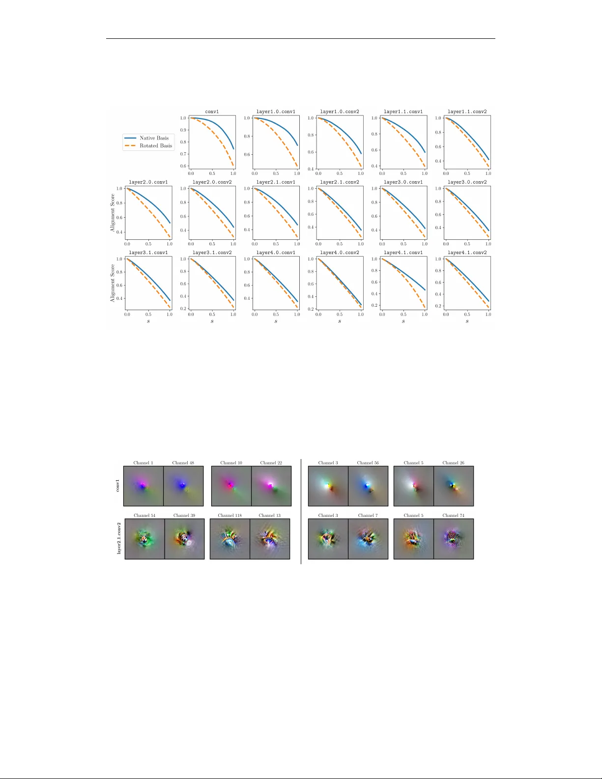
Published as a conference paper at ICLR 2026 P A RT I A L S O F T - M A T C H I N G D I S T A N C E F O R N E U R A L R E P R E S E N T A T I O N A L C O M P A R I S O N W I T H P A RT I A L U N I T C O R R E S P O N D E N C E Chaitanya Kapoor Department of Cognitiv e Science Univ ersity of California, San Diego La Jolla, CA, 92093 chkapoor@ucsd.edu Alex H. Williams Center for Neural Science, New Y ork Univ ersity Center for Computational Neuroscience, Flatiron Institute New Y ork City , NY , 10003 alex.h.williams@nyu.edu Meenakshi Khosla Department of Cognitiv e Science Department of Computer Science and Engineering Univ ersity of California, San Diego La Jolla, CA, 92093 mkhosla@ucsd.edu A B S T R A C T Representational similarity metrics typically force all units to be matched, mak- ing them susceptible to noise and outliers common in neural representations. W e extend the soft-matching distance to a partial optimal transport setting that allows some neurons to remain unmatched, yielding rotation-sensitiv e but ro- bust correspondences. This partial soft-matching distance provides theoretical advantages—relaxing strict mass conservation while maintaining interpretable transport costs—and practical benefits through ef ficient neuron ranking in terms of cross-network alignment without costly iterative recomputation. In simula- tions, it preserves correct matches under outliers and reliably selects the cor- rect model in noise-corrupted identification tasks. On fMRI data, it automati- cally excludes low-reliability vox els and produces vox el rankings by alignment quality that closely match computationally expensi ve brute-force approaches. It achiev es higher alignment precision across homologous brain areas than standard soft-matching, which is forced to match all units reg ardless of quality . In deep networks, highly matched units exhibit similar maximally exciting images, while unmatched units show di ver gent patterns. This ability to partition by match quality enables focused analyses, e.g ., testing whether networks have pri vileged axes ev en within their most aligned subpopulations. Overall, partial soft-matching provides a principled and practical method for representational comparison under partial correspondence. 1 I N T R O D U C T I O N Understanding how design choices ( e.g ., training objectives, architecture) shape neural representa- tions requires comparing how different systems encode information. A fundamental challenge in this comparison is determining which computational units correspond across systems: do specific neurons implement similar functions across networks? This is central to understanding whether different systems con verge to similar computational solutions. Most existing representational sim- ilarity metrics, such as CKA (Kornblith et al., 2019), RSA (Kriegeskorte et al., 2008), Procrustes distance (W illiams et al., 2021; Ding et al., 2021), and CCA variants (Raghu et al., 2017), are rotation-in variant—they measure geometric similarity while ignoring the specific axes along which All code is publicly av ailable at: https://github.com/NeuroML-Lab/partial-metric/ 1 Published as a conference paper at ICLR 2026 information is encoded. This limitation pre vents us from understanding neuron-le vel correspon- dence and whether systems share axis-aligned representations. s partial ( N A , N B ) N A N B N A N B A B Figure 1: Partial Soft-Matching Distance for Matching T uning Curves. (A) T wo toy networks N A and N B ; the layer of interest for alignment is shown in red. A partial matching recov ers one- to-one correspondences between units with highly similar tuning curves. Line color encodes match strength (darker = stronger). By contrast, a purely soft-matching yields a spurious pair (hatched units, red dotted line). (B) The same metric can be used to rank voxel/unit tuning-curve similarity between two subjects’ responses { r 1 , r 2 } , when exposed to the same visual stimulus. T o address these challenges, Khosla & W illiams (2024) recently proposed a metric based on discrete optimal transport (OT ; Peyr ´ e et al., 2019) called the soft-matching distance which finds rotation- sensitiv e correspondences between neurons while remaining in variant to their ordering. Ho wever , this approach requires that all neural units are matched across networks. This requirement may be a crucial limitation in certain settings, since neural populations often contain noisy , inactiv e, or task- irrelev ant units—particularly in biological recordings from fMRI or electrophysiology . Moreo ver , ev en task-relev ant units may be model-specific, implementing computations unique to a particular architecture or training regime in deep neural networks (DNNs). When comparing networks, we should not expect complete o verlap in their functional units. Forcing all units into correspondence may therefore inflate distances and produce misleading alignments. Here, we introduce the partial soft-matching distance (Fig. 1), which allows a fraction of neurons to remain unmatched while preserving robust correspondences among the remainder . Our method provides se veral key adv antages: • Theoretical robustness: Relaxing mass conservation allo ws the metric to handle populations with different numbers of units, where some may lack correspondence ( e .g. , due to noise). • Computational efficiency: Achiev es comparable rankings with a single O ( n 3 log n ) computa- tion, unlike brute-force methods requiring O ( n 4 log n ) operations. • Interpretable partitioning: Separates well-matched from unmatched units, enabling focused analysis of aligned subpopulations. W e demonstrate these advantages through controlled simulations showing correspondence despite spurious neurons, and accurate model identification in noise-corrupted scenarios. In fMRI data from the Natural Scenes Dataset (Allen et al., 2022), our method discards low-quality vox els and outperforms standard soft-matching in aligning homologous brain regions across subjects. When applied to DNNs, we find that highly-matched units produce similar maximally exciting images (MEIs) across models, while unmatched units show di vergent MEIs, suggesting distinct computa- tional roles. Crucially , filtering unmatched units using partial soft-matching improv es alignment ov er heuristics based on soft-matching correlations, matching the performance of a computationally intensiv e brute-force method that iteratively remov es units in a greedy f ashion. This frame work pro- vides a principled approach for comparing neural representations under partial correspondence—a common scenario in neuroscience and AI. 2 Published as a conference paper at ICLR 2026 2 M E T H O D S The optimal transport (O T) problem finds the minimum-cost mapping between probability distrib u- tions, yielding metrics like the soft-matching distance (Khosla & W illiams, 2024). Ho wev er, clas- sical O T requires equal total mass between distributions—a constraint violated in neural recordings where units may be noisy , inacti ve, or genuinely non-corresponding. W e extend the soft-matching distance to handle these realistic scenarios through partial optimal transport. 2 . 1 S O F T - M AT C H I N G D I S TA N C E Consider two neural populations with N x and N y units respecti vely , each with “tuning curves”, { x i } N x i =1 and { y j } N y j =1 taking values in R M . Each unit’ s tuning curv e, respecti vely denoted x i and y j for the tw o neural populations, represents a neuron’ s response ov er a set of M probe stimuli. Stack- ing these tuning curve v ectors column-wise produces matrices X ∈ R M × N x and Y ∈ R M × N y . The soft-matching distance treats each population as a uniform empirical measure and quantifies the optimal transport cost between them: d T ( X , Y ) = min T ∈T ( N x ,N y ) p ⟨ C , T ⟩ F where C ij = ∥ x i − y j ∥ 2 is the squared Euclidean transport cost, ⟨· , ·⟩ F the Frobenius inner product, and T ( N x , N y ) is the transportation polytope (De Loera & Kim, 2013), i.e., the set of all N x × N y nonnegati ve matrices whose ro ws each sum to 1 / N x and whose columns each sum to 1 / N y . This formulation is permutation-in variant yet rotation-sensiti ve, re vealing single-neuron tuning alignment. Furthermore, d T is symmetric and satisfies the triangular inequality , which has been argued to be important for certain analyses of neural representations (W illiams et al., 2021; Lange et al., 2023). The key limitation (which we document in Sections 3 and 4) is that the marginal con- straints (i.e. that the transport plan T lie within the transportation polytope) forces all units to be matched, producing spurious correspondences when populations contain non-corresponding units. 2 . 2 P A RT I A L S O F T - M AT C H I N G D I S TA N C E The soft-matching formulation requires the two empirical distributions to have identical total mass and further enforces that all mass must be transported. The partial OT problem extends this by allowing only a pre-specified fraction 0 ≤ s ≤ 1 of the total mass to be matched at minimal cost. Formally , for empirical measures with unit total mass, a natural set of admissible couplings is T s ( N x , N y ) =    T ∈ R N x × N y +       N y X j =1 T ij ≤ 1 N x , N x X i =1 T ij ≤ 1 N y , X i,j T ij = s    . Here, the inequalities on the row/column marginals permit mass to remain unmatched in either population, and the scalar s controls the total matched mass. Since we normalize our populations to hav e unit total mass, s directly represents the fraction of units that are actually matched. The partial soft-matching distance is then the minimum transport cost ov er this feasible set, d T ( X , Y X ) = min T ∈T s ( N x ,N y ) ⟨ C , T ⟩ F , with C the usual cost matrix ( e.g ., C ij = || x i − y j || 2 ). In our formulation, we use pairwise cosine distance as the cost function. Se veral numerical approaches have been de veloped to solv e partial OT problems (Benamou et al., 2015; Chizat et al., 2018). More recently , Chapel et al. (2020) augmented the cost matrix with dummy (or virtual) points which are assigned large transportation cost. All mass routed to these dummy nodes is effecti vely discarded, which yields an exact partial-matching solution in the augmented formulation. Partial O T distances do not satisfy the triangle inequality and therefore are not proper metrics. Ho w- ev er, they still provide a symmetric notion of dissimilarity in representation and, as we document in Sections 3 and 4, they provide robust and interpretable tool for tuning-lev el comparisons between neural populations with unequal or noisy measurements. 3 Published as a conference paper at ICLR 2026 2 . 3 C H O O S I N G O P T I M A L R E G U L A R I Z A T I O N T o apply partial soft-matching in practice, we must select the hyperparameter 0 ≤ s ≤ 1 which determines how much mass to transport between distrib utions. This is a key challenge when the abundance of outliers and magnitude of noise in the data are unknown a priori . T o address this, we adopt an L-curve heuristic (Cultrera & Callegaro, 2020), inspired by classical regularization methods for ill-posed problems ( e.g ., T ikhonov regularization). The L-curve captures the trade- off between transport distance and regularization strength, with the “elbow” typically indicating a balanced choice between these competing objectiv es. Concretely , we define the two-dimensional parametric curve: f ( s ) = ( ζ ( s ) , ρ ( s )) →  ζ ( s ) = ⟨ T ( s ) , C ⟩ F ρ ( s ) = 1 − s where C is the cost matrix and T ( s ) is the optimal transport plan for a match fraction s ∈ [0 , 1] . W e interpret ρ ( s ) as the regularization strength—smaller s , or con versely larger ρ permits more mass to be left unmatched. The optimal regularization s 0 is identified at the curve’ s point of maximal positiv e curvature (the elbo w), which balances low transport cost against aggressi ve regularization. In our discrete implementation, we sample s uniformly from a sequence { s i } N i =1 and compute the associated transportation costs ζ i = ζ ( s i ) . W e compute the elbow by approximating the second deriv ativ e of the cost curve with respect to the regularization strength ρ ( s ) by the centered second finite difference δ 2 ρ , δ 2 ρ ζ i = ζ i +1 − 2 ζ i + ζ i − 1 for i = 2 , . . . , N − 1 and select the index with maximal positi ve curvature i ⋆ = arg max 2 ≤ i ≤ N − 1 | δ 2 ζ i | , s 0 = s i ⋆ allowing us to analytically select the optimal re gularization s 0 . 2 . 4 P A RT I A L S O F T - M AT C H I N G A S A C O R R E L A T I O N S C O R E Suppose that the tuning curves in two neuron populations X and Y hav e been mean-centered and scaled to unit-norm. Under this normalization, the inner product x ⊤ i y j is identical to the Pearson correlation between neuron i in X and neuron j in Y . Using this, the optimization can now be recast as a maximization of total matched correlation: d corr ( X , Y ) = max T ∈T s ( N x ,N y ) X ij T ij x ⊤ i y j Intuitiv ely , d corr measures the average correlation between paired neurons under the coupling T . W e report d corr for the remainder of the manuscript. W e also report alignment obtained using a squared Euclidean cost function, C ij = || x i − x j || 2 , in Appendix A1.8 and observe identical results. 2 . 5 I N T E R P R E TA T I O N A N D O U T P U T The optimal transport plan T ⋆ provides a soft partial alignment where: • Row sums ∈ [0 , 1 / N x ] : amount of mass transported from each source neuron • Column sums ∈ [0 , 1 / N y ] : amount of mass recei ved by each tar get neuron • T otal transported mass equals s < 1 (the fraction of total mass matched) • Near-zero row/column sums identify ef fectiv ely unmatched units This partitions populations based on participation in the optimal matching, from completely un- matched to maximally participating units. 4 Published as a conference paper at ICLR 2026 3 S I M U L A T I O N S : R O B U S T N E S S T O N O I S E A N D S E L E C T I N G T H E “ C O R R E C T ” M O D E L W e designed controlled simulations to ev aluate whether partial soft-matching (1) maintains accu- rate correspondences despite spurious neurons and (2) correctly identifies which model shares more signal with a reference population. Synthetic neural representation generation is detailed in Ap- pendix A1.3. 3 . 1 R O B U S T N E S S A G A I N S T S P U R I O U S N E U RO N S W e construct two neural populations X and Y , each containing K “signal” neurons matched pair- wise. W e introduce noise by augmenting X with M x random neurons and Y with M y random neurons, where each random neuron is drawn from ε ∼ N (0 , 1) . The resultant populations are thus X ∈ R ( K + M x ) × N and Y ∈ R ( K + M y ) × N , where N is the number of unique stimuli. (a) (b) Figure 2: Comparison of Balanced and Partial Soft-Matching . (a) W e simulate two neural repre- sentations, X and Y , with 120 and 190 neurons respectively . The first 100 neurons represent pure signal , while the rest are pure noise . Red denotes all pure signal neurons in the two representations. (b) The L-curve method selects the optimal mass regularization parameter (= 90 / 190 ≈ 0 . 47) , successfully discarding noisy units. In the (fully balanced) soft-matching distance must match all K + M x neurons to K + M y neu- rons. This forces spurious outlier-to-outlier assignments, which inflate the ov erall transport cost and, consequently , the distance. In contrast, the partial soft-matching distance only transports mass corresponding to K true matches, ignoring the random neurons. As a result, the reco vered transport cost is significantly smaller and reflects the true correspondence between the signal neurons. W e vi- sualize the transport plans for both—soft-matching and partial soft-matching in Fig. 2, and observe that the L-curve heuristic is able to faithfully distinguish between noise and signal units. 3 . 2 C H O O S I N G B E T W E E N T W O M O D E L S Suppose we consider two models: Model A , where Y a shares exactly K correctly matched neurons with X , along with M y additional noisy neurons; and Model B , where Y b (i) does not contain the same signal neurons as X , and (ii) shares fewer correctly matched neurons. Model A is considered “correct” here because it preserves the maximum number of genuine signal correspondences with X —the K matched neurons encode the same computational features as their counterparts in X —plus additional noisy neurons. These extra neurons may reflect measurement noise, inacti ve recording channels, or recording artifacts that are common in real neural data. Model B , in contrast, shares only a subset of X ′ s signal neurons. W e compute the partial soft-matching scores s partial ( X , Y a ) and s partial ( X , Y b ) . Because partial O T can ignore outliers and preserve only the true K matches, the distance, to the “corr ect” model Y a will be significantly smaller—equi valently , the correlation satisfies s partial ( X , Y a ) > s partial ( X , Y b ) , correctly identifying Model A as sharing more signal with X . By contrast, standard soft-matching forces matches for all units (including noise), obscuring signal differences and failing to discriminate Y a from Y b , as shown in Fig. 3. 5 Published as a conference paper at ICLR 2026 (a) (b) Figure 3: Model Selection Using Partial Soft-Matching. W e simulate three synthetic representa- tions to test whether partial soft-matching correctly identifies which of two candidate models— Y a or Y b —shares more signal with a reference population X (100 units). Y a contains all 100 signal units from X plus 60 noise units; Y b contains 100 units, 80 of which match X . The true fraction of shared units is known a priori , marked by a vertical gray line. W ith the L-curve-selected regularization, par- tial soft-matching yields correlation scores s partial ( X , Y a ) = 0 . 715 and s partial ( X , Y b ) = 0 . 645 , correctly fa voring Y a . Standard soft-matching fails, with s sm ( X , Y a ) = 0 . 339 and s sm ( X , Y b ) = 0 . 415 , incorrectly preferring Y b due to forced matching of noise. 4 A P P L I C A T I O N S I N N E U R O S C I E N C E A N D A I 4 . 1 C O M PA R I S O N S O F N E U R A L R E C O R D I N G S A C R O S S S U B J E C T S Figure 4: Aligning V oxel Responses Between Different Subjects in NSD. For each area, we plot the (i) partial soft-matching score at different mass regularization v alues and (ii) the mean noise ceilings of the vox els that were kept at that regularization. The alignment criterion consistently identifies low noise-ceiling v oxels for exclusion. Perfect correspondence of neural populations across subjects is rare—measurement noise, inactive vox els and anatomical variability implies imprecise region boundary definition. V oxels nominally assigned to the same brain area can sample neighboring regions implementing distinct computa- tions. Individual differences in functional organization can further aggra vate distinct computations across subjects. Partial soft-matching addresses these challenges by selectiv ely excluding non- corresponding units from the alignment. 6 Published as a conference paper at ICLR 2026 W e demonstrate this on vox el responses from a subject pair (IDs 1 and 2 ) across six visual ar- eas (V1v , V1d , V2v , V2d , V3v , V3d) from the Natural Scenes Dataset (Allen et al., 2022). Fig. 4 shows how voxel selection quality changes as we vary the mass regularization parameter s from 1 (including all v oxels) to 0 (excluding all voxels). As s decreases and we exclude more vox els, the mean noise ceiling of the retained voxels steadily increases, while the alignment score between these retained voxels also improves. Since noise ceiling measures the reliability of a voxel’ s responses across repeated stimulus presentations, this demonstrates that our method successfully identifies and excludes voxels with poor response replicability . By progressi vely discarding these unreliable measurements, partial soft-matching automatically focuses the alignment on the subset of voxels that provide the most consistent and well-matched signal across subjects. W e perform an identical experiment on a dif ferent NSD subject pair (Appendix A1.2) and observe identical results. 4 . 2 C O M PA R I S O N A G A I N S T B A S E L I N E M E T H O D S Figure 5: Evaluating Methods f or Identifying (Un)matched Neur ons in Deep Networks. W e com- pare three methods for ranking con volutional kernels by alignment between two ResNet- 18 models trained from different random initializations on ImageNet, across early , middle, and late layers. Removing low-alignment units identified by partial soft-matching yields alignment scores nearly identical to those obtained by remo ving kernels ranked least important via brute-force ablations, while correlation-based rankings perform poorly . In this section, we demonstrate the utility of our metric as an efficient tool for rank-ordering neurons by their degree of cross-population alignment. W e compare three approaches—brute-force match- ing, correlation-based ordering and our proposed partial soft-matching method. W e test these methods in two distinct settings: (1) compar- ing con volutional kernels between two ResNet- 18 models trained from different random initializa- tions on ImageNet (Deng et al., 2009), examining early , middle, and late layers (Fig. 5), and (2) aligning voxel responses between human subjects viewing natural images, across six visual areas (V1v , V1d , V2v , V2d , V3v , V3d) from the Natural Scenes Dataset (Fig. 6). Brute-for ce matching provides the ground-truth ranking by exhausti vely testing each neuron’ s contri- bution to alignment. W e fit an optimal soft-matching transformation to the complete representation, then iterativ ely remove each neuron and recompute the entire soft-matching optimization to measure the impact on alignment score. This produces an exact ranking of neurons by their alignment qual- ity . Ho wever , each soft-matching optimization requires O ( n 3 log n ) operations and for n neurons to test, the total complexity is O ( n 4 log n ) , making this approach computationally prohibitive for realistic population sizes. Corr elation-based ordering attempts a computationally cheaper approximation by computing pair- wise Pearson correlations between neurons using the transport plan from a single soft-matching optimization. As sho wn in Figures 5 and 6, this heuristic fails catastrophically—it incorrectly iden- tifies and remov es neurons that are actually crucial for alignment, resulting in dramatically degraded alignment scores. This failure occurs because individual correlation values don’t capture the global optimization structure of the transport problem. P artial soft-matching offers a nuanced tradeoff. T o obtain a complete ranking of all n neurons (matching the output of brute-force), we would still require n separate optimizations at different reg- ularization values, maintaining O ( n 4 log n ) complexity . Howe ver , for the practically relev ant task of identifying the top X % most-aligned or least-aligned neurons—which suffices for most analy- ses in neuroscience and deep learning which require identifying highly-aligned or poorly-aligned subpopulations rather than complete rankings—a single optimization at the appropriate regulariza- tion value  O ( n 3 log n )  provides near-identical results to brute-force ranking. As Figures 5 and 6 demonstrate, when selecting subsets of neurons at various alignment thresholds, our method’ s 7 Published as a conference paper at ICLR 2026 Figure 6: Evaluating Methods for Identifying (Un)matched V oxels in Brain Data. W e ev aluate three methods for ranking voxels by their degree of alignment between a subject pair from NSD across six visual areas. Removing low-alignment v oxels identified by partial soft-matching yields alignment scores nearly identical to those obtained by removing vox els ranked least important via brute-force ablations, while correlation-based rankings perform poorly . selections yield alignment scores nearly matching those from exhausti ve brute-force ranking, while correlation-based selection performs poorly . Full algorithmic details are provided in Appendix A1.4. 4 . 3 M A P P I N G ( D I S ) S I M I L A R B R A I N R E G I O N S A robust similarity metric for neural populations should e xhibit specificity: it must identify when re- sponses come from the same brain area across subjects (true positives) while a voiding false matches between distinct areas (false positives) (Thobani et al., 2025). This specificity is crucial when anatomical boundaries are imprecise and individual v ariability is high. W e ev aluate this specificity by testing whether partial soft-matching correctly aligns homologous visual areas while maintaining separation between distinct areas. Concretely , we select two visual R OIs in a subject pair and then compute a between-subject matching for all vox els of these regions. For each pair of visual regions within and across subjects from the NSD, we compute the precision of voxel assignments—the fraction of matched vox els that truly belong to corresponding regions. T able 1 sho ws these precision scores comparing standard soft-matching (which must match all v ox- els), thresholding using voxel noise ceilings, and partial soft-matching (which can exclude poor correspondences). The optimal regularization parameter for partial soft-matching is chosen via the L-curve heuristic as described in Section 2.3. Across most region pairs, partial soft-matching achieves higher precision than standard soft- matching and thresholding, with particularly striking improv ements for several cross-area compar- isons ( e.g ., V1d + V2v : 0 . 906 → 0 . 971 ). This improv ement stems from the method’ s ability to ex- clude vox els that lack clear correspondence—whether due to boundary uncertainty or measurement noise. By not forcing these ambiguous vox els into the matching, partial soft-matching maintains cleaner separation between distinct regions while preserving strong alignment within homologous areas. 4 . 4 M A X I M A L L Y E X C I T I N G I M A G E S Maximally Exciting Images (MEIs)—synthetic stimuli optimized to maximize individual unit responses—provide an interpretable visualization of what each neuron “looks for” in its input (Erhan 8 Published as a conference paper at ICLR 2026 Brain Region P air SM Precision ( ↑ ) ParSM Precision ( ↑ ) ϵ = 0 . 1 ( ↑ ) ϵ = 0 . 3 ( ↑ ) V1v + V1d 0 . 839 0 . 905 (0 . 76) 0 . 847 (0 . 98) 0 . 855 (0 . 94) V1v + V2v 0 . 677 0 . 680 (0 . 99) 0 . 680 (0 . 96) 0 . 695 (0 . 88) V1v + V2d 0 . 880 0 . 884 (0 . 99) 0 . 884 (0 . 97) 0 . 894 (0 . 91) V1v + V3v 0 . 798 0 . 853 (0 . 97) 0 . 803 (0 . 99) 0 . 815 (0 . 90) V1v + V3d 0 . 882 0 . 890 (0 . 98) 0 . 890 (0 . 97) 0 . 913 (0 . 91) V1d + V2v 0 . 881 0 . 971 (0 . 71) 0 . 889 (0 . 96) 0 . 906 (0 . 89) V1d + V2d 0 . 706 0 . 708 (0 . 99) 0 . 720 (0 . 97) 0 . 727 (0 . 92) V1d + V3v 0 . 879 0 . 881 (0 . 99) 0 . 885 (0 . 97) 0 . 892 (0 . 91) V1d + V3d 0 . 803 0 . 878 (0 . 76) 0 . 818 (0 . 97) 0 . 828 (0 . 92) V2v + V2d 0 . 869 0 . 879 (0 . 98) 0 . 880 (0 . 95) 0 . 896 (0 . 87) V2v + V3v 0 . 651 0 . 661 (0 . 95) 0 . 653 (0 . 95) 0 . 654 (0 . 86) V2v + V3d 0 . 853 0 . 856 (0 . 99) 0 . 867 (0 . 95) 0 . 882 (0 . 87) V2d + V3v 0 . 833 0 . 971 (0 . 42) 0 . 845 (0 . 96) 0 . 863 (0 . 88) V2d + V3d 0 . 638 0 . 643 (0 . 99) 0 . 642 (0 . 96) 0 . 643 (0 . 89) V3v + V3d 0 . 814 0 . 822 (0 . 99) 0 . 828 (0 . 96) 0 . 852 (0 . 88) T able 1: Precision of Cr oss-Subject V oxel Alignment Within and Across V isual Ar eas . Compar- ison of soft-matching (SM), partial soft-matching (ParSM) and noise ceiling thresholding to align vox els between visual regions in an NSD subject pair . Precision measures the fraction of matched vox els belonging to corresponding anatomical re gions (higher = better specificity). W e include the fraction of total voxels that contribute towards computing alignment in parenthesis. The ϵ values denote the noise ceiling threshold belo w which vox els are excluded. ParSM almost always yields higher precision by excluding v oxels that lack clear correspondence. et al., 2009; Pierzchlewicz et al., 2023; W alker et al., 2019; Bashi van et al., 2019). W e synthesize MEIs 1 for unit pairs from two ResNet-18 models trained with different random seeds, sampling from neurons ranked as highly-matched (top 10% of transport mass) versus poorly-matched (bot- tom 10% ) by our metric. Fig. 7 shows striking differences: highly-matched pairs produce nearly identical MEIs, revealing that these units have conv erged on similar feature detectors despite inde- pendent training. In contrast, unmatched pairs yield diver gent MEIs with distinct visual patterns, confirming they lik ely implement dif ferent computations. W e demonstrate this with some additional results in Appendix A1.7. Matc hed Unmatc hed Figure 7: V isualization of (Un)matched Units Using Maximally Exciting Images. W e sho w MEIs for two layers of ResNet- 18 , comparing units classified as matched or unmatched by the partial soft- matching metric. Matched examples are sampled from the top 10% of partial soft-matching scores; unmatched examples are sampled from the bottom 10% . 4 . 5 T E S T I N G F O R P R I V I L E G E D A X E S I N A L I G N E D N E U R A L S U B P O P U L A T I O N S Neural networks could in principle encode information in arbitrarily rotated coordinate systems, yet recent evidence suggests they conv erge on specific “privileged” axes. Networks trained from 1 Appendix A1.5 9 Published as a conference paper at ICLR 2026 different initializations not only share representational geometry but actually align their coordinate systems—with indi vidual neurons implementing similar computations across networks (Khosla & W illiams, 2024; Khosla et al., 2024; Kapoor et al., 2025). This privile ged basis hypothesis suggests that certain directions in activ ation space are preferred, potentially due to architectural constraints, e.g ., axis-aligned nonlinearities (ReLU). W e ask whether this alignment holds when restricted to the best-matched neurons. Using partial soft-matching, we partition increasingly well-matched neurons and test for privile ged axes from the full population down to the strongest matched pairs. Figure 8: Alignment between ResNet-18 models under original and ran- domly rotated coordinate systems, across early , middle and later layers and matched-mass thresholds. Rotation reduces alignment at all thresholds— including among the best-matched units—supporting con ver gence to a shared coordinate system ev en among the most aligned subpopulations. For two ImageNet- trained ResNet- 18 models initialized with different random seeds, we extract representations { X 1 , X 2 } at each con volutional layer . T o test for privileged axes, we apply a random orthogonal transformation Q (sampled uniformly from the Haar mea- sure) to one network’ s representation and measure how this rotation af fects alignment s partial ( X 1 Q , X 2 ) . If neurons were arbitrarily oriented, this rotation would not affect the alignment. Ho wever , if a privileged basis exists, rotating a way from it should decrease alignment. W e test multiple regularization values ( s ) to sample subpopulations of varying alignment quality . Fig. 8 rev eals that alignment consistently decreases under rotation across for all s and depths, with an identical pattern across all con volutional layers (Appendix A1.6). This demonstrates that privileged coordinate systems persist ev en among the most aligned neural subpopulations—the subset we might expect to be most robustly matched. The persistence of this effect suggests that coordinate alignment is not merely a statistical artifact of analyzing many neurons together , but reflects true con ver gence on similar computational solutions at the single-unit lev el. 5 D I S C U S S I O N W e introduced partial soft-matching, extending O T -based representational comparisons to account for partial correspondence between neural populations. This addresses a key limitation of methods that force all units into alignment, which can obscure genuine matches in the presence of noise. Simulations show that the method preserv es true correspondences under noise and selects the correct model in system identification tasks. In fMRI data, it excludes low-reliability vox els and improves alignment precision across homologous brain regions. In deep networks, matched units exhibit shared MEIs, while unmatched units differ qualitatively . In both domains, partial soft-matching provides a more efficient way to order units by alignment quality , closely matching brute-force ablations, requiring only a single optimization at each chosen mass regularization v alue. Some limitations remain. The L-curve heuristic for selecting matched mass performs well empir- ically , but its generality is unclear . W e list some good practices that a practitioner should keep in mind while using the L-curve method in Appendix A1.1. Alternate strategies ( e.g ., area under the alignment-regularization curve)—may of fer more robust summarization across multiple regulariza- tion values. Because partial O T relaxes mass conservation and violates the triangle inequality , it should be understood as a comparative tool rather than a strict metric. Howe ver , we note that re- cent theoretical w ork has de veloped partial W asserstein v ariants that preserve full metric properties, including the triangle inequality (Raghvendra et al., 2024). Future extensions could integrate these formulations for applications requiring strict metric axioms, such as clustering analyses. Although significantly faster than brute-force baselines, the O ( n 3 log n ) cost can limit scalability to v ery lar ge datasets. These considerations aside, this work highlights that meaningful comparison does not re- 10 Published as a conference paper at ICLR 2026 quire complete unit overlap: partial soft-matching enables principled analysis of con vergent and div ergent representational structure across neural systems. R E F E R E N C E S Emily J Allen, Ghislain St-Yv es, Y ihan W u, Jesse L Breedlove, Jacob S Prince, Logan T Dowdle, Matthias Nau, Brad Caron, Franco Pestilli, Ian Charest, et al. A massiv e 7t fmri dataset to bridge cognitiv e neuroscience and artificial intelligence. Natur e neuroscience , 25(1):116–126, 2022. Pouya Bashi van, K ohitij Kar , and James J DiCarlo. Neural population control via deep image synthesis. Science , 364(6439):eaav9436, 2019. Jean-David Benamou, Guillaume Carlier, Marco Cuturi, Luca Nenna, and Gabriel Peyr ´ e. Iterativ e bregman projections for regularized transportation problems. SIAM Journal on Scientific Com- puting , 37(2):A1111–A1138, 2015. Laetitia Chapel, Mokhtar Z Alaya, and Gilles Gasso. Partial optimal tranport with applications on positiv e-unlabeled learning. Advances in Neural Information Pr ocessing Systems , 33:2903–2913, 2020. Lenaic Chizat, Gabriel Peyr ´ e, Bernhard Schmitzer , and Franc ¸ ois-Xavier V ialard. Scaling algorithms for unbalanced optimal transport problems. Mathematics of computation , 87(314):2563–2609, 2018. Alessandro Cultrera and Luca Callegaro. A simple algorithm to find the l-curve corner in the regu- larisation of ill-posed in verse problems. IOP SciNotes , 1(2):025004, 2020. Jes ´ us A De Loera and Edward D Kim. Combinatorics and geometry of transportation polytopes: An update. Discrete geometry and alg ebraic combinatorics , 625:37–76, 2013. Jia Deng, W ei Dong, Richard Socher , Li-Jia Li, Kai Li, and Li Fei-Fei. Imagenet: A large-scale hier- archical image database. In 2009 IEEE Confer ence on Computer V ision and P attern Recognition , pp. 248–255, 2009. doi: 10.1109/CVPR.2009.5206848. Frances Ding, Jean-Stanislas Denain, and Jacob Steinhardt. Grounding representation similarity through statistical testing. In M. Ranzato, A. Beygelzimer , Y . Dauphin, P .S. Liang, and J. W ortman V aughan (eds.), Advances in Neural Information Pr ocessing Systems , v olume 34, pp. 1556–1568. Curran Associates, Inc., 2021. URL https://proceedings.neurips.cc/paper_ files/paper/2021/file/0c0bf917c7942b5a08df71f9da626f97- Paper.pdf . Dumitru Erhan, Y oshua Bengio, Aaron Courville, and Pascal V incent. V isualizing higher-layer features of a deep network. University of Montr eal , 1341(3):1, 2009. Chaitanya Kapoor , Sudhanshu Sriv astav a, and Meenakshi Khosla. Bridging critical gaps in conv er- gent learning: Ho w representational alignment ev olves across layers, training, and distribution shifts. arXiv preprint , 2025. Meenakshi Khosla and Alex H W illiams. Soft matching distance: A metric on neural representations that captures single-neuron tuning. In Pr oceedings of UniReps: the F irst W orkshop on Unifying Repr esentations in Neural Models , pp. 326–341. PMLR, 2024. Meenakshi Khosla, Ale x H W illiams, Josh McDermott, and Nancy Kanwisher . Privileged represen- tational axes in biological and artificial neural networks. bioRxiv , pp. 2024–06, 2024. Simon K ornblith, Mohammad Norouzi, Honglak Lee, and Geoffrey Hinton. Similarity of neural network representations revisited. In International confer ence on machine learning , pp. 3519– 3529. PMlR, 2019. Nikolaus Kriegeskorte, Marieke Mur , and Peter A Bandettini. Representational similarity analysis- connecting the branches of systems neuroscience. F r ontiers in systems neur oscience , 2:249, 2008. 11 Published as a conference paper at ICLR 2026 Richard D Lange, Devin Kwok, Jordan K yle Matelsky , Xinyue W ang, David Rolnick, and K onrad K ording. Deep networks as paths on the manifold of neural representations. In T imothy Doster, T egan Emerson, Henry Kvinge, Nina Miolane, Mathilde Papillon, Bastian Rieck, and Sophia Sanborn (eds.), Pr oceedings of 2nd Annual W orkshop on T opology , Algebra, and Geometry in Machine Learning (T A G-ML) , volume 221 of Proceedings of Machine Learning Resear ch , pp. 102–133. PMLR, 28 Jul 2023. Gabriel Peyr ´ e, Marco Cuturi, et al. Computational optimal transport: W ith applications to data science. F oundations and T r ends® in Machine Learning , 11(5-6):355–607, 2019. Pa wel Pierzchle wicz, K onstantin W illeke, Arne Nix, Pa vithra Elumalai, Kelli Restiv o, T ori Shinn, Cate Nealley , Gabrielle Rodriguez, Saumil Patel, Katrin Franke, et al. Energy guided dif fusion for generating neurally exciting images. Advances in Neural Information Pr ocessing Systems , 36: 32574–32601, 2023. Maithra Raghu, Justin Gilmer , Jason Y osinski, and Jascha Sohl-Dickstein. Svcca: Singular vector canonical correlation analysis for deep learning dynamics and interpretability . Advances in neural information pr ocessing systems , 30, 2017. Sharath Raghvendra, Pouyan Shirzadian, and Kaiyi Zhang. A new robust partial p -wasserstein-based metric for comparing distributions. arXiv pr eprint arXiv:2405.03664 , 2024. Imran Thobani, Javier Sagastuy-Brena, Aran Nayebi, Jacob S Prince, Rosa Cao, and Daniel LK Y amins. Model-brain comparison using inter-animal transforms. In 8th Annual Confer ence on Cognitive Computational Neur oscience , 2025. Edgar Y W alker , Fabian H Sinz, Erick Cobos, T aliah Muhammad, Emmanouil Froudarakis, Paul G Fahe y , Alexander S Ecker , Jacob Reimer, Xaq Pitkow , and Andreas S T olias. Inception loops discov er what excites neurons most using deep predicti ve models. Nature neur oscience , 22(12): 2060–2065, 2019. Alex H W illiams, Erin K unz, Simon K ornblith, and Scott Linderman. Generalized shape metrics on neural representations. Advances in neural information pr ocessing systems , 34:4738–4750, 2021. 12 Published as a conference paper at ICLR 2026 A 1 A P P E N D I X A 1 . 1 B E S T P R AC T I C E S W e treat the L-curve elbow as a practical heuristic for selecting the matched mass s , rather than a formal rule. As with any hyperparameter in machine learning, the L-curve should be treated as a user-dependent choice. The L-curve typically f ails when the cost-regularization curve ( ζ ( s ) , ρ ( s )) is smooth and monotonic. In this regime, the estimated curvature is uniformly small, and any computed “inflection” is likely an artifact of either numerical noise or local smoothness. A common empirical signature of this failure mode is that the algorithm selects an “optimal” regularization s at either of the tail ends of the ( ζ , ρ ) curv e. When this occurs, we suggest a simple diagnostic—one can visually inspect the L- curve and check the magnitude of curvature at the selected point. Howe ver , if the curv ature profile is non-informativ e, one can use alternati ve rank summary statistics such as area under the ( ζ , ρ ) curve. A 1 . 2 C O M PA R I S O N O F N E U R A L R E C O R D I N G S F O R A N A LT E R NAT E S U B J E C T P A I R Figure A1: Aligning V oxel Responses Between Subject IDs 5 and 7 in NSD. W e plot the partial soft-matching alignment score achie ved at dif ferent mass regularization values and the mean noise ceilings of the voxels that were kept at each regularization. For The alignment criterion consistently identifies low noise-ceiling v oxels for exclusion for Subjects 5 and 7 . A 1 . 3 G E N E R AT I O N O F S Y N T H E T I C D AT A For the synthetic experiments in Section 3, we construct two approximately one-to-one matched “neural representations” by linearly mixing a small subset of latent factors with sparse coefficients. W e first generate a factor matrix F ∈ R m × k whose columns denote the responses of k linearly in- dependent factors across m unique stimuli. Each column is dra wn i.i.d from N (0 , 1) , and the matrix is orthogonalized using the Gram-Schmidt procedure. W e then generate a pair of representations 13 Published as a conference paper at ICLR 2026 Z 1 ∈ R m × n and Z 2 ∈ R m × n as sparse linear mixtures of these factors: X 1 = [ X 1 ] ij ∼ N (0 , 1) , X 2 = [ X 2 ] ij ∼ N (0 , 1) M 1 = S ⊙ X 1 , M 2 = S ⊙ X 2 where S ∈ { 0 , 1 } k × n Z 1 = F M 1 , Z 2 = F M 2 where ⊙ denotes the Hadamard (element-wise) product. The binary mask S controls the degree of sparsity . By using the same support mask for both populations, each column of Z 1 and the corre- sponding column of Z 2 depend on the same subset of f actors but with independent mixing weights. Choosing S to be highly sparse makes each “neuron” depend on only one (or a combination) of fac- tors, thereby producing clear , approximately one-to-one correspondences across the tw o populations with the intent of mimicking selectiv e tuning to a small set of features. T o introduce outliers and measurement noise, we augment each population with additional “noise neur ons” . Concretely , we append n ′ 1 and n ′ 2 columns of i.i.d Gaussian noise ε ∼ N (0 , 1) , yielding Z 1 ∈ R m × ( n + n ′ 1 ) and Z 2 ∈ R m × ( n + n ′ 2 ) . A 1 . 4 B A S E L I N E M AT C H I N G A L G O R I T H M S In this section, we describe the baseline matching algorithms used to rank-order the tuning similar- ities as demonstrated in Sec. 4.2. In all cases, we consider a representation pair Z 1 ∈ R m × n 1 and Z 2 ∈ R m × n 2 where m is the number of stimuli and { n 1 , n 2 } are the number of neurons respectiv ely . Brute-For ce Matching. W e construct a greedy baseline for ordering the deletion of neurons based on their soft-matching correlation score. Starting from a complete set of N neurons, we establish a baseline score. At each iteration, we ev aluate, for e very remaining neuron i , the score obtained after removing neuron i and re-fitting the soft-match transform on the reduced representation. W e then remov e the neuron whose deletion produces the largest decrease in the matching distance (equiv- alently , the largest improvement in the alignment score if removal improv es the score), append it to the deletion order, and repeat on the remaining neurons. Thus, in essence, we construct a rank- or dering of neurons in terms of their tuning similarities based on the soft-matching objective. Algorithm 1 Brute-Force Matching 1: R ← { 1 , . . . , N } ▷ set of remaining neuron indices 2: s ← SoftMatch ( Z 1 : ,R , Z 2: ,R ) ▷ baseline score on full set 3: π ← [ ] ▷ initialize deletion ordering 4: while R  = ∅ do 5: for each i ∈ R do 6: R − i ← R \ { i } 7: s i ← SoftMatch  Z 1 : ,R − i , Z 2: ,R − i  ▷ re-fit soft matching without neuron i 8: ∆ i ← s i − s ▷ change in score produced by deleting i 9: end for 10: i ⋆ ← arg min i ∈ R ∆ i ▷ pick neuron whose deletion most decreases score 11: append i ⋆ to the end of list π 12: R ← R \ { i ⋆ } ▷ permanently remov e neuron 13: s ← s i ⋆ ▷ update current score to the one after deletion 14: end while 15: return π ▷ deletion order from least → most matched Correlation-Based Matching. For each fitted soft-matching plan T on a response pair , we per- form a bidirectional correlation-based voxel matching. W e project responses from one represen- tational pair into the others space f Z 1 = Z 1 T and compute the Pearson correlation between the response pair corr ( f Z 1 , Z 2 ) . W e retain the top- k correlated units in Z 2 , where k is determined by the number of units (un)matched using the partial soft-matching distance to maintain consistency during comparison. W e repeat this procedure in the rev erse direction f Z 2 = Z 2 T ⊤ and compute Pearson correlations corr ( Z 1 , e Z 2 ) to find the matched units. 14 Published as a conference paper at ICLR 2026 Algorithm 2 Correlation-Based Matching Forward mapping (r esponse 1 → response 2): 1: f Z 1 ← Z 1 T 2: c 1 → 2 ← corr  e Z 1 , Z 2  3: kept 2 ← argsort ( c 1 → 2 )[: k ] Reverse mapping (r esponse 2 → response 1): 4: f Z 2 ← Z 2 T ⊤ 5: c 2 → 1 ← corr  Z 1 , e Z 2  6: kept 1 ← argsort ( c 2 → 1 )[: k ] Partial Soft-Matching . For a gi ven regularization value s , we fit a partial soft-matching transport plan T ∈ R n 1 × n 2 between a response pair { Z 1 , Z 2 } . W e compute the outgoing mass r i = P i T ij for each source unit and incoming mass c j = P j T ij for each target unit, and retain only those units whose total mass exceeds a small threshold τ , serving as a way to determine the unmatched units. W e repeat this procedure over a grid of re gularization v alues S ← { s 1 , · · · , s k } , yielding “per- s ” sets of kept units K 1 ( s ) and K 2 ( s ) that are matched. Algorithm 3 Partial Soft-Matching 1: S ← { s 1 , · · · , s k } ▷ initialize a list of regularization v alues 2: τ ← 1e-6 ▷ initialize a threshold for transport weight 3: for m ∈ M do 4: T ← Pa rSM ( m reg = s ) ▷ compute optimal transport plan 5: r i ← P n 2 j =1 T ij for i = 1 , . . . , n 1 ▷ outgoing mass per source unit 6: c j ← P n 1 i =1 T ij for j = 1 , . . . , n 2 ▷ incoming mass per target unit 7: K 1 ← { i | r i ≥ τ } 8: K 2 ← { j | c j ≥ τ } 9: retur n K 1 , K 2 10: end for A 1 . 5 S Y N T H E S I S O F M A X I M A L L Y E X C I T I N G I M A G E S Giv en a CNN f : X → R K that maps an input image x ∈ X ⊂ R h × w × c to K class logits, we define a scalar target g ( x ) as the activ ation of the unit of interest ( e.g ., feature-map channel, readout). For con volutional layers, when aligning representations, we ev aluate channels at the center spatial location, motiv ated by evidence that con volutional feature maps are equiv alent up to a circular shift (W illiams et al., 2021; Kapoor et al., 2025). Fixing the center neuron across channels thus allows us to consistently describe representations. W e synthesize one image per channel by solving: x ⋆ = arg max x ∈ X E τ ∼T g ( τ ( x )) − X r λ r R r ( x ) ! where T is a distribution over input transformations ( e.g ., jitter , crop). Each R r ( · ) is a regularizer with weight λ r . In practice, we sample a new τ at each iteration and maximize the objectiv e via gradient ascent at the center pixel of e very channel. W e implement this optimization with the Lucent library 2 using total variation (TV) as the regularizer . Each synthesized image is of shape 224 × 224 × 3 . 2 https://github .com/T omFrederik/lucent/ 15 Published as a conference paper at ICLR 2026 A 1 . 6 P R I V I L E G E D A X E S P E R S I S T S I N A L L K E R N E L S U B P O P U L A T I O N S Figure A2: T esting f or Privileged Coordinate Systems Across Matched Neural Subpopulations. For all con volutional layers in a pair of ImageNet-trained ResNet- 18 models, we show that a privi- leged solution basis persists. A 1 . 7 A D D I T I O N A L R E S U LT S F O R M A T C H E D M A X I M A L LY E X C I T I N G I M A G E S In the following section, we show additional matched MEI pairs for tw o layers in a ResNet- 18 , while still displaying the top 10% and bottom 10% examples in Fig. A3. Matc hed Unmatc hed Figure A3: Additional visualizations of (Un)matched Units Using Maximally Exciting Images. W e sho w additional MEIs for two layers of ResNet- 18 , comparing more pairs of top matched and unmatched units using the partial soft-matching metric. 16 Published as a conference paper at ICLR 2026 A 1 . 8 S E N S I T I V I T Y T O C H O I C E O F C O S T F U N C T I O N For all results demonstrated in Sec. 4.2, we use cosine similarity to rank-order units. In this section, we construct a squared-Euclidean distance cost matrix (i.e.: C ij = || x i − y j || 2 ) to compute the optimal transport plan. In synthetic e xperiments (Fig. A4-A), deep neural networks (Fig. A4-B) and brain data (Fig. A4-C), we find our conclusions remain unaffected by the choice of cost function. For the brain data and DNN alignment plots, we normalize the distances by their maximum v alue such that values can be visualized in the same plot. Figure A4: Partial Soft-Matching Using a Euclidean Cost Function (A) W e visualize the L- curve elbo w computed using a Euclidean cost function ( left ), and the corresponding transport plans ( right ). W e find that the optimal regularization value s and transport plans are identical to that computed using a cosine similarity cost function. (B) Rank-ordering of neurons from 3 layers (early , middle and late) in an ImageNet-trained ResNet- 18 network using a squared Euclidean cost function. Removing units by using the Euclidean distance yields identical trends as using a cosine similarity cost. (C) W e rank-order voxels from a subject pair in NSD using six visual areas by using a squared Euclidean cost function. Ordering vox els using a Euclidean distance cost function also reveals identical trends as using cosine similarity . 17