A Power Market Model with Hypersaclers and Modular Datacenters

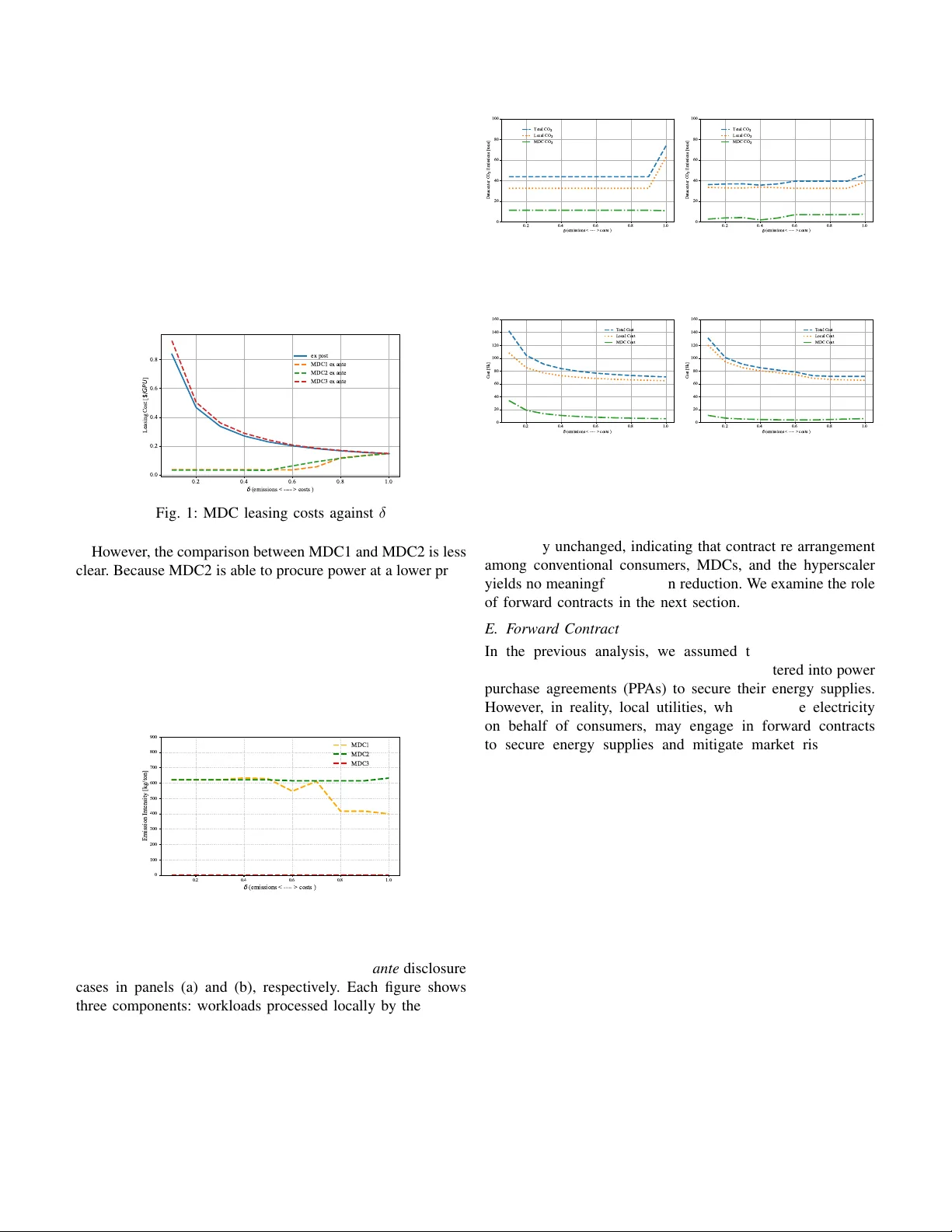
1 A Po wer Market Model with Hypersaclers and Modular Datacenters Y ihsu Chen, Senior Member , IEEE, Abel Souza, Far gol Nematkhah, and Andre w L. Liu Abstract —The rapid adoption of AI has led the gr owth of computational demand, with large language models (LLMs) at the f orefront since ChatGPT’s debut in 2022. Meanwhile, large amounts of renewable energy ha ve been deployed but, ultimately , curtailed due to transmission congestion and inadequate demand. This work develops a power market model that allows hyper - scalers to spatially migrate LLM infer ence workloads to geo- distributed modular datacenters (MDCs), which are co-located with near renewable sources of energy at the edge of the network. W e introduce the optimization problems faced by the h yperscaler and MDCs in addition to consumers, producers, and the electric grid operator , where the hyerscaler enters an agr eement to lease MDCs while ensuring that the requir ed service lev el objectives (SLOs) are met. The overall market model is formulated as a complementarity problem where the proof is provided showing the existence and uniqueness of the solutions. When applying the model to an IEEE RTS-24 bus case study , we show that even with a provision that requir es MDCs to disclose the CO 2 emissions associated with their energy supply sour ces, renting less polluting MDCs is unlikely to yield meaningful emission reductions due to so-called contract-reshuffling . The situation can be mitigated when conv entional loads are supplied by forward contracts through power purchase agreements. This also leads to a decline in system congestion when the hyperscaler becomes increasingly cost-aware. Index T erms —Datacenters, Hyperscalers, Modual Datacenter , Sustainability , Complementarity Problem. I . I N T RO D U C T I O N T HE accelerating adoption of artificial intelligence (AI), led by large language models (LLMs) since the launch of ChatGPT in 2022, has marked the beginning of an era defined by massive and rapidly growing datacenter’ s compu- tational demand. Ho wev er, this rapid expansion comes at the expense of unprecedented increases in ener gy loads. While training LLMs has been widely known as energy-demanding, the energy during the inference phase is often ov erlooked despite processing millions of real-time queries daily . Many U.S. technology firms are securing dedicated energy sources to support the rapid growth of LLM workloads. Notably , Microsoft has partnered with Constellation Energy to restart the Three Mile Island nuclear plant by 2028 [1], while Google is collaborating with Kairos Po wer to deploy 500 MW of small Y . Chen is with the En vironmental Studies Department, the Electrical and Computer Engineering Department, at Univ ersity of California, Santa Cruz, CA, USA (email: yihsuchen@ucsc.edu). A. Souza is with the Computer Science and Engineering Department at Univ ersity of California, Santa Cruz, CA, USA (email: absouza@ucsc.edu). F . Nematkhah is with the Electrical and Computer Engineering Depart- ment at the University of California, Santa Cruz, CA, USA (email: fne- matkh@ucsc.edu). A. Liu is with Edwardson School of Industrial Engineering at Purdue Univ ersity , W est Lafayette, IN, USA (email: andrewliu@purdue.edu). modular reactors between 2030 and 2035 [2]. Howe ver , these long de velopment timelines create a near -term bottleneck, constraining the sustainability and scalability of datacenter operations that remain dependent on fossil-fuel-dominated grids. Data centers are generally categorized into two primary types: hyperscalers and modular data centers (MDCs). Hyper- scalers are highly optimized facilities characterized by lar ge- scale, uniform computing architectures; they typically house hundreds of thousands of serv ers and GPUs [1]. The latter is also known as Edge data centers, i.e., factory built, pre- engineered, and fully tested modular units, ha ving been mostly used by telecommunication companies and mobile operators. It is deli vered on a skid or within a container enclosure instead of traditional on-site construction, and has high bandwidth and low latency network capabilities. Because it is pre-built with standardized and repeatable components, it of fers scalable capacity and rapid deployment. Issues related to the sustainable operation of hyperscale datacenters ha ve receiv ed increasing attention [3]–[11]. For ex- ample, [3] proposed a workload-scheduling algorithm for dat- acenters with on-site rene wables that jointly handles latency- sensitiv e and delay-tolerant workloads while minimizing pro- cessing cost based on electricity prices in the market. Simi- larly , [4] developed a cloud-computing approach that reduces GHG emissions by routing workloads across distributed dat- acenters based on marginal rather than average grid emis- sions, demonstrating the benefit of optimizing w orkloads based on the marginal emission rate. More recently , [5] presented Ecomap, a sustainability-driv en edge computing frame work that dynamically adapts power limits and substitutes with less computing demanding models based on real-time carbon intensity . It demonstrated a 30% reduction in emissions while maintaining latency and efficiency . Similarly , [10] proposed an energy-management framework, DynamoLLM, that lev erages the unique characteristics of LLM inference workloads (e.g., input and output token counts) to reduce energy consumption by dynamically adjusting GPU frequencies while still meeting performance SLOs (Service Lev el Objectives). A common feature of this line of work is that electricity prices and carbon emission rates are treated as exogenous and fixed parameters. In reality , howe ver , large datacenters can materially influence both market prices and marginal emis- sions [9]. That is, both power prices and marginal emission rates are endogenously determined by market supply and demand, affected by datacenter computing loads. Moreo ver , marginal emission rates only reflect infinitesimal changes at the operating mar gin and, therefore, become inappropriate 2 when e valuating load shifts of non-trivial scale. Consequently , cost savings and emission reductions deri ved from marginal- emission-based models may not hold when datacenter loads are significant. One exception is [12], which minimizes CO 2 emissions by subjecting the datacenter operation problem to the optimal conditions of the ISO’ s DC-OPF (Direct-Current Optimal Power Flow) problem. Ho wev er, this implies that the hyperscaler fully anticipates the decisions by the ISO and generators when making their operation decisions, seemingly deviating from market reality . Furthermore, an emer ging but relati vely underexplored strat- egy is to lease distributed MDCs for computing. When strate- gically co-located at the edge of the grid, where renewable generation such as wind or solar is frequently curtailed [13], MDCs can absorb otherwise wasted energy , thereby reducing carbon emissions, alleviating grid congestion, and providing flexible computing capacity that complements hyperscalers [14], [15]. Interest in MDC capacity leasing has gro wn rapidly [6], [16]–[18], with infrastructure pro viders such as EdgeCon- neX, Compass Datacenters, and Schneider Electric offering services that enable hyperscalers to deplo y capacity quickly in geographically strategic locations. Under these arrangements, firms such as Meta, Google, Amazon, and Microsoft lease MDC capacity rather than expanding existing facilities, al- lowing them to accommodate growing inference workloads, reduce latency , improve reliability and geographic redundanc y , and take advantage of local energy conditions, particularly in regions with significant renewable curtailment. Despite these promising dev elopments, the implications of MDC capacity leasing regarding emissions, market inter- actions, and system level impacts remain insufficiently un- derstood, particularly because the development is new . This paper addresses this issue by developing a market model, formulated as a complementarity problem, that considers the decisions faced by con ventional consumers, producers, the grid operator , the hyperscaler , and MDCs. W e assume that power transactions among suppliers, con ventional consumers, the hyperscaler , and MDCs occur through bilateral contracts, allowing the CO 2 footprint associated with workload process- ing to be e xplicitly represented. 1 The hyperscaler allocates workloads between local processing and outsourcing while accounting for both processing costs and the associated CO 2 emissions. MDCs are assumed to be strategically co-located at the edges of the transmission netw ork, allowing them to utilize renew able energy that would otherwise be curtailed in the absence of such facilities. All entities procure electricity through bilateral contracts. Models built on complementarity formulations hav e been previously used to in vestigate interactions among emerging entities, the de velopment of new markets, and the imple- mentation of regulatory or policy interventions in the electric power market [21]. The strength of these models stems from their capacity to explicitly characterize the strategic behavior of multiple agents and to represent their interactions via market-clearing conditions, operational constraints, and equi- 1 In fact, bilateral contracts have also been applied to study California’ s cap-and-trade program [19], and its equiv alence to a pool-based market under perfect competition has been formally established in [20]. librium formulations. Examples include [22] coupled natural- gas and electricity markets to address strategic interactions span multiple infrastructures, [23] examined the interactions between power markets and cap-and-trade systems, and [20] analyzed the Cournot competition among generators under the bilateral and pool-typed electric power market. Finally , [24] showed that while coupling energy storage with rene wables can effecti vely reduce congestion and ramping costs, it may unintentionally increase emissions. Contracts play a piv otal role in power markets, as they en- able both suppliers and loads to hedge against price volatility and other operational risks and hav e been studied extensi vely . For example, [25] developed an iterativ e negotiation scheme that enables suppliers and loads to reach forward power pur- chase agreements while accounting for price uncertainty and heterogeneous risk preferences. More recently , [26] argued that due to moral hazard and adverse selection issues, the current spot markets alone pro vide insufficient incentiv es for zero- carbon in vestment. A contract of a longer duration can mitigate price volatility and facilitate the funding of the in vestments. In this paper , we consider a different type of contracts. That is, the capacity leases between the hyperscaler and MDCs, which indirectly affect energy transactions in the electric power market. This paper explicitly analyzes the capacity leasing contracts between the hyperscaler and the MDCs under two emission-disclosure schemes. Under the ex post scheme, MDCs report their CO 2 emissions only after operations are completed. In contrast, the e x ante scheme requires MDCs to disclose their emission intensities beforehand, enabling the hyperscaler to incorporate these values into its workload allocation decisions. W e hav e the follo wing central findings. First, both ex post and ex ante schemes are unlikely lead to meaningful CO 2 benefits due to contract rearangmenets among conv entional loads, the hyperscalers and MDCs, i.e., contract reshfulling. When con ventional loads are served through forward con- tracts between utilities and suppliers, the extent of contract reshuffling is mitigated, which in turn leads to a reduction in emissions. Second, under the ex ante scheme, the prices of capacity-leasing contracts can dif fer across MDCs when the hyperscaler takes CO 2 emissions into account. In contrast, when processing cost is the sole consideration, all MDCs receiv e the same leasing price despite differences in their emis- sion intensities and in the types of batches they are capable of processing. This highlights the complexity that emerges from the interaction among the hyperscaler’ s objectiv es, the information-disclosure schemes, and the existence of forward contracts in a competitiv e power market. The remainder of the paper is organized as follows. Section II describes the optimization problems faced by each entity in the market. Theoretical properties of the models are analyzed in Section III. The models dev eloped in Section II are then applied to a case study of IEEE 24-bus T est System in Section VI. Numerical simulations are conducted to illustrate our findings. Concluding remarks are summarized in Section V . 3 I I . M O D E L This section presents the optimization problem faced by each entity . The network consists of node i ∈ I . The nodes hosting con ventional loads, the hyperscalers, and the MDCs are, respectiv ely denoted by I d , I κ , and I χ , where the three sets are mutually exclusi ve. That is, I d ∩ I κ = I d ∩ I χ = I κ ∩ I χ = ∅ . A. Conventional Consumer’ s Problem The consumers’ willingness to pay in node i at period t is represented by an affine benefit function B it . The utility in node i procures electricity on behalf of its customers in node i by entering a power purchase agreement (PP A) with producers. Its objectiv e is given in (1) where d j hit denotes the energy sales from the power plant h located in j to i , and where the first and second terms represent the total benefit and the payments, respectiv ely . max d j hit ≥ 0 X t B i  X j,h ∈ H j d j hit  − X j,h ∈ H j ,t θ d j hit d j hit (1) B. Pr oducer’ s Pr oblem Producers solve the profit maximization problem defined in (2) subject to (3), which determines the quantity sold to the utility at node i , denoted by g j hit , subject to the capacity constraint in (3). V ariables θ d j hit , θ χ j hit and θ κ j hit denote the bilateral prices with utilities, the hyperscalers and MDCs, respectiv ely . Note that their values are exogenous to the producers’ problem but endogenous to the overall market equilibrium model. The profits include the first three summations in (2) jointly determine the profit, which equals revenue, minus production cost C j h and the wheeling charge, ω j t . 2 max g j hit ≥ 0 X i ∈ I χ ,t g j hit θ χ j hit + X i ∈ I κ ,t g j hit θ κ j hit + X i ∈ I d ,t g j hit θ d j hit − X j,h ∈ H j ,t C j h  X i g j hit  − X i,j,t ( ω it − ω j t ) g j hit (2) s.t. X i g j hit ≤ G j h ( λ j ht ) (3) C. The Grid Operator The grid operator aims to maximize the value of the trans- mission network by determining the net injection/withdrawal y it where ω it giv es the wheeling charge to bring power from the hub to node i at time t . The grid operator is subject to the energy balance conditions in (5) and to the lower and upper transmission flow limits in (6) and (7), respecti vely , where PTDF refers to the Po wer T ransfer Distribution F actors deriv ed from the linearized DC power flo w model [27]. A similar formulation has been used else-where, e.g., Metzler et al. [28]. max y it free X i,t ω it y it (4) s.t. X i y it = 0 ( γ t ) ∀ t ∈ T (5) 2 For a detailed discussion on wheeling charges, please refer to [20]. − F k − X i ∈ I PTDF ki y it ≤ 0 ( µ 1 kt ) , ∀ k ∈ K, t ∈ T (6) X i ∈ I PTDF ki y it − F k ≤ 0 ( µ 2 kt ) , ∀ k ∈ K, t ∈ T . (7) D. Modular datacenter’s Pr oblem MDCs are assumed to strategically co-locate at the edge of the network where curtailment constantly occurs. The quantities of expected “curtailed” renewables are denoted by P h ∈ H w i g c iht . A MDC maximizes its profits by deciding on power purchase contracts p j hit , leasing contracts with hyperscalers k r bit , and spillov er quantities s it . Note as alluded to earlier, not every MDC can process all the batches; in fact, each MDC has a different latenc y threshold, which can be approximated by the distance between the hyperscaler and MDC [29]. The set of batches that can be processed by the MDCs located in node i is denoted by b ∈ B i , which is determined by the distance between the hyperscaler and the MDCs as well as processing time, which depends on the complexity of the requests characterized by the input and output tokens [30]. The set of variables controlled by the MDCs collectively is denoted as Φ = { p j hit , k r bit , s it } . The maximization problem faced by the MDCs is in (8)– (11). The first term α bit k r bit ν in the objective function Equa- tion (8) describes the re venue from leasing GPUs to the hyperscaler , where α bit is the rev enue from leasing per unit of GPUs, k r bit denotes the leasing capacity , and ν denotes the power rating per GPU. I χ represents the set of nodes with MDCs. The second term represents the power purchase costs, where p j hit and θ χ iht denote the quantity and price of the power purchase agreement with suppliers, respectiv ely . max Φ ≥ 0 X i ∈ I χ ,b,t α bit k r bit ν − X j,h ∈ H j ,t p j hit θ χ j hit (8) s.t. X b k r bit − X j,h ∈ H j p j hit + s it − X h ∈ H ω i g c iht = 0 ( η it ) ∀ i ∈ I χ , t ∈ T (9) X b k r bit − Cap i ≤ 0 ( ρ it ) ∀ i ∈ I χ , t ∈ T (10) s it − X h ∈ H i g c iht ≤ 0 ( υ it ) ∀ i ∈ I χ , t ∈ T (11) The problem is subject to three constraints. Equation (9) imposes energy balance. Equation (10) limits the energy consumed by the migrated batches to be less than or equal to the capacity of the MDCs. Equation (11) requires that the spillov er s it be less than or equal to the amount of curtailed energy . W e next turn to the hyperscaler’ s problem. E. Hyperscale datacenter’ s Problem The hyperscale datacenter’ s problem is given in (12)–(13). The hyperscaler recei ves inference requests, aggregates them into batches q b for b ∈ B , and decides whether to process them locally using ℓ bj hit or to send them to MDCs using k s bit , 4 with decision variables collected in Θ := { ℓ bj hit , k s bit } . The hyperscaler accounts for both processing costs and associated CO 2 emissions, as reflected in the objective (12), where the term weighted by δ captures processing costs and the term weighted by 1 − δ captures CO 2 emissions. Specifi- cally , P b,i ∈ I κ ,t α bit k s bit ν and P b,j,h ∈ H j ,i ∈ I κ ,t ℓ bj hit θ κ ij ht rep- resent local processing and external leasing costs, while P j,h ∈ H j ,i ∈ I χ ,t p j hit e j h and P b,j,h ∈ H j ,i ∈ I κ ,t ℓ bj hit e j h repre- sent local and external CO 2 emissions, respectiv ely . This formulation corresponds to an ex post emission disclosure regime for MDCs. The constraint in (13) ensures that all requests are processed. min Θ ≥ 0 δ   X b,i ∈ I κ ,t α bit k s bit ν + X b,j,h ∈ H j ,i ∈ I κ ,t ℓ bj hit θ κ j hit   +(1 − δ )   X b,j,h ∈ H j ,i ∈ I κ ,t ℓ bj hit e j h + X j,h ∈ H j ,i ′ ∈ I χ ,t p j hi ′ t e j h   (12) s.t. X i ∈ I κ k s bit + X j ∈ I , h ∈ H j , i ∈ I κ ,t ℓ bj hit − q b = 0 ( ψ bt ) ∀ b ∈ B , t ∈ T (13) F . Market Clearing Conditions The following fiv e sets of market clearing conditions, (14)– (17) are included for all j ∈ I , h ∈ H j , and t ∈ T . The first three conditions define the bilateral contract prices between suppliers and (i) consumers, (ii) hyperscalers, and (iii) MDCs. The fourth condition specifies the leasing prices between hyperscalers and MDCs, while the fifth condition determines the wheeling charge. θ d j hit free , d j hit − g j hit = 0 , ∀ i ∈ I d (14) θ χ j hit free , p j hit − g j hit = 0 , ∀ i ∈ I χ (15) θ κ j hit free , X b ℓ bj hit − g j hit = 0 , ∀ i ∈ I κ (16) ω it free , y it = X h ∈ H i ,j ∈ I g ihj t − X j ∈ I ,h ∈ H j g j hit , ∀ i ∈ I (17) α bit free , k s bit − k r bit = 0 , ∀ b ∈ B , i ∈ I κ . (18) G. Equilibrium Models Giv en the problems faced by all the entities are con vex, a necessary and sufficient condition for an optimal solution to satisfy is gi ven by the following first-order or Karush-Kuhn- T ucker (KKT) conditions, one for each variable. Consumers 0 ≤ d j hit ⊥ − B ′ i  X j,h ∈ H j d j hit  + θ d j hit ≥ 0 , ∀ j ∈ I , h ∈ H j , i ∈ I d , t ∈ T . (19) Pr oducers 0 ≤ g j hit ⊥ − X m : { χ,κ,d } θ m j hit + ( ω it − ω j t ) + C ′ j h ( g j hit ) + λ iht ≥ 0 , ∀ j ∈ I , h ∈ H j , i ∈ I , t ∈ T (20) 0 ≤ λ j ht ⊥ G j,h − X i ∈ I g j hit ≥ 0 , ∀ j ∈ I , h ∈ H j , t ∈ T . (21) The Grid Operator For ∀ i ∈ I , t ∈ T : y it free, ω it + X k ∈ K PTDF ki ( µ 1 kt − µ 2 kt ) + γ t = 0 (22) η it free, X i ∈ I y it = 0 (23) For ∀ k ∈ K, t ∈ T : 0 ≤ µ 1 kt ⊥ − F k − X i ∈ I PTDF ki y it ≤ 0 (24) 0 ≤ µ 2 kt ⊥ X i ∈ I PTDF ki y it − F k ≤ 0 (25) Modular datacenter 0 ≤ p j hit ⊥ − θ χ j hit − η it ≤ 0 , ∀ j ∈ I , h ∈ H j , i ∈ I , t ∈ T (26) 0 ≤ k r bit ⊥ α bit ν − η it − ρ it ≤ 0 ∀ b ∈ B , i ∈ I , t ∈ T . (27) For ∀ i ∈ I , t ∈ T : η it free , X b ∈ B k r bit − X j ∈ I ,h ∈ H j p j hit + s it − X h ∈ H ω i g c iht = 0 (28) 0 ≤ ρ it ⊥ X b ∈ B k r bit − Cap i ≤ 0 (29) 0 ≤ s it ⊥ − η it − υ it ≤ 0 (30) 0 ≤ υ it ⊥ s it − X h ∈ H i g c iht ≤ 0 (31) Hyperscalers 0 ≤ κ s bit ⊥ − δ ν α bit − ψ bt ≤ 0 , ∀ b ∈ B , i ∈ I κ , t ∈ T (32) 0 ≤ ℓ bj hit ⊥ − δ θ κ j hit − (1 − δ ) e j h − ψ bt ≤ 0 ∀ b ∈ B , i ∈ I κ , t ∈ T (33) ψ bt free , X i ∈ I κ k s bit + X j ∈ I , h ∈ H j , i ∈ I κ ℓ bj hit − q b = 0 ∀ b ∈ B , t ∈ T (34) The market equilibrium problem is then defined as the col- lection of all KKT conditions (19)–(34), together with the market clearing conditions (14)–(18). The resulting problem can then be solved using complementarity problem solvers such as P A TH [31], Knitro [32], and Gurobi [33]. H. Ex Ante Emission Disclosure Alternativ ely , a hyperscaler may require each MDC to disclose its power purchase agreements along with the corresponding emission intensity . The benefit of doing this a hyperscaler can 5 directly minimize its associated emissions through a capacity leasing agreement. Under this situation, a hyperscaler tends to provide a more competitiv e leasing offer to those MDCs with a lower emissions intensity , leading to a higher α bit . T o study this situation, we modify the aforementioned model by adding a new market clearing condition that cal- culates the MDCs’ emission intensity as follows: ϵ it = P j ∈ I ,h ∈ H j p j hit e j h P j ∈ I ,h ∈ H j p j hit , ∀ i ∈ I x , t ∈ T . (35) W e then replace the first term within the parenthesis preceded by (1 − δ ) in (12) with P j ∈ I χ ϵ it κ s bit . This yields the follo wing condition for k κ bit . 0 ≤ κ s bit ⊥ − δ ν α bit − (1 − δ ) ϵ it − ψ bt ≤ 0 , ∀ b ∈ B , i ∈ I κ , t ∈ T (36) Note it is the term (1 − δ ) ϵ it in (36) that dri ves a wedge, leading to each MDC subject to a dif ferent α bit compared to (32). W e illustrate this observ ation in the numerical case study in Section IV below . I I I . T H E O R E T I C A L A NA LY S I S This section reformulates the equilibrium conditions as a single mixed linear complementarity problem (MLCP), estab- lishes existence, and prov es uniqueness of certain aggregate quantities using monotonicity of the associated operator . A. MLCP F ormulation T o express the MLCP in a compact matrix form, we require explicit functional forms for the consumer benefit functions B i ( · ) in (1) and the power producer cost functions C ih ( · ) in (3). W e hence impose the following standing assumption: Assumption 1 (Affine marginal benefit and mar ginal cost): For each i ∈ I d and t ∈ T , the marginal benefit is affine in the total consumption, B ′ i   X j ∈ I , h ∈ H j d j hit   = b 0 it − X j ∈ I , h ∈ H j b 1 it d j hit , b 1 it ≥ 0 . (37) For each producer ( i, h, t ) , the marginal cost is affine in the bilateral quantity , C ′ j h ( g j hit ) = c 0 j h + c 1 j h g j hit , c 1 j h ≥ 0 . (38) An affine marginal benefit function with b 1 it ≥ 0 implies a concav e quadratic total benefit function and, equiv alently , a downw ard sloping in verse demand function. Empirical evi- dence suggests that aggreg ate electricity demand response to price fluctuations is well-approximated by linear specifications ov er relev ant operating ranges [34]. On the supply side, an affine marginal cost (with c 1 j h ≥ 0 ) implies a con vex quadratic t otal cost function. In po wer system modeling, the heat rate curve of thermal generators, including coal, gas, and oil units, is commonly represented as a quadratic function of output, which directly yields a linear marginal cost. This modeling practice is well documented in classic power system references such as [35]. W e next define the decision vectors used in this formulation. Let the nonnegati ve variable vector be defined as z :=  d, g, λ, µ 1 , µ 2 , p, k r , s, ρ, υ, k s , ℓ  ∈ R n z + , (39) where each block stacks the corresponding components { d j hit } , { g ihj t } , { λ iht } , { µ 1 kt } , { µ 2 kt } , { p j hit } , { k r bit } , { s it } , { ρ it } , { υ it } , { k s bit } , and { ℓ bj hit } , ov er all indices defined in Section II. Similarly , define the vector of free variables as π :=  θ d , θ χ , θ κ , ω , α, y , γ , η , ψ  ∈ R n π , (40) stacking { θ d ihj t } , { θ χ ihj t } , { θ κ ihj t } , { ω it } , { α bit } , { y it } , { γ t } , { η it } , and { ψ bt } . W ith the above notation and Assumption 1, all KKT con- ditions (19) – (34) can be stacked into a compact MLCP in matrix form as follows: 0 ≤ z ⊥ M z + N π + q ≥ 0 , (41a) N ⊤ z = r , (41b) where M ∈ R n z × n z , N ∈ R n z × n π , q ∈ R n z , and r ∈ R n π . T o present the details of the matrices and vectors, we will need additional notations. Define the block diagonal matrix: H d := diag  b 1 it  ⊗ I | I |·| H | , (42) where each ( i, t ) diagonal entry b 1 it is replicated across all ( j, h ) components of d j hit , with b 1 it being the coefficient in the mar ginal benefit function (37). The sign ⊗ denotes the Kronecker product; that is, for generic matrices A ∈ R m × n and B ∈ R p × q , A ⊗ B ∈ R mp × nq is the block matrix whose ( i, j ) th block equals A ij B . Since b 1 it ≥ 0 , it follo ws directly that H d is positiv e semi-definite (PSD). Similarly , define H g := diag  c 1 j h  , (43) with c 1 j h being the coefficient in the marginal cost function (38). H g is also PSD with c 1 j h ≥ 0 . Next, we define a matrix A λ ∈ R |I λ |×|I g | component-wise as follo ws. For any row index ( i, h, t ) ∈ I λ and any column index ( i ′ , h ′ , j ′ , t ′ ) ∈ I g ,  A λ  ( i,h,t ) , ( i ′ ,h ′ ,j ′ ,t ′ ) = ( 1 , if i = i ′ , h = h ′ , t = t ′ , 0 , otherwise , (44) which is referred to as producer generation incidence matrix such that ( A λ g ) iht = P j g ihj t . Then the M matrix in (41a) can be written as M :=   H d 0 0 0 H g A ⊤ λ 0 − A λ 0   , (45) where each zero denotes a block of appropriate dimension filled with zeros. The non-square matrix N in (41a) and (41b) collects the coefficients of the free v ariables π in the complementarity conditions. The vector q collects the constants in the comple- mentarity conditions, while r collects the constant right-hand sides of the linear equality constraints. Their specific forms are provided in Appendix A. 6 B. MLCP Solution Existence A pair ( z ∗ , π ∗ ) satisfying (41a) and (41b) is called a solution of the MLCP and corresponds to a market equilibrium. W e es- tablish existence of such a solution using the matrix properties of (41). T o do so, we need another assumption as follows. Assumption 2 (F easibility to meet batch load): The batch load q b for all b ∈ B can be supplied by available generators without violating their capacity constraints or transmission limits; that is, for the giv en generation capacity G and transmission line capacity F , the set F := { ( ℓ, g , y ) ∈ R n ℓ + × R n g + × R n y | (16) , (17) , (21) , (23) , (24) , (25) , (34) } is nonempty . This assumption can be verified by solving a linear opti- mization problem: fix t ∈ T and define Q t := P b ∈ B q b . Let Λ ∗ t ( G, F ) denote the optimal objective function value of the following linear program, parameterized by ( G, F ) : max g ≥ 0 , y free X j ∈ I X h ∈ H j X i ∈ I κ g j hit s.t. X i ∈ I κ g j hit ≤ G j h , ∀ j ∈ I , h ∈ H j , y it = X h ∈ H i ,j ∈ I g ihj t − X j ∈ I ,h ∈ H j g j hit , ∀ i ∈ I , X i ∈ I y it = 0 , − F k ≤ X i ∈ I PTDF ki y it ≤ F k , ∀ k ∈ K . It is straightforward to verify that F  = ∅ if and only if Q t ≤ Λ ∗ t ( G, F ) . A formal proof is omitted due to space limitations. Theor em 1 (Existence of equilibrium): Under Assumption 1 and 2, the MiCP (41) admits at least one solution ( z ⋆ , π ⋆ ) . Pr oof: W e first establish feasibility of the MLCP; namely , there exist ( z , π ) with z ≥ 0 such that M z + N π + q ≥ 0 and N ⊤ z = r . Fix a t ∈ T , we can construct a feasible point as follows. Choose ( ℓ, g , y ) ∈ F . By definition of F , the gener- ation variables satisfy g j hit = P b ℓ bj hit for all i ∈ I κ , j ∈ I , and h ∈ H j . For all i ∈ I \ I κ , set g j hit = 0 for all j ∈ I and h ∈ H j . For all i ∈ I , define s it := P h ∈ H ω i g c iht . Set the re- maining v ariables ( d, p, k r , k s , ρ, υ , µ 1 , µ 2 , λ, ω , α, ψ , θ κ ) all equal to zero. Under this construction, the equality constraints (14)–(18), (22), and (28) are satisfied, as are the inequality constraints in (29) and (31)–(33). For the remaining inequalities, set θ d = b 0 with matching dimension, where b 0 is the constant appearing in (37). This guarantees the inequality in (19). Next, choose a scalar L > 0 sufficiently large and define θ χ = − L 1 , η = L 1 , where 1 denotes a vector of ones of appropriate dimension. With this choice, the inequalities in (20), (26), (27), and (30) all hold. All remaining constraints follow directly from ( ℓ, g , y ) ∈ F . Hence, the MLCP (41) is feasible. For the matrix M defined in (45), since both H d and H g are PSD, so is M by definition; that is, x ⊤ M x ≥ 0 ∀ x ∈ R n z , where n z is the dimension of M . By Lemma EC.1 in [19], an MLCP of the form (41) is solv able (that is, a solution exists) if it is feasible and the matrix M is PSD. Therefore, the MLCP admits a solution. C. MLCP Solution Uniqueness The preceding results establish the existence of a market equilibrium, which may be not unique in general. This raises the question of whether numerical solutions are meaningful for analysis. Follo wing the approach in [19], [36], we can show uniqueness of quantities in the following result. Theor em 2 (Uniqueness of weighted demand and gener- ation): Under Assumptions 1 and 2, for an y tw o equilibria ( z 1 , π 1 ) and ( z 2 , π 2 ) , we hav e H d d 1 = H d d 2 and H g g 1 = H g g 2 , where H d and H g are defined in (42) and (43). Con- sequently , the aggregate demand D it := P j ∈ I P h ∈ H j d j hit is unique. If, in addition, b 1 it > 0 for all i ∈ I , t ∈ T and c 1 j h > 0 for all j ∈ I , h ∈ H j , then d j hit is unique, and the corresponding bilateral generation g j hit is also unique. Pr oof: Define M s := 1 2 ( M + M ⊤ ) . W ith M giv en in (45), we hav e M s = diag ( H d , H g , 0) . As discussed earlier , both H d and H g are PSD, and hence M s is PSD. Lemma EC.2 in [19] implies that for any two solutions of a feasible MLCP of the form (41) with M s PSD, one has M s z 1 = M s z 2 . Therefore, H d d 1 = H d d 2 and H g g 1 = H g g 2 . If b 1 it > 0 , then H d is positiv e definite on the subspace indexed by ( i, t ) , implying d 1 j hit = d 2 j hit for all ( j, h ) . Similarly , if c 1 j h > 0 , then ( H g g ) 1 = ( H g g ) 2 implies g 1 j hit = g 2 j hit . I V . N U M E R I C A L C A S E S T U DY A. Data, Assumptions, and Scenarios W e apply the IEEE Reliability T est System (R TS 24-Bus) [37] to illustrate the model described in Section II . The system consists of 24 buses, 38 transmission lines, and 17 constant-power loads with a total of 2,850 MW . Our analysis groups 32 generators into 13 generators by combining those with the same marginal cost and located at the same node. 6 hydropo wer units are excluded from the dataset giv en the y are operated at their maximum output of 50MW [38]. W e assume that all generators are owned by a single firm, as the analysis does not focus on market power . T o generalize the results, the transmission limit of each line is reduced to 60% in order to produce non-uniform LMPs (Locational Marginal Prices). The marginal cost of generation is modeled as a linear function of output, parameterized by the coefficient vectors C 0 and C 1 , whose elements c 0 j h and c 1 j h are defined in (38). W e assume a hyperscaler is located at node 24, where three MDCs are situated in nodes 11, 12, and 17. Node 24 is one of the nodes that experiences a lower power price at the baseline. 3 The R TS 24-Bus case is first solved as a least-cost min- imization problem with fix ed nodal load to obtain the dual variables. The dual variables, coupled with an assumed price elasticity of -0.2, are then used to define affine in verse demand function. The estimated price elasticity of demand is consistent with findings from previous studies [40]. W e examine the ability of a hyperscaler to pursue sustain- ability (i.e., lowering CO 2 emissions) by leasing computing 3 In fact, analysis in [39] indicates that energy e xpenditures account for more than 40% of total datacenter operating costs. Hyperscalers owned by major technology companies often collaborate with utilities to secure discounted long-term tarif fs. Recent debates ha ve centered on the extent to which other consumers bear a disproportionate share of the fixed costs induced by the rapid e xpansion of datacenters and the impact on local communities. 7 infrastructure from MDCs. These MDCs are strategically co- located at the edge of the network, where renewable energy is frequently curtailed due to insufficient demand or limited transmission capacity . W e assume that MDC1 can process all fi ve batches, MDC2 can process only batches 1–3, and MDC3 can handle only batches 4 and 5. The endowed “curtailed” rene wables for three MDCs equal to 2, 4, and 5 MWh, respectiv ely . The workload in MW that needs to be processed by the hyperscaler is equal to 75, 42, 51, 48 and 69, all in MW for types 1–5, respectiv ely . All batches collecti vely account for roughly 10% of the baseline loads. Our primary results focus on two scenarios: 1) δ = 0 . 1 refers to the case when the hyperscaler is concerned more about CO 2 emissions, and 2) δ = 0 . 9 refers to the case when the hyperscaler is concerned more about processing costs. For each case, we inv estigate two emission disclosure schemes: ex ante and ex post . W e also examine the impact of the hyperscaler’ s preference, denoted by δ , on CO 2 emissions, processing costs, and leasing costs in Section IV -D. B. Ex P ost Disclosur e W e first discuss the results of “ ex post ” emission disclosure in T able I(a)–III(a) for cost, emissions and emission intensity , re- spectiv ely , with a focus on two cases with δ = 0 . 1 (emissions) and δ = 0 . 9 (costs). Note that in both cases, the hyperscaler processes 74% of workload locally . T able I(a) suggests when the hyperscaler concerns more about emissions ( δ = 0 . 1 ), the operator is willing to pay more (0.913 vs. 0.156 $/GPU, reported in T able III(a) bottom panel) to hav e the workload processed by MDCs since they are powered by curtailed rene wables. The total processing cost under δ = 0 . 9 is equal to $71,983, which is significantly lower than that under δ = 0 . 1 at $150,295. T ABLE I: Results: Processing costs [$] (top) & A verage Procurement cost[$/MWh] (bottom) (a) Ex P ost [$] δ = 0 . 1 δ = 0 . 9 Local 113,031 65,617 MDCs 37,264 6,366 T otal Cost 150,295 71,983 MDC1 58.89 58.89 MDC2 52.91 52.91 MDC3 0.00 0.00 (b) Ex Ante [$] δ = 0 . 1 δ = 0 . 9 Local 124,367 66,188 MDCs 3,636 5,701 T otal Cost 128,023 71,888 MDC1 61.06 58.57 MDC2 55.44 52.31 MDC3 0.00 0.00 T able II(a) summarizes the emissions from three sources: local processing at the hyperscaler , outsourced processing at MDCs, and total system emissions. T o our surprise, when the hyperscaler focuses more on cost (i.e., δ = 0 . 9 ), its operation can actually also result in a lo wer level of emissions from outsourcing workloads to MDCs while emissions with the hyperscaler is almost equal. The workload-related CO 2 footprint under δ = 0 . 9 is reduced by 3.56 t (= 39.59–43.15), or approximately 8%. This is because ex post scheme is not a good instrument and thus pro vides an imperfect single to guide the hyperscaler operator to lo wer emissions as it cannot distin- guish MDCs with different emission intensities. Interestingly , ov erall system emissions do not alter between these two cases, suggesting that the decline in MDCs emissions is offset by an increase in emissions associated power sales of con ventional loads. This observ ation is dubbed contract reshuffling. W e illustrate how this can be mitigated in subsection IV -D. T ABLE II: Results: Emissions [t] (a) Ex P ost δ = 0 . 1 δ = 0 . 9 Local 32.51 32.51 MDCs 10.64 7.08 T otal 43.15 39.59 System 1,362.76 1,362.76 (b) Ex Ante δ = 0 . 1 δ = 0 . 9 Local 34.50 32.51 MDCs 1.40 6.46 T otal 35.90 38.97 System 1,361.50 1,370.41 T able III(a) also reports the emission intensity by MDCs. Except MDC3, which has an intensity of 0 kg/MWh as it is powered only by renewables, the other tw o MDCs enter po wer purchase agreements with suppliers. The fact that emissions are disclosed ex post means that the hyperscaler does not hav e information to price GPU leasing dif ferently based on emission intensity and thus leads to the same leasing offer for each MDC. T ABLE III: Results: Emission rate [kg/MWh] (top) & leasing cost [$/GPU] (bottom) (a) Ex P ost δ = 0 . 1 δ = 0 . 9 MDC1 621.0 621.0.0 MDC2 739.0 145.0 MDC3 0.0 0.0 MDC1 0.913 0.156 MDC2 0.913 0.156 MDC3 0.913 0.156 (b) Ex Ante [kg/MWh] δ = 0 . 1 δ = 0 . 9 MDC1 621.1 559.1 MDC2 621.0 145.0 MDC3 0.00 0.00 MDC1 0.036 0.127 MDC2 0.033 0.152 MDC3 0.930 0.157 C. Ex Ante Disclosure The workload processing costs under the ex ante scheme are reported in T able I(b). The hyperscaler maintains total costs at $71,888 under δ = 0 . 9 , comparable to the ex post case ($71,983). In contrast, when δ = 0 . 1 , ov erall workload costs decrease by 34%, from $150,295 in T able I(a) to $128,023 in T able I(b). Under ex ante disclosure, the hyperscaler observes MDC emission intensities and therefore values MDC capacity leasing less as δ increases and as emission intensity rises (see Section IV -D). For example, when emission intensity is 0 t/MWh, T able III(b) shows that the hyperscaler is willing to pay $0.930/GPU for MDC3 at δ = 0 . 1 , compared to $0.157/GPU at δ = 0 . 9 . A similar pattern appears under the ex post scheme, although interpretation is complicated because emission profiles are not distinguished. For a given δ , lo wer MDC emission intensity leads to higher capacity leasing prices under ex ante disclosure. Consistent with this, MDC1 and MDC2 command higher leasing prices under δ = 0 . 9 than under δ = 0 . 1 , for example $0.127 versus $0.036 for MDC1 and $0.152 versus $0.033 for MDC2. This dif ferentiation does not arise under e x post disclosure. Despite these pricing effects, ov erall system emissions in T able II(b) remain comparable to those in T able II(a), indicating that ex ante disclosure alone does not yield meaningful sustainability gains. D. Sensitivity Analysis Figure 1 shows the leasing costs of the three MDCs as a function of δ . The solid blue denotes the ex post scheme while 8 the color -coded dashed lines represent the e x ante scheme for three MDCs. Under the ex post scheme, the hyperscaler is only aw are of CO 2 after the fact. Thus, its willingness to pay for outsourcing workload is the same for all three MDCs. Howe ver , when the hyperscaler becomes aware of the respectiv e emission impact of each MDC under the ex ante scheme before the fact, as allude to earlier , the operator’ s willingness to pay for the services then also depends on the emission intensity of each MDC in Fig. 2. Giv en MDC3 has no emission, the capacity leasing cost curve of MDC3 lies abov e the other tw o MDCs until the δ approaches 1 where the processing cost is the only concern. 0.2 0.4 0.6 0.8 1.0 ( e m i s s i o n s < - - - - > c o s t s ) 0.0 0.2 0.4 0.6 0.8 L e a s i n g C o s t [ $ / G P U ] ex post MDC1 ex ante MDC2 ex ante MDC3 ex ante Fig. 1: MDC leasing costs against δ Howe ver , the comparison between MDC1 and MDC2 is less clear . Because MDC2 is able to procure power at a lower price by an av erage of 6$/MWh across the scenarios, the owner is willing to operate the facility at a lower capacity leasing price (for δ between 0.5 and 0.7) while still maintaining its profit margin ev en though its emission intensity is lower as alluded to in Fig. 2. Overall, as δ approaches 1, emission intensity is no longer a concern for the hyperscaler, ev entually leading to identical leasing prices for all MDCs. 0.2 0.4 0.6 0.8 1.0 ( e m i s s i o n s < - - - - > c o s t s ) 0 100 200 300 400 500 600 700 800 900 Emission Intensity [kg/ton] MDC1 MDC2 MDC3 Fig. 2: MDC CO 2 emission rate against δ Figures 3–4 present datacenter workload related processing costs and CO 2 emissions for the ex post and ex ante disclosure cases in panels (a) and (b), respectively . Each figure sho ws three components: workloads processed locally by the hyper- scaler (red dashed line), workloads outsourced to MDCs (green dashed line), and total quantities (blue dashed line). In both disclosure regimes, increasing δ shifts the datacenter toward cost minimization, resulting in lower local and total processing costs, as shown in Fig. 4. At the same time, CO 2 emissions rise and e ventually spike as δ approaches 1, as shown in Fig. 3, when processing cost becomes the dominant objectiv e. Collectiv ely , these figures illustrate a trade off between CO 2 (a) ex post 0.2 0.4 0.6 0.8 1.0 ( e m i s s i o n s < - - - - > c o s t s ) 0 20 40 60 80 100 D a t a c e n t e r C O 2 E m i s s i o n s [ t o n s ] T o t a l C O 2 L o c a l C O 2 M D C C O 2 (b) ex ante 0.2 0.4 0.6 0.8 1.0 ( e m i s s i o n s < - - - - > c o s t s ) 0 20 40 60 80 100 D a t a c e n t e r C O 2 E m i s s i o n s [ t o n s ] T o t a l C O 2 L o c a l C O 2 M D C C O 2 Fig. 3: datacenters workload CO 2 emissions against δ (a) ex post 0.2 0.4 0.6 0.8 1.0 ( e m i s s i o n s < - - - - > c o s t s ) 0 20 40 60 80 100 120 140 160 Cost [$k] T otal Cost Local Cost MDC Cost (b) ex ante 0.2 0.4 0.6 0.8 1.0 ( e m i s s i o n s < - - - - > c o s t s ) 0 20 40 60 80 100 120 140 160 Cost [$k] T otal Cost Local Cost MDC Cost Fig. 4: datacenters workload processing costs against δ emissions and total processing costs. Across all cases under both schemes, howe ver , total system CO 2 emissions remain essentially unchanged, indicating that contract re arrangement among con ventional consumers, MDCs, and the hyperscaler yields no meaningful emission reduction. W e examine the role of forward contracts in the next section. E. F orwar d Contract In the pre vious analysis, we assumed that consumers, the hyperscaler , and the MDCs simultaneously entered into power purchase agreements (PP As) to secure their energy supplies. Howe ver , in reality , local utilities, which procure electricity on behalf of consumers, may engage in forward contracts to secure energy supplies and mitigate market risk. These arrangements limit the extent to which datacenters, i.e., hy- perscalers and MDCs, can claim renewable energy benefits. T o examine this, the analysis sets a lo wer bound of g ihj t , ranging from 60%–90%, defined by the baseline at which the processing loads of datacenters equal zero. In other words, this represents the bilateral contract position of conv entional loads in the absence of datacenters. The higher the bound is, the more limited that the datacenter can explore contracts to minimize its CO 2 footprint. Figure 5(a) plots total system CO 2 emissions as a function of δ under forward contract requirements ranging from 60% to 90% in the ex ante scheme. The solid black line indicates the maximum system-wide emissions of 1,370 t. For contract positions below 90%, emission reductions are achiev able for δ ≤ 0 . 6 , depending on the hyperscaler’ s concern for CO 2 reductions. The magnitude of this reduction is in versely related to the forward contract position. When the forward contract requirement is set at 90%, leaving only 10% procurement flex- ibility for datacenters, the system exhibits a modest emission reduction of 2–5% relati ve to the baseline. This highlights that contract re-shuf fling can be mitigated by forward contracts. Figure 5(b) displays the results on network congestion. The 9 (a) CO 2 emission 0.2 0.4 0.6 0.8 1.0 ( e m i s s i o n s < - - - - > c o s t s ) 1280 1300 1320 1340 1360 1380 1400 S y s t e m C O 2 [ t o n s ] 90% 80% 60% 70% (b) Congestion 0.2 0.4 0.6 0.8 1.0 ( e m i s s i o n s < - - - - > c o s t s ) 0 100 200 300 400 500 600 System congestion cost [$k] 90% 80% 60% 70% Fig. 5: T otal system CO 2 emissions and congestion cost against δ under different forward contract positions for the ex ante scheme solutions show that under 60%-80% forward contract cases, there is little impact on the system congestion because of the occurence of contract re-shuffling. Howe ver , under 90% case, as the hypercaler becomes more cost-aw are (to ward the right), it allocates more workload to the MDCs in order to lowering processing costs, leading to a decline of the system congestion. V . C O N C L U S I O N S Since the debut of ChatGPT in 2022, issues related to sus- tainable operation of datacenters, including hyperscalers and MDCs, hav e been at the forefront of debates. This paper stud- ies the capacity leasing contract between the hyperscaler and MDCs by developing a power market model, formulated as complementarity problems considering the optimizations faced by con ventional consumers, producers, the grid operator, the hyperscaler and MDCs. W e consider two emission disclosure schemes. Under the e x post scheme, MDCs report their CO 2 emissions after the fact, whereas the ex ante scheme enables the hyperscaler to ev aluate the emissions implications of its workload allocation decisions based on each MDC’ s reported carbon intensity in PP As. W e show that the ex ante scheme can, in principle, re- duce CO 2 emissions by pricing the capacity leasing contract according to the MDCs’ emission intensities. Ho wever , this benefit is unlikely to materialize in practice due to contract reallocation among market participants. W e further demon- strate that moderate emission reductions are possible in our application to the R TS-24 system when conv entional loads are subject to forward contract requirements. This highlights that claims of ”100% rene wable-po wered” datacenters may be misleading unless they correspond to verifiable, short-run emission reductions or are supported by ne wly de veloped renew able resources dedicated to the operations of datacenters. Our analysis is subject to several limitations. First, we assume that all batches yield the same revenue regardless of latency requirements. In practice, some inferences are more time sensitiv e, such as those requested by users subscribed to higher tier services, and therefore generate higher v alue. In this case, an MDC capable of processing a wider range of batches could generate greater re venue for the hyperscaler, leading the hyperscaler to offer higher capacity leasing prices and resulting in differential pricing outcomes. Second, we assume that the amount of rene wable energy that would otherwise be curtailed is fixed. In practice, capacity leasing prices may depend on the hyperscaler’ s expectations of future curtailment lev els, which would require a stochastic framew ork to capture this uncertainty . W e leav e these extensions to future work. A P P E N D I X A T H E M L C P F O R M U L A T I O N – A D D I T I O NA L D E TA I L S The matrix N in (41) collects the coef ficients of the free variables π in the KKT conditions. Consistent with the ordering of the variables in z and π defined in (39) and (40), the nonzero block rows of N π are ( N π ) d = E d θ d , ( N π ) g = − E d g θ d − E χ g θ χ − E κ g θ κ + A ω ω , ( N π ) µ 1 = A µy y , ( N π ) µ 2 = − A µy y , ( N π ) p = E χ p θ χ + E pη η , ( N π ) k r = E kr η η − ν E kr α α, ( N π ) s = E sη η , ( N π ) k s = δ ν E ksα α + E ksψ ψ , ( N π ) ℓ = δ E ℓθ θ κ + E ℓψ ψ . Here each E • is a matrix with entries in { 0 , 1 } to ensure dimensional consistency of the matrix–vector products. The matrix A ω encodes ( ω it − ω j t ) in the g -stationarity rows, and ( A µy y ) kt = P i ∈ I PTDF ki y it . All remaining block rows are zero. The constant vector q in (41) collects the constant terms in the KKT inequality constraints. Its nonzero blocks are q d = −  b 0 , q g =  C 0 , q λ =  G , q µ 1 =  F , q µ 2 =  F , q ρ =  Cap , q υ =  g c , and q ℓ = (1 − δ )  e , where each arrow denotes the vector obtained by stacking and replicating the corresponding parameter to match the dimension of the associated block of z . All remaining blocks of q are zero. The vector r in (41) collects the right-hand sides of the equality constraints whose multipliers are free variables. The only nonzero blocks are r η =  g c and r ψ =  q B , where  q B stacks { q b } and is replicated o ver t . All remaining components of r are zero. R E F E R E N C E S [1] N. Jones, “How to stop data centres from gobbling up the world’ s electricity , ” Natur e , vol. 621, pp. 670–673, 2018. [2] M. T errell, “Ne w nuclear clean energy agreement with Kairos Po wer, ” blog.google/outreach- initiatives/sustainability/ google- kairos- power - nuclear- energy- agreement/. [3] H. Dou, Y . Qi, W . W ei, and H. Song, “Carbon-aware electricity cost minimization for sustainable data centers, ” IEEE T ransactions on Sus- tainable Computing , vol. 2, no. 2, pp. 211–223, 2017. [4] T . Dandres, R. Farrahi Moghaddam, K. K. Nguyen, Y . Lemieux, R. Samson, and M. Cheriet, “Consideration of marginal electricity in real-time minimization of distrib uted data centre emissions, ” Journal of Cleaner Pr oduction , vol. 143, pp. 116–124, 2017. [5] V . Paramanayakam, A. Karatzas, D. Stamoulis, and I. Anagnostopoulos, “Ecomap: Sustainability-driv en optimization of multi-tenant dnn ex ecu- tion on edge servers, ” IEEE T ransactions on Computers , vol. 74, no. 11, pp. 3925–3937, 2025. [6] I. Goiri, W . Katsak, K. Le, T . D. Nguyen, and R. Bianchini, “Parasol and greenswitch: managing datacenters powered by renewable energy , ” in Pr oceedings of the Eighteenth International Confer ence on Arc hi- tectural Support for Progr amming Languages and Operating Systems , ser . ASPLOS 13. New Y ork, NY , USA: Association for Computing Machinery , 2013, pp. 51–64. [7] Z. Liu, Y . Chen, C. Bash, A. W ierman, D. Gmach, Z. W ang, M. Marwah, and C. Hyser , “Rene wable and cooling aware workload management for sustainable data centers, ” ser. SIGMETRICS ’12. Ne w Y ork, NY , USA: Association for Computing Machinery , 2012, p. 175–186. [8] S. Naganandhini, C. Sundar, R. Sathya, and G. V enkatesan, “T owards energy-ef ficient data centres: A comprehensive analysis of cooling strategies for maximizing efficiency and sustainability , ” in 2023 Intel- ligent Computing and Contr ol for Engineering and Business Systems (ICCEBS) , 2023, pp. 1–6. [9] J. Dodge, T . Prewitt, R. T achet des Combes, E. Odmark, R. Schwartz, E. Strubell, A. S. Luccioni, N. A. Smith, N. DeCario, and W . Buchanan, 10 “Measuring the carbon intensity of ai in cloud instances, ” in Proceed- ings of the 2022 ACM Conference on F airness, Accountability , and T ranspar ency , ser . F AccT ’22. New Y ork, NY , USA: Association for Computing Machinery , 2022, p. 1877–1894. [10] J. Stojkovic, C. Zhang, I. n. Goiri, J. T orrellas, and E. Choukse, “Dynamollm: Designing llm inference clusters for performance and energy efficienc y , ” in 2025 IEEE International Symposium on High P erformance Computer Ar chitecture (HPCA) , 2025, pp. 1348–1362. [11] I. Hasan, Y . Sang, D. Irwin, and G. Zakeri, “Optimal data center load scheduling in power system operation, ” in 2025 57th North American P ower Symposium (N APS) , 2025, pp. 1–6. [12] J. Lindberg, B. C. Lesieutre, and L. A. Roald, “Using geographic load shifting to reduce carbon emissions, ” Electric P ower Systems Resear ch , vol. 212, p. 108586, 2022. [13] SFGA TE, “California has a huge solar power problem. a fix is coming, ” https://shorturl.at/yuRCl. [14] K. Kim, F . Y ang, V . M. Zav ala, and A. A. Chien, “Data centers as dispatchable loads to harness stranded power , ” IEEE Tr ansactions on Sustainable Ener gy , vol. 8, no. 1, pp. 208–218, 2017. [15] F . Y ang and A. A. Chien, “Large-scale and extreme-scale computing with stranded green power: Opportunities and costs, ” IEEE T ransactions on P arallel and Distributed Systems , vol. 29, no. 5, pp. 1103–1116, 2017. [16] A. A. Chien, R. W olski, and F . Y ang, “The zero-carbon cloud: High- value, dispatchable demand for rene wable power generators, ” The Elec- tricity J ournal , vol. 28, no. 8, pp. 110–118, 2015. [17] Facebook, “Facebook’ s U.S. rene wable energy impact study, ” https://www .rti.org/publication/facebook-u-rene wable-ener gy-impact- study/fulltext.pdf, last opened: 2025. [18] Microsoft, “Modular Datacenter overvie w, ” https://learn.microsoft.com/en-us/previous-v ersions/azure/mdc/mdc- overvie w , last opened: 2025. [19] Y . Chen, A. L. Liu, and B. F . Hobbs, “Economic and emissions im- plications of load-based, source-based, and first-seller emissions trading programs under California AB32, ” Oper ations Researc h , vol. 59, no. 3, pp. 696–712, 2011. [20] B. Hobbs, “Linear complementarity models of Nash-Cournot compe- tition in bilateral and poolco po wer markets, ” IEEE T ransactions on P ower Systems , v ol. 16, no. 2, pp. 194–202, 2001. [21] S. A. Gabriel, A. J. Conejo, J. D. Fuller , B. F . Hobbs, and C. Ruiz, Complementarity Modeling in Energy Markets , ser . International Series in Operations Research & Management Science. New Y ork, NY : Springer , 2012, vol. 180. [22] S. Chen, A. J. Conejo, R. Sioshansi, and Z. W ei, “Equilibria in electricity and natural gas markets with strategic offers and bids, ” IEEE T ransactions on P ower Systems , vol. 35, no. 3, pp. 1956–1966, 2020. [23] Y . Chen and B. Hobbs, “ An oligopolistic power market model with tradable NOx permits, ” IEEE T ransactions on P ower Systems , vol. 20, no. 1, pp. 119–129, 2005. [24] V . V irasjoki, P . Rocha, A. S. Siddiqui, and A. Salo, “Market impacts of energy storage in a transmission-constrained po wer system, ” IEEE T ransactions on P ower Systems , vol. 31, no. 5, pp. 4108–4117, 2016. [25] S. El Khatib and F . D. Galiana, “Negotiating bilateral contracts in electricity markets, ” IEEE T ransactions on P ower Systems , vol. 22, no. 2, pp. 553–562, 2007. [26] N. Fabra and G. Llobet, “Designing contracts for the energy transition, ” International Journal of Industrial Organization , vol. 102, p. 103173, 2025, 51st Annual Conference of European Association for Research in Industrial Economics, Amsterdam, 2024. [27] F . C. Schweppe, M. C. Caramanis, R. D. T abors, and R. E. Bohn, Spot Pricing of Electricity . Boston, MA: Springer, 1988, reprinted 2013. [28] C. Metzler, B. F . Hobbs, and J.-S. Pang, “Nash–Cournot equilibria in power markets on a linearized DC network with arbitrage: Formulations and properties, ” Networks and Spatial Economics , vol. 3, no. 2, pp. 123– 150, 2003. [29] R. Goonatilake and R. Bachnak, “Modeling latency in a network distribution, ” Netw . Commun. T echnol. , vol. 1, pp. 1–11, 2012. [Online]. A vailable: https://api.semanticscholar .org/CorpusID:27211784 [30] G. Wilkins, S. Kesha v , and R. Mortier, “Offline ener gy-optimal llm serv- ing: W orkload-based energy models for llm inference on heterogeneous systems, ” SIGENERGY Ener gy Inform. Rev . , vol. 4, no. 5, p. 113–119, Apr . 2025. [31] M. C. Ferris and T . S. Munson, “Complementarity problems in gams and the path solver1, ” Journal of Economic Dynamics and Contr ol , v ol. 24, no. 2, pp. 165–188, 2000. [32] Artelys, “Knitro: The most advanced solver for nonlinear optimization, ” https://www .artelys.com/solvers/knitro/, last opened: 2025. [33] Gurobi, “Gurobi 13.0: Decision intelligence for enterprises, ” https: //www .gurobi.com/, last opened: 2025. [34] L. Hirth, T . M. Khanna, and O. Ruhnau, “How aggregate electricity demand responds to hourly wholesale price fluctuations, ” Energy Eco- nomics , v ol. 135, p. 107652, 2024. [35] A. J. W ood, B. F . W ollenberg, and G. B. Shebl ´ e, P ower generation, operation, and contr ol . John wiley & sons, 2013. [36] Y . Chen and A. L. Liu, “Emissions trading, point-of-regulation and facility siting choices in the electric markets, ” Journal of Regulatory Economics , v ol. 44, no. 3, pp. 251–286, 2013. [37] C. Grigg, P . W ong, P . Albrecht, R. Allan, M. Bhavaraju, R. Billinton, Q. Chen, C. Fong, S. Haddad, S. Kurug anty , W . Li, R. Mukerji, D. Patton, N. Rau, D. Reppen, A. Schneider, M. Shahidehpour , and C. Singh, “The IEEE Reliability T est System-1996. A report prepared by the reliability test system task force of the application of probability methods subcommittee, ” IEEE T ransactions on P ower Systems , vol. 14, no. 3, pp. 1010–1020, 1999. [38] J. W ang, N. Redondo, and F . Galiana, “Demand-side reserve offers in joint energy/reserve electricity markets, ” IEEE T ransactions on P ower Systems , v ol. 18, no. 4, pp. 1300–1306, 2003. [39] A. Peskoe and E. Martin, “Extracting profits from the public: Ho w utility ratepayers are paying for big tech’s power , ” Harvard Electricity Law Initiativ e, 2025. [40] I. M. L. Aze vedo, M. G. Morgan, and L. Lave, “Residential and regional electricity consumption in the U.S. and eu: How much will higher prices reduce CO2 emissions?” The Electricity Journal , v ol. 24, no. 1, pp. 21– 29, 2011.