Incremental Learning of Sparse Attention Patterns in Transformers

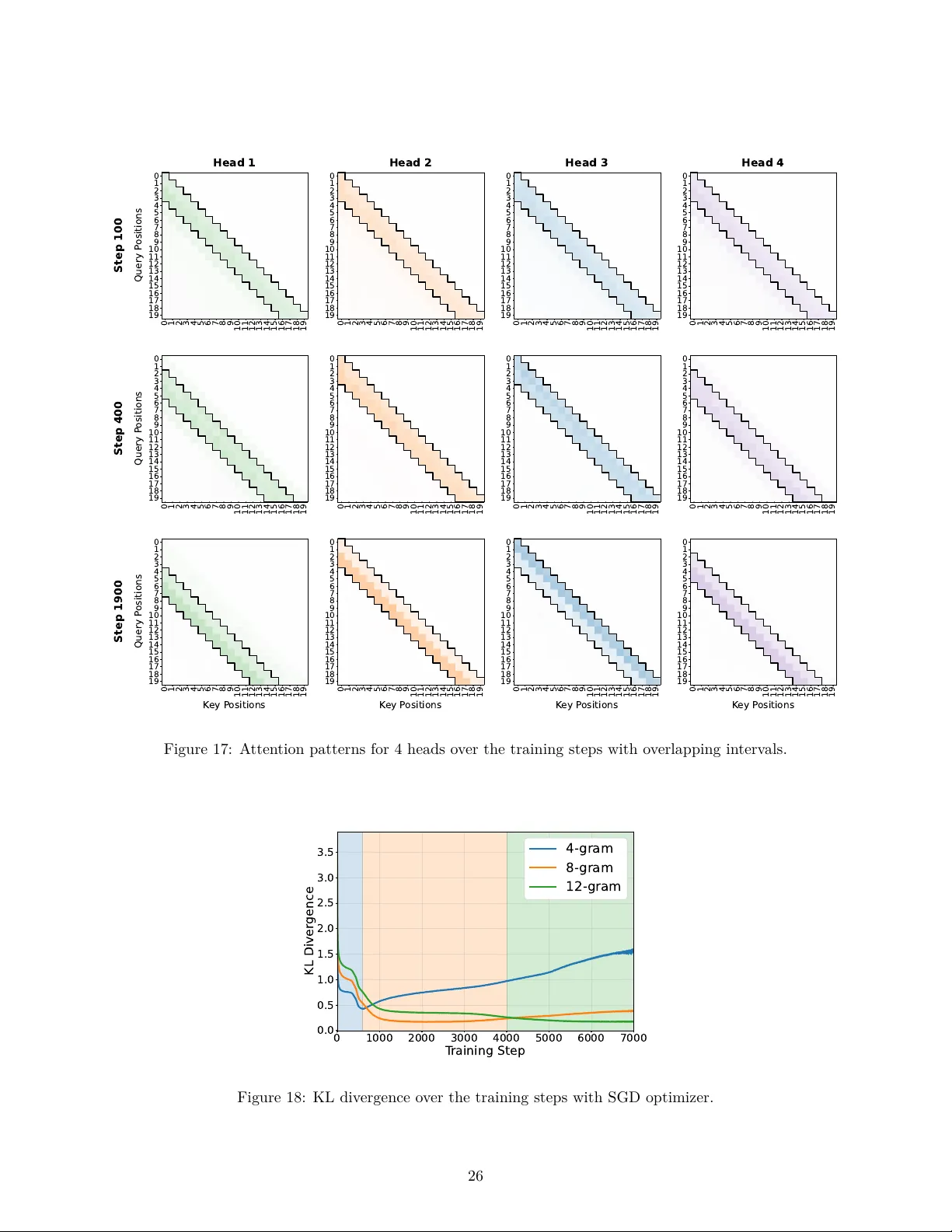
Incremental Lea rning of Spa rse A ttention P atterns in T ransfo rmers Oğuz Kaan Y üksel ∗ o guz.yuksel@epﬂ.ch TML L ab, EPFL Ro drigo Alv arez Lucendo r o drigo.alvar ezluc endo@epﬂ.ch TML L ab, EPFL Nicolas Flammarion nic olas.ﬂammarion@epﬂ.ch TML L ab, EPFL Abstract This pap er introduces a high-order Mark ov c hain task to in vestigate ho w transformers learn to integrate information from multiple past positions with v arying statistical signiﬁcance. W e demonstrate that transformers learn this task incremen tally: eac h stage is deﬁned b y the acquisition of sp eciﬁc information through sparse atten tion patterns. Notably , w e identify a shift in learning dynamics from comp etitiv e, where heads conv erge on the most statistically dominan t pattern, to co op erative, where heads specialize in distinct patterns. W e model these dynamics using simpliﬁed diﬀerential equations that c haracterize the tra jectory and prov e stage-wise con vergence results. Our analysis reveals that transformers ascend a complexit y ladder b y passing through simpler, missp eciﬁed hypothesis classes before reaching the full mo del class. W e further show that early stopping acts as an implicit regularizer, biasing the mo del to ward these simpler classes. These results provide a theoretical foundation for the emergence of staged learning and complex behaviors in transformers, oﬀering insigh ts into generalization for natural language pro cessing and algorithmic reasoning. 1 Intro duction Kno wledge is often comp ositional and hierarc hical in nature. As such, understanding complex concepts often requires an incr emental approach, where simpler concepts are learned ﬁrst and then combined to form more complex ideas. Suc h incremental approaches are crucial for v arious cognitive tasks, including language comprehension, problem-solving, and decision-making in humans and has b een recapitulated in mac hine learning in v arious settings (Saxe et al., 2019). In particular, language, is inheren tly hierarchical, e.g., understanding a sen tence requires understanding the meanings of individual words, phrases, and their structure. Consequen tially , there has been interest in understanding incr emental learning b ehavior of transformers in sequen tial tasks (Abb e et al., 2023b; Edelman et al., 2024), particularly in ho w they build up on previously learned information to understand and generate language (Chen et al., 2024a). The elementary op eration that is needed to comp ose information is c opying , whic h is used to duplicate data and then perform downstream computations. In language, copying is essen tial for tasks such as text generation, where the mo del m ust replicate certain phrases or structures from the input to pro duce coherent and contextually relev ant output (Olsson et al., 2022), and, as a means to aggregate information from m ultiple parts of a text to form a comprehensive understanding. Cop ying is also a fundamental op eration in algorithmic reasoning, where it is often necessary to duplicate intermediate results to p erform further computations. T ransformers implemen t this op eration across diﬀerent p ositions via sparse attention patterns whic h pushes their parameters to diverge . Therefore, the dynamics of ho w these circuits are established ∗ Corresponding author. 1 and its implications on reasoning, generalization and emergence are crucial to grasp the inner workings of transformers. sum of heads Dynamics incr eases Heads L oss incr eases L egend KL Div er gence R epr esentation Head 1 Head 2 Head 3 T ask Figure 1: (T op left) The task is based on a high-order Marko v chain, where the next token dep ends on m ultiple past tokens with diﬀerent imp ortance w eights. The con text is divided in to diﬀerent groups of p ositions, each aggregated and pro cessed b y an asso ciated feature matrix A ⋆ k of v arious imp ortance which is represented by the size of the feature matrix. (T op right) An idealized representation of the task in a m ulti-head single-la y er atten tion. Each head represents an individual sparse attention pattern required to solv e the task. (Bottom left) T ransformers learn the task incrementally , with eac h stage corresp onding to the acquisition of a sparse attention pattern which is indicated by the KL divergence b et ween predictors A ⋆ 1: i that only dep ends a subset of relev ant p ositions as deﬁned in Equation (3) and the transformer. (Bottom right) The learning dynamics transition from comp etitiv e, where all heads fo cus on the statistically most imp ortant pattern (indicated by high combined attention on the main diagonal), to co operative, where diﬀeren t heads sp ecialize in diﬀeren t patterns. In this pap er, we study single-blo ck deco der-based transformers and the formation of sparse attention circuits during training. Simplest such circuit is the “copying” circuit that fo cused on exactly one p osition. It is a sub circuit of well-kno wn induction he ads in transformers (Elhage et al., 2021; Olsson et al., 2022). Sparse atten tion circuits are the building blo cks that allow mo dels to duplicate information from one part of the input to another, enabling the integration of information across multiple p ositions. W e show that they are learned incremen tally , with the mo del ﬁrst acquiring the ability to copy from the most statistically imp ortant pattern, as they provide the most signiﬁcant improv ement in prediction accuracy , and then progressiv ely learning the less imp ortant patterns. In terestingly , w e observ e an initial dynamics where all heads comp ete to learn the most imp ortant pattern, follow ed by a transition to a co op erativ e phase where diﬀeren t heads sp ecialize in diﬀerent patterns. W e explain these dynamics using a set of simpliﬁed diﬀerential equations, after simpliﬁcations to the arc hitecture and the task. This leads to connections to tensor factorization which is a well-studied problem (Arora et al., 2019; Razin et al., 2021; Li et al., 2021; Jin et al., 2023). Our main contributions are as follows: • W e establish the simplest setting for p ositional incremental learning in transformers. In particular, w e isolate the imp ortance of sparse attention patterns as the driving force for incremental learning 2 in transformers, requiring only a single self-attention lay er compared to more in tricate in-context learning settings such as (Edelman et al., 2024). • W e sho w that the learning dynamics transition from comp etitive, where all heads fo cus on the statistically most imp ortant p ositions, to co op erativ e, where diﬀerent heads sp ecialize in diﬀerent p ositions. W e provide a conv ergence result characterizing the initial comp etitive phase as a system of coupled dynamics driven by symmetric initialization. Building on this, we establish conv ergence for the co op erativ e phase b y analyzing the tra jectories initialized in the vicinity of intermediate saddle p oin ts. • W e run studies to understand the impact of the incremental training dynamics on generalization. Dep ending on the size of the training set, mo dels hav e diﬀerent atten tion patterns, e.g., with a smaller training set, the mo del learns to cop y only from the most imp ortant p ositions. This suggests that there is a regularization induced b y the training tra jectories, where transformers are pushed to b e missp eciﬁed dep ending on the size of the training set. With early stopping, this may result in sample complexit y b eneﬁts in low-data regimes. 2 Stage-wise Fo rmation of Spa rse A ttention P atterns In this section, we describ e the data generation pro cess, how transformers can solv e it and the exp erimental evidence to wards incremental learning of sparse attention patterns in transformers. 2.1 Ma rkov Chains with Imp ortance Structure W e consider a sequen tial classiﬁcation task based on a discrete Mark ov c hain of order w with states D = { 1 , . . . , d } . T o facilitate the transition dynamics in a vector space, we represent each state i b y its one-hot enco ding e i ∈ R d . Consequently , eac h element x t in the generated sequence is a one-hot vector. The sequence is initialized by sampling the ﬁrst w tok ens indep enden tly and uniformly: x − w +1 , . . . , x 0 i.i.d. ∼ Unif ( D ) . F or t ∈ [0 , T − 1] , the next state x t +1 is sampled from a categorical distribution whose parameters are determined b y a weigh ted combination of past states: x t +1 ∼ Categorical   softmax   h X k =1 A ⋆ k X i ∈ I ( k ) α i x t − i     , (1) where A ⋆ k ∈ R d × d are ﬁxed feature matrices, I ( k ) are disjoint sets that partition { 0 , . . . , w − 1 } and α i are imp ortance weigh ts which satisfy P i ∈ I ( k ) α i = 1 for all k ∈ [ h ] . This task is simple yet non-trivial and captures some features relev ant to practice: (i) it is sequential, requiring the mo del to in tegrate information from past p ositions, (ii) it has a p ositional structure, as each comp onent of the prediction dep ends on a subset of the past states, and (iii) diﬀerent p ositions can hav e diﬀerent imp ortance, as determined by the feature matrices A ⋆ k and scalars α i . As I ( k ) and A ⋆ k can b e p erm uted without c hanging the data generation pro cess, we assume without loss of generalit y that ∥ A ⋆ 1 ∥ ≥ ∥ A ⋆ 2 ∥ ≥ . . . ≥ ∥ A ⋆ h ∥ and that I (1) con tains the most imp ortant p ositions, i.e., those asso ciated with the largest feature norms. In general, there can b e diﬀerent sp ectrums of imp ortance within eac h feature matrix as well as within each I ( k ) via α i . One particular choice of interest is to hav e I ( k ) to b e con tiguous blo c ks of indices that start from the most recen t p osition, i.e., for some 0 = i 0 < i 1 < i 2 < . . . < i h − 1 < i h = w − 1 , I ( i ) = { i 0 , . . . , i 1 } . (2) This choice is inspired by the natural language where nearby tok ens that complete the text into a word or a short phrase should hav e more statistical correlation ov er the distant tokens. Notably , when each of 3 0 1 2 3 4 5 6 7 8 9 10 11 12 13 14 15 16 17 18 19 K ey P ositions 0 1 2 3 4 5 6 7 8 9 10 11 12 13 14 15 16 17 18 19 Query P ositions S t e p 0 0 1 2 3 4 5 6 7 8 9 10 11 12 13 14 15 16 17 18 19 K ey P ositions 0 1 2 3 4 5 6 7 8 9 10 11 12 13 14 15 16 17 18 19 S t e p 6 0 0 1 2 3 4 5 6 7 8 9 10 11 12 13 14 15 16 17 18 19 K ey P ositions 0 1 2 3 4 5 6 7 8 9 10 11 12 13 14 15 16 17 18 19 S t e p 3 0 0 0 1 2 3 4 5 6 7 8 9 10 11 12 13 14 15 16 17 18 19 K ey P ositions 0 1 2 3 4 5 6 7 8 9 10 11 12 13 14 15 16 17 18 19 S t e p 1 0 0 0 Figure 2: The sum of learned attention patterns for h = 3 , w = 12 at diﬀerent stages of training where blue, y ello w and green colors corresp ond to diﬀerent heads. A t t = 0 , the attention is uniform as the mo del is randomly initialized. A t t = 60 , all heads learn from the p ositions in I (1) , indicated by the o verlappin g blue, y ello w and green colors, with one head fo cusing on the p ositions in I (2) with a small attention. At t = 300 , a head learns from the p ositions in I (2) whereas tw o heads still fo cus on I (1) . At t = 1000 , the mo del ﬁnally learns to integrate all p ositions where each head specializes in a diﬀeren t pattern. The main diagonal do es not ha v e the same intensit y as the other p ositions as it is learned via the skip connection directly from the input. the I ( k ) are singletons, the resulting op eration is copying from a particular p osition and then pro cessing it with a linear feature map. The “copying” op eration is of particular interest as it app ears in v arious settings including in-con text learning (Brown et al., 2020). 2.2 T ransfo rmers Learn Incrementally W e train single-blo c k deco der-based transformers with h heads on sequences sampled as in Equation (1) b y minimizing the cross entrop y loss ov er the full sequence except the initial tokens x − w +1 , . . . , x 0 that are not sampled from the pro cess. W e keep the architecture as close to the standard practice as p ossible. The arc hitecture and optimization details are provided in App endix A. W e sample feature matrices A ⋆ k uniformly o v er orthogonal matrices and then scale with p ositive scalars m k . These constants are chosen geometrically , i.e., m k = m h − k b 0 where m > 1 is the multiplicativ e constant and b 0 > 0 is the base scale. This results in an imp ortance hierarch y in the feature matrices whereas features within the same matrix has the same imp ortance. In particular, A ⋆ 1 has the largest norm and thus contains the most inﬂuential features in the pro cess whereas A ⋆ k has the smallest norm and thus the least imp ortant features. F or simplicity , we c ho ose α i = 1 / | I ( I − 1 ( i )) | where I − 1 is the inv erse of I . Lastly , we choose I ( k ) as in Equation (2) with the same length interv als of size w /h . These choices formalize the notion of relative imp ortance b etw een lo cal p ositions ov er the distan t p ositions. As I (1) is paired with A ⋆ 1 that has a large norm, the nearby p ositions inﬂuence the next token more that the distan t tokens in I ( h ) that are paired with A ⋆ h whic h has a small norm. The details of all exp erimen tal parameters are provided in App endix A and additional exp erimen ts can b e found in App endix B. W e observ e that the transformers learn the task incremen tally , with each stage corresponding to the acquisition of a sparse attention pattern as in Figure 2. All heads start at uniform due to the initialization. Then, they ﬁrst mainly focus on the p ositions in I (1) as they are the most statistically imp ortant p ositions. A t this stage, the heads comp ete to learn from these p ositions, resulting in o verlapping attention patterns with some deviations due to the initialization. Later, heads gradually sp ecialize in diﬀerent patterns, with one head learning from the p ositions in I (2) while the other ﬁnally fo cusing on I (3) . In order to understand the dynamics in the function space, we train mo dels with diﬀerent maximum context lengths c = 4 , 8 , 12 . When c = 4 , the mo del can only access the p ositions in I (1) and th us learns only from these p ositions. When c = 8 , the mo del can access the p ositions in I (1) and I (2) and when c = 12 , the mo del can access all the relev ant p ositions and can implement the task p erfectly . In Figure 3 (right), we plot the Kullbac k-Leibler (KL) divergence b et ween the predictions of these transformers and the transformer without 4 0 100 200 300 400 500 600 700 800 900 1000 T raining Step 0.5 1.0 1.5 2.0 2.5 3.0 3.5 KL Diver gence A * 1 A * 1 : 2 A * 1 : 3 0 100 200 300 400 500 600 700 800 900 1000 T raining Step 0.5 1.0 1.5 2.0 2.5 3.0 KL Diver gence 4-gram 8-gram 12-gram Figure 3: (Left) KL divergence b etw een the ground truths that only dep end on the p ositions in I (1) , I (1) ∪ I (2) and I (1) ∪ I (2) ∪ I (3) , and the predictions of the transformer with unrestricted context length. (Righ t) KL divergence b et ween the predictions of the transformers with restricted context lengths c = 4 , 8 , 12 and the transformer without any context length restriction. The transformers learn the task incrementally , with eac h stage corresp onding to the acquisition of information from a subset of p ositions. an y context length restriction. W e observe that the transformers ﬁrst approach the mo del with c = 4 and then c = 8 b efore ﬁnally reac hing the full mo del with c = 12 . This indicates that the transformers not only learn the attention patterns but also simultaneously learn the feature matrices asso ciated with these patterns. Similarly , w e study the KL divergence pattern when comparing the predictions of the transformers to the ground truths that only dep end on the p ositions in I (1) , I (1) ∪ I (2) and I (1) ∪ I (2) ∪ I (3) : f A ⋆ 1: i = softmax   i X k =1 A ⋆ k X j ∈ I ( k ) α j x t − j   . (3) This is plotted in Figure 3 (left) where we see an iden tical pattern. These are similar to what Edelman et al. (2024) observ ed for in-context Marko v chain where stages are characterized by sub- n -grams. 2.3 Rep resentation with a Simpli ﬁed Multi-Head Attention Here, we construct a simple representation on a single-lay er m ulti-head attention that solves the task. Let X ∈ R d × ( T + w ) b e the input data matrix with columns x − w +1 , . . . , x 0 , x 1 , . . . , x T . W e assume that the p ositional information is enco ded using one-hot vectors in R T and concatenated to the data as follows: ˜ X =  X I T + w  ∈ R ( d + T + w ) × ( T + w ) . W e denote the columns of ˜ X as ˜ x i ∈ R d + T + w , represen ting the p osition-augmented embedding of the i -th tok en. Then, the transformer tak es ˜ X as input and pro duces the output Y ∈ R d × T with columns y 0 , . . . , y T − 1 as follo ws: y t = softmax h X k =1 V k ˜ X a ( k ) t ! , with a ( k ) t = softmax  M T − t  ˜ X ⊤ K ⊤ k Q k ˜ x t  , where Q k , K k , V k ∈ R ( d + T + w ) × ( d + T + w ) are the query , k ey and v alue matrices of the head k , resp ectively and M p sets the last p entries to −∞ to apply causal masking. 5 0 200 400 600 800 1000 T raining Step 0.0 0.5 1.0 1.5 2.0 2.5 3.0 Ex cess L oss 1 1 0 3 1 0 6 1 0 9 0 0 200 400 600 800 1000 T raining Step 0.0 0.5 1.0 1.5 2.0 2.5 3.0 Ex cess L oss 1.0 1.3 1.5 Figure 4: (Left) Excess loss of the minimal architecture with diﬀerent initialization scales. (Righ t) Excess loss of the minimal architecture with diﬀerent multiplicativ e constants m that determine the imp ortance hierarc h y . F or head k , we set the v alue matrix V k = A ⋆ k and a ( k ) t to b e a p ositional-only attention corresp onding to I ( k ) with the following sparse pattern 1 | I ( k ) |    0 , . . . , 0 | {z } t entries , 1 ( w − 1) ∈ I ( k ) , 1 ( w − 2) ∈ I ( k ) , . . . , 1 0 ∈ I ( k ) | {z } w entries , 0 , . . . , 0 | {z } ( T − t ) entries    . Here, the ﬁrst t en tries corresp ond to the irrelev ant tokens in the context and the last ( T − t ) entries are zero ed out due to the causal masking. Among the relev ant tokens in the intermediate w p ositions, the atten tion fo cuses on the indices in I ( k ) as they can b e pro cessed altogether with the same feature matrix V k = A ⋆ k . As the target patterns are sparse, the parameters of the attention need to diverge to inﬁnity to exactly learn this op eration. In practice, we exp ect ﬁnite v alues that approximate these sparse attention patterns. These atten tion patterns can b e learned based on the p ositional information: K ⊤ k Q k = λ X i ∈ I ( k ) T + w X p = w e d + p − i e ⊤ d + p , where λ > 0 is a scaling constan t and e i is the i -th standard basis vector in R d + T . As λ → ∞ , the attention scores con verge to the desired sparse pattern. Note that this construction is not unique as there are man y Q k and K k that can realize the same attention pattern. In particular, there is a symmetry where ( Q k , K k ) can b e replaced with  M − 1 Q k , M ⊤ K k  for an y in v ertible matrix M without changing the attention scores. Moreov er, as there are h heads to learn, the construction has a p ermutation symmetry . The p ermutation symmetry is key in understanding the learning dynamics, as we discuss in Section 3.2. 2.4 Ablation Studies In order to isolate the essential comp onents that drive the incremental learning b ehavior, we simplify the arc hitecture b y removing some comp onents. First, we remov e an y comp onen ts such as lay er normalization and residual connections that are not present in the idealized construction in Section 2.3. Then, we reduce the pro duct K ⊤ k Q k to a single matrix A k as there is a symmetry b etw een K k and Q k . All of these c hanges individually or com bined do not alter the incremental learning b ehavior. W e plot the learning b ehavior of this simpliﬁed mo del in Figure 1. W e also p erform ablation studies with this minimal architecture. W e ﬁrst v ary the initialization scale of the atten tion matrices A k and set v alue matrices to b e zero. While initializing A k , w e use uniform distribution 6 o v er [ − u, u ] where u is the initialization scale. Figure 4 (left) sho ws that the sp eed of incremental learning is aﬀected by the initialization scale, with smaller scales resulting in slow er learning. A t the extreme u = 0 , we observ e that the mo del only learns a single pattern and do es not progress further. This is b ecause of the symmetry b et ween the heads, which requires a small p erturbation to break. W e also v ary the m ultiplicativ e constan t m that determines the structure in the data generation pro cess. Figure 4 (right) shows that the n umber of steps diminish to tw o for m = 1 , where there is no imp ortance ordering. Qualitativ ely , this mo del ﬁrst learns a single pattern and then the other tw o are learned sim ultane- ously . F or m = 1 . 3 and m = 1 . 5 , w e still observe three distinct stages, but the stages are intert wined for m = 1 . 3 and bumps are less pronounced. 2.5 Dataset Size and Generalization Lastly , we study the eﬀect of the dataset size on the incremental learning b ehavior. As we decrease the dataset size and cross some critical thresholds, we observe that the num b er of stages that o ccur in training decreases, as seen in Figure 5 (left). Figure 5 (righ t) plots the KL divergence b et ween the predictions of the mo del with diﬀerent context lengths and the trained transformer. The trend is similar to the one observed in Figure 3 but with diﬀerent num b er of bumps for each dataset size. This p oin ts tow ards a b eneﬁcial regularization from the training tra jectory whic h leads to missp eciﬁed mo dels, i.e., mo dels that are not able to learn the task p erfectly as they hav e a shorter context length. Yüksel et al. (2025) argue that such missp eciﬁcation can b e b eneﬁcial in lo w-data regimes, making learning statistically feasible. Notably , transformers with early stopping seem to select the missp eciﬁcation length automatically , hin ting at p oten tial sample complexity gains in these settings. 0 250 500 750 1000 Step 0 1 2 3 Best Ex cess L oss 0 250 500 750 1000 Step 1 2 3 4 5 KL Diver gence 6 0 0 s a m p l e s 0 250 500 750 1000 Step 1 2 3 4 2 0 0 0 s a m p l e s 0 250 500 750 1000 Step 0 1 2 3 9 0 0 0 s a m p l e s 600 2000 9000 online 4-gram 8-gram 12-gram Figure 5: The impact of the dataset size on the incremental learning b ehavior. (Left) The b est v alidation loss as a function of the dataset size. (Righ t) The KL div ergence b et w een the predictions of the mo del with diﬀeren t context lengths and the trained transformer. Dashed lines indicate the ﬁrst step that obtains the b est excess loss. 3 T raining Dynamics on Regression V ariant In this section, we study the regression v ariant of the classiﬁcation task in Section 2.1. W e study the resulting training dynamics by analyzing the gradient ﬂow dynamics of the loss. 3.1 The Regression Mo del Consider the following regression task asso ciated to any distribution P X and P ξ : ( x 1 , . . . , x T ) ∼ P X , ξ ∼ P ξ , and y ⋆ ( X ) = h X k =1 A ⋆ k X s ⋆ k + ξ , 7 where s ⋆ k ∈ R T is the vector with entries α i for i ∈ I ( k ) and zero otherwise. F or this section, we set | I ( k ) | = 1 for all k for simplicity . Let m ⋆ k = ∥ A ⋆ k ∥ F , V ⋆ k = A ⋆ k m ⋆ k for all k ∈ [ h ] with m ⋆ 1 > . . . > m ⋆ h without loss of generalit y . W e make some assumptions regarding the distributions P X , P ξ and the feature matrices. Assumption 1. The noise is zer o-me an, i.e., E [ ξ ] = 0 and the data is normalize d, i.e., ∀ i, j ∈ [ T ] , E  x i x ⊤ j  = 1 i = j I d . Assumption 2. The fe atur e matric es ar e ortho gonal, i.e., ∀ i, j ∈ [ h ] , ⟨ V ⋆ i , V ⋆ j ⟩ = T r  ( V ⋆ i ) ⊤ V ⋆ j  = 1 i = j . W e use the minimal architecture obtained in Section 2.4 with the following mo diﬁcations. The attention scores are computed only via the inner pro duct of p osition vectors instead of the concatenated p osition and data vectors. As the problem is a regression task on the ﬁnal token, we only need the last row of the matrix Q k whic h we denote by q k ∈ R T . Then, the resulting mo del is as follows: y θ ( X ) = h X k =1 V k X s k , with s k = softmax( q k ) , where θ = ( V 1 , . . . , V h , q 1 , . . . , q h ) are the learnable parameters. W e set the loss to the mean square loss: L ( θ ) = 1 2 E x 1 ,...,x T ,ξ  ∥ y θ ( X ) − y ⋆ ( X, ξ ) ∥ 2  . (4) W e study the gradient ﬂow dynamics of the p opulation loss in Equation (4), i.e., we consider the con tinuous- time limit of gradient descent with inﬁnitesimal step size. T ensor Notation. W e construct tensors that are sum of outer pro ducts of matrices and v ectors, i.e., M = P h k =1 B k ⊗ v k where B k ∈ R d × d and v k ∈ R T . The pro duct X ⊤ M denotes X ⊤ M = P h k =1 ⟨ B k , X ⟩ v k whereas the pro duct M v denotes M v = P h k =1 B k ⟨ v k , v ⟩ . The inner pro duct b etw een tw o tensors M = P h k =1 B k ⊗ v k and N = P h k =1 B ′ k ⊗ v ′ k is denoted by ⟨ M , N ⟩ = P h k =1 ⟨ B k , B ′ k ⟩⟨ v k , v ′ k ⟩ . The F rob enius norm of a tensor M is giv en b y ∥ M ∥ F = p ⟨ M , M ⟩ . Prop osition 1 rein terprets this dynamics as a gradient ﬂow of a tensor factorization problem. Prop osition 1. The gr adient ﬂow dynamics of the loss in Equation (4) is e quivalent to that on L ( θ ) = 1 2 ∥ G − P ∥ 2 F wher e P = h X k =1 V k ⊗ s k , and G = h X k =1 m ⋆ k ( V ⋆ k ⊗ s ⋆ k ) . A ttention Reparameterization. Note that due to the softmax op eration, P i q i is alw ays constant and th us we can restrict q k to hav e a zero mean without loss of generality . This implies that, there is a one-to-one corresp ondence b et ween q k and s k in the subspace of zero-mean vectors. Therefore, it is p ossible to analyze the dynamics in terms of s k instead of q k with the notation Π( s ) =  diag( s ) − ss ⊤  : ˙ V k = ( G − P ) s k , ˙ s k = Π( s k ) 2  V ⊤ k ( G − P )  . Numerical Sim ulations. W e simulate these diﬀerential equations with initialization V i = 0 and s i ≈ 1 T 1 T . The results recapitulate the incremental learning b ehavior observ ed in Figure 2. W e present the results in Section B.4. 8 3.2 Coupled Dynamics Describ e the Comp etitive Phase W e sho w that the comp etitive phase of the learning dynamics can b e described by the symmetric initialization s 1 (0) = s k (0) , V 1 (0) = V k (0) for all k . Once the heads are coupled, they co evolv e, i.e., s k (0) = s (0) , V k (0) = V (0) for all k . This leads to the following coupled dynamics: ˙ V =  G s − h ∥ s ∥ 2 V  , ˙ s = Π( s ) 2  V ⊤ G − h ∥ V ∥ 2 F s  . Theorem 1. A ssume that the initialization veriﬁes the fol lowing for al l k ∈ [ h ] : ⟨ V (0) , V ⋆ 1 ⟩ ≥ ⟨ V (0) , V ⋆ k ⟩ , ⟨ s (0) , s ⋆ 1 ⟩ ≥ ⟨ s (0) , s ⋆ k ⟩ . (5) Then, the dynamics of V and s c onver ge to the fol lowing ﬁxe d p oint: V ( ∞ ) = m ⋆ 1 h V ⋆ 1 , s ( ∞ ) = s ⋆ 1 . (6) Theorem 1 is based on an ordering argument. As long as the initialization veriﬁes the ordering condition in Equation (5), the dynamics of V and s are such that ˙ V and ˙ s reinforces the same order. Standalone, Theorem 1 do es not explain what happens when the heads do not start with the same initialization. Theorem 2 establishes that when many heads are initialized with a small deviation from the symmetric initialization, the deviation from the symmetric initialization is b ounded for a ﬁnite time that we can precisely control. Therefore, the initialization chooses the coupling time of diﬀerent heads after which they migh t start to div erge. Theorem 2. A ssume that the fol lowing holds for ϵ ≪ 1 : ∀ k ∈ [ h ] : ∥ V (0) − V k (0) ∥ F ≤ ϵ and ∥ s (0) − s k (0) ∥ 2 ≤ ϵ . Then, ther e exists a c onstant c 1 such that ∀ t ∈ h 0 , 1 − c 1 log ϵ i : ∥ V k ( t ) − V ( t ) ∥ F ≤ ϵe c 1 t and ∥ s k ( t ) − s ( t ) ∥ 2 ≤ ϵe c 1 t . Lastly , we remark that the initialization in Theorem 1 can b e further relaxed to a wider basin of attraction around the symmetric initialization of interest. This follows from a similar argument as in Zucc het et al. (2025) who has studied the escap e time from this initialization when h = 1 . Remark 1. The initialization of inter est is s k (0) ≈ 1 T 1 T for al l k ∈ [ h ] as se en in Figur e 2. By exp anding the dynamics ar ound this initialization with V k ≈ 0 for al l k ∈ [ h ] , we get: ˙ V k (0) ≈ 1 T G 1 T , ˙ s k (0) ≈ 0 . Similarly, se c ond-or der lo c al appr oximation shows that s k has the lar gest incr e ase towar ds the dir e ction s ⋆ 1 . Ther efor e, we c an quantify a wider b asin of attr action for The orem 1 as al l V k and s k move towar ds the initialization sp ac e deﬁne d by Equation (5) . 3.3 Co op eration After Comp etition In order to study the co op erative phase after the initial comp etitive phase, we consider the dynamics of the loss at v arious initializations around the ﬁxed p oint in Equation (6). Consider the following initialization sc heme: V 1 (0) = . . . = V h − 1 (0) ≈ m ⋆ 1 h V ⋆ 1 , V h (0) ≈ m ⋆ 1 h V ⋆ 1 , s 1 (0) = . . . = s h − 1 (0) = s ⋆ 1 , s h ≈ s ⋆ 1 . (7) 9 The dynamics of s 1 , . . . , s h − 1 remain constan t due to the pro jection. In addition, V 1 , . . . , V h − 1 are coupled due to the gradien t ﬂo w. Therefore, the whole system collapses to the three equations, one for V that describ es the ensem ble and tw o V ′ , s ′ that describ es the oﬀsho oting head: ˙ s ′ = Π( s ′ ) 2  V ′⊤ G − ( h − 1) ⟨ V ′ , V ⟩ s ⋆ 1 − ∥ V ′ ∥ 2 s ′  , ˙ V = m ⋆ 1 ∥ s ⋆ 1 ∥ 2 V ⋆ 1 − ( h − 1) ∥ s ⋆ 1 ∥ 2 V − ⟨ s ⋆ 1 , s ′ ⟩ V ′ , ˙ V ′ = G s ′ − ( h − 1) ⟨ s ⋆ 1 , s ′ ⟩ V − ∥ s ′ ∥ 2 V ′ , (8) W e hav e a similar control to Theorem 2 for the dynamics of V , V ′ and s ′ . Theorem 3 establishes that the deviation from the co op erative system is b ounded for a ﬁnite time that w e can precisely con trol. This is due to a Lyapuno v control argument where the norms of V and V ′ are b ounded. Theorem 3. A ssume that the fol lowing holds for ϵ ≪ 1 : ∀ k ∈ [ h − 1] : ∥ V (0) − V k (0) ∥ F ≤ ϵ, ∥ e 1 − s k (0) ∥ 2 ≤ ϵ , and ∥ V ′ (0) − V h (0) ∥ F ≤ ϵ , ∥ s ′ (0) − s h (0) ∥ 2 ≤ ϵ . L et ∆( t ) b e the deviation fr om the c o op er ative system in Equation (8) : ∆( t ) = max n max k {∥ V k ( t ) − V ( t ) ∥ F , ∥ s k ( t ) − s ( t ) ∥ 2 } , ∥ V h ( t ) − V ( t ) ∥ F , ∥ s h ( t ) − s ( t ) ∥ 2 o . A ssuming that ∥ s ′ ( t ) − s ⋆ 1 ∥ ≥ δ for al l t ∈ R , ther e exists a universal c onstant c 1 such that: ∆( t ) ≤ ϵe c 1 t , ∀ t ∈  0 , 1 − c 1 log ϵ  . The dynamics in Equation (8) is interesting as while V ′ gro ws in an orthogonal direction V ⊥ to V ⋆ 1 , s ′ is still sparse around s ⋆ 1 . This is due to the fact that Π( s ′ ) ≈ 0 at initialization as s ′ (0) ≈ s ⋆ 1 whic h leads to a scale separation b etw een ˙ s ′ and ˙ V ′ . Consequen tially , when V ′ gro ws along some V ⊥ , the prediction is pushed to include the unnecessary term, V ⊥ x t . Ho wev er, this is instantly cancelled out by the progression of the ensem ble, where V learns to oﬀset this by learning − V ⊥ . This collab orative b ehavior is b est seen in our plots in Figure 10. T o simplify Equation (8), we show that the initialization in Equation (7) ensures that V is close to its optimal v alue, V ⋆ , which is deﬁned in Lemma 1. In fact, we can derive a precise statemen t ab out how far V is from V ⋆ based on how muc h weigh t s ′ puts on the directions that are orthogonal to s ⋆ 1 : Lemma 1. L et ∆( t ) = V ( t ) − V ⋆ ( t ) wher e V ⋆ ( t ) = 1 h − 1 ( m ⋆ 1 V ⋆ 1 − ⟨ s ⋆ 1 , s ′ ( t ) ⟩ V ′ ( t )) . A ssuming that ∥ s ′ ( t ) − s ⋆ 1 ∥ ≥ δ for al l t ∈ R , ther e exist c onstants c 1 ( δ ) , c 2 such that ∥ ∆( t ) ∥ F ≤ e − c 2 t ∥ ∆(0) ∥ F + c 1 ( δ ) c 2 . Inspired b y Lemma 1 and numerical simulations, we approximate the full dynamics by a tw o-scale analysis where V is optimized faster, leading to the following dynamics: ˙ V ′ = G (1) s ′ (1) − ∥ s ′ (1) ∥ 2 V ′ , ˙ s ′ = Π( s ′ ) 2  V ′⊤ (1) G (1) − ∥ V ′ ∥ 2 F s ′ (1)  , (9) where w e introduce the following notation: G ( i ) = G − i X j =1 m ⋆ j  V ⋆ j ⊗ s ⋆ j  , V ( i ) = V − i X j =1 ⟨ V ⋆ j , V ⟩ V ⋆ j , s ( i ) = s − i X j =1 ⟨ s ⋆ j , s ⟩ s ⋆ j . W e show that dynamics in Equation (9) con v ergences to the second p ositional feature: 10 Theorem 4. A ssume that the initialization veriﬁes the fol lowing for al l k ∈ [2 , h ] : ⟨ V ′ (0) , V ⋆ 2 ⟩ ≥ ⟨ V ′ (0) , V ⋆ k ⟩ ⟨ s ′ (0) , s ⋆ 2 ⟩ ≥ ⟨ s ′ (0) , s ⋆ k ⟩ . F urther, supp ose that V ′ (0) , s ′ (0) ar e such that ⟨ V ′ (1) (0) , G (1) s ′ (1) (0) ⟩ > 1 2 ∥ V ′ (0) ∥ 2 F ∥ s ′ (1) (0) ∥ 2 . (10) Then, the dynamics of V ′ and s ′ c onver ge to the fol lowing ﬁxe d p oint: V ′ ( ∞ ) = V ⋆ 2 , s ′ ( ∞ ) = s ⋆ 2 . Theorem 4 is similar in nature to Theorem 1. Once there is an alignment to the second p ositional feature, the dynamics is such that the alignment is not broken. Notably , we require the initialization to satisfy Equation (10). This is to ensure that the dynamics start with an initial decrease on the loss b eyond the ﬁrst saddle p oint characterized in Theorem 4. Theorem 4 prov es that a p otential that characterizes the loss is monotonically minimized and this saddle is av oided. In Remark 2, we discuss how a small p erturbation to w ards the second p ositional feature is suﬃcient to satisfy Equation (10). Finally , in Section C.4, we extend our analysis to the sp ecialization of an arbitrary head n after the system has acquired the ﬁrst n − 1 features. Analogously to our previous deriv ation, we assume a single “free” head while the remainder of the ensem ble is ﬁxed at its optimal conﬁguration. In contrast to the tw o-head case, we supp ose that heads 2 through n − 1 hav e already sp ecialized to p ositions 2 through n − 1 , while all remaining heads, excluding the free one, retain the ﬁrst feature and op erate co operatively with it. 4 Related Wo rk Our w ork is at the intersection of incremental learning, n - gram mo dels and dynamics of attention. Incremen tal learning. Plateau-lik e learning curves are a common feature in neural net work training. Early analyses, such as F ukumizu & Amari (2000), attributed these b ehaviors to critical p oints in sup ervised learning. Subsequent studies hav e examined similar dynamics in a v ariety of simpliﬁed settings, including linear netw orks (Gissin et al., 2020; Saxe et al., 2019; Gidel et al., 2019; Arora et al., 2019; Jacot et al., 2021; Li et al., 2021; Razin et al., 2021; Jiang et al., 2022; Berthier, 2022; Pesme & Flammarion, 2023; Jin et al., 2023; V arre et al., 2023; 2024), ReLU mo dels (Boursier et al., 2022; Abb e et al., 2023a), simpliﬁed transformer arc hitectures (Boix-Adsera et al., 2023), and recent work argues for their universalit y (Ziyin et al., 2025; Kunin et al., 2025; Zhang et al., 2025a). In transformer training, plateaus follow ed by sudden capability gains (Chen et al., 2024a; Kim et al., 2024) are often observed in regression tasks (Garg et al., 2022; V on Oswald et al., 2023; Ahn et al., 2024), formal language recognition (Bhattamishra et al., 2023; Akyürek et al., 2024; D’Angelo et al., 2025; Cagnetta et al., 2025). Finally , Cagnetta & W yart (2024); Cagnetta et al. (2025) study the eﬀect of dataset size in learning random probabilistic context-free grammars, showing that the order of the learned hierarch y dep ends on data av ailability , a dynamic similar to the data-dep enden t stage progression in our observ ations. n -gram mo dels. n -gram language mo dels (Jurafsky & Martin, 2009) serve as a toy setting to understand large language mo dels. This p ersp ective has motiv ated a range of studies: the optimization landscap e has b een characterized in Makkuv a et al. (2024), expressivit y ov er n -gram distributions has b een examined in Sv ete & Cotterell (2024) and sample complexity has b een resolved in Yüksel & Flammarion (2025). Learning of v ariable-order n -grams ha v e b een studied b y (Zhou et al., 2024) whereas (Deora et al., 2025) consider n -grams with diﬀerent order. Connections b etw een ICL and the emergence of induction heads (Elhage et al., 2021; Olsson et al., 2022), together with their acquisition via gradient descent (Nichani et al., 2024), are drawn by Bietti et al. (2023). T raining dynamics on n -gram prediction tasks ha v e also been sho wn to progress in stages: intermediate solutions appro ximate sub- n -grams (Edelman et al., 2024; Chen et al., 2024b), whic h later are formalized as near-stationary p oin ts by V arre et al. (2025). Despite leading to ric h 11 phenomenology , n -grams are typically studied without any inherent hierarhical abstractions that are presen t in natural language (W u et al., 2022; 2025). W e also use a simpliﬁed syn thetic data to isolate the phenomenon of study . Dynamics of attention. The dynamics of attention ha ve recen tly b een explored through v arious simpliﬁed mo dels. Sp eciﬁcally , (Snell et al., 2021) examine a “bag-of-words” proxy , while (Jelassi et al., 2022) in vestigate a simpliﬁed Vision T ransformer (ViT) restricted to position-only atten tion. Under a masked language mo deling ob jective, (Li et al., 2023) characterize a tw o-stage training regime. F urther theoretical analyses include the sto chastic gradient dynamics of p osition-free attention (Tian et al., 2023), the evolution of diagonal atten tion w eights (Abb e et al., 2023b), and the b eha vior of linear attention within the framework of in-context linear regression (Zhang et al., 2025b). P articularly relev ant to our data mo del, (Marion et al., 2025) study training tra jectories in single-lo cation regression, a setting related to sequence multi-index mo dels (Cui et al., 2024; T roiani et al., 2025). Closest to our work, (Zucchet et al., 2025) consider the single-head case h = 1 and analyze the escap e time from the initialization V = 0 , s = 1 T 1 T . While their analysis relies on a lo cal T a ylor approximation around this initialization, we characterize the full stage-wise saddle-to-saddle dynamics that emerge following the initial escap e. 5 Conclusion In this work, we introduce a simple yet theoretically rich task requiring transformers to implement multiple sparse attention patterns. W e demonstrate that this task captures the core mec hanics of p osition-dep endent, incremen tal learning. Our analysis rev eals a distinct phase transition: the dynamics b egin in a comp etitive regime, where heads conv erge on the most statistically salient pattern, b efore transitioning into a co op erative regime c haracterized by head sp ecialization. W e formalize these observ ations through rigorous con vergen ce results within a simpliﬁed regression framework that c haracterizes the underlying training dynamics. Our ﬁndings highlight the intricate interpla y b etw een attention sparsit y and transformer learning dynamics—a connection that is fundamental to understanding how these mo dels scale to complex reasoning and natural language pro cessing tasks. A cknowledgments This project w as supp orted b y the Swiss National Science F oundation (grant num b er 212111) and an unrestricted gift from Go ogle. References Emman uel Abb e, Enric Boix Adsera, and Theo dor Misiakiewicz. Sgd learning on neural netw orks: leap complexit y and saddle-to-saddle dynamics. In The Thirty Sixth A nnual Confer enc e on L e arning The ory , pp. 2552–2623. PMLR, 2023a. Emman uel Abb e, Samy Bengio, Enric Boix-Adserà, Etai Littwin, and Joshua M. Susskind. T ransformers learn through gradual rank increase. In Alice Oh, T ristan Naumann, Amir Globerson, Kate Saenk o, Moritz Hardt, and Sergey Levine (eds.), A dvanc es in Neur al Information Pr o c essing Systems 36: A n- nual Confer enc e on Neur al Information Pr o c essing Systems 2023, NeurIPS 2023, New Orle ans, LA, USA, De c emb er 10 - 16, 2023 , 2023b. URL http://papers.nips.cc/paper_files/paper/2023/hash/ 4d69c1c057a8bd570ba4a7b71aae8331- Abstract- Conference.html . K w ang jun Ahn, Xiang Cheng, Hadi Daneshmand, and Suvrit Sra. T ransformers learn to implement preconditioned gradien t descent for in-context learning. A dvanc es in Neur al Information Pr o c essing Systems , 36, 2024. Ekin Akyürek, Bailin W ang, Y o on Kim, and Jacob Andreas. In-con text language learning: Arhitectures and algorithms. arXiv pr eprint arXiv:2401.12973 , 2024. 12 Sanjeev Arora, Nadav Cohen, W ei Hu, and Y uping Luo. Implicit regularization in deep matrix factorization. A dvanc es in Neur al Information Pr o c essing Systems , 32, 2019. Raphaël Berthier. Incremen tal learning in diagonal linear netw orks. arXiv pr eprint arXiv:2208.14673 , 2022. Sat wik Bhattamishra, Arkil Patel, Phil Blunsom, and V arun Kanade. Understanding in-context learning in transformers and llms by learning to learn discrete functions. arXiv pr eprint arXiv:2310.03016 , 2023. Alb erto Bietti, Vivien Cabannes, Diane Bouc hacourt, Hervé Jégou, and Léon Bottou. Birth of a transformer: A memory viewpoint. In Alice Oh, T ristan Naumann, Amir Glob erson, Kate Saenk o, Moritz Hardt, and Sergey Levine (eds.), A dvanc es in Neur al Information Pr o c essing Systems 36: A n- nual Confer enc e on Neur al Information Pr o c essing Systems 2023, NeurIPS 2023, New Orle ans, LA, USA, De c emb er 10 - 16, 2023 , 2023. URL http://papers.nips.cc/paper_files/paper/2023/hash/ 0561738a239a995c8cd2ef0e50cfa4fd- Abstract- Conference.html . Enric Boix-A dsera, Etai Littwin, Emmanuel Abb e, Sam y Bengio, and Joshua Susskind. T ransformers learn through gradual rank increase. arXiv pr eprint arXiv:2306.07042 , 2023. Etienne Boursier, Loucas Pillaud-Vivien, and Nicolas Flammarion. Gradien t ﬂow dynamics of shallo w reLU net works for square loss and orthogonal inputs. In Alice H. Oh, Alekh Agarwal, Danielle Belgrav e, and Kyungh yun Cho (eds.), A dvanc es in Neur al Information Pr o c essing Systems , 2022. URL https: //openreview.net/forum?id=L74c- iUxQ1I . T om B. Bro wn, Benjamin Mann, Nick R yder, Melanie Subbiah, Jared Kaplan, Prafulla Dhariwal, Arvind Nee- lakan tan, Pranav Shy am, Girish Sastry , Amanda Askell, Sandhini Agarw al, Ariel Herb ert-V oss, Gretchen Krueger, T om Henighan, Rewon Child, A dity a Ramesh, Daniel M. Ziegler, Jeﬀrey W u, Clemens Winter, Christopher Hesse, Mark Chen, Eric Sigler, Mateusz Litwin, Scott Gray , Benjamin Chess, Jack Clark, Christopher Berner, Sam McCandlish, Alec Radford, Ilya Sutskev er, and Dario Amo dei. Language mo dels are few-shot learners. In Hugo Laro chelle, Marc’Aurelio Ranzato, Raia Hadsell, Maria-Florina Balcan, and Hsuan-Tien Lin (eds.), A dvanc es in Neur al Information Pr o c essing Systems 33: A nnual Confer enc e on Neu- r al Information Pr o c essing Systems 2020, NeurIPS 2020, De c emb er 6-12, 2020, virtual , 2020. URL https: //proceedings.neurips.cc/paper/2020/hash/1457c0d6bfcb4967418bfb8ac142f64a- Abstract.html . F rancesco Cagnetta and Matthieu W yart. T ow ards a theory of how the structure of language is acquired b y deep neural netw orks. In Amir Globersons, Lester Mac k ey , Danielle Belgrav e, Angela F an, Ulric h P aquet, Jakub M. T omczak, and Cheng Zhang (eds.), A dvanc es in Neur al Information Pr o c essing Systems 38: A nnual Confer enc e on Neur al Information Pr o c essing Systems 2024, NeurIPS 2024, V anc ouver, BC, Canada, De c emb er 10 - 15, 2024 , 2024. URL http://papers.nips.cc/paper_files/paper/2024/hash/ 9740da1c07c7b451af14e11523f95271- Abstract- Conference.html . F rancesco Cagnetta, Hyunmo Kang, and Matthieu W yart. Learning curves theory for hierarchically com- p ositional data with p ow er-law distributed features. In F orty-se c ond International Confer enc e on Ma- chine L e arning, ICML 2025, V anc ouver, BC, Canada, July 13-19, 2025 . Op enReview.net, 2025. URL https://openreview.net/forum?id=Lw0kC75dY0 . Angelica Chen, Ravid Shw artz-Ziv, Kyunghyun Cho, Matthew L. Leavitt, and Naomi Saphra. Sudden drops in the loss: Syntax acquisition, phase transitions, and simplicity bias in mlms. In The Twelfth International Confer enc e on L e arning R epr esentations, ICLR 2024, Vienna, A ustria, May 7-11, 2024 . Op enReview.net, 2024a. URL https://openreview.net/forum?id=MO5PiKHELW . Siyu Chen, Heejune Sheen, Tianhao W ang, and Zhuoran Y ang. Un veiling induction heads: Prov able training dynamics and feature learning in transformers. In The Thirty-eighth A nnual Confer enc e on Neur al Information Pr o c essing Systems , 2024b. Hugo Cui, F rey a Behrens, Florent Krzakala, and Lenka Zdeb orová. A phase transition b et ween positional and seman tic learning in a solv able mo del of dot-pro duct atten tion. In Amir Globersons, Lester Mack ey , Danielle Belgra v e, Angela F an, Ulrich Paquet, Jakub M. T omczak, and Cheng Zhang (eds.), A dvanc es in Neur al Information Pr o c essing Systems 38: A nnual Confer enc e on Neur al Information Pr o c essing Systems 2024, 13 NeurIPS 2024, V anc ouver, BC, Canada, De c emb er 10 - 15, 2024 , 2024. URL http://papers.nips.cc/ paper_files/paper/2024/hash/3fefebc2d4e3c1c6ee9b892bd293117d- Abstract- Conference.html . F rancesco D’Angelo, F rancesco Cro ce, and Nicolas Flammarion. Selectiv e induction heads: How transformers select causal structures in con text. In The Thirte enth International Confer enc e on L e arning R epr esentations, ICLR 2025, Singap or e, April 24-28, 2025 . Op enReview.net, 2025. URL https://openreview.net/forum? id=bnJgzAQjWf . Puneesh Deora, Bha vya V asudev a, Tina Behnia, and Christos Thramp oulidis. In-context o ccam’s razor: How transformers prefer simpler hypotheses on the ﬂy . CoRR , abs/2506.19351, 2025. doi: 10.48550/ARXIV. 2506.19351. URL https://doi.org/10.48550/arXiv.2506.19351 . Benjamin L Edelman, Ezra Edelman, Surbhi Go el, Eran Malach, and Nikolaos T silivis. The evolution of statistical induction heads: In-con text learning marko v chains. arXiv pr eprint arXiv:2402.11004 , 2024. Nelson Elhage, Neel Nanda, Catherine Olsson, T om Henighan, Nic holas Joseph, Ben Mann, Amanda Ask ell, Y untao Bai, Anna Chen, T om Conerly , et al. A mathematical framework for transformer circuits. T r ansformer Cir cuits Thr e ad , 1(1):12, 2021. K. F ukumizu and S. Amari. Lo cal minima and plateaus in hierarchical structures of multila y er p erceptrons. Neur al Networks , 13(3):317–327, 2000. ISSN 0893-6080. doi: https://doi.org/10.1016/S0893- 6080(00) 00009- 5. URL https://www.sciencedirect.com/science/article/pii/S0893608000000095 . Shiv am Garg, Dimitris T sipras, P ercy S Liang, and Gregory V aliant. What can transformers learn in-context? a case study of simple function classes. A dvanc es in Neur al Information Pr o c essing Systems , 35:30583–30598, 2022. Gauthier Gidel, F rancis Bac h, and Simon Lacoste-Julien. Implicit regularization of discrete gradien t dynamics in linear neural netw orks. A dvanc es in Neur al Information Pr o c essing Systems , 32, 2019. Daniel Gissin, Shai Shalev-Sh w artz, and Amit Daniely . The implicit bias of depth: Ho w incremental learning driv es generalization. In International Confer enc e on L e arning R epr esentations , 2020. Arth ur Jacot, F rançois Ged, Berﬁn Şimşek, Clémen t Hongler, and F ranck Gabriel. Saddle-to-saddle dynamics in deep linear netw orks: Small initialization training, symmetry , and sparsity . arXiv pr eprint arXiv:2106.15933 , 2021. Sam y Jelassi, Michael E. Sander, and Y uanzhi Li. Vision transformers prov ably learn spatial structure. In Sanmi K o yejo, S. Mohamed, A. Agarwal, Danielle Belgra ve, K. Cho, and A. Oh (eds.), A dvanc es in Neur al Informa- tion Pr o c essing Systems 35: A nnual Confer enc e on Neur al Information Pr o c essing Systems 2022, NeurIPS 2022, New Orle ans, LA, USA, Novemb er 28 - De c emb er 9, 2022 , 2022. URL http://papers.nips.cc/ paper_files/paper/2022/hash/f69707de866eb0805683d3521756b73f- Abstract- Conference.html . Liw ei Jiang, Y udong Chen, and Lijun Ding. Algorithmic regularization in mo del-free ov erparametrized asymmetric matrix factorization. arXiv pr eprint arXiv:2203.02839 , 2022. Jikai Jin, Zhiyuan Li, Kaifeng Lyu, Simon S Du, and Jason D Lee. Understanding incremental learning of gradien t descent: A ﬁne-grained analysis of matrix sensing. arXiv pr eprint arXiv:2301.11500 , 2023. Daniel Jurafsky and James H. Martin. Sp e e ch and L anguage Pr o c essing: A n Intr o duction to Natur al L anguage Pr o c essing, Computational Linguistics, and Sp e ech R e c o gnition . Pren tice Hall, Upp er Saddle River, NJ, 2nd edition, 2009. Jaey eon Kim, Sehyun K w on, Jo o Y oung Choi, Jongho Park, Jaewoong Cho, Jason D. Lee, and Ernest K. R yu. T ask diversit y shortens the icl plateau, 2024. URL . Daniel Kunin, Giov anni Luca Marchetti, F eng Chen, Dhruv a Karkada, James B. Simon, Michael Rob ert DeW eese, Surya Ganguli, and Nina Miolane. Alternating gradient ﬂows: A theory of feature learning in tw o-lay er neural net w orks. CoRR , abs/2506.06489, 2025. doi: 10.48550/ARXIV.2506.06489. URL https://doi.org/10.48550/arXiv.2506.06489 . 14 Y uc hen Li, Y uanzhi Li, and Andrej Risteski. Ho w do transformers learn topic structure: T o wards a mechanistic understanding. In Andreas Krause, Emma Brunskill, Kyunghyun Cho, Barbara Engelhardt, Siv an Sabato, and Jonathan Scarlett (eds.), International Confer enc e on Machine L e arning, ICML 2023, 23-29 July 2023, Honolulu, Hawaii, USA , volume 202 of Pr o c e e dings of Machine L e arning R ese ar ch , pp. 19689–19729. PMLR, 2023. URL https://proceedings.mlr.press/v202/li23p.html . Zhiyuan Li, Y uping Luo, and Kaifeng Lyu. T o wards resolving the implicit bias of gradient descent for matrix factorization: Greedy lo w-rank learning. In International Confer enc e on L e arning R epr esentations , 2021. Ashok V ardhan Makkuv a, Marco Bondaschi, Adw ay Girish, Alliot Nagle, Martin Jaggi, Hyeji Kim, and Mic hael Gastpar. A ttention with marko v: A framew ork for principled analysis of transformers via marko v c hains. arXiv pr eprint arXiv:2402.04161 , 2024. Pierre Marion, Raphaël Berthier, Gérard Biau, and Claire Bo yer. Atten tion lay ers prov ably solve single-location regression. In The Thirte enth International Confer enc e on L e arning R epr esentations, ICLR 2025, Singap or e, A pril 24-28, 2025 . Op enReview.net, 2025. URL https://openreview.net/forum?id=DVlPp7Jd7P . Eshaan Nichani, Alex Damian, and Jason D. Lee. Ho w transformers learn causal structure with gradient descen t, 2024. URL . Catherine Olsson, Nelson Elhage, Neel Nanda, Nicholas Joseph, Nov a DasSarma, T om Henighan, Ben Mann, Amanda Ask ell, Y untao Bai, Anna Chen, T om Conerly , Dawn Drain, Deep Ganguli, Zac Hatﬁeld- Do dds, Danny Hernandez, Scott Johnston, Andy Jones, Jac kson Kernion, Liane Lo vitt, Kamal Ndousse, Dario Amo dei, T om Brown, Jack Clark, Jared Kaplan, Sam McCandlish, and Chris Olah. In-con text learning and induction heads. CoRR , abs/2209.11895, 2022. doi: 10.48550/ARXIV.2209.11895. URL https://doi.org/10.48550/arXiv.2209.11895 . Scott P esme and Nicolas Flammarion. Saddle-to-saddle dynamics in diagonal linear netw orks. A dvanc es in Neur al Information Pr o c essing Systems , 36:7475–7505, 2023. Noam Razin, Asaf Maman, and Nadav Cohen. Implicit regularization in tensor factorization. CoRR , abs/2102.09972, 2021. URL . Andrew M Saxe, James L McClelland, and Surya Ganguli. A mathematical theory of semantic dev elopmen t in deep neural netw orks. Pr o c e e dings of the National A c ademy of Scienc es , 116(23):11537–11546, 2019. Charlie Snell, Ruiqi Zhong, Dan Klein, and Jacob Steinhardt. Approximating how single head attention learns. CoRR , abs/2103.07601, 2021. URL . Anej Sv ete and Ry an Cotterell. T ransformers can represent n -gram language models. arXiv pr eprint arXiv:2404.14994 , 2024. Y uandong Tian, Yiping W ang, Beidi Chen, and Simon S. Du. Scan and snap: Understanding training dynamics and token comp osition in 1-lay er transformer. In Alice Oh, T ristan Naumann, Amir Glob erson, Kate Saenko, Moritz Hardt, and Sergey Levine (eds.), A dvanc es in Neur al Information Pr o c essing Systems 36: A nnual Confer enc e on Neur al Information Pr o c essing Systems 2023, NeurIPS 2023, New Orle ans, LA, USA, De c emb er 10 - 16, 2023 , 2023. URL http://papers.nips.cc/paper_files/paper/2023/hash/ e359ebe56ba306b674e8952349c6049e- Abstract- Conference.html . Eman uele T roiani, Hugo Cui, Y atin Dandi, Floren t Krzakala, and Lenka Zdeb orová. F undamental limits of learning in sequence multi-index mo dels and deep attention netw orks: high-dimensional asymptotics and sharp thresholds. In Aarti Singh, Maryam F azel, Daniel Hsu, Simon Lacoste-Julien, F elix Berkenkamp, T egan Mahara j, Kiri W agstaﬀ, and Jerry Zhu (eds.), F orty-se c ond International Confer enc e on Machine L e arning, ICML 2025, V anc ouver, BC, Canada, July 13-19, 2025 , volume 267 of Pr o c e e dings of Machine L e arning R ese ar ch . PMLR / Op enReview.net, 2025. URL https://proceedings.mlr.press/v267/troiani25a. html . A dit y a V arre, Gizem Yüce, and Nicolas Flammarion. Learning in-con text n -grams with transformers: Sub- n -grams are near-stationary p oints. In International Confer enc e on Machine L e arning , 2025. 15 A dit y a V ardhan V arre, Maria-Luiza Vladarean, Loucas Pillaud-Vivien, and Nicolas Flammarion. On the sp ectral bias of tw o-lay er linear net w orks. In Thirty-seventh Confer enc e on Neur al Information Pr o c essing Systems , 2023. URL https://openreview.net/forum?id=FFdrXkm3Cz . A dit y a V ardhan V arre, Margarita Sagitov a, and Nicolas Flammarion. Sgd vs gd: Rank deﬁciency in linear net w orks. A dvanc es in Neur al Information Pr o c essing Systems , 37:60133–60161, 2024. Johannes V on Oswald, Eyvind Niklasson, Ettore Randazzo, João Sacramen to, Alexander Mordvintsev, Andrey Zhmogino v, and Max Vladymyro v. T ransformers learn in-context by gradien t descen t. In International Confer enc e on Machine L e arning , pp. 35151–35174. PMLR, 2023. Sh uc hen W u, Noémi Élteto, Ishita Dasgupta, and Eric Sch ulz. Learning structure from the ground up - hierarc hical representation learning by ch unking. In Sanmi K oy ejo, S. Mohamed, A. Agarwal, Danielle Belgra v e, K. Cho, and A. Oh (eds.), A dvanc es in Neur al Information Pr o c essing Systems 35: A nnual Confer enc e on Neur al Information Pr o c essing Systems 2022, NeurIPS 2022, New Orle ans, LA, USA, Novemb er 28 - De c emb er 9, 2022 , 2022. URL http://papers.nips.cc/paper_files/paper/2022/hash/ ee5bb72130c332c3d4bf8d231e617506- Abstract- Conference.html . Sh uc hen W u, Mirko Thalmann, P eter Da y an, Zeynep Akata, and Eric Sch ulz. Building, reusing, and generalizing abstract representations from concrete sequences. In The Thirte enth International Confer enc e on L e arning R epr esentations, ICLR 2025, Singap or e, A pril 24-28, 2025 . Op enReview.net, 2025. URL https://openreview.net/forum?id=xIUUnzrUtD . Oğuz Kaan Yüksel and Nicolas Flammarion. On the sample complexity of next-token prediction. In The 28th International Confer enc e on A rtiﬁcial Intel ligenc e and Statistics , 2025. URL https://openreview. net/forum?id=eJkNMwzZzy . Oğuz Kaan Yüksel, Mathieu Even, and Nicolas Flammarion. Long-con text linear system identiﬁcation. In The Thirte enth International Confer enc e on L e arning R epr esentations, ICLR 2025, Singap or e, A pril 24-28, 2025 . Op enReview.net, 2025. URL https://openreview.net/forum?id=2TuUXtLGhT . Y edi Zhang, Andrew Saxe, and Peter E Latham. Saddle-to-saddle dynamics explains a simplicit y bias across neural net work architectures. arXiv pr eprint arXiv:2512.20607 , 2025a. Y edi Zhang, Aadity a K. Singh, Peter E. Latham, and Andrew M. Saxe. T raining dynamics of in-context learning in linear attention. In F orty-se c ond International Confer enc e on Machine L e arning, ICML 2025, V anc ouver, BC, Canada, July 13-19, 2025 . OpenReview.net, 2025b. URL https://openreview.net/ forum?id=aFNq67ilos . R uida Zhou, Chao Tian, and Suhas N. Diggavi. T ransformers learn v ariable-order marko v chains in-context. CoRR , abs/2410.05493, 2024. doi: 10.48550/ARXIV.2410.05493. URL https://doi.org/10.48550/ arXiv.2410.05493 . Liu Ziyin, Yizhou Xu, T omaso P oggio, and Isaac Chuang. Parameter symmetry p otentially uniﬁes deep learning theory . arXiv pr eprint arXiv:2502.05300 , 2025. Nicolas Zucc het, F rancesco D’Angelo, Andrew K. Lampinen, and Stephanie C. Y. Chan. The emergence of sparse attention: impact of data distribution and b eneﬁts of rep etition. CoRR , abs/2505.17863, 2025. doi: 10.48550/ARXIV.2505.17863. URL https://doi.org/10.48550/arXiv.2505.17863 . 16 Organization of the App endix The app endix is organized as follows, • App endix A pro vides the exp erimental details. • App endix B presen ts additional exp eriments. • App endix C pro vide pro ofs of the theoretical results. • App endix D discusses how the initialization in our main theorems can b e relaxed. App endix A Exp erimental Details The full mo del has a standard single-lay er transformer deco der architecture as discussed in Section 2.2. It uses absolute p ositional enco dings with learnable embedding and unembedding matrices and has the conﬁguration sho wn in T able 3. The minimal mo del, as describ ed in Section 2.3, remov es lay er normalization, drop out, residual connections, k ey and output attention matrices and the MLP la yer. It uses one-hot p ositional enco dings and do es not hav e embedding and unembedding matrices. Both the full mo del and the minimal mo del are trained with the same optimization hyperparameters listed in T able 2, and the same syn thetic data generation pro cess describ ed in T able 1. The main diﬀerence in the learning task b etw een the t w o mo dels is the interv al lengths | I ( k ) | of the Marko v pro cess: the full mo del uses interv als of length 4, while the minimal mo del uses in terv als of length 2, as summarized in T able 4. W e train the n -gram mo dels using the same architecture and optimization h yp erparameters as the full transformer mo del but training with windows of size n sliding ov er the full sequence. The source co de to repro duce our exp erimen ts is a v ailable at https://github.com/ralvarezlucend/IL- SAP- Transformers . T able 1: Syn thetic dataset parameters P arameter V alue Heads h 3 Dictionary size d 50 Multiplicativ e constant m 1.7 Base scale b 0 10 Sequence length T 20 T rain samples 9000 T est samples 3000 Seed 0 17 T able 2: Optimization hyperparameters P arameter V alue Steps 2000 Batc h size 3000 Gradien t clipping 1.0 Optimizer A dam W W eigh t decay 0.01 Learning rate 0.003 Sc heduler ReduceLR OnPlateau P atience 10 F actor 0.5 T able 3: T ransformer conﬁguration P arameter V alue Hidden dimension 255 F eedforw ard dimension 64 Drop out 0.1 Initialization scale 1 Num b er of blo c ks 1 Num b er of heads 3 T able 4: Mark ov pro cess interv als F ull Minimal w 12 6 I (1) { 1 , 2 , 3 , 4 } { 1 , 2 } I (2) { 5 , 6 , 7 , 8 } { 3 , 4 } I (3) { 9 , 10 , 11 , 12 } { 5 , 6 } 18 App endix B Additional Exp eriments W e run additional exp erimen ts to study incremental learning b ehavior under diﬀerent settings. In particular, w e study the eﬀect of inﬁnite data versus ﬁnite data, diﬀerent orders of imp ortance with non-uniform interv al lengths and the impact of weigh t decay . B.1 Inﬁnite Data Instead of training on a ﬁnite dataset of 9000 samples, we train the mo del with inﬁnite data by sampling a new batc h of data at each step. This remov es any eﬀect of ov erﬁtting in incremental learning. W e observe in Figure 6 and Figure 7 that the mo del still exhibits the same b ehavior. This exp eriment is run with the minimal arc hitecture describ ed in Section 2.4. 0 1 2 3 4 5 6 7 8 9 10 11 12 13 14 15 16 17 18 19 K ey P ositions 0 1 2 3 4 5 6 7 8 9 10 11 12 13 14 15 16 17 18 19 Query P ositions S t e p 0 0 1 2 3 4 5 6 7 8 9 10 11 12 13 14 15 16 17 18 19 K ey P ositions 0 1 2 3 4 5 6 7 8 9 10 11 12 13 14 15 16 17 18 19 S t e p 2 7 0 0 1 2 3 4 5 6 7 8 9 10 11 12 13 14 15 16 17 18 19 K ey P ositions 0 1 2 3 4 5 6 7 8 9 10 11 12 13 14 15 16 17 18 19 S t e p 5 8 0 0 1 2 3 4 5 6 7 8 9 10 11 12 13 14 15 16 17 18 19 K ey P ositions 0 1 2 3 4 5 6 7 8 9 10 11 12 13 14 15 16 17 18 19 S t e p 1 5 0 0 Figure 6: A ttention patterns ov er the training steps with online sampling of data. 0 250 500 750 1000 1250 1500 1750 2000 T raining Step 0.5 1.0 1.5 2.0 2.5 3.0 3.5 L oss A * 1 A * 1 : 2 A * 1 : 3 0 250 500 750 1000 1250 1500 1750 2000 T raining Step 0.0 0.5 1.0 1.5 2.0 2.5 3.0 KL Diver gence A * 1 A * 1 : 2 A * 1 : 3 Figure 7: V alidation loss and KL divergence ov er the training steps with online sampling of data. B.2 Reverse Order W e rev erse the order of imp ortance of the interv als such that the most imp ortan t interv al is the furthest one. Figure 8 and Figure 9 show the results when I (3) = { 12 , 13 } , I (2) = { 8 , 9 , 10 , 11 } and I (1) = { 0 , 1 , 2 , 3 , 4 , 5 , 6 , 7 } whic h rev eals the same b eha vior as the original order. W e also note that it is generally easier to observe incremental learning b eha viour when the most imp ortant in terv al is the furthest one. This indicates that the learning dynamics is impacted by the sequential structure of the task. This exp eriment is run with the full architecture describ ed in Section 2.2. 19 0 1 2 3 4 5 6 7 8 9 10 11 12 13 14 15 16 17 18 19 K ey P ositions 0 1 2 3 4 5 6 7 8 9 10 11 12 13 14 15 16 17 18 19 Query P ositions S t e p 0 0 1 2 3 4 5 6 7 8 9 10 11 12 13 14 15 16 17 18 19 K ey P ositions 0 1 2 3 4 5 6 7 8 9 10 11 12 13 14 15 16 17 18 19 S t e p 7 0 0 1 2 3 4 5 6 7 8 9 10 11 12 13 14 15 16 17 18 19 K ey P ositions 0 1 2 3 4 5 6 7 8 9 10 11 12 13 14 15 16 17 18 19 S t e p 3 7 5 0 1 2 3 4 5 6 7 8 9 10 11 12 13 14 15 16 17 18 19 K ey P ositions 0 1 2 3 4 5 6 7 8 9 10 11 12 13 14 15 16 17 18 19 S t e p 1 5 0 0 Figure 8: A ttention patterns ov er the training steps with rev ersed order of imp ortance and v arying interv al lengths. 0 200 400 600 800 1000 T raining Step 0.5 1.0 1.5 2.0 2.5 3.0 3.5 4.0 L oss A * 1 A * 1 : 2 A * 1 : 3 0 200 400 600 800 1000 T raining Step 0.5 1.0 1.5 2.0 2.5 3.0 3.5 4.0 KL Diver gence A * 1 A * 1 : 2 A * 1 : 3 Figure 9: V alidation loss and KL div ergence o ver the training steps with reversed order of imp ortance and v arying in terv al lengths. 20 B.3 W eight Decay W e also study the impact of weigh t decay on the learning dynamics. W e observ e almost no diﬀerence in the learning dynamics when weigh t decay is not applied so we do not rep ort the results. B.4 Simulations W e present numerical simulations of the gradient ﬂo w dynamics of the loss in Equation (4) with the following parameters: d = 50 , T = 40 , h = 3 , | I ( k ) | = 1 for all k ∈ [ h ] , m = 1 . 7 , λ = 0 . W e initialize the v alue parameters V i to 0 and the attention patterns s i to 1 T 1 T + ϵ i where ϵ i are sampled from Gaussian distribution with zero-mean and ϵI T co v ariance with ϵ = 10 − 6 . Figure 10 shows the evolution of the attention patterns s k , the v alue parameters V k and the loss ov er time. The results aligns with the transformer exp eriments in Section 2.2. Similar to the transformer exp eriments, the heads ﬁrst learn from the p osition (1) and then the p osition (2) and ﬁnally the p osition (3) . The time scales of these stages are clearly separated where the ﬁrst stage is the fastest and the third stage is the slo west. Notably , at ﬁrst, all heads tries to learn from the p osition (1) as it is related to the most imp ortant feature. After this comp etition phase, the heads start to learn from the p osition (2) and then the p osition (3) where they sp ecialize in diﬀerent patterns. Here, they co op erate to learn from the p osition (3) . In particular, the ﬁrst head oﬀsets feature (3) as the third head’s residual atten tion on the ﬁrst p osition results in a cross term. B.5 T wo-block T ransfo rmers W e train 2-blo ck minimal and full transformers with the same conﬁguration as in App endix A but adjusting the learning rate and num b er of training examples. Figures 11 and 12 shows that the incremental learning b eha vior is similar to the 1-blo c k case. W e observe that the ﬁrst region corresp onding to ﬁrst feature matrix is less pronounced. B.6 Non-unifo rm α values W e run exp eriments with α = [0 . 7 , 0 . 3] in Figure 13 and observe that the mo del still exhibits incremental learning. In Figure 14, we observe the chec kered pattern where heads fo cus more attention on the p osition with the highest α v alue. B.7 Overlapping Intervals W e run experiments with ov erlapping interv als where I (1) = { 5 , 6 , 7 , 8 } , I (2) = { 3 , 4 , 5 , 6 } , and I (3) = { 1 , 2 , 3 , 4 } . This is interv al lengths of 4 with an ov erlap or stride of 2. W e try learning transformers with three or four heads. W e observ e in Figure 15 that the mo del with four heads still exhibits incremental learning b eha vior. Similar results are observed for the mo del with three heads and thus omitted. Atten tion patterns in Figures 16 and 17 reveal the diﬀeren t ordering of learnings for three and four heads. When the interv als are o v erlapping, it is unclear whic h p ositions are statistically the most signiﬁcant and transformers may follow diﬀeren t solutions based on feature matrices. B.8 Sto chastic Gradient Descent (SGD) W e run exp erimen ts with SGD optimizer instead of Adam W. W e observe in Figure 18 and Figure 19 that the quan titiv e b eha vior of incremental learning is same. 21 1 0 1 1 0 3 1 0 5 T ime 1 0 4 1 0 3 1 0 2 1 0 1 1 0 0 P o s i t i o n ( 1 ) 1 0 1 1 0 3 1 0 5 T ime 1 0 4 1 0 3 1 0 2 1 0 1 1 0 0 P o s i t i o n ( 2 ) 1 0 1 1 0 3 1 0 5 T ime 1 0 4 1 0 3 1 0 2 1 0 1 1 0 0 P o s i t i o n ( 3 ) 1 0 1 1 0 3 1 0 5 T ime 1 0 1 2 3 F e a t u r e ( 1 ) 1 0 1 1 0 3 1 0 5 T ime 1 0 1 2 3 F e a t u r e ( 2 ) 1 0 1 1 0 3 1 0 5 T ime 1 0 1 2 3 F e a t u r e ( 3 ) 1 0 0 1 0 1 1 0 2 1 0 3 1 0 4 1 0 5 1 0 6 T ime 0 2 4 6 8 10 12 L oss Sum ( 1 , 1 ) ( 2 , 2 ) ( 3 , 3 ) H e a d 1 H e a d 2 H e a d 3 Figure 10: (T op) The evolution of the attention patterns s k o v er time. (Middle) The evolution of the v alue parameters V k o v er time. W e only plot the relev ant co ordinates of s k and V k for clarity . (Bottom) The ev olution of the loss o ver time. W e decomp ose the loss into the (feature, p osition) contributions which are plotted in the color of the heads that learn these con tributions. 22 0 200 400 600 800 1000 T raining Step 1 2 3 4 L oss A * 1 A * 1 : 2 A * 1 : 3 0 200 400 600 800 1000 T raining Step 0 1 2 3 4 KL Diver gence A * 1 A * 1 : 2 A * 1 : 3 Figure 11: V alidation loss and KL divergence ov er the training steps for a 2-lay er minimal transformer. 0 200 400 600 800 1000 T raining Step 0.5 1.0 1.5 2.0 2.5 3.0 3.5 L oss A * 1 A * 1 : 2 A * 1 : 3 0 200 400 600 800 1000 T raining Step 0.0 0.5 1.0 1.5 2.0 2.5 3.0 3.5 KL Diver gence A * 1 A * 1 : 2 A * 1 : 3 Figure 12: V alidation loss and KL divergence ov er the training steps for a 2-lay er full transformer. 0 200 400 600 800 1000 T raining Step 0.0 0.5 1.0 1.5 2.0 2.5 KL Diver gence 4-gram 8-gram 12-gram Figure 13: KL divergence ov er the training steps with non-uniform α v alues. 23 0 1 2 3 4 5 6 7 8 9 10 11 12 13 14 15 16 17 18 19 K ey P ositions 0 1 2 3 4 5 6 7 8 9 10 11 12 13 14 15 16 17 18 19 Query P ositions S t e p 0 0 1 2 3 4 5 6 7 8 9 10 11 12 13 14 15 16 17 18 19 K ey P ositions 0 1 2 3 4 5 6 7 8 9 10 11 12 13 14 15 16 17 18 19 S t e p 1 0 0 0 1 2 3 4 5 6 7 8 9 10 11 12 13 14 15 16 17 18 19 K ey P ositions 0 1 2 3 4 5 6 7 8 9 10 11 12 13 14 15 16 17 18 19 S t e p 2 0 0 0 1 2 3 4 5 6 7 8 9 10 11 12 13 14 15 16 17 18 19 K ey P ositions 0 1 2 3 4 5 6 7 8 9 10 11 12 13 14 15 16 17 18 19 S t e p 1 0 0 0 Figure 14: A ttention patterns ov er the training steps with non-uniform α v alues. 0 250 500 750 1000 1250 1500 1750 T raining Step 0.0 0.5 1.0 1.5 2.0 2.5 3.0 KL Diver gence 4-gram 8-gram 12-gram Figure 15: KL divergence ov er the training steps with interv als of size 4 and ov erlap of 2 for a transformer mo del with 4 heads. 24 0 1 2 3 4 5 6 7 8 9 10 11 12 13 14 15 16 17 18 19 0 1 2 3 4 5 6 7 8 9 10 11 12 13 14 15 16 17 18 19 Query P ositions S t e p 1 0 0 H e a d 1 0 1 2 3 4 5 6 7 8 9 10 11 12 13 14 15 16 17 18 19 0 1 2 3 4 5 6 7 8 9 10 11 12 13 14 15 16 17 18 19 H e a d 2 0 1 2 3 4 5 6 7 8 9 10 11 12 13 14 15 16 17 18 19 0 1 2 3 4 5 6 7 8 9 10 11 12 13 14 15 16 17 18 19 H e a d 3 0 1 2 3 4 5 6 7 8 9 10 11 12 13 14 15 16 17 18 19 0 1 2 3 4 5 6 7 8 9 10 11 12 13 14 15 16 17 18 19 Query P ositions S t e p 4 0 0 0 1 2 3 4 5 6 7 8 9 10 11 12 13 14 15 16 17 18 19 0 1 2 3 4 5 6 7 8 9 10 11 12 13 14 15 16 17 18 19 0 1 2 3 4 5 6 7 8 9 10 11 12 13 14 15 16 17 18 19 0 1 2 3 4 5 6 7 8 9 10 11 12 13 14 15 16 17 18 19 0 1 2 3 4 5 6 7 8 9 10 11 12 13 14 15 16 17 18 19 K ey P ositions 0 1 2 3 4 5 6 7 8 9 10 11 12 13 14 15 16 17 18 19 Query P ositions S t e p 1 9 0 0 0 1 2 3 4 5 6 7 8 9 10 11 12 13 14 15 16 17 18 19 K ey P ositions 0 1 2 3 4 5 6 7 8 9 10 11 12 13 14 15 16 17 18 19 0 1 2 3 4 5 6 7 8 9 10 11 12 13 14 15 16 17 18 19 K ey P ositions 0 1 2 3 4 5 6 7 8 9 10 11 12 13 14 15 16 17 18 19 Figure 16: A ttention patterns for 3 heads o ver the training steps with ov erlapping interv als. 25 0 1 2 3 4 5 6 7 8 9 10 11 12 13 14 15 16 17 18 19 0 1 2 3 4 5 6 7 8 9 10 11 12 13 14 15 16 17 18 19 Query P ositions S t e p 1 0 0 H e a d 1 0 1 2 3 4 5 6 7 8 9 10 11 12 13 14 15 16 17 18 19 0 1 2 3 4 5 6 7 8 9 10 11 12 13 14 15 16 17 18 19 H e a d 2 0 1 2 3 4 5 6 7 8 9 10 11 12 13 14 15 16 17 18 19 0 1 2 3 4 5 6 7 8 9 10 11 12 13 14 15 16 17 18 19 H e a d 3 0 1 2 3 4 5 6 7 8 9 10 11 12 13 14 15 16 17 18 19 0 1 2 3 4 5 6 7 8 9 10 11 12 13 14 15 16 17 18 19 H e a d 4 0 1 2 3 4 5 6 7 8 9 10 11 12 13 14 15 16 17 18 19 0 1 2 3 4 5 6 7 8 9 10 11 12 13 14 15 16 17 18 19 Query P ositions S t e p 4 0 0 0 1 2 3 4 5 6 7 8 9 10 11 12 13 14 15 16 17 18 19 0 1 2 3 4 5 6 7 8 9 10 11 12 13 14 15 16 17 18 19 0 1 2 3 4 5 6 7 8 9 10 11 12 13 14 15 16 17 18 19 0 1 2 3 4 5 6 7 8 9 10 11 12 13 14 15 16 17 18 19 0 1 2 3 4 5 6 7 8 9 10 11 12 13 14 15 16 17 18 19 0 1 2 3 4 5 6 7 8 9 10 11 12 13 14 15 16 17 18 19 0 1 2 3 4 5 6 7 8 9 10 11 12 13 14 15 16 17 18 19 K ey P ositions 0 1 2 3 4 5 6 7 8 9 10 11 12 13 14 15 16 17 18 19 Query P ositions S t e p 1 9 0 0 0 1 2 3 4 5 6 7 8 9 10 11 12 13 14 15 16 17 18 19 K ey P ositions 0 1 2 3 4 5 6 7 8 9 10 11 12 13 14 15 16 17 18 19 0 1 2 3 4 5 6 7 8 9 10 11 12 13 14 15 16 17 18 19 K ey P ositions 0 1 2 3 4 5 6 7 8 9 10 11 12 13 14 15 16 17 18 19 0 1 2 3 4 5 6 7 8 9 10 11 12 13 14 15 16 17 18 19 K ey P ositions 0 1 2 3 4 5 6 7 8 9 10 11 12 13 14 15 16 17 18 19 Figure 17: A ttention patterns for 4 heads o ver the training steps with ov erlapping interv als. 0 1000 2000 3000 4000 5000 6000 7000 T raining Step 0.0 0.5 1.0 1.5 2.0 2.5 3.0 3.5 KL Diver gence 4-gram 8-gram 12-gram Figure 18: KL divergence ov er the training steps with SGD optimizer. 26 0 1 2 3 4 5 6 7 8 9 10 11 12 13 14 15 16 17 18 19 K ey P ositions 0 1 2 3 4 5 6 7 8 9 10 11 12 13 14 15 16 17 18 19 Query P ositions S t e p 0 0 1 2 3 4 5 6 7 8 9 10 11 12 13 14 15 16 17 18 19 K ey P ositions 0 1 2 3 4 5 6 7 8 9 10 11 12 13 14 15 16 17 18 19 S t e p 6 0 0 0 1 2 3 4 5 6 7 8 9 10 11 12 13 14 15 16 17 18 19 K ey P ositions 0 1 2 3 4 5 6 7 8 9 10 11 12 13 14 15 16 17 18 19 S t e p 3 8 0 0 0 1 2 3 4 5 6 7 8 9 10 11 12 13 14 15 16 17 18 19 K ey P ositions 0 1 2 3 4 5 6 7 8 9 10 11 12 13 14 15 16 17 18 19 S t e p 6 6 0 0 Figure 19: A ttention patterns ov er the training steps with SGD optimizer. App endix C Missing Pro ofs W e start with the pro of of Prop osition 1 and some elemantary results on the op eration Π . Recall that we assume s ⋆ i are one-hot in Section 3.1. That is, in the sequel, ∥ s ⋆ i ∥ 2 = 1 . Prop osition 1. The gr adient ﬂow dynamics of the loss in Equation (4) is e quivalent to that on L ( θ ) = 1 2 ∥ G − P ∥ 2 F wher e P = h X k =1 V k ⊗ s k , and G = h X k =1 m ⋆ k ( V ⋆ k ⊗ s ⋆ k ) . Pr o of. W e start b y some computations. Note that for an y vectors v 1 , v 2 ∈ R T , we hav e: E h ( X v 1 ) ( X v 2 ) ⊤ i = T X i =1 T X j =1 ( v 1 ) i ( v 2 ) j E  x i x ⊤ j  = ⟨ v 1 , v 2 ⟩ I d . Also, for any vectors v 1 , v 2 ∈ R T and an y matrix Q ∈ R d × d , we hav e: E  v ⊤ 1 X ⊤ QX v 2  = T X i =1 T X j =1 ( v 1 ) i ( v 2 ) j E  x ⊤ i Qx j  = T X i =1 T X j =1 ( v 1 ) i ( v 2 ) j T r  Q E  x j x ⊤ i  = ⟨ v 1 , v 2 ⟩ T r( Q ) . By selecting v 2 = e i for all i ∈ [ d ] , w e get: E  v 1 X ⊤ QX  = T r( Q ) v 1 . First, the deriv ative with resp ect to V i is as follows: ∂ L ( θ ) ∂ V i = E X,ξ h ( f θ ( X ) − f ⋆ ( X, ξ )) ( X s i ) ⊤ i = h X j =1 V j ⟨ s i , s j ⟩ − h X j =1 m ⋆ j ⟨ s i , s ⋆ j ⟩ V ⋆ j . 27 Next, the deriv ative with resp ect to q i is as follows: ∂ L ( θ ) ∂ q i =  diag( s i ) − s i s ⊤ i  E X,ξ  X ⊤ V ⊤ i ( f θ ( X ) − f ⋆ ( X, ξ ))  =  diag( s i ) − s i s ⊤ i    h X j =1 ⟨ V i , V j ⟩ s j − h X j =1 m ⋆ j ⟨ V i , V ⋆ j ⟩ s ⋆ j   . Then, the gradient ﬂow dynamics is as follows: ˙ V i = −∇ V i L ( θ ) = ( G − P ) s i ˙ q i = −∇ q i L ( θ ) = Π( s i )  V ⊤ i ( G − P )  . This can b e seen as a gradient ascent ﬂow on the follo wing loss: L ( θ ) = 1 2 ∥ G − P ∥ 2 F . Lemma 2. L et s b e a ve ctor with non-negative entries and ∥ s ∥ 1 = 1 . Then, the kernel sp ac e of Π( s ) = diag( s ) − ss ⊤ is k er (Π( s )) = span ( { e j : ⟨ e j , s ⟩ = 0 } ) ∪ span   X j : ⟨ e j ,s ⟩ > 0 e j   . F urthermor e, if ∥ s ∥ 1 < 1 , k er (Π( s )) = span ( { e j : ⟨ e j , s ⟩ = 0 } ) . Pr o of. The pro of follows trivially from a rank analysis. Lemma 3. L et s b e a ve ctor on the simplex that veriﬁes s i ≥ s j for al l j ∈ [ h ] . Then, for any ve ctor v that veriﬁes v i ≥ v j for al l j ∈ [ h ] , we have for al l j ∈ [ h ] : (Π( s ) v ) i ≥ (Π( s ) v ) j . Pr o of. W e ha ve the follo wing computations: (Π( s ) v ) i = s i ( v i − ⟨ s, v ⟩ ) (Π( s ) v ) j = s j ( v j − ⟨ s, v ⟩ ) . Then, w e hav e: (Π( s ) v ) i − (Π( s ) v ) j ≥ ( s i − s j ) ( v i − ⟨ s, v ⟩ ) ≥ 0 . C.1 Boundedness In this section, we prov e Theorems 2 and 3 that are required to establish b oundedness of the dynamics. Theorem 2. A ssume that the fol lowing holds for ϵ ≪ 1 : ∀ k ∈ [ h ] : ∥ V (0) − V k (0) ∥ F ≤ ϵ and ∥ s (0) − s k (0) ∥ 2 ≤ ϵ . Then, ther e exists a c onstant c 1 such that ∀ t ∈ h 0 , 1 − c 1 log ϵ i : ∥ V k ( t ) − V ( t ) ∥ F ≤ ϵe c 1 t and ∥ s k ( t ) − s ( t ) ∥ 2 ≤ ϵe c 1 t . 28 Pr o of. W e write the ﬂow of V i and s i in terms of the ﬂow of V and s by new v ariables: W i = V i − V , z i = s i − s . Let ϵ b e the following quantit y: ϵ = max j ∈ [ h ] max {∥ W j ∥ F , ∥ z j ∥} . W e are interested in the regime where ϵ ≪ 1 . Recall that, ϕ ( V , s ) deﬁned in Equation (11) is alwa ys non-decreasing. Therefore, V cannot grow larger than G s h ∥ s ∥ 2 in norm or otherwise ϕ ( V , s ) would decrease. This is the optimal v alue of V for a particular s . Th us, w e hav e a time-indep endent upp er b ound | V | ≤ max s G s h ∥ s ∥ 2 = m ⋆ 1 h . Then, the ﬂow of W i and z i is as follows: ˙ W i = G z i − P s i + h ∥ s ∥ 2 V , ˙ z i = Π( s i ) 2  V ⊤ i ( G − P )  − Π( s ) 2  V ⊤ G − h ∥ V ∥ 2 s  . Note that, P can b e rewritten as follows: P = h X j =1 V j ⊗ s j = hV ⊗ s +   h X j =1 W j   ⊗ s + V ⊗   h X j =1 z j   +   h X j =1 W j ⊗ z j   . This implies that: V ⊤ P = h ∥ V ∥ 2 s + O  ϵ + ϵ 2  , P s = h ∥ s ∥ 2 V + O  ϵ + ϵ 2  . W e can rewrite the ﬂow of z i as follo ws: ˙ z i =  Π( s i ) 2 − Π( s ) 2   V ⊤ i ( G − P )  + Π( s ) 2  W ⊤ i G − V ⊤ i P + h ∥ V ∥ 2 s  . Therefore, w e hav e: ˙ W i = O ( ϵ ) , ˙ z i = O ( ϵ ) . The norm of W i and z i are then evolv e as follows: ˙ [ ∥ W i ∥ = ˙ W i ⊤ W i ∥ W i ∥ ≤ ∥ ˙ W i ∥ = O ( ϵ ) . W e similarly derive that ∥ ˙ z i ∥ = O ( ϵ ) . This implies that ϵ veriﬁes the equation: ˙ ϵ ≤ C ϵ , as long as ϵ ≪ 1 , where C is a constant that dep ends on the problem parameters h and G . F rom the Grönw all’s inequality , w e ha v e: ϵ ( t ) ≤ ϵ (0) e C t , as long as t ∈  0 , 1 − C log ϵ (0)  . Theorem 3. A ssume that the fol lowing holds for ϵ ≪ 1 : ∀ k ∈ [ h − 1] : ∥ V (0) − V k (0) ∥ F ≤ ϵ, ∥ e 1 − s k (0) ∥ 2 ≤ ϵ , and ∥ V ′ (0) − V h (0) ∥ F ≤ ϵ , ∥ s ′ (0) − s h (0) ∥ 2 ≤ ϵ . 29 L et ∆( t ) b e the deviation fr om the c o op er ative system in Equation (8) : ∆( t ) = max n max k {∥ V k ( t ) − V ( t ) ∥ F , ∥ s k ( t ) − s ( t ) ∥ 2 } , ∥ V h ( t ) − V ( t ) ∥ F , ∥ s h ( t ) − s ( t ) ∥ 2 o . A ssuming that ∥ s ′ ( t ) − s ⋆ 1 ∥ ≥ δ for al l t ∈ R , ther e exists a universal c onstant c 1 such that: ∆( t ) ≤ ϵe c 1 t , ∀ t ∈  0 , 1 − c 1 log ϵ  . Pr o of. W e follow the same strategy as in the pro of of Theorem 2. The new Lyapuno v function is as follows: ϕ ( V , V ′ , s ′ ) = ( h − 1) m ⋆ 1 ⟨ V , V ⋆ 1 ⟩ − ( h − 1) 2 2 ∥ V ∥ 2 F − ( h − 1) ⟨ s ⋆ 1 , s ′ ⟩⟨ V , V ′ ⟩ + ⟨ V ′ , G s ′ ⟩ − 1 2 ∥ s ′ ∥ 2 ∥ V ′ ∥ 2 F . W e hav e the following deriv atives: ∇ V ϕ ( V , V ′ , s ′ ) = ( h − 1) ˙ V , ∇ V ′ ϕ ( V , V ′ , s ′ ) = ˙ V ′ , ∇ s ′ ϕ ( V , V ′ , s ′ ) = V ⊤ G − ( h − 1) ⟨ V , V ′ ⟩ s ⋆ 1 − ∥ V ′ ∥ 2 s ′ . By a similar argument, we hav e that ˙ ϕ = ( h − 1) ∥ ˙ V ∥ 2 + ∥ ˙ V ′ ∥ 2 + ∥ Π( s ′ ) ˙ s ′ ∥ 2 ≥ 0 . This indicates that ϕ is non-decreasing. By a similar argument to Theorem 2, we establish an upp er b ound to ϕ and consequentially the b oundedness of the ﬂo w. Then, it is p ossible to show the noise pro cess gro ws as O ( ϵ ) where ϵ is the same quantit y as in Theorem 2. C.2 Comp etitive Phase In this section, we prov e the main result of Section 3.2. Theorem 1. A ssume that the initialization veriﬁes the fol lowing for al l k ∈ [ h ] : ⟨ V (0) , V ⋆ 1 ⟩ ≥ ⟨ V (0) , V ⋆ k ⟩ , ⟨ s (0) , s ⋆ 1 ⟩ ≥ ⟨ s (0) , s ⋆ k ⟩ . (5) Then, the dynamics of V and s c onver ge to the fol lowing ﬁxe d p oint: V ( ∞ ) = m ⋆ 1 h V ⋆ 1 , s ( ∞ ) = s ⋆ 1 . (6) Pr o of. Let R b e the follo wing set: R = { ( V , s ) | ∀ k ∈ [ h ] , ⟨ V , V ⋆ 1 − V ⋆ k ⟩ ≥ 0 , ⟨ s, s ⋆ 1 − s ⋆ k ⟩ ≥ 0 } . W e prov e that the ﬂow is forward-in v ariant on R . Fix any j ∈ [ h ] . Let w j = ⟨ V , V ⋆ 1 − V ⋆ j ⟩ , z j = ⟨ s, s ⋆ 1 − s ⋆ j ⟩ , r j = ⟨ s ⊙ s, s ⋆ 1 − s ⋆ j ⟩ , t j = ⟨ s ⊙ s ⊙ s, s ⋆ 1 − s ⋆ j ⟩ . The ﬂo w of w j and z j are as follows: ˙ w j = m ⋆ 1 ⟨ s, s ⋆ 1 ⟩ − m ⋆ j ⟨ s, s ⋆ j ⟩ − h ∥ s ∥ 2 w j , ˙ z j = ( s ⋆ 1 − s ⋆ j ) ⊤ Π( s ) 2  V ⊤ G − h ∥ V ∥ 2 F s  . 30 Rewriting the deriv ative of ˙ z j : ˙ z j =  ( s ⋆ 1 − s ⋆ j ) ⊤ diag( s ) − z j s ⊤  Π( s )  V ⊤ G − h ∥ V ∥ 2 F s  = ( s ⋆ 1 − s ⋆ j ) ⊤ diag( s ) 2  V ⊤ G − h ∥ V ∥ 2 F s  − z j s ⊤ diag( s )  V ⊤ G − h ∥ V ∥ 2 F s  +  ∥ s ∥ 2 z j − r j   V ⊤ G s − h ∥ V ∥ 2 F ∥ s ∥ 2  = m ⋆ 1 ⟨ s ⋆ 1 , s ⟩ 2 ∥ s ⋆ 1 ∥ 2 ⟨ V , V ⋆ 1 ⟩ − m ⋆ j ⟨ s ⋆ j , s ⟩ 2 ∥ s ⋆ j ∥ 2 ⟨ V , V ⋆ j ⟩ − h ∥ V ∥ 2 F t j − z j s ⊤ diag( s )  V ⊤ G − h ∥ V ∥ 2 F s  +  ∥ s ∥ 2 z j − r j   V ⊤ G s − h ∥ V ∥ 2 F ∥ s ∥ 2  . On the b oundary of R , we hav e w j = 0 or z j = 0 . If w j = 0 , then ˙ w j ≥ 0 and if z j = 0 , then r j = t j = 0 and ˙ z j ≥ 0 . Therefore, a ﬂo w that has started in R will remain in R for all time. No w, consider the following Lyapuno v function: ϕ ( V , s ) = ⟨ V , G s ⟩ − h 2 ∥ V ∥ 2 F ∥ s ∥ 2 . (11) The deriv ativ e of ϕ ( V , s ) is as follows: ∇ V ϕ ( V , s ) = G s − h ∥ s ∥ 2 V , ∇ s ϕ ( V , s ) = V ⊤ G − h ∥ V ∥ 2 F s . Therefore, the time deriv ative of ϕ : ˙ ϕ ( V , s ) = ∥ ˙ V ∥ 2 + ∥ Π( s ) ∇ s ϕ ( V , s ) ∥ 2 ≥ 0 . ϕ is optimized when V = G s h ∥ s ∥ 2 whic h leads to a ﬁnite v alue upp er bound on ϕ ( V , s ) . Therefore, lim t →∞ ϕ ( V ( t ) , s ( t )) is ﬁnite and the ﬂow conv erges to a stationary p oin t of ϕ . That is, the ﬂow con- v erges to a p oint ( V ∞ , s ∞ ) that veriﬁes: G s ∞ − h ∥ s ∞ ∥ 2 V ∞ = 0 , V ⊤ ∞ G − h ∥ V ∞ ∥ 2 F s ∞ ∈ ker(Π( s ∞ )) . Note that, we hav e the following equality: ( G s ∞ ) ⊤ G = h X j =1 m ⋆ j * V ⋆ j , h X k =1 m ⋆ k V ⋆ k ⟨ s ⋆ k , s ∞ ⟩ + s ⋆ j = h X j =1 ( m ⋆ j ) 2 ⟨ s ⋆ j , s ∞ ⟩ s ⋆ j . Then, the stationary p oint ( V ∞ , s ∞ ) veri ﬁes h X j =1 ( m ⋆ j ) 2 ⟨ s ⋆ j , s ∞ ⟩ s ⋆ j − h 2 ∥ s ∞ ∥ 2 ∥ V ∞ ∥ 2 F ⟨ s ⋆ j , s ∞ ⟩ s ⋆ j ∈ ker(Π( s ∞ )) . (12) W e hav e prov en that ⟨ s ⋆ 1 , s ∞ ⟩ > 0 as ⟨ s ⋆ 1 , s ∞ ⟩ = max k ∈ [ h ] ⟨ s ⋆ k , s ∞ ⟩ . F rom Lemma 2, s ⋆ 1 ∈ ker (Π( s ∞ )) as there is at least one index m ∈ [ T ] suc h that ⟨ e m , s ∞ ⟩ > 0 and ⟨ e m , s ⋆ 1 ⟩ > 0 . By projecting to the direction s ⋆ 1 , Equation (12) implies ( m ⋆ 1 ) 2 ⟨ s ⋆ 1 , s ∞ ⟩ − h 2 ∥ s ∞ ∥ 2 ∥ V ∞ ∥ 2 ⟨ s ⋆ 1 , s ∞ ⟩ = 0 . Ho w ev er, note that h 2 ∥ s ∞ ∥ 2 ∥ V ∞ ∥ 2 F = ∥ G s ∞ ∥ 2 ∥ s ∞ ∥ 2 ≤ max ∥ s ∥ =1 ∥ G s ∥ 2 = ( m ⋆ 1 ) 2 , with equalit y if and only if s ∞ = s ⋆ 1 . Therefore, the ﬂow conv erges to the stationary p oint s = s ⋆ 1 , V = m ⋆ 1 h V ⋆ 1 . 31 C.3 Co op eration Phase In this section, we prov e the remaining results in Section 3.3. First, we show conv ergence of the second head starting with the system in Equation (8). Later, we extend the analysis to any arbitrary phase in the dynamics. C.3.1 Convergence of the Second Head F ollo wing Equation (7), we consider the follo wing initialization scheme: V (0) = 1 h − 1 ( m ⋆ 1 V ⋆ 1 − ⟨ s ⋆ 1 , s ′ (0) ⟩ V ′ (0)) , V ′ (0) ≈ V (0) , s ′ (0) ≈ s ⋆ 1 . (13) Here, we note that ˙ V (0) = 0 . That is, V (0) is at its optimal v alue given V ′ (0) and s ′ (0) . The follo wing lemma sho ws that V sta ys close to its optim um through the tra jectory: Lemma 1. L et ∆( t ) = V ( t ) − V ⋆ ( t ) wher e V ⋆ ( t ) = 1 h − 1 ( m ⋆ 1 V ⋆ 1 − ⟨ s ⋆ 1 , s ′ ( t ) ⟩ V ′ ( t )) . A ssuming that ∥ s ′ ( t ) − s ⋆ 1 ∥ ≥ δ for al l t ∈ R , ther e exist c onstants c 1 ( δ ) , c 2 such that ∥ ∆( t ) ∥ F ≤ e − c 2 t ∥ ∆(0) ∥ F + c 1 ( δ ) c 2 . Pr o of. Let’s compute the deriv ativ e of ∆ : ˙ ∆ = − ( h − 1) ∥ s ⋆ 1 ∥ 2 ∆ + 1 h − 1 ⟨ s ⋆ 1 , s ′ ⟩ ˙ V ′ + 1 h − 1 ⟨ s ⋆ 1 , ˙ s ′ ⟩ V ′ . Then, setting c 2 = ( h − 1) 2 ∥ s ⋆ 1 ∥ 2 and c ( t ) = 1 h − 1 ⟨ s ⋆ 1 , s ′ ( t ) ⟩ V ′ ( t ) ˙ \ ∥ ∆( t ) ∥ 2 F = 2 ⟨ ˙ ∆( t ) , ∆( t ) ⟩ = − 2 c 2 ∥ ∆( t ) ∥ 2 F + 2 ⟨ ˙ c ( t ) , ∆( t ) ⟩ . W e b ound the last term as follows: ⟨ ˙ c ( t ) , ∆( t ) ⟩ ≤ ∥ ˙ c ( t ) ∥ F ∥ ∆( t ) ∥ F . Ho w ev er, ˙ c ( t ) F is uniformly b ounded as in Theorem 3, so we get: ˙ \ ∥ ∆( t ) ∥ 2 F ≤ − 2 c 2 ∥ ∆( t ) ∥ 2 F + 2 c 1 ∥ ∆( t ) ∥ F . Set u ( t ) = ∥ ∆( t ) ∥ F − c 1 c 2 and rewrite the inequality: ˙ u ( t ) ≤ − c 2 u ( t ) . By Grön wall’s inequality , we hav e the desired result. Based on Lemma 1 and evidence from our numerical simulations, we approximate the full dynamics by a t w o-scale analysis where V is optimized faster than V ′ and s ′ , leading to Equation (9). Expanding Π( s ′ ) , we get Π( s ′ ) = Π( s ′ (1) ) + ⟨ s ⋆ 1 , s ′ ⟩  s ⋆ 1 ( s ⋆ 1 ) ⊤ − s ⋆ 1 s ′⊤ (1) − s ′ (1) ( s ⋆ 1 ) ⊤  . Since, the V ′⊤ (1) G (1) − ∥ V ′ ∥ 2 F s ′ (1) is p erp endicular to the direction s ⋆ 1 , we obtain: ˙ s ′ = Π( s ′ )  Π( s ′ (1) ) − ⟨ s ⋆ 1 , s ′ ⟩ s ⋆ 1 s ′⊤ (1)   V ′⊤ (1) G (1) − ∥ V ′ ∥ 2 F s ′ (1)  . 32 W riting out the up date along the direction of s ⋆ 1 : ⟨ s ⋆ 1 , ˙ s ′ ⟩ = ⟨ s ⋆ 1 , s ′ ⟩∥ s ⋆ 1 ∥ 2  s ⋆ 1 − s ′ (1)  ⊤  Π( s ′ (1) ) − ⟨ s ⋆ 1 , s ′ ⟩ s ⋆ 1 s ′⊤ (1)   V ′⊤ (1) G (1) − ∥ V ′ ∥ 2 F s ′ (1)  = −⟨ s ⋆ 1 , s ′ ⟩∥ s ⋆ 1 ∥ 2 s ′⊤ (1)  Π( s ′ (1) ) + ⟨ s ⋆ 1 , s ′ ⟩∥ s ⋆ 1 ∥ 2 I   V ′⊤ (1) G (1) − ∥ V ′ ∥ 2 F s ′ (1)  . The rest of the up date follows: ˙ s ′ (1) =  Π( s ′ (1) ) − ⟨ s ⋆ 1 , s ′ ⟩ s ′ (1) ( s ⋆ 1 ) ⊤   Π( s ′ (1) ) − ⟨ s ⋆ 1 , s ′ ⟩ s ⋆ 1 s ′⊤ (1)   V ′⊤ (1) G (1) − ∥ V ′ ∥ 2 F s ′ (1)  =  Π( s ′ (1) ) 2 + ⟨ s ⋆ 1 , s ′ ⟩ 2 ∥ s ⋆ 1 ∥ 2 s ′ (1) s ′⊤ (1)   V ′⊤ (1) G (1) − ∥ V ′ ∥ 2 F s ′ (1)  . Similarly , writing the up date for V ′ (1) and the up date in the direction of V ⋆ 1 : ⟨ V ⋆ 1 , ˙ V ′ ⟩ = −∥ s ′ (1) ∥ 2 ⟨ V ⋆ 1 , ˙ V ′ ⟩ , ˙ V ′ (1) = G (1) s ′ (1) − ∥ s ′ (1) ∥ 2 V ′ (1) . W e are ready to state the main theorem: Theorem 4. A ssume that the initialization veriﬁes the fol lowing for al l k ∈ [2 , h ] : ⟨ V ′ (0) , V ⋆ 2 ⟩ ≥ ⟨ V ′ (0) , V ⋆ k ⟩ ⟨ s ′ (0) , s ⋆ 2 ⟩ ≥ ⟨ s ′ (0) , s ⋆ k ⟩ . F urther, supp ose that V ′ (0) , s ′ (0) ar e such that ⟨ V ′ (1) (0) , G (1) s ′ (1) (0) ⟩ > 1 2 ∥ V ′ (0) ∥ 2 F ∥ s ′ (1) (0) ∥ 2 . (10) Then, the dynamics of V ′ and s ′ c onver ge to the fol lowing ﬁxe d p oint: V ′ ( ∞ ) = V ⋆ 2 , s ′ ( ∞ ) = s ⋆ 2 . Pr o of. W e follo w the same strategy as in Theorem 1. Let R b e the following set: R = { ( V ′ , s ′ ) | ∀ k ∈ [2 , h ] , ⟨ V ′ , V ⋆ 2 ⟩ ≥ ⟨ V ′ , V ⋆ k ⟩ and ⟨ s ′ , s ⋆ 2 ⟩ ≥ ⟨ s ′ , s ⋆ k ⟩} . W e prov e that the ﬂow is forward-in v ariant on R . Fix an y j ∈ [ 2 , h ] . Let w j = ⟨ V ′ , V ⋆ 2 − V ⋆ j ⟩ and z j = ⟨ s ′ (1) , s ⋆ 2 − s ⋆ j ⟩ . The ﬂo w of w j and z j are as follows: ˙ w j = m ⋆ 2 ⟨ s ′ (1) , s ⋆ 2 ⟩ − m ⋆ j ⟨ s ′ (1) , s ⋆ j ⟩ − ∥ s ′ (1) ∥ 2 w j , ˙ z j =  s ⋆ 2 − s ⋆ j  ⊤  Π( s ′ (1) ) 2 + ⟨ s ⋆ 1 , s ′ ⟩ 2 ∥ s ⋆ 1 ∥ 2 s ′ (1) s ′⊤ (1)   V ′⊤ G (1) − ∥ V ′ ∥ 2 F s ′ (1)  . Rewriting the deriv ative of ˙ z j : ˙ z j = ( s ⋆ 2 − s ⋆ j ) ⊤ Π( s ′ (1) ) 2  V ′⊤ G (1) − ∥ V ′ ∥ 2 F s ′ (1)  + cz j = ( s ⋆ 2 − s ⋆ j ) ⊤ diag( s ′ (1) ) 2  V ′⊤ G (1) − ∥ V ′ ∥ 2 F s ′ (1)  − ( s ⋆ 2 − s ⋆ j ) ⊤ diag( s ′ (1) ) s ′ (1) s ′⊤ (1)  V ′⊤ G (1) − ∥ V ′ ∥ 2 F s ′ (1)  + cz j = ( s ⋆ 2 − s ⋆ j ) ⊤ diag( s ′ (1) ) 2  V ′⊤ G (1) − ∥ V ′ ∥ 2 F s ′ (1)  −  ⟨ s ′ (1) , s ⋆ 2 − s ⋆ j ⟩ s ⋆ 2 + ⟨ s ′ (1) , s ⋆ j ⟩  s ⋆ 2 − s ⋆ j   ⊤ s ′ (1) s ′⊤ (1)  V ′⊤ G (1) − ∥ V ′ ∥ 2 F s ′ (1)  + cz j = m ⋆ 2 ⟨ s ⋆ 2 , s ′ (1) ⟩ 2 ∥ s ⋆ 2 ∥ 2 ⟨ V ′ , V ⋆ 2 ⟩ − m ⋆ j ⟨ s ⋆ j , s ′ (1) ⟩ 2 ∥ s ⋆ j ∥ 2 ⟨ V ′ , V ⋆ j ⟩ + cz j , 33 where c is some arbitrary time-dep endent function that changes from line to line. On the b oundary of R , we ha v e w j = 0 or z j = 0 . If w j = 0 , then ˙ w j ≥ 0 and if z j = 0 , then ˙ z j ≥ 0 . Therefore, a ﬂow that has started in R will remain in R for all time. No w, consider the following Lyapuno v function: ϕ ( V ′ , s ′ (1) ) = ⟨ V ′ , G (1) s ′ (1) ⟩ − 1 2 ∥ V ′ ∥ 2 F ∥ s ′ (1) ∥ 2 . The deriv ativ e of ϕ ( V ′ , s ′ (1) ) is as follows: ∇ V ′ ϕ ( V ′ , s ′ (1) ) = G (1) s ′ (1) − ∥ s ′ (1) ∥ 2 V ′ , ∇ s ′ (1) ϕ ( V ′ , s ′ (1) ) = V ′⊤ G (1) − ∥ V ′ ∥ 2 F s ′ (1) . Therefore, the time deriv ative of ϕ : ˙ ϕ = ∥ ˙ V ′ ∥ 2 + ∥ ˜ Π( s ′ ) ∇ s ′ (1) ϕ ( V ′ , s ′ ) ∥ 2 ≥ 0 , where ˜ Π( s ′ ) is a p ositive semi-deﬁnite matrix that veriﬁes: ˜ Π( s ′ ) 2 =  Π( s ′ (1) ) 2 + ⟨ s ⋆ 1 , s ′ ⟩ 2 ∥ s ⋆ 1 ∥ 2 s ′ (1) s ′⊤ (1)  , k er( ˜ Π( s ′ )) ⊆ ker(Π( s ′ (1) )) . By Equation (10), ϕ (0) = ϕ ( V ′ (0) , s ′ (1) (0)) > 0 , and s ′ (1)  = 0 as ϕ is increasing. ϕ is optimized when V ′ = G (1) s ′ (1) ∥ s ′ (1) ∥ 2 whic h leads to a ﬁnite v alue upp er b ound on ϕ ( V ′ , s ′ (1) ) . Therefore, lim t →∞ ϕ ( V ′ ( t ) , s ′ (1) ( t )) is ﬁnite and the ﬂow conv erges to a stationary p oin t of ϕ . That is, the ﬂow conv erges to a p oint ( V ′ ∞ , s ′ ∞ ) that veriﬁes: G (1) s ′ ∞ − ∥ s ′ ∞ ∥ 2 V ′ ∞ = 0 , V ′⊤ ∞ G (1) − ∥ V ′ ∞ ∥ 2 F s ′ ∞ ∈ ker(Π( s ′ ∞ )) . Note that, we hav e the following equality: ( G (1) s ∞ ) ⊤ G (1) = h X j =2 m ⋆ j * V ⋆ j , h X k =2 m ⋆ k V ⋆ k ⟨ s ⋆ k , s ′ ∞ ⟩ + s ⋆ j = h X j =2 ( m ⋆ j ) 2 ⟨ s ⋆ j , s ′ ∞ ⟩ s ⋆ j . Then, the stationary p oint ( V ′ ∞ , s ′ ∞ ) veri ﬁes h X j =2 ( m ⋆ j ) 2 ⟨ s ⋆ j , s ′ ∞ ⟩ s ⋆ j − h 2 ∥ s ′ ∞ ∥ 2 ∥ V ′ ∞ ∥ 2 F ⟨ s ⋆ j , s ′ ∞ ⟩ s ⋆ j ∈ ker(Π( s ′ ∞ )) . W e hav e prov en that ⟨ s ⋆ 2 , s ′ ∞ ⟩ > 0 as ⟨ s ⋆ 2 , s ′ ∞ ⟩ = max k ∈ [2 ,h ] ⟨ s ⋆ k , s ′ ∞ ⟩ . F rom Lemma 2, s ⋆ 2 ∈ ker (Π( s ′ ∞ )) . By pro jecting to the direction s ⋆ 2 , ( m ⋆ 2 ) 2 ⟨ s ⋆ 2 , s ′ ∞ ⟩ − h 2 ∥ s ′ ∞ ∥ 2 ∥ V ′ ∞ ∥ 2 ⟨ s ⋆ 2 , s ′ ∞ ⟩ = 0 . Ho w ev er, note that h 2 ∥ s ′ ∞ ∥ 2 ∥ V ′ ∞ ∥ 2 F = ∥ G (1) s ′ ∞ ∥ 2 ∥ s ′ ∞ ∥ 2 ≤ max ∥ s ∥ =1 ∥ G (1) s ∥ 2 = ( m ⋆ 2 ) 2 , with equalit y if and only if s ∞ = s ⋆ 2 . Therefore, the ﬂow conv erges to the stationary p oint s = s ⋆ 2 , V = m ⋆ 2 V ⋆ 2 . 34 Lastly , we justify the initialization assumption in Equation (10). Theorems 1 and 2 demonstrate that a wide range of symmetric initializations conv erge tow ard the conﬁguration deﬁned in Equation (13). Note that Equation (10) requires stronger alignment than Equation (13), sp eciﬁcally that the tensor factorization loss is strictly low er than the v alue attained at the ﬁrst saddle p oint characterized by Theorem 4. In practice, this condition is satisﬁed by a small p erturbation along the second p ositional feature: Remark 2. Equation (10) is satisﬁe d by the fol lowing initialization V ′ (0) ≈ m ⋆ 1 h V ⋆ 1 + ϵV ⋆ 2 , s ′ (0) ≈ (1 − ϵ ) s ⋆ 1 + ϵs ⋆ 2 , for smal l ϵ > 0 . C.4 Extension to Higher-order Heads Similar to Section C.3, we study the oﬀsho ot of an arbitrary head n > 2 after the system has learned the ﬁrst n − 1 features. The features 2 , 3 , . . . , n − 1 are all learned by a single head whereas the ensemble of h − n heads are still on the ﬁrst feature. This leads to the following dynamics similar to Equation (8): V 1 = V n +1 = . . . = V h = V , s 1 = s n +1 = . . . = s h = s ⋆ 1 , s 2 = s ⋆ 2 , . . . , s n − 1 = s ⋆ n − 1 . W e assume an analog of the initialization in Equation (13): V (0) = 1 h − n + 1 ( m ⋆ 1 V ⋆ 1 − ⟨ s ⋆ 1 , s n ⟩ V n (0)) , V i (0) = m ⋆ i V ⋆ i − ⟨ s ⋆ i , s n ⟩ V n (0) , ∀ i ∈ [2 , n − 1] , V n (0) ≈ V (0) , s n (0) ≈ s ⋆ 1 . This leads to a similar dynamics after assuming V , V 2 , . . . , V n − 1 has fast dynamics by a similar argument to Lemma 1 where we write V ′ = V n and s ′ = s n for brevit y: ˙ V ′ = G ( n − 1) ( s n ) ( n − 1) − ∥ ( s n ) ( n − 1) ∥ 2 V n , ˙ s ′ = Π( s n ) 2  V ⊤ n G ( n − 1) − ∥ V n ∥ 2 F ( s n ) ( n − 1)  . Computing the up date for in the relev ant directions of s ′ : ˙ s ′ ( n − 1) =   Π( s ′ ( n − 1) ) 2 + n − 1 X j =1 ⟨ s ⋆ j , s ′ ⟩ 2 ∥ s ⋆ j ∥ 2 s ′ ( n − 1) s ′⊤ ( n − 1)    V ′⊤ G ( n − 1) − ∥ V ′ ∥ 2 F s ′ ( n − 1)  . The same analysis in Section C.3.1 leads to the follo wing theorem: Theorem 5. A ssume that the initialization veriﬁes the fol lowing for al l k ∈ [ n, h ] : ⟨ V n (0) , V ⋆ n ⟩ ≥ ⟨ V n (0) , V ⋆ k ⟩ ⟨ s n (0) , s ⋆ n ⟩ ≥ ⟨ s n (0) , s ⋆ k ⟩ . F urther, supp ose that V n (0) , s n (0) ar e such that ⟨ V n (0) , G ( n − 1) ( s n ) ( n − 1) (0) ⟩ > 1 2 ∥ V n (0) ∥ 2 F ∥ ( s n ) ( n − 1) ∥ 2 . Then, the dynamics of V n and s n c onver ge to the fol lowing ﬁxe d p oint: V n ( ∞ ) = V ⋆ n , s n ( ∞ ) = s ⋆ n . Pr o of. The pro of pro ceeds mutatis mutandis to that of Theorem 4. 35 App endix D Expanding the Initialization Condition In this section, we explain Remark 1 in detail. As stated, for any initialization around s k (0) ≈ 1 T 1 T and V k ≈ 0 , we obtain the following from the ﬁrst-order T aylor approximation as P ≈ 0 : ˙ V k (0) ≈ 1 T G 1 T , ˙ s k (0) ≈ 0 . Therefore, the heads V k (0) exhibit a faster dynamics than the atten tion scores s k . F or small timescales t , the heads are approximately aligned with the same direction: V k ( t ) ≈ t T G 1 T , whic h satisﬁes the initialization condition in Theorem 1 as m ⋆ 1 ≥ m ⋆ k for an y k ∈ [ h ] . Moreov er, the second-order T aylor approximation yields: ¨ V k (0) ≈ − X i ˙ V i s ⊤ i s k ≈ 1 T 2 G 1 T , ¨ s k (0) ≈ Π( s k ) ˙ V ⊤ k ( G − P ) ≈ 1 T π ( s k ) G 1 T . By , Lemma 3, we can show that ˙ s k (0) is such that the comp onen t of s ⋆ 1 is the maximal entry . Therefore , we exp ect s k to align tow ards the initialization condition given in Theorem 1 for small timescales t : s k ( t ) ≈ 1 T 2  I T − 1 T 1 T 1 ⊤ T  G 1 T . Similar t yp e of analysis also applies to the initializations of Theorems 4 and 5. Note that the initialization regimes in our theorems are not tow ards a particular p oint but a large set that v eriﬁes some ordering. Coupled with the analysis ab o ve, the initialization basin for these theorems can b e expanded. This contrasts with analyses that rely on v anishing initialization or limits tow ards critical submanifolds. 36

Incremental Learning of Sparse Attention Patterns in Transformers

Original Paper

Comments & Academic Discussion

Leave a Comment

Original Paper

Related Papers

Comments & Academic Discussion

Leave a Comment