A Stochastic Gradient Descent Approach to Design Policy Gradient Methods for LQR

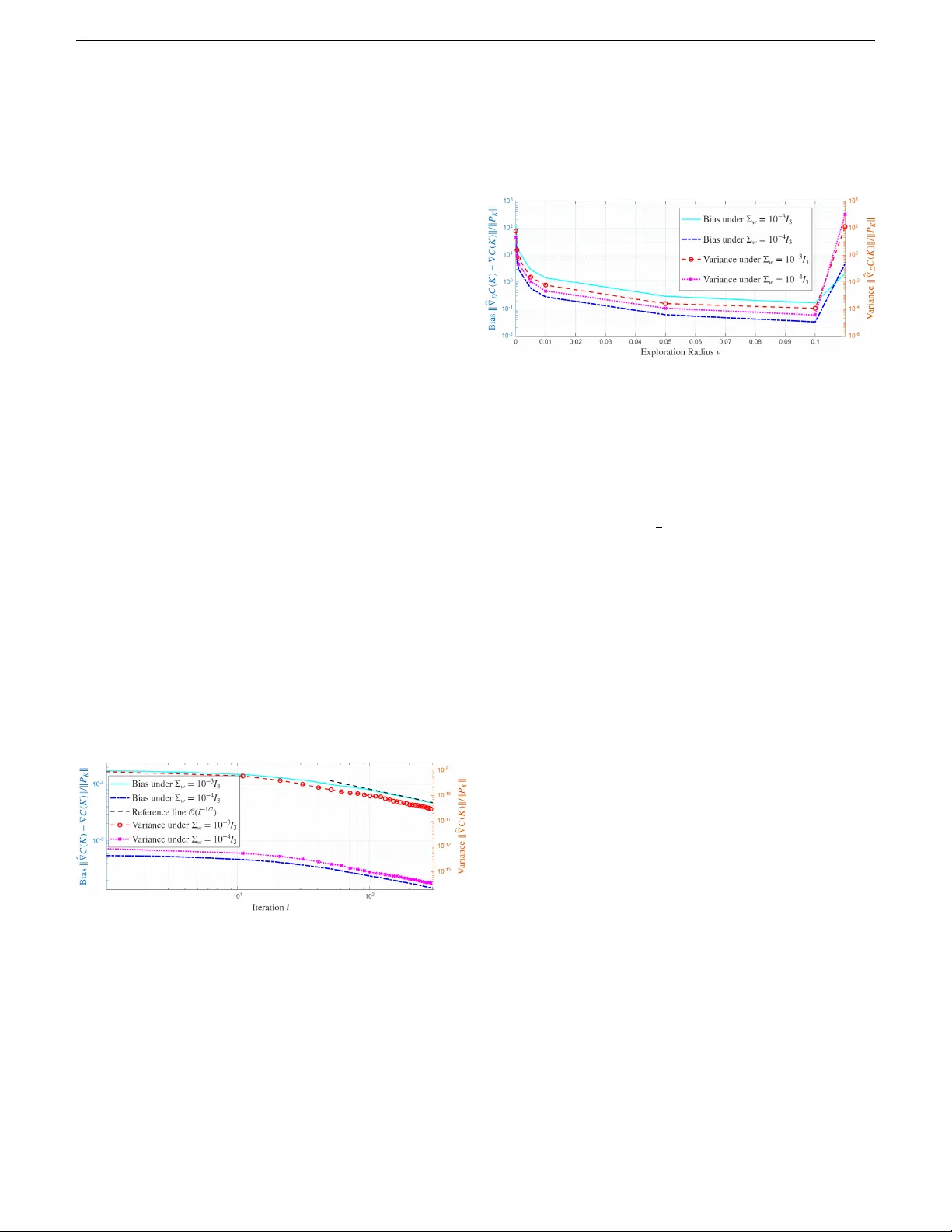
1 A Stochastic Gradient Descent Approach to Design P olicy Gradient Methods f or LQR Bow en Song, Simon W eissmann, Mathias Staudigl and Andrea Iannelli, Member , IEEE Abstract — In this work, we pr opose a stoc hastic gradient descent (SGD) framework to design data-driven policy gra- dient descent algorithms for the linear quadratic regulator prob lem. T wo alternative schemes are considered to esti- mate the policy gradient from stochastic trajectory data: (i) an indirect online identiﬁcation–based approach, in which the system matrices are ﬁrst estimated and subsequently used to construct the gradient, and (ii) a direct zeroth-or der approac h, which appro ximates the gradient using empirical cost evaluations. In both cases, the resulting gradient esti- mates are random due to stochasticity in the data, allowing us to use SGD theory to analyze the con vergence of the associated policy gradient methods. A key technical step consists of modeling the gradient estimates as suitable stochastic gradient oracles, which, because of the way the y are computed, are inherently based. W e derive sufﬁcient conditions under which SGD with a biased gradient or- acle conver ges asymptotically to the optimal policy , and leverage these conditions to design the parameters of the gradient estimation schemes. Moreover , we compare the adv antages and limitations of the two data-driven gradient estimators. Numerical experiments v alidate the effective- ness of the proposed methods. Index T erms — Stochastic Gradient Descent, P olicy Gra- dient Methods, Stoc hastic Appro ximation, Data-driven Con- trol I . I N T R O D U C T I O N R EINFORCEMENT learning (RL) [1] has had a profound impact across a wide range of applications [2], [3]. A central component of RL is policy optimization, in which a parameterized policy is directly optimized with respect to a prescribed performance objecti ve [4]. Among various policy optimization framework, this work focuses on policy gradient (PG) methods. Understanding the behavior of PG methods, particularly their conv ergence to the optimal polic y in the presence of uncertainty and stochastic disturbances, remains an activ e and important research direction [5], [6], and is essential for their reliable deployment in real-world applications [2], [3]. The linear quadratic regulator (LQR) problem has emerged as a canonical benchmark for studying RL in continuous state and action spaces due to its analytical tractability and practical Bowen Song acknowledges the suppor t of the International Max Planck Research School f or Intelligent Systems (IMPRS-IS). Bowen Song and Andrea Iannelli are afﬁliated with the Institute for Systems Theor y and Automatic Control, University of Stuttgar t, Ger- many (e-mail: bow en.song,andrea.iannelli@ist.uni-stuttgar t.de). Simon Weissmann and Mathias Staudigl are afﬁliated with the In- stitute for Mathematics, University of Mannheim, Ger man y (e-mail: simon.weissmann, mathias.staudigl@uni-mannheim.de). relev ance [7], [8]. PG methods have attracted substantial interest in this setting. A seminal result in [7] established global conv er gence of PG methods for deterministic LQR, which stimulated extensiv e follow-up works, such as [9]–[12]. These studies typically assume exact knowledge of the system dynamics and access to exact gradients. T o relax this assump- tion, more recent works such as [13], [14] analyze gradient- based methods under inexact gradients, providing valuable robustness insights. Howe ver , in these works, the gradient uncertainty is introduced through stylized perturbation models rather than arising naturally from data-driv en estimation. T o address gradient uncertainty arising from concrete esti- mation procedures rather than artiﬁcial perturbations, a promi- nent data-driv en approach is the indirect method, which fol- lows a two-step procedure: system dynamics are ﬁrst estimated from data, and PG methods are then applied using the es- timated model. Representative examples include [15], [16], which combine least-squares identiﬁcation with gradient-based updates under bounded noise assumptions. In contrast, direct data-driv en methods bypass explicit model identiﬁcation. One class of such methods estimates the quantities required for PG updates directly from data, with stochastic-setting examples giv en in [17], [18]. Another line of work studies direct PG methods based on data-driv en policy parameterizations, such as DeePC-based approaches [16], which typically operate under bounded-noise assumptions. While related, these direct data-driv en approaches are not the primary focus of this work. Another class of methods, closely related to the present study , employs zeroth-order techniques [19] in which gradients are approximated using noisy function ev aluations. This line of research originates from [7] in the deterministic LQR setting and has been extended to stochastic en vironments in [20] and [11], which consider inﬁnite- and ﬁnite-horizon problems, respectiv ely . These approaches rely on ergodic data collection and exploit the inherent robustness of PG methods, namely , that sufﬁciently accurate gradient estimates ensure cost contraction at each iteration. Howe ver , existing analyses are often conserv ative in two k ey respects: they typically require a large number of samples per iteration to control gradient estimation error , leading to high sample complexity , and they rely on uniform concentration guarantees enforced via union bounds, resulting in conﬁdence le vels that deteriorate exponentially with the number of iterations. T o reduce the conservati veness of prior analyses of zeroth- order methods, we propose here to incorporate stochastic gra- dient descent (SGD) [21], [22] into the analysis of PG methods 2 [23]. In SGD-based analyses, gradients are accessed through stochastic oracles, and con vergence is characterized using tools from stochastic approximation [24]–[26]. SGD has been shown to be effecti ve in both conv ex and non-conv ex settings [27], [28], including using zeroth-order optimization technique [29], [30]. While [22], [31] analyses assume unbiased gradient estimates, recent works [32], [33] extend the application of SGD theory with biased gradient oracles, providing a less restrictiv e modeling framework. For direct data-dri ven LQR, [34] ﬁrst adopted an SGD-style analysis under relativ ely strong assumptions on gradient estimation using zeroth-order meth- ods. Subsequent works [35], [36] relaxed these assumptions by employing alternativ e gradient estimation schemes, leading to improv ed sample efﬁcienc y and robustness. In [34]–[36], only a single gradient estimation scheme (zeroth-order method) is considered, and the analysis provides con ver gence guarantees only to a suboptimal solution. In this work, we leverage the SGD framework to design data-driv en policy gradient methods for solving the LQR problem in the presence of stochastic noise. W e employ two framew orks to estimate the gradient from noisy trajectory data: 1) Indirect method: Recursiv e least squares is used to estimate the system matrices, which are then used to compute a model-based gradient. 2) Direct method: A zeroth-order approach is employed to estimate the gradient directly from empirical cost ev aluations. Our main contributions are the following: 1) For both methods, we formalize the gradient estimates computed using stochastic trajectory data as gradient oracles with analytical characterizations of their ﬁrst and second moments. 2) Due to the nonlinear structure of the gradient, these oracles are inherently biased. Leveraging the gradient- dominated and quasi-smooth properties of the LQR cost function, we deri ve conditions on the step size and bias under which an SGD algorithm equipped with a general biased gradient oracle conv erges asymptotically to the optimal policy . Unlike classical SGD analyses on gradient-dominated functions [31], [37], [38], which as- sume L -smoothness, our results extend these guarantees to quasi-smooth functions. 3) Using the conditions deriv ed above, we design the parameters of both the indirect and direct gradient estimation schemes so that the resulting gradient oracles satisfy the required bias conditions. This, in turn, ensures that the corresponding data-dri ven policy gradient de- scent algorithms conv er ge asymptotically to the optimal policy . T o the best of the authors’ kno wledge, this is the ﬁrst work to demonstrate last iterate con vergence to the optimal policy across all data-driven policy gradient methods [7], [11], [15]–[18], [20], [34]–[36], whereas previous results typically guarantee con ver gence only to suboptimal solutions. Using the deriv ed conditions for con vergence, we analyze and compare the adv antages and limitations of the indirect and direct approaches. The paper is organized as follows. Section II introduces the problem setting and the necessary preliminaries. Section III describes the indirect and direct data-driv en polic y gradient estimation frameworks and formalizes them as gradient or- acles. Section IV in vestigates the con ver gence of SGD with biased gradient oracles for gradient-dominated and quasi- smooth cost functions. Section V analyzes and compares the indirect and direct data-driven policy gradient methods based on the conditions derived in the previous section. Section VI demonstrates the effecti veness of the proposed data-driv en policy gradient methods and shows numerical simulations. Finally , Section VII concludes the paper . Unless referenced otherwise, all the theoretical results are new . For readability , proofs can be found in the Appendix. Notations W e denote by A ⪰ 0 and A ≻ 0 a positi ve semideﬁnite and positiv e deﬁnite matrix A , respectiv ely . Z + and Z ++ are the sets of non-negati ve integers and positive integers. For matrices, ∥·∥ F and ∥·∥ denote respectiv ely their Frobenius norm and induced 2 -norm. A square matrix A is Schur stable if ρ ( A ) < 1 , where ρ ( A ) denotes its spectral radius. The symbols λ i ( A ) denote the smallest i -th eigenv alue of the square matrix A . I n and O n are the identity matrix and zero matrix with n row/columns, respecti vely . The symbols ⌊ x ⌋ and ⌈ x ⌉ denote the ﬂoor function, which returns the greatest integer smaller or equal than x ∈ R and ceil function, which returns the smallest integer greater or equal than x ∈ R , respectively . The indicator function is deﬁned as 1 A , for a measurable set A , deﬁned as 1 A ( w ) = 1 if w ∈ A and 1 A ( w ) = 0 if w / ∈ A . W e deﬁne the set B r ( K ) := { X ∈ R n x × n u |∥ K − X ∥ F < r } . A sequence is a map Z + → R n × m and is denoted by { Y t } , and its ﬁnite- horizon truncation up to index N is denoted by { Y t } N t =0 . For { Y t } , if the limit exists, we denote it by Y ∞ , i.e., Y t → Y ∞ as t → ∞ . For two positiv e scaler sequences { a t } and { g t } mapping Z + → R ≥ 0 , we denote a t = O ( g t ) if there exist constants C > 0 and t 0 such that a t ≤ C ( g ( t )) for all t ≥ t 0 and a t = o ( g t ) if lim t → + ∞ a t g t = 0 . I I . P R O B L E M S E T T I N G A N D P R E L I M I N A R I E S In this work, we consider the follo wing averaged inﬁnite- horizon optimal control problem, where the plant is subject to additiv e stochastic noise: min π ∈ Π lim T → + ∞ 1 T E x 0 ,w t T − 1 X t =0  x ⊤ t Qx t + u ⊤ t Ru t  , (1a) s . t . x t +1 = Ax t + B u t + w t , (1b) x 0 ∼ N (0 , Σ 0 ) , w t ∼ N (0 , Σ w ) , (1c) where A ∈ R n x × n x , B ∈ R n x × n u , ( A, B ) is stabilizable but unknown; cov ariance matrices Σ 0 , Σ x ≻ 0 ; Q, R ≻ 0 are the weight matrices. W e deﬁne the set of stabilizing feedback gains as: S :=  K ∈ R n u × n x   ρ ( A K ) ≤ 1  . (2) where A K := A + B K . The inﬁnite-horizon average cost under a linear policy u t = K x t with K ∈ S is giv en by: C ( K ) := lim T →∞ 1 T E x 0 ,w t " T − 1 X t =0 x ⊤ t Q K x t # , (3) B.SONG et al. : SGD T O DESIGN PGMS FOR LQR 3 with Q K := Q + K ⊤ RK . For any stabilizing policy K ∈ S , the gradient of the cost function C ( K ) is giv en by: ∇ C ( K ) = 2 E K Σ K , (4) where E K :=  R + B ⊤ P K B  K + B ⊤ P K A , P K is the solution to the L yapunov equation P K = A ⊤ K P K A K + Q K , and Σ K is the a verage covariance matrix associated with K ∈ S deﬁned as Σ K := lim T → + ∞ 1 T T − 1 X t =0 Σ t , with Σ t := E x 0 ,w t [ x t x ⊤ t ] . (5) It is a well-known fact [39] that the optimal K ∗ minimizing C satisﬁes K ∗ = − ( R + B ⊤ P K ∗ B ) − 1 B ⊤ P K ∗ A, (6a) P K ∗ = Q + A ⊤ P K ∗ A − A ⊤ P K ∗ B ( R + B ⊤ P K ∗ B ) − 1 B ⊤ P K ∗ A. (6b) Finally , deﬁne the le vel set S ( J ) with J ≥ C ( K ∗ ) as: S ( J ) :=  K ∈ R n x × n u   C ( K ) ≤ J  . (7) W e recall the boundedness of ∥∇ C ( K ) ∥ and ∥ K ∥ and local Lipschitz continuity properties of Σ K , C and ∇ C ov er the lev el set, which are used in the subsequent analysis. Lemma 1 (Boundedness of ∥∇ C ( K ) ∥ , ∥ K ∥ ): [7], [20, Proof of Lemmas 3/4] Gi ven any J 0 ≥ C ( K ∗ ) , for all K ∈ S ( J 0 ) , we have ∥∇ C ( K ) ∥ F ≤ b ∇ ( J 0 ) , (8a) ∥ K ∥ ≤ b K ( J 0 ) , (8b) where the expressions for b ∇ and b K are gi ven in (84) and (86) in Appendix IV, respectively . Lemma 2 (Lipschitz continuity of Σ K , C , ∇ C ): [7], [20, Lemmas 3/4/5] Suppose K ′ , K ∈ S are such that: ∥ K − K ′ ∥ ≤ h ( C ( K )) , (9) with h ( C ( K )) := λ 1 (Σ w ) λ 1 ( Q ) 4 C ( K ) ∥ B ∥ ( ∥ A ∥ + ∥ B ∥ b K ( C ( K ))+1) , it holds that: ∥ Σ K − Σ K ′ ∥ ≤ h Σ ( C ( K )) ∥ K − K ′ ∥ , (10) with h Σ ( C ( K )) := C ( K ) λ 1 ( Q ) h ( C ( K )) . If ∥ K − K ′ ∥ ≤ min { h ( C ( K )) , ∥ K ∗ ∥} , it holds that: ∥ C ( K ) − C ( K ′ ) ∥ ≤ h C ( C ( K )) ∥ K − K ′ ∥ , (11a) ∥∇ C ( K ) − ∇ C ( K ′ ) ∥ ≤ h ∇ ( C ( K )) ∥ K − K ′ ∥ . (11b) where h C , h ∇ are deﬁned in (88) and (87) in Appendix IV, respectiv ely . The cost function C (3) is non-con ve x but satisﬁes a beneﬁcial property known as gradient domination . Lemma 3 (Gradient Domination): [7], [20, Lemma 1] The function C on the set S is gradient dominated. That is, for any K ∈ S , the following inequality holds: C ( K ) − C ( K ∗ ) ≤ µ ∥∇ C ( K ) ∥ 2 F , (12) with µ := 1 4 ∥ Σ K ∗ ∥∥ Σ − 2 w ∥∥ R − 1 ∥ . In addition to gradient domination, the function C also satisﬁes a quasi-smoothness property . Lemma 4 (Quasi-smoothness): [7], [20, Lemmas 2/3] For any K ∈ S and perturbation K ′ satisfying ∥ K ′ − K ∥ F ≤ r ( C ( K )) , the cost function satisﬁes the following quasi- smoothness property:   C ( K ′ ) − C ( K ) − T r  ( K ′ − K ) ⊤ ∇ C ( K )    ≤ L ( C ( K )) 2 ∥ K ′ − K ∥ 2 F , (13) where L ( C ( K )) := 64 C ( K ) λ 1 ( Q ) λ 1 (Σ w ) ( ∥ B ∥ C ( K ) + λ 1 (Σ w ) ∥ R ∥ ) ; (14a) r ( C ( K )) := λ 1 ( Q ) 2 λ 1 (Σ w ) 2 32 ∥ B ∥ C ( K ) 2 (1 + ∥ A ∥ + ∥ B ∥ b K ( C ( K ))) . (14b) I I I . G R A D I E N T E S T I M A T I O N A N D G R A D I E N T O R A C L E S In this section, we study two data-dri ven approaches for estimating the policy gradient (4) when the system’ s model is unknown. The ﬁrst is an indirect method that identiﬁes the system matrices via recursive least squares, as described in Section III-A. The second is a zeroth-order method that approximates the gradient directly by using empirical cost ev aluations, discussed in Section III-B. In both cases, the gradient estimates, denoted in the following as ˆ ∇ C ( · ) are constructed from trajectory data generated by the stochastic system (1b), and thus inherit randomness from the data. Accordingly , these estimates can be viewed as stochastic gra- dients. Our objectiv e is to study their properties and formalize them as gradient oracles, which are characterizations of the gradient estimates through their ﬁrst and second moments. Concretely , for K ∈ S , we seek to provide for the indirect and direct estimators the following relationships: E [ ˆ ∇ C ( K )] = ∇ C ( K ) + ∆ b ( K ) , (15a) E  ∥ ˆ ∇ C ( K ) ∥ 2 F  ≤ c, (15b) where ∆ b is the bias term introduced by the estimation schemes; c is a uniform upper bound on the second moment of the gradient estimator . The existing literature [24], [31], [40] typically assumes that ∆ b ( K ) = 0 , an assumption that cannot be satisﬁed when gradients are estimated from data. A. Indirect Gradient Oracle In this subsection, we characterize the gradient oracle constructed from system matrix estimates obtained via the recursiv e least squares (RLS) algorithm. Let ˆ θ j := [ ˆ A j ˆ B j ] where ˆ A j and ˆ B j denote the RLS estimates at iteration j , and deﬁne the regressor data d j := [ x ⊤ j , u ⊤ j ] ⊤ obtained from trajectory . Giv en an initial estimate ˆ θ 0 and a matrix H 0 ≻ 0 , for all j ∈ Z + , the RLS updates are giv en by [41]: ˆ θ j = ˆ θ j − 1 + ( x j +1 − ˆ θ j − 1 d j ) d ⊤ j H − 1 j , (16a) H j = H j − 1 + d j d ⊤ j , (16b) The selection of ˆ θ 0 and H 0 will be speciﬁed later . The gradient at iteration j is computed using the online system estimates ˆ θ j (i.e. ˆ A j and ˆ B j ). Recall from Section II that for any K ∈ S , 4 the exact policy gradient is giv en by (4). Accordingly , the gradient constructed from the estimated model is gi ven by ˆ ∇ I C ( K , ˆ A j , ˆ B j ) = 2 ˆ E K ˆ Σ K , (17) where ˆ E K :=  R + ˆ B ⊤ j ˆ P K ˆ B j  K + ˆ B ⊤ j ˆ P K ˆ A j ; ˆ P K is the so- lution to the L yapunov equation ˆ P K = ( ˆ A j + ˆ B j K ) ⊤ ˆ P K ( ˆ A j + ˆ B j K ) + Q K ; ˆ Σ K is the solution to the L yapunov equation ˆ Σ K = ( ˆ A j + ˆ B j K ) ˆ Σ K ( ˆ A j + ˆ B j K ) ⊤ + Σ w . It is crucial to quantify how the estimation errors propagate into the gradient computation. T o this end, we consider generic estimates ˆ A and ˆ B (with a slight abuse of notation, suppressing the iteration index for clarity) and analyze the discrepancy between the true gradient and its estimated counterpart. W e now introduce the follo wing lemma to quantify the error in the estimated gradient induced by the model estimation error ∆ θ := [ ˆ A − A, ˆ B − B ] . Lemma 5 (Estimation Err or of Gradient): Given K ∈ S , if ∥ ∆ θ ∥ ≤ p θ , we have ∥ ˆ ∇ I C ( K , ˆ A, ˆ B ) − ∇ C ( K ) ∥ ≤ p ( C ( K ) , p θ ) ∥ ∆ θ ∥ , (18) where p θ and p are deﬁned in the proof (see (65) and (64) respectiv ely). The resulting indirect gradient estimation scheme based on RLS is summarized in Algorithm 1. The initialization of ˆ θ 0 and H 0 is speciﬁed in the ﬁrst stage of the algorithm, while the selection of the initial data length t 0 is discussed later . The excitation gain K j from sequence { K j } used for data generation in Algorithm 1 does not need to coincide with the gain K at which the gradient is ev aluated. When K j = K, ∀ j ∈ Z + , this is an on-policy estimation scheme; otherwise, it is an off-policy scheme. Algorithm 1 Indirect Data-driv en Gradient Estimation. Require: K ∈ S (gain at which the gradient is ev aluated); excitation gain { K j } ; e j ∈ N (0 , Σ e ) ; number of iteration n ∈ Z + . for t = 1 , ..., t 0 do (initialization) Apply control input u t = K 0 x t + e t Collect data [ x t , u t , x t +1 ] Set H 0 = P t 0 t =1 [ d t d ⊤ t ] and ˆ θ 0 = P t 0 t =1 [ x t +1 d ⊤ t ] H − 1 0 for j = 1 , ..., n do (iteration counter) Apply control input: u j + t 0 = K j x j + t 0 + e j + t 0 (19) Collect data [ x j + t 0 , u j + t 0 , x j +1+ t 0 ] Update ( ˆ θ j , H j ) using the RLS recursion (16) Extract system estimates ˆ A n , ˆ B n ← ˆ θ n Compute gradient estimate ˆ ∇ I C ( K , ˆ A n , ˆ B n ) using (17) At each iteration, the gradient is ev aluated using the current system matrix estimates constructed from all previously col- lected data. As the iteration number n increases, the estimator and consequently the gradient lev erage an expanding dataset, leading to progressi vely improv ed accuracy . The estimated system matrices from Algorithm 1 can be expressed as: ˆ θ n =  n + t 0 X k =1 x k +1 d ⊤ k  n + t 0 X k =1 d k d ⊤ k  − 1 , ∀ n ∈ Z + . (20) Then, the corresponding estimation error ∆ θ n := [ ˆ A n − A ˆ B n − B ] is given by: ∆ θ n =  n + t 0 X k =1 w k d ⊤ k  n + t 0 X k =1 d k d ⊤ k  − 1 , ∀ n ∈ Z + . (21) Quantifying the estimation error of the RLS procedure is crucial to later characterize the gradient estimates as suitable gradient oracles. A key factor governing the accuracy of the estimates is the informativity of the data, which is commonly formalized through the notion of persistency of excitation . W e next recall the deﬁnition of local persistency . Deﬁnition 1 (Local P ersistency): [42, Deﬁnition 2] A ﬁ- nite horizon sequence { d j } n j =0 is locally persistent with re- spect to N , M , α , if n ≥ max { M , N } and there exist N ≥ 1 , M ≥ 1 and α > 0 , such that for all j = M q + 1 where q ∈ [0 , ..., ⌊ n max { N ,M } ⌋ − 1] , N − 1 X k =0 d j + k d ⊤ j + k ⪰ αI n x + n u . (22) Beyond the informati vity of the data, the analysis of the estimation error also necessitates establishing the boundedness of the data sequence. W e present the following lemma, which establishes the mean-squar e boundedness of the stochastic system under a con vergent stabilizing gain sequence { K j } . Lemma 6 (Mean-squar e Boundedness): Suppose that the excitation gain sequence { K j } conv erges to K ∞ , where the limiting closed-loop matrix A K ∞ is Schur stable. Then, for any n ∈ Z + , the state sequence { x j } n + t 0 j =1 generated by Algorithm 1 is mean-square bounded; namely , there exists a constant ¯ x > 0 , independent of n , such that sup 1 ≤ j ≤ n + t 0 E [ ∥ x j ∥ 2 ] ≤ ¯ x, ∀ n ∈ Z + . (23) W e are now ready to present a theorem that analyzes the estimation error of RLS in the presence of stochastic noise. Theorem 1. Assume that the data sequence { d j } n + t 0 j =1 generated by Algorithm 1 is locally persistent with parameters N 0 , M 0 , α 0 . Suppose further that t 0 ≥ max { N 0 , M 0 } and that the contr ol gain sequence { K j } con verg es to K ∞ , wher e the limiting closed-loop matrix A K ∞ is Schur stable. Deﬁne ¯ K := sup j ∈ N ∥ K j ∥ . Then, for any n ∈ Z + , the estimation err or of system matrices fr om Algorithm 1 satisﬁes: E [ ∥ ∆ θ n ∥ ] ≤ s c x max { N 0 , M 0 } 2 α 2 0 ( n + t 0 ) = O ( 1 √ n ) , (24) wher e c x := T r(Σ w )[(1 + ∥ ¯ K ∥ 2 ) ¯ x + T r(Σ e )]; (25) and ¯ x is intr oduced in (23) . Moreo ver , for any pr escribed bound β > 0 , if the initial data length t 0 satisﬁes t 0 ≥ max n c x max { N 0 ,M 0 } 2 α 2 0 β 2 , N 0 , M 0 o , then ∀ n ∈ Z + P  ∥ ∆ θ n ∥ ≤ β  ≥ 1 − s c x max { N 0 , M 0 } 2 β 2 α 2 0 t 0 . (26) Theorem 1 implies that, provided suf ﬁciently informati ve data are collected, which can be ensured by an appropriate choice of the dithering input sequence { e j } , the expected B.SONG et al. : SGD T O DESIGN PGMS FOR LQR 5 estimation error can be made arbitrarily small with probabil- ity . Having characterized the estimation error of the system matrices (Theorem 1) and the corresponding gradient error (Lemma 5), we are now ready to formalize the gradient oracle for the indirect method from Algorithm 1. Lemma 7 (Gradient Oracle fr om Indirect Method): Consider the gradient estimates by Algorithm 1. Assume that the data sequence { d j } n + t 0 j =1 generated in Algorithm 1 is locally persistent with parameters N 0 , M 0 , α 0 , and that the excitation gain sequence { K j } conv erges to K ∞ , where the limiting closed-loop matrix A K ∞ is Schur stable. Deﬁne ¯ K := sup j ∈ N ∥ K j ∥ . For t 0 ≥ max n c x max { N 0 ,M 0 } 2 α 2 0 p 2 θ , N 0 , M 0 o and all n ∈ Z + , with probability at least 1 − q c x max { N 0 ,M 0 } 2 p 2 θ α 2 0 t 0 , we hav e ∥ ∆ θ n ∥ ≤ p θ , where c x is deﬁned in (25). Then for any K ∈ S and n ∈ Z + , the gradient estimator satisﬁes the following properties: E h ˆ ∇ I C ( K , ˆ A n , ˆ B n ) i = ∇ C ( K ) + ∆ I ( K, E [∆ θ n ]) , (27a) E h ∥ ˆ ∇ I C ( K , ˆ A n , ˆ B n ) ∥ 2 F i ≤ V I ( C ( K ) , p ( C ( K ) , p θ )) , (27b) where ∆ I ( K, E [∆ θ n ]) := E [ ˆ ∇ I C ( K , ˆ A n , ˆ B n ) − ∇ C ( K ) | K ] ; ∥ ∆ I ( K, E [∆ θ n ])] ∥ ≤ ¯ ∆ I ( C ( K ) , E [ ∥ ∆ θ n ∥ ]); (28) and ¯ ∆ I ( C ( K ) , E [ ∥ ∆ θ n ∥ ]) := p ( C ( K ) , p θ ) E [ ∥ ∆ θ n ∥ ] ; V I is deﬁned in (69). Lemma 7 sho ws that the gradient estimates produced by Algorithm 1 are generally biased (27a), and that their second moment (27b) bound also depends on the estimation error . Recalling the deﬁnition of the gradient oracle (15), Lemma 7, provides an explicit characterization of the gradient estimates arising from the indirect method as a biased oracle. Combining Theorem 1 with Lemma 7, we observe that the norm of the bias term decays at a rate of O ( n − 1 / 2 ) . B. Direct Gradient Oracle In this subsection, we in vestigate the gradient oracle ob- tained from the direct method, which we refer to as the zeroth- order method (Z.O.M). For this, we introduce a smoothing function deﬁned as: C v ( K ) := E U ∼ B v [ C ( K + U ) U ] , ∀ K ∈ S , (29) where B v denotes the uniform distribution over all matrices of size n u × n x with Frobenius norm less than the smoothing radius v . It is shown in [7] that the gradient of the smoothed function satisﬁes: ∇ C v ( K ) = E U ∼ B v [ ∇ C ( K + U )] = n x n u v 2 E U ∼ S v [ C ( K + U ) U ] , (30) where S v denotes the uniform distribution over the boundary of the Frobenius norm ball with radius v . The algorithm used to estimate the gradient is presented in Algorithm 2. The Algorithm 2 Direct Data-driv en Gradient Estimation Require: Gain matrix K ∈ S , number of rollouts n , rollout length ℓ , exploration radius v ; for k = 1 , ..., n do 1. Generate a sample gain matrix ¯ K k = K + U k , where U k is drawn uniformly at random ov er matrices of compatible dimensions with radius v ; 2. Generate an initial state x ( k ) 0 with x ( k ) 0 ∼ (0 , Σ 0 ) ; 3. Excite the closed-loop system with: u ( k ) t = ¯ K k x ( k ) t (31) for ℓ -steps starting from x ( k ) 0 , yielding the state sequence n x ( k ) t o ℓ − 1 t =0 originating from (1); 4. Collect the empirical cost estimate ˆ C ¯ K k := 1 ℓ P ℓ − 1 t =0 x ( k ) ⊤ t ( Q + ¯ K ⊤ k R ¯ K k ) x ( k ) t ; Gradient estimate ˆ ∇ D C ( K , v , ℓ, n ) := 1 n P n k =1 n x n u v 2 ˆ C ¯ K k U k . empirical gradient estimator in Algorithm 2 is gi ven by: ˆ ∇ D C ( K , v , ℓ, n ) = 1 n n X k =1 n x n u v 1 ℓ ℓ − 1 X t =0 x ( k ) ⊤ t Q K k x ( k ) t ! U k . (32) W e now characterize the gradient oracle associated with (32). Lemma 8 (Gradient Oracle fr om Direct Method): Giv en K ∈ S , if the exploration radius v satisﬁes the following condition: v ≤ min { h ( C ( K )) , ∥ K ∗ ∥} , (33) where h ( · ) is deﬁned in Lemma 2, then the gradient estimates from Algorithm 2 satisfy the following properties: E [ ˆ ∇ D C ( K , v , ℓ, n )] = ∇ C ( K ) + ∆ D ( K, v , ℓ ) , (34a) E  ∥ ˆ ∇ D C ( K , v , ℓ, n ) ∥ 2 F  ≤ V D ( C ( K ) , v , ℓ, n ) , (34b) where ∆ D ( K, v , ℓ ) := E [ ˆ ∇ D C ( K , v , ℓ, n ) − ∇ C ( K ) | K ] and ∥ ∆ D ( K, v , ℓ ) ∥ F ≤ ¯ ∆ D ( C ( K ) , v , ℓ ) . (35) ¯ ∆ D and V D are deﬁned in (72) and (73) and satisfy: ¯ ∆ D ( C ( K ) , v , ℓ ) = O  1 v ℓ + v  , (36a) V D ( C ( K ) , v , ℓ, n ) = O  1 + 1 nℓv 2 + 1 nv 2  . (36b) Lemma 8 characterizes the gradient oracle (15) for the direct method by establishing its ﬁrst and second moments. Similar to [7], [20], the gradient estimation error depends on three key parameters: ℓ , v , and n . The choice of ( ℓ, v ) is critical for controlling both the bias and v ariance of the gradient estimates. The number of samples, n , only inﬂuences the variance of the estimator; speciﬁcally , a larger n leads to a smaller second moment. I V . C O N V E R G E N C E A N A L Y S I S O F S G D W I T H B I A S E D G R A D I E N T In the previous section, we showed that the gradients generated by the two considered estimators can be modeled as 6 gradient oracles. Inspection of their e xpressions re veals that the gradient estimators are biased. In this section, we analyze the con vergence of stochastic gradient descent applied to gr adient- dominated and quasi-smooth functions in the presence of biased gradient oracles. W e perform the stochastic gradient descent update: K i +1 = K i − η i ˆ ∇ C ( K i ) , ∀ i ∈ Z + , (37) where ˆ ∇ C ( K i ) is a stochastic gradient obtained from a suit- able estimator, speciﬁcally one of the two concrete algorithms introduced in Section III. From Lemmas 7 and 8, ∀ i ∈ Z + , giv en an iterate K i from (37), both indirect and direct oracles satisfy the following properties almost surely (a.s.): E [ ˆ ∇ C ( K i ) | K i ] = ∇ C ( K i ) + ∆( K i , i ) , (38a) E  ∥ ˆ ∇ C ( K i ) ∥ 2 F   K i ] ≤ c, (38b) where the bias term satisﬁes: ∥ ∆( K i , i ) ∥ F ≤ ¯ ∆( C ( K i )) , ∀ i ∈ Z + , (39) and the function ¯ ∆( C ( K )) decreases monotonically as the cost C ( K ) decreases. W e provide the following explanations for the bias term as well as for the boundedness of the second moment. 1) the term ∆( K i , i ) denotes the iteration-dependent bias introduced either by the model estimates ˆ A i , ˆ B i at i - th iteration (as discussed in Section III-A) or by the exploration radius v i , and the ﬁnite rollout length ℓ i (as discussed in Section III-B). This bias may v ary across iterations. In the indirect setting, it ev olves together with the model-learning process, whereas in the zeroth-order method it may arise from the iteration-varying choices of v i and ℓ i . Because quantifying the bias term ∆( K i , i ) is challenging, our analysis focuses on bounding its norm ∥ ∆( K i , i ) ∥ F (as in Lemma 7 and Lemma 8). 2) In the SGD literature [24], [40], the second moment is often assumed to satisfy the following ABC con- dition: E  ∥ ˆ ∇ C ( K ) ∥ 2 F   K ≤ a ( C ( K ) − C ( K ∗ )) + b ∥∇ C ( K ) ∥ 2 + c . W e assume a uniform second-moment bound, i.e., a = b = 0 , instead of the more general ABC condition, because in the subsequent analysis, we show that such a bound can indeed be established for the proposed gradient estimators over a local level set. The following assumption plays a crucial role for studying the con vergence of (37) to the optimal solution. Assumption 1: The bias term ∥ ∆( K i , i ) ∥ F decays at least as O ( 1 i β ) for some β ≥ 1 2 . This assumption can be satisﬁed by appropriately choosing the parameters in the gradient estimation process for both methods. A detailed discussion is provided in Section V. Before proceeding with the con ver gence analysis, we ﬁrst introduce the following two lemmas. Lemma 9: Consider a sequence { K i } generated by the update rule in (37), initialized at K 0 ∈ S with step size sequence { η i } . T ake J 0 > 0 satisfying C ( K 0 ) ≤ J 0 . Deﬁne the event C as: C :=  K k ∈ B r ( J 0 ) ( K k − 1 ) , ∀ k ∈ Z ++  , (40) where r ( · ) is deﬁned in (14b). Giv en δ ∈ (0 , 1) , and the step sizes { η i } satisfy the following condition: ∞ X k =1 η 2 k ≤ r 2 ( J 0 ) δ c . (41) Then the ev ent C occurs with probability at least 1 − δ . Lemma 10: Consider a sequence { K i } generated by (37), initialized at K 0 ∈ S with step size sequence { η i } . T ake J 0 > 0 satisfying J 0 > C ( K 0 ) , and choose δ 1 , δ 2 , and δ 3 ∈ (0 , 1) such that δ = 1 − (1 − δ 1 − δ 2 )(1 − δ 3 ) ∈ (0 , 1) . Deﬁne ϵ := ( √ 1+4 ϵ ′ 2 − 1 2 ) 2 with ϵ ′ := J 0 − C ( K 0 ) > 0 and the ev ent: Ω := { K i ∈ S ( J 0 ) , ∀ i ∈ Z + } , (42) where S ( · ) is deﬁned in (7). Suppose Assumption 1 and the following conditions on the step sizes hold: 1) The step size sequence { η i } satisﬁes η i < µ, ∀ i ∈ Z + , (43) where µ is deﬁned in (12). 2) The step sizes are chosen as η i = O  1 i κ  for some κ ∈  1 2 , 1  and sufﬁciently small so that ∞ X i =1 η 2 i ≤ δ 1 ϵ α 1 ( J 0 , ¯ ∆( J 0 )) + c , (44) where α 1 is polynomial function deﬁned as: α 1 ( J 0 , ¯ ∆( J 0 )) := n u cb ∇ ( J 0 ) 2 + 3 b ∇ ( J 0 ) 4 + 2 n u b ∇ ( J 0 ) 3 ¯ ∆( J 0 ) . (45) with ¯ ∆ and b ∇ as deﬁned in (39) and Lemma 1. 3) The step sizes further satisfy: ∞ X i =0 η i ∥ ∆( K i , i ) ∥ F ≤ s δ 2 ϵ n 3 u b ∇ ( J 0 ) 2 . 4) The step sizes condition in Lemma 9 with δ = δ 3 holds: ∞ X i =1 η 2 i ≤ r 2 ( J 0 ) δ 3 c . (46) Then, the ev ent F := C ∩ Ω (47) occurs with probability at least 1 − δ . After establishing Lemma 10, we can lev erage the quasi- smoothness property in Lemma 4 to conclude that C is L ( J 0 ) - smooth ov er the level set S ( J 0 ) . On the event C , Lemma 4 can be applied to analyze con ver gence in the stochastic setting. Now , we can lev erage the Robbins–Siegmund theorem [26] to analyze the conv ergence of the SGD algorithm for the gradient-dominated and quasi-smooth LQR cost function C in the presence of a biased gradient oracle. Theorem 2. Consider a sequence { K i } generated by (37) , initialized at K 0 ∈ S with step size sequence { η i } . Using the same deﬁnitions of J 0 , ϵ , ϵ ′ , δ , δ 1 , δ 2 , and δ 3 as in Lemma 10, that is, let J 0 > 0 satisfy J 0 > C ( K 0 ) and choose δ 1 , δ 2 , and δ 3 ∈ (0 , 1) such that δ = 1 − (1 − δ 1 − δ 2 )(1 − δ 3 ) ∈ (0 , 1) . Deﬁne ϵ := ( √ 1+4 ϵ ′ 2 − 1 2 ) 2 with ϵ ′ := J 0 − C ( K 0 ) > 0 . B.SONG et al. : SGD T O DESIGN PGMS FOR LQR 7 Suppose that Assumption 1 holds and step sizes η i = O  1 i κ  for some κ ∈  1 2 , 1  . Further assume that { η i } is chosen sufﬁciently small such that the following conditions hold: η i < µ, ∀ i ∈ Z + ; (48a) ∞ X i =1 η 2 i ≤ min  δ 1 ϵ α 1 ( J 0 , ¯ ∆( J 0 )) + c , r 2 ( J 0 ) δ 3 c  ; (48b) ∞ X i =0 η i ∥ ∆( K i , i ) ∥ F ≤ s δ 2 ϵ n 3 u b ∇ ( J 0 ) 2 , (48c) wher e µ is deﬁned in (12) , r ( · ) is the local radius fr om (14b) , and α 1 is the polynomial function deﬁned in (45) . Then, the event F has pr obability at least 1 − δ . Moreo ver , for any λ ∈ (2 − 2 κ, 1) , the following holds: 1) ( C ( K i ) − C ( K ∗ )) 1 F = o  1 i 1 − λ  , a.s.; 2) E [( C ( K i ) − C ( K ∗ )) 1 F ] = o  1 i 1 − λ  . The following observations are in order: 1) Theorem 1 establishes that, under appropriate conditions on the step size and the magnitude of the bias term, the sequence { C ( K i ) } conv erges asymptotically to the optimal function v alue C ( K ∗ ) both in expectation and for almost all sequence realizations (almost surely), when the ev ent F happens. 2) Under Assumption 1 and with the step-size sequence η i = O ( i − κ ) , the bias-related term P ∞ i =0 η i ∥ ∆( K i , i ) ∥ F is absolutely summable. The step size magnitude is chosen based on (48c) to ensure the desired conﬁdence lev el δ 2 and ϵ . V . C L O S I N G T H E L O O P B E T W E E N S G D A N D G R A D I E N T E S T I M A T O R S In the previous section, we analyzed the con ver gence of SGD applied to the LQR policy gradient problem with the generic gradient oracle (38). The analysis helped us identify sufﬁcient conditions on stepsize choices and gradient accuracy under which SGD conv erges to the optimal cost. W e now show ho w tuning parameters of the two gradient estimators presented in Section III can be chosen to satisfy these condi- tions. The block diagram corresponding to the two data-driv en policy gradient algorithms is illustrated in Figure 1. A. Indirect Methods The method is built upon Algorithm 1. At each iteration i , the system estimates ˆ θ i , produced by Algorithm 1, are used to construct the gradient associated with the current policy K i , followed by a policy gradient descent step (37). After applying the control input (19), new data are collected and subsequently lev eraged to update the estimates of the system matrices ˆ θ i +1 . W e emphasize that, within the indirect framework, the excitation gain in (19) does not need to be on-policy , as illustrated in Figure 1. In particular , the system can be operated using a ﬁxed stabilizing gain K , corresponding to an off-policy setting. A detailed discussion on the distinction between off- policy and on-policy schemes is provided in Remark 1. The follo wing theorem establishes con ver gence guarantees to the optimal solution using the indirect data-dri ven policy gradient algorithm based on Algorithm 1. Linear System x t +1 = Ax t + B u t + w t Con troller (19) for Indirect (31) for Direct P olicy Gradient Descent K i +1 = K i − η i ˆ ∇ C ( K i ) Gradien t Estimator Indirect : Algorithm 1 Direct : Algorithm 2 { x t } { u t } { ˆ ∇ C ( K i ) } { K i } Fig. 1. Data-dr iv en policy gradient descent framework Theorem 3. Consider the indir ect data-driven policy gradient algorithm based on Algorithm 1, generating a sequence { K i } via (37) , initialized at K 0 ∈ S with step-size sequence { η i } . Using the same deﬁnitions of J 0 , ϵ , ϵ ′ , δ , δ 1 , δ 2 , and δ 3 as in Theor em 2, that is, let J 0 > 0 satisfy J 0 > C ( K 0 ) and choose δ 1 , δ 2 , and δ 3 ∈ (0 , 1) such that δ = 1 − (1 − δ 1 − δ 2 )(1 − δ 3 ) ∈ (0 , 1) . Deﬁne ϵ := ( √ 1+4 ϵ ′ 2 − 1 2 ) 2 with ϵ ′ := J 0 − C ( K 0 ) > 0 . Assume that the data sequence { d i } is locally per sistent with parameters N 0 , M 0 , α 0 . Given a t 0 intr oduced in Algorithm 1 satisfying: t 0 ≥ max  M 0 , N 0 , c x max { N 0 , M 0 } 2 p ′ θ ( J 0 ) 2 α 2 0  , (49) wher e p ′ θ and c x ar e deﬁned in (83) and (25) , r espectively . Then with pr obability at least 1 − q c x max { N 0 ,M 0 } 2 p ′ θ ( J 0 ) 2 α 2 0 t 0 , the bias term of the gradient oracle satisﬁes: ∥ ∆ I ( K i , E [∆ θ i ])] ∥ F ≤ c d E [ ∥ ∆ θ i ∥ ] = O ( 1 i 1 / 2 ) , (50) wher e c d := max { n x , n u } p ( J 0 , p ′ θ ( J 0 )) and p was deﬁned in (64) . Additionally , consider the step sizes of the form η i = O ( 1 i κ ) for some κ ∈  1 2 , 1  . Further , suppose the step sizes satisfy: η i < µ, ∀ i ∈ Z + ; (51a) ∞ X i =1 η 2 i ≤ max  δ 1 ϵ α 1 ( J 0 , ¯ ∆( J 0 )) + c , r 2 ( J 0 ) δ 3 V I ( J 0 , p ( J 0 , p ′ θ ( J 0 )))  ; (51b) ∞ X i =0 η i c d s c x max { N 0 , M 0 } 2 α 2 0 ( i + t 0 ) ≤ s δ 2 ϵ n 3 u b ∇ ( J 0 ) 2 . (51c) Then, the event F occurs with pr obability at least (1 − δ )  1 − q c x max { N 0 ,M 0 } 2 p ′ θ ( J 0 ) 2 α 2 0 t 0  . Mor eover , for any λ ∈ (2 − 2 κ, 1) , the following holds: 1) ( C ( K i ) − C ( K ∗ )) 1 F = o  i − (1 − λ )  , a.s.; 2) E [( C ( K i ) − C ( K ∗ )) 1 F ] = o  i − (1 − λ )  . 8 The proof combines the main results of Theorem 2 and Lemma 7. The key step is to v erify that the bias term appearing in the gradient oracle decays at an appropriate rate. Under the local persistence assumption, the expected estimation error in the indirect method decreases at the rate O ( i − 1 / 2 ) , which matches the requirement for con ver gence of SGD with a biased gradient oracle. Moreover , a uniform upper bound on the second-moment term can always be established as V I ( b K ( J 0 ) , p ( b K ( J 0 ) , p ′ θ ( J 0 ))) . Consequently , with a properly chosen step size, the indirect method con ver ges asymptotically to the optimal polic y without requiring any modiﬁcation to the underlying indirect gradient estimation algorithm based on recursive least-squares. Remark 1: From Theorem 3, the parameter c x (deﬁned in (25)), which depends on ¯ x introduced in (23), plays a critical role in the conv ergence analysis. In the on-policy setting, where the system is excited using the policies generated by the policy gradient updates, we can only guarantee the existence of such a bound. This is because, with high probability , each gain { K i } , i ∈ Z + , stabilizes the system and the sequence { K i } con ver ges asymptotically to K ∗ . Howe ver , the value of c x depends on the stochastic policy sequence { K i } , and a closed-form expression is generally unavailable. In contrast, in the off-policy setting, where the system is excited using a ﬁxed stabilizing gain K rather than the iterates { K i } generated by the SGD algorithm, an explicit bound on c x can be com- puted directly . This enables a more precise characterization of c x and, in turn, leads to sharper bounds on the bias and con vergence behavior under off-policy data collection. B. Direct Methods The direct data-dri ven policy gradient method proceeds as follows. At each iteration, Algorithm 2 is used to estimate the gradient. W e let the parameters v i , ℓ i , and n i in Algorithm 2 vary across the iterations to control the bias and variance. The estimated gradient is then applied in a policy gradient descent step. In the direct method, only an on-policy scheme can be employed.The following theorem establishes conv ergence guarantees to the optimal solution using the direct data-driven policy gradient Algorithm. Theorem 4. Consider the dir ect data-driven policy gradient algorithm based on Algorithm 2, generating a sequence { K i } via (37) , initialized at K 0 ∈ Z + with step-size sequence { η i } . Using the same deﬁnitions of J 0 , ϵ , ϵ ′ , δ , δ 1 , δ 2 , and δ 3 as in Theor em 2, that is, let J 0 > 0 satisfy J 0 > C ( K 0 ) and choose δ 1 , δ 2 , and δ 3 ∈ (0 , 1) such that δ = 1 − (1 − δ 1 − δ 2 )(1 − δ 3 ) ∈ (0 , 1) . Deﬁne ϵ := ( √ 1+4 ϵ ′ 2 − 1 2 ) 2 with ϵ ′ := J 0 − C ( K 0 ) > 0 . Assume that the parameters of the Algorithm 2 satisfy: v i ≤ min { h ( J 0 ) , | K ∗ ∥} , ∀ i ∈ Z + , (52a) v i = O ( 1 i 1 / 2 ) , ℓ i = O ( i ) , n i = O ( i ) . (52b) Then, the bias term of the gradient oracle and the second moment satisfy: ¯ ∆ D ( C ( K i ) , v i , ℓ i ) ≤ ¯ ∆ D ( J 0 , v i , ℓ i ) = O ( 1 i 1 / 2 ) , (53a) V D ( C ( K ) , v i , ℓ i , n i ) ≤ sup i V D ( J 0 , v i , ℓ i , n i ) =: ¯ V D . (53b) Additionally , consider the step sizes of the form η i = O ( 1 i κ ) for some κ ∈  1 2 , 1  . Further , suppose the step sizes satisfy: η i < µ, ∀ i ∈ Z + ; (54a) ∞ X i =1 η 2 i ≤ min  δ 1 ϵ α 1 ( J 0 , ¯ ∆( J 0 )) + c, , r 2 ( J 0 ) δ 3 ¯ V D  ; (54b) ∞ X i =0 η i ¯ ∆ D ( J 0 , v i , ℓ i ) ≤ s δ 2 ϵ n 3 u b ∇ ( J 0 ) 2 . (54c) Then, the event F occurs with pr obability at least (1 − δ ) . Mor eover , for any λ ∈ (2 − 2 κ, 1) , the following holds: 1) ( C ( K i ) − C ( K ∗ )) 1 F = o  i − (1 − λ )  , a.s.; 2) E [( C ( K i ) − C ( K ∗ )) 1 F ] = o  i − (1 − λ )  . The proof of Theorem 4 follows from Theorem 1 and Lemma 8 by designing the parameters r i , n i , and ℓ i such that the resulting gradient oracle satisﬁes the required bias decay and bounded-v ariance conditions. T o guarantee con vergence to the optimal policy , the exploration radius v i must decrease and the rollout length ℓ i must increase so that the bias term vanishes at the required rate. Ne vertheless, a smaller v i leads to an inﬂation of the variance, which necessitates increasing the number of rollouts n i to maintain a bounded second moment. C . Comparison between the two gradient estimators T o guarantee con vergence to the optimal policy , the indirect and direct policy gradient methods differ in the following aspects, as characterized in Theorems 3 and 4: • Sample Comple xity: the indirect and direct policy gradient methods impose fundamentally different sample require- ments. The indirect method updates the system estimates using all previously collected data and requires only O (1) new samples per iteration to achieve the desired bias decay . In contrast, the direct method relies solely on empirical cost e valuations at the current iterate and cannot reuse past data, resulting in a per-iteration sample com- plexity of O ( i 2 ) . This disparity reﬂects the inherent bias and variance trade-off in zeroth-order gradient estimation, implying that direct methods require substantially more data than indirect methods to achiev e conv ergence to the optimal policy . • Excitation P olicy: For the indirect method, conv ergence to the optimal policy requires the data sequence { d i } to satisfy the local persistency condition deﬁned in Deﬁni- tion 1. T o this end, the dithering signal { e i } is introduced in (19). The excitation gain in the indirect framework may be either of f-policy or on-policy , as discussed in Remark 1. In contrast, for the direct method, the gradient is approximated via the smoothing function (29), where a random perturbation matrix U is introduced in the gain, leading to the control input format in (31). In this case, only an on-policy implementation is possible. • Data Collection: In the indirect method, online data are continuously used to update the system estimates, and the gradient is computed based on the updated estimates. For the direct method, data are collected via independent ﬁnite-horizon rollouts; that is, the state is re-initialized at x ( k ) 0 for each trajectory , as speciﬁed in Algorithm 2. B.SONG et al. : SGD T O DESIGN PGMS FOR LQR 9 • Initial Data Collection Phase: A limitation of the indirect method is that its conv ergence guarantees rely on an initial data collection phase to ensure that the system ma- trix estimates are sufﬁciently close to the true dynamics. In contrast, the direct method does not require such an initialization phase. V I . N U M E R I C S In this section, we present numerical simulation results 1 to illustrate and validate the theoretical ﬁndings dev eloped in the previous sections. A. Gradient Oracle Analysis In this subsection, we in vestigate how dif ferent factors af fect the behavior of the gradient oracle, as discussed in Section III. W e consider the following benchmark linear system, which has been widely used in prior studies [17]. The system dynamics are given by x t +1 =   1 . 01 0 . 01 0 0 . 01 1 . 01 0 . 01 0 0 . 01 1 . 01   x t +   1 0 0 0 1 0 0 0 1   u t + w t . (55) The weight matrices Q and R are chosen as 0 . 001 I 3 and I 3 . The initial cov ariance matrix Σ 0 = 10 − 1 I 3 . The gain K , for which we want to e valuate the gradient, is ﬁxed at the optimal solution to ( A, B , 50 Q, R ) . In this subsection, we plot the norm of bias (left y -axis) and variance (right y -axis) of the gradient estimates produced by Algorithms 1 and 2. All results are obtained from Monte Carlo simulations using 500 independent data samples. 1) Indirect Method (Algorithm 1) : W e set t 0 = 50 and Σ η = I 3 . Figure 2 shows the evolution of the estimation error and variance with respect to the iteration index, where increasing amounts of data lead to different gradient estimates at different iterations. Fig. 2. Indirect Gradient Estimation W e observe that both the estimation error (cyan solid line) and the variance (red dashed line) decrease as the number of samples increases. W e also plot a reference line (black dashed line) giv en by 8 . 2 × 10 − 4 i − 1 / 2 = O ( i − 1 / 2 ) . The norm of the bias term closely follo ws this reference line and vanishes at the same rate, which is consistent with the behavior predicted by the gradient oracle in Lemma 7. Furthermore, a larger noise lev el, Σ w = 10 − 3 , results in both higher error and increased variance. 1 The MA TLAB codes used to generate these results are available at https://github.com/col- tasas/2026- SGDLQR . 2) Direct Method (Algorithm 2) : W e illustrate separately the effects of the exploration radius v . In the following ﬁgure, the number of rollout is ﬁxed to n = 1 and the length of rollout is ﬁxed at ℓ = 800 . Figure 3 shows the bias and variance of the gradient estimates for different choices of v . Fig. 3. Direct Gradient Estimation with Different v From the ﬁgure, we observe that, giv en a ﬁxed rollout length and number of rollout, the estimation error (black solid line) and variance (red dashed line) are not monotonically increasing or decreasing with respect to v . When v is either very small or very large, both the error and variance are relativ ely high. Focusing on the error , from (36a) we see that for small v , the term 1 v dominates the increase, whereas for large v the term proportional to v dominates. A similar phenomenon e xplains the behavior of the variance, as indicated by (36b). Additionally , a larger noise lev el increases both the error and variance, as can be seen when comparing the two groups of lines. B. Conv ergence Analysis of SGD Algor ithm In this subsection, we consider the control of the longi- tudinal dynamics of a Boeing 747 aircraft. The linearized dynamics are giv en by [17]: x t +1 = Ax t + B u t + w t , A =       1 − 1 . 13 − 0 . 65 − 0 . 807 1 . 59 0 0 . 77 0 . 32 − 0 . 98 − 2 . 97 0 0 . 12 0 . 02 0 − 0 . 36 0 0 . 01 0 . 01 − 0 . 03 − 0 . 04 0 0 . 14 − 0 . 09 0 . 29 0 . 76       , B =       89 . 20 − 50 . 17 1 . 13 − 19 . 35 5 . 22 6 . 36 0 . 23 − 0 . 32 − 9 . 47 5 . 93 − 0 . 12 0 . 99 − 0 . 32 0 . 32 − 0 . 01 − 0 . 01 − 4 . 53 3 . 21 − 0 . 14 0 . 09       . (56) The initial state and process noise are sampled as x 0 ∼ N (0 , 10 − 6 I 5 ) , and w t ∼ N (0 , 10 − 3 I 5 ) . The weight matrices Q and R are set to identity matrices. The initial control gain K 0 is chosen as the optimal solution to the LQR problem with cost matrices ( A, B , 40 Q, R ) . 1) Con v ergence Analysis of SGD with Biased Gradient : Here we illustrate the importance of a v anishing step size and a vanishing bias term using the system described abov e. The SGD algorithm is implemented according to (37), where the biased stochastic gradient is given by ˆ ∇ C ( K i ) = ∇ C ( K i ) + ∆ i , (57) 10 with ∆ i being an artiﬁcial random matrix whose entries hav e variance 0 . 001 . The norm of its mean is bounded by either 0 . 05 or 0 . 05 i − 1 / 2 , as shown in the legend of Figure 4. This construction results in a biased stochastic gradient. The step size is chosen empirically in accordance with Theorem 1, using 0 . 05 / ⌈ i 51 / 100 100 ⌉ , and is compared against a constant step size 0 . 05 . Figure 4 presents the evolution of the LQR cost under different combinations of step sizes and bias magni- tudes. The results are obtained via a Monte Carlo simulation with 100 independent runs. For each run, if the K i becomes destabilizing, all subsequent data from that run are discarded. Fig. 4. SGD with Different Step Sizes and Bias T er ms For the magenta dot-dashed curve, where both the step size and the bias term are ﬁxed, the cost di ver ges. When the bias term does not vanish but the step size decreases, the cost still div erges. In contrast, when the bias term vanishes but the step size remains constant, the algorithm does not con verge to the optimal solution: the cost decreases initially but ev entually div erges. Only when both the bias term vanishes and the step size decreases do we observe con ver gence to the optimal cost. These observ ations are fully consistent with Theorem 1 and highlight the critical interplay between the bias magnitude and the step size in ensuring con ver gence of SGD with biased gradient oracles. 2) Indirect Method : The exploration noise is e t ∼ N (0 , I 5 ) , and the initial data collection length is set to t 0 = 50 . Figure 5 illustrates the conv ergence behavior of the indirect data-driven policy gradient method under different step-size selections. The results are obtained from Monte Carlo simulations using 10 independent data samples. Fig. 5. Indirect Data-dr iv en Policy Gradient Descent W e consider two different step-size sequences. For the black solid line, the step size is chosen according to Theorem 3, with the denominator selected to ensure the step size vanishes sufﬁciently slowly; this sequence is not ℓ 1 - and b ut ℓ 2 - summable, as required in Theorem 3. Using this step size, the algorithm conv erges asymptotically to the optimal solution. In contrast, when the step size (red dashed line) is kept constant (without decreasing), the cost initially decreases, but ev entually di ver ges due to the large step size. These results illustrate that a decreasing step-size schedule is critical for ensuring conv ergence to the optimal policy . 3) Direct Method : In this subsection, we compare our results with the previous zeroth-order framework proposed in [7], [20], where constant algorithm parameters are used. Speciﬁcally , the parameters are conﬁgured as n = 300 , ℓ = 20 , v = 0 . 01 , η = 0 . 002 . In contrast, our method uses time- varying parameters deﬁned as n i = n ⌈ i 40000 ⌉ , ℓ i = ℓ ⌈ i 40000 ⌉ , v i = v / ⌈ i 1 / 2 250 ⌉ , η i = η / ⌈ i 1 / 2+1 / 100 250 ⌉ . Figure 6 illustrates the con vergence behavior of the two direct data-driven policy gradient methods. The results are obtained from Monte Carlo simulations using 3 independent data samples. Fig. 6. Direct Data-dr iv en Policy Gradient Descent W e observe that when ﬁxed algorithm parameters are used, the method con ver ges only to a suboptimal solution, and the cost cannot decrease further beyond a certain threshold due to the persistent gradient estimation error . In contrast, our method improv es performance by gradually decreasing the step size η i and the smoothing parameter v i , while increasing the number of samples n i and rollout length ℓ i . This adaptiv e strategy reduces the gradient estimation error ov er time and leads to improved con ver gence behavior compared with [7], [20]. Howe ver , we also note that for the direct method, reaching the true optimum is practically infeasible, since doing so would require an unbounded increase in the number of samples. V I I . C O N C L U S I O N In this work, we de veloped a stochastic gradient descent (SGD)–based frame work for designing policy gradient algo- rithms for the Linear Quadratic Regulator (LQR) problem under stochastic disturbances. The gradients obtained from both indirect (identiﬁcation-based) and direct (zeroth-order) data-driv en methods were characterized as biased gradient oracles due to the nonlinear structure of the LQR cost. W e established explicit conditions under which an SGD-type al- gorithm equipped with such biased gradient oracles conv erges to the optimal policy , under the gradient-dominance and quasi- smoothness properties of the LQR objectiv e. Building on these results, we further analyzed how the indirect and direct data- driv en methods satisfy the required oracle conditions, and accordingly designed the corresponding estimation schemes. Sev eral directions for future research remain. One im- portant extension is to analyze the interaction between the algorithmic dynamics and the closed-loop system dynamics, and to establish joint stability guarantees. Another promising direction is to in vestigate data-driven policy gradient methods for constrained LQR problems under stochastic dynamics. B.SONG et al. : SGD T O DESIGN PGMS FOR LQR 11 A P P E N D I X I P R O O F S I N S E C T I O N I I I A. Proof of Lemma 5 Pr oof. Before the proof, we introduce the following lemma to quantify the error in solving the L yapunov function using estimates: Lemma 11: [16] Let X ∈ R n x × n x be stable and P be the unique positive deﬁnite solution to P ( X ) = X P ( X ) X ⊤ + Y with Y ≻ 0 . If ∥ X ′ − X ∥ ≤ 1 4 ∥ P ( X ) ∥ (1+ ∥ X ∥ ) , then A ′ is stable and ∥ P ( X ′ ) − P ( X ) ∥ ≤ 4 ∥ P ( X ) ∥ 2 (1 + ∥ X ∥ ) ∥ X ′ − X ∥ . The proof follows the same line of reasoning as in [7, Lemma 16]. Using Lemma 11, we simplify the following equation ˆ ∇ I C ( K , ˆ A, ˆ B ) = ∇ C ( K ) + [2 E K ( ˆ Σ K − Σ K ) + 2( ˆ E K − E K ) ˆ Σ K ] . From [7, Lemma 11], we know: ∥ E K ∥ F ≤ q ∥ R + B ⊤ P K B ∥ ( C ( K ) − C ( K ∗ )) . (58) Additionally , ∥ A + B K − ( ˆ A + ˆ B K ) ∥ ≤ (1 + ∥ K ∥ ) ∥ ∆ θ ∥ . When ∥ ∆ θ ∥ ≤ 1 4 ∥ Σ K ∥ (1+ ∥ A + B K ∥ )(1+ ∥ K ∥ ) , i.e. ∥ ∆ θ ∥ is sufﬁciently small, we can apply Lemma 11 to bound ( ˆ Σ K − Σ K ) : ∥ ˆ Σ K − Σ K ∥ ≤ 4 ∥ Σ K ∥ 2 (1+ ∥ A + B K ∥ )(1 + ∥ K ∥ ) ∥ ∆ θ ∥ . (59) Combining (58) and (59): 2 E K ( ˆ Σ K − Σ K ) ≤ p 1 ∥ ∆ θ ∥ (60) with p 1 := 8 q  ∥ R ∥ + ∥ B ∥ 2 C ( K ) λ 1 ( Q ) ( C ( K ) − C ( K ∗ ))  (1 + ∥ A ∥ + ∥ B ∥∥ K ∥ )(1 + ∥ K ∥ )( C ( K ) λ 1 (Σ w ) ) 2 . For the second term 2( ˆ E K − E K ) ˆ Σ K , we consider ∥ E K − ˆ E K ∥ ≤ ∥ B ⊤ P K ( A + B K − ( ˆ A + ˆ B K )) ∥ + ∥ ( B ⊤ P K − ˆ B ⊤ ˆ P K )( ˆ A + ˆ B K ) ∥ . Using the identity: B ⊤ P K − ˆ B ⊤ ˆ P K = ˆ B ⊤ ( P K − ˆ P K ) + ( B − ˆ B ) ⊤ P K and applying Lemma 11 again when ∥ ∆ θ ∥ ≤ 1 4 ∥ P K ∥ (1+ ∥ A + B K ∥ )(1+ ∥ K ∥ ) , we get: ∥ ˆ P K − P K ∥ ≤ 4( C ( K ) λ 1 ( Q ) ) 2 (1 + ∥ A ∥ + ∥ B ∥∥ K ∥ )(1 + ∥ K ∥ ) ∥ ∆ θ ∥ , and then we hav e    ( B ⊤ P K − ˆ B ⊤ ˆ P K )( ˆ A + ˆ B K )    ≤ p 2 ∥ ∆ θ ∥ , (61) with p 2 := [( C ( K ) λ 1 ( Q ) ) + ( ∥ B ∥ + p θ )(4( C ( K ) λ 1 ( Q ) ) 2 (1 + ∥ A ∥ + ∥ B ∥∥ K ∥ )(1 + ∥ K ∥ ))] ( ∥ A ∥ + ∥ B ∥∥ K ∥ + (1 + ∥ K ∥ ) p θ ) , and also    B ⊤ P K  A + B K − ( ˆ A + ˆ B K )     ≤ p 3 ∥ ∆ θ ∥ , (62) with p 3 := ∥ B ∥∥ P K ∥ (1 + ∥ K ∥ ) . From (59), we also have: ∥ ˆ Σ K ∥ ≤ p 4 (63) with p 4 := ( C ( K ) λ 1 (Σ w ) ) + 4( C ( K ) λ 1 (Σ w ) ) 2 (1 + ∥ A ∥ + ∥ B ∥∥ K ∥ )(1 + ∥ K ∥ ) p θ . Combining (60),(61),(62),(63), we obtain the ﬁnal bound: ∥ ˆ ∇ I C ( K , ˆ A, ˆ B ) − ∇ C ( K ) ∥ ≤ p ( C ( K ) , p θ ) ∥ ∆ θ ∥ (64) where p ( C ( K ) , p θ ) := p 1 ( b K ( C ( K )) , ∥ K ∥ , p θ ) ≥ p 1 ( ∥ K ∥ , C ( K ) , p θ ) := p 1 + 2 p 4 ( p 2 + p 3 ) , for all ∥ ∆ θ ∥ ≤ p θ with p θ := 1 4 max( ∥ Σ K ∥ , ∥ P K ∥ )(1 + ∥ A + B K ∥ )(1 + ∥ K ∥ ) . (65) B. Proof of Lemma 6 Pr oof. Since ρ ( A K ∞ ) < 1 , there exist symmetric matrices ¯ P ≻ 0 and ¯ Q ≻ 0 satisfying the L yapunov equation A ⊤ K ∞ ¯ P A K ∞ − ¯ P = − ¯ Q . Deﬁne the L yapunov function V ( x ) := x ⊤ ¯ P x . Write A + B K j = A K ∞ + ∆ j with ∆ j := B ( K j − K ∞ ) . Since K j → K ∞ , it follows that ∥ ∆ j ∥ → 0 as j → + ∞ . W e compute E [ V ( x j +1 ) | x t ] = x ⊤ j A ⊤ K ∞ ¯ P A K ∞ x j + x ⊤ j W j x j + E [ w ⊤ j ¯ P w j + e ⊤ j B ⊤ ¯ P B e j ] , where W j collects all cross and quadratic terms in v olving ∆ j and satisﬁes ∥ W j ∥ ≤ c 1 ∥ ∆ j ∥ + c 2 ∥ ∆ j ∥ 2 , for some constants c 1 , c 2 > 0 . Using the L yapunov equation, we obtain x ⊤ j A ⊤ K ∞ ¯ P A K ∞ x j − x ⊤ j ¯ P x i = − x ⊤ j ¯ Qx j . Since ∥ ∆ j ∥ → 0 , there exists ¯ j > 0 such that for all j ≥ ¯ j , Q j ≤ α := λ 1 ( ¯ Q ) 2 λ n x ( ¯ P ) . It follows that, for all j ≥ ¯ j , E [ V ( x j +1 ) | x j ] ≤ (1 − α ) V ( x j ) + T r( ¯ P (Σ w + B ⊤ Σ e B )) . T aking the total expectation and iterating the above inequality , we hav e E [ ∥ x j ∥ 2 ] ≤ ¯ x ′ for some ¯ x ′ > 0 and j ≥ ¯ j . Then we conclude E [ ∥ x j ∥ 2 ] ≤ max { ¯ x ′ , max j ∈ [1 , ¯ j ] E [ ∥ x j ∥ 2 ] } , ∀ j ∈ Z + . C . Proof of Theorem 1 Pr oof. W e deﬁne R n := P n + t 0 k =1 w k d ⊤ k and H n := P n + t 0 k =1 d k d ⊤ k . Then ∥ ∆ θ n ∥ = ∥ R n H − 1 n ∥ ≤ ∥ R n ∥∥ H − 1 n ∥ . As a result, ∥ ∆ θ n ∥ 2 ≤ ∥ R n ∥ 2 ∥ H − 1 n ∥ 2 . Because of the assumption of the local persistence and t 0 ≥ max { N 0 , M 0 } , we know H n ≥ α n + t 0 max { N 0 ,M 0 } I n x + n u , ∀ n ∈ Z + . For the term R n : E [ ∥ R n ∥ 2 ] ≤ E  T r  ( n + t 0 X k =1 w k d ⊤ k )( n + t 0 X k =1 w k d ⊤ k ) ⊤  . (66) The cross term inside consists of the cases: if the indices are not the same i  = j , using the independence of the noise E [ w i d ⊤ i d j w ⊤ j ] = 0 , if i = j , the term is not equal to zero. Then we can simplify (66) as E [ ∥ R n ∥ 2 ] ≤ P n + t 0 k =1 E [ ∥ w k d k ∥ 2 ] ≤ P n + t 0 k =1 E [ ∥ w k ∥ 2 ∥ d k ∥ 2 ] . Because at each gi ven k , w k and d k are independent, then E [ ∥ R n ∥ 2 ] ≤ P n + t 0 k =1 T r(Σ w ) E [ ∥ d k ∥ 2 ] . Now we focus on E [ ∥ d k ∥ 2 ] , for all k ∈ Z ++ , E [ ∥ d k ∥ 2 ] = E [ d ⊤ k d k ] = E [ x ⊤ k ( I + K ⊤ k K k ) x k + e ⊤ k e k ] . Then we have E [ ∥ d k ∥ 2 ] ≤ (1 + ∥ ¯ K ∥ 2 ) E [ x ⊤ k x k ] + T r(Σ e ) . Now we consider the term E [ x ⊤ k x k ] , using Lemma 6, we know E [ x ⊤ k x k ] ≤ ¯ x . Summarize all the term mentioned before, we hav e: E [ ∥ R n ∥ 2 ] ≤ c x ( n + t 0 ) with c x := T r(Σ w )[(1 + ∥ ¯ K ∥ 2 ) ¯ x + T r(Σ e )] . Then we hav e E [ ∥ ∆ θ n ∥ 2 ] ≤ E [ ∥ R n ∥ 2 ∥ H − 1 n ∥ 2 ] ≤ c x max { N 0 , M 0 } 2 α 2 0 ( n + t 0 ) . (67) Then, using the Jensen inequality , we can prove that E [ ∥ ∆ θ n ∥ ] ≤ s c x max { N 0 , M 0 } 2 α 2 0 ( n + t 0 ) . (68) W e introduce the estimation error upper bound ¯ ∆ θ n := ∥ R n ∥∥ H − 1 n ∥ . From (67), we kno w that lim n →∞ ¯ ∆ θ n = 0 and { ¯ ∆ θ n } is a supermatingale sequence, because E [ ¯ ∆ θ n +1 | n ] ≤ E [ ¯ ∆ θ n ] . For any β > 0 , we can choose t 0 ≥ max n c x N 0 α 2 0 β 2 , N 0 , M 0 o such that E [ ¯ ∆ θ n ] ≤ β . Using the 12 V ille’ s inequality , P  sup n ≥ o ¯ ∆ θ n ≤ β  ≥ 1 − E [ ¯ ∆ θ 0 ] β . Because ¯ ∆ θ n ≥ ∥ ∆ θ n ∥ , ∀ n ∈ Z + , then we have P  sup n ≥ 0 ∥ ∆ θ n ∥ ≤ β  ≥ 1 − E [ ¯ ∆ θ 0 ] β . This concludes the proof. D . Proof of Lemma 7 Pr oof. Combining Lemma 5 and Theorem 1, we can de- riv e the probability statements. When ∥ θ ∥ ≤ p θ , we hav e E [ ˆ ∇ I C ( K , ˆ A i , ˆ B i ) | K i ] = ∇ C ( K ) + ∆( K , E [∆ θ i ]) , with ∆ I ( K, E [∆ θ i ) := E [ ˆ ∇ I C ( K , ˆ A i , ˆ B i ) − ∇ C ( K ) | K ] . W e kno w that ∥ ∆ I ( K, E [∆ θ i ) ∥ ≤ ∥ E [ ˆ ∇ I C ( K , ˆ A i , ˆ B i ) − ∇ C ( K ) | K ] ∥ ≤ E [ ∥ ˆ ∇ I C ( K , ˆ A i , ˆ B i ) − ∇ C ( K ) ∥| K ] ≤ p ( C ( K ) , p θ ) E [ ∥ ∆ θ i ∥ ] . For the upper bound of the second moment: E [ ∥ ˆ ∇ I C ( K ) , ˆ A i , ˆ B i ∥ 2 F ] ≤ [ p ( C ( K ) , p θ ) p θ ] 2 + 2 b ∇ ( C ( K )) p ( C ( K ) , p θ ) p θ + b ∇ ( C ( K )) 2 =: V I ( C ( K ) , p ( C ( K ) , p θ )) . (69) This concludes the proof. E. Proof of Lemma 8 Pr oof. T o prove Lemma 8, we hav e to quantify the error introduced by ℓ and v . E [ ˆ ∇ D C ( K , v , ℓ, n ) | K ] = E [ ∇ C v ( K ) − ∇ C ( K ) | K ] + ∇ C ( K ) + E [ ˆ ∇ D C ( K , v , ℓ ) − C v ( K ) | K ] (70) Using the Lipschitz continuity , we can bound the ﬁrst term using (30). W e deﬁne the ﬁnite-horizon cost C ( l ) ( K ) := E x 0 ,w t  1 ℓ P ℓ − 1 t =0 x ⊤ t ( Q + K ⊤ RK ) x t  . From the analysis in [20, Lemma C.1], we hav e: ϵ ( ℓ, C ( K )) := ∥ C ( ℓ ) ( K ) − C ( K ) ∥ ≤ ϵ ′ ( C ( K )) ℓ (71) with ϵ ′ ( C ( K )) := 2 C ( K ) λ 1 (Σ w )  ∥ Σ 0 ∥ λ 1 ( Q ) λ 1 (Σ w ) + C ( K ) λ 1 ( Q ) λ 2 1 (Σ w ) + 1 λ 1 ( Q )  . W e can bound the error introduced by the ﬁnite length of rollout. Then we hav e: ∥ ∆ D ( K ) ∥ F ≤ ¯ ∆ D ( C ( K ) , v , ℓ ) , where ¯ ∆ D ( C ( K ) , v , ℓ ) := n x n u ϵ ′ ( C ( K ) + v h C ( C ( K ))) v ℓ + v h ∇ ( C ( K )) . (72) where h C and h ∇ are the Lipschitz constants of C and ∇ C re- spectiv ely (both of which are polynomial functions of C ( K ) ), as deﬁned in Lemma 2. For the term E [ ∥ ˆ ∇ D C ( K , v , ℓ ) ∥ 2 F ] , based on the expression of ˆ ∇ D C ( K , v , ℓ ) in (32): E [ ∥ ˆ ∇ D C ( K , v , ℓ, n ) ∥ 2 F ] ≤ ϕ ( C ( K ) , v , ℓ ) + n 2 x n 2 u nv 4 E U,x 0 ,w t    1 ℓ ℓ − 1 X t =0 x ⊤ t ( Q + ( K + U ) ⊤ R ( K + U )) x t   2 ∥ U ∥ 2 F  where ϕ ( C ( K ) , v , ℓ ) := b ∇ ( C ( K )) 2 + ¯ ∆ D ( C ( K ) , v , ℓ ) 2 + b ∇ ( C ( K )) ¯ ∆ D ( C ( K ) , v , ℓ ) denotes an upper bound on the squared norm of the mean of ˆ ∇ D C ( K , v , ℓ ) , which is bounded by the true gradient plus a bias term. Then, we can fur- ther rewrite inequality abov e as E [ ∥ ˆ ∇ D C ( K , v , ℓ, n ) ∥ 2 F ] ≤ n 2 x n 2 u nv 2 E U  [ C ( ℓ ) ( K + U ) − C ( K + U ) + C ( K + U )] 2  . T ogether with the upper bound on C ( K + U ) ≤ C ( K ) + v h C ( C ( K )) , we obtain: E [ ∥ ˆ ∇ D C ( K , v , ℓ, n ) ∥ 2 F ] ≤ ϕ ( C ( K ) , v , ℓ ) + n 2 x n 2 u nv 2  C ( K ) + ϵ ( ℓ, C ( K ) + vh C ( C ( K ))) v h C ( C ( K ))  2 =: V D ( C ( K ) , v , ℓ, n ) (73) A P P E N D I X I I P R O O F S I N S E C T I O N I V A. Proof of Lemma 9 Pr oof. T o bound the probability of event C , we proceed as follows using Markov’ s inequality: P ( C ) = P ( ∀ k ∈ N 0 : ∥ K k − K k − 1 ∥ ≤ r ( J 0 )) ≥ 1 − + ∞ X k =1 P ( ∥ K k − K k − 1 ∥ > r ( J 0 )) = 1 − + ∞ X k =1 P  ∥ ˆ ∇ I C ( K k ) ∥ F > r ( J 0 ) η i  ( i ) = 1 − + ∞ X k =1 E  ∥ ˆ ∇ I C ( K k ) ∥ 2 F  η 2 k r ( K 0 ) 2 ≥ 1 − c r ( J 0 ) 2 + ∞ X k =1 η 2 k ( ii ) ≥ 1 − δ, (74) where the equality ( i ) and inequality ( ii ) follo w Marko v inequality and the step-size constraint. B. Proof of Lemma 10 Pr oof. From the quasi-smoothness condition in (13), if ∥ K i +1 − K i ∥ F ≤ r ( K i ) and K i ∈ S ( J 0 ) , we have C ( K i +1 ) ≤ C ( K i ) − η i T r( ˆ ∇ C ( K i ) ⊤ ∇ C ( K i )) + η 2 i L ( C ( K i )) 2    ˆ ∇ C ( K i )    2 F . (75) Deﬁne the suboptimality gap as D i := C ( K i ) − C ( K ∗ ) , ξ i := − T r  ˆ ∇ C ( K i ) − ∇ C ( K i )  ⊤ ∇ C ( K i )  . Using the deﬁnition of D i and ξ i , we rewrite the recursion: D i +1 ≤  1 − η i µ  D i + η i ξ i + η 2 i L ( C ( K i )) 2    ˆ ∇ C ( K i )    2 F . where in the last inequality we used the gradient domination property D i ≤ µ ∥∇ C ( K i ) ∥ 2 F . W e deﬁne the ev ent F i = Ω i ∩ C i , ∀ i ∈ N 0 with Ω i := { K k ∈ S ( J 0 ) , ∀ k ∈ [0 , ..., i ] } and C i :=  K k ∈ B r ( J 0 ) ( K k − 1 ) , ∀ k ∈ [0 , ..., i ]  . Noting that F i +1 ⊆ F i , ∀ i ∈ N 0 , we apply the recursiv e inequality from the previous step under the indicator of F i : D i +1 1 F i ≤ D i 1 F i − η i 1 F i ∥∇ C ( K i ) ∥ 2 F + η i 1 F i ξ i + η 2 i L ( C ( K i )) 2 1 F i    ˆ ∇ C ( K i )    2 F ≤ D 1 i Y k =1  1 − η k µ  + i X k =1  i Y j = k  1 − η j µ   η k 1 F k ξ k + L ( J 0 ) 2 i X k =1  i Y j = k  1 − η j µ   η 2 k 1 F k    ˆ ∇ C ( K i )    2 F . (76) B.SONG et al. : SGD T O DESIGN PGMS FOR LQR 13 In the inequality abov e, we used the fact that C ( K k ) ≤ J 0 holds on the ev ent F i for all k ∈ [0 , ..., i ] . Deﬁne the following auxiliary terms: M i := P i k =1  Q i j = k  1 − η j µ  η k 1 F k ξ k , S i := L ( J 0 ) 2 P i k =1  Q i j = k  1 − η j µ  η 2 k 1 F k    ˆ ∇ C ( K k )    2 F , R i := M 2 i + S i . Let ϵ > 0 be a ﬁxed threshold, and deﬁne the event E i := { R k ≤ ϵ, ∀ k ∈ [0 , ..., i ] } i.e., the event that the perturbation terms remain uniformly bounded up to time i . Then, deﬁne ˜ E i := E i − 1 \ E i = E i − 1 ∩ { R i > ϵ } , which captures the event where the error bound is violated for the ﬁrst time at iteration i . Deﬁne the term ˜ R i := R i 1 E i − 1 . Then we have ˜ R i = R i 1 E i − 1 = R i − 1 1 E i − 1 + ( R i − R i − 1 ) 1 E i − 1 = R i − 1 1 E i − 2 − R i − 1 1 ˜ E i − 1 + ( R i − R i − 1 ) 1 E i − 1 = ˜ R i − 1 − R i − 1 1 ˜ E i − 1 + ( R i − R i − 1 ) 1 E i − 1 (77) W e now analyze the increment R i − R i − 1 . Recalling the deﬁnition of R i = M 2 i + S i , we have: R i − R i − 1 = M 2 i − M 2 i − 1 + S i − S i − 1 = η 2 i  1 − η i µ  2 ξ 2 i 1 F i + 2 η i  1 − η i µ  ξ i 1 F i M i − 1 + η 2 i L ( J ) 2    ˆ ∇ C ( K i )    2 F 1 F i . Let { K i } i ∈ N be a sequence of random matrices on an under- lying probability space as (Ω , F , P ) with its natural ﬁltration F i . W e bound the expected value of each term individually . For the term ξ 2 i 1 F i : E  ξ 2 i 1 F i |F i  = E  T r  ˆ ∇ C ( K i ) ⊤ ∇ C ( K i )  2 + ∥∇ C ( K i ) ∥ 4 F − 2 ∥∇ C ( K i ) ∥ 2 F T r  ˆ ∇ C ( K i ) ⊤ ∇ C ( K i )  1 F i   F i ] . Using assumptions on the variance and bias of the stochastic gradient estimator, we obtain: E  ξ 2 i 1 F i |F i  ≤ n u cb 2 ∇ ( C ( K i )) + b 4 ∇ ( C ( K i ))+ 2 b 4 ∇ ( C ( K i )) + 2 n u b 3 ∇ ( C ( K i )) ∥ ∆( K i , i ) ∥ F =: α 1 ( C ( K i ) , ∥ ∆( K i , i ) ∥ F ) ≤ α 1 ( J 0 , ¯ ∆( J 0 )) , (78) where the inequality uses the fact that C ( K i ) ≤ J 0 and ∥ ∆( K i , i ) ∥ F ≤ ¯ ∆( J 0 ) on the ev ent F i . For the term   ˆ ∇ C ( K i )   2 F 1 F i : E    ˆ ∇ C ( K i )   2 F 1 F i |F i  ≤ c. W e no w an- alyze the middle term E [ ξ i 1 F i M i − 1 ] by ﬁrst bounding M i . Recall: E  M i |F i  = E  i X k =1  i Y j = k  1 − η j µ  η k 1 F k ξ k |F k  = i X k =1  i Y j = k  1 − η j µ  η k E  1 F k ξ k |F k  . (79) Using the assumption η i < µ for all i and applying the standard sum bound: i X k =1  max j ∈ [0 ,i ]  1 − η j µ  i − k η k E [ 1 F k ξ k |F k ] ≤ i X k =1 η k E [ 1 F k ξ k |F i ] ≤ i X k =1 n u η k ∥ ∆( K k , k ) ∥ F b ∇ ( C ( K k )) . Then the mixed expectation term becomes: E [ ξ i 1 F i M i − 1 ] = E [ E [ ξ i | K i ] 1 F i M i − 1 ] ≤ E  ∥ ∆( K i , i ) ∥ F α 2 ( C ( K ))  i X k =1 η k ∥ ∆( K k , k ) ∥ F   . (80) with α 2 := n 3 u b ∇ ( J 0 ) 2 For the term R i − 1 1 ˜ E i − 1 , we hav e: E [ R i − 1 1 ˜ E i − 1 ] ≥ ϵ P ( ˜ E i − 1 ) . Combining the bounds derived for each term in the recurrence of ˜ R i , we obtain: E ( ˜ R i ) ≤ E ( ˜ R i − 1 ) + η 2 i  α 1 ( J 0 , ¯ ∆( J 0 )) + c  + η i ∥ ∆( K i , i ) ∥ F α 2 ( J 0 ) " i X k =1 η k ∥ ∆( K k , k ) ∥ F # − ϵ P ( ˜ E i − 1 ) . W e are no w ready to establish the ﬁnal result. From the deﬁnition of the bad event ˜ E i − 1 = E i − 1 \ E i = E i − 1 ∩ { R i ≥ ϵ } , we have: P ( ˜ E i − 1 ) = P ( E i − 1 \ E i ) = P ( E i − 1 ∩ { R i ≥ ϵ } ) = E [ 1 E i − 1 1 { R i >ϵ } ] ≤ E [ 1 E i − 1 R i ϵ ] = E [ ˜ R i ] ϵ . (81) Applying the recursiv e bound from (II-B), we obtain: ϵ P ( ˜ E i ) ≤ E ( ˜ R i ) ≤ E ( ˜ R 0 ) +  α 1 ( J 0 , ¯ ∆( J 0 )) + c  i X k =1 η 2 k + α 2 ( J 0 ) i X k =1 η k ∥ ∆( K k , k ) ∥ F ! 2 − ϵ i X k =1 P ( ˜ E i − 1 ) . Rearranging this inequality yields: i X k =0 P ( ˜ E i ) ≤ [ α 1 ( J 0 , ¯ ∆( J 0 )) + c ] P i k =1 η 2 k ϵ + α 2 ( J 0 )  P i k =1 η k ∥ ∆( K k , k ) ∥ F  2 ϵ ≤ [ α 1 ( J 0 , ¯ ∆( J 0 )) + c ] P i k =1 η 2 k ϵ + δ 2 . Now , choosing the step size to ensure: P i k =1 η 2 k ≤ δ 1 ϵ α 1 ( J 0 , ¯ ∆( J 0 ))+ c and since the ev ents ˜ E k are disjoint, we hav e P ( ∪ i k =0 ˜ E i ) = P i k =0 P ( ˜ E i ) ≤ δ 1 . Then we conclude the proof P ( E i ) = P ( ∩ i k =0 ˜ E c i ) ≥ 1 − δ 1 − δ 2 . When the event E i happens, with (76), we have: D i +1 1 F i ≤ D i 1 F i + √ ϵ + ϵ ≤ C ( K 0 ) + √ ϵ + ϵ ≤ C ( K 0 ) + J 0 − C ( K 0 ) = J 0 , ∀ i ∈ Z + (82) Then we conclude the in variant property under the condition on event F . T ogether with Lemma 9, we conclude this proof. C . Proof of Theorem 2 Pr oof. Using Lemma 10 and 9, we directly prove item 1. W e deﬁne Y i := ( C ( K i ) − C ( K ∗ )) 1 F i and prove that Y i ∈ O ( 1 i 1 − η ) , then the claim follo ws since 1 F 0 ≤ 1 F i almost surely . T aking conditional expectations on both sides of the 14 quasi-smoothness inequality , plugging in the gradient oracle and gradient domination property , we obtain: E [ Y i +1 | Y i ] ≤  1 + aη 2 i L ( C ( K i )) 2 − η i µ + bη 2 i L ( C ( K i )) 2 µ  Y i + cη 2 i L ( C ( K i )) 1 F i 2 − η i [T r(∆( K i , i ) ⊤ ∇ C ( K i ))] 1 F i ≤  1 + aη 2 i L ( J 0 ) 2 − η i µ + bη 2 i L ( J 0 ) 2 µ  Y i + cη 2 i L ( J 0 ) 2 + n u b ∇ ( J 0 ) η i ∥ ∆( K i , i ) ∥ . By the choice of step size η i , there exists constant ˜ c ≤ 1 µ such that η i µ ≥ ˜ cη i for all i ∈ Z + . Thus, E [ Y i +1 | Y i ] ≤ (1 − ˜ cη i ) Y i + cL ( J 0 ) 2 η 2 i + n u b ∇ ( J 0 ) η i ∥ ∆( K i , i ) ∥ F , ∀ i ≥ i 1 . Multiplying both sides by ( i + 1) 1 − λ giv es: E [( i + 1) 1 − λ Y i +1 | Y i ] ≤ ( i + 1) 1 − λ (1 − ˜ cη i ) Y i + cL ( J 0 ) 2 ( i + 1) 1 − λ η 2 i + n u b ∇ ( J 0 )( i + 1) 1 − λ η i ∥ ∆( K i , i ) ∥ F ≤  1 − ˜ cη i + 1 − λ i − ˜ c (1 − λ ) η i i  i 1 − λ Y i + cL ( J 0 ) 2 ( i + 1) 1 − λ η 2 i + n u b ∇ ( J 0 )( i + 1) 1 − λ η i ∥ ∆( K i , i ) ∥ F . As i → + ∞ , the leading term in  1 − ˜ cη i + 1 − λ i − ˜ c (1 − λ ) η i i  is ˜ c n . Hence, there exists a constant c ′ and an index i 2 such that ˜ cη i − 1 − λ i + ˜ c (1 − λ ) η i i ≥ c ′ η i for all i ≥ i 2 . E [( i + 1) 1 − λ Y i +1 | C ( K i )] ≤ ˆ Y i − X i + Z i . with ˆ Y i := i 1 − λ Y i , X i := c ′ η i i 1 − λ Y i and Z i := cL ( J 0 ) 2 ( i + 1) 1 − λ η 2 i + n u b ∇ ( J 0 )( i + 1) 1 − λ η i ∥ ∆( K i , i ) ∥ F . By the assump- tions on the decay of ∥ ∆( K i , i ) ∥ F and the step size η i , it follows that P ∞ k =0 Z k < + ∞ . Then, applying [24, Lemma 1] implies that ˆ Y i → 0 which proves the almost sure con ver gence rate in statement (2) of Theorem 2. Furthermore, applying [31, Lemma A.3], which ensures con ver gence in expectation under similar conditions, we conclude statement (3). A P P E N D I X I I I P R O O F S I N S E C T I O N V A. Proof of Theorem 3 Pr oof. From Theorem 2, we know that, with high probability , the sequence { K i } stabilizes the system for all i ∈ Z + and remains within the inv ariant le vel set J 0 . By Lemma 7, the quantity p θ can therefore be upper bounded as p ′ θ ( J 0 ) := 1 4 max  J 0 λ 1 ( Q ) , J 0 λ 1 (Σ w )  p ′′ ( J 0 ) . (83) with p ′′ ( J 0 ) := (1 + ∥ A ∥ + ∥ B ∥ b K ( J 0 ))  1 + b K ( J 0 )  This ensures that the gradient oracle exists for all K within this lev el set. Substituting the expression in (68) and applying the upper bound on ∥ K ∥ , we obtain (50). Using the in variant prop- erty , we can also upper-bound the second moment condition. Finally , using the conditions in Theorem 2 and applying a union bound over the ev ents guaranteeing the existence of the gradient oracle. This concludes the proof B. Proof of Theorem 4 Pr oof. From the expression of ¯ ∆ D deﬁned in (72), and using the in variance property of the lev el set S ( J 0 ) , the parameters v i and ℓ i must be chosen such that ¯ ∆ D ( J 0 , v i , ℓ i ) = O ( 1 i 1 / 2 ) . According to the bound in (36a), this requirement leads to the follo wing choice v i = O ( i − 1 / 2 ) , ℓ i = O ( i ) . It remains necessary to verify whether the second moment of the gradient estimates is uniformly bounded. From (36b), we observe that decreasing r i leads to an explosion of the variance. The ﬁnal term, 1 n i ( v i ) 2 , can be controlled by an appropriate choice of n i , by setting n i = O ( i ) . Under these parameter choices, the resulting gradient oracle admits a vanishing bias term while maintaining a uniformly bounded second moment. Substituting the e xpressions in Lemma 8 into Theorem 1 completes the proof. A P P E N D I X I V F U L L E X P R E S S I O N F O R Q UA N T I T I E S I N T R O D U C E D T H R O U G H O U T T H E P A P E R b ∇ ( C ( K )) := 2  C ( K ) λ 1 ( Q )  α 6 ( C ( K )); (84) α 6 ( C ( K )) := s ( C ( K ) − C ( K ∗ )) λ 1 (Σ w )  ∥ R ∥ + ∥ B ∥ 2 C ( K ) λ 1 (Σ w )  (85) b K ( C ( K )) := 1 λ 1 ( R )  ∥ B ∥∥ A ∥ C ( K ) λ 1 (Σ w ) + α 6 ( C ( K ))  (86) h ∇ ( C ( K )) := α 3 ( C ( K )) + α 4 ( C ( K )) , (87) h C ( C ( K )) := α 5 ( C ( K ))T r(Σ w ) (88) α 3 ( C ( K )) := 2 h Σ ( C ( K )) α 6 ( C ( K )) , (89) α 4 ( C ( K )) := ∥ R ∥ + ∥ B ∥ 2 C ( K ) λ 1 (Σ 0 ) + α 5 ( C ( K ))  ∥ B ∥∥ A ∥ +  b K ( C ( K )) + ∥ K ∗ ∥  ∥ B ∥ 2  , (90) α 5 ( C ( K )) := 2 ∥ R ∥  C ( K ) λ 1 (Σ w ) λ 1 ( Q )  2  2 b K ( C ( K ))+ ∥ K ∗ ∥ + b K ( C ( K )) 2 ∥ B ∥ ( ∥ A ∥ + ∥ B ∥ b K ( C ( K )) + 1)  . (91) R E F E R E N C E S [1] Richard S. Sutton and Andrew G. Barto. Reinforcement Learning: An Intr oduction . The MIT Press, second edition, 2018. [2] Fang Nan, Hao Ma, Qinghua Guan, Josie Hughes, Michael Muehlebach, and Marco Hutter . Ef ﬁcient model-based reinforcement learning for robot control via online learning. arXiv preprint 2025. [3] Hao Ma, Melanie Zeilinger, and Michael Muehlebach. Stochastic online optimization for cyber -physical and robotic systems. Machine Learning , 115(1):11, 2025. [4] Bin Hu, Kaiqing Zhang, Na Li, Mehran Mesbahi, Maryam Fazel, and T amer Bas ¸ar. T oward a theoretical foundation of policy optimization for learning control policies. Annual Review of Control, Robotics, and Autonomous Systems , 6(V olume 6, 2023):123–158, 2023. [5] Alekh Agarwal, Sham M. Kakade, Jason D. Lee, and Gaurav Mahajan. On the theory of policy gradient methods: Optimality , approximation, and distribution shift. J. of Machine Learning Resear ch , 22(98):1–76, 2021. B.SONG et al. : SGD T O DESIGN PGMS FOR LQR 15 [6] L ´ eon Bottou, Frank E. Curtis, and Jorge Nocedal. Optimization methods for large-scale machine learning. SIAM Review , 60(2):223–311, 2018. [7] Maryam Fazel, Rong Ge, Sham Kakade, and Mehran Mesbahi. Global con ver gence of policy gradient methods for the linear quadratic regula- tor . In Proc. of the 37th Int. Conf. on Machine Learning , volume 80, pages 1467–1476. PMLR, 10–15 Jul 2018. [8] Benjamin Recht. A tour of reinforcement learning: The view from con- tinuous control. Annual Review of Control, Robotics, and Autonomous Systems , 2(V olume 2, 2019):253–279, 2019. [9] Kaiqing Zhang, Bin Hu, and T amer Bas ¸ar. Policy optimization for H 2 linear control with H ∞ robustness guarantee: Implicit regularization and global conv ergence. SIAM Journal on Contr ol and Optimization , 59(6):4081–4109, 2021. [10] Feiran Zhao, Keyou Y ou, and T amer Bas ¸ ar . Global con vergence of policy gradient primal–dual methods for risk-constrained LQRs. IEEE T ransactions on Automatic Control , 68(5):2934–2949, 2023. [11] Ben Hambly , Renyuan Xu, and Huining Y ang. Policy gradient methods for the noisy linear quadratic regulator over a ﬁnite horizon. SIAM Journal on Control and Optimization , 59(5):3359–3391, 2021. [12] Hesameddin Mohammadi, Armin Zare, Mahdi Soltanolkotabi, and Mi- hailo R. Jovano vi ´ c. Global exponential conv ergence of gradient methods over the noncon ve x landscape of the linear quadratic regulator . In 2019 IEEE 58th Conf. on Decision and Control (CDC) , 2019. [13] Leilei Cui, Zhong-Ping Jiang, Eduardo D. Sontag, and Richard D. Braatz. Perturbed gradient descent algorithms are small-disturbance input-to-state stable. arXiv preprint arXiv:2507.02131, 2025. [14] Bo Pang, T ao Bian, and Zhong-Ping Jiang. Robust policy iteration for continuous-time linear quadratic regulation. IEEE T ransactions on Automatic Control , 67(1):504–511, 2022. [15] Bowen Song and Andrea Iannelli. Rob ustness of online identiﬁcation- based policy iteration to noisy data. at - Automatisierungstechnik , 73(6):398–412, 2025. [16] Feiran Zhao, Alessandro Chiuso, and Florian D ¨ orﬂer . Policy gradient adaptiv e control for the LQR: Indirect and direct approaches. arXiv preprint arXiv:2505.03706, 2025. [17] Caleb Ju, Georgios K otsalis, and Guanghui Lan. A model-free ﬁrst-order method for linear quadratic regulator with ˜ o (1 /ε ) sampling complexity . SIAM Journal on Control and Optimization , 63(3):2098–2123, 2025. [18] Mo Zhou and Jianfeng Lu. Single timescale actor-critic method to solve the linear quadratic regulator with conv ergence guarantees. Journal of Machine Learning Research , 24(222):1–34, 2023. [19] Krishnakumar Balasubramanian and Saeed Ghadimi. Zeroth-order non- con ve x stochastic optimization: Handling constraints, high dimension- ality , and saddle points. F ound. Comput. Math. , 22(1):35–76, February 2022. [20] Bowen Song and Andrea Iannelli. Conver gence guarantees of model-free policy gradient methods for LQR with stochastic data. arXiv preprint arXiv:2502.19977, 2025. [21] J.C. Spall. Intr oduction to Stochastic Sear ch and Optimization: Esti- mation, Simulation, and Contr ol . Wiley Series in Discrete Mathematics and Optimization. W iley , 2005. [22] Guillaume Garrigos and Robert Mansel Gower . Handbook of con- ver gence theorems for (stochastic) gradient methods. arXiv preprint arXiv:2301.11235, 2023. [23] Kaiqing Zhang, Alec Koppel, Hao Zhu, and T amer Bas ¸ar. Global con ver gence of policy gradient methods to (almost) locally optimal policies. SIAM Journal on Control and Optimization , 58(6):3586–3612, 2020. [24] Jun Liu and Y e Y uan. On almost sure conver gence rates of stochastic gradient methods. In Proceedings of Thirty F ifth Conf. on Learning Theory , volume 178, pages 2963–2983. PMLR, 02–05 Jul 2022. [25] Prateek Jain, Dheeraj M. Nagaraj, and Praneeth Netrapalli. Making the last iterate of SGD information theoretically optimal. SIAM Journal on Optimization , 31(2):1108–1130, 2021. [26] H. Robbins and D. Siegmund. A conv ergence theorem for non negati ve almost supermartingales and some applications. In Optimizing Methods in Statistics , pages 233–257. Academic Press, 1971. [27] Saeed Ghadimi and Guanghui Lan. Stochastic ﬁrst- and zeroth-order methods for nonconve x stochastic programming. SIAM Journal on Optimization , 23(4):2341–2368, 2013. [28] Panayotis Mertikopoulos, Nadav Hallak, Ali Kavis, and V olkan Cevher . On the almost sure conv ergence of stochastic gradient descent in non- con ve x problems. In Advances in Neural Information Processing Systems , volume 33, pages 1117–1128. Curran Associates, Inc., 2020. [29] Prashanth L. A. and Shalabh Bhatnagar . Gradient-based algorithms for zeroth-order optimization. F oundations and T r ends® in Optimization , 8(1–3):1–332, 2025. [30] Sijia Liu, Bhavya Kailkhura, Pin-Y u Chen, Paishun Ting, Shiyu Chang, and Lisa Amini. Zeroth-order stochastic variance reduction for non- con ve x optimization. In Advances in Neural Information Pr ocessing Systems , volume 31. Curran Associates, Inc., 2018. [31] Simon W eissmann, Sara Klein, W a ¨ ıss Azizian, and Leif D ¨ oring. Al- most sure conv ergence of stochastic gradient methods under gradient domination. T ransactions on Machine Learning Resear ch , 2025. [32] Nirav Bha vsar and L. A. Prashanth. Nonasymptotic bounds for stochastic optimization with biased noisy gradient oracles. IEEE T ransactions on Automatic Control , 68(3):1628–1641, 2023. [33] Olivier Dev older, Franc ¸ ois Glineur , and Y urii Nesterov . First-order methods of smooth con vex optimization with inexact oracle. Math. Pr ogram. , 146(1–2):37–75, August 2014. [34] Dhruv Malik, Ashwin Pananjady , Kush Bhatia, Koulik Khamaru, Peter Bartlett, and Martin W ainwright. Derivati ve-free methods for policy optimization: Guarantees for linear quadratic systems. In Pr oceedings of the T wenty-Second International Conf. on Artiﬁcial Intelligence and Statistics , volume 89, pages 2916–2925. PMLR, 16–18 Apr 2019. [35] Amirreza Neshaei Moghaddam, Alex Olshevsk y , and Bahman Gharesi- fard. Sample complexity of the linear quadratic regulator: A reinforce- ment learning lens. J. of Machine Learning Resear ch , 26(151):1–50, 2025. [36] W eijian Li, Panagiotis K ounatidis, Zhong-Ping Jiang, and Andreas A. Malikopoulos. On the robustness of deriv ative-free methods for linear quadratic regulator . arXiv preprint arXiv:2506.12596, 2025. [37] Saeed Masiha, Saber Salehkaleybar , Niao He, Negar Kiyav ash, and Patrick Thiran. Comple xity of minimizing projected-gradient- dominated functions with stochastic ﬁrst-order oracles. arXiv preprint arXiv:2408.01839, 2024. [38] Ke vin Scaman, Cedric Malherbe, and Ludovic Dos Santos. Conver - gence rates of non-conve x stochastic gradient descent under a generic lojasiewicz condition and local smoothness. In Proceedings of the 39th International Conf. on Machine Learning , volume 162, pages 19310– 19327. PMLR, 17–23 Jul 2022. [39] Frank L Le wis, Draguna Vrabie, and V assilis L Syrmos. Optimal contr ol . John W iley & Sons, 2012. [40] Ahmed Khaled and Peter Richt ´ arik. Better theory for SGD in the noncon ve x world. arXiv preprint arXiv:2002.03329, 2020. [41] K.J. ˚ Astr ¨ om and B. Wittenmark. Adaptive Contr ol . Dover Books on Electrical Engineering. Dover Publications, 2008. [42] Bowen Song and Andrea Iannelli. The role of identiﬁcation in data- driv en policy iteration: A system theoretic study . International Journal of Robust and Nonlinear Control , 2024. Bowen Song is a Ph.D . student at the Institute for Systems Theory and Automatic Control, Uni- versity of Stuttgar t (Ger many). He received his B.Eng. in Mechatronics from T ongji Univ ersity (Shanghai, China) and his M.Sc. in Electr ical Engineering and Information T echnology from the T echnical University of Munich (Germany). He is currently pursuing his Ph.D . in Control The- ory and Lear ning. His research interests include P olicy Gradient Methods, Data-dr iv en Control and Reinforcement Learning. Simon Weissmann is an Assistant Professor at the Institute of Mathematics, University of Mannheim. He receiv ed his B .Sc. and M.Sc. de- grees in Business Mathematics from the Univ er- sity of Mannheim and his PhD from the same in- stitution, where his doctoral research focused on par ticle-based sampling and optimization meth- ods f or in verse problems. He was a postdoctoral researcher at the Interdisciplinary Center for Sci- entiﬁc Computing (IWR), Heidelberg University . His research interests lie at the intersection of optimization, n umerical analysis , and probability theor y , with a particular focus on in verse problems and stochastic optimization. 16 Mathias Staudigl studied economics and ap- plied mathematics at the University of Vienna, and received the PhD . degree from the Univer- sity of Vienna, A ustria. Since 2023, he holds the Chair in Mathematical Optimization at the Uni- versity of Mannheim, Ger man y . His research in- terests include mathematical programming, con- trol theor y and mathematical game theor y with application to a wide range of ﬁelds including energy systems, machine lear ning and inverse problems . Andrea Iannelli (Member , IEEE) is an Assistant Professor in the Institute f or Systems Theor y and Automatic Control at the University of Stuttgar t (Germany). He completed his B.Sc. and M.Sc. degrees in Aerospace Engineering at the Uni- versity of Pisa (Italy) and received his PhD from the University of Bristol (United Kingdom) on robust control and dynamical systems theory . He was a postdoctoral researcher in the Automatic Control Laboratory at ETH Zur ich (Switzerland). His main research interests are at the inter- section of control theor y , optimization, and lear ning, with a par ticular focus on robust and adaptive optimization-based control, uncer tainty quantiﬁcation, and sequential decision-making prob lems. He ser v es the community as Associated Editor for the Inter national Journal of Robust and Nonlinear Control and as IPC member of inter national conf erences in the areas of control, optimization, and learning.

A Stochastic Gradient Descent Approach to Design Policy Gradient Methods for LQR

Original Paper

Comments & Academic Discussion

Leave a Comment

Original Paper

Related Papers

Comments & Academic Discussion

Leave a Comment