Expected Shortfall Regression via Optimization
To provide a comprehensive summary of the tail distribution, the expected shortfall is defined as the average over the tail above (or below) a certain quantile of the distribution. The expected shortfall regression captures the heterogeneous covariat…
Authors: Yuanzhi Li, Shushu Zhang, Xuming He
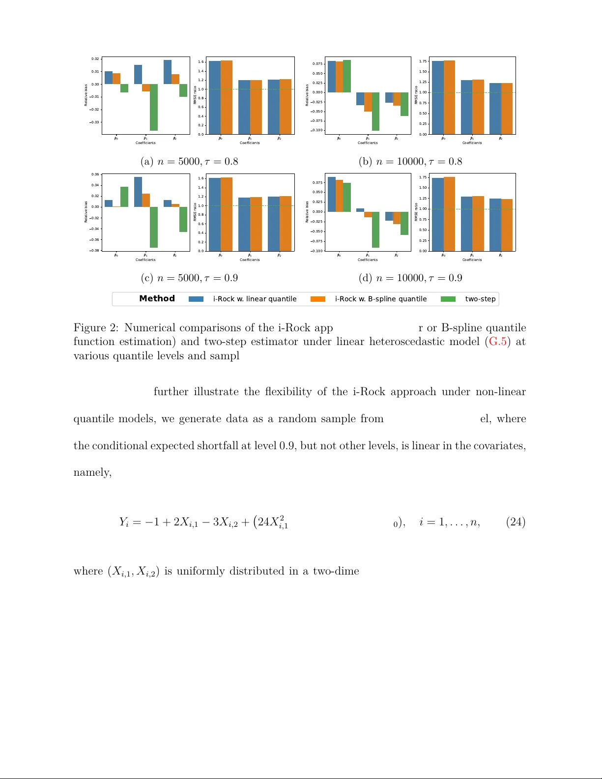
Exp ected Shortfall Regression via Optimization Y uanzhi Li † , Sh ush u Zhang † , Xuming He ‡ Univ ersit y of Mic higan † , W ashington Univ ersit y in St. Louis ‡ F ebruary 24, 2026 Abstract T o provide a comprehensiv e summary of the tail distribution, the exp ected short- fall is dened as the a verage ov er the tail ab o v e (or b elo w) a certain quantile of the distribution. The exp ected shortfall regression captures the heterogeneous cov ariate- resp onse relationship and describ es the cov ariate eects on the tail of the resp onse dis- tribution. Based on a critical observ ation that the superquantile regression from the op erations research literature do es not coincide with the exp ected shortfall regression, w e prop ose and v alidate a nov el optimization-based approac h for the linear exp ected shortfall regression, without additional assumptions on the conditional quan tile mo d- els. While the prop osed loss function is implicitly dened, we pro vide a protot ype implemen tation of the proposed approach with some initial exp ected shortfall esti- mators based on binning tec hniques. With practically feasible initial estimators, w e establish the consistency and the asymptotic normality of the proposed estimator. The prop osed approac h achiev es heterogeneit y-adaptiv e w eights and therefore often oers eciency gain o ver existing linear exp ected shortfall regression approaches in the literature, as demonstrated through simulation studies. K eywor ds: Conditional v alue-at-risk, sup erquan tile regression, data heterogeneit y , quan tile regression The rst two authors c ontribute d e qual ly to this work. 1 1 In tro duction The exp ected shortfall (ES), also known as the conditional v alue-at-risk (CV aR), measures the conditional mean of an outcome abov e (or below) a certain quantile. F ormally , the τ -th (upp er tail) ES of a random v ariable Y with E ( | Y | ) < ∞ is dened here as v [ Y ] ( τ ) = E [ Y | Y ≥ q [ Y ] ( τ )] , 0 ≤ τ < 1 , (1) where q [ Y ] ( τ ) is the τ -th quan tile of Y . W e consider the distribution of Y to b e con tinuous throughout the pap er. Then, v [ Y ] ( τ ) can b e equiv alen tly expressed as v [ Y ] ( τ ) = 1 1 − τ Z 1 τ q [ Y ] ( α ) d α . (2) The ES provides a useful summary of the tail distribution and has b ecome a p o w erful metric in a wide range of applications. In nance, the ES is a p opular risk measure as it is coheren t ( Artzner et al. 1999 , Acerbi & T asc he 2002 ) and quan ties the exp ected loss of a portfolio under adv erse scenarios ( Jorion 2003 , T opaloglou et al. 2002 , Kang et al. 2019 , Barendse et al. 2021 ). The ES has replaced the quan tile as the ocial risk metric for determining the regulatory minim um capital requiremen ts ( Basel Committee 2016 ). Bey ond nancial applications, the ES is useful in inv estigating heterogeneous treatmen t eects when the t wo p otential outcomes dier mainly in the tail ( He et al. 2010 , Zhang et al. 2025 , Chen & Y en 2024 ). As an example, we in v estigate the health disparities in lo w birth w eigh t among dieren t ethnic groups, where babies with low birth w eigh t tend to ha v e a higher risk of mortalit y and long-term health problems ( Hughes et al. 2017 ). The ES is also widely used in supply chain management ( Soleimani & Govindan 2014 , Sawik 2013 ), robust mac hine learning ( Laguel et al. 2021 a , b ), and reliabilit y engineering ( Ro ckafellar & 2 Ro yset 2010 ). In the presence of cov ariates, we are often interested in studying the relationship b etw een a set of cov ariates X and the tail of a resp onse v ariable Y . In this pap er, we mo del the conditional ES of Y giv en X in a linear framew ork. Sp ecically , w e assume that the cumulativ e distribution function of Y | X is contin uous. A t a xed quantile lev el τ ( 0 < τ < 1 ), we assume that v [ Y | X ] ( τ , x ) = E Y | Y ≥ q [ Y | X ] ( τ , x ) , X = x = x T β , (3) where q [ Y | X ] ( τ , x ) is the τ -th quantile of Y given X = x , and β is the τ -th ES regression co ecien t of interest. W e suppress the dependence on τ in β here for notational simplicit y . While the estimation and inference for the ES hav e b een well understo o d in the one- sample case ( Chen 2007 , Zwingmann & Holzmann 2016 , Sun & Cheng 2018 ), the literature on the linear ES regression mo del in ( 3 ) has gained more atten tion in recen t y ears. Due to the unelicitability of the ES ( Gneiting 2011 ), i.e., there do es not exist a loss function such that the ES is the minimizer of the exp ected loss, existing approaches for the linear ES regression often rely on quantile estimations or cumulativ e distribution function estimations that t ypically require additional mo deling assumptions b eyond ( 3 ). W e classify common linear ES regression metho ds into tw o categories and provide a brief review of each category . The rst category of approaches uses the equiv alen t denition of the ES in ( 2 ) and aggregates the conditional quantile or distribution functions in the tail. F or example, P eracc hi & T anase ( 2008 ) and Leorato et al. ( 2012 ) prop ose to use a weigh ted av erage of the quan tile regression estimators o ver a grid of quan tile lev els. More recently , Chetverik ov et al. ( 2022 ) prop oses to use an integration of non-parametric estimators of the conditional cum ulativ e distribution function, which do es not require parametric mo dels for the quantile 3 regression by lev eraging the technique of debiased machine learning ( Chernozhuk ov et al. 2018 ). The second category of approaches adopts a join t mo del for the τ -th quantile and the τ -th ES. Fissler & Ziegel ( 2016 ) recognizes that the quantile and ES are jointly elicitable as a pair. With this fact in mind, Dimitriadis & Bay er ( 2019 ) and P atton et al. ( 2019 ) dev elop a join t regression framew ork that estimates the quantile and ES regression simul- taneously . How ever, the asso ciated optimization problem is neither smo oth nor con vex, whic h p oses signicant computational challenges. Under the same joint regression mo dels for the quantile and the ES, tw o-step pro cedures hav e b een prop osed that estimate the τ -th quan tile and ES regression sequentially , whic h are computationally more con venien t ( Barendse 2020 , Peng 2022 , He et al. 2023 , Zhang et al. 2025 , Barendse 2023 ). A dditionally , non-parametric estimation of the ES regression is av ailable in the liter- ature. In addition to the w ork of Peracc hi & T anase ( 2008 ) and Leorato et al. ( 2012 ), Cai & W ang ( 2008 ) and Kato ( 2012 ) consider kernel-based approaches. Xiao ( 2014 ) uses the connection b et ween the ES and the chec k-loss function in the quan tile regression, and Martins-Filho et al. ( 2018 ) uses the extreme v alue theory . More recently , Olma ( 2021 ) con- siders lo cal-linear estimation based on Neyman-orthogonalized score functions. Nonethe- less, linear or parametric ES regression metho ds are often preferred for in terpretabilit y and statistical inference. In fact, w e will show later in the pap er that our proposed approac h w orks in the spirit of interpretable mac hine learning and aims to improv e statistical e- ciency and in terpretability by pro jecting a nonparametric ES function into a linear mo del. In this paper, we propose a nov el optimization form ulation for the linear ES regression mo del in ( 3 ) without additional mo deling assumptions on the quantile functions. This approac h is inspired by Ro c kafellar & Uryasev ( 2013 ) and Ro ckafellar & Royset ( 2014 ), 4 whic h estimate the ES by the sup erquantile dened as the minimizer of an implicitly dened loss function. While the sup erquan tile coincides with the ES in the one-sample case in ( 1 ), w e make it clear in Section 2 that the sup erquan tile regression is not the same as the ES regression in general. Our main contributions can b e summarized as follows. 1. W e prop ose and v alidate a new optimization framework for the ES regression that is motiv ated b y but distinctive from Ro ckafellar et al. ( 2014 ). W e show that the ES regression co ecient is the unique minimizer of a conv ex loss function that dep ends on some unknown distributional quantities. 2. Based on this new formulation, w e prop ose a practically feasible ES regression metho d, and show the consistency and asymptotic normality of the prop osed ES estimator. 3. Under appropriate conditions, w e show that the prop osed approac h is automatically adaptiv e to data heterogeneity , which explains its sup erior statistical eciency o ver existing ES regression approaches under a wide range of mo dels. The remainder of the pap er is organized as follo ws. W e provide a new characterization for the ES regression in Section 2 , whic h lays the foundation for our prop osed estimation metho d called i-Ro ck. Then w e describ e and explain how i-Ro ck w orks in problems with discrete co v ariates in Section 3 , where the op eration and the underlying statistical theory are cleaner and easier to understand. W e conduct further in v estigations of the i-Ro ck metho d for contin uous co v ariates in Section 4 , where some nonparametric initial estimates of the ES regression functions are used. The asymptotic analysis of the i-Ro ck estimator sho ws ho w it leans automatically tow ards go o d w eigh ting sc hemes in the presence of data heterogeneit y . W e demonstrate the practicality and numerical p erformance of the i-Ro c k metho d through numerical in vestigations in Section 5 and data applications on the health disparit y of low birth weigh t in Section 6 , follow ed b y some concluding remarks in Section 7 . 5 2 An optimization-based approac h for ES regression Let Y b e a random v ariable, with τ ∈ (0 , 1) as the quantile level of in terest, and X = (1 , ˜ X T ) T ∈ R p +1 as the cov ariate vector that includes an intercept term. In the one- sample case, Ro c kafellar & Uryasev ( 2013 ) and Ro c kafellar & Royset ( 2014 ) prop ose an optimization-based form ulation for the τ -th sup erquan tile of Y that coincides with the τ -th ES of Y in ( 2 ), i.e., v [ Y ] ( τ ) = argmin C C + 1 1 − τ Z 1 0 max { 0 , v [ Y ] ( α ) − C } d α. (4) Ho w ever, w e nd that a direct generalization to sup erquan tile regression do es not generally agree with the ES regression co ecients β in ( 3 ), ev en at the p opulation lev el, i.e., β 6 = argmin θ E ( X T θ ) + 1 1 − τ Z 1 0 max { 0 , v [ Y − X T θ ] ( α ) } d α ; (5) see App endix A for a review of the optimization formulation prop osed in Ro c kafellar & Ury asev ( 2013 ) and Ro ckafellar & Royset ( 2014 ), and a counterexample that prov es ( A.2 ). Giv en that sup erquan tile regression is not the solution to expected shortfall, w e dev elop a new optimization form ulation targeted for the ES regression under linear mo del ( 3 ). W e prop ose a p opulation-lev el loss function that can identify the τ -th conditional ES of Y giv en X , namely , L ( θ ) = E X Z 1 0 ρ τ v [ Y | X ] ( α, X ) − X T θ d α , (6) where ρ τ ( u ) = { τ − 1 ( u < 0) } u is the quan tile loss function ( K o enk er 2005 ), and E X denotes the exp ectation with resp ect to the random v ariable X . W e refer to L ( θ ) as 6 the improv ed Ro ckafellar (i-Ro ck) loss function, and refer to the pro cess of minimizing the i-Ro c k loss function as the i-Ro c k approach. In the case where | L ( θ ) | is innite, our analysis for the ES regression hereafter still holds b y considering the loss function E X h R 1 0 ρ τ v [ Y | X ] ( α, X ) − X T θ − ρ τ v [ Y | X ] ( α, X ) − X T β ∗ d α i for any given β ∗ , which is guaran teed to tak e nite v alues under the conditions of Theorem 2.1 b elow. The i-Ro c k loss function in ( B.1 ) is dieren t from the loss function in ( A.2 ), and we will show in Theorem 2.1 that the i-Ro c k approach yields the correct coecients for the ES regression. The extension from the one-sample ES loss function in ( A.1 ) to the new ES regression loss function in ( B.1 ) stands as a substantial impro v emen t that ensures the v alidity of the optimization-based approach for the ES regression. Theorem 2.1. Supp ose the cumulative distribution function of Y | X = x is c ontinuous and strictly incr e asing in a neighb orho o d of q Y | X ( τ , x ) , and the matrix D 1 = E X X X T v [ Y | X ] ( τ , X ) − q [ Y | X ] ( τ , X ) (7) is p ositive denite. Then, under line ar ES r e gr ession mo del ( 3 ) , β = argmin θ L ( θ ) , (8) wher e β is the true ES r e gr ession c o ecient and the minimizer is uniquely identie d. Theorem 2.1 shows that the ES regression co ecients are correctly and uniquely iden- tied by minimizing the i-Ro ck loss function under w eak conditions. A sucien t condition for D 1 to b e p ositiv e denite is that the components of X are linearly indep endent with probabilit y one. The i-Rock form ulation allows us to interpret the ES regression problem of Y on X as a quantile regression problem of Z on X , where Z is an auxiliary resp onse 7 v ariable distributed as Z | X ∼ v [ Y | X ] ( ξ , X ) where ξ ∼ U (0 , 1) and ξ is indep endent of X . This interpretation coincides with the fact that the τ -th quan tile of the ES pro cess at all levels from 0 to 1 is exactly the τ -th ES, due to the monotonicit y of v [ Y | X ] ( α, X ) ov er α ∈ (0 , 1) . This serves as an intuitiv e v alidation of the prop osed i-Ro c k formulation for the ES regression. Similar to the form ulation in ( A.1 ), the i-Ro c k form ulation in ( 8 ) is not directly feasible for empirical estimation since the i-Ro c k loss function ( B.1 ) inv olves unkno wn conditional ES pro cess at all quantile lev els from 0 to 1. In the remainder of the pap er, we formally prop ose and study a new estimation approac h for the ES regression based on the i-Ro c k form ulation, which, in essence, substitutes v [ Y | X ] ( α, X ) in ( B.1 ) with appropriate initial estimators. Typically , estimation of the ES w ould hav e high v ariabilit y at extreme quan tile lev els due to small eective sample sizes. As a corollary from Theorem 2.1 , we show that the i-Ro ck form ulation do es not necessarily inv olve the conditional ES at extreme tails. Corollary 1. F or any 0 < δ ≤ 1 , dene L ( δ ) ( θ ) = E X " Z τ + δ (1 − τ ) τ − δ τ ρ τ v [ Y | X ] ( α, X ) − X T θ d α # . Under the same c onditions of The or em 2.1 , we have β = argmin θ L ( δ ) ( θ ) , and the minimizer is uniquely identie d. T aking a small p ositive v alue δ , Corollary 1 sho ws that the domain of integration in the i-Ro c k loss function can b e muc h shortened without jeopardizing iden tication, v alidating a class of truncated i-Rock loss functions for the ES regression. Thus, only the conditional ES at quantile lev els near τ are relev ant for the i-Rock estimation of the τ -th ES regression. In the rest of the pap er, all deriv ations and exp ositions consider the case of δ = 1 , but 8 no essential changes are needed to cov er the case of δ ∈ (0 , 1) . In our numerical studies, w e use δ = 0 . 5 throughout the pap er. 3 The i-Ro c k approac h for discrete co v ariates T o demonstrate the i-Ro c k approach for ES regression, w e start with the simple setting with discrete cov ariates and study its theoretical prop erties. W e consider cov ariates that take only M distinct v alues, namely , { x 1 , . . . , x M } , where x m ∈ R p +1 , m = 1 , . . . , M , including an in tercept term, and M is a xed n umber that do es not dep end on the sample size. T o simplify notations, in this section, w e assume an equal num b er of i.i.d. observ ations at eac h co v ariate v alue with a total sample size of n , i.e., { ( x m , Y mj ) : m = 1 , . . . , M ; j = 1 . . . , n/ M } , (9) and w e write v [ Y | X ] ( s, x m ) as v m ( s ) and q [ Y | X ] ( s, x m ) as q m ( s ) . A simple initial ES estimator is the empirical ES at each distinct v alue of the cov ariates, namely , ˆ v m ( s ) = n/ M X j =1 Y mj 1 { Y mj ≥ ˆ q m ( s ) } (1 − s ) n/ M , m = 1 , . . . , M , (10) where ˆ q m ( s ) is the empirical s -th quan tile of the resp onses at x m . Under Mo del ( 3 ), the i-Ro c k estimator with discrete cov ariates is obtained through b β = argmin θ M X m =1 T X t =1 ρ τ ˆ v m ( α t ) − x T m θ , (11) 9 where α 1 , . . . , α T is an equally-spaced grid o ver the in terv al (0 , 1) for a suciently large T , with a pre-sp ecied δ ∈ (0 , 1) . Computationally , b β in ( 11 ) can b e obtained by the τ -th quantile regression of { ˆ v m ( α t ); t = 1 , . . . , T , m = 1 , . . . , M } on { x m ; t = 1 , . . . , T , m = 1 , . . . , M } , for which ecien t n umerical algorithms exist ( Koenker 2005 , Section 6). 3.1 Asymptotic results T o study the statistical prop erties of the i-Ro c k estimator in ( 11 ), w e start with sev eral tec hnical conditions on the data-generating mechanism. Condition R-X . The Gram matrix D 0 = P M m =1 x m x T m / M is p ositiv e denite. Condition R-Y1 . A t each x m , the cumulativ e distribution function of Y mj is con tinuous. F urthermore, the density function of Y mj , denoted as f m ( y ) , is b ounded a wa y from zero and contin uous on the interv al [ q m ( τ ) − ε, q m ( τ ) + ε ] for some ε > 0 . Condition R-Y2 . At eac h x m , E [( Y + mj ) 2 ] < + ∞ , where Y + mj = max { Y mj , 0 } . Condition R-X ensures the M distinct co v ariate v alues are non-degenerate. Conditions R-Y1 and R-Y2 are relatively weak for the resp onse distribution. Under Conditions R- Y1 and R-Y2 , v m ( α ) is increasing and con tin uously dieren tiable with resp ect to α for α ∈ [ τ − ϵ, τ + ϵ ] for some ϵ > 0 . With the inv erse empirical ES estimator denoted as ˆ h m ( z ) = inf { s ∈ [0 , 1] : ˆ v m ( s ) ≥ z } where ˆ v m ( s ) is the empirical ES estimator in ( 10 ), we presen t the main result for the i-Ro c k ES estimator in Theorem 3.1 . Theorem 3.1. Under a xe d discr ete design in ( 9 ) and Conditions R-X , R-Y1 , and R-Y2 , and supp ose D 1 = M − 1 P M m =1 { v m ( τ ) − q m ( τ ) } − 1 x m x T m is p ositive denite, we have (1 − τ ) D 1 b β − β = M − 1 M X m =1 x m h τ − ˆ h m { v m ( τ ) } i + o P 1 √ n . 10 In p articular, the i-R o ck estimator b β is c onsistent for β in ( 3 ) , and √ n b β − β d − → N 0 , D − 1 1 Ω 1 D − 1 1 , wher e Ω 1 = M − 1 P M m =1 σ 2 m ( τ ) { v m ( τ ) − q m ( τ ) } − 2 x m x T m , and (1 − τ ) σ 2 m ( τ ) = var [ Y m | Y m ≥ q m ( τ )] + τ [ v m ( τ ) − q m ( τ )] 2 . Theorem 3.1 uncov ers the main statistical prop erties of the i-Ro ck estimator, namely , consistency and asymptotic normality . It also gives an explicit connection b etw een b β and ˆ h m { v m ( τ ) } , the inv erse function of ˆ v m , via a Bahadur-type representation. While the implemen tation of the i-Ro c k approach only dep ends on ˆ v m as in ( 11 ), the rst-order asymptotic prop erty of b β depends directly and only on ˆ h m { v m ( τ ) } . Note that our consistency result in Theorem 3.1 is dierent from Theorem 3 in Ro c k- afellar et al. ( 2014 ) in the sense that the con v ergence limit for the Ro ck efellar’s estimator is not the ES regression co ecient, as demonstrated in Section 2 . This underscores the impro v ements ac hieved through our prop osed i-Ro c k approach for the ES regression. 3.2 Comparisons with other ES regression metho ds T o further understand the p erformance of the proposed i-Rock approach, w e compare its asymptotic eciency with the following four existing ES regression approac hes. Note that our prop osed i-Ro c k approach only assumes the linear ES regression mo del in ( 3 ), while all except for the linearization approac h b elo w assume linearity on b oth quan tile and ES, i.e., q [ Y | X ] ( τ ) = X T η , and ( 3 ). 1. The linearization approac h (LN) is to linearize the initial ES estimators, i.e., ˆ β = argmin u P M m =1 ( ˆ v m ( τ ) − x T m u ) 2 , where ˆ v m ( τ ) is dened in ( 10 ). 11 2. The joint approac hes (J1 and J2), prop osed in Fissler & Ziegel ( 2016 ), consider mo deling the quantile and the ES jointly by minimizing a joint loss function. Here, w e compare tw o dieren t sp ecications, J1 and J2, used by Dimitriadis & Bay er ( 2019 ) and Patton et al. ( 2019 ), resp ectively . 3. The tw o-step approach (TS), prop osed in Barendse ( 2020 ), is formulated as ˆ η = argmin η M X m =1 n/ M X j =1 ρ τ ( Y mj − x T m η ) , ˆ β = argmin β M X m =1 n/ M X j =1 Z mj ( ˆ η ) − x T m β 2 , where Z mj ( η ) = (1 − τ ) − 1 ( Y mj − x T m η ) 1 ( Y mj ≥ x T m η ) + x T m η . 4. The tw o-step least squares approach (TSLS) is formulated as ˆ η = argmin η M X m =1 n/ M X j =1 ρ τ ( Y mj − x T m η ) , b β = argmin θ M X m =1 n/ M X j =1 ( Y mj − x T m θ ) 2 · 1 { Y mj ≥ x T m ˆ η } . W e relegate the detailed formulations for these approac hes and their asymptotic v ariance to App endix C.2 of the Supplemen tary Material. W e shall examine the asymptotic eciencies of these metho ds in the following t wo examples. Case 3.1 W e consider the linear homoscedastic mo del, namely , Y mj = x T m η + ε mj , ( m = 1 , . . . , M ; j = 1 , . . . , n 0 ) , where P M m =1 x m x T m / M is p ositive denite, and ε mj ’s are i.i.d. with con tin uous density and nite second moment. Then, we hav e A V ar iRock = A V ar T S = A V ar LN = A V ar T S LS ≤ ( A V ar J 1 ∧ A V ar J 2 ) , where A V ar [ · ] denotes the asymptotic v ariance for eac h of the metho ds. Here, the i-Rock, the t w o-step, the linearization, and the t wo-step least squares estimators ac hiev e the same eciency . All of these approaches are at least as ecien t as the tw o join t approac hes, and they achiev e equal eciency if and only if x T m η are constan t o ver m . In fact, TS, J1, J2, and i-Ro ck estimators are asymptotically equiv alen t 12 0.7 0.9 1.1 1.3 i−Rock J1 J2 Method Frobenius norm ratio class i−Rock J1 J2 0.8 1.0 1.2 i−Rock J1 J2 Method determinant ratio class i−Rock J1 J2 Figure 1: The violin plot of ARE of the i-Ro ck and the join t approaches relativ e to the TS approac h, at τ = 0 . 9 under Mo del ( 13 ) with p = 3 . Here, the ARE of one estimator b β 1 relativ e to the other estimator b β 2 is dened as k A V ar ( b β 2 ) k / k A V ar ( b β 1 ) k , where k·k can b e F rob enius norm (on the left) and determinan t (on the right). Each element of the co v ariates ˜ X takes v alues indep endently from { i/ 10; i = 0 , 1 , . . . , 10 } with equal probabilit y . F or γ 1 = ( γ 10 , γ T 11 ) T and γ 2 = ( γ 20 , γ T 21 ) T , we x γ 10 = γ 20 = 3 and randomly sample 200 dieren t v alues of γ 11 and γ 21 indep enden tly and uniformly in the cub e [ − 1 , 3] 3 . to the weigh ted least squares estimator argmin u M X m =1 w m ˆ v m ( τ ) − x T m u 2 , (12) with w eights w m prop ortional to 1 , { v m ( τ ) } − 2 , { v m ( τ ) } − 3 / 2 , and { v m ( τ ) − q m ( τ ) } − 1 , re- sp ectiv ely . In this case, the joint approaches lose eciency b y incorp orating non-constan t w eigh ts in homoscedastic mo dels, while the i-Ro c k approach is ecient since the weigh t v m ( τ ) − q m ( τ ) remains constant o v er m in homoscedastic mo dels. Case 3.2 Next, we consider the heteroscedastic lo cation-scale shift mo del, namely , Y m = x T m γ 1 + ( x T m γ 2 ) · ε mj ( m = 1 , . . . , M ; j = 1 , . . . , n 0 ) , (13) 13 where x T m γ 2 > 0 , ε mj ’s are i.i.d. and follow a (scaled) normal distribution with v [ ε mj ] ( τ ) = 0 and v ar { ε mj | ε mj > q [ ε mj ] ( τ ) } = 1 . Under this more complicated mo del, w e present empir- ical results of the asymptotic relativ e eciency (ARE) under 200 randomly sampled mo del parameter v alues in Figure 1 . The i-Rock approach is more ecient than the TS approach in almost all cases, ev en though the latter requires an additional mo deling assumption on the quantile function. The key to this improv ement is the implicit w eighting induced b y the i-Ro c k loss function, as will b e discussed in Section 4.1 . Under Mo del ( 13 ), the i-Ro ck approac h is asymptotically equiv alent to ( 12 ) with w m ∝ ( x T m γ 2 ) − 1 . While w m are not optimal, they are b enecial for eciency since w m reects the disp ersion of Y m on the righ t tail and do wn-weigh ts data with higher conditional tail v ariance. On the other hand, the p erformance of the joint approaches v aries heavily with γ 1 and γ 2 in ( 13 ), resulting in up to a 20% increase or decrease in eciency compared to the TS approach. In summary , none of the approac hes considered here are universally the most ecient since none can achiev e optimal asymptotic weigh ts. How ev er, the i-Rock approach is more ecien t in most cases since its asymptotic weigh t w m ∝ { v m ( τ ) − q m ( τ ) } − 1 c haracterizes the data heterogeneity and often aligns closer to the optimal weigh ts. 4 The i-Ro c k approac h for con tin uous co v ariates T o pro vide general guidance and further theoretical inv estigations of the prop osed i-Ro c k approac h, we no w consider the i-Ro c k approac h with con tinuous co v ariates, applicable also to a mix of con tinuous and discrete co v ariates. While the same principles giv en in Section 3 apply , the theoretical analysis in this section is muc h more inv olved. The key c hallenge arises from using initial estimators for the conditional ES under minimal assumptions. W e start with a general analysis for a broad class of non-parametric initial ES estimators and 14 sho w that the i-Ro ck approach is asymptotically equiv alen t to a weigh ted linearization of those initial estimators. T o b e specic, we also consider an example of the initial estimator, namely , the Neyman-orthogonalized lo cally linear ES estimator. The pro of of the three theorems in this section can b e found in App endix D of the Supplementary Material. W e form ulate our i-Rock approac h for contin uous cov ariates with the idea of binning to simplify the subsequent theoretical analysis. Supp ose { ( X i , Y i ) : i = 1 , . . . , n } is a random sample from the distribution ( X, Y ) ∼ Pr. In the remainder of the paper, w e shall write the conditional ES and quantile of Y | X = x as v ( τ , x ) and q ( τ , x ) , resp ectiv ely , omitting the subscript [ Y | X ] . Let X ⊂ R p +1 b e the sample space of the co v ariate, and we partition X = S M m =1 A m , where A 1 , . . . , A M are non-sto c hastic, disjoint bins, and the n umber of bins M may grow with sample size n . Within eac h bin A m , let ¯ x m ∈ R p +1 b e the geometric cen ter of A m , i.e., ¯ x m = | A m | − 1 R x 1 { x ∈ A m } d x with | A m | b eing the v olume of the bin, and let ˆ v ( α, ¯ x m ) b e an initial estimator of v ( α, ¯ x m ) , for α ∈ (0 , 1) . Under Mo del ( 3 ), the i-Ro c k estimator is formulated as b β = argmin u ∈ R p +1 M X m =1 ˆ γ m Z 1 0 ρ τ ˆ v ( α, ¯ x m ) − ¯ x T m u d α, (14) where ˆ γ m is a user-sp ecied w eight for eac h bin A m . While w e allo w man y c hoices of ˆ γ m , w e w ould normally set ˆ γ m to b e the bin size of A m , to adjust for the dierences in sample sizes across bins. In practice, we may approximate the integration in ( 14 ) by a ne grid ov er α ∈ (0 , 1) , whic h turns ( 14 ) into a quantile regression problem in terms of computation. 4.1 Asymptotic linearization of the i-Ro c k estimator Let f Y | X ( y ; x ) b e the conditional density function of Y | X = x . W e further imp ose the follo wing regularity conditions. 15 Condition G-X . The co v ariates hav e b ounded supp ort X ⊂ R p +1 , and ha v e a densit y function f X ( x ) that is uniformly b ounded aw ay from 0 and + ∞ on X . F urthermore, the matrix D 1 dened in ( 7 ) is p ositive denite. Condition G-Y1 . A t each x , f Y | X ( y ; x ) is con tin uous o ver y . There exist constants f , f , and ε 0 > 0 , such that 0 < f ≤ inf ( x,y ): x ∈X | y − q ( τ ,x ) |≤ ε 0 f Y | X ( y ; x ) ≤ sup ( x,y ): x ∈X | y − q ( τ ,x ) |≤ ε 0 f Y | X ( y ; x ) ≤ f . Condition G-Y2 . F or eac h x , q ( s, x ) and v ( s, x ) are strictly increasing and contin uous o ver s ∈ (0 , 1) . F urthermore, q ( τ , x ) and v ( τ , x ) are Lipsc hitz contin uous as a function of x . Condition G-V1 . F or an y m = 1 , . . . , M , the initial ES estimator ˆ v ( s, ¯ x m ) is left-con tin uous and non-decreasing in s ∈ (0 , 1) . F urthermore, for any constan t B > 0 and some sequence r n = o ( n − 1 / 4 ) , the initial estimator satises (i) sup m =1 ,...,M s : | s − τ |≤ B · ( r n + n − 1 / 2 ) | ˆ v ( s, ¯ x m ) − v ( s, ¯ x m ) | = O P ( r n ) , (ii) sup m =1 ,...,M s : | s − τ |≤ B · ( r n + n − 1 / 2 ) | [ ˆ v ( s, ¯ x m ) − v ( s, ¯ x m )] − [ ˆ v ( τ , ¯ x m ) − v ( τ , ¯ x m )] | = o P n − 1 / 2 . Condition G-V2 . The weigh ted aggregation of the initial ES estimators satises M X m =1 ˆ γ m ¯ x m v ( τ , ¯ x m ) − q ( τ , ¯ x m ) { ˆ v ( τ , ¯ x m ) − v ( τ , ¯ x m ) } = O P n − 1 / 2 . Conditions G-X , G-Y1 and G-Y2 are standard in the literature of quantile and ES regression; see, e.g., ( Koenker 2005 , Section 4), and Dimitriadis & Bay er ( 2019 ). The b ounded supp ort assumption in Condition G-X is mathematically necessary if we allow data heterogeneit y and are in terested in l inear ES functions at tw o dieren t quantile levels. In practical problems, we usually w ork with cov ariates with b ounded ranges. Conditions G- V2 and G-V1 imp ose generally weak assumptions on the initial ES estimators that allo w 16 for a broad class of non-parametric ES estimations. Condition G-V1 requires uniform consistency with a con v ergence rate slightly b etter than n 1 / 4 and asymptotic equicon tin uit y of the estimated ES pro cess. Condition G-V2 requires that a weigh ted aggregation of the initial ES estimators ov er bins enjoys a n 1 / 2 -rate of con v ergence. As discussed in Corollary 1 , our analysis w ould only concern ˆ v ( s, x ) for those s in a local neigh b orho od of τ , but not at extreme quantile levels, as long as ˆ v ( s, x ) is monotonic in s . W e relegate further discussion of the initial ES estimator to App endix F of the Supplementary Material. Recall from ( 14 ) that ˆ γ m is a weigh t for each bin in the i-Ro c k approach, and that the n um b er of bins M may dep end on the sample size. Let diam ( · ) b e the diameter of a set in R p +1 , and let ˆ π m = n − 1 P n i =1 1 [ X i ∈ A m ] b e the prop ortion of data that fall in to the bin A m . In the following theorem, we establish the asymptotic relationship b etw een the prop osed i-Ro ck estimator and its initial ES estimators. Theorem 4.1. Supp ose Conditions G-X , G-Y1 and G-Y2 hold. In addition, supp ose that the binning me chanism and the chosen weights satisfy sup m =1 ,...,M diam ( A m ) = o (1) and sup m =1 ,...,M ˆ γ m ˆ π m − 1 = o P (1) . Given any initial ES estimator that satises Conditions G-V1 and G-V2 , the i-R o ck estimator in ( 14 ) satises b β − β = D − 1 1 M X m =1 ˆ γ m ¯ x m v ( τ , ¯ x m ) − q ( τ , ¯ x m ) { ˆ v ( τ , ¯ x m ) − v ( τ , ¯ x m ) } + o P ( n − 1 / 2 ) , wher e D 1 is dene d in ( 7 ) . In p articular, b β is √ n -c onsistent for β . Theorem 4.1 implies that b β is asymptotically equiv alen t to a w eigh ted linearization of ˆ v ( τ , ¯ x m ) ov er each bin. The i-Rock approach turns a set of non-parametric initial estimators in to a parametric estimator via the i-Ro c k loss function in ( 14 ). Sp ecically , consider the 17 follo wing weigh ted least squares (WLS) of the initial τ -th ES estimator on the cov ariates e β = min u ∈ R p +1 M X m =1 ˆ γ m w m ˆ v ( τ , ¯ x m ) − ¯ x T m u 2 , (15) where w m is a set of known w eights. With simple linear algebra, e β satises e β − β = M X m =1 ˆ γ m w m ¯ x m ¯ x T m ! − 1 M X m =1 [ ˆ γ m w m ¯ x m { ˆ v ( τ , ¯ x m ) − v ( τ , ¯ x m ) } ] . (16) Com bining ( 16 ) and Theorem 4.1 , we note that the i-Ro c k estimator b β in ( 14 ) is asymp- totically equiv alent to e β in ( 15 ) with w m = [ v ( τ , ¯ x m ) − q ( τ , ¯ x m )] − 1 . One key feature of the i-Ro c k approach is that the weigh ts are implicit and automatic. Direct calculation of the WLS w ould require estimating the unknown weigh ts w m . Plugging in estimated w eights ˆ w m ma y lead to unstable WLS estimates where there is not a sucient amoun t of data. Another feature of the i-Ro ck approac h is that the w eigh ts are adaptiv e to heterogeneit y in a go o d wa y . Among the class of WLS estimators in ( 15 ), the optimal w eigh t w ∗ m ∝ { v ar [ ˆ v ( τ , ¯ x m )] } − 1 reects the heterogeneity of the initial estimators (see, e.g., Section 7 of W o oldridge ( 2010 )). Although the eective weigh ts for the i-Ro ck approach may not b e optimal, they tend to b e w ell correlated with w ∗ m . Olma ( 2021 ) shows that non-parametric conditional ES estimators often hav e asymptotic v ariance in the form of a n v ar [ ˆ v ( τ , ¯ x m ) | X = ¯ x m ] = ρ 1 v ar [ Y | X = ¯ x m , Y ≥ q ( τ , ¯ x m )] + ρ 2 [ v ( τ , ¯ x m ) − q ( τ , ¯ x m )] 2 + o P (1) , (17) where a n is a scaling factor, and ρ 1 , ρ 2 are tw o constan ts dep ending on the construction of ˆ v ( τ , x ) . The weigh t w m = [ v ( τ , ¯ x m ) − q ( τ , ¯ x m )] − 1 captures part of the v ariance in ( 17 ), and in many cases, the tw o additive components in ( 17 ) are often well correlated across 18 x m b ecause they b oth capture the spread of the conditional distribution on the right tail. Therefore, the i-Ro ck approach can often be more ecient than a simple linearization approac h that do es not adapt well to the heterogeneity in the data. 4.2 Asymptotic normality In this section, w e provide a concrete example of the initial ES estimator that satises the tec hnical conditions of Theorem 4.1 , and establish the asymptotic normality of the i-Ro c k estimator with suc h an initial ES estimator. In particular, we t a bin-wise linear ES regression with a Neyman-orthogonalized score function in Barendse ( 2020 ), namely , (ˆ c 0 , ˆ c 1 ) = argmin c 0 ∈ R c 1 ∈ R p X X i ∈ A m h ˆ Z i ( s ) − c 0 − c T 1 ( ˜ X i − ˜ x m ) i 2 , ˆ v ( s, ¯ x m ) = ˆ c 0 , (18) where ˆ Z i ( s ) = (1 − s ) − 1 { Y i − ˆ q ( s, X i ) } 1 { Y i ≥ ˆ q ( s, X i ) } + ˆ q ( s, X i ) , X i = (1 , ˜ X T i ) T , and ¯ x m = (1 , ˜ x T m ) T . With this initial ES estimator, w e obtain the i-Ro c k estimator in ( 14 ) with ˆ γ m = S 0 m − S T 1 m S − 1 2 m S 1 m , n − 1 X T m W m X m = S 0 m S T 1 m S 1 m S 2 m . (19) This ES estimation approach is similar to that in Olma ( 2021 ) with a k ey dierence that w e do not require any sp ecic form of the quantile estimator ˆ q ( s, x ) , as long as it satises Condition G-Q in App endix D.1 of the Supplementary Material. F or mo dels with linear quan tile functions, this condition is readily satised. Theorem 4.2. Under Conditions G-X , G-Y2 , and G-Y1’, G-A1, G-A2, G-Q in A pp endix D.1, the initial ES estimator c onstructe d in ( D.1 ) satises Conditions G-V1 and G-V2 , thus the c onclusion of The or em 4.1 holds. In p articular, the i-R o ck estimator ( 14 ) with 19 initial estimator in ( D.1 ) and ˆ γ m in ( D.2 ) satises √ n b β − β d − → N(0 , D − 1 1 Ω 1 D − 1 1 ) , (20) wher e Ω 1 = E σ 2 τ ( X )[ v ( τ , X ) − q ( τ , X )] − 2 X X T , and (1 − τ ) σ 2 τ ( x ) = var ( Y | X = x, Y ≥ q ( τ , x )) + τ [ v ( τ , x ) − q ( τ , x )] 2 . Theorem 4.2 shows that our lo cally linear ES estimator in ( D.1 ) satises Conditions G-V1 and G-V2 required by Theorem 4.1 , and therefore can b e used as an initial estimator for the i-Ro c k approac h. F urthermore, the resulting asymptotic v ariance-cov ariance matrix in Theorem 4.2 has the same form as that in Theorem 3.1 for discrete cov ariates. Compared to the case with discrete cov ariates, the main technical c hallenges b ehind Theorem 4.2 can b e summarized as follows. First, the num b er of bins M = M n increases with the sample size. Therefore, the uniform con vergence rate of the initial estimators o v er the bins needs to b e carefully in v estigated. Second, we need to establish the pro cess con v ergence of ˆ v ( s, ¯ x m ) for a con tin uum of s . Standard empirical pro cess to ols do not apply directly to the binned data. Moreov er, we also need to explicitly analyze the bias in ˆ v ( s, ¯ x m ) attributed to binning and quantile estimation. 4.3 Optimal weigh ting and eciency comparison T o achiev e optimal w eigh ts under the weigh ted least-squares framework in ( 16 ), w e tak e it further with additional weigh ts ω m on the i-Ro ck loss function, namely , b β = argmin u ∈ R p +1 M X m =1 ˆ γ m ω m Z 1 0 ρ τ ˆ v ( α, ¯ x m ) − ¯ x T m u d α. (21) 20 W e sho w that ω m = v ( τ , x m ) − q ( τ , x m ) σ 2 τ ( x m ) , (22) where σ 2 τ ( · ) is dened in Theorem 4.2 , is the theoretically optimal weigh ts in this class. Theorem 4.3. Under the same assumptions of The or em 4.2 , the weighte d i-R o ck estimator ( 21 ) – ( 22 ) achieves the minimum asymptotic varianc e attainable under the weighte d le ast- squar es fr amework ( 15 ) , with the asymptotic varianc e h E n X X T σ 2 τ ( X ) oi − 1 . W e also note that the optimally w eighted i-Ro c k estimator is asymptotically equiv alent to the optimal join t M-estimator in Dimitriadis et al. ( 2022 ) as w ell as the optimally w eigh ted tw o-step approach in Barendse ( 2020 ). W e defer the detailed comparison of the three optimally weigh ted approaches to App endix D.7.1. In practice, the optimal weigh ts of all these approaches need to b e estimated from data. An interesting feature of the (un w eighted) i-Ro ck approach is that it corresp onds to implicit weigh ts in the framework of ( 15 ) that adapt well to data heterogeneit y automatically and are usually highly correlated with the optimal weigh ts as discussed at the end of Section 4.1 . On the other hand, for general mo del classes, the optimally w eigh ted ES regression estimators giv en here may still ha v e an eciency gap with the semiparametric eciency giv en in Dimitriadis et al. ( 2022 ). The comparisons ab ov e assume that w e ha ve linear (or parametric) quan tile function sp ecications, which is not needed for the the i-Ro ck approac h. In other words, the i-Ro c k estimators tend to b e more robust against deviations from linear quantile mo dels. In our empirical w ork, w e nd that the (unw eighted) i-Ro ck estimators can b e compara- ble to the optimally weigh ted tw o-step estimators when the weigh ts are estimated from the data; see App endix D.7.2. In those cases, the estimation of the w eigh ts leads to some loss of nite-sample eciency , further arguing for the v alue of the automatic i-Ro c k approach without weigh t estimation for data of mo derate sizes. 21 5 Numerical in v estigations In this section, we demonstrate the practical applicabilit y of the i-Rock estimator and in v estigate its numerical p erformance through simulation studies. F or discrete cov ariates, w e implemen t the i-Ro ck approach in Algorithm 1 from App endix G.1 of the Supplementary Material based on Section 3 and Corollary 1 . F or contin uous or mixed co v ariates, we adopt a v ariant of ( 14 ) summarized in Algorithm 2 of the Supplemen tary Material, which uses the bin-wise lo cal-linear initial ES estimator introduced in Section D.1 . In particular, we partition the cov ariate space b y binning each cov ariate. Discrete cov ariates are naturally partitioned according to their distinct v alues, while con tinuous co v ariates are divided using breakp oin ts at equally spaced quan tiles. F or subsequen t exp erimen ts, we set the n um b er of bins for eac h contin uous cov ariate as k = d 1 . 6 √ p × { √ n/ log ( n ) } 1 /p e , where p refers to the num b er of contin uous cov ariates with a slight abuse of notation. W e rep ort simulation studies to compare the p erformance of the i-Ro ck approac h with that of the t w o-step approach discussed in Section 3.2 , and to chec k the approximate nor- malit y of the i-Ro ck estimator in nite-samples. W e defer the comparison with the “quan tile a v erage metho d,” whic h inv olves a v eraging ov er a series of linear quan tile estimators from quan tile levels τ to 1 , to App endix G.3 of the Supplementary Material. In our studies with con tinuous cov ariates, w e consider t wo types of quan tile function estimators in ( D.1 ), namely , the (global) linear quan tile and the B-spline quan tile estimators. The linear quan- tile estimation uses all the av ailable data to t a linear quantile regression. The B-spline quan tile estimation uses additiv e piecewise linear quan tile function where t wo in ternal knots are placed at the 1 / 3 and 2 / 3 quantiles of each observed cov ariate. W e compare our pro- p osed i-Ro c k implementation with the t wo-step estimator prop osed by Barendse ( 2020 ) in terms of the relative bias and the Root Mean Squared Error (RMSE). More specically , w e 22 use 500 replications to calculate (1) the relativ e bias ( ¯ β i − β i ) /S D ( ˆ β ( j ) i ) , where β i is the i -th comp onen t of β , ˆ β ( j ) i is the estimator for β i in the j -th replicate, and ¯ β i = 1 500 P 500 j =1 ˆ β ( j ) i ; and (2) the Ro ot Mean Squared Error (RMSE) ratio of the tw o-step approach o v er the i-Ro c k approach, with a ratio greater than 1 indicating b etter eciency for the i-Rock estimator. F or the remainder of this section, w e denote X i,j as the j -th comp onen t of X i , and consider b ounded cov ariates as in our theory . W e add that the prop osed estimator still p erforms w ell if w e are only in terested in one quan tile level and the linear model holds o v er an un b ounded cov ariate, or correlated co v ariates, as demonstrated in App endix G.4 of the Supplementary Material. Case 5.1 W e generate data as a random sample from a linear heteroscedastic mo del with t w o-dimensional cov ariates, namely , Y i = { 1 + U } + (2 + 2 U ) X i, 1 + { 3 + 3 U } X i, 2 , i = 1 , . . . , n, (23) where U follo ws U (0 , 1) , X i, 1 follo ws U (0 , 4) , and X i, 2 are indep endently distributed from { 0 , 1 } with equal probability . Figure 15 shows the relative bias and the RMSE ratio com- parisons for τ ∈ { 0 . 8 , 0 . 9 } and n ∈ { 5000 , 10000 } . The i-Ro ck estimators with b oth the linear and the B-spline quantile regression estimation outp erform the tw o-step estimator in bias and RMSE in all settings. This is consistent with the theoretical nding in Sec- tion 3.2 that the i-Ro ck approach oers a b etter adaptation to heterogeneity . At these relativ ely large sample sizes, w e verify that the sampling distribution of the i-Ro ck esti- mator ( ˆ β 0 , ˆ β 1 , ˆ β 2 ) follows a normal distribution with the theoretical asymptotic v ariances in ( 20 ) v ery closely by Kolmogoro v–Smirnov test; see Appendix G.2 of the Supplemen tary Material. 23 0 1 2 Coefficients 0.03 0.02 0.01 0.00 0.01 0.02 R elative bias 0 1 2 Coefficients 0.0 0.2 0.4 0.6 0.8 1.0 1.2 1.4 1.6 RMSE ratio (a) n = 5000 , τ = 0 . 8 0 1 2 Coefficients 0.100 0.075 0.050 0.025 0.000 0.025 0.050 0.075 R elative bias 0 1 2 Coefficients 0.00 0.25 0.50 0.75 1.00 1.25 1.50 1.75 RMSE ratio (b) n = 10000 , τ = 0 . 8 0 1 2 Coefficients 0.08 0.06 0.04 0.02 0.00 0.02 0.04 0.06 R elative bias 0 1 2 Coefficients 0.0 0.2 0.4 0.6 0.8 1.0 1.2 1.4 1.6 RMSE ratio (c) n = 5000 , τ = 0 . 9 0 1 2 Coefficients 0.100 0.075 0.050 0.025 0.000 0.025 0.050 0.075 R elative bias 0 1 2 Coefficients 0.00 0.25 0.50 0.75 1.00 1.25 1.50 1.75 RMSE ratio (d) n = 10000 , τ = 0 . 9 Method i-R ock w . linear quantile i-R ock w . B-spline quantile two -step Figure 2: Numerical comparisons of the i-Ro ck approach (with linear or B-spline quantile function estimation) and tw o-step estimator under linear heteroscedastic mo del ( G.5 ) at v arious quantile lev els and sample sizes. Case 5.2 T o further illustrate the exibility of the i-Ro ck approach under non-linear quan tile mo dels, w e generate data as a random sample from the following mo del, where the conditional exp ected shortfall at level 0.9, but not other levels, is linear in the cov ariates, namely , Y i = − 1 + 2 X i, 1 − 3 X i, 2 + 24 X 2 i, 1 + 12 X 2 i, 2 + 5 ( ϵ i − ν 0 ) , i = 1 , . . . , n, (24) where ( X i, 1 , X i, 2 ) is uniformly distributed in a tw o-dimensional square [ − 1 , 2] 2 , ϵ i follo ws the sk ewed- t 5 distribution with skewness 2 ( Theo dossiou 1998 ) that is indep endent of the co v ariates, and ν 0 is the 0 . 9 -th ES of the distribution of ϵ i . Figure 12 shows the results for τ = 0 . 9 , n = 10000 . In this case, b oth the i-Ro ck with linear quantile function estimation and the tw o-step estimator suer from the missp ecication of the quan tile function, while the i-Ro c k with the B-spline quantile function estimation is signicantly less biased and 24 0 1 2 Coefficients 0 2 4 6 8 10 R elative bias Method i-R ock w . linear quantile i-R ock w . B-spline quantile two -step 0 1 2 Coefficients 0 1 2 3 4 RMSE ratio Method i-R ock w . linear quantile i-R ock w . B-spline quantile two -step Figure 3: Numerical comparisons of the i-Ro ck approach (with linear or B-spline quantile function estimation) and tw o-step approach under Mo del ( G.2 ) at τ = 0 . 9 , n = 10000 . more ecien t than the tw o-step estimator (with the RMSE ratios as high as 5.2). The asymptotic normality for the i-Ro ck estimators with B-spline quan tile function is numeri- cally conrmed with the Q-Q plots in Figure 4 of the Supplementary Material. Case 5.3 T o further ev aluate the sup erior adaptation to data heterogeneit y of the i-Rock approac h, we generate data from a t w o-dimensional mo del where the heterogeneity of the conditional distribution is more evident than in the earlier cases, namely , Y i = { 1 − log(1 − U ) } + (2 + 2 U ) X i, 1 + { 3 − 30 log(1 − U ) } X i, 2 , i = 1 , . . . , n, (25) where U is uniformly distributed on (0 , 1) , and ( X i, 1 , X i, 2 ) are indep endently distributed from binomial (2 , 0 . 5) . The RMSE ratios are summarized in T able 1 at sev eral sample sizes. In this case, the i-Ro c k estimator is signican tly more ecien t than the t wo-step estimator, due to the automatic eective w eighting sc hemes of the former. n β 0 β 1 β 2 1000 7.19 7.18 1.61 2000 9.23 7.69 1.50 5000 10.41 8.64 1.63 T able 1: RMSE ratio of the tw o-step estimator ov er the i-Ro ck estimator under mo del ( G.3 ). 25 6 Data Application Lo w birth weigh t is long-known to b e asso ciated with increased infant mortalit y risk and long-term health issues; See Hughes et al. ( 2017 ) for a recent review. The health disparity for infants with lo w birth w eigh ts among dieren t ethnic groups has drawn increasing atten tion from policy mak ers, suc h as the National Institutes of Health (NIH) and the Cen ters for Disease Control and Preven tion (CDC) ( Osterman et al. 2024 ), among other researc hers ( Burris & Hac ker 2017 , Su et al. 2021 , Pollock et al. 2021 ). In this example, w e use ES regression to inv estigate the p ossible con tributing factors of racial disparities for lo w birth weigh t. W e naturally fo cus on the lo w er (left-tail) ES of the birth weigh t distribution conditional on other factors, and measure the racial disparity as the dierences in terms of the lo wer ES at a giv en quan tile lev el (e.g., τ = 0 . 05 ) b etw een t wo ethnic groups. Let Y denote the birth weigh t, and R = 1 and 0 represent one of the disadv antaged group (e.g., Blac k, Asian, or Hispanic) and the ma jorit y group (White in this example), resp ectively , with X as other factors under consideration. F or each disadv antaged group, we dene the health disparit y function at a given cov ariate X = x and a pre-sp ecied quan tile lev el τ as d ( τ , x ) = v [ − Y | ( R,X )] { 1 − τ , (1 , x ) } − v [ − Y | ( R,X )] { 1 − τ , (0 , x ) } , (26) where the upper tail ES of − Y is used here to replicate the lo w er tail of Y and be consisten t with our theory in this pap er. W e use the 2022 U.S. birth-w eigh t dataset, whic h is av ailable online at the National Cen- ter for Health Statistics ( https://www.cdc.gov/nchs/data_access/vitalstatsonline. htm ). In this example, w e fo cus on male singleton births only , and include the follo w- ing p oten tial risk factors: mother’s race, age, education level, presence of gestational di- 26 T able 2: Estimated co ecien ts for the lo wer ES regression of birth w eight at the quan tile lev el τ = 0 . 05 using the i-Ro c k approach. The num b ers in the parenthesis show the standard errors. Co v ariates Co ecien ts Co v ariates Co ecien ts (In tercept) 1627.34 ( 5.37 ) Gestational diab etes (baseline: no gestational diab etes) -34.02 ( 6.20 ) Race = blac k (baseline: white) -249.97 ( 7.98 ) Gestational h yp ertension (baseline: no gestational hypertension) -447.88 ( 4.57 ) Race = asian (baseline: white) -193.55 ( 6.27 ) Cigarettes at 3rd trimester (baseline: no cigarette use at 3rd trimester) -174.59 ( 5.68 ) Race = hispanic (baseline: white) -61.77 ( 1.12 ) Mother’s age < 20 (baseline: age [20 , 34] ) -19.98 ( 14.25 ) Prenatal visits ∈ [6 , 10] (baseline: [0 , 5] ) 437.05 ( 6.24 ) Mother’s age > 34 (baseline: age [20 , 34] ) -94.45 ( 4.31 ) Prenatal visits > 10 (baseline: [0 , 5] ) 832.55 ( 5.85 ) Receipt of WIC (baseline: not receipt of WIC) 8.25 ( 3.11 ) Education: ≥ college (baseline: high school and b elow) 63.21 ( 4.36 ) Unmarried (baseline: married) -77.56 ( 5.99 ) Education: some college (baseline: high school and b elow) -4.25 ( 4.72 ) ab etes or h yp ertension, smoking during the third trimester, n um b er of prenatal visits, receipt of a Sp ecial Supplemental Nutrition Program for W omen, Infants, and Children (WIC), and parents’ marital status. In particular, the WIC is a program designed to help lo w-income pregnan t women, infants, and children up to age 5 receive prop er n utrition b y pro viding v ouchers for fo o d, nutrition counseling, health care screenings and referrals ( https://www.fns.usda.gov/wic/about- wic- glance ). After combining b oth the U.S. data and U.S. T erritories Data, and remo ving entries with missing v alues for the v ariables of interest, we ha v e a total of n = 1 , 534 , 031 observ ations, including 826 , 367 as White, 226 , 327 as Blac k, 774 , 24 as Asian, and 359 , 118 as Hispanic individuals. Due to the p o- ten tial non-linear relationship b et ween birth w eigh t and mother’s age and the num b er of prenatal visits, w e discretize age (in y ears) in to three categories: < 20 , [20 , 34] (as baseline) and > 34 ; and w e discretize the num b er of prenatal visits into three categories: ≤ 5 (as baseline), [6 , 10] , and > 10 . T o estimate the health disparity function ( 26 ) at τ = 0 . 05 , w e start with a linear mo del 27 6-10 >10 Number of pr enatal visits 200 150 100 50 0 50 1 0 Black Asian Hispanic Figure 4: The quantities shown from part of β 1 − β 0 asso ciated with Equation ( 27 ) are the birth w eigh t disparities (the lo w er 0 . 05 ES) of the disadv an taged groups for subgroups dened b y the num b er of prenatal visits: [6 , 10] and > 10 , with the subgroup of ≤ 5 prenatal visits serving as the baseline. for the low er ES of the birth w eight against the dumm y v ariables for all four races and the other p oten tial risk factors. The regression co ecien ts and their standard errors calculated b y the bo otstrap are summarized in T able 6 . With the additiv e mo del, the health disparit y in ( 26 ) for eac h race is constan t across the other factors X and equals the corresp onding ES regression coecient. F or example, the results sho w that the a verage low est 5% of the birth w eigh t of the Blac k p opulation is lo wer (than that of the White p opulation) by around 250 grams. The dierence is around 193 grams for Asians and 45 grams for Hispanics. Since the additiv e linear mo del across all races is quite ten tativ e, we no w t the linear ES regression separately for eac h race, which amounts to allowing tw o-wa y interactions b et w een race and other factors X . Under this mo del, the health disparity function ( 26 ) can b e written as d ( τ , x ) = x T ( β 1 − β 0 ) , (27) where β 1 and β 0 represen t the ES regression co ecien t at level τ for a disadv an taged racial group and the ma jority group (i.e., White), respectively . Conditioning on all the other factors, the prenatal visits and gestational hypertension are tw o notew orth y factors to the health disparit y across all disadv antaged races, according to the estimates for β 1 − 28 T able 3: The p ercen tages of participants receiving WIC and unmarried, resp ectiv ely , for dieren t ethnic groups, stratied b y the n umber of prenatal visits. The num b ers in paren- thesis show the p ercentages of individuals in the categories of prenatal visits within eac h race group. Race White Blac k Hispanic # of prenatal visits [0 , 5] [6 , 10] > 10 [0 , 5] [6 , 10] > 10 [0 , 5] [6 , 10] > 10 (5.96%) (31.19%) (62.85%) (13.78%) (38.74%) (47.48%) (11.87%) (39.63%) (48.50%) Receipt of WIC(%) 24.9 20.4 17.5 40.2 45.8 45.5 44.71 46.79 45.86 Unmarried(%) 44.5 28.9 24.9 77.7 70.0 66.6 64.52 54.81 49.92 β 0 presen ted in Figure 13 in App endix G.5 of the online Supplemen tary Materials. In particular, Figure 4 shows the estimated components of β 1 − β 0 corresp onding to prenatal visits, representing the dierences in the disparit y b et ween each disadv antaged racial groups and White individuals when the n umber of prenatal visits is in [6 , 10] or > 10 , as compared to the subgroup of no more than 5 prenatal visits. It is in teresting to note that the disparities of Blac k and Hispanic relativ e to White are most eviden t when the n umber of prenatal visits is high ( > 10 times). T o elucidate p ossible explanations for this phenomenon, we perform a logistic regression for the binary indicator for prenatal visits ( > 10 times versus ≤ 5 times) on the other co v ariates separately for eac h race and compare the co ecients across races. W e nd that ho w WIC enrollment and marital status asso ciate with the frequency of prenatal visits diers across racial groups. In T able 3 , we present the p ercentages of WIC receipt and unmarried women, stratied b y race and n um b er of prenatal visits. The results sho w that the p ercentage of the receipts of the WIC de cr e ases as the n um b er of prenatal visits increases for White w omen, whereas the p ercentage actually increases among Blac k and Hispanic women. Despite p otentially b eneting from the WIC program interv entions, Black and Hispanic women with more frequen t prenatal visits ma y hav e lo w er so cio economic status and w ealth compared to their White counterparts. This so cio economic gap may exacerbate disparities for the subgroup with more than 10 prenatal visits. Marital status may also pla y a role, as the unmarried 29 p ercen tage decreases drastically with more prenatal visits for White w omen, but not as eviden t for Black and Hispanic w omen. In this application, combining ES regression with mean and quantile regression provides additional insights, as detailed in App endix G.5. 7 Conclusions and discussions In this pap er, we prop ose a new optimization-based approach to the ES regression estima- tion. In contrast to the sup erquantile regression estimator of Ro ckafellar et al. ( 2014 ), the prop osed estimator is consistent for the ES regression co ecient under heterogeneit y . Relativ e to other metho ds of ES regression estimation, the i-Ro ck approach has inter- esting and desirable prop erties and has unique challenges of its own. Compared with the computationally simpler tw o-step approach ( Barendse 2020 ), the i-Ro ck estimator has sev- eral adv an tages: it automatically incorporates heterogeneit y-adaptiv e w eights and do es not require a linear assumption in the quan tile mo del. If optimal weigh ts are estimated from the data and then used in these metho ds, b oth estimators achiev e the same asymptotic eciency . The joint estimation of quan tile and ES regressions oers additional bandwidth for the construction of estimators, and data-adaptiv ely c hosen loss functions can lead to the same asymptotic eciency as the optimally weigh ted i-Ro c k metho d. How ev er, such join t estimation metho ds ha ve to nd solutions that optimize non-con v ex and non-smo oth loss functions, while the i-Ro ck estimator uses con v ex optimization. The ma jor c hallenge in the i-Ro ck approac h is the need to rely on initial ES regression estimates at a grid of quantile levels near the target quantile level τ . This increases the computational burden as well as the theoretical complexity in analyzing the resulting ES regression estimators. On the other hand, if we op erate under the framework with linear quan tile functions, as is assumed for the tw o-step or the joint estimation metho ds, the 30 computational and the theoretical complexities of the i-Ro ck estimators are greatly reduced. In tuitiv ely , the prop osed i-Ro ck approach enhances the in terpretabilit y of non-linear mac hine learning mo dels by pro jecting a nonparametric mo del to a linear function in the spirit of interpretable mac hine learning. W e hope that the i-Ro ck approach prop osed in the pap er op ens a new window of opp ortunities for the exp ected shortfall regression mo deling and interpretable machine learning asso ciated with exp ected shortfall analysis b oth in theory and in practice. 8 A c kno wledgmen t The researc h was supp orted in part by the National Science F oundation A w ards DMS- 2345035 and DMS-1951980. The authors rep ort there are no comp eting interests to declare. They also extend their gratitude to the anon ymous Asso ciate Editor and referees for their constructiv e comments, whic h contributed to impro vemen ts in the pap er. 31 Supplemen t to “Exp ected Shortfall Regression via Optimization” In this supplemen t, we pro vide the pro ofs, additional n umerical results and discussions, and the co de to the man uscript “Exp ected Shortfall Regression via Optimization” . W e con tinue to use the notations and n umbered equations from the main manuscript. Con ten ts 1 In tro duction 2 2 An optimization-based approac h for ES regression 6 3 The i-Ro c k approac h for discrete cov ariates 9 3.1 Asymptotic results . . . . . . . . . . . . . . . . . . . . . . . . . . . . . . . 10 3.2 Comparisons with other ES regression metho ds . . . . . . . . . . . . . . . 11 4 The i-Ro c k approac h for con tin uous co v ariates 14 4.1 Asymptotic linearization of the i-Ro ck estimator . . . . . . . . . . . . . . . 15 4.2 Asymptotic normalit y . . . . . . . . . . . . . . . . . . . . . . . . . . . . . 19 4.3 Optimal w eighting and eciency comparison . . . . . . . . . . . . . . . . . 20 5 Numerical in vestigations 22 6 Data Application 26 7 Conclusions and discussions 30 32 8 A c kno wledgmen t 31 A Ro c kafellar’s sup erquantile regression 36 A.1 The Ro c kafellar formulation revisited . . . . . . . . . . . . . . . . . . . . . 36 A.2 A counterexample on the regression formulation . . . . . . . . . . . . . . . 37 B Pro of of theoretical results in Section 2 40 B.1 Pro of of Theorem 2.1 . . . . . . . . . . . . . . . . . . . . . . . . . . . . . . 41 B.2 Pro of of Corollary 1 . . . . . . . . . . . . . . . . . . . . . . . . . . . . . . 44 C Pro of and additional details of Section 3 44 C.1 Pro of of Theorem 3.1 . . . . . . . . . . . . . . . . . . . . . . . . . . . . . . 44 C.1.1 Auxiliary results for the one-sample ES pro cess . . . . . . . . . . . 44 C.1.2 Pro of for the one-sample case . . . . . . . . . . . . . . . . . . . . . 48 C.1.3 Pro of for the i-Ro c k approach with discrete cov ariates . . . . . . . 54 C.2 Other ES regression approac hes in Section 3.2 . . . . . . . . . . . . . . . . 62 C.2.1 Description of the approac hes . . . . . . . . . . . . . . . . . . . . . 63 C.2.2 Asymptotic v ariance for the comp eting approaches . . . . . . . . . 65 C.2.3 Additional empirical results . . . . . . . . . . . . . . . . . . . . . . 67 D Pro of and additional details of Section 4 67 D.1 An initial ES estimator . . . . . . . . . . . . . . . . . . . . . . . . . . . . . 67 D.2 Some technical lemmas . . . . . . . . . . . . . . . . . . . . . . . . . . . . . 72 D.3 Pro of of Theorem 4.1 . . . . . . . . . . . . . . . . . . . . . . . . . . . . . . 76 D.4 Pro of of Theorem 4.2 . . . . . . . . . . . . . . . . . . . . . . . . . . . . . . 82 D.5 Pro of of Prop ositions 2, 3 and 4 . . . . . . . . . . . . . . . . . . . . . . . . 84 D.5.1 Pro of of Prop osition 2 . . . . . . . . . . . . . . . . . . . . . . . . . 84 33 D.5.2 Pro of of Prop osition 3 . . . . . . . . . . . . . . . . . . . . . . . . . 92 D.5.3 Pro of of Prop osition 4 . . . . . . . . . . . . . . . . . . . . . . . . . 100 D.6 Pro of of Theorem 4.3 . . . . . . . . . . . . . . . . . . . . . . . . . . . . . . 109 D.7 W eighted ES regression approaches . . . . . . . . . . . . . . . . . . . . . . 111 D.7.1 Eciency comparison . . . . . . . . . . . . . . . . . . . . . . . . . 111 D.7.2 Empirical results . . . . . . . . . . . . . . . . . . . . . . . . . . . . 114 E Pro of of tec hnical lemmas 117 E.1 Pro of of Lemma C.3 . . . . . . . . . . . . . . . . . . . . . . . . . . . . . . 117 E.2 Pro of of Lemma C.4 . . . . . . . . . . . . . . . . . . . . . . . . . . . . . . 118 E.3 Pro of of Lemma D.1 . . . . . . . . . . . . . . . . . . . . . . . . . . . . . . 120 E.4 Pro of of Lemma D.2 . . . . . . . . . . . . . . . . . . . . . . . . . . . . . . 121 E.5 Pro of of Lemma D.3 . . . . . . . . . . . . . . . . . . . . . . . . . . . . . . 122 E.6 Pro of of Lemma D.4 . . . . . . . . . . . . . . . . . . . . . . . . . . . . . . 127 E.7 Pro of of Lemma D.5 . . . . . . . . . . . . . . . . . . . . . . . . . . . . . . 132 F Discussions on initial ES estimator for the i-Ro c k approach 135 F.1 On the non-linearity of the initial ES estimator . . . . . . . . . . . . . . . 135 F.2 On the monotonicity of the initial ES estimator . . . . . . . . . . . . . . . 136 F.3 On the bias in the initial ES estimator . . . . . . . . . . . . . . . . . . . . 137 G Numerical inv estigations 138 G.1 Implemen tation . . . . . . . . . . . . . . . . . . . . . . . . . . . . . . . . . 138 G.2 Asymptotic normality c heck for Section 5 . . . . . . . . . . . . . . . . . . . 139 G.3 Comparisons to quan tile av erage approac h . . . . . . . . . . . . . . . . . . 141 G.4 A dditional simulation results . . . . . . . . . . . . . . . . . . . . . . . . . . 145 34 G.5 A dditional results to Section 6 . . . . . . . . . . . . . . . . . . . . . . . . . 146 35 A Ro c kafellar’s sup erquan tile regression In this section, w e start with a brief review of the optimization formulation for the su- p erquan tile estimation prop osed in Ro ckafellar & Ury asev ( 2013 ) and Ro c kafellar & Ro y- set ( 2014 ). In con trast to the one-sample case, we demonstrate through a counterexample that the ES regression coecient in ( 3 ) is not a solution to the sup erquantile regression in Ro c kafellar et al. ( 2014 ). A.1 The Ro c kafellar form ulation revisited Let Y b e a random v ariable and τ ∈ (0 , 1) b e the quan tile level of interest. The τ -th sup erquan tile of Y , denoted as ˜ v [ Y ] ( τ ) , is dened exactly the same as the τ -th ES of Y in ( 2 ). By Theorem 1 of Ro ckafellar et al. ( 2014 ), the τ -th sup erquan tile of Y is the minimizer of a loss function with unknown p opulation quantities ˜ v [ Y ] ( α ) for α ∈ (0 , 1) , i.e., ˜ v [ Y ] ( τ ) = argmin C C + 1 1 − τ Z 1 0 max { 0 , ˜ v [ Y ] ( α ) − C } d α (A.1) Giv en a nite sample, one can substitute the function ˜ v [ Y ] ( α ) in ( A.1 ) by an empirical es- timator to obtain a feasible conv ex optimization formulation for the sup erquantile. Ro ck- afellar & Ro yset ( 2018 ) prop oses ecien t numerical algorithms for ( A.1 ) via a dual metho d that do es not require an explicit estimation of ˜ v [ Y ] ( α ) in adv ance. Since ˜ v [ Y ] ( τ ) = v [ Y ] ( τ ) in the one-sample case, this optimization-based formulation provides a conceptually v aluable alternativ e to the ES estimation. 36 A.2 A counterexample on the regression form ulation Let X = (1 , ˜ X T ) T ∈ R p +1 b e the cov ariate v ector that includes an intercept term. By Section 3.1 of Ro ckafellar et al. ( 2014 ), the sup erquantile regression co ecient is dened as the minimizer of a function directly extended from ( A.1 ), namely , ˜ β = argmin θ E ( X T θ ) + 1 1 − τ Z 1 0 max { 0 , ˜ v [ Y − X T θ ] ( α ) } d α . (A.2) Ho w ever, with a simple coun terexample, w e illustrate that the sup erquantile regression co ecien t ˜ β in ( A.2 ) do es not coincide with the ES regression co ecien ts β from ( 3 ), even at the p opulation level. Consider the follo wing mo del with p = 1 Y = 1 + ˜ X ε, (A.3) where ˜ X ∼ Γ(2 , 1) with E ( ˜ X ) = 2 , and ε ∼ U ( − 1 , 1) that is indep enden t of ˜ X . W e aim to estimate the 0 . 5 ES regression, where the true ES regression co ecien ts are β 0 = 1 , β 1 = 0 . 5 . T o nd the minimizer to the p opulation level loss function in ( A.2 ) at τ = 0 . 5 , we note from Prop osition 3 of Ro ckafellar et al. ( 2014 ) that solving ( A.2 ) is equiv alen t to the follo wing tw o-step pro cedure: θ ∗ 1 ← arg min θ 1 E ( ˜ X T θ 1 ) + 1 1 − τ Z 1 τ v [ Y − ˜ X T θ 1 ] ( α ) d α | {z } L 1 ( θ 1 ) , (A.4) θ ∗ 0 ← v [ Y − ˜ X T θ ∗ 1 ] ( τ ) , (A.5) where θ ∗ 0 and θ ∗ 1 are the p opulation-level minimizers, and the co v ariates are X T = (1 , ˜ X T ) . W e compute the analytical expression for the marginal sup erquantile of Z ( θ 1 ) = Y − 37 ˜ X T θ 1 for an y θ 1 and an y quan tile level. F or any θ 1 ∈ ( − 1 , 1) , Z ( θ 1 ) follo ws tilted double exp onen tial distribution with density function, f Z ( θ 1 ) ( z ; θ 1 ) = 1 2 exp n z 1+ θ 1 o , z < 0 , 1 2 exp n − z 1 − θ 1 o , z ≥ 0 . Straigh tforw ard probabilistic calculation sho ws that the marginal sup erquan tile of Z ( θ 1 ) = Y − θ 1 ˜ X is v [ Z ( θ 1 )] ( α ) = 1 + 1 1 − α α (1 + θ 1 )(1 − log h 2 α 1+ θ 1 i ) − 2 θ 1 , 0 ≤ α ≤ 1+ θ 1 2 , 1 + ( θ 1 − 1) log h 2(1 − α ) 1 − θ 1 i − 1 , 1+ θ 1 2 < α < 1 . (A.6) Substituting Equation ( A.6 ) into the loss function in ( A.2 ), w e can obtain an analytical expression for the loss function L 1 ( θ 1 ) . Moreo ver, w e can compute the rst-order deriv ative to the loss function L 1 ( θ 1 ) as: ∂ L 1 ( θ 1 ) ∂ θ 1 = E ( ˜ X ) + 1 1 − 1 / 2 Z 1 1 / 2 ∂ v [ Y − ˜ X T θ 1 ] ( α ) ∂ θ 1 dα = − 1 − log(1 − θ 1 ) , − 1 ≤ θ 1 ≤ 0 , 2 − 1 2 − Li 2 ( 1 2 ) + Li 2 ( θ 1 +1 2 ) + ( 1 2 − log 2) log (1 + θ 1 ) , 0 < θ 1 ≤ 1 , where Li 2 ( x ) = − R x 0 log(1 − z ) /z dz . Figure 5 b elow shows the loss function in ( A.2 ) and its deriv ativ e under Mo del ( A.3 ). 38 Since the loss function in ( A.2 ) is con vex and dierentiable ( Rockafellar et al. 2008 , Ro ck- afellar & Ury asev 2013 ), w e can use a rst-order metho d, e.g., the Newton-Raphson metho d, to solv e the minimization problem ( A.2 ). W e use the con v ex optimization toolb ox in MA T- LAB and obtain the p opulation-lev el minimizer to ( A.2 ) as ˜ β 1 = 0 . 7041 , mark ed b y the red line in Figure 5 , while the true ES regression coecient is β 1 = 0 . 5 , mark ed b y the blue line. Note we fo cus on the population lev el loss function, therefore the clear discrepancy b et w een ˜ β 1 and β 1 sho ws the superquantile regression approach prop osed b y Ro c kafellar et al. ( 2014 ) fails to give the correct co ecients for the ES regression. 1 -1 -0.5 0 0.5 1 θ 2.5 3 3.5 4 4.5 5 L( θ ) -1 -0.5 0 0.5 1 θ -2 -1.5 -1 -0.5 0 0.5 1 ∂ L/ ∂ θ Figure 5: The p opulation lev el loss function L 1 ( θ 1 ) (left panel) and its deriv ative (righ t panel). The blue dashed line marks the true ES regression co ecien t β 1 , while the red one marks the minimizer of L 1 ( θ 1 ) . W e further demonstrate the inconsistency of the sup erquantile regression approach b y Ro c kafellar et al. ( 2014 ) using a n umerical exp erimen t. W e generate 200 Mon te Carlo datasets from Mo del ( A.3 ), and w e consider sample sizes at n = 100 or n = 1000 . Setting τ = 0 . 5 , Figure 6 sho ws the histogram of the estimated slope term ˆ β 1 among the 200 Monte Carlo datasets, solv ed b y the n umerical in tegration metho d in Section 5.2 of Ro c kafellar et al. ( 2014 ) with 100 grid p oints. W e can see the histograms are clearly concen trating to w ard ˜ β 1 = 0 . 704 , instead of the true ES regression co ecien t β 1 = 0 . 5 . While the sup erquantile regression prop osed in Ro ckafellar et al. ( 2014 ) is not v alid for the ES regression, it can still b e v aluable as a generalized regression technique. As 1 Although the foregoing deriv ation for L 1 ( θ 1 ) is only v alid for θ ∈ (0 , 1) , it do es not aect our conclusion. This is due to the global conv exity of the loss function in ( A.2 ) ( Ro ckafellar et al. 2008 ): A lo cal minimizer within [ − 1 , 1] m ust also b e the global minimizer. 39 C 1 Frequency 0.2 0.4 0.6 0.8 0 5 10 15 20 25 C 1 Frequency 0.50 0.55 0.60 0.65 0.70 0.75 0.80 0 5 10 15 20 25 30 Figure 6: The empirical distribution of the estimator ˆ β 1 follo wing Rockafellar et al. ( 2014 ) at sample size n = 100 (left) and n = 1000 (right). The blue line marks the true ES regres- sion co ecien t β 1 = 0 . 5 , while the red one marks the p opulation-lev el solution to ( A.2 ), namely , ˜ β 1 = 0 . 704 . sho wn in Ro ckafellar & Uryasev ( 2013 ), the sup erquantile regression approac h nds the b est linear appro ximation to the resp onse Y using the cov ariates X , in the sense that the residuals minimize the sup erquantile loss function ( A.2 ). F urthermore, Ro ckafellar & Ro yset ( 2018 ) shows that the sup erquantile regression co ecient in ( A.2 ) is consistent for the ES regression in homoscedastic linear mo dels; and Golo dnik o v et al. ( 2019 ) shows that the sup erquan tile regression approac h is equiv alen t to a composite quan tile regression under certain scenarios. Therefore, the sup erquantile regression approach can b e useful for risk tuning and optimization that incorp orates cov ariate information ( Miranda 2014 ). B Pro of of theoretical results in Section 2 Recall that w e omit the subscript [ Y | X ] of v and ˆ v , q , and ˆ q , and simply write as v ( s, x ) , ˆ v ( s, x ) , q ( s, x ) , ˆ q ( s, x ) , resp ectiv ely , throughout the pro of. 40 B.1 Pro of of Theorem 2.1 Pr o of. In order to show that the true ES co ecient β is the unique minimizer of the loss function L ( θ ) = E X Z 1 0 ρ τ v [ Y | X ] ( α, X ) − X T θ d α , (B.1) where ρ τ ( u ) = { τ − 1 ( u < 0) } u is the quantile loss function, we break the pro of into the follo wing three steps: (1) w e show that the function v ( u, x ) is increasing in u ∈ (0 , 1) and strictly increasing in u ∈ [ τ − ϵ, τ + ϵ ] for each p ossible v alue of x ; (2) we verify the rst- order optimality condition; (3) w e chec k the p ositiv e deniteness of the Hessian matrix at the minim um. F rom the prop erty of the quan tile loss function, (see, e.g., K o enk er ( 2005 , Chapter 1.3)), the loss function in ( B.1 ) is con v ex in θ . Combined with (2) and (3), it follo ws that β is the unique global minimizer of the loss function. Step 1 F or eac h x , w e chec k the monotonicit y of v ( u, x ) ov er u . The conditional quantile of Y | X = x , i.e., q ( u, x ) , is increasing in u ∈ (0 , 1) b y denition. Then, by denition of v ( u, x ) , i.e., v ( u, x ) = (1 − u ) − 1 Z 1 u q ( s, x )d s, (B.2) w e ha v e that v ( u, x ) is increasing in u ∈ (0 , 1) since it is a tail-av erage of q ( u, x ) . Since the cumulativ e distribution function of Y | X = x is con tin uous and strictly increasing in a neighborho o d of q ( τ , x ) , q ( u, x ) is contin uous and strictly increasing in u ∈ [ τ − ϵ, τ + ϵ ] for some ϵ > 0 . F or u ∈ [ τ − ϵ, τ + ϵ ] and for all x , v ( u, x ) = (1 − u ) − 1 ( (1 − τ ) v ( τ , x ) + Z τ u q ( s, x ) d s ) 41 is nite since v ( τ , x ) is nite for all x and q ( s, x ) are b ounded on a closed interv al due to con tin uity . Therefore, for u ∈ [ τ − ϵ, τ + ϵ ] , ∂ v ( u, x ) ∂ u = ∂ { (1 − u ) − 1 R 1 u q ( s, x )d s } ∂ u = R 1 u q ( s, x )d s (1 − u ) 2 − q ( u, x ) 1 − u = v ( u, x ) − q ( u, x ) 1 − u (B.3) = 1 (1 − u ) 2 Z 1 u [ q ( s, x ) − q ( u, x )] d s > 0 . Hence v ( u, x ) is strictly increasing in u ∈ [ τ − ϵ, τ + ϵ ] . Step 2 Next, w e c heck the rst-order optimalit y condition of β for the loss function L ( θ ) in ( B.1 ). By dening ξ ∼ U (0 , 1) , w e equiv alently write L ( θ ) as L ( θ ) = E ( X, ξ ) ρ τ v ( ξ , X ) − X T θ . (B.4) F rom the prop ert y of the chec k-loss function ρ , it follows that the function L ( θ ) is conv ex and dierentiable in θ . Then, ∂ L ( θ ) ∂ θ θ = β = E ( X,ξ ) τ − 1 v ( ξ , X ) < X T β · ( − X ) = E X τ − Pr ξ | X v ( ξ , X ) < X T β | X · ( − X ) = E X τ − Pr ξ | X { v ( ξ , X ) < v ( τ , X ) | X } · ( − X ) = E X ([ τ − Pr ( ξ < τ )] · ( − X )) = 0 , 42 where the second equality follows b y rst conditioning on X , the third equalit y follo ws from v ( τ , X ) = X T β , the fourth equalit y follows from the monotonicit y of v ( u, x ) in step 1, and the last equalit y follo ws from ξ ∼ U (0 , 1) and indep endent of X . The rst-order optimality condition, combined with the conv exity of L ( θ ) , implies that β is the global minimum. Step 3 Lastly , we show the minimizer of L ( θ ) is unique. Since L ( θ ) is conv ex, it suces to show that the Hessian matrix at the minimum is p ositiv e denite. Since v ( · , x ) is strictly monotone, let h ( z , x ) b e the inv erse of v ( · , x ) , suc h that v ◦ ( h ( z , x ) , x ) = z . By the conditions in Theorem 2.1, we ha ve ∂ Pr ( v ( ξ , x ) ≤ z ) ∂ z z = v ( τ ,x ) = ∂ Pr ( ξ ≤ h ( z , x )) ∂ z z = v ( τ ,x ) = ∂ h ( z , x ) ∂ z z = v ( τ ,x ) = ∂ s ∂ v ( s, x ) s = τ = ( ∂ v ( s, x ) ∂ s s = τ ) − 1 = 1 − τ v ( τ , x ) − q ( τ , x ) . (B.5) Therefore, L ( θ ) is twice dieren tiable, and its second deriv ative at θ = β satises ∂ 2 L ∂ θ ∂ θ T θ = β = E X ∂ Pr ξ | X ( v ( ξ , X ) ≤ z ) ∂ z z = X T β · X X T = E X ∂ Pr ξ ( v ( ξ , x ) ≤ z ) ∂ z ( z = X T β ,x = X ) · X X T = (1 − τ ) E X X X T v ( τ , X ) − q ( τ , X ) = (1 − τ ) D 1 0 , 43 where the second equality follo ws since ξ is indep enden t of X , and the third equalit y follo ws from ( B.5 ) and v ( τ ) = x T β . Therefore, the Hessian matrix of L ( · ) ev aluated at β is positive denite, establishing the uniqueness of the minimizer β . B.2 Pro of of Corollary 1 Pr o of. It follo ws closely from the pro of to Theorem 2.1 in App endix B.1 by simply replacing the distribution of ξ to ξ ∼ U ( τ − δ τ , τ + δ (1 − τ )) and noting that Pr ( ξ < τ ) = τ . C Pro of and additional details of Section 3 C.1 Pro of of Theorem 3.1 In order to show the consistency and the asymptotic normality of the i-Ro ck estimator with discrete cov ariates in Theorem 3.1, we start with one-sample case without cov ariates in C.1.1 and C.1.2 , and generalize to the case with discrete cov ariates in C.1.3 . C.1.1 Auxiliary results for the one-sample ES pro cess W e rst presen t asymptotic results in the one-sample case without an y co v ariate. These results also apply to the empirical ES estimators at each co v ariate v alue in our regression setting. W e x some notations for the discussion of the one-sample problem. Suppose the data Y 1 , . . . , Y n are i.i.d. observ ations with a common distribution function F ( y ) . F or an y 0 < s < 1 , let ˆ q ( s ) b e the sample quan tile from the n observ ations, we dene the empirical 44 ES estimator as: ˆ v ( s ) = P n i =1 Y i · 1 { Y i ≥ ˆ q ( s ) } P n i =1 1 { Y i ≥ ˆ q ( s ) } . (C.1) While the parameter of in terest is the τ -level ES, here we consider the empirical ES pro cess, whic h is the sto chastic pro cess giv en b y { ˆ v ( s ) : s ∈ [ τ L , τ U ] } , where 0 < τ L < τ < τ U < 1 . Let ℓ ∞ [ a, b ] b e the set of all uniformly b ounded functions on the interv al [ a, b ] . T o further simplify notations, in the remainder of this subsection, w e shall write ˆ v s = ˆ v ( s ) and ˆ q s = ˆ q ( s ) , and w e dene q L and q U as the τ L -th and τ U -th quan tile, resp ectively . In the one-sample case, the notations here may be dierent than those in the regression setting. W e need the follo wing tec hnical condition, which is the one-sample coun terpart for Conditions R-Y1 and R-Y2. Condition U . The distribution function F ( y ) is con tinuously dieren tiable on the in terv al [ q L − ε, q U + ε ] for some ε > 0 ; the density function f ( y ) is b ounded a wa y from zero and ab o v e on the same in terv al. F urthermore, we ha ve E [ Y 2 · 1 { Y ≥ 0 } ] < + ∞ . No w we present the rst main result in the one-sample case, whic h concerns the weak con v ergence of the empirical ES as a sto c hastic pro cess indexed b y the quantile lev el. Not only is the result an important technical to ol for subsequen t analysis, but it also is of in terest on its own. Theorem C.1. Supp ose Condition U holds, then we have ˆ v s − v s = 1 n n X i =1 ( Y i − q s ) · 1 ( Y i ≥ q s ) 1 − s − ( v s − q s ) + o P n − 1 / 2 , uniformly in s ∈ [ τ L , τ U ] . F urthermor e, the c enter e d empiric al ES pr o c ess c onver ges we akly: √ n [ ˆ v ( · ) − v ( · )] ⇝ G ( · ) in ℓ ∞ [ τ L , τ U ] , 45 wher e G ( · ) is a me an zer o Gaussian Pr o c ess. Theorem C.1 giv es the uniform (weak) Bahadur representation for the empirical ES pro cess. T o the b est of our kno wledge, the uniformit y of the result is new. Restricting to a single quantile lev el τ , Chen ( 2007 ) and Zwingmann & Holzmann ( 2016 ) study the asymptotic prop erties of the ES estimator ˆ v ( τ ) under more general conditions; on the other hand w e discuss pro cess conv ergence. Practically , Theorem C.1 is a tec hnical to ol for sim ultaneous statistical inference for a range of exp ected shortfalls. As a simple corollary of Theorem C.1 , we can obtain the asymptotic distribution for the τ -level empirical ES, which is also kno wn from, e.g., Chen ( 2007 ) and Zwingmann & Holzmann ( 2016 ). Corollary 2. Under Condition U , we have √ n ( ˆ v τ − v τ ) d − → N(0 , σ 2 τ ) , with (1 − τ ) σ 2 τ = var ( Y | Y ≥ q τ ) + τ ( v τ − q τ ) 2 . Pr o of. Combining the Central Limit Theorem with the Bahadur represen tation in Theorem 46 C.1 concludes the results with asymptotic v ariance σ 2 τ = v ar ( Y − q τ ) · 1 ( Y ≥ q τ ) 1 − τ − ( v τ − q τ ) = E ( Y − q τ ) 2 · 1 ( Y ≥ q τ ) (1 − τ ) 2 + ( v τ − q τ ) 2 − 2( v τ − q τ )( Y − q τ ) · 1 ( Y ≥ q τ ) 1 − τ = E { ( Y − v τ ) 2 + ( v τ − q τ ) 2 + 2( Y − v τ )( v τ − q τ ) | Y ≥ q τ } P ( Y ≥ q τ ) (1 − τ ) 2 + ( v τ − q τ ) 2 − 2( v τ − q τ ) E ( Y − q τ | Y ≥ q τ ) P ( Y ≥ q τ ) 1 − τ = E { ( Y − v τ ) 2 | Y ≥ q τ } + ( v τ − q τ ) 2 1 − τ − ( v τ − q τ ) 2 = 1 1 − τ { v ar ( Y | Y ≥ q τ ) + τ ( v τ − q τ ) 2 } The asymptotic v ariance σ 2 τ consists of t wo parts. The rst part is the v ariance in esti- mating v τ when q τ is kno wn, whereas the second part is attributable to quan tile estimation ( Zwingmann & Holzmann 2016 ). Next, we proceed to the study of the inv erse ES function, whic h we dene b elow: h ( z ) = { s : v s = z } and ˆ h ( z ) = inf { s ∈ [0 , 1] : ˆ v s ≥ z } , for any z ∈ [ v τ L , v τ U ] . Note v s is strictly increasing in s ∈ [ τ L , τ U ] , and w e sho w in Lemma C.3 that ˆ v ( z ) is also non-decreasing in s ∈ [ τ L , τ U ] ; therefore the denitions ab o ve are w ell-dened. The follo wing Lemma shows that ˆ h ( z ) , the empirical inv erse ES, is also asymptotically Gaussian. Lemma C.2. Under Condition U , the inverse ES pr o c ess satises: ˆ h ( z ) − h ( z ) = − 1 n n X i =1 ( Y i − q h ( z ) ) · 1 { Y i ≥ q h ( z ) } z − q h ( z ) − (1 − h ( z )) + o P n − 1 / 2 , 47 uniformly in z ∈ [ v τ − ε ′ , v τ + ε ′ ] for some ε ′ > 0 . In p articular, we have: √ n ˆ h ( v τ ) − τ d − → N 0 , (1 − τ ) 2 σ 2 τ ( v τ − q τ ) 2 , with σ 2 τ dene d in Cor ol lary 2 . F urthermor e, the pr o c ess n 1 / 2 [ ˆ h ( z ) − h ( z )] is asymptotic al ly e qui-c ontinuous over z ∈ [ v τ − ε ′ , v τ + ε ′ ] with r esp e ct to the Euclide an distanc e. The asymptotic prop ert y of ˆ h ( z ) is essen tial for the analysis of the i-Ro c k regression approac h. The pro of of Lemma C.2 builds up on the uniform represen tation in Theorem C.1 , as well as the functional Delta metho d; See, e.g., Theorem 20.8 in V an der V aart ( 2000 ). Note, the asymptotic normality of ˆ v τ at a single level ( Chen 2007 , Zwingmann & Holzmann 2016 ), is not sucient to establish the result in Lemma C.2 . C.1.2 Pro of for the one-sample case The pro ofs in this subsection rely on standard empirical pro cess to ols in, e.g., V an Der V aart & W ellner ( 1996 ), and we adopt the same notations therein. Let Y 1 , . . . , Y n b e i.i.d. ob- serv ations from the same p opulation. F or a class of function y 7→ f ( y ; θ ) indexed b y θ ∈ R q , let E n [ f ( Y ∗ ; θ )] = P n i =1 f ( Y i ; θ ) /n , E [ f ( Y ∗ ; θ )] = E [ f ( Y i ; θ )] and G n [ f ( Y ∗ ; θ )] = n 1 / 2 { E n [ f ( Y ∗ ; θ )] − E [ f ( Y ∗ ; θ )] } . W e sometimes use the subscript and write E n [ f θ ] instead of E n [ f ( Y ∗ ; θ )] for further simplicity . F or a semi-metric space T , w e use ℓ ∞ ( T ) to denote the functional space that consists all b ounded functions of T 7→ R . T o pro ve Theorem C.1 , w e need the following tec hnical lemmas. Lemma C.3. Under Condition U , for any s, t such that τ L ≤ s < t ≤ τ U , we have ˆ v s ≤ ˆ v t and v s < v t . F urthermor e, as a function of s , ˆ v s is left c ontinuous whose right limit exists everywher e. 48 Lemma C.4. L et ψ ( y ; θ , s ) = ( y − v s ) 1 { y ≥ θ } . Under Condition U , and supp ose that | ˜ q s − q s | = o P (1) uniformly over s ∈ [ τ L , τ U ] , then we have sup s ∈ [ τ L ,τ U ] G n [ ψ ( ˜ q s ,s ) ] − G n [ ψ ( q s ,s ) ] = o P (1) . F urthermor e, the function class F = { y 7→ ψ ( y , θ , s ) : θ ∈ [ q L , q U ] , s ∈ [ τ L , τ U ] } is Donsker. Pr o of of The or em C.1 . W e rst pro ve the Bahadur represen tation for a broader class of ES estimator. Consider any estimator ˜ v s that solves the follo wing estimating equation: 0 = n X i =1 ( Y i − ˜ v s ) 1 { Y i ≥ ˜ q s } , (C.2) where ˜ q s is any estimator for the q s that satises (i) sup s ∈ [ τ L ,τ U ] | ˜ q s − q s | = O P ( n − 1 / 2 ) ; and (ii) ˜ q s ∈ ℓ ∞ ([ τ L , τ U ]) as a stochastic pro cess indexed by s . Cho osing ˜ q s as the sample quan tile in ( C.2 ) recov ers the empirical ES estimator. Let ψ ( y ; θ , s ) = ( y − v s ) 1 { y ≥ θ } . Giv en the quan tile estimators ˜ q s ( s ∈ [ τ L , τ U ]) , the estimating equation ( C.2 ) for ˜ v s solv es E n [( Y ∗ − ˜ v s ) 1 { Y ∗ ≥ ˜ q s } ] = E n [ ψ ( Y ∗ ; ˜ q s , s )] + ( v s − 49 ˜ v s ) E n [ 1 { Y ∗ ≥ ˜ q s } ] = 0 . Hence the estimator ˜ v s satises: √ n ( ˜ v s − v s ) E n [ 1 { Y ∗ ≥ ˜ q s } ] = √ n E n [ ψ ( Y ∗ ; ˜ q s , s )] (C.3) = √ n { E [ ψ ( Y ∗ ; ˜ q s , s )] − E [ ψ ( Y ∗ ; q s , s )] } (C.4) + G n [ ψ ( Y ∗ ; ˜ q s , s )] − G n [ ψ ( Y ∗ ; q s , s )] | {z } R 1 ( s ) + G n [ ψ ( Y ∗ ; q s , s )] = ∂ E [ ψ ( Y ∗ ; q s , s )] ∂ q s [ √ n ( ˜ q s − q s )] + G n [ ψ ( Y ∗ ; q s , s )] + R 1 ( s ) + √ n E [ ψ ( Y ∗ ; ˜ q s , s )] − E [ ψ ( Y ∗ ; q s , s )] − ∂ E [ ψ ( Y ∗ ; q s , s )] ∂ q s ( ˜ q s − q s ) | {z } R 2 ( s ) = ( v s − q s ) f Y ( q s )[ √ n ( ˜ q s − q s )] + G n [ ψ ( Y ∗ ; q s , s )] + R 1 ( s ) + R 2 ( s ) , where ( C.4 ) holds since E [ ψ ( Y ∗ ; q s , s )] = 0 for all s ∈ [ τ L , τ U ] , and the last equality follows since ∂ E [ ψ ( Y ∗ ; θ , s )] /∂ θ = ( v s − θ ) f Y ( θ ) . No w w e sho w that b oth R 1 ( s ) and R 2 ( s ) are negligible uniformly in s . By Lemma C.4 , w e immediately obtain R 1 ( s ) = o P (1) uniformly o v er s ∈ [ τ L , τ U ] . F or R 2 , we rst re-write E [ ψ ( Y ∗ ; θ , s )] = Z + ∞ θ y f Y ( y ) d y − v s [1 − F Y ( θ )] ≜ I 1 ( θ ) − v s × I 2 ( θ ) , 50 and hence by T aylor expansion with resp ect to θ , and letting ∆ s = ˜ q s − q s , we ha ve sup s ∈ [ τ L ,τ U ] | R 2 ( s ) | ≤ sup s ∈ [ τ L ,τ U ] | √ n ∆ s | × sup θ ∈ [ q L ,q U ] | θ − θ ′ |≤| ∆ s | | [ I ′ 1 ( θ ′ ) − I ′ 1 ( θ )] − v s × [ I ′ 2 ( θ ′ ) − I ′ 2 ( θ )] | = sup s ∈ [ τ L ,τ U ] | √ n ∆ s | × sup θ ∈ [ q L ,q U ] | θ − θ ′ |≤| ∆ s | { I ′ 1 ( ˜ θ ) − v s I ′ 2 ( ˜ θ ′ ) } ( θ ′ − θ ) = o P (1) , where ˜ θ and ˜ θ ′ are b etw een θ and θ ′ , the second to last equality follows from mean v alue theorem and that b oth I ′ 1 ( θ ) = − θ f Y ( θ ) and I ′ 2 ( θ ) = − f Y ( θ ) are contin uous on θ ∈ [ q L , q U ] under Condition U , and the last equality follo ws from (i) | ∆ s | = O p ( n − 1 / 2 ) , (ii) v s is uniformly b ounded o v er s ∈ [ τ L , τ U ] , and (iii) I ′ 1 ( θ ) and I ′ 2 ( θ ) are uniformly b ounded o v er θ ∈ [ q L , q U ] . Com bining the results for R 1 ( s ) and R 2 ( s ) with Equation ( C.3 ), we ha ve √ n ( ˜ v s − v s ) E n [ 1 { Y ∗ ≥ ˜ q s } ] = ( v s − q s ) f Y ( q s )[ √ n ( ˜ q s − q s )] + G n [ ψ ( Y ∗ ; q s , s )] + o P (1) , (C.5) where the o P (1) term is uniform in s ∈ [ τ L , τ U ] . F rom here, we can deduce the n 1 / 2 -uniform consistency of ˜ v s as follows. F rom the Lemma C.4 , the function class { y 7→ ψ ( y , θ , s ); s ∈ [ τ L , τ U ] , θ ∈ [ q L , q U ] } is Donsker, therefore sup s ∈ [ τ L ,τ U ] | G n [ ψ ( Y ∗ ; q s , s )] | ≤ sup s ∈ [ τ L ,τ U ] θ ∈ [ q L ,q U ] | G n [ ψ ( Y ∗ ; θ , s )] | = O P (1) . (C.6) 51 F urthermore, the assumptions on ˜ q s at the b eginning of the pro of implies sup s ∈ [ τ L ,τ U ] √ n | ˜ q s − q s | = O P (1) , and E n [ 1 { Y ∗ ≥ ˜ q s } ] = 1 − s + o P (1) . (C.7) Com bining ( C.5 ), ( C.6 ), ( C.7 ), and that v s and f Y ( q s ) are b ounded, we ha ve sup s ∈ [ τ L ,τ U ] | √ n ( ˜ v s − v s ) | = O P (1) . F rom here, w e can obtain the uniform Bahadur represen tation of ˜ v s − v s . Dividing b oth sides of ( C.5 ) b y (1 − s ) , we obtain, since √ n ( ˜ v s − v s ) is asymptotically tigh t in ℓ ∞ ([ τ L , τ U ]) , that √ n ( ˜ v s − v s ) = 1 1 − s √ n ( ˜ q s − q s ) ( v s − q s ) f Y ( q s ) + G n [( Y ∗ − v s ) 1 { Y ∗ ≥ q s } ] + o P (1) , (C.8) uniformly ov er s ∈ [ τ L , τ U ] . In particular, if w e choose ˜ q s to b e the sample quantile that satises E n [ 1 { Y ∗ ≤ ˜ q s } ] = s , then for sucien tly large n , the estimator obtained from ( C.2 ) is asymptotically equiv alen t to the empirical ES estimator ˆ v s dened in ( C.1 ). Since the sample quantile satises √ n ( ˆ q s − q s ) = n X i =1 s − 1 { Y i ≤ q s } f Y ( q s ) + o P (1) , uniformly in s (see, e.g., Corollary 21.5 of V an der V aart ( 2000 )). Combining the ab ov e displa y ed equation with ( C.8 ), w e hav e √ n ( ˆ v s − v s ) = 1 1 − s G n [( Y ∗ − q s ) 1 { Y ∗ ≥ q s } ] + o P (1) , 52 uniformly ov er s ∈ [ τ L , τ U ] . Finally , w e show that the empirical ES pro cess √ n ( ˆ v s − v s ) con v erges to wards a Gaussian Pro cess in ℓ ∞ [ τ L , τ U ] . In view of the uniform Bahadur represen tation, it suces to consider the pro cess G n [( Y ∗ − q s ) 1 { Y ∗ ≥ q s } ] . Since q s is uniformly Lipschitz con tinuous in s ∈ [ τ L , τ U ] , it follo ws from Example 19.19 of V an der V aart ( 2000 ) that the function class { y 7→ ( y − q s ) 1 [ y ≥ q s ] : s ∈ [ τ L , τ U ] } is Donsk er. Therefore G n [( Y ∗ − q s ) 1 { Y ∗ ≥ q s } ] d − → G ∞ ( s ) as a function of s on the space ℓ ∞ ([ τ L , τ U ]) ; here G ∞ ( s ) is a zero-mean Gaussian pro cess with contin uous sample path with resp ect to the semi-metric ρ ( s, t ) = E { ( Y ∗ − q s ) 1 [ Y ∗ ≥ q s ] − ( Y ∗ − q t ) 1 [ Y ∗ ≥ q t ] } 2 1 / 2 , s, t ∈ [ τ L , τ U ] . Since ρ ( s, t ) ≤ | q s − q t | ≲ | s − t | , the sample path of G ∞ ( · ) is also contin uous with resp ect to the Euclidean distance. This concludes the pro of. Pr o of of L emma C.2 . Let a = v τ − ε 0 and b = v τ + ε 0 for some constant ε 0 suc h that v τ U − 2 ε 0 ≥ v τ ≥ v τ L + 2 ε 0 . Dene the function space D 1 as the space of all non-decreasing, con tin uous function on [ τ L , τ U ] . F or any function F ∈ D 1 , we dene the inv erse map ϕ ( · ) : D 1 7→ ℓ ∞ ([ a, b ]) such that ϕ ( F )( z ) = inf { s ∈ [ τ L , τ U ] : F ( s ) ≥ z } for z ∈ [ a, b ] 2 . Note that v s as a function of s ∈ [ τ L , τ U ] is contin uously dieren tiable with ∂ v s /∂ s = ( v s − q s ) / (1 − s ) > 0 . F ollowing Lemma 21.4 in V an der V aart ( 2000 ), the map ϕ ( · ) is Hadamard-dieren tiable at v s ∈ D 1 , tangentially to the set of all con tinuous (with resp ect to the Euclidean distance) functions on [ τ L , τ U ] . The Hadamard-deriv ativ e of the inv erse map ϕ at v s is ϕ ′ v ( h ) = − h ( v − 1 ) /v ′ ( v − 1 ) , for an y contin uous function h . Next we apply the functional Delta metho d. Note v s , ˆ v s ∈ D 1 , and h ( · ) = ϕ ◦ v s ( · ) ∈ ℓ ∞ ([ a, b ]) ; since ˆ v τ L P ∗ − → v τ L < a , ˆ v τ U P ∗ − → v τ U > b , the inv erse ES pro cess ˆ h ( · ) = ϕ ◦ ˆ v s ( · ) 2 W e dene ϕ ( F )( z ) = τ U if sup s ∈ [ τ L ,τ U ] F ( s ) < z , so that ϕ ( F ) ∈ ℓ ∞ ([ a, b ]) . 53 with probabilit y going to 1 3 . Therefore, applying the functional Delta metho d (Theorem 20.8 in V an der V aart ( 2000 )) tow ards the in verse map ϕ gives √ n [ ˆ h ( z ) − h ( z )] = − √ n ( ˆ v s − v s ) v ′ ( s ) s = v − 1 ( z ) + o P (1) = − G n [( Y ∗ − q s ) 1 { Y ∗ ≥ q s } ] v s − q s s = v − 1 ( z ) + o P (1) , in ℓ ∞ [ a, b ] , whic h shows the rst part of the Lemma. Since n 1 / 2 ( ˆ v s − v s ) d − → G ∞ ( s ) , it follo ws that n 1 / 2 [ ˆ h ( z ) − h ( z )] also con v erges tow ards a Gaussian process with contin uous sample path (with resp ect to the Euclidean distance), since v s is con tinuously dieren tiable with respect to s . Asymptotic equi-con tin uity of n 1 / 2 [ ˆ h ( z ) − h ( z )] is then a consequence of its conv ergence tow ards a contin uous sto c hastic pro cess. F or the second part of the Lemma, taking z = v τ in the ab ov e display ed equation, and recalling √ n ( ˆ v τ − v τ ) d − → N(0 , σ 2 τ ) from Theorem C.1 concludes the pro of. C.1.3 Pro of for the i-Ro ck approac h with discrete cov ariates With the results of one-sample ES pro cess, w e no w establish the main results for the i-Ro c k estimator. W e begin by giving some nite-sample prop erties of the empirical i-Ro ck loss function, dened as L n ( θ ) = 1 M M X m =1 Z 1 0 ρ τ ˆ v m ( α ) − x T m θ d α . (C.9) W e supp ose that | L n ( θ ) | < + ∞ for all θ ; otherwise we can restrict the domain of in terest to { θ : | L n ( θ ) | < + ∞} . 3 Since the inmum in the denition of ϕ is taken only within [ τ L , τ U ] . 54 Prop osition 1. Under Condition R-X, the fol lowing holds true for the empiric al i-R o ck loss function L n ( θ ) : 1. L n ( θ ) is c onvex and Lipshitz c ontinuous. 2. The dir e ctional derivative of L n ( θ ) exists at any θ and along any dir e ction. 3. Supp ose ther e ar e no ties among the r esp onse at e ach c ovariate value, then any minimizer of L n ( θ ) , denote d by b β , satises: M − 1 M X m =1 x m h τ − ˆ h m ( x T m b β ) i ≤ C 1 M n , (C.10) for some universal c onstant C 1 > 0 , wher e ˆ h m ( z ) is the empiric al inverse 4 of the ES function: ˆ h m ( z ) = inf { s ∈ [0 , 1] : ˆ v m ( s ) ≥ z } . Prop osition 1 shows that the function L n ( θ ) enjoys some desirable prop erties. Therefore, theoretical and computational to ols from conv ex optimization apply to the analysis of the i- Ro c k approac h. With conv exity , ( C.10 ) giv es the necessary rst-order optimalit y condition for the i-Ro ck estimator. Though L n ( θ ) is not everywhere dierentiable, optimality requires all the directional deriv atives of L n ( θ ) to b e non-negative at b β , which leads to ( C.10 ). R emark 1 . Prop osition 1 is a general result that do es not dep end on Conditions R-Y1 and R-Y2; nor do es it dep end on the choice of ˆ v m ( α ) in the loss function. The conclusions take hold for any estimator ˆ v m ( α ) that is (i) monotonic in α , and (ii) not at ov er α for an y in terv al of length M /n . Ho wev er, our subsequent asymptotic analysis may dep end on the sampling prop erties of ˆ v m ( α ) . 4 The inv erse is well-dened as ˆ v m ( α ) is monotonically increasing in α ; see Lemma C.3 in Section C.1.2 . 55 Pr o of of Pr op osition 1 . Part 1 of the Prop osition follo ws from the prop erties of the chec k loss ρ τ ( · ) function. Note that L n ( u 1 ) + L n ( u 2 ) = M X m =1 Z 1 0 ρ τ ˆ v m ( α ) − x T m u 1 + ρ τ ˆ v m ( α ) − x T m u 2 d α ≥ M X m =1 Z 1 0 ρ τ ˆ v m ( α ) − x T m ( u 1 + u 2 ) / 2 d α ≥ L n u 1 + u 2 2 . (C.11) Moreo v er, | L n ( u 1 ) − L n ( u 2 ) | = M X m =1 Z 1 0 ρ τ ˆ v m ( α ) − x T m u 1 − ρ τ ˆ v m ( α ) − x T m u 2 d α ≤ M X m =1 Z 1 0 ρ τ ˆ v m ( α ) − x T m u 1 − ρ τ ˆ v m ( α ) − x T m u 2 d α ≤ M X m =1 Z 1 0 x T m ( u 1 − u 2 ) d α ≤ M X m =1 k x m k · k u 1 − u 2 k . Th us, the con vexit y and Lipsc hitz contin uity of L n ( θ ) follows. F or P art 2 of the Prop osition, the previous Lipsc hitz con tinuit y implies we can exc hange the order of integration and dieren tiability . Therefore ∇ w L n ( u ) = lim t → 0+ L n ( u + tw ) − L n ( u ) t = M X m =1 Z 1 0 ∇ w ρ τ ( ˆ v m ( α ) − x T m u ) d α = − M X m =1 x T m w Z 1 0 ψ ∗ τ ˆ v m ( α ) − x T m u, − x T m w d α, (C.12) 56 where ψ ∗ τ originates from the gradient condition of the chec k loss function, as in Koenker ( 2005 , page 33): ψ ∗ τ ( u, v ) = τ − 1 { u < 0 } , if u 6 = 0 , τ − 1 { v < 0 } , if u = 0 . = τ − 1 { u < 0 } − 1 { u = 0 , v < 0 } . W e no w pro v e P art 3, i.e., the optimalit y condition for the i-Ro c k estimator. By the con v exity of L n , an y minimizer ˆ β of L n m ust satisfy: ∇ w L n ( ˆ β ) = 0 , for all w ∈ R p , k w k = 1 . Using the expression in ( C.12 ), we can re-write the optimalit y condition as 0 = M X m =1 x T m w Z 1 0 ψ ∗ τ ˆ v m ( α ) − x T m ˆ β , − x T m w d α = M X m =1 x T m w τ − Z 1 0 1 { ˆ v m ( α ) < x T m ˆ β } d α − 1 { x T m w > 0 } Z 1 0 1 { ˆ v m ( α ) = x T m ˆ β } d α . (C.13) By the monotonicity of ˆ v m ( α ) , each of the set { α : ˆ v m ( α ) < x T m ˆ β } is an interv al on [0 , 1] . By relating the integration to Leb esgue measure, w e hav e Z 1 0 1 { ˆ v m ( α ) < x T m ˆ β } d α = 1 − Z 1 0 1 { ˆ v m ( α ) ≥ x T m ˆ β } d α = 1 − Leb { α ∈ (0 , 1) : ˆ v m ( α ) ≥ x T m ˆ β } = ˆ h m ( x T m ˆ β ) , where Leb ( · ) is the Leb esgue measure on R , and the last inequalit y follows from the de- 57 nition of ˆ h m ( · ) . Therefore, ( C.13 ) implies that M X m =1 x m h τ − ˆ h m ( x T m ˆ β ) i 2 = sup ∥ w ∥ =1 " M X m =1 x T m w τ − ˆ h m ( x T m ˆ β ) # = sup ∥ w ∥ =1 " M X m =1 x T m w 1 { x T m w > 0 } · Z 1 0 1 { ˆ v m ( α ) = x T m ˆ β } d α # ≤ M X m =1 k x m k · Leb { α ∈ [0 , 1] : ˆ v m ( α ) = x T m ˆ β } ≲ M 2 n , (C.14) almost surely since the cov ariates are b ounded; the last inequalit y follows since there are no ties among Y 1 , . . . , Y n , and hence Leb { α ∈ [0 , 1] : ˆ v m ( α ) = x T m ˆ β } ≤ M /n . The pro of is no w complete. Our subsequent theoretical analysis builds up on the generalized Z-estimation frame- w ork 5 from Prop osition 1 . In particular, Equation ( C.10 ) suggests that the prop erty of the i-Ro ck estimator is closely tied to that of ˆ h m ( · ) , the inv erse empirical ES. Lemma C.5 serv es as an imp ortant tec hnical to ol to understand the i-Ro c k estimator via ( C.13 ). Lemma C.5. Under a xe d discr ete design in ( 9 ) and Conditions R-Y1 and R-Y2, the inverse empiric al ES satises r n M h ˆ h m { v m ( τ ) } − τ i d − → N 0 , (1 − τ ) 2 σ 2 m ( τ ) { v m ( τ ) − q m ( τ ) } 2 , for e ach m = 1 , . . . , M , with (1 − τ ) σ 2 m ( τ ) = var [ Y m | Y m ≥ q m ( τ )] + τ [ v m ( τ ) − q m ( τ )] 2 . Lemma C.5 is a simple corollary from Lemma C.2 therein. It establishes a key asymp- totic normalit y result of the inv erse ES estimator ˆ h m , which serves as an imp ortan t technical 5 W e use the word ‘generalized’ b ecause the estimating equation ( C.10 ) is not an empirical a verage ov er eac h data p oin t. 58 to ol to understand the i-Ro c k estimator. While the asymptotic prop erties of the empirical ES estimator ˆ v m ( τ ) has b een well studied in the literature ( Chen 2007 , Nadarajah et al. 2014 , Zwingmann & Holzmann 2016 ), Lemma C.5 giv es the rst asymptotic analysis of the in v erse empirical ES estimator ˆ h m . With the help of Prop osition 1 and Lemma C.5 , we are no w ready to prov e the main result for the i-Ro ck estimator with discrete cov ariates. Pr o of of The or em 3.1. First, we pro ve the consistency part. T o this end, w e start b y sho w- ing that for any ε 0 > 0 , k b β − β k ≥ 2 ε 0 implies that inf w : ∥ w ∥ =1 ∇ w L n ( u ) | u = β + ε 0 w ≤ 0 . Let ˜ w = b β − β ∥ b β − β ∥ , and let f ( t ) = L n ( β + ε 0 ˜ w + t ˜ w ) . Due to the conv exity of L n , f ( t ) is a con v ex function since the second deriv ative of f, namely , f ′′ ( t ) = ˜ w T ∇ 2 L n ( β + ε 0 ˜ w + t ˜ w ) ˜ w ≥ 0 . Since L n is minimized at b β , f ( t ) is minimized at t = k b β − β k − ε 0 . If k b β − β k ≥ 2 ε 0 , then inf w : ∥ w ∥ =1 ∇ w L n ( u ) | u = β + ε 0 w ≤ ∇ ˜ w L n ( u ) | u = β + ε 0 ˜ w = lim t → 0 + L n ( β + ε 0 ˜ w + t ˜ w ) − L n ( β + ε 0 ˜ w ) t = f ′ ( t ) | t =0 ≤ f ′ ( t ) | t = ∥ b β − β ∥− ε 0 = 0 where, for the last line, the inequality follo ws from the conv exit y of f and the fact that k b β − β k − ε 0 ≥ ε 0 > 0 , and the equality holds since t = k b β − β k − ε 0 is the minimizer to f ( t ) . Using ( C.12 ) and ( C.14 ) in the pro of of Prop osition 1 , we ha v e 0 ≥ inf ∥ w ∥ =1 ∇ w L n ( β + ε 0 w ) = inf ∥ w ∥ =1 " M X m =1 x T m w n ˆ h m [ x T m ( β + ε 0 w )] − τ o + M X m =1 x T m w 1 { x T m w > 0 } Z 1 0 1 { ˆ v m ( α ) = x T m ( β + ε 0 w ) } d α # . (C.15) 59 The negativit y of the directional deriv ative and the p ositivit y of the last term in ( C.15 ) further implies that inf ∥ w ∥ =1 P M m =1 x T m w n ˆ h m [ x T m ( β + ε 0 w )] − τ o ≤ 0 . F or small enough ε 0 , let R 1 ( w ) = ˆ h m [ x T m ( β + ε 0 w )] − h m [ x T m ( β + ε 0 w )] . Lemma C.2 shows that R 1 ( w ) = o P (1) uniformly ov er k w k = 1 . F urthermore, since h m ( z ) is contin uously dierentiable and h m ( x T m β ) = τ , w e hav e h m ( z ) − τ = ( z − x T m β ) h ′ m ( x T m β ) + o ( | z − x T m β | ) . Therefore, for suciently small ε 0 > 0 , assuming sup m =1 ,...,M k x m k ≤ C since the co v ariates are b ounded, we ha ve P k b β − β k ≥ 2 ε 0 ≤ P inf ∥ w ∥ =1 ( M X m =1 x T m w h ˆ h m ( x T m β + ε 0 x T m w ) − τ i ) ≤ 0 ! ≤ P inf ∥ w ∥ =1 M X m =1 x T m w R 1 ( w ) + ε 0 inf ∥ w ∥ =1 w T " M X m =1 x m x T m h ′ m ( x T m β ) # w + inf ∥ w ∥ =1 o ε 0 M X m =1 x T m w | x T m w | ≤ 0 ! ≤ P ε 0 inf ∥ w ∥ =1 w T " M X m =1 x m x T m 1 − τ v m ( τ ) − q m ( τ ) # w − o ε 0 M X m =1 k x m k 2 ≤ M X m =1 k x m k · sup ∥ w ∥ =1 | R 1 ( w ) | ! = P ε 0 (1 − τ ) λ min ( D 1 ) − o ( ε 0 C 2 ) ≤ C sup ∥ w ∥ =1 | R 1 ( w ) | ! → 0 , 60 since h ′ m ( x T m β ) = ( v m − q m ) − 1 (1 − τ ) , and D 1 is p ositiv e denite, and sup ∥ w ∥ =1 R 1 ( w ) = o P (1) ; this concludes the consistency of b β . Next, we deriv e the Bahadur-type representation of b β . F rom Prop osition 1 , w e hav e O P 1 n = M X m =1 x m h τ − ˆ h m ( x T m b β ) i = M X m =1 x m h τ − ˆ h m ( x T m β ) i | {z } R 1 + M X m =1 x m h h m ( x T m β ) − h m ( x T m b β ) i | {z } R 2 + M X m =1 x m n [ ˆ h m ( x T m β ) − h m ( x T m β )] − [ ˆ h m ( x T m b β ) − h m ( x T m b β )] o | {z } R 3 . (C.16) Belo w we consider the three terms R 1 through R 3 separately . F or the term R 2 , T aylor expansion of h m giv es R 2 M = − 1 M M X m =1 x m h x T m ( b β − β ) h ′ m ( x T m β ) + o P ( k b β − β k ) i = − [(1 − τ ) D 1 + o P (1)] ( b β − β ) , since h m ( · ) is con tinuously dierentiable. F or R 3 , the asymptotic equi-con tinuit y in Lemma C.2 shows that R 3 M = 1 M M X m =1 " x m o P r M n !# = o P 1 √ n , since we’v e shown that b β is consisten t for β . Therefore from ( C.16 ) we ha v e [(1 − τ ) D 1 + o P (1)]( b β − β ) = 1 M R 1 + o P 1 √ n , whic h prov es the asymptotic represen tation of b β . No w for the term R 1 , Lemma C.2 shows ˆ h m ( z ) is asymptotically Gaussian at z = 61 v m ( τ ) = x T m β for eac h cov ariate v alue x m , therefore: r n M h ˆ h m ( x T m β ) − h m ( x T m β ) i d − → N 0 , (1 − τ ) 2 σ 2 m ( v m − q m ) 2 . Summing the ab ov e equation ov er m gives √ n M R 1 d − → N 0 , (1 − τ ) 2 Ω 1 , where Ω 1 is dened in Theorem 3.1. Substituting R 1 , R 2 and R 3 bac k into ( C.16 ) gives √ n [(1 − τ ) D 1 + o (1)] ( b β − β ) d − → N 0 , (1 − τ ) 2 Ω 1 , whic h implies √ n ( b β − β ) d − → N 0 , D − 1 1 Ω 1 D − 1 1 . The pro of is now complete. C.2 Other ES regression approac hes in Section 3.2 In this section, w e give additional details to the comp eting approaches for the i-Ro ck ap- proac h in Section 3.2, but for general cov ariates. Note that our prop osed i-Ro c k approach only assumes linear ES regression mo del in (3), while all of the other ES regression ap- proac hes except linearize (LN) approach assume linearit y on both quan tile and ES, namely , q [ Y | X ] ( τ ) = X T η , v [ Y | X ] ( τ ) = X T β . (C.17) 62 C.2.1 Description of the approac hes 1. The rst approac h to compare with is to linearize (LN) the initial ES estimators, namely , ˆ β = arg min u n X i =1 ( ˆ v i ( τ ) − x T i u ) 2 where ˆ v i ( τ ) is the τ -lev el initial ES estimator for Y i giv en X i . Motiv ated b y the p ossible heteroscedasticity , the w eighted least squares (WLS) metho d can b e used as an alternative approac h to the linearization metho d, and WLS solv es min u n X i =1 w i ˆ v i ( τ ) − x T i u 2 , where w i is the weigh t attached to eac h cov ariate v alue. 2. Second, w e consider the join t quantile and exp ected-shortfall approac h prop osed in Dimitriadis & Bay er ( 2019 ), Patton et al. ( 2019 ). Given a non-decreasing function G 1 ( · ) and a concav e increasing function G 2 ( · ) , under ( D.34 ), the joint approac h min- imizes a joint loss function ( ˆ η , ˆ β ) = min η ,β n X i =1 ℓ i ( η , β ; G 1 , G 2 ) , where the loss function is ℓ i ( η , β ; G 1 , G 2 ) = ρ τ G 1 ( Y i ) − G 1 ( x T i η ) + G ′ 2 ( x T i β ) Z i ( η ) − x T i β + G 2 ( x T i β ) , (C.18) and Z i ( η ) = (1 − τ ) − 1 ( Y i − x T i η ) 1 ( Y i ≥ x T i η ) + x T i η . (C.19) 63 W e set G 1 ( u ) = u and fo cus on the following t w o options for G 2 adv o cated by Dimitriadis & Bay er ( 2019 ) and Patton et al. ( 2019 ), G 2 ( u ) = log ( u ) , and G 2 ( u ) = √ u. whic h we name J1 and J2, resp ectively . 3. As an extension of the join t approach, we consider the third approac h, Neyman- orthogonalized least squares (TSN), prop osed in Barendse ( 2020 ), where a tw o-step estimation pro cedure is prop osed with a quantile regression follo w ed b y a least squares estimation, namely , ˆ η = min η n X i =1 ρ τ ( Y i − x T i η ) , ˆ β = min β n X i =1 Z i ( ˆ η ) − x T i β 2 , where Z i ( η ) is dened in ( D.36 ). 4. The last approach to compare with in volv es a straigh tforw ard t wo-step least squares (TSLS) approach, which is natural yet scarce in the literature. Here, we rst es- timate the quantile and then av erage the resp onses ab ov e the estimated quan tile. Sp ecically , under ( D.34 ), the tw o-step pro cedure is ˆ η = min η n X i =1 ρ τ ( Y i − x T i η ) , b β = argmin θ n X i =1 ( Y i − x T i θ ) 2 · 1 { Y i ≥ x T i ˆ η } . (C.20) 64 C.2.2 Asymptotic v ariance for the comp eting approaches Here, w e compute the asymptotic v ariance-cov ariance matrices for the comp eting ap- proac hes under Mo del ( D.34 ). Let m 1 ( x ) = v ar ( Y | Y ≥ q ( τ , x ) , X = x ) , m 2 ( x ) = [ v ( τ , x ) − q ( τ , x )] . 1. If the initial estimator ˆ v ( τ , x ) has conditional v ariance m 1 ( x ) + τ m 2 2 ( x ) , then the WLS estimator has the following asymptotic v ariance-co v ariance matrix A V ar W LS = 1 1 − τ [ E { w ( X ) X X T } ] − 1 E w 2 ( X ) X X T { m 1 ( X ) + τ m 2 2 ( X ) } [ E { w ( X ) X X T } ] − 1 . 2. F rom Theorem 2.4 of Dimitriadis & Bay er ( 2019 ), the joint estimators hav e the follo wing asymptotic v ariance-co v ariance matrix A V ar J 1 = 1 1 − τ E X X T v 2 ( τ , X ) − 1 E X X T m 1 ( X ) + τ m 2 2 ( X ) v 4 ( τ , X ) E X X T v 2 ( τ , X ) − 1 , A V ar J 2 = 1 1 − τ E X X T v 3 / 2 ( τ , X ) − 1 E X X T m 1 ( X ) + τ m 2 2 ( X ) v 3 ( τ , X ) E X X T v 3 / 2 ( τ , X ) − 1 , for G 2 ( u ) = log u and G 2 ( u ) = √ u , resp ectively . 3. F rom Theorem 1 of Barendse ( 2020 ), the asymptotic v ariance-cov ariance matrix for TSN approach is A V ar T S N = 1 1 − τ { E ( X X T ) } − 1 E X X T { m 1 ( X ) + τ m 2 2 ( X ) } { E ( X X T ) } − 1 . 4. Finally , recalling from Theorem 4.2 that the i-Ro c k estimator with bin-wise linear 65 −0.25 0.00 0.25 0.50 −0.25 0.00 0.25 0.50 θ ( γ 1 )/ π θ ( γ 2 )/ π 1/3 2/3 1 4/3 ARE (a) Method J1 −0.25 0.00 0.25 0.50 −0.25 0.00 0.25 0.50 θ ( γ 1 )/ π θ ( γ 2 )/ π 1/3 2/3 1 4/3 ARE (b) Method J2 Figure 7: The heatmap of ARE of the joint approac hes relative to the i-Ro c k approach under Mo del ( 13 ) for eac h v alue of γ 1 and γ 2 on the unit circle at τ = 0 . 9 . Here θ ( γ ) repre- sen ts the angular co ordinate of γ , and the x and y axes represent the angular co ordinates of γ 1 and γ 2 v arying b etw een − π / 4 and π / 2 in the co ordinate system, respectively . The ARE is measured by the F rob enius norm of the asymptotic v ariance-co v ariance matrix. initial estimator has the following asymptotic v ariance-cov ariance matrix A V ar i − Rock = 1 1 − τ E X X T m 2 ( X ) − 1 E X X T m 1 ( X ) m 2 2 ( X ) + τ E X X T m 2 ( X ) − 1 . The matrices A V ar T S N , A V ar J 1 , A V ar J 2 , and A V ar i − Rock all in v olve the w eighted ex- p ectations of m 1 ( X ) + τ m 2 2 ( X ) , which are asymptotically equiv alent to WLS in the form of ( 15 ) where the resp onse has conditional v ariance m 1 ( x ) + τ m 2 2 ( x ) . The k ey dierence b et w een these approaches lies in the weigh ting scheme. F or A V ar T S N , A V ar J 1 , A V ar J 2 and A V ar i − Rock , the weigh ts are prop ortional to 1 , [ v ( τ , x )] − 2 , [ v ( τ , x )] − 3 / 2 , and [ m 2 ( x )] − 1 resp ec- tiv ely . Under the class of WLS form ulation in ( 15 ) when the initial estimators ha ve condi- tional v ariance m 1 ( x ) + τ m 2 2 ( x ) , the optimal w eigh t is proportional to { m 1 ( x ) + τ m 2 2 ( x ) } − 1 , whic h is equiv alen t to the ecient w eigh t in Barendse ( 2020 ). 66 C.2.3 Additional empirical results T o b etter elucidate the circumstances in which the i-Rock approac h is less or more ecien t than the join t approac h, we presen t ARE of the joint approac hes relative to the i-Ro c k approac h under the linear lo cation-scale mo del ( 13 ) for v arious choices of γ 1 and γ 2 when p = 1 in Figure 7 . Here, ARE less than one indicates that the i-Rock approach is more ecien t. In most cases, the i-Ro ck approach is more ecien t than the joint approaches, with eciency impro v ements reac hing up to 30% . Only when γ 1 is approximately parallel to γ 2 , the joint approaches can be sligh tly more ecient than the i-Ro ck approach. This aligns with the theoretical in terpretation that the join t approach is more ecient only when its asymptotic w eight aligns more closely with the direction of the optimal weigh t; Sp ecically under Mo del ( 13 ), the optimal weigh t is w m ∝ ( x T m γ 2 ) − 2 , while the implicit w eigh ts for the tw o joint approaches are w m ∝ ( x T m γ 1 ) − t , where t = 2 for J1 and t = 3 / 2 for J2. D Pro of and additional details of Section 4 D.1 An initial ES estimator In this section, we present the exact form ulation of the initial ES estimator in Section 4.2 of main manuscript and tec hnical conditions for the asymptotic distribution of the resulting i-Ro c k estimator in Theorem 4.2. T o t a bin-wise linear ES regression, w e rst separate the intercept term from the co v ariates by writing X i = (1 , ˜ X T i ) T . Within each bin A m , we cen ter the co v ariates b y sub- tracting o the bin center ¯ x m = (1 , ˜ x T m ) T , and then t the follo wing t wo-step ES regression 67 to obtain the initial estimator at quantile lev el s ∈ (0 , 1) : (ˆ c 0 , ˆ c 1 ) = argmin c 0 ∈ R c 1 ∈ R p X X i ∈ A m h ˆ Z i ( s ) − c 0 − c T 1 ( ˜ X i − ˜ x m ) i 2 , ˆ v ( s, ¯ x m ) = ˆ c 0 . where ˆ Z i ( s ) = (1 − s ) − 1 { Y i − ˆ q ( s, X i ) } 1 { Y i ≥ ˆ q ( s, X i ) } + ˆ q ( s, X i ) and ˆ q ( s, x ) can b e any parametric or non-parametric estimator of the conditional quantile function of Y | X = x satisfying Condition G-Q . The solution to the bin-wise ES regression has the follo wing closed-form ˆ v ( s, ¯ x m ) = e T 1 X T m W m X m − 1 P n i =1 w im ˆ Z i ( s ) P n i =1 ( ˜ X i − ˜ x m ) w im ˆ Z i ( s ) , (D.1) where e 1 = (1 , 0 , . . . , 0) is a unit vector in R p +1 , X m = 1 n , ( ˜ X 1 − ˜ x m ) T . . . ( ˜ X n − ˜ x m ) T ∈ R n × ( p +1) , and w im = 1 ( X i ∈ A m ) , and W m = diag ( w 1 m , . . . , w nm ) ∈ R n × n . Here, if X T m W m X m is not in v ertible, ( X T m W m X m ) − 1 is dened as the Mo ore–Penrose pseudo-in verse. F urthermore, w e use the following w eigh ts in the i-Ro ck estimating equation ( 14 ), ˆ γ m = ( S 0 m − S T 1 m S − 1 2 m S 1 m ) , (D.2) where the quantities { S j m : j = 0 , 1 , 2 } are dened through the partition n − 1 X T m W m X m = S 0 m S T 1 m S 1 m S 2 m . (D.3) 68 T o study the theoretical b ehavior of the i-Ro c k estimator in ( 14 ) with weigh ts ( D.2 ) and initial ES estimator ( D.1 ), we further imp ose some regularity conditions on the data- generating pro cess, the binning mechanism, the quantile estimator for the initial ES esti- mator, as well as a stronger version of Condition G-Y1 . Condition G-Y1’ . All requirements in Condition G-Y1 hold. In addition, we ha ve (i) F or some constan t L 1 > 0 , sup x ∈X | f Y | X ( y 1 ; x ) − f Y | X ( y 2 ; x ) | ≤ L 1 | y 1 − y 2 | . (ii) F or some δ 0 > 0 , sup x ∈X E h ( Y + ) 2+ δ 0 X = x i < + ∞ , where Y + = max { Y , 0 } . F or eac h bin A m , let ¯ h m = sup x ∈ A m k x − ¯ x m k 2 , h m = inf x / ∈ A m k x − ¯ x m k 2 , where ¯ h m is the radius of the bin, and h m is the separation betw een bins. W e further dene ¯ h = max m { ¯ h m } and h = min m { h m } . Both ¯ h and h dep end on the sample size n . Condition G-A1 . There exists a constant ε 1 > 0 , such that ¯ h → 0 , h p log( n ) n min { 1 / 2 , 1 − 2 / (2+ δ 0 ) − ε 1 } , where 1 − 2 / (2 + δ 0 ) − ε 1 > 0 and δ 0 is in Condition G-Y1’ . F urthermore, for some constants 69 0 < m h < M h < + ∞ , m h ≤ lim inf n →∞ ( ¯ h − 1 h ) ≤ lim sup n →∞ ( ¯ h − 1 h ) ≤ M h . Condition G-A2 . At least one of the following conditions holds. (i) The co v ariate-dimension p < 4 and ¯ h 4 − p = o ( { log( n ) } − 1 ) ; furthermore, v ( s, x ) is twice con tin uously dierentiable with resp ect to x , and for some ε 1 > 0 and L 2 > 0 , sup x ∈X ∂ 2 v ( s, x ) ∂ x∂ x T − ∂ 2 v ( τ , x ) ∂ x∂ x T 2 ≤ L 2 | s − τ | , for all | s − τ | ≤ ε 1 . (ii) F or suciently large n , there exists β ( m ) n ( s ) such that v ( s, x ) = x T β ( m ) n ( s ) , | s − τ | ≤ ε 2 n − 1 / 4 ; x ∈ A m , for each m = 1 , . . . , M , where ε 2 > 0 is a universal constan t. Condition G-Y1’ is a standard assumption to ensure uniform consistency in the initial ES estimator (see, e.g., Mack & Silverman ( 1982 )). Condition G-A1 ensures that each bin has an appropriate size, which is similar to the general bandwidth conditions for kernel ES estimation ( Olma 2021 ). Moreov er, Condition G-A1 ensures that ¯ h m and h m are of the same order, which holds if, for example, all the bins are hyperspheres or h yp ercub es and the density of X is p ositiv e everywhere on a compact set. In Condition G-A1 , ¯ h p relates to the v olume of the bins. With a sligh t abuse of notation, the p in this and the subsequen t conditions refers to the n um b er of contin uous v ariables when b oth con tinuous and discrete v ariables are present. Condition G-A2 requires either a lo w-dimensional model 70 with smo oth ES functions ov er x ∈ X , or piece-wise linear ES functions near level τ . W e note the bandwidth condition in item (i) of Condition G-A2 is compatible with Condition G-A1 when p < 4 . In addition, w e require the follo wing tec hnical Condition G-Q on the quantile regression estimator ˆ q ( s, x ) in v olved in our initial ES estimator ( D.1 ). Condition G-Q is relatively w eak in the sense that ˆ q ( s, x ) does not necessarily ha ve to b e based on either a parametric quan tile regression mo del or the same binning mechanism as ˆ v ( s, x ) . T o provide a sp ecic c hoice of suc h quantile estimator, we consider the lo cal-linear quantile estimators ˆ q ( s, x ) = ˆ η m ( s ) T x, x ∈ A m , | s − τ | ≤ c 0 n − 1 / 4 , (D.4) where ˆ η m ( s ) = argmin c ∈ R p +1 X X i ∈ A m ρ s ( Y i − c T X i ) . The quantile estimator in ( D.4 ) satises Condition G-Q b elow when the true quantile function is piecewise-linear, i.e., q ( s, x ) = η m ( s ) T x when x ∈ A m . Condition G-Q . F or some sequence g 1 n = o ( n − 1 / 4 ) , the conditional quan tile estimator ˆ q ( s, x ) satises (i) sup x ∈X s : | s − τ |≤ n − 1 / 4 | ˆ q ( s, x ) − q ( s, x ) | = O p ( g 1 n ) . 71 (ii) F or each j = 0 , 1 , sup m =1 ,...,M s : | s − τ |≤ n − 1 / 4 n X i =1 X i ∈ A m " ˜ X i − ˜ x m ¯ h m # j [ ˆ q ( s, X i ) − q ( s, X i )][ s − 1 { Y i ≤ q ( s, X i ) } ] n X i =1 1 { X i ∈ A m } = o P n − 1 / 2 . With these technical conditions, w e establish the asymptotic normality for the i-Ro ck estimator with the lo cally linear ES initial estimator in Theorem 4.2 in the main man uscript. D.2 Some technical lemmas Here we collect some technical lemmas that are useful for our proofs later. These lemmas do not dep end on the sp ecic construction of an initial ES estimator, and hence are applicable for the results in b oth Sections 4.1 and D.1 . The proof of these lemmas can b e found in App endix E . W e x some notations here. Recall A 1 , . . . , A M are the bins. F or each bin, ¯ x m is its geometric center, and ˆ γ m is a weigh t (that only dep ends on the cov ariates) in the i-Rock estimation pro cedure ( 14 ). Let ˆ v ( s, x ) and ˆ q ( s, x ) b e the initial binning ES and quantile estimators, resp ectiv ely . The lemmas b elo w do not dep end on an y particular choice of ˆ γ m , ˆ v or ˆ q . The total n umber of bins M is allo w ed to increase with the sample size. F or the binning mechanism, let w im = 1 { X i ∈ A m } , and let ˆ π m = n − 1 n X i =1 w im , b e the prop ortion of data that falls into bin A m . F or each bin, we write diam ( A m ) = ¯ h m = sup x ∈ A m k x − ¯ x m k and h m = inf x / ∈ A m k x − ¯ x m k . W e further dene the inv erse ES function 72 as 6 : h ( z , x ) := Z 1 0 1 { v ( s, x ) ≤ z } d s = sup { s ∈ [0 , 1] : v ( s, x ) ≤ z } , ˆ h ( z , x ) := Z 1 0 1 { ˆ v ( s, x ) ≤ z } d s = sup { s ∈ [0 , 1] : ˆ v ( s, x ) ≤ z } . (D.5) In the Op erations Research literature, these functions are called the ‘sup erdistribution’ functions, in duality to the superquantile functions ( Rockafellar & Ro yset 2013 , Rockafellar & Uryasev 2013 ). W e also use the following set of notations. F or a vector v , let k v k b e its ℓ 2 norm; for a matrix A , let k A k b e its op erator norm. F or tw o deterministic sequences a n and b n , w e write a n b n if a n = o ( b n ) and a n ≲ b n if there exists a universal constant C ∗ > 0 suc h that a n ≤ C ∗ b n ; we dene a n b n if b oth a n = O ( b n ) and b n = O ( a n ) hold. F or sto c hastic sequences A n and B n , w e use the notations A n P B n and A n ≲ P B n to denote A n = o P ( B n ) and A n = O P ( B n ) , resp ectively . Lemma D.1. Supp ose the bins A m and the asso ciate d weights ˆ γ m satisfy: sup m =1 ,...,M diam ( A m ) P ∗ − → 0 , sup m =1 ,...,M ˆ γ m ˆ π m − 1 P ∗ − → 0 . L et g ( · ) : X 7→ R m b e a b ounde d and Lipschitz c ontinuous function over X , then we have M X m =1 ˆ γ m g ( ¯ x m ) P ∗ − → E [ g ( X )] . In addition, if h ( · ) : X 7→ R is a function such that E [ | h ( X ) | ] < ∞ , then we have E " M X m =1 1 { X ∈ A m } g ( ¯ x m ) h ( X ) # → E [ h ( X ) g ( X )] , 6 Without loss of generality , we assume ˆ v ( s, x ) and v ( s, x ) are (weakly) increasing in s . 73 as n → ∞ . Lemma D.2. Under Conditions G-X , G-Y1 and G-Y2 , ther e is a c onstant c 1 > 0 such that the fol lowing r esults hold: 1. F or some c onstants 0 < m 1 < m 1 < + ∞ , we have m 1 ≤ inf x ∈X s : | s − τ |≤ c 1 | v ( s, x ) − q ( s, x ) | ≤ sup x ∈X s : | s − τ |≤ c 1 | v ( s, x ) − q ( s, x ) | ≤ m 1 . 2. Both q ( s, x ) and v ( s, x ) ar e dier entiable with r esp e ct to s when | s − τ | ≤ c 1 , and ther e exist c onstants 0 < m 2 < m 2 < + ∞ such that m 2 ≤ inf x ∈X s : | s − τ |≤ c 1 ∂ q ∂ s ( s, x ) ≤ sup x ∈X s : | s − τ |≤ c 1 ∂ q ∂ s ( s, x ) ≤ m 2 , m 2 ≤ inf x ∈X s : | s − τ |≤ c 1 ∂ v ∂ s ( s, x ) ≤ sup x ∈X s : | s − τ |≤ c 1 ∂ v ∂ s ( s, x ) ≤ m 2 . 3. Ther e exists a c onstant L > 0 such that sup x ∈X ∂ v ∂ s ( s 1 , x ) − ∂ v ∂ s ( s 2 , x ) ≤ L | s 1 − s 2 | , sup x ∈X ∂ v ∂ s ( s 1 , x ) − 1 − ∂ v ∂ s ( s 2 , x ) − 1 ≤ L | s 1 − s 2 | , for al l s 1 , s 2 ∈ [ τ − c 1 , τ + c 1 ] . Lemma D.3. Supp ose the initial estimators ˆ v ( s, ¯ x m ) satisfy Condition G-V1 , and the binning weights ˆ γ m satisfy sup m =1 ,...,M ˆ γ m ˆ π m − 1 P ∗ − → 0 . The fol lowing r esults hold, wher e r n is the same as in Condition G-V1 . 74 1. M X m =1 ˆ γ m sup ( z ,z ′ ): z = v ( τ , ¯ x m ) | z ′ − z | ≲ ( r n ∨ n − 1 / 2 ) { ˆ h ( z , ¯ x m ) − h ( z , ¯ x m ) } − { ˆ h ( z ′ , ¯ x m ) − h ( z ′ , ¯ x m ) } = o P 1 √ n . 2. M X m =1 ˆ γ m [ ˆ v ( τ , ¯ x m ) − v ( τ , ¯ x m )] 2 = o P 1 √ n . 3. M X m =1 ˆ γ m τ − ˆ h ◦ ( ˆ v ( τ , ¯ x m ) , ¯ x m ) = o P 1 √ n . Lemma D.4. R e c al l S 0 m , S 1 m , and S 2 m given in ( D.3 ). Under Conditions G-A1 and G-X , the fol lowing r esults hold: 1. sup m =1 ,...,M S − 1 0 m ( S 0 m − S T 1 m S − 1 2 m S 1 m ) − 1 = o P (1) . 2. F or any xe d c 2 > 0 , Pr sup m =1 ,...,M ¯ h m S T 1 m S − 1 2 m ≥ c 2 ≤ C 2 n 3 , wher e C 2 is a c onstant that may dep end on c 2 . 3. F or some ε 2 > 0 , Pr inf m =1 ,...,M | ¯ h − p m S 0 m | ≤ ε 2 ≤ 1 n 3 Lemma D.5. Supp ose Condition G-Y1’ holds. F or any two se quenc es a n , b n → 0 , if the quantile estimator ˆ q ( s, x ) satises sup x ∈X s : | s − τ |≤ a n | ˆ q ( s, x ) − q ( s, x ) | = O P ( b n ) , then we have 75 1. sup m =1 ,...,M | s − τ |≤ a n n X i =1 w im κ im [ Y i − q ( s, X i )] [ 1 { Y i ≥ ˆ q ( s, X i )] } − 1 { Y i ≥ q ( s, X i ) } ] n X i =1 w im = O P ( a 2 n + b 2 n ); 2. sup m =1 ,...,M | s − τ |≤ a n n X i =1 w im κ im ( q ( s, X i ) − ˆ q ( s, X i )) [ 1 { Y i ≥ ˆ q ( s, X i ) } − 1 { Y i ≥ q ( s, X i ) } ] n X i =1 w im = O P ( a 2 n + b 2 n ); wher e w im = 1 { X i ∈ A m } and κ im = [1 − S T 1 m S − 1 2 m ( ˜ X i − ˜ x m )] ; S 1 m , S 2 m ar e given in ( D.3 ) . W e commen t on these lemmas. Lemmas D.1 and D.4 are ab out the co v ariates under the binning mechanism. Lemma D.2 giv es some technical implications on the data-generating pro cess derived from the conditions in Section 4.1 . In addition, Lemma D.3 and D.5 are more tec hnical. In particular, the results in D.3 are similar to, but stronger than the examples given by standard functional delta metho d ( V an der V aart 2000 , Chapter 20). F or a xed quantile level τ , Lemma D.5 is the same as Lemma A.4 in Olma ( 2021 ) and Lemma A.3 in Kato ( 2012 ). Our result is stronger in uniformity o ver s . D.3 Pro of of Theorem 4.1 T o simplify the notations, in the follo wing pro of w e dene v m ( α ) = v ( α, ¯ x m ) , and ˆ v m ( α ) = ˆ v ( α, ¯ x m ) ; corresp ondingly we write h m ( z ) = h ( z , ¯ x m ) and ˆ h m ( z ) = ˆ h ( z , ¯ x m ) for the inv erse ES function. When there is no confusion, w e shall write v m = v ( τ , ¯ x m ) without the index to refer to the targeting τ th ES. In our pro of, the num b er of bins M = M n increases with the sample size, though we often omit the subscript. 76 Pr o of of The or em 4.1 . In this pro of, w e work with the following shifted i-Ro ck ob jective function: L n ( δ ) = M X m =1 ˆ γ m Z 1 0 ρ τ ˆ v m ( α ) − v m ( τ ) − ¯ x m δ / √ n − ρ τ ( ˆ v m ( α ) − v m ( τ )) d α. (D.6) It follows that ˆ δ = n 1 / 2 ( b β − β ) minimizes L n ( δ ) , where b β is the i-Ro ck estimator in ( 14 ). Therefore, it suces to study the asymptotic prop erties of ˆ δ . T o this end, w e rst show that the function L n ( δ ) in ( D.6 ) conv erges (p oin t wise) in probabilit y to a quadratic function of δ . Then w e apply the conv exit y argument in Pollard ( 1991 ) to derive the asymptotic prop erties of ˆ δ . W e dene ∆ m ( δ ) = ˆ v m ( τ ) − v m ( τ ) − n − 1 / 2 ¯ x T m δ . By Knight’s iden tity ( Knigh t 1998 ), ρ τ ( w − v ) − ρ τ ( w ) = − v ( τ − 1 { w ≤ 0 } ) + Z v 0 ( 1 { w ≤ t } − 1 { w ≤ 0 } ) d t, for any w and v , therefore ρ τ ( w − v 1 ) − ρ τ ( w − v 2 ) = [ ρ τ ( w − v 1 ) − ρ τ ( w )] − [ ρ τ ( w − v 2 ) − ρ τ ( w )] = ( v 2 − v 1 )( τ − 1 { w ≤ 0 } ) + Z v 1 v 2 ( 1 { w ≤ t } − 1 { w ≤ 0 } ) d t. T aking w = ˆ v m ( α ) − ˆ v m ( τ ) , v 1 = − ∆ m ( δ ) , and v 2 = v m ( τ ) − ˆ v m ( τ ) in the ab ov e displa y ed 77 equation, we obtain: Z 1 0 ρ τ ˆ v m ( α ) − v m ( τ ) − ¯ x T m δ / √ n d α − Z 1 0 ρ τ ( ˆ v m ( α ) − v m ( τ )) d α = − n − 1 / 2 ˜ x T δ Z 1 0 ( τ − 1 { ˆ v m ( α ) ≤ ˆ v m ( τ ) } ) d α + Z 1 0 Z − ∆ m ( δ ) v m − ˆ v m ( 1 { ˆ v m ( α ) ≤ ˆ v m ( τ ) + t } − 1 { ˆ v m ( α ) ≤ ˆ v m ( τ ) } ) d t d α = − n − 1 / 2 ¯ x T m δ [ τ − ˆ h m ( ˆ v m )] + Z − ∆ m ( δ ) v m − ˆ v m [ ˆ h m ( ˆ v m + t ) − ˆ h m ( ˆ v m )] d t, where the last equality follo ws from the denition of ˆ h in ( D.5 ), and b y exchanging the order of in tegration. Therefore, summing ov er m = 1 , . . . , M in the ab ov e equation gives the following decomposition for L n ( δ ) (dened in ( D.6 )): L n ( δ ) = − n − 1 / 2 M X m =1 ˆ γ m ¯ x T m δ [ τ − ˆ h m ( ˆ v m )] | {z } A n ( δ ) + M X m =1 ˆ γ m Z − ∆ m ( δ ) v m − ˆ v m [ ˆ h m ( ˆ v m + t ) − ˆ h m ( ˆ v m )] d t = A n ( δ ) + M X m =1 ˆ γ m Z − ∆ m ( δ ) v m − ˆ v m [ h m ( ˆ v m + t ) − h m ( ˆ v m )] d t | {z } B n ( δ ) + M X m =1 ˆ γ m Z − ∆ m ( δ ) v m − ˆ v m h { ˆ h m ( ˆ v m + t ) − h m ( ˆ v m + t ) } − { ˆ h m ( ˆ v m ) − h m ( ˆ v m ) } i d t | {z } C n ( δ ) ≜ A n ( δ ) + B n ( δ ) + C n ( δ ) . (D.7) F or any xed δ = O (1) , w e shall show that b oth A n ( δ ) and C n ( δ ) are o P ( n − 1 ) . F or A n ( δ ) , note ¯ x T m δ is uniformly b ounded ov er m , hence | n A n ( δ ) | ≲ √ n M X m =1 ˆ γ m | τ − ˆ h m ( ˆ v m ) | ! = o P (1) , 78 from Lemma D.3 . F or C n ( δ ) , we rst dene R n = sup m =1 ,...,M max | ¯ x T m δ | √ n , | ˆ v m ( τ ) − v m ( τ ) | , and it follows from Condition G-V1 that R n = O P ( r n ∨ n − 1 / 2 ) . By taking the suprem um within each the in tegration in C n ( δ ) , we ha ve | n C n ( δ ) | ≤ √ n M X m =1 ˆ γ m | ¯ x T m δ | × 2 sup | s |≤ R n { ˆ h m ( v m + s ) − h ( v m + s ) } − { ˆ h m ( v m ) − h m ( v m ) } ! ≲ P √ n M X m =1 ˆ γ m sup | s | ≲ r n ∨ n − 1 / 2 { ˆ h m ( v m + s ) − h m ( v m + s ) } − { ˆ h m ( v m ) − h m ( v m ) } ! = o P (1) , where the last inequality follo ws from Lemma D.3 . Next w e turn to the conv ergence of B n ( δ ) , where w e rst give a linear approximation for h m ( ˆ v m + t ) − h m ( ˆ v m ) in ( D.7 ). Note the deriv ative for the in verse function h m ( z ) = h ( z , ¯ x m ) in ( D.5 ) is: h ′ m ( z ) = ∂ v m ( s ) ∂ s s = h m ( z ) − 1 = 1 − h m ( z ) v m ( h m ( z )) − q m ( h m ( z )) . (D.8) By using the rst order T aylor-expansion and the mean v alue theorem, there exists a ξ m b et w een ˆ v m and ˆ v m + t suc h that | h m ( ˆ v m + t ) − h m ( ˆ v m ) − th ′ m ( v m ) | = | t [ h ′ m ( ξ m ) − h ′ m ( v m )] | ≤ | t | × L ( | ξ m − ˆ v m | + | ˆ v m − v m | ) ≤ L ( t 2 + | ˆ v m − v m | × | t | ) , (D.9) 79 since | ξ m − ˆ v m | ≤ | t | , where L is the Lipschitz constant in Lemma D.2 . Therefore, B n ( δ ) can b e approximated as follows: B n ( δ ) − 1 2 M X m =1 ˆ γ m h ′ m ( v m ) ∆ 2 m ( δ ) − [ ˆ v m − v m ] 2 = M X m =1 ˆ γ m Z − ∆ m ( δ ) v m − ˆ v m [ h m ( ˆ v m + t ) − h m ( ˆ v m ) − th ′ m ( v m )] d t ≲ M X m =1 ˆ γ m Z − ∆ m ( δ ) v m − ˆ v m ( t 2 + | ˆ v m − v m | × | t | ) d t ≲ 1 √ n M X m =1 ˆ γ m | ˆ v m − v m | 2 + 1 n M X m =1 ˆ γ m | ˆ v m − v m | + o P 1 n = o P 1 n , where the second inequalit y follows from ( D.9 ), and the last equalit y holds from Lemma D.3 . Therefore, B n ( δ ) can b e approximated b y a function of ∆ 2 m ( δ ) . W e no w sho w that the loss function L n is appro ximately a quadratic function in δ . Let D 1 n = 1 1 − τ " M X m =1 ˆ γ m h ′ m ( v m ) ¯ x m ¯ x T m # , and u n = √ n 1 − τ M X m =1 ˆ γ m h ′ m ( v m ) ¯ x m ( ˆ v m − v m ) . Collecting the results for A n ( δ ) , B n ( δ ) and C n ( δ ) into ( D.7 ), we ha v e shown that for any xed δ ∈ R p +1 , n · L n ( δ ) = n 2 M X m =1 ˆ γ m h ′ m ( v m ) { ∆ 2 m ( δ ) − [ ˆ v m − v m ] 2 } + o P (1) = 1 2 δ T D 1 n δ − δ T u n + o P (1) , (D.10) where the last equality follo ws b y expanding ∆ m ( δ ) = ˆ v m ( τ ) − v m ( τ ) − n − 1 / 2 ¯ x T m δ . Since the i-Ro ck loss function L n ( δ ) is conv ex, standard con vexit y argumen t (see e.g., Hjort & 80 P ollard ( 2011 ) and Pollard ( 1991 )) sho ws that the con vergence in ( D.10 ) is uniform in δ o v er an y compact subset of R p +1 . F urthermore, the calculation of h ′ m in ( D.8 ) and Lemma D.1 shows D 1 n P ∗ − → D 1 = E X X T v ( τ , X ) − q ( τ , X ) , since v ( τ , x ) − q ( τ , x ) is b ounded by Lemma D.2 . Therefore, ( D.10 ) implies that for an y compact set B ⊂ R p +1 , n · sup δ ∈B | L n ( δ ) − Q n ( δ ) | = o P (1) , (D.11) where Q n ( δ ) = 1 n ( 1 2 δ T D 1 δ − δ T u n ) . This sho ws that L n ( δ ) can b e uniformly approximated b y a quadratic function in δ . Finally , we show the conv ergence of ˆ δ , whic h establishes the asymptotic prop erties of the i-Ro ck estimator. As a function of δ , Q n ( · ) in ( D.11 ) has a unique minimizer ˜ δ = D − 1 1 u n , since D 1 is positive denite. Given Condition G-V2 and ( D.11 ), w e apply the Basic Corol- lary in Hjort & Pollard ( 2011 ) to conclude that the minimizers of L n ( δ ) and Q n ( δ ) are asymptotically equiv alent, i.e., ˆ δ = ˜ δ + o P (1) = D − 1 1 " √ n M X m =1 ˆ γ m ¯ x m v m ( τ ) − q m ( τ ) [ ˆ v m ( τ ) − v m ( τ )] # + o P (1) . The pro of is now complete b y noting that ˆ δ = n 1 / 2 ( b β − β ) . 81 D.4 Pro of of Theorem 4.2 T o prov e Theorem 4.2 , it en tails to show that all conditions of Theorem 4.1 apply to our sp ecic construction of the initial estimator in ( D.1 ). W e break the main tec hnical require- men ts in to three Prop ositions b elow, the pro of of which can b e found in App endix D.5 . In our pro ofs here, ˆ v ( s, ¯ x m ) refers sp ecically to the estimator constructed in ( D.1 ), and the w eigh t ˆ γ m refers to the one in ( D.2 ). F urthermore, we x the sequence r n to b e the one dened in Prop osition 3 below; W e shall v erify later in the pro of of Theorem 4.2 that r n indeed satises the requirements in Theorem 4.2 . Prop osition 2. Under the c onditions of The or em 4.2 , we have √ n M X m =1 ˆ γ m ¯ x m v ( τ , ¯ x m ) − q ( τ , ¯ x m ) { ˆ v ( τ , ¯ x m ) − v ( τ , ¯ x m ) } d − → N (0 , Ω 1 ) , wher e Ω 1 is dene d in The or em 4.2 . Prop osition 3. L et r n = s log n nh p . Under the c ondition of The or em 4.2 , we have sup m =1 ,...,M | ˆ v ( τ , ¯ x m ) − v ( τ , ¯ x m ) | = O P ( r n ) . Prop osition 4. Under the c ondition of The or em 4.2 , we have for any xe d B > 0 , sup m =1 ,...,M | t |≤ B · ( r n + n − 1 / 2 ) | [ ˆ v ( τ + t, ¯ x m ) − v ( τ + t, ¯ x m )] − [ ˆ v ( τ , ¯ x m ) − v ( τ , ¯ x m )] | = o P n − 1 / 2 , wher e r n is given in Pr op osition 3 . 82 The proof of Theorem 4.2 is relativ ely straightforw ard with these Prop ositions, and we no w give the details. Pr o of of The or em 4.2 . Under the conditions of Theorem 4.2 , the binning mechanism sat- ises: sup m =1 ,...,M diam ( A m ) ≲ ¯ h = o (1) , and sup m =1 ,...,M ˆ γ m ˆ π m − 1 = o P (1) , whic h follows from Lemma D.4 . It then suces to chec k Conditions G-V2 and G-V1 . Prop osition 2 directly implies Condition G-V2 . F rom Condition G-A1 , we ha ve n − 1 / 2 r n = s log n nh p n − 1 / 4 , therefore the sequence r n constructed in Prop osition 3 can b e used in Condition G-V1 . Next we c heck Condition G-V1 . The second requiremen t in Condition G-V1 follows from Prop osition 4 . Moreo v er, from Prop osition 3 and 4 we ha v e sup m =1 ,...,M | s − τ |≤ B · r n | ˆ v ( s, ¯ x m ) − v ( s, ¯ x m ) | ≤ sup m =1 ,...,M | ˆ v ( τ , ¯ x m ) − v ( τ , ¯ x m ) | + sup m =1 ,...,M | t |≤ B · r n | [ ˆ v ( τ + t, ¯ x m ) − v ( τ + t, ¯ x m )] − [ ˆ v ( τ , ¯ x m ) − v ( τ , ¯ x m )] | = O P ( r n ) + o P ( n − 1 / 2 ) . Hence the rst requiremen t in Condition G-V1 also holds. Since the monotonicity of ˆ v ( s, x ) (with respect to s ) is assumed, w e ha ve chec ked all requiremen ts of Theorem 4.1 . The proof is now complete. 83 D.5 Pro of of Prop ositions 2 , 3 and 4 Here w e pro ve the three Prop ositions used in the proof Theorem 4.2 . W e x some notations used in the pro of. Recall S 0 m , S 1 m and S 2 m from ( D.3 ); and note S 0 m = n − 1 P n i =1 w im = ˆ π m . F or the weigh t of each bin in ( 14 ), w e set ˆ γ m = S 0 m − S T 1 m S − 1 2 m S 1 m , as in ( D.2 ). Using the blo ck matrix inv erse, our estimator ˆ v ( s, ¯ x m ) in ( D.1 ) can be further simplied as: ˆ v ( s, ¯ x m ) = ( n ˆ γ m ) − 1 " n X i =1 w im ˆ Z i ( s ) − S T 1 m S − 1 2 m n X i =1 ( ˜ X i − ˜ x m ) w im ˆ Z i ( s ) # , (D.12) where ˆ Z i ( s ) is dened in ( D.36 ). F urthermore, let ˜ v ( s, ¯ x m ) b e the oracle estimator where w e know q ( s, x ) and Z i ( s ) , i.e., ˜ v ( s, ¯ x m ) = ( n ˆ γ m ) − 1 " n X i =1 w im Z i ( s ) − S T 1 m S − 1 2 m n X i =1 ( ˜ X i − ˜ x m ) w im Z i ( s ) # . (D.13) D.5.1 Pro of of Prop osition 2 Pr o of. W e rely on the decomp osition that [ ˆ v ( τ , ¯ x m ) − v ( τ , ¯ x m )] = [ ˆ v ( τ , ¯ x m ) − ˜ v ( τ , ¯ x m )] + [ ˜ v ( τ , ¯ x m ) − v ( τ , ¯ x m )] = [ ˆ v ( τ , ¯ x m ) − ˜ v ( τ , ¯ x m )] − ( n ˆ γ m ) − 1 " S T 1 m S − 1 2 m n X i =1 ( ˜ X i − ˜ x m ) w im [ Z i ( τ ) − v ( τ , X i )] # + ( n ˆ γ m ) − 1 " n X i =1 w im [ Z i ( τ ) − v ( τ , X i )] # , (D.14) 84 where the last equality follows from standard local-linear calculation ( F an & Gijb els 2018 ) since v ( τ , x ) is linear in x . It suces to consider the aggregation of the three terms in the decomp osition ab ov e. First, we give tw o claims b elow; and w e v erify them one by one at the end of this pro of. In what follows, w e dene ζ m = v ( τ , ¯ x m ) − q ( τ , ¯ x m ) . Claim 1. √ n M X m =1 ( ˆ γ m ζ m ¯ x m " n X i =1 w im n ˆ γ m S T 1 m S − 1 2 m ( ˜ X i − ˜ x m )[ Z i ( τ ) − v ( τ , X i )] #) = o P (1) . (D.15) Claim 2. √ n M X m =1 ˆ γ m ζ m ¯ x m [ ˆ v ( τ , ¯ x m ) − ˜ v ( τ , ¯ x m )] = o P (1) . (D.16) Claims 1 and 2 together sho w the rst t wo terms in Equation ( D.14 ) are asymptotically negligible when aggregated ov er the bins. In particular, they sho w that using our initial estimator is asymptotically equiv alent to using the oracle estimator from ( D.13 ) in Prop o- sition 2 . In what follo ws, the pro of is given in three steps. In the rst step, we give our main argument, which establishes a Central Limit Theorem t yp e result; This step shows the desired asymptotic normality in Prop osition 2 . In the next t wo steps, w e v erify Claims 1 and 2 separately . 85 Step 1: A CL T-t yp e result W e giv e the asymptotic analysis for the aggregation of the last term in ( D.14 ) ov er the bins, given b y 1 √ n M X m =1 ( 1 ζ m ¯ x m " n X i =1 w im [ Z i ( τ ) − v ( τ , X i )] #) = 1 √ n n X i =1 [ Z i ( τ ) − v ( τ , X i )] " M X m =1 w im ζ m ¯ x m # | {z } O in , whic h holds b y exc hanging the order of summation. Our arguments are alw a ys made b y conditional on the design X i rst. Since ζ m and ¯ x m are deterministic, the term P M m =1 ( ζ m ) − 1 w im ¯ x m in each O in only de- p ends on the bin which X i falls into. F or xed n and M , the random v ectors O in are indep enden t with mean 0 across i = 1 , . . . , n ; and w e apply the multiv ariate Lindeb erg- F eller Central Limit Theorem for triangular arra ys (E.g., Theorem 2.27 of V an der V aart ( 2000 )) in our pro of b elow. W e c heck the rst Lindeb erg conditions here. In our setting it suces to show: E k O in k 2 1 {k O in k ≥ ε √ n } → 0 , (D.17) for all xed ε > 0 as n → ∞ . Since ¯ x m is uniformly b ounded, we ha ve that E k O in k 2+ δ 0 ≲ E | Z i ( τ ) − v ( τ , X i ) | 2+ δ 0 ≲ E [ | q ( τ , X ) | 2+ δ 0 ] + E | Y + | 2+ δ 0 < ∞ , whic h follows from Condition G-Y1’ . F urthermore note | x | 2 1 {| x | ≥ a } ≤ a − δ | x | 2+ δ , the Lindeb erg condition ( D.17 ) then follows from the Mark o v inequality . Next w e calculate the v ariance of each O in . Parallel to the one-sample case in Corollary 86 2 of Chapter 2, we ha v e that v ar [ Z i ( τ ) − v ( τ , X i ) | X i = x ] = v ar ( Y | X = x, Y ≥ q ( τ , x )) + τ [ v ( τ , x ) − q ( τ , x )] 2 1 − τ ≜ σ 2 τ ( x ) . (D.18) Therefore from O in in the b eginning of Step 1, we ha v e v ar ( O in ) = E X (" M X m =1 w im ζ 2 m ¯ x m ¯ x T m # E Y | X [ Z i ( τ ) − v ( τ , X i )] 2 ) = E X ( σ 2 τ ( X ) " M X m =1 w im ζ 2 m ¯ x m ¯ x T m #) → E X σ 2 τ ( X ) [ v ( τ , X ) − q ( τ , X )] 2 X X T , as n → ∞ , which follo ws from Lemma D.1 . Hence, it follows that 1 √ n n X i =1 O in d − → N (0 , Ω 1 ) , b y the Lindeb erg CL T, where Ω 1 is given in Theorem 4.2 . T ogether with Claims 1 and 2 , we ha v e prov ed that 1 √ n M X m =1 ˆ γ m ζ m ¯ x m [ ˆ v ( τ , ¯ x m ) − v ( τ , ¯ x m )] d − → N (0 , Ω 1 ) , from the decomp osition in ( D.14 ). Therefore Prop osition 2 holds. 87 Step 2: V erication of Claim 1 The left hand side of ( D.15 ) can b e written as: 1 √ n n X i =1 [ Z i ( τ ) − v ( τ , X i )] " M X m =1 w im ζ m ¯ x m S T 1 m S − 1 2 m ( ˜ X i − ˜ x m ) # | {z } V in , (D.19) b y re-arranging the summation. W e use the Marko v inequality to b ound ( D.19 ). T o this end, w e calculate the v ariance for each term of ( D.19 ). Note that V in dep ends on the co v ariates but not the resp onse, by conditioning on X rst w e hav e: E 1 √ n n X i =1 [ Z i ( τ ) − v ( τ , X i )] V in 2 = 1 n E n X i =1 σ 2 τ ( X i ) k V in k 2 ! ≲ 1 n n X i =1 E k V in k 2 , since σ 2 τ ( x ) in ( D.18 ) is b ounded. F ollowing the ab ov e displa y ed equation, we can further expand the v ariance of V in as: 1 n n X i =1 E k V in k 2 = 1 n E " n X i =1 M X m =1 w im k ¯ x m k 2 ζ 2 m k S T 1 m S − 1 2 m ( ˜ X i − ˜ x m ) k 2 # ≲ E M X m =1 S T 1 m S − 1 2 m " n − 1 n X i =1 w im ( ˜ X i − ˜ x m )( ˜ X i − ˜ x m ) T # | {z } S 2 m S − 1 2 m S 1 m = E " M X m =1 S T 1 m S − 1 2 m S 1 m # (D.20) = o (1) , where the denition of S 2 m is in ( D.3 ), and the conv ergence to the o (1) term in the end follo ws from the Dominated Con v ergence theorem as outlined b elo w. First, the term inside 88 the exp ectation of ( D.20 ) is b ounded by M X m =1 S T 1 m S − 1 2 m S 1 m ≤ M X m =1 S 0 m = n − 1 M X m =1 n X i =1 1 { X i ∈ A m } = 1 , since ˆ γ m = S 0 m − S T 1 m S − 1 2 m S 1 m ≥ 0 . Second, we ha ve from Lemma D.4 that M X m =1 S T 1 m S − 1 2 m S 1 m ≤ M X m =1 S 0 m 1 − ˆ γ m S 0 m = o P (1) . The conv ergence in exp ectation of ( D.20 ) then follo ws. Therefore, Claim 1 holds by applying the Mark ov inequalit y to ( D.19 ). Step 3: V erication of Claim 2 By the construction of ˆ v and ˜ v in ( D.12 ) and ( D.13 ), w e hav e ˆ v ( τ , ¯ x m ) − ˜ v ( τ , ¯ x m ) = ( n ˆ γ m ) − 1 " n X i =1 w im [1 − S T 1 m S − 1 2 m ( ˜ X i − ˜ x m )][ ˆ Z i ( τ ) − Z i ( τ )] # . Similar to the pro of of Lemma 1 in Olma ( 2021 ), w e consider the following decomposition of ˆ Z i ( τ ) − Z i ( τ ) : (1 − τ )[ ˆ Z i ( τ ) − Z i ( τ )] = [ Y i − q ( τ , X i )] { 1 [ Y i ≥ ˆ q ( τ , X i )] − 1 [ Y i ≥ q ( τ , X i )] } + ( q ( τ , X i ) − ˆ q ( τ , X i )) · ( τ − 1 [ Y i < q ( τ , X i )]) + ( q ( τ , X i ) − ˆ q ( τ , X i )) · { 1 [ Y i ≥ ˆ q ( τ , X i )] − 1 [ Y i ≥ q ( τ , X i )] } ≜ u 1 i ( τ ) + u 2 i ( τ ) + u 3 i ( τ ) , . (D.21) 89 where we sometimes omit the index τ in this pro of. Using the ab o ve tw o displa y ed equa- tions, and by re-arranging the order of summation in ( D.16 ) of Claim 2, w e hav e √ n M X m =1 ˆ γ m ζ m ¯ x m [ ˆ v ( τ , ¯ x m ) − ˜ v ( τ , ¯ x m )] = 1 √ n n X i =1 [ ˆ Z i ( τ ) − Z i ( τ )] " M X m =1 w im ζ m [1 − S T 1 m S − 1 2 m ( ˜ X i − ˜ x m )] ¯ x m # | {z } κ i = 1 √ n (1 − τ ) n X i =1 u 1 i κ i + n X i =1 u 2 i κ i + n X i =1 u 3 i κ i ! ≜ U 1 n + U 2 n + U 3 n , (D.22) where U j n = [ √ n (1 − τ )] − 1 P n i =1 u j i κ i and u j i is dened in ( D.21 ). T o chec k Claim 2, it suces to consider the three terms in ( D.22 ) separately . W e consider U 2 n rst. W e consider U 2 n rst. Separating κ i in to t wo sums for the terms 1 and S T 1 m S − 1 2 m ( X i − ¯ x m ) , we ha ve k (1 − τ ) √ nU 2 n k ≲ k n X i =1 u 2 i κ i k ≤ M X m =1 n X i =1 w im ζ m u 2 i ¯ x m + M X m =1 n X i =1 w im ζ m S T 1 m S − 1 2 m ( X i − ¯ x m ) · u 2 i ¯ x m ≲ sup m =1 ,...,M P n i =1 w im u 2 i n ˆ π m · M X m =1 n ˆ π m k ¯ x m k | ζ m | + sup m =1 ,...,M n X i =1 w im X i − ¯ x m ¯ h m u 2 i n ˆ π m · M X m =1 n ˆ π m · k ¯ x m k · k ¯ h m · S T 1 m S − 1 2 m k | ζ m | ≲ o P ( n − 1 / 2 ) M X m =1 ( n ˆ π m ) + o P ( n − 1 / 2 ) M X m =1 [ n ˆ π m o P (1)] , 90 where w e ha v e used the fact that k ¯ x m k / | ζ m | is b ounded; in the last inequalit y , the o P ( n − 1 / 2 ) terms follo w from Condition G-Q , and the o P (1) term uses the b ound of k ¯ h m · S T 1 m S − 1 2 m k in Lemma D.4 . Noting that P M m =1 ˆ π m = 1 , we conclude that U 2 n = o P (1) . Next we consider U 1 n and U 3 n . Noting that w im | 1 − S T 1 m S − 1 2 m ( ˜ X i − ˜ x m ) | = 1 + o P (1) uniformly as in Lemma D.4 , we ha ve from ( D.22 ) that k (1 − τ ) √ nU 1 n k = n X i =1 u 1 i κ i ≤ n X i =1 M X m =1 w im | u 1 i | · k ¯ x m k | ζ m | [1 + o P (1)] ≲ P sup m =1 ,...,M P n i =1 w im | u 1 i | n ˆ π m · M X m =1 n ˆ π m = n · sup m =1 ,...,M − P n i =1 w im u 1 i n ˆ π m , since P M m =1 ˆ π n = 1 , and u 1 i ≤ 0 , ∀ i = 1 , . . . , n . Similarly , since u 1 i ≥ 0 , ∀ i = 1 , . . . , n , k (1 − τ ) √ nU 3 n k ≲ P n · sup m =1 ,...,M P n i =1 w im u 3 i n ˆ π m . Therefore, it follows directly from Lemma D.5 that U 1 n = O P ( n 1 / 2 g 2 1 n ) and U 3 n = O P ( n 1 / 2 g 2 1 n ) . Substituting U 1 n , U 2 n and U 3 n in to the decomp osition in ( D.22 ), we ha ve √ n M X m =1 ˆ γ m ζ m ¯ x m [ ˆ v ( τ , ¯ x m ) − ˜ v ( τ , ¯ x m )] = O P ( n 1 / 2 g 2 1 n ) + o P ( n − 1 / 2 ) = o P ( n − 1 / 2 ) , from Condition G-Q . Hence Claim 2 holds. The pro of of Prop osition 2 is now complete. 91 D.5.2 Pro of of Prop osition 3 W e dene some additional notations. Let κ im = [1 − S T 1 m S − 1 2 m ( ˜ X i − ˜ x m )] , (D.23) and let A 0 m = sup i =1 ,...,n | w im κ im | , A 1 m = n X i =1 w im | κ im | , A 2 m = n X i =1 w im κ 2 im . (D.24) Pr o of. F ollowing the same calculation in ( D.14 ), for each bin A m w e hav e: [ ˆ v ( τ , ¯ x m ) − v ( τ , ¯ x m )] = [ ˆ v ( τ , ¯ x m ) − ˜ v ( τ , ¯ x m )] + ˆ γ − 1 m S 0 m " P n i =1 w im [ Z i ( τ ) − v ( τ , X i )][1 − S T 1 m S − 1 2 m ( ˜ X i − ˜ x m )] P n i =1 w im # ≜ S 0 m ˆ γ m [ B q ( τ , m ) + C ( τ , m )] , (D.25) where B q ( τ , m ) = S − 1 0 m ˆ γ m [ ˆ v ( τ , ¯ x m ) − ˜ v ( τ , ¯ x m )] corresp onds to the bias term that originates from using the estimated quantile in ˆ Z i ( τ ) , and C ( τ , m ) has mean zero. Under the con- ditions of Theorem 4.2 , we give the follo wing claims, which we verify at the end of the pro of. Claim 3. sup m =1 ,...,M | B q ( τ , m ) | = O P ( g 2 1 n ) + o P n − 1 / 2 , wher e g 1 n is in Condition G-Q . 92 Claim 4. Pr sup m =1 ,...,M A 0 m ≥ 2 ≲ 1 n 3 , A 1 m ≤ nS 0 m , and A 2 m ≤ nS 0 m , wher e the quantities A j m ( j = 1 , 2 , 3) ar e dene d in ( D.24 ). Claim 3 sho ws that the bias in the initial ES estimator is asymptotically negligible, Claim 4 is also useful but more technical. F ollo wing Claims 3 and 4 , the proof pro ceeds in 5 steps. In steps 1 through 3, we establish the main argument that: sup m =1 ,...,M | C ( τ , m ) | = O P ( r n ); In step 1, we give a truncation argumen t similar to Mack & Silv erman ( 1982 ); In step 2, w e deriv e exp onential inequalities for the truncated pro cess; Step 3 gives some auxiliary calculations that completes the pro of. In the nal tw o steps w e verify Claims 3 and 4 . Step 1: T runcation F or any sequence b n > 0 that satises: (i) P ∞ n =1 b − 2 − δ 0 n < + ∞ for δ 0 in Condition G-Y1’ ; (ii) b n is monotonically increasing; and (iii) b n → + ∞ , w e dene the truncated v ariable: Z ( B ) i ( τ ) = [ Y i − q ( τ , X i )] 1 { 0 ≤ Y i − q ( τ , X i ) ≤ b n } ] 1 − τ + q ( τ , X i ) , and the corresp onding truncated pro cess: C ( B ) ( τ , m ) = ( nS 0 m ) − 1 n X i =1 n w im h Z ( B ) i ( τ ) − v ( τ , X i ) i [1 − S T 1 m S − 1 2 m ( ˜ X i − ˜ x m )] o . 93 W e shall giv e the precise choice of b n in step 2 b elo w. F or suciently large n , in the follo wing we sho w that C ( B ) ( τ , m ) is equiv alent to C ( τ , m ) with probability one. Comparing C ( B ) ( τ , m ) with C ( τ , m ) in ( D.25 ), we see that C ( B ) ( τ , m ) 6 = C ( τ , m ) only when Y i − q ( τ , X i ) ≥ b n for some i = 1 , . . . , n ; and we can calculate this probability: Pr ([ Y i − q ( τ , X i )] ≥ b n ) ≤ E [ Y i − q ( τ , X i )] 2+ δ 0 1 [ Y i ≥ q ( τ , X i )] b 2+ δ 0 n ≲ b − 2 − δ 0 n , from Chebyshev’s inequalit y and Condition G-Y1’ . F ollowing Prop osition 1 of Mack & Silv erman ( 1982 ), under our c hoice of b n w e hav e Pr lim inf n →∞ sup m =1 ,...,M | C ( B ) ( τ , m ) − C ( τ , m ) | = 0 = 1 , where lim inf n →∞ denotes the limit inmum for a sequence of even ts. Step 2: Exp onential inequality Here w e derive exp onential tail bounds for the cen- tered truncated sequence C ( B ) ( τ , m ) − E [ C ( B ) ( τ , m )] . Note C ( B ) ( τ , m ) do es not ha v e mean zero after truncation. With κ im in ( D.23 ), we write C ( B ) ( τ , m ) = ( nS 0 m ) − 1 n X i =1 n w im κ im h Z ( B ) i ( τ ) − v ( τ , X i ) io . F or a small enough ε 3 > 0 , let the truncation threshold satisfy b n n 1 2+ δ 0 + ε 3 , (D.26) where δ 0 is in Condition G-Y1’ ; it is easy to chec k that this choice of b n satises the requiremen ts in Step 1 of the pro of. 94 W e apply Bernstein inequality on the truncated and centered pro cess; to this end, we compute some key quan tities b elow. Conditional on the cov ariates X , we ha v e sup x ∈X v ar " Z ( B ) i ( τ ) − v ( τ , X i ) X i = x # ≤ C 1 < + ∞ , for some constant C 1 , which follo ws from Condition G-Y1’ ; hence n X i =1 v ar " w im κ im [ Z ( B ) i ( τ ) − v ( τ , X i )] X # ≤ C 1 A 2 m ≤ nC 1 S 0 m . F urthermore, eac h of summands in C ( B ) ( τ , m ) can b e b ounded by w im κ im [ Z ( B ) i ( τ ) − v ( τ , X i )] ≲ A 0 m b n . Refer to Claim 4 for the prop erties of A 0 m and A 2 m . No w, a direct application of the (conditional on X ) Bernstein inequality (e.g., Theorem 2.8.4 of V ershynin ( 2018 )) and a union b ound giv es Pr sup m =1 ,...,M C ( B ) ( τ , m ) − E [ C ( B ) ( τ , m )] ≥ M 1 r n X ! ≤ M X m =1 Pr n X i =1 w im κ im h Z ( B ) i ( τ ) − E [ Z ( B ) i ( τ )] i ≥ M 1 · nS 0 m r n X ! ≤ 2 exp log n − ( M 2 1 nr 2 n / 2) · inf m S 0 m C 1 + ( M 1 b n r n / 3) · sup m A 0 m ≲ 2 exp log n − ( M 2 1 nr 2 n / 2) · inf m S 0 m C 1 (1 + sup m A 0 m ) , (D.27) for suciently large n , where the log n factor comes from M ≲ ¯ h − p ≤ n under Condition 95 G-A1 ; the last inequality follo ws since b n r n = r log n n 1 − 2 / (2 − δ 0 ) − 2 ε 3 ¯ h p → 0 , under Condition G-A1 , with b n in ( D.26 ) and r n in Prop osition 3 Here we give the unconditional tail b ound from the conditional one in ( D.27 ). Let Γ denote the ev ent that sup m A 0 m ≤ 2 and inf m | ¯ h − p m S 0 m | ≥ ε 2 for some ε 2 > 0 ; With Lemma D.4 and Claim 4 , we hav e Pr (Γ c ) ≲ n − 3 . With the la w of total exp ectation applied to ( D.27 ), the unconditional tail b ound is: Pr sup m =1 ,...,M | C B ( τ , m ) − E [ C B ( τ , m )] | ≥ M 1 r n ≤ E X 2 exp log n − ( M 2 1 nr 2 n / 2) · inf m S 0 m C 1 (1 + sup m A 0 m ) · 1 { Γ } + E [exp { log n } · 1 { Γ c )] ≲ E X 2 exp log n − log n · M 2 1 ε 2 / 2 3 C 1 + n Pr (Γ c ) ≲ 1 n , (D.28) for suciently large M 1 since C 1 and ε 2 are xed. Step 3: Final calculations Noting that C ( τ , m ) − C ( B ) ( τ , m ) = ( nS 0 m ) − 1 n X i =1 w im | κ im | [ Y i − q ( τ , X i )] 1 { b n ≤ Y i − q ( τ , X i ) } 1 − τ , 96 the exp ectation of C ( B ) can b e b ounded b y E | C ( τ , m ) − C ( B ) ( τ , m ) | | X = x = ( nS 0 m ) − 1 n X i =1 w im | κ im | 1 − τ E n [ Y i − q ( τ , X i )] 1 [ Y i − q ( τ , X i ) ≥ b n ] X = x o ≤ ( nS 0 m ) − 1 n X i =1 w im | κ im | 1 − τ E [ Y i − q ( τ , X i )] 2+ δ 0 1 [ Y i ≥ q ( τ , X i )] b 1+ δ 0 n X = x ≲ ( nS 0 m ) − 1 A 1 m · b − 1 − δ 0 n ≤ b − 1 − δ 0 n , where the second inequality follows from Chebyshev’s inequalit y , the third inequality follo ws from the momen t b ound in Condition G-Y1’ and the last inequalit y from Claim 4 . T aking exp ectation again with exp ect to X we obtain: sup m =1 ,...,M E | C ( B ) ( τ , m ) − C ( τ , m ) | ≲ b − 1 − δ 0 n ≲ r n , from the choice of b n in ( D.26 ) and r n in Prop osition 3 . Com bining the ab o v e exp ectation b ounds with the results of steps 1 and 2, we ha ve sup m =1 ,...,M | C ( τ , m ) | = O P ( r n ) . T ogether with Claim 3 , we’v e pro v ed that sup m =1 ,...,M | B q ( τ , m ) + C ( τ , m ) | = O P ( r n ) , since g 2 1 n n − 1 / 2 r n in Prop osition 3 . F urthermore, note from Lemma D.4 we ha v e ˆ γ − 1 m S 0 m = 1 + o P (1) uniformly ov er m = 1 , . . . , M . The conclusion of Proposition 3 then 97 holds from the decomp osition ( D.25 ). Step 4: V erication of Claim 3 W e follow the same decomp osition of ˆ Z i ( τ ) − Z i ( τ ) as in ( D.21 ) in the pro of of Prop osition 2 . F rom the denition of B q in ( D.25 ) we ha ve B q ( τ , m ) = 1 (1 − τ ) ( ( nS 0 m ) − 1 n X i =1 [ u 1 i ( τ ) + u 2 i ( τ ) + u 3 i ( τ )] w im κ im ) ≜ 1 (1 − τ ) [ U 1 n ( τ , m ) + U 2 n ( τ , m ) + U 3 n ( τ , m )] , (D.29) where u j i ( τ ) is dened in ( D.21 ). W e consider the three terms separately . W e consider U 2 n ( τ , m ) rst. By separating κ im in ( D.23 ) into t wo parts, w e hav e: sup m =1 ,...,M | U 2 n ( τ , m ) | ≤ sup m =1 ,...,M P n i =1 w im [ S T 1 m S 2 m ( ˜ X i − ˜ x m )] u 2 i ( τ ) nS 0 m + sup m =1 ,...,M P n i =1 w im u 2 i ( τ ) nS 0 m ≤ sup m =1 ,...,M n X i =1 w im " ˜ X i − ˜ x m ¯ h m # u 2 i ( τ ) nS 0 m · sup m =1 ,...,M k ¯ h m S T 1 m S − 1 2 m k + o P ( n − 1 / 2 ) = o P ( n − 1 / 2 ) , whic h follows from Condition G-Q and Lemma D.4 . F or U 1 n , we ha ve sup m =1 ,...,M | U 1 n ( τ , m ) | ≤ sup m =1 ,...,M P n i =1 w im κ im | u 1 i ( τ ) | nS 0 m ≤ sup m =1 ,...,M A 0 m · sup m =1 ,...,M P n i =1 w im | u 1 i ( τ ) | P n i =1 w im = O P ( g 2 1 n ) , 98 whic h follows from Claim 4 and Lemma D.5 . Similarly , sup m =1 ,...,M | U 3 n ( τ , m ) | = O P ( g 2 1 n ) . Com bining the results with U 2 n ( τ , m ) , we ha ve v eried B q ( τ , m ) = O P ( g 2 1 n ) + o P ( n − 1 / 2 ) , hence Claim 3 holds. The pro of is now complete. Step 5: V erication of Claim 4 W e c hec k the conditions for A 0 m , A 1 m , and A 2 m separately . F or A 2 m , standard algebra gives A 2 m = n X i =1 w im + S T 1 m S − 1 2 m " n X i =1 w im ( ˜ X i − ˜ x m )( ˜ X i − ˜ x m ) T # S − 1 2 m S 1 m − 2 S T 1 m S − 1 2 m n X i =1 w im ( ˜ X i − ˜ x m ) = nS 0 m − nS T 1 m S − 1 2 m S 1 m ≤ nS 0 m , similar to how w e obtain ( D.20 ). F or A 1 m , Cauch y–Sch wartz inequalit y giv es A 1 m ≤ v u u t A 2 m n X i =1 w im ≤ nS 0 m . 99 F or A 0 m , note Pr sup m =1 ,...,M A 0 m ≥ 2 ≤ Pr sup i =1 ,...,n m =1 ,...,M w im S T 1 m S − 1 2 m ( ˜ X i − ˜ x m ) ≥ 1 ≤ Pr sup m =1 ,...,M ¯ h m · S T 1 m S − 1 2 m ≥ 1 ≲ 1 n 3 , whic h follo ws from Lemma D.4 . W e hav e v eried Claim 4 , and hence the pro of of Prop o- sition 3 is complete. D.5.3 Pro of of Prop osition 4 Pr o of. F or each s ∈ (0 , 1) , the decomp osition in ( D.25 ) gives [ ˆ v ( s, ¯ x m ) − v ( s, ¯ x m )] = S 0 m ˆ γ m [ B q ( s, m ) + C ( s, m )] + ˆ γ − 1 m S 0 m P n i =1 w im κ im [ v ( s, X i ) − v ( s, ¯ x m )] P n i =1 w im = S 0 m ˆ γ m [ B q ( s, m ) + C ( s, m ) + B np ( s, m )] , (D.30) where the additional term B np ( s, m ) corresp onds to the non-parametric binning bias; In ( D.25 ), this bias do es not exist b ecause v ( τ , x ) is linear in x . F ollowing the ab o v e three-term decomp osition, [ ˆ v ( s, ¯ x m ) − v ( s, ¯ x m )] − [ ˆ v ( τ , ¯ x m ) − v ( τ , ¯ x m )] = S 0 m ˆ γ m { [ B q ( s, m ) − B q ( τ , m )] + [ B np ( s, m ) − B np ( τ , m )] + [ C ( s, m ) − C ( τ , m )] } . 100 Recall that r n = s log n nh p , from Prop osition 3 . W e giv e tw o claims b elo w, the v erication of whic h is at the end of the pro of. Claim 5. sup m =1 ,...,M | s − τ |≤ B · r n | B q ( s, m ) | = o P n − 1 / 2 . Claim 6. sup m =1 ,...,M | s − τ |≤ B · r n | B np ( s, m ) | = o P n − 1 / 2 , for any xed B > 0 , if any one of the requirements in Condition G-A2 holds. Claims 5 and 6 show that the bias terms are uniformly (ov er s ) negligible; They are stronger than those in the pro of of Prop osition 3 . F ollowing Claims 5 and 6 , the pro of pro ceeds in 5 steps. In steps 1 to 3, we establish the main argument: sup m =1 ,...,M | s − τ |≤ B · r n | C ( s, m ) − C ( τ , m ) | = o P n − 1 / 2 . In steps 4 and 5 we v erify Claims 5 and 6 . 101 Step 1: Decomp osition W e use the follo wing decomp osition of Z i ( s ) dened in ( D.36 ): (1 − s )[ Z i ( s ) − v ( s, X i )] − (1 − τ )[ Z i ( τ ) − v ( τ , X i )] = ( q ( s, X i ) − y i ) 1 [ q ( τ , X i ) ≤ y i ≤ q ( s, X i )] | {z } u 4 i ( s ) − { (1 − s )[ v ( s, X i ) − q ( s, X i )] − (1 − τ )[ v ( τ , X i ) − q ( s, X i )] } | {z } E i [ u 4 i ( s )] + [ q ( τ , X i ) − q ( s, X i )] { τ − 1 [ y i ≤ q ( τ , X i )] } | {z } u 5 i ( s ) ≜ u 4 i ( s ) − E i [ u 4 i ( s )] + u 5 i ( s ) , where we dene E i [ · ] as the conditional exp ectation given X = X i ; and note E i [ u 5 i ( τ , s )] = 0 . Therefore from the denition of C ( s, m ) in ( D.25 ) and κ im in ( D.23 ), we ha ve (1 − s ) C ( s, m ) − (1 − τ ) C ( τ , m ) = ( nS 0 m ) − 1 n X i =1 w im κ im { u 4 i ( s ) − E i [ u 4 i ( s )] } | {z } U 4 n ( s,m ) + ( nS 0 m ) − 1 n X i =1 w im κ im u 5 i ( s ) | {z } U 5 n ( s,m ) . (D.31) F urthermore, w e separate κ im in to: κ im = κ im 1 [ κ im ≥ 0] + κ im 1 [ κ im < 0] ≜ κ (+) im − κ ( − ) im , and corresp ondingly we dene U 4 n ( s, m ) = U (+) 4 n ( s, m ) + U ( − ) 4 n ( s, m ) U (+) 4 n ( s, m ) = ( nS 0 m ) − 1 n X i =1 w im κ (+) im { u 4 i ( s ) − E i [ u 4 i ( s )] } , U ( − ) 4 n ( s, m ) = ( nS 0 m ) − 1 n X i =1 w im κ ( − ) im { u 4 i ( s ) − E i [ u 4 i ( s )] } . 102 In the following w e consider U (+) 4 n ( s, m ) , U ( − ) 4 n ( s, m ) and U 5 n ( s, m ) separately . Step 2: Bound for U 4 n Let s + = τ + B r n , it suces to consider the con v ergence of U (+) 4 n ( s, m ) o ver the ov er s ∈ [ τ , s + ] . The result for s < τ and/or U ( − ) 4 n ( s, m ) follo ws analogously . W e use a monotonicity argument to show the uniformit y o ver s . Since u 4 i ( s ) is mono- tonically increasing in s , we ha ve the sandwic h-t yp e b ound fo r U (+) 4 n : n X i =1 w im κ (+) im { u 4 i ( τ ) − E i [ u 4 i ( s + )] } nS 0 m ≤ U (+) 4 n ( s, m ) ≤ n X i =1 w im κ (+) im { u 4 i ( s + ) − E i [ u 4 i ( τ )] } nS 0 m , whic h holds for all s ∈ [ τ , s + ] . Noting that u 4 i ( τ ) = 0 , using the monotonicity argument in V an der V aart ( 2000 , Theorem 19.1) gives sup m =1 ,...,M s ∈ [ τ ,s + ] | U (+) 4 n ( s, m ) | ≤ sup m =1 ,...,M | U (+) 4 n ( s + , m ) | + sup m =1 ,...,M ( nS 0 m ) − 1 n X i =1 w im κ (+) im E i [ u 4 i ( s + )] . (D.32) Next we bound the tw o terms separately . F or the rst term in ( D.32 ), note each of the summand in U (+) 4 n ( s + , m ) is b ounded from ( D.31 ), and 0 ≤ n X i =1 | w im κ (+) im u 4 i ( s + ) | 2 ≤ ( f − 1 | τ − s + | ) 2 n X i =1 w im κ 2 im ≤ A 2 m f − 2 B 2 r 2 n , where A 2 m is in ( D.24 ) and f from Condition G-Y1 . F or any ε 4 > 0 , application of the (conditional on X ) Ho eding’s inequality and the union b ound gives Pr sup m =1 ,...,M | U (+) 4 n ( s + , m ) | ≥ ε 4 n − 1 / 2 X ! ≤ M X m =1 2 exp ( − 2 nε 2 4 · inf m S 0 m f − 2 B 2 r 2 n · sup m A 2 m ) . 103 Since r − 1 n log( n ) under Condition G-A1 , w e can obtain the unconditional tail b ound, whic h implies sup m =1 ,...,M | U (+) 4 n ( s + , m ) | = o P n − 1 / 2 , similar to how w e obtain ( D.28 ). Next we consider the conditional exp ectation on the right hand side of ( D.32 ). F rom ( D.31 ), each E i [ u 4 i ( s + )] is b ounded as | E i [ u 4 i ( s + )] | ≲ | q i ( s ) − q i ( τ ) | 2 ≤ f − 2 B 2 r 2 n ; Hence ( nS 0 m ) − 1 n X i =1 w im κ (+) im E i [ u 4 i ( s + )] ≲ ( nS 0 m ) − 1 n X i =1 w im | κ im | B 2 r 2 n ≤ ( nS 0 m ) − 1 A 1 m r 2 n = O P ( r 2 n ) , where A 1 m and its prop erty are in Claim 4 of Prop osition 3 . W e no w conclude from ( D.32 ) that sup m =1 ,...,M | s − τ |≤ B · r n | U (+) 4 n ( s, m ) | = o P n − 1 / 2 , since r 2 n = o ( n − 1 / 2 ) under Condition G-A1 . 104 Step 3: Bound for U 5 n F or any s, s ′ ∈ (0 , 1) , from the decomposition in ( D.31 ) w e hav e | U 5 n ( s, m ) − U 5 n ( s ′ , m ) | = ( nS 0 m ) − 1 max { τ , 1 − τ } n X i =1 w im | κ im || q ( s, X i ) − q i ( s ′ , X i ) | ≲ A 1 m nS 0 m | s − s ′ | ≤ | s − s ′ | , since q ( s, X i ) is Lipschitz con tin uous in s , and we use the b ound for A 1 m in Claim 4 of Prop osition 3 . W e use a discretization argument to show the uniform conv ergence ov er s . Dene τ − B r n = s 0 < s 1 < . . . , s J = τ + B r n , as an equally-spaced grid, such that s j +1 − s j n − 1 ; therefore there are J ≲ n sub-in terv als. Similar to ( D.32 ), we ha ve sup m =1 ,...,M | s − τ |≤ B · r n | U 5 n ( s, m ) | ≤ sup m =1 ,...,M j =0 ,...,J | U 5 n ( s j , m ) | + sup m =1 ,...,M j =0 ,...,J s ∈ I j | U 5 n ( s, m ) − U 5 n ( s j , m ) | ≤ sup m =1 ,...,M j =0 ,...,J | U 5 n ( s j , m ) | + sup m =1 ,...,M A 1 m n 2 S 0 m , where the last term is from the b eginning of step 3. Next we apply Bernstein inequalit y for the discretized U 5 n ( s j , m ) . F or eac h | s − τ | ≤ B r n , from ( D.31 ) and the Lipschitz con tinuit y of q ( s, X i ) (ov er s ): E [ u 5 i ( s ) | X ] = 0 , | w im κ im u 5 i ( s ) | ≤ C 51 A 0 m B r n , n X i =1 v ar [ w im κ im u 5 i ( s ) | X ] ≤ C 52 ( B r n ) 2 A 2 m , 105 where C 51 and C 52 are tw o constants, and A 0 m and A 2 m are in ( D.24 ). F or small enough ε 5 > 0 , we apply the (conditional on X ) Bernstein inequality as in ( D.27 ), which shows that: Pr sup m,j | U 5 n ( s j , m ) | ≥ ε 5 n − 1 / 2 X ! ≤ 2 M X m =1 J X j =0 exp − nε 2 5 S 2 0 m C 52 B 2 r 2 n A 2 m + n 1 / 2 εS 0 m C 51 A 0 m B r n / 3 ≲ 2 exp 2 log n − ε 2 5 · inf m S 0 m B 2 r 2 n + n − 1 / 2 B r n · sup m A 0 m . Similar to ho w w e obtain ( D.28 ), we can show that the corresponding unconditional prob- abilit y is o (1) , which implies that: sup m =1 ,...,M | s − τ |≤ B · r n U 5 n ( s, m ) = o P n − 1 / 2 . Therefore, with the decomp osition in ( D.31 ), we ha v e established that sup m =1 ,...,M | s − τ |≤ B · r n | C ( s, m ) − C ( τ , m ) | = o P n − 1 / 2 , from steps 1 through 3. Using Claims 5 , 6 and Equation ( D.30 ), w e would complete the pro of of Prop osition 4 . Step 4: V erication of Claim 5 With Condition G-Q and Lemma D.5 , the pro of here is a simple extension of step 4 in the pro of of Prop osition 3 . W e only give an outline here. Using same decomp osition used in ( D.29 ), we ha v e B q ( s, m ) = 1 (1 − s ) [ U 1 n ( s, m ) + U 2 n ( s, m ) + U 3 n ( s, m )] . 106 F or U 2 n , similar to step 4 in the pro of of Prop osition 3 , w e hav e: sup m =1 ,...,M | s − τ |≤ B · r n | U 2 n ( s, m ) | ≤ sup m =1 ,...,M | s − τ |≤ B · r n n X i =1 w im " ˜ X i − ˜ x m ¯ h m # u 2 i ( s ) nS 0 m · sup m =1 ,...,M k ¯ h m S T 1 m S − 1 2 m k + sup m =1 ,...,M | s − τ |≤ B · r n P n i =1 w im u 2 i ( s ) nS 0 m = o P ( n − 1 / 2 ) , whic h follows from Condition G-Q . F or U 1 n ( s, m ) , it follows v erbatim to part 4 of Prop osition 3 that: sup m =1 ,...,M | s − τ |≤ B · r n | U 1 n ( τ , m ) | = O P ( g 2 1 n ) , sup m =1 ,...,M | s − τ |≤ B · r n | U 3 n ( τ , m ) | = O P ( g 2 1 n ) , from the uniform conv ergence (ov er s ) in Lemma D.5 . Noting that g 2 1 n n − 1 / 2 , we ha ve v eried Claim 5 . Step 5: V erication of Claim 6 W e chec k Claim 6 under t wo scenarios separately . First, consider the case where the second requirement in Condition G-A2 holds. Then v ( s, x ) is piece-wise linear in all the bins, for all s ≲ n − 1 / 4 r n . Therefore the same calculations in ( D.25 ) apply , and the non-parametric bias do es not exist, i.e., sup m =1 ,...,M | s − τ |≤ B · r n | B np ( s, m ) | = 0 , whic h follows from the nature of lo cal-linear estimation ( F an & Gijb els 2018 ). In the following, we consider the case when only the rst requirement in Condition G-A2 107 holds. With a sligh t abuse of notation, w e write v ( s, ˜ X i ) = v ( s, X i ) , v ( s, ˜ x m ) = v ( s, ¯ x m ) . Let v ′ x denote the p -dimensional gradient vector with resp ect to cov ariates x without the in tercept term, and v ′′ xx b e the p b y p Hessian matrix. With T aylor expansion at each ˜ x m , v ( s, ˜ X i ) − v ( s, ˜ x m ) = ( ˜ X i − ˜ x m ) T v ′ x ( s, ˜ x m ) + 1 2 ( ˜ X i − ˜ x m ) T v ′′ xx ( s, ˆ x im )( ˜ X i − ˜ x m ) , for some ˆ x im in b etw een ˜ x m and ˜ X i . Note B np is the linear combination of v ( s, X i ) − v ( s, ˜ x m ) as in ( D.30 ); W e plug in the t w o terms in the ab o v e display ed equation into ( D.30 ) separately . First, the rst-order terms sum up to exactly 0: n X i =1 w im ( ˜ X i − ˜ x m ) T v ′ x ( s, ˜ x m )[1 − S T 1 m S − 1 2 m ( ˜ X i − ˜ x m )] = 0 , due to standard lo cal-linear calculation ( F an & Gijb els 2018 ). Second, note that v ′′ xx ( τ , x ) = 0 for all x due to the linearit y of τ -th ES, therefore the rst item in Condition G-A2 implies k v ′′ xx ( s, x ) k 2 ≤ L 2 | s − τ | uniformly for all x . Hence 1 2 nS 0 m n X i =1 w im ( ˜ X i − ˜ x m ) T [ v ′′ xx ( s, ˆ x im )]( ˜ X i − ˜ x m )[1 − S T 1 m S − 1 2 m ( ˜ X i − ˜ x m )] ≤ " L 2 | s − τ | 2 nS 0 m n X i =1 w im k ˜ X i − ˜ x m k 2 # 1 − S T 1 m S − 1 2 m ( ˜ X i − ˜ x m ) ≲ | s − τ | P n i =1 w im k ˜ X i − ˜ x m k 2 P n i =1 w im (1 + o P (1)) ≲ | s − τ | ¯ h 2 (1 + o P (1)) , where the rst inequality owns to the op erator norm b ound for v ′′ xx , and the o P (1) terms are uniform in m and indep endent of s due to Lemma D.4 . 108 Com bining the previous tw o displa y ed equations, w e obtain sup m =1 ,...,M | s − τ |≤ B · r n | B np ( s, m ) | = O P r n ¯ h 2 = o P n − 1 / 2 , since r n ¯ h 2 = s ¯ h 4 log n nh p 1 √ n , under the rst requirement of Condition G-A2 . Therefore, Claim 6 holds under either requirement of Condition G-A2 . D.6 Pro of of Theorem 4.3 Similar to Theorem 4.1, we represent the w eighted i-Ro ck estimator with b ounded w eights in the following Prop osition. Prop osition 5. Under the c onditions in The or em 4.1, the weighte d i-R o ck estimator in (25) with b ounde d weights ω m satises b β − β = M X m =1 ˆ γ m ω m ¯ x m ¯ x T m v ( τ , ¯ x m ) − q ( τ , ¯ x m ) ! − 1 × M X m =1 ˆ γ m ω m ¯ x m v ( τ , ¯ x m ) − q ( τ , ¯ x m ) { ˆ v ( τ , ¯ x m ) − v ( τ , ¯ x m ) } + o P ( n − 1 / 2 ) . Prop osition 5 implies that the weigh ted i-Rock estimator is asymptotically equiv alen t to the weigh ted least squares in (19) with weigh ts ω m / { v ( τ , ¯ x m ) − q ( τ , ¯ x m ) } . The pro of of Prop osition 5 follows closely the pro of of Theorem 4.1. W e dene the weigh ted shifted 109 i-Ro c k loss function as L ( ω ) n ( δ ) = M X m =1 ˆ γ m ω m Z 1 0 ρ τ ˆ v m ( α ) − v m ( τ ) − ¯ x m δ / √ n − ρ τ ( ˆ v m ( α ) − v m ( τ )) d α. (D.33) Since ω m , m = 1 , . . . , M are deterministic and b ounded, we ha v e nL ( ω ) n ( δ ) = 1 2 δ T ˜ D 1 n δ − δ T ˜ u n + o p (1) , where ˜ D 1 n = M X m =1 ˆ γ m ω m ¯ x m ¯ x T m v ( τ , ¯ x m ) − q ( τ , ¯ x m ) , ˜ u n = M X m =1 ˆ γ m ω m ¯ x m v ( τ , ¯ x m ) − q ( τ , ¯ x m ) { ˆ v ( τ , ¯ x m ) − v ( τ , ¯ x m ) } . Corollary 3. Under the c onditions in The or em 4.1, the weighte d i-R o ck estimator in (25) with optimal weights ω m in (26) satises b β − β = D − 1 2 M X m =1 ˆ γ m ¯ x m σ 2 τ ( ¯ x m ) { ˆ v ( τ , ¯ x m ) − v ( τ , ¯ x m ) } + o P ( n − 1 / 2 ) , wher e D 2 = E { X X T /σ 2 τ ( X ) } . Recognizing that ω m , m = 1 , . . . , M are deterministic, w e ha ve the follo wing proposition as a mo died version of Prop osition 2 . 110 Prop osition 6. Under the c onditions in The or em 4.2, we have √ n M X m =1 ˆ γ m ¯ x m σ 2 τ ( ¯ x m ) { ˆ v ( τ , ¯ x m ) − v ( τ , ¯ x m ) } d → N (0 , D 2 ) , wher e D 2 is dene d in Cor ol lary 3 . Prop ositions 3 , 4 , and 6 lead to the desired result in Theorem 4.3. D.7 W eigh ted ES regression approac hes D.7.1 Eciency comparison The main theoretical conclusion is that the following estimators are asymptotically equiv- alen t: (1) the optimal M-estimator of the joint approac h in Dimitriadis et al. ( 2022 ), (2) the optimally weigh ted tw o-step approach in Barendse ( 2020 ), and (3) the optimally w eigh ted i-Ro ck approac h prop osed in (21) and (22) of our main manuscript. While all three weigh ted approaches ac hieve the same eciency , the weigh ted i-Ro ck approac h do es not require mo deling of the quantile functions, while the other tw o approaches rely on the linear quantile assumption. As shown in Dimitriadis et al. ( 2022 ), these estimators ac hieve semi-parametric eciency for a class of mo dels sp ecied in Theorem 5.2 of Dimitriadis et al. ( 2022 ). Here, w e pro vide additional details for the comparison of these approaches for the ES regression estimation. (1) Joint approach: W e start with the joint quan tile and ES regression mo del prop osed in Dimitriadis & 111 Ba y er ( 2019 ). The join t approach assumes linear quan tile and ES function, i.e., q [ Y | X ] ( τ ) = X T η 0 , v [ Y | X ] ( τ ) = X T β 0 , (D.34) and consider the following join t quantile and ES estimator ( ˆ η , ˆ β ) = min η ,β n X i =1 ℓ i ( η , β ; G 1 , G 2 ) , where the joint loss function is ℓ i ( η , β ; G 1 , G 2 ) = ρ τ G 1 ( Y i ) − G 1 ( x T i η ) + G ′ 2 ( x T i β ) Z i ( η ) − x T i β + G 2 ( x T i β ) , (D.35) and Z i ( η ) = (1 − τ ) − 1 ( Y i − x T i η ) 1 ( Y i ≥ x T i η ) + x T i η . (D.36) Under this framew ork, Dimitriadis et al. ( 2022 ) provides a sp ecic choice of G 1 and G 2 functions, namely , G 1 ( s ) = 0 , G 2 ( s ) = c 1 ( X T η 0 − s ) p τ m 1 ( X ) arctan √ τ ( X T η 0 − s ) p m 1 ( X ) ! + s π c 1 (1 + c 2 ) 2 p τ m 1 ( X ) − c 1 2 τ log { m 1 ( X ) + τ m 2 2 ( X ) } , (D.37) so that the M-estimator attains the eciency b ound A V ar M-joint = E (1 − τ ) X X T m 1 ( X ) + τ m 2 2 ( X ) − 1 , (D.38) 112 where m 1 ( X ) = v ar ( Y | Y ≥ q ( τ , X ) , X ) , m 2 ( X ) = v ( τ , X ) − q ( τ , X ) . Let f denote the conditional densit y function of Y given X . F or a more restricted class of conditional distributions, namely , m 1 ( X ) ∝ m 2 2 ( X ) , f ( q ( τ , X )) ∝ m − 1 2 ( X ) , (D.39) the M-estimator with G 1 , G 2 sp ecied in ( D.37 ) attains optimal semi-parametric ef- ciency , the same as the Z-estimation. A representativ e example that satises con- dition ( D.39 ) is the class of linear lo cation–scale mo dels. When some of the con- ditions (e.g., ( D.39 )) are violated, the Z-estimator can b eis more ecien t than the M-estimator, whic h creates an eciency gap. The asymptotic v ariance attainable by of the Z-estimator is A V ar Z-joint ∝ E X X T (1 − τ ) τ m 1 ( X ) m 2 2 ( X ) m 1 ( X )+ τ 3 m 2 2 ( X ) − 1 . (D.40) (2) T wo-step approach: W e consider the w eighted tw o-step approac h proposed b y Barendse ( 2020 ) under the linear assumption in D.34 , namely , ˆ η = min η n X i =1 ρ τ ( Y i − x T i η ) , (D.41) ˆ β = min β n X i =1 w i Z i ( ˆ η ) − x T i β 2 . (D.42) The optimal weigh ts prop osed in Barendse ( 2020 ) are w i = 1 m 1 ( x i ) + τ m 2 2 ( x i ) , (D.43) 113 and the weigh ted t w o-step estimator is asymptotically normal with asymptotic v ari- ance A V ar tw o-step = E (1 − τ ) X X T m 1 ( X ) + τ m 2 2 ( X ) − 1 , (D.44) whic h is the same as ( D.38 ). (3) i-Ro ck approach: F rom Theorem 4.3 of the main manuscript, we kno w that the optimally weigh ted i-Ro c k estimator in (21) and (22) has the same asymptotic v ariance as ( D.38 ). D.7.2 Empirical results Numerical algorithms: In practice, all three weigh ted approaches need an estimation of the weigh ts. (1) F or the join t approach, Dimitriadis et al. ( 2022 ) prop oses to estimate ˆ η and plug it into the w eights G 2 . Ho w ever, the join t loss function is non-con vex and non-dieren tiable, th us solving the optimization problem can b e computationally challenging. (2) F or the weigh ted t wo-step estimation, Barendse ( 2020 ) do es not oer an explicit n umerical approac h. T o estimate the w eigh ts in ( D.43 ), we require both the quan tile and ES estimators to start with, and follow a three-step implementation: (1) obtain linear quantile regression estimator ˆ η from ( D.41 ), (2) t un w eighted least-squares with pseudo-responses, i.e., ( D.42 ) with w i = 1 , denoted as ˜ β , and (3) obtain nal ES estimator ˆ β by tting weigh ted least-squares with pseudo-resp onses in ( D.42 ) using w eigh ts w i = 1 ( x T i ˜ β − x T i ˆ η ) 2 . (D.45) (3) F or the w eigh ted i-Ro ck approach, we could directly use a plug-in estimator for the 114 optimal weigh ts in (22) of main man uscript from the initial quan tile and ES estimators that are not based on linearity assumptions. 0 1 2 Coefficients 0.0 0.5 1.0 1.5 2.0 RMSE ratio (a) n = 5000 , τ = 0 . 8 0 1 2 Coefficients 0.0 0.5 1.0 1.5 2.0 2.5 RMSE ratio (b) n = 10000 , τ = 0 . 8 0 1 2 Coefficients 0.0 0.5 1.0 1.5 2.0 RMSE ratio (c) n = 5000 , τ = 0 . 9 0 1 2 Coefficients 0.0 0.5 1.0 1.5 2.0 2.5 RMSE ratio (d) n = 10000 , τ = 0 . 9 Method i-R ock w . linear quantile i-R ock w . B-spline quantile weighted two -step two -step w . true optimal weights Figure 8: RMSE ratio of the (unw eighted) tw o-step estimator ov er the (unw eighted) i- Ro c k estimator (with linear or B-spline quantile function estimation) or w eighted tw o-step estimator (with estimated weigh ts or true weigh ts) under the linear heteroscedastic mo del (Case 5.1) at v arious quan tile lev els and sample sizes. The RMSE ratio greater than one indicates b etter eciency for the estimator under consideration than the unw eighted t w o- step estimator. Numerical comparisons: While the three approaches can all ac hiev e optimal eciency , the weigh ts need to b e 115 0 1 2 Coefficients 0 5 10 15 RMSE ratio n=1000 0 1 2 Coefficients 0 5 10 15 RMSE ratio n=2000 0 1 2 Coefficients 0 5 10 15 RMSE ratio n=5000 0 1 2 Coefficients 0 5 10 15 RMSE ratio n=10000 Method i-R ock weighted two -step two -step w . true optimal weights Figure 9: RMSE ratio of the (unw eighted) tw o-step estimator ov er the (unw eighted) i- Ro c k estimator (with linear or B-spline quantile function estimation) or w eighted tw o-step estimator (with estimated w eights or true weigh ts) under Case 5.3 at v arious quantile lev els and sample sizes. The RMSE ratio greater than one indicates b etter eciency for the estimator under consideration than the unw eighted t w o-step estimator. estimated from data. The i-Ro ck approac h, without further weigh ting, incorp orates im- plicit w eights that are usually well correlated with the optimal weigh ts. T o demonstrate the nite-sample eciency of the (un weigh ted) i-Rock approach, we compare it with the w eigh ted tw o-step (with true and estimated w eigh ts) and un weigh ted t wo-step approac hes. W e consider the t w o data-generating mechanisms given as Cases 5.1 and 5.3 in the main 116 pap er. The results are summarized in Figures 8 and 9 . In general, the i-Ro c k and the w eighted t w o-step estimators exhibit sup erior eciency relative to the unw eighted t wo-step metho d. The optimal weigh ted tw o-step estimator with true weigh ts attains the highest eciency , consisten t with theoretical exp ectations, though it is infeasible in practice. On the other hand, the weigh ted t w o-step pro cedure based on estimated w eights can achiev e greater eciency than the i-Ro ck approac h when the sample size is sucien tly large ( n = 10 , 000 in Figure 9 ) to ensure reliable w eight estimation. How ever, its p erformance deteriorates when the av ailable data are limited, as substituting the estimated weigh ts ˆ w m ma y induce instabilit y in the weigh ted t w o-step estimator. E Pro of of tec hnical lemmas E.1 Pro of of Lemma C.3 Pr o of. Under Condition U , the ES pro cess v s = E [ Y | Y ≥ q s ] is con tinuous in s , and in particular ∂ v s ∂ s = v s − q s 1 − s > 0 , s ∈ [ τ L , τ U ] , whic h indicates v s is strictly increasing in s . Next we show that the sample ES ˆ v s ≤ ˆ v t for τ L ≤ s < t ≤ τ U . Without loss of generalit y , w e can assume ˆ q s < ˆ q t , where ˆ q is the sample quantile; otherwise ˆ v s = ˆ v t . Let m 1 = P n i =1 1 { Y i ≥ ˆ q t } and m 2 = P n i =1 1 { Y i ≥ ˆ q s } ; b y the choice of sample quan tiles ˆ q s , w e 117 ha v e m 2 ≥ m 1 > 0 . Hence ˆ v t − ˆ v s = P n i =1 Y i · 1 { Y i ≥ ˆ q t } m 1 − P n i =1 Y i · 1 { Y i ≥ ˆ q s } m 2 = ( m 2 − m 1 ) P n i =1 Y i · 1 { Y i ≥ ˆ q t } − m 1 P n i =1 Y i · 1 { ˆ q t > Y i ≥ ˆ q s } m 1 m 2 ≥ ˆ q t ( m 2 − m 1 ) P n i =1 1 { Y i ≥ ˆ q t } − m 1 ˆ q t P n i =1 1 { ˆ q t > Y i ≥ ˆ q s } m 1 m 2 ≥ 0 , where the equality in the p en ultimate inequalit y holds if and only if m 1 = m 2 . Therefore, ˆ v s is non-decreasing with resp ect to s . F rom its monotonicit y , the one-sided limit of ˆ v s from either the left or right exists. T o sho w the contin uity from the left, note that the quan tile function ˆ q s is left-con tinuous ov er s ∈ (0 , 1) , thus for any s ∈ ( τ L , τ U ) , lim ε → 0+ n X i =1 1 { Y i ≥ ˆ q s − ε } = lim ε → 0+ n X i =1 1 { Y i ≥ ˆ q s − ε } = n X i =1 1 { Y i ≥ ˆ q s } > 0 , lim ε → 0+ n X i =1 Y i 1 { Y i ≥ ˆ q s − ε } = n X i =1 Y i 1 { Y i ≥ ˆ q s } . Since ˆ v s is the ratio of the abov e displa yed equations, we conclude that ˆ v s is also contin uous from the left. E.2 Pro of of Lemma C.4 Pr o of. Dene a class of functions F = { y 7→ ψ ( y , θ , s ) : θ ∈ [ q L , q U ] , s ∈ [ τ L , τ U ] } . W e shall sho w that F is a Donsker class of functions. First, note that F = F 1 × F 2 ≜ { f g : f ∈ 118 F 1 , g ∈ F 2 } , where F 1 = { z 7→ z − v s : s ∈ [ τ L , τ U ] } , F 2 = { z → 1 [ z ≥ θ ] : θ ∈ [ q L , q U ] } . Since F 1 con tains only linear functions and F 2 con tains only indicator functions of half lines, it is clear that b oth F 1 and F 2 are V C classes of functions, and therefore F also satisfy the uniform entrop y condition. (See e.g. Example 19.19 of V an der V aart ( 2000 ).) Next, let F ( y ) = [ | y | + | v τ U | + | v τ L | ] 1 { y ≥ q L } , w e can easily v erify that sup f ∈F | f ( z ) | ≤ F ( z ) and E [ F 2 ] < + ∞ under Condition U , i.e., F is a suqare-in tegrable env elop e function for F . Therefore, w e conclude that F is Donsk er, whic h follo ws from Lemma 19.14 of V an der V aart ( 2000 ). Let T = [ q L , q U ] × [ τ L , τ U ] b e the pro duct space equipp ed with the semimetric ρ (( θ , s ) , ( θ ′ , s ′ )) = { E [ ψ ( Y ∗ ; θ , s ) − ψ ( Y ∗ ; θ ′ , s ′ )] 2 } 1 / 2 . As a consequence of Donsk erness, the sto c hastic pro cess G n [ ψ ( Y ∗ ; θ , s )] indexed b y ( θ , s ) is sto chastically equi-contin uous on ( T , ρ ) , and that ( T , ρ ) is totally b ounded. Similar to Lemma 19.24 in V an der V aart ( 2000 ), dene the map g : ℓ ∞ ( T ) × ℓ ∞ ([ τ L , τ U ]) 7→ R z ( · , · ) × v ( · ) 7→ sup s ∈ [ τ L ,τ U ] | z ( v ( s ) , s ) − z ( q s , s ) | . First, it is easy to v erify that g ( · , · ) is con tin uous (with respect to the pro duct metric on ℓ ∞ ( T ) × ℓ ∞ ([ τ L , τ U ]) ) at ( z 0 , v 0 ) , as long as z 0 ( · , · ) is uniformly con tinuous ov er ( T , ρ ) . Second, by its Donsk erness, G n ( ψ ( Y ∗ ; θ , s )) d − → G ∞ ( θ , s ) in ℓ ∞ ( T ) , where almost all sample paths of the limit G ∞ ( θ , s ) is uniformly contin uous on ( T , ρ ) . Third, by assumption w e ha v e ˜ q s P ∗ − → q s on ℓ ∞ ([ τ U , τ L ]) , whic h implies that the biv ariate pro cess [ G n ( ψ ( Y ∗ ; θ , s )) , ˜ q s ] 119 also conv erges weakly . Hence by the contin uous mapping theorem, sup s ∈ [ τ L ,τ U ] G n [ ψ ( ˜ q s ,s ) ] − G n [ ψ ( q s ,s ) ] = g ◦ { G n [ ψ ( Y ∗ ; θ , s )] , ˜ q s } = g ◦ { G n [ ψ ( Y ∗ ; θ , s )] , ˜ q s } − g ◦ { G ∞ [ ψ ( θ , s )] , q s } d − → 0 , since g { G ∞ [ ψ ( θ , s )] , q s } = 0 . W eak conv ergence to a constant then implies con vergence in probabilit y , which concludes the pro of. E.3 Pro of of Lemma D.1 Pr o of. First w e prov e the second statemen t. By the Lipschitz con tinuit y of g ( · ) , we ha ve E " M X m =1 1 { X ∈ A m } g ( ¯ x m ) h ( X ) # − E [ g ( X ) h ( X )] ≤ E " M X m =1 1 { X ∈ A m } · k g ( ¯ x m ) − g ( X ) k · | h ( X ) | # ≲ sup m =1 ,...,M diam ( A m ) · E [ | h ( X ) | ] = o P (1) , where the last equalit y follo ws from the binning conditions in Lemma D.1 as well as the absolute integrabilit y of h . F or the rst claim, we rst sho w the conv ergence when ˆ γ m is replaced b y ˆ π m , where ˆ π m is given in Lemma D.1 . By re-arranging the summation we ha v e M X m =1 ˆ π m g ( ¯ x m ) = 1 n M X m =1 n X i =1 1 { X i ∈ A m } g ( ¯ x m ) = 1 n n X i =1 M X m =1 1 { X i ∈ A m } g ( ¯ x m ) | {z } U ( n ) i , 120 where U ( n ) i dep ends on the sample size through binning. F or eac h xed n , U ( n ) i are i.i.d. across i = 1 , . . . , n , and E [ | U ( n ) i | ] < + ∞ since g ( · ) is b ounded. The La w of Large Num b ers giv es M X m =1 ˆ π m g ( ¯ x m ) − E [ U ( n ) i ] P ∗ − → 0 . F urthermore, using the second statement of the lemma, we ha ve E [ U ( n ) i ] → E [ g ( X )] , th us M X m =1 ˆ π m g ( ¯ x m ) P ∗ − → E [ g ( X )] . (E.1) Next, we show the rst statement of the lemma holds with ˆ γ m . Under the conditions on ˆ γ m in Lemma D.1 , we ha ve M X m =1 ˆ γ m g ( ¯ x m ) − M X m =1 ˆ π m g ( ¯ x m ) ≤ M X m =1 ˆ γ m − ˆ π m ˆ π m ˆ π m | g ( ¯ x m ) | = o P (1) , since | g ( · ) | is b ounded. The pro of is no w complete b y combining the ab ov e display ed equation with ( E.1 ). E.4 Pro of of Lemma D.2 Pr o of. W e prov e the three items separately . F or the rst statemen t, note that | v ( s, x ) − q ( s, x ) | is a con tinuous function in s and x under Condition G-Y2 ; therefore the upp er b ound holds since contin uous functions are alw a ys b ounded on compact in terv als. W e consider the low er b ound. By the uniform con tin uity of q ( s, x ) on compact in terv als, there is a constan t c 1 > 0 suc h that | s − τ | ≤ 2 c 1 implies | q ( s, x ) − q ( τ , x ) | ≤ ε 0 for all x , where ε 0 is dened in Condition G-Y1 . Without 121 loss of generality w e assume c 1 < ε 0 / 2 . F or eac h | s − τ | < c 1 , we ha ve v ( s, x ) − q ( s, x ) = R 1 s q ( α, x ) − q ( s, x ) d α 1 − s ≥ inf x, | α − τ |≤ 2 c 1 ∂ q ( α, x ) ∂ s · Z τ +2 c 1 τ + c 1 | α − s | d α 1 − s ≥ 1 sup x, | y − q ( τ ,x ) |≤ ε 0 f Y | X ( y ; x ) · c 2 1 2(1 − s ) . The low er b ound in the rst statement hence follows from Condition G-Y1 . F or the second statemen t, the deriv ative of q ( s, x ) is b ounded b ecause f Y | X ( y ; x ) is b ounded in Condition G-Y1 . F or the deriv ativ e of v ( s, x ) , note ∂ v ( s, x ) ∂ s = v ( s, x ) − q ( s, x ) 1 − s ; (E.2) the b oundedness of the ab ov e deriv ativ e then follo ws from item 1 of Lemma D.2 . Finally w e pro v e the third statemen t. Since the second statemen t of Lemma D.2 implies b oth v ( s, x ) and q ( s, x ) are uniformly (in x ) Lipsc hitz con tin uous in s ∈ [ τ − c 1 , τ + c 1 ] . Therefore, the deriv ative ∂ v ( s, x ) /∂ s is also uniformly (o v er b oth x and s ∈ [ τ − c 1 , τ + c 1 ] ) Lipsc hitz con tinuous from ( E.2 ). F urthermore, the Lipschitz contin uity of [ ∂ v ( s, x ) /∂ s ] − 1 follo ws since ∂ v ( s, x ) /∂ s is uniformly b ounded a w ay from 0 and + ∞ . E.5 Pro of of Lemma D.3 Pr o of. W e need to c heck items 1, 2 and 3 in the lemma separately . As a preliminary result, note that M X m =1 ( ˆ γ m − ˆ π m ) ≤ M X m =1 ˆ π m ˆ γ m − ˆ π m π m = o P (1) , under the conditions of the lemma. Therefore P M m =1 ˆ γ m = O P (1) . 122 T o c heck item 2, it follo ws that √ n M X m =1 ˆ γ m [ ˆ v m ( τ ) − v m ( τ )] 2 ≤ O P ( √ n r 2 n ) , whic h is a direct consequence of Condition G-V1 . Next we chec k item 3 in Lemma D.3 . F rom the monotonicit y and (left-)contin uity of ˆ v ( s, ¯ x m ) we hav e τ ≤ ˆ h m [ ˆ v m ( τ )] < τ + g n , for an y g n > 0 satisfying ˆ v m ( τ + g n ) > ˆ v m ( τ ) . Therefore it suces to show that there exists a sequence 0 < g n n − 1 / 2 , such that inf m =1 ,...,M [ ˆ v m ( τ + g n ) − ˆ v m ( τ )] > 0 , with high probabilit y; the abov e display ed inequalit y means the functions ˆ v m ( · ) are not at near τ . Note for an y 0 < g n n − 1 / 2 , we shall ha ve inf m =1 ,...,M [ ˆ v m ( τ + g n ) − ˆ v m ( τ )] ≥ inf m [ v m ( τ + g n ) − v m ( τ )] − sup m =1 ,...,M s : | s − τ | ≲ n − 1 / 2 | [ ˆ v m ( s ) − v m ( s )] − [ ˆ v m ( τ ) − v m ( τ )] | | {z } O P ( G n ) ≥ g n · inf m =1 ,...,M | s − τ |≤ g n v ′ m ( s ) − O P ( G n ) , where G n n − 1 / 2 as in the second requirement of Condition G-V1 . By Lemma D.2 , v ′ m ( s ) is uniformly b ounded from b elow; therefore b y choosing an y g n suc h that G n g n n − 1 / 2 , the last displa yed inequality is p ositive with probabilit y tending to 1. Item 3 in Lemma D.3 thus tak es hold. Finally w e chec k item 1 in Lemma D.3 . Our pro of follo ws the classical treatmen t in Bahadur ( 1966 ). W e rst sho w that ˆ h m ( z ) conv erge uniformly at a rate of r n , whic h is giv en 123 in Lemma D.3 . F or each s in a shrinking neighbourho o d of τ , and for any xed C 1 > 0 , it follo ws from the denition of ˆ h in ( D.5 ) that ˆ h m [ v m ( s )] < s − C 1 r n ⇒ v m ( s ) ≤ ˆ v m ( s − C 1 r n ) , ˆ h m [ v m ( s )] > s + C 1 r n ⇒ v m ( s ) ≥ ˆ v m ( s + C 1 r n ) , whic h shows that sup m =1 ,...,M | ˆ h m [ v m ( s )] − h m [ v m ( s )] | > C 1 r n ⇓ sup m =1 ,...,M | u | 0 ; we can use the range | z − v m ( τ ) | ≤ C 2 ( r n + n − 1 / 2 ) since h m is uniformly (o v er m ) Lipsc hitz contin uous by Lemma D.2 . Next we consider the asymptotic equi-contin uit y of ˆ h m . Let z m = v m ( τ ) , and x a z ′ m suc h that | z ′ m − z m | ≤ C 2 ( n − 1 / 2 + r n ) . Dene ˆ ξ m = ˆ h m ( z m ) , ˆ ξ ′ m = ˆ h m ( z ′ m ) . Fixing n , from the monotonicity and (left-)con tinuit y of ˆ v m w e hav e: ˆ v m ( ˆ ξ m ) ≤ z m ≤ ˆ v m ( ˆ ξ m + ε n ) , ˆ v m ( ˆ ξ ′ m ) ≤ z ′ m ≤ ˆ v m ( ˆ ξ ′ m + ε n ) , 124 for any ε n > 0 ; See V an der V aart ( 2000 , Chapter 19). Letting ∆ m ( · ) = ˆ v m ( · ) − v m ( · ) , the rst set of inequalities ab ov e on the left implies ∆ m ( ˆ ξ m ) ≤ [ z m − v m ( ˆ ξ m )] ≤ ∆ m ( ˆ ξ m + ε n ) + v m ( ˆ ξ m + ε n ) − v m ( ˆ ξ m ) . Re-arranging the ab ov e display ed inequalities giv es ∆ m ( ˆ ξ m ) − ∆ m ( ˆ ξ ′ m + ε n ) − η k ( z ′ m ) ≤ [ z m − z ′ m ] − [ v m ( ˆ ξ m ) − v m ( ˆ ξ ′ m )] ≤ ∆ m ( ˆ ξ m + ε n ) − ∆ m ( ˆ ξ ′ m ) + η k ( z ′ m ) , (E.4) where η k ( z ′ m ) = max n | v m ( ˆ ξ m + ε n ) − v m ( ˆ ξ m ) | , | v m ( ˆ ξ ′ m + ε n ) − v m ( ˆ ξ ′ m ) | o . W e derive the desired asymptotic equi-con tin uity of ˆ h m from ( E.4 ). T o this end, w e b ound its left and righ t hand sides separately . An application of the results in ( E.3 ) shows that b oth ˆ ξ m and ˆ ξ ′ m con v erges in probabilit y tow ards τ uniformly ov er m . It then follo ws from the Lipschitz con tinuit y of v m in Lemma D.2 that sup m =1 ,...,M | z ′ m − v m ( τ ) |≤ C 2 ( n − 1 / 2 + r n ) | η m ( z ′ m ) | = O P ( ε n ) . In addition, from ( E.3 ) we ha ve sup m =1 ,...,M | ˆ ξ m − τ | = O P ( r n ) , sup m =1 ,...,M | z ′ m − v m ( τ ) |≤ C 2 ( n − 1 / 2 + r n ) | ˆ ξ ′ m − τ | = O P ( r n + n − 1 / 2 ) , 125 Then, by c ho osing ε n = o ( n − 1 / 2 ∧ r n ) we ha ve sup m =1 ,...,M | z ′ m − v m ( τ ) |≤ C 2 ( n − 1 / 2 + r n ) | ∆ m ( ˆ ξ m ) − ∆ m ( ˆ ξ ′ m + ε n ) | = o P n − 1 / 2 , from the second statement of Condition G-V1 . The right hand side of Equation ( E.4 ) can b e b ounded with the same argumen t, hence we ha ve sup m =1 ,...,M | z ′ m − v m ( τ ) |≤ C 1 ( n − 1 / 2 + r n ) [ z m − z ′ m ] − [ v m ( ˆ ξ m ) − v m ( ˆ ξ ′ m )] = o P n − 1 / 2 , (E.5) b y our c hoice of ε n . Finally , we connect Equation ( E.5 ) with the desired asymptotic equi-contin uity of ˆ h m . Let ξ m = h m ( z m ) , ξ ′ m = h m ( z ′ m ) , and therefore z m − z ′ m = v m ( ξ m ) − v m ( ξ ′ m ) . By the rst-order T a ylor expansion of v m ( · ) we ha v e [ z m − z ′ m ] − [ v m ( ˆ ξ m ) − v m ( ˆ ξ ′ m )] = v ′ m ( ˜ s 1 )[ ξ m − ˆ ξ m ] − v ′ m ( ˜ s 2 )[ ξ ′ m − ˆ ξ ′ m ] ≥ v ′ m ( ˜ s 1 ) [ ξ m − ˆ ξ m ] − [ ξ ′ m − ˆ ξ ′ m ] − sup m =1 ,...,M [ v ′ m ( ˜ s 1 ) − v ′ m ( ˜ s 2 )] · [ ˆ ξ ′ m − ξ ′ m ] | {z } O P ( H n ) ≥ c 1 [ h m ( z m ) − ˆ h m ( z m )] − [ h m ( z ′ m ) − ˆ h m ( z ′ m )] − H n , for some ˜ s 1 in b etw een ξ m and ˆ ξ m and some ˜ s 2 in b etw een ξ ′ m and ˆ ξ ′ m ; the last inequality follo ws by expanding ξ m and ˆ x m , and that v ′ m is b ounded in Lemma D.2 . Since b oth h m and v ′ m is Lipschitz contin uous, it follows from ( E.3 ) that w e can take H n = ( r n + n − 1 / 2 ) 2 . 126 W e conclude from the ab ov e display ed equation and ( E.5 ) that sup m =1 ,...,M z m = v m ( τ ) | z ′ m − v m ( τ ) |≤ C 1 · ( r n + n 1 / 2 ) [ h m ( z m ) − ˆ h m ( z m )] − [ h m ( z ′ m ) − ˆ h m ( z ′ m )] = o P n − 1 / 2 + O P ( r n + n − 1 / 2 ) 2 , whic h prov es item 1 of Lemma D.3 . The pro of is now complete. E.6 Pro of of Lemma D.4 Pr o of. W e rst prov e the rst statement; By denition S − 1 0 m S 1 m ≤ P n i =1 k X i − ˜ x m k 1 { X i ∈ A m } P n i =1 1 { X i ∈ A m } ≤ ¯ h m , for all m = 1 , . . . , M . Therefore 1 − ˆ γ m S 0 m = S − 1 0 m S T 1 m S − 1 2 m S 1 m ≤ k ¯ h m S − 1 2 m S 1 m k , and hence the rst statement follo ws from the second statemen t. It suces to show sup m k ¯ h m S − 1 2 m S 1 m k = o P (1) . F or the second statement, we rst giv e a uniform probability order b ound for k S 1 m k 2 , where n · S 1 m = n X i =1 ( X i − ˜ x m ) 1 { X i ∈ A m } ∈ R p . 127 W e apply the co vering argument to show the conv ergence of the ℓ 2 norm. F or any α ∈ R p , with k α k = 1 , w e hav e E α T S 1 m = α T Z z ∈ A m ( z − ˜ x m ) f X ( z ) d z ≤ f X ( ˜ x m ) · α T Z z ∈ A m ( z − ˜ x m ) d z + α T Z z ∈ A m | f X ( z ) − f X ( ˜ x m ) | · k z − ˜ x m k d z = 0 + O ¯ h p +2 m , (E.6) uniformly ov er m , where the last inequality o wns to ˜ x m b eing the geometric center of A m , as well as the Lipschitz contin uity of f X . Similarly , we hav e the follo wing uniform b ound for v ariance v ar α T S 1 m ≤ E [( α T ( X i − ˜ x m ) 1 { X i ∈ A m } ) 2 ] = O ¯ h p +2 m . F urthermore, note the b oundedness of k X i − ˜ x m k ≤ ¯ h m when X i ∈ A m . Application of the Bernstein’s inequality ( V ershynin 2018 , Theorem 2.8.4) giv es for an y ε > 0 , Pr n · | α T S 1 m | ≥ n ¯ h p +1 m ε ≤ Pr | E ( α T S 1 m ) | ≥ ¯ h p +1 m ε + Pr n · | α T S 1 m − E ( α T S 1 m ) | ≥ n ¯ h p +1 m ε ≤ 2 exp − n 2 ¯ h 2 p +2 m ε 2 / 2 nO ( ¯ h p +2 m ) + n ¯ h p +2 m ε/ 3 = 2 exp − C 1 n ¯ h p m ε 2 , for some constan t C 1 > 0 whenev er n is sucien tly large. With the standard cov ering 128 argumen t, see e.g., V ershynin ( 2018 , Chapter 4), we ha ve k S 1 m k = sup α α T S 1 m ≤ 2 sup j =1 ,...,J α T t S 1 m , where { α j } forms a 1 / 2 -net in the unit p -dimensional sphere and the cov ering num b er J ≤ 2 p . Using a union b ound ov er m and t gives Pr sup m =1 ,...,M n · S 1 m n ¯ h p +1 m ≥ 2 ε = 2 M X m =1 J X j =1 exp {− C 1 n ¯ h p m ε 2 } ≤ 2 exp n log M + log J − C 1 nε 2 · inf k ¯ h p m o ≲ 1 n 3 , for suciently large n under Condition G-A1 , whic h implies sup m =1 ,...,M S 1 m ¯ h p +1 m = o P (1) . Next, we pro ve an analogous result for the operator norm of S − 1 2 m . Basic matrix algebra giv es k S − 1 2 m k op = min α ∈ R p α T S 2 m α − 1 , (E.7) and hence it suces to b ound the right hand side. F or any xed α in the p -dimensional unit sphere, we ha ve, using similar to the deriv ation in ( E.6 ): E n · α T S 2 m α ≥ m 1 · nh p +2 m , v ar n · α T S 2 m α = O n ¯ h p +4 m , for some constant C 2 ; the exp ectation is low er b ounded since the A m co v ers a ball with 129 radius h m . With Bernstein’s inequalit y , similar to that used for S 1 m , w e ha v e for an y ε > 0 : Pr n · | α T S 2 m α − E ( α T S 2 m α ) | ≥ n ¯ h p +2 m ε ≤ 2 exp − C 2 n ¯ h p m ε 2 , and hence for any sucien tly large M 2 > 0 , Pr n ¯ h p +2 m n · α T S 2 m α ≥ M 2 = Pr n · α T S 2 m α ≤ 1 M 2 n ¯ h p +2 m ≤ Pr n · | α T S 2 m α − E ( α T S 2 m α ) | ≥ n · E [ α T S 2 m α ] − 1 M 2 n ¯ h p +2 m ≤ Pr n · | α T S 2 m α − E ( α T S 2 m α ) | ≥ m 1 n ¯ h p +2 m / 2 ≤ 2 exp {− C 2 n ¯ h p m m 2 1 / 4 } , since ¯ h m /h m is uniformly b ounded and the exp ectation is b ounded from b elo w. Next, applying the same co vering argument again, and note the relationship from ( E.7 ), w e hav e that Pr sup m =1 ,...,M ¯ h p +2 m S − 1 2 m op ≥ M 2 ≲ exp { log M + p log 2 − C 2 nh p m 2 1 / 4 } ≲ 1 n 3 , implying sup m =1 ,...,M ¯ h p +2 m S − 1 2 m op = O P (1) . Therefore the second statement follows by com bining the norm b ounds for S 1 m and S − 1 2 m . 130 In particular, Pr sup m k ¯ h m S − 1 2 m S 1 m k ≥ 1 2 ≤ Pr sup m ( ¯ h p +1 m ) − 1 S 1 m ≥ 1 2 M 2 + Pr sup m ¯ h p +2 m S − 1 2 m op ≥ M 2 ≲ 1 n 3 . F or the third statemen t, we giv e a b ound for S 0 m = n − 1 n X i =1 1 [ X i ∈ A m ] , similar to what we did in the second statement. Note that E [ S 0 m ] = Pr ( X ∈ A m ) ≳ h p m , v ar [ S 0 m ] ≤ Pr ( X ∈ A m ) ≲ ¯ h p m , since the density of X is b ounded. Therefore for small enough ε 0 > 0 , an application of Bernstein’s inequality giv es Pr ( S 0 m ≤ ε 0 h p m ) ≤ Pr ( S 0 m − E [ S 0 m ] ≤ − ε 0 h p m / 2) ≤ exp − C 3 n ¯ h p m ε 2 0 , for some constant C 3 > 0 . T aking a union b ound with all m = 1 , . . . , M sho ws Pr inf m S 0 m ¯ h p m ≤ ε 0 ≤ M X m =1 exp − C 3 n ¯ h p m ε 2 0 ≤ 1 n 3 , for suciently large n with the bandwidth in Condition G-A1 . The pro of is now complete. 131 E.7 Pro of of Lemma D.5 Pr o of. W e only giv e detailed proof for item 1; the conclusion for item 2 holds similarly and w e only give an outline. W e prov e the conclusion sp ecically for a n = r n in Prop osition 3 and b n = g 1 n as in Condition G-Q . W e use the same notations in ( D.21 ) and dene u 1 i ( s ) = [ Y i − q ( s, X i )] [ 1 { Y i ≥ ˆ q ( s, X i )] − 1 { Y i ≥ q ( s, X i ) } ] , u 3 i ( s ) = ( q ( s, X i ) − ˆ q ( s, X i )) · [ 1 { Y i ≥ ˆ q ( s, X i ) } − 1 { Y i ≥ q ( s, X i ) } ] ; Corresp ondingly the left-hand sides in Lemma D.5 can b e written as U 1 n ( s, m ) = P n i =1 w im κ im u 1 i ( s ) P n i =1 w im , U 3 n ( s, m ) = P n i =1 w im κ im u 3 i ( s ) P n i =1 w im . Moreo v er, let R q = sup m =1 ,...,M | s − τ |≤ B · r n | ˆ q ( s, X i ) − q ( s, X i ) | = O P ( g 1 n ) , as in Condition G-Q . W e consider the decomp osition: | U 1 n ( s, m ) | ≲ P ( nS 0 m ) − 1 n X i =1 w im [ y i − q ( s, X i )] 1 { q ( s, X i ) ≤ y i ≤ ˆ q ( s, X i ) } +( nS 0 m ) − 1 n X i =1 w im [ q ( s, X i ) − y i ] 1 { ˆ q ( s, X i ) ≤ y i ≤ q ( s, X i ) } ≤ ( nS 0 m ) − 1 n X i =1 w im [ y i − q ( s, X i )] 1 { q ( s, X i ) ≤ y i ≤ q ( s, X i ) + R q } +( nS 0 m ) − 1 n X i =1 w im [ q ( s, X i ) − y i ] 1 { q ( s, X i ) − R q ≤ y i ≤ q ( s, X i ) } ≜ U (+) 1 n ( s, m ) + U ( − ) 1 n ( s, m ) , 132 where w e use a constant to upp er b ound | κ im | (see Claim 6 in the pro of of Prop osition 3 ); and the second inequalit y holds by monotonicit y of the indicator functions. By symmetry , hereafter we focus on the term U (+) 1 n ( s, m ) . Let s − = τ − B r n , s + = τ + B r n . F or an y s ∈ [ s − , s + ] we ha ve 0 ≤ U (+) 1 n ( s, m ) ≤ ( nS 0 m ) − 1 n X i =1 w im [ y i − q ( s − , X i )] 1 { q ( s − , X i ) ≤ y i ≤ q ( s + , X i ) + R q } ≜ ¯ U (+) 1 n ( k ) , Therefore w e can drop the suprem um o ver s by relying on ¯ U (+) 1 n ( k ) , w e b ound its exp ectation and centered pro cess separately . In what follows w e b ound the centered empirical pro cess and the exp ectation of ¯ U (+) 1 n ( k ) separately . W e giv e a tail bound for E [ ¯ U (+) 1 n ( k )] − ¯ U (+) 1 n ( k ) using Ho eding’s inequalit y (conditional on X ) and a union b ound. By Condition G-Y1 , each summand in ¯ U (+) 1 n ( k ) is b ounded by [ y i − q ( s − , x )] 1 { q ( s − , x ) ≤ y i ≤ q ( s + , x ) + R q } ≲ ( s + − s − ) + R q for all x . F or any δ 1 > 0 , there exists a large enough M 1 > 0 that Pr sup m =1 ,...,M ¯ U (+) 1 n ( k ) − E [ ¯ U (+) 1 n ( k )] ≥ M 1 ( g 1 n + r n ) X ! ≤ 2 exp n log n − 2 nM 2 1 · inf m S 0 m o + δ 1 , where the δ 1 comes from the probability that R q ≥ M 1 g 1 n . Similar to ho w w e obtain ( D.28 ), the following unconditional tail b ound holds from the ab o ve displa y ed conditional b ound: Pr sup m =1 ,...,M ¯ U (+) 1 n ( k ) − E [ ¯ U (+) 1 n ( k )] ≥ M 1 ( g 1 n + r n ) ≲ 2 δ 1 . 133 Here we bound the exp ectation E [ ¯ U (+) 1 n ( k )] . By Condition G-Y1’ we ha v e E [ Y i − q ( s − , X i )] 1 { q ( s − , X i ) ≤ Y i ≤ q ( s + , X i ) + R q } = E [ Y i − q ( s − , X i )] 1 0 ≤ [ Y i − q ( s − , X i )] ≤ R q + f − 1 | s + − s − | = O ( g 1 n + r n ) 2 , since s + − s − ≲ r n and R q = O P ( g 1 n ) . Therefore sup m =1 ,...,M E [ ¯ U (+) 1 n ( k )] = O P ( g 1 n + r n ) 2 . Com bining the b ounds for the expectation and the cen tered empirical pro cess, w e arriv e at sup m =1 ,...,M | s − τ |≤ B · r n U (+) 1 n ( s, m ) ≲ P sup m =1 ,...,M ¯ U (+) 1 n ( k ) = O P ( g 1 n + r n ) 2 . Rep eating the same pro cedure for U ( − ) 1 n ( s, m ) w ould complete the proof for the rst item of the Lemma. F or U 3 n ( s, m ) , note | U 3 n ( s, m ) | ≲ P R q ( nS 0 m ) − 1 n X i =1 w im 1 [ q ( s, X i ) − R q ≤ y i ≤ q ( s, X i ) + R q ]; therefore we can follo w the same line of reasoning and establish sup m =1 ,...,M | s − τ |≤ B · r n | U 3 n ( s, m ) | = O P ( g 1 n + r n ) 2 . The pro of is now complete. 134 F Discussions on initial ES estimator for the i-Ro c k approac h F.1 On the non-linearit y of the initial ES estimator T o obtain i-Ro c k estimator, we need initial estimators of the ES pro cess { v ( s, X ) , s ∈ ( τ − δ τ , τ + δ (1 − τ )) } . How ever, if the initial ES estimator at quantile level τ is linear in X and ˆ v ( s, x ) is monotone in s , the i-Rock estimator will coincide with the initial ES estimator at quan tile level τ , as detailed in Prop osition 7 . With this result, we opt for non-parametric initial ES estimators for the i-Ro ck approac h. Prop osition 7. L et ˆ v ( α, · ) denotes an initial estimator of v ( α, · ) , for al l α ∈ [0 , 1] . If ˆ v ( τ , x ) = x T ξ and ˆ v ( s, x ) is incr e asing in s 7 , then ξ ∈ argmin u n X i =1 ˆ γ i Z 1 0 ρ τ ( ˆ v ( α , x i ) − x T i u ) dα, (F.1) for any user-sp e cie d weights ˆ γ i > 0 , i = 1 , . . . , n . Pr o of of Pr op osition 7 . Dene a random v ariable S i = ˆ v ( U, x i ) where U follows a Uniform distribution b etw een 0 and 1. Suppose ( x i , y i ) are xed, i.e., the only randomness of S i comes from U , we ha ve argmin q Z 1 0 ρ τ ( ˆ v ( α , x i ) − q ) dα = argmin q E U ( ρ τ ( S i − q )) = q [ S i ] ( τ ) = ˆ v ( τ , x i ) = x T i ξ , 7 When ˆ v ( s, x ) is increasing in s , the solution to ( F.1 ) is not unique but the true co ecient ξ is one of the solutions. If ˆ v ( s, x ) is strictly increasing in s , then the solution to ( F.1 ) is unique and equals to ξ . 135 where the rst equalit y follows from the distribution of S i , the second equalit y follo ws from that the quan tile is the minimizer of the exp ected quan tile loss function, and the third equalit y follo ws from the monotonicity of ˆ v . The conclusion holds since ξ serves as the minimizer of every term in ( F.1 ). F.2 On the monotonicit y of the initial ES estimator In Condition G-V1 , we require the initial ES estimator ˆ v ( s, ¯ x m ) to b e monotonically in- creasing in s ∈ (0 , 1) . The monotonicity can b e achiev ed b y re-arrangement of a given estimator ( Chernozh uko v et al. 2009 , 2010 ). Here we provide a technical p ersp ective that suggests monotonicity ma y not b e necessary for Theorem 4.1 . Ev en when the initial ES estimators are not monotone, the i-Ro c k approach still has a clear interpretation as nding the τ th ‘re-arranged’ ES ( Chernozhuk ov et al. 2009 ). T o see this, consider the univ ariate case with no co v ariate as an illustrativ e example. F ollo wing ( 11 ), the i-Ro ck approac h solves: min C Z 1 0 ρ τ ( ˆ v ( s ) − C ) d s ≈ 1 J min C J X j =1 ρ τ ( ˆ v ( s j ) − C ) , (F.2) where w e discretize the integral ab ov e as a grid s 1 , . . . , s J ∈ (0 , 1) . The solution to ( F.2 ) is appro ximately the τ -th quantile of the (possible unordered) set { ˆ v ( s 1 ) , . . . , ˆ v ( s J ) } . Op era- tionally , the i-Ro c k approac h gives exactly the τ -th monotonic al ly r e-arr ange d sup erquan- tile in Chernozhuk ov et al. ( 2009 ). F ollowing this insigh t, we no w demonstrate that the pro of of Theorem 4.1 may adapt to situations where ˆ v ( s, ¯ x m ) is not monotonic. As w e’v e demonstrated in the pro of of Theorem 4.1 , central to the main result is the asymptotic prop erties of ˆ h ( · , ˜ x m ) ; Without 136 monotonicit y , ˆ h ( · , ˜ x m ) is dened by ˆ h ( z , x ) := Z 1 0 1 { ˆ v ( s, x ) ≤ z } d s = sup { s ∈ [0 , 1] : ˆ v ( s, x ) ≤ z } . The functional ˆ h ( · , ˜ x m ) is the monotonize d inverse operator in Chernozhuk ov et al. ( 2010 ); note when ˆ v ( · , ˜ x m ) is indeed monotonic, ˆ h ( · , ˜ x m ) reduces to the classic inv erse op erator dened in ( D.5 ). Corollary 3 of Chernozhuk ov et al. ( 2010 ) establishes the Hadamard dieren tiabilit y of ˆ h ( · , ˜ x m ) , and shows that its asymptotic prop erty does not rely on the (nite-sample) monotonicity of ˆ v ( · , ˜ x m ) . With some tec hnical mo dication, w e exp ect that their pro of can b e adapted to our setting, therefore our main result, i.e., Lemma D.3 and Theorem 4.1 , can be established without the monotonicit y requiremen t in Condition G-V1 . R emark 2 . As y et another tec hnical solution, one ma y pursue the follo wing strategy: rst nd J equally-spaced grid p oin ts 0 < τ 1 < . . . < τ J < 1 that spans the interv al [0 , 1] . Then we can estimate the initial ES on the grid with linear in terp olations in b etw een the grid p oints. The monotonicit y follows with probabilit y going to 1 provided that r n ( τ j +1 − τ j ) n − 1 / 4 , where r n is in Condition G-V1 . F.3 On the bias in the initial ES estimator Here w e illustrate the imp ortance to con trol the bias in the initial ES estimator. Consider the follo wing example with xed design in a unit cub e [0 , 1] p (excluding in tercept); and w e dene the bins as hypercub es with edge length ¯ h and therefore we hav e M ≤ d ¯ h − p e total bins. Supp ose we use a standard Nadaray a-W atson type estimator for the initial ES in eac h bin m , and the τ -th ES estimator can b e represented as ˆ v m ( τ ) − v m ( τ ) = B m + U m , where E [ U m ] = 0 and B m is the bias. W e consider the plausibilit y of Condition G-V2 . F rom the results in ( Kato 2012 ), 137 B m = O P ( ¯ h 2 ) and U m = O P (( n ¯ h p ) − 1 / 2 ) . Because each ˆ v m are based on lo cal observ ations in disjoin t bins, ( B m , U m ) is indep enden t across m = 1 , . . . , M . Therefore, the aggregation for U m giv es √ n M X m =1 U m = √ nM · O P 1 √ nh p = O P (1) , b y the Central Limit Theorem, provided that √ n ¯ h p → 0 . On the other hand, for the bias terms we ha ve √ n M X m =1 B m = √ nM · O P ( ¯ h 2 ) = O P √ nh 2 − p ; the order of the ab ov e sum go es to innity if p > 1 , hence the bias dominates in the aggregation of ˆ v m in Condition G-V2 . Therefore, it is critical to reduce the bias when constructing the initial ES estimator. G Numerical in v estigations G.1 Implemen tation F or discrete cov ariates, we pro vide an implementation of the i-Ro c k approac h sum- marized in Algorithm 1 based on Section 3 and Corollary 1 . F or contin uous or mixed co v ariates, w e adopt a v ariant of the form ulation in ( 14 ) summarized in Algorithm 2 , whic h uses the b in-wise lo cal-linear initial ES estimator in tro duced in Section D.1 . Belo w w e commen t on sev eral asp ects of our implemen tation. W e partition the cov ariate space b y binning each co v ariate. Discrete cov ariates are naturally partitioned according to their distinct v alues, while con tinuous co v ariates are divided using breakp oin ts at equally spaced quan tiles. F or the subsequen t exp erimen ts, w e set the num b er of bins for eac h con tinuous co v ariate as k = d 1 . 6 √ p × { √ n/ log ( n ) } 1 /p e in our simulation study . 138 Algorithm 1 The i-Ro ck estimation of the τ -th ES regression with discrete co v ariates. 1: Input: { ( x m , Y mj ) : j = 1 , . . . , n m ; m = 1 , . . . , M } , τ , δ = 0 . 5 (default). 2: F orm an equally-spaced grid o ver the in terv al [ τ − δ τ , τ + δ (1 − τ )] as τ − δ τ = s 0 < s 1 < . . . < s J = τ + δ (1 − τ ) . 3: for m = 1 to M do 4: for j = 0 to J do 5: Obtain the initial ES estimator at level s j , ˆ v mj ← n m X j =1 Y mj 1 { Y mj ≥ ˆ q ( s, x m ) } (1 − s ) n/ M 6: end for 7: end for 8: Solve the (appro ximate) optimization problem via quantile regression b θ ← min θ ∈ R p +1 M X m =1 n m Z τ + δ (1 − τ ) τ − δ τ ρ τ ˆ v ( s, x m ) − x T m θ d s. ≈ min θ ∈ R p +1 1 1 + J M X m =1 J X j =0 n m ρ τ ˆ v ij − x T m θ . In Algorithm 2 , we obtain initial ES estimators only at quan tile lev els in [ τ − 0 . 5 δ τ , τ + δ (1 − τ )] , due to Corollary 1 and the use of winsorization ( Wilco x 2005 ), whic h extrapolates the initial ES estimators with a constant into the low er tails. In Step 13 of Algorithm 2 , w e use 50% left-winsorization, i.e., setting { ˆ v ( s, x ) : s ∈ [ τ − δ τ , τ − 0 . 5 δ τ ) } to a constant ˆ v ( τ − 0 . 5 δ τ , x ) . The shrinkage of the estimating in terv al for initial ES estimators not only signican tly reduces the computational costs, but improv es statistical accuracy b y a v oiding the ES estimation at extreme quan tile lev els that ma y hav e high v ariability . In our exp eriments, w e x δ = 0 . 5 and the n umber of interv als J = d p 70 n log ( n ) e . G.2 Asymptotic normality chec k for Section 5 W e provide additional numerical results to Section 5 of the main man uscript. Under Model (25) of the main manuscript, w e v erify that the sampling distribution of the i-Ro c k estima- 139 Algorithm 2 The i-Ro c k estimation of the τ -th ES regression with contin uous or mixed co v ariates. 1: Input: { ( X i , Y i ) : i = 1 , . . . , n } , τ , δ = 0 . 5 (default). 2: F orm an equally-spaced grid o ver the in terv al [ τ − δ τ , τ + δ (1 − τ )] as τ − δ τ = s 0 < s 1 < . . . < s J = τ + δ (1 − τ ) . 3: Partition eac h con tin uous co v ariate b y equally-spaced quantiles with k = d 0 . 5 √ p × n 1 / (2 p ) e bins, and each discrete co v ariate b y distinct v alues. The disjoin t bins B m , m = 1 , . . . , M are created from all combinations of the partitions of the cov ariates. 4: for m = 1 to M do 5: Calculate the geometric cen ter ¯ x i of bin B m b y com bining the mean of the tw o ends for contin uous co v ariates and the unique v alue of the discrete co v ariates within bin B m . 6: Find the closest observ ation to the geometric center of bin B m : X ( m ) = argmin x ∈ B m k x − ¯ x m k 2 7: Let j 0 b e such that s j 0 ≤ τ − 0 . 5 δ τ < s j 0 +1 . 8: for j = j 0 to J do 9: Obtain the conditional quantile estimator at lev el s j , ˆ q ( m ) ( s j , x ) , x ∈ B m . 10: Obtain the initial ES estimator at lev el s j from ( D.1 ) where X m tak es only con- tin uous cov ariates, with quantile estimates ˆ q ( m ) ( s j , x ) , ˆ v mj ← ˆ v s j , X ( m ) . 11: end for 12: end for 13: Fill { ˆ v ( s j , x ) : s j ∈ [ τ − δ τ , τ − 0 . 5 δ τ ) } with the constant ˆ v ( d τ − 0 . 5 δ τ e , x ) . 14: Solve the (appro ximate) optimization problem via quantile regression b θ ← min θ ∈ R p +1 M X m =1 ˆ γ m Z τ + δ (1 − τ ) τ − δ τ ρ τ ˆ v s, X ( m ) − X T ( m ) θ d s. ≈ min θ ∈ R p +1 1 1 + J M X m =1 J X j =0 ˆ γ m ρ τ ˆ v mj − X T ( m ) θ , where ˆ γ m is in (D.2) of the online Supplementary Material. tor ( ˆ β 0 , ˆ β 1 , ˆ β 2 ) follo ws a normal distribution very closely . W e test whether ˆ β 0 /σ ∗ 0 , ˆ β 1 /σ ∗ 1 , and ˆ β 2 /σ ∗ 2 follo w the standard normal distribution, resp ectively , where ( σ ∗ 0 ) 2 , ( σ ∗ 1 ) 2 , and ( σ ∗ 2 ) 2 are the theoretical asymptotic v ariances calculated from (24) of the main manuscript for β 0 , β 1 , and β 2 , resp ectively . T o this end, w e p erform the K olmogoro v–Smirno v (KS) test comparing against the standard normal distribution. F or the i-Ro ck estimator with the B-spline quan tile function, the p v alues from the KS test across dierent quan tile levels 140 3 2 1 0 1 2 3 Theor etical quantiles 3 2 1 0 1 2 3 Or der ed quantiles R 2 = 0 . 9 9 4 Q - Q P l o t f o r 0 / * 0 3 2 1 0 1 2 3 Theor etical quantiles 3 2 1 0 1 2 3 Or der ed quantiles R 2 = 0 . 9 9 8 Q - Q P l o t f o r 1 / * 1 3 2 1 0 1 2 3 Theor etical quantiles 3 2 1 0 1 2 3 Or der ed quantiles R 2 = 0 . 9 9 8 Q - Q P l o t f o r 2 / * 2 Figure 10: Q-Q plot with 99% condence in terv al (in red dashed curv es) under Model (26) for the i-Ro c k estimators with the B-spline quan tile mo del, normalized b y the theoretical asymptotic v ariances, namely , ˆ β 0 /σ ∗ 0 and ˆ β 1 /σ ∗ 1 , when τ = 0 . 9 and n = 10000 . and sample sizes are summarized in T able 4 . T o verify that these p v alues are uniformly distributed on (0 , 1) , another KS test was performed for the p v alues comparing against U (0 , 1) , resulting in a p-v alue of 0.994. This result empirically v alidates the asymptotic nor- malit y of the i-Ro ck estimator and its asymptotic v ariance in (24) of the main man uscript. τ n ˆ β 0 /σ 0 ˆ β 1 /σ 1 ˆ β 2 /σ 2 0.9 10000 0.018 0.661 0.167 0.9 5000 0.738 0.556 0.988 0.8 10000 0.162 0.319 0.724 0.8 5000 0.456 0.238 0.804 T able 4: The p v alues from the KS test against the standard normal distribution for the i-Ro c k estimators divided b y their theoretical asymptotic standard error under Model (25). Under Mo del (26), we presen t the Q-Q plots in Figure ( 10 ) to verify the asymptotic normalit y for the i-Ro ck estimators with B-spline quan tile function. G.3 Comparisons to quan tile a v erage approac h W e designed a numerical comparison with the “quan tile a verage approach”, specically a v eraging o ver a sequence of linear quan tile estimators from quantile lev els τ to 1 with step size 0.002. Here, we compare our prop osed estimator with the quantile a verage approac h for the three cases considered in the main manuscript. 141 In case 1, we consider a linear heteroscedastic mo del Y i = { 1 + U } + (2 + 2 U ) X i, 1 + { 3 + 3 U } X i, 2 , i = 1 , . . . , n, (G.1) where U follo ws U (0 , 1) , X i, 1 follo ws U (0 , 4) , and X i, 2 are indep endently distributed from { 0 , 1 } with equal probabilit y . Here, b oth quan tile and ES are linear in the cov ariates. Figure 15 sho ws the relative bias and the RMSE ratio comparisons for τ ∈ { 0 . 8 , 0 . 9 } and n ∈ { 5000 , 10000 } . The i-Ro ck estimators with b oth the linear and the B-spline quantile regression estimation outp erform the t wo-step estimator in bias and RMSE in all settings. The i-Ro c k approac h p erforms similarly to the quantile a verage approac h, while the latter exhibits a larger bias. 0 1 2 Coefficients 0.14 0.12 0.10 0.08 0.06 0.04 0.02 0.00 0.02 R elative bias 0 1 2 Coefficients 0.00 0.25 0.50 0.75 1.00 1.25 1.50 1.75 RMSE ratio (a) n = 5000 , τ = 0 . 8 0 1 2 Coefficients 0.25 0.20 0.15 0.10 0.05 0.00 0.05 0.10 R elative bias 0 1 2 Coefficients 0.00 0.25 0.50 0.75 1.00 1.25 1.50 1.75 RMSE ratio (b) n = 10000 , τ = 0 . 8 0 1 2 Coefficients 0.15 0.10 0.05 0.00 0.05 R elative bias 0 1 2 Coefficients 0.00 0.25 0.50 0.75 1.00 1.25 1.50 1.75 RMSE ratio (c) n = 5000 , τ = 0 . 9 0 1 2 Coefficients 0.30 0.25 0.20 0.15 0.10 0.05 0.00 0.05 0.10 R elative bias 0 1 2 Coefficients 0.00 0.25 0.50 0.75 1.00 1.25 1.50 1.75 RMSE ratio (d) n = 10000 , τ = 0 . 9 Method i-R ock w . linear quantile i-R ock w . B-spline quantile quantile average two -step Figure 11: Numerical comparisons of the i-Ro c k approach (with linear or B-spline quantile function estimation), quantile av erage approach, and tw o-step approach under linear het- eroscedastic mo del ( G.5 ) at v arious quan tile levels and sample sizes. 142 0 1 2 Coefficients 0 2 4 6 8 10 R elative bias Method i-R ock w . linear quantile i-R ock w . B-spline quantile quantile average two -step 0 1 2 Coefficients 0 1 2 3 4 RMSE ratio Method i-R ock w . linear quantile i-R ock w . B-spline quantile quantile average two -step Figure 12: Numerical comparisons of the i-Ro c k approach (with linear or B-spline quantile function estimation), quan tile a verage approach, and tw o-step approac h under Model ( G.2 ) at τ = 0 . 9 , n = 10000 . In case 2, we consider Y i = − 1 + 2 X i, 1 − 3 X i, 2 + 24 X 2 i, 1 + 12 X 2 i, 2 + 5 ( ϵ i − ν 0 ) , i = 1 , . . . , n, (G.2) where ( X i, 1 , X i, 2 ) is uniformly distributed in a tw o-dimensional square [ − 1 , 2] 2 , ϵ i follo ws the sk ewed- t 5 distribution with skewness 2 ( Theo dossiou 1998 ) that is indep endent of the co v ariates, and ν 0 is the 0 . 9 -th ES of the distribution of ϵ i . In this case, the quan tiles are non-linear but the τ th ES is linear. Figure 12 sho ws the results for τ = 0 . 9 , n = 10000 . The i-Rock with linear quan tile function estimation, the quan tile a verage estimator, and the tw o-step estimator suer from the missp ecication of the quantile function, while the i-Ro c k with the B-spline quan tile function estimation is signicantly less biased and more ecien t than the rest of the approac hes. In case 3, we consider a highly heterogeneous data-generating pro cess Y i = { 1 − log(1 − U ) } + (2 + 2 U ) X i, 1 + { 3 − 30 log(1 − U ) } X i, 2 , i = 1 , . . . , n, (G.3) where U is uniformly distributed on (0 , 1) , and ( X i, 1 , X i, 2 ) are indep endently distributed 143 from binomial (2 , 0 . 5) . The relative bias and RMSE ratios are summarized in Figure 13 at sev eral sample sizes. In this case, the i-Ro ck estimator is signicantly more ecient than the quantile av erage and the t w o-step estimator, due to the automatic eectiv e weigh ting sc hemes of the former. In addition, the quan tile a verage estimator can b e signicantly more biased than the other tw o approaches. 0 1 2 Coefficients 0.4 0.2 0.0 0.2 0.4 R elative bias 0 1 2 Coefficients 0 1 2 3 4 5 6 7 RMSE ratio (a) n = 1000 , τ = 0 . 9 0 1 2 Coefficients 0.6 0.4 0.2 0.0 0.2 0.4 R elative bias 0 1 2 Coefficients 0 2 4 6 8 RMSE ratio (b) n = 2000 , τ = 0 . 9 0 1 2 Coefficients 0.8 0.6 0.4 0.2 0.0 R elative bias 0 1 2 Coefficients 0 2 4 6 8 10 RMSE ratio (c) n = 5000 , τ = 0 . 9 Method i-R ock quantile average two -step Figure 13: Numerical comparisons of the i-Ro ck, the quantile a verage, and the tw o-step approac h under mo del ( G.3 ) at v arious sample sizes and τ = 0 . 9 . In conclusion, when the quantile is linear in the cov ariates and the data exhibit little heterogeneit y , the quantile av erage approac h is nearly as ecient as the prop osed method, alb eit with slightly more bias. How ever, if the quan tile is non-linear or the data are highly heterogeneous, the quantile av erage approach b ecomes less ecient than the prop osed i- Ro c k approach and ma y display signican t bias. 144 G.4 A dditional sim ulation results W e consider the follo wing case with unbounded co v ariates, Y i = { 1 − log(1 − U ) } + { 3 − 30 log (1 − U ) } X i , i = 1 , . . . , n, (G.4) where X i = | Z i | and Z i ∼ N (0 , 1) . Figure 14 indicates that the prop osed i-Ro c k approach is still signicantly more ecien t than the tw o-step approach with comparable bias, even with unbounded cov ariates. 0 1 Coefficients 0.15 0.10 0.05 0.00 0.05 0.10 R elative bias 0 1 Coefficients 0.0 0.5 1.0 1.5 2.0 2.5 3.0 3.5 RMSE ratio Method i-R ock w . linear quantile i-R ock w . B-spline quantile two -step Figure 14: Numerical comparisons of the i-Ro c k approach (with linear or B-spline quantile function estimation) and t w o-step estimator under linear heteroscedastic model ( G.4 ) when n = 10000 and τ = 0 . 9 . T o show ho w the prop osed approac h works with correlated co v ariates, w e generate data as a random sample from a linear heteroscedastic mo del with tw o-dimensional cov ariates, namely , Y i = { 1 + U } + (2 + 2 U ) X i, 1 + { 3 + 3 U } X i, 2 , i = 1 , . . . , n, (G.5) where U follows U (0 , 1) , X i, 1 giv en X i, 2 follo ws U (0 , 3 + X i, 2 ) , and X i, 2 are indep enden tly 145 0 1 2 Coefficients 0.06 0.04 0.02 0.00 0.02 0.04 0.06 R elative bias 0 1 2 variable 0.0 0.2 0.4 0.6 0.8 1.0 1.2 1.4 1.6 value (a) n = 5000 , τ = 0 . 8 0 1 2 Coefficients 0.06 0.04 0.02 0.00 0.02 0.04 0.06 R elative bias 0 1 2 variable 0.00 0.25 0.50 0.75 1.00 1.25 1.50 1.75 value (b) n = 10000 , τ = 0 . 8 0 1 2 Coefficients 0.050 0.025 0.000 0.025 0.050 0.075 0.100 0.125 0.150 R elative bias 0 1 2 variable 0.0 0.2 0.4 0.6 0.8 1.0 1.2 1.4 1.6 value (c) n = 5000 , τ = 0 . 9 0 1 2 Coefficients 0.08 0.06 0.04 0.02 0.00 0.02 0.04 0.06 R elative bias 0 1 2 variable 0.00 0.25 0.50 0.75 1.00 1.25 1.50 1.75 value (d) n = 10000 , τ = 0 . 9 Method i-R ock w . linear quantile i-R ock w . B-spline quantile two -step Figure 15: Numerical comparisons of the i-Ro c k approach (with linear or B-spline quantile function estimation) and tw o-step estimator under linear heteroscedastic mo del ( G.5 ) at v arious quantile lev els and sample sizes. distributed from { 0 , 1 } with equal probability . Figure 15 sho ws the relative bias and the RMSE ratio comparisons for τ ∈ { 0 . 8 , 0 . 9 } and n ∈ { 5000 , 10000 } . The i-Ro ck estimators with b oth the linear and the B-spline quan tile regression estimation outp erform the tw o- step estimator in bias and RMSE in all settings. The nding is very similar to Case 5.1 in the main man uscript with independent cov ariates. This suggests that our prop osed approac h is robust for mo derately correlated cov ariates. G.5 A dditional results to Section 6 As a complement to the results in Section 6 of the main manuscript, we present a comparison of the ES regression, the quan tile regression, and the ordinary least squares regression (OLS), in T able 5 . Let us highligh t just t wo additional ndings from this exercise. First, prenatal visits contribute to birth w eigh t in general, but muc h more so at the 146 6-10 >10 Number of pr enatal visits 200 150 100 50 0 50 1 0 OLS Black Asian Hispanic 6-10 >10 Number of pr enatal visits Quantile R egr ession Black Asian Hispanic 6-10 >10 Number of pr enatal visits ES R egr ession Black Asian Hispanic Figure 16: The quantities shown from part of β 1 − β 0 asso ciated with Equation (27) of main man uscript are the birth weigh t disparities of the disadv antaged groups for subgroups dened b y the n um b er of prenatal visits: [6 , 10] and > 10 , with the subgroup of ≤ 5 prenatal visits serving as the baseline. W e rep ort the results from three regressions, i.e., OLS, 0.05- th quantile regression, 0.05-th ES regression. T able 5: Estimated co ecients for (1) the low er ES regression of birth weigh t at the quan tile lev el τ = 0 . 05 using the i-Ro ck approach, (2) the 0.05-th quantile regression, and (3) the ordinary least squares (OLS). The num b ers in the parenthesis sho w the standard errors. Cov ariates 0.05 ES 0.05 quantile OLS Cov ariates 0.05 ES 0.05 quantile OLS (Intercept) 1627.34 ( 5.37 ) 2086.50 ( 9.30 ) 3268.27 ( 1.79 ) Gestational diab etes (baseline: no gestational diabetes) -34.02 ( 6.20 ) -33.50 ( 3.81 ) 9.28 ( 1.59 ) Race = black (baseline: white) -249.97 ( 7.98 ) -231.25 ( 3.94) -186.17 ( 1.32 ) Gestational hypertension (baseline: no gestational hypertension) -447.88 ( 4.57 ) -415.00 ( 3.91 ) -217.27 ( 1.46 ) Race = asian (baseline: white) -193.55 ( 6.27 ) -206.50 ( 6.10 ) -227.26 ( 1.98 ) Cigarettes at 3rd trimester (baseline: no cigarette use at 3rd trimester) -174.59 ( 5.68 ) -201.75 ( 8.21 ) -203.55 ( 2.54 ) Race = hispanic (baseline: white) -44.65 ( 2.77 ) -40.25 ( 2.41 ) -61.77 ( 1.12 ) Mother’s age < 20 (baseline: age [20 , 34] ) -19.98 ( 14.25 ) -38.50 ( 7.90 ) -78.88 ( 2.27 ) Prenatal visits ∈ [6 , 10] (baseline: [0 , 5] ) 437.05 ( 6.24 ) 378.25 ( 8.59 ) 102.65 ( 1.64 ) Mother’s age > 34 (baseline: age [20 , 34] ) -94.45 ( 4.31 ) -66.75 ( 3.13 ) -8.38 ( 1.11 ) Prenatal visits > 10 (baseline: [0 , 5] ) 832.55 ( 5.85 ) 663.50 ( 8.45 ) 228.33 ( 1.60 ) Receipt of WIC (baseline: not receipt of WIC) 8.25 ( 3.11 ) -1.75 ( 2.93 ) 4.85 ( 1.06 ) Education: ≥ college (baseline: high school and b elow) 63.21 ( 4.36 ) 51.75 ( 2.90 ) 32.08 ( 1.21 ) Unmarried (baseline: married) -77.56 ( 5.99 ) -71.50 ( 3.78 ) -56.91 ( 1.05 ) Education: some college (baseline: high school and b elow) -4.25 ( 4.72 ) 1.50 ( 2.90 ) 14.08 ( 1.14 ) lo w er tail. After adjusting for other factors used in the mo del, frequent prenatal visits ( > 10 times) impro ves the a v erage birth weigh t b y 228 grams ov er the baseline group of infrequen t prenatal visits of 0-5 times. If w e consider the birth weigh t in the low est 5 p ercen tiles, frequen t prenatal visits impro ves the av erage birth weigh t b y 832 grams. Note that 832 grams for low birth w eight babies (around 1625 grams) is a far more signicant impro v ement than a 228-gram change for a t ypical baby (o ver 3000 grams of birth w eight). The practical implication of the study results from the ES regression sp eaks for itself. Second, a comparison of the eect sizes o v er racial subp opulations betw een the 0.05-th 147 T able 6: Estimated co ecients for the lo w er ES regression of birth weigh t at dierent quan tile levels τ ∈ { 0 . 01 , 0 . 025 , 0 . 05 } using the i-Ro ck approach and tw o-step approac h. The num b ers in the parenthesis sho w the standard errors. Co v ariates Coe cien ts I-Ro c k T wo-step τ 0.01 0.025 0.05 0.5 0.01 0.025 0.05 0.5 (In tercept) 1081.29 (14.04) 1344.10 (10.57) 1627.34 (6.33) 2812.83 (2.78) 1087.19 (13.20) 1340.72 (8.83) 1618.95 (6.19) 2805.71 (2.63) Race = blac k (baseline: white) -258.29 (10.91) -260.51 (8.56) -249.97 (5.52) -198.10 (1.54) -265.41 (11.21) -256.47 (7.45) -246.44 (4.81) -196.31 (1.46) Race = asian (baseline: white) -161.53 (15.53) -180.43 (10.65) -193.55 (7.74) -214.91 (2.26) -153.69 (13.91) -168.56 (9.70) -182.07 (6.92) -214.73 (2.02) Race = hispanic (baseline: white) -43.93 (9.11) -41.54 (5.42) -61.77 (3.48) -53.46 (1.18) -46.06 (8.84) -37.22 (5.89) -34.49 (3.77) -53.46 (1.14) Prenatal visits ∈ [6 , 10] (baseline: [0 , 5] ) 350.53 (11.22) 435.78 (7.97) 437.05 (6.40) 154.48 (3.06) 344.26 (9.07) 438.75 (6.79) 444.79 (6.44) 161.06 (2.87) Prenatal visits > 10 (baseline: [0 , 5] ) 854.48 (9.56) 900.25 (8.73) 832.55 (7.11) 320.53 (2.81) 847.21 (7.68) 902.18 (7.26) 840.83 (6.92) 329.99 (2.93) Gestational diab etes (baseline: no gestational diab etes) -13.16 (18.17) -30.80 (10.13) -34.02 (8.17) -17.07 (2.46) -4.08 (12.95) -16.72 (9.99) -24.61 (8.03) -16.04 (2.57) Gestational hypertension (baseline: no gestational hypertension) -422.36 (10.67) -454.03 (6.38) -447.88 (5.38) -270.77 (2.35) -418.85 (9.26) -452.79 (6.67) -458.08 (4.69) -282.37 (2.15) Cigarettes at 3rd trimester (baseline: no cigarette use at 3rd trimester) -105.82 (23.73) -153.01 (18.76) -174.59 (12.17) -209.12 (3.77) -106.01 (21.27) -133.00 (14.80) -150.98 (10.68) -210.29 (3.20) Mother’s age < 20 (baseline: age [20 , 34] ) 14.81 (11.99) -8.61 (12.29) -19.98 (8.84) -58.57 (2.59) 24.17 (12.74) -3.57 (9.52) -19.85 (7.33) -58.62 (2.69) Mother’s age > 34 (baseline: age [20 , 34] ) -109.76 (6.59) -109.05 (4.76) -94.45 (3.74) -29.00 (1.58) -105.82 (6.53) -105.36 (4.13) -93.95 (3.40) -31.48 (1.67) Receipt of WIC (baseline: not receipt of WIC) 28.80 (10.21) 17.59 (7.11) 8.25 (4.41) -5.53 (1.13) 31.41 (9.87) 20.40 (6.78) 12.61 (4.59) -4.58 (1.10) Unmarried (baseline: married) -72.60 (9.44) -76.23 (6.22) -77.56 (4.00) -56.89 (1.54) -73.41 (9.04) -77.99 (5.97) -78.35 (3.84) -59.81 (1.51) Education: ≥ college (baseline: high school and below) 75.03 (11.98) 74.28 (7.49) 63.21 (4.86) 42.64 (1.21) 77.99 (11.58) 65.96 (7.56) 54.69 (5.23) 40.25 (1.23) Education: some college (baseline: high school and below) -11.17 (12.41) -5.51 (8.64) -4.25 (5.48) 12.67 (1.39) -6.68 (10.83) -11.71 (8.15) -11.80 (5.93) 9.68 (1.44) ES, the 0.05-th quantile, and the mean (through the OLS) yields useful ndings. T ak e a lo ok at the black vs. white p opulations, the av erage birth weigh t dierence is 186 grams. The dierences are 231 grams at the 0.05-th quan tile, and 250 grams at the 0.05-th exp ected shortfall. They suggest that the birth w eigh t of the black p opulations (relativ e to the white p opulation) widens gradually in the low er tail. How ever, it is a dierent story for the Asian p opulation vs. the white p opulation. Still, the Asian babies weigh less, but the dierence (after adjusting for other factors in the mo del) is 194 grams at the 0.05-th exp ected shortfall, 207 grams at the 0.05-th quantile, and 227 grams at the mean, whic h suggests that the dierence narrows gradually in the low er tail. 148 inter cept pr enatal visit>10 pr enatal visit:6-10 diabete hypertension cigar ette age<19 age>35 low income unmar ried >college some college Covariates 200 150 100 50 0 50 100 150 Disparity in birthweight (g) Black Asian Hispanic Figure 17: The estimator for β 1 − β 0 across co v ariates, where β 1 , β 0 represen ts the co ecient for lo w er 0 . 05 ES regression of birth weigh t for the disadv antaged group (i.e., black, asian, and hispanic) and adv antaged group (i.e., white), resp ectiv ely . In Figure 16 , w e also study the dierences in the disparit y b et w een eac h disadv antaged racial groups and white individuals when the num b er of prenatal visits is in [6 , 10] or > 10 , as compared to the subgroup of no more than 5 prenatal visits, using OLS, quantile regression, and ES regression. Based on quan tile and exp ected shortfall regressions, we nd that disparities b etw een Blac k and Hispanic individuals relative to White individuals are most pronounced when the num b er of prenatal visits is high, whereas such disparities are not captured by OLS, particularly for the Black p opulation. In addition, we present the estimates for β 1 − β 0 in Equation (27) element-wise across dieren t co v ariates in Figure 17 . F rom the magnitude of the estimates, we observe that the n um b er of prenatal visits and gestational hypertension are tw o noteworth y factors to the health disparity . Similar ndings are observed if we t the ES regression at multiple quantile lev els, as sho wn in T able 6 . In addition, we obtained nearly identical results whether we use the i-Ro c k estimator or the t w o-step estimator. Certainly the linear quan tile assumption in this example was not found to b e violated. 149 References A cerbi, C. & T asc he, D. (2002), ‘On the coherence of exp ected shortfall’, J. Bank Financ. 26 (7), 1487–1503. Artzner, P ., Delbaen, F., Eb er, J.-M. & Heath, D. (1999), ‘Coheren t measures of risk’, Math Financ. 9 (3), 203–228. Bahadur, R. R. (1966), ‘A note on quan tiles in large samples’, A nn. Math. Statist. 37 (3), 577–580. Barendse, S. (2020), ‘Ecien tly w eighted estimation of tail and in terquantile exp ectations’, Tinb er gen Institute Discussion Pap er 2017-034/III . Barendse, S. (2023), ‘Exp ected shortfall lasso’, arXiv pr eprint arXiv:2307.01033 . Barendse, S., Kole, E. & v an Dijk, D. (2021), ‘Backtesting V alue-at-Risk and Exp ected Shortfall in the Presence of Estimation Error’, J. nanc. Ec on. 21 (2), 528–568. Basel Committee (2016), Minimum capital requiremen ts for mark et risk, T echnical rep ort, Bank for International Settlemen ts. Burris, H. H. & Hac k er, M. R. (2017), ‘Birth outcome racial disparities: a result of inter- secting so cial and environmen tal factors’, Seminars in p erinatolo gy 41 (6), 360–366. Cai, Z. & W ang, X. (2008), ‘Nonparametric estimation of conditional V aR and exp ected shortfall’, J. Ec onom. 147 (1), 120–130. Chen, L.-Y. & Y en, Y.-M. (2024), ‘Estimation of the lo cal conditional tail av erage treatmen t eect’, J. Bus. Ec on. Stat. pp. 1–15. 150 Chen, S. X. (2007), ‘Nonparametric estimation of exp ected shortfall’, J. nanc. Ec on. 6 (1), 87–107. Chernozh uk ov, V., Chetverik ov, D., Demirer, M., Duo, E., Hansen, C., New ey , W. & Robins, J. (2018), ‘Double/debiased machine learning for treatment and structural pa- rameters’, Ec onom. J. 21 , C1–C68. Chernozh uk ov, V., F ernandez-V al, I. & Galic hon, A. (2009), ‘Improving point and interv al estimators of monotone functions by rearrangemen t’, Biometrika 96 (3), 559–575. Chernozh uk ov, V., F ernández-V al, I. & Galichon, A. (2010), ‘Quantile and probability curv es without crossing’, Ec onometric a 78 (3), 1093–1125. Chetv erik ov, D., Liu, Y. & T syvinski, A. (2022), W eigh ted-a verage quantile regression, W orking P ap er 30014, National Bureau of Economic Researc h. Dimitriadis, T. & Bay er, S. (2019), ‘A join t quan tile and exp ected shortfall regression framew ork’, Ele ctr on. J. Statist. 13 (1), 1823–1871. Dimitriadis, T., Fissler, T. & Ziegel, J. (2022), ‘The eciency gap’, arXiv pr eprint arXiv:2010.14146 . F an, J. & Gijb els, I. (2018), L o c al p olynomial mo del ling and its applic ations: Mono gr aphs on statistics and applie d pr ob ability 66 , Routledge. Fissler, T. & Ziegel, J. F. (2016), ‘Higher order elicitability and Osband’s principle’, A nn. Statist. 44 (4), 1680–1707. Gneiting, T. (2011), ‘Making and ev aluating p oint forecasts’, J. A mer. Statist. A sso c. 106 (494), 746–762. 151 Golo dnik o v, A., Kuzmenk o, V. & Uryasev, S. (2019), ‘Cv ar regression based on the relation b et w een cv ar and mixed-quantile quadrangles’, J. Risk Financial Manag. 12 (3), 107. He, X., Hsu, Y.-H. & Hu, M. (2010), ‘Detection of treatmen t eects b y cov ariate-adjusted exp ected shortfall’, A nn. A ppl. Stat. 4 (4), 2114–2125. He, X., T an, K. M. & Zhou, W.-X. (2023), ‘Robust estimation and inference for exp ected shortfall regression with many regressors’, J. R. Statist. So c. B 85 (4), 1223–1246. Hjort, N. L. & P ollard, D. (2011), ‘Asymptotics for minimisers of con vex pro cesses’, arXiv pr eprint arXiv:1107.3806 . Hughes, M. M., Blac k, R. E. & Katz, J. (2017), ‘2500-g lo w birth w eigh t cuto: History and implications for future researc h and p olicy’, Matern Child He alth J. 21 (2), 283–289. Jorion, P . (2003), Financial Risk Manager Handb o ok , John Wiley & Sons. Kang, Z., Li, X., Li, Z. & Zhu, S. (2019), ‘Data-driv en robust mean-CV aR p ortfolio selection under distribution ambiguit y’, Quant. Financ e 19 (1), 105–121. Kato, K. (2012), ‘W eighted Nadara y a–W atson estimation of conditional exp ected shortfall’, J. nanc. Ec on. 10 (2), 265–291. Knigh t, K. (1998), ‘Limiting distributions for l1 regression estimators under general condi- tions’, A nn. Statist. 26 (2), 755–770. K o enk er, R. (2005), Quantile r e gr ession , Cambridge Univ ersity Press. Laguel, Y., Pillutla, K., Malic k, J. & Harchaoui, Z. (2021 a ), A sup erquantile approac h to federated learning with heterogeneous devices, in ‘2021 55th Annual Conference on Information Sciences and Systems (CISS)’, IEEE, pp. 1–6. 152 Laguel, Y., Pillutla, K., Malick, J. & Harchaoui, Z. (2021 b ), ‘Sup erquan tiles at work: Mac hine learning applications and ecient subgradient computation’, Set-V alue d and V ariational A nalysis 29 (4), 967–996. Leorato, S., Peracc hi, F. & T anase, A. V. (2012), ‘Asymptotically ecien t estimation of the conditional exp ected shortfall’, Comput. Stat. Data A nal. 56 (4), 768–784. Mac k, Y.-p. & Silv erman, B. W. (1982), ‘W eak and strong uniform consistency of k ernel regression estimates’, Zeitschrift für W ahrscheinlichkeitsthe orie und verwandte Gebiete 61 (3), 405–415. Martins-Filho, C., Y ao, F. & T orero, M. (2018), ‘Nonparametric estimation of conditional v alue-at-risk and exp ected shortfall based on extreme v alue theory’, Ec onom. The ory 34 (1), 23–67. Miranda, S. I. (2014), Superquantile regression: theory , algorithms, and applications, PhD thesis, Nav al Postgraduate Sc ho ol. Nadara jah, S., Zhang, B. & Chan, S. (2014), ‘Estimation metho ds for exp ected shortfall’, Quant. Financ e 14 (2), 271–291. Olma, T. (2021), ‘Nonparametric estimation of truncated conditional exp ectation func- tions’, arXiv pr eprint arXiv:2109.06150 . Osterman, M. J., Hamilton, B. E., Martin, J. A., Driscoll, A. K. & V alenzuela, C. P . (2024), ‘Births: Final data for 2022’, Natl V ital Stat R ep. 73 (2), 1–56. P atton, A. J., Ziegel, J. F. & Chen, R. (2019), ‘Dynamic semiparametric mo dels for ex- p ected shortfall (and V alue-at-Risk)’, J. Ec onom. 211 (2), 388–413. 153 P eng, X. (2022), A dv ances in subgroup iden tication and exp ected shortfall regression, PhD thesis, The George W ashington Univ ersity . P eracc hi, F. & T anase, A. V. (2008), ‘On estimating the conditional exp ected shortfall’, ASMBI 24 (5), 471–493. P ollard, D. (1991), ‘Asymptotics for least absolute deviation regression estimators’, Ec onom. The ory 7 (2), 186–199. P ollo c k, E. A., Genn uso, K. P ., Giv ens, M. L. & Kindig, D. (2021), ‘T rends in infan ts b orn at low birth weigh t and disparities by maternal race and education from 2003 to 2018 in the United States’, BMC Public He alth 21 (1), 1117. Ro c kafellar, R. T. & Royset, J. O. (2010), ‘On buered failure probability in design and optimization of structures’, R eliab. Eng. Syst. Saf. 95 (5), 499–510. Ro c kafellar, R. T. & Ro yset, J. O. (2013), Sup erquan tiles and their applications to risk, random v ariables, and regression, in ‘INF ORMS T utORials in Op erations Researc h’, Informs, pp. 151–167. Ro c kafellar, R. T. & Royset, J. O. (2014), ‘Random v ariables, monotone relations, and con v ex analysis’, Math. Pr o gr am. 148 (1), 297–331. Ro c kafellar, R. T. & Royset, J. O. (2018), ‘Sup erquan tile/CV aR risk measures: second- order theory’, A nn. Op er. R es. 262 (1), 3–28. Ro c kafellar, R. T., Royset, J. O. & Miranda, S. I. (2014), ‘Sup erquantile regression with applications to buered reliability , uncertaint y quantication, and conditional v alue-at- risk’, Eur. J. Op er. R es. 234 (1), 140–154. 154 Ro c kafellar, R. T. & Uryasev, S. (2013), ‘The fundamental risk quadrangle in risk man- agemen t, optimization and statistical estimation’, SORMS 18 (1-2), 33–53. Ro c kafellar, R. T., Uryasev, S. & Zabarankin, M. (2008), ‘Risk tuning with generalized linear regression’, Math. Op er. R es. 33 (3), 712–729. Sa wik, T. (2013), ‘Selection of resilient supply p ortfolio under disruption risks’, Ome ga 41 (2), 259–269. Soleimani, H. & Govindan, K. (2014), ‘Rev erse logistics netw ork design and planning uti- lizing conditional v alue at risk’, Eur. J. Op er. R es. 237 (2), 487–497. Su, D., Samson, K., Hanson, C., Berry , A. L. A., Li, Y., Shi, L. & Zhang, D. (2021), ‘Racial and ethnic disparities in birth outcomes: a decomp osition analysis of con tributing factors’, Pr ev Me d R ep. 23 , 101456. Sun, S. & Cheng, F. (2018), ‘Bo otstrapping the exp ected shortfall’, The or. Ec on. L ett. 8 (04), 685–698. Theo dossiou, P . (1998), ‘Financial data and the sk ewed generalized t distribution’, Manag. Sci. 44 (12-part-1), 1650–1661. T opaloglou, N., Vladimirou, H. & Zenios, S. (2002), ‘CV aR mo dels with selective hedging for international asset allo cation’, J. Bank Financ. 26 (7), 1535–1561. V an der V aart, A. W. (2000), A symptotic s tatistics , V ol. 3, Cambridge univ ersit y press. V an Der V aart, A. W. & W ellner, J. A. (1996), W e ak c onver genc e and empiric al pr o c esses , Springer. V ershynin, R. (2018), High-dimensional pr ob ability: A n intr o duction with applic ations in data scienc e , V ol. 47, Cambridge univ ersit y press. 155 Wilco x, R. (2005), T rimming and winsorization, in ‘Encyclop edia of Biostatistics’, V ol. 8, Wiley Online Library . W o oldridge, J. M. (2010), Ec onometric analysis of cr oss se ction and p anel data , MIT Press. Xiao, Z. (2014), ‘Righ t-tail information in nancial mark ets’, Ec onom. The ory 30 (1), 94– 126. Zhang, S., He, X., T an, K. M. & Zhou, W.-X. (2025), ‘High-dimensional expected shortfall regression’, J. A mer. Statist. A sso c. pp. 1–22. Zwingmann, T. & Holzmann, H. (2016), ‘Asymptotics for the exp ected shortfall’, arXiv pr eprint arXiv:1611.07222 . 156
Original Paper
Loading high-quality paper...
Comments & Academic Discussion
Loading comments...
Leave a Comment