Orthogonal polynomials on path-space

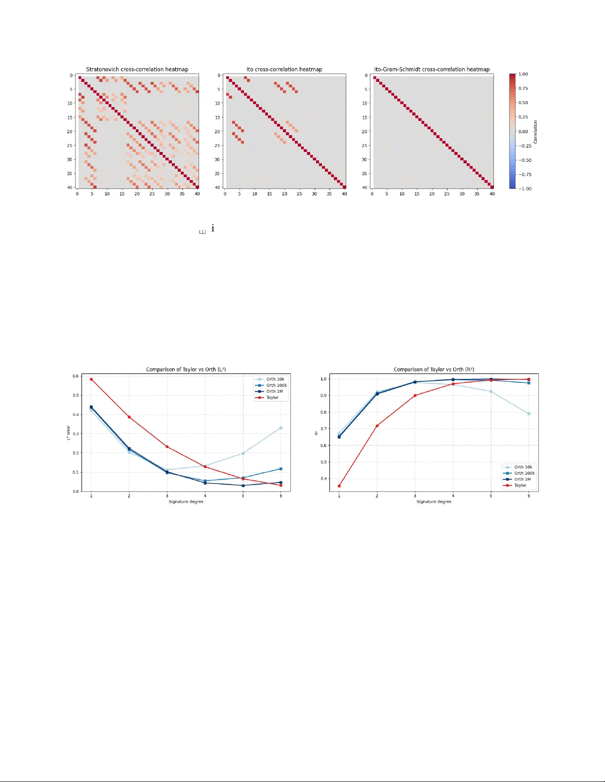
Orthogonal polynomials on path-space Ily a Chevyre v, Emilio Ferrucci, Darrick Lee, T erry L y ons, Harald Oberhauser, and Nikolas T apia A bstract . W e consider the orthogonalisation of the signature of a stochastic process as the analogue of orthogonal polynomials on path-space. Under an infinite radius of conver gence assumption, w e prov e density of linear functions on the signature in L p functions on grouplike elements, making it possible to represent a square-integrable function on (rough) paths as an L 2 -conv ergent series. By viewing the shuffle algebra as commutativ e polynomials on the free Lie algebra, w e revisit much of the theory of classical orthogonal polynomials in sev eral variables, such as the recurrence relation and Fa vard’s theorem. Finally , w e restrict our attention to the case of Bro wnian motion with and without drift, and pro ve that dimension-independent orthogonal signature exists with drift but not without. W e end with numerical examples of how orthogonal signature polynomials of Brownian motion can be applied for the approximation of functions on paths sampled from the W iener measure. February 21, 2026 C ontents 1. Introduction 2 2. L 2 orthogonal signature expansions 5 2.1. Signature of a stochastic process 5 2.2. Orthogonalisation of signature features 6 2.3. Density of linear functions on the signature in L p 8 3. General properties of orthogonal shuffle polynomials 10 3.1. Shuffle polynomials as graded commutativ e polynomials 10 3.2. Recurrence relation 11 3.3. Rank condition 12 3.4. Fa vard’s theorem 14 3.5. Jacobi matrices and measures on b W 16 3.5.1. Background on spectral theor y 17 3.5.2. Commutativity and cyclic v ectors 17 3.5.3. Bounded case 18 3.5.4. Unbounded case 19 3.6. Measures on G ( V ) 20 4. Orthogonal polynomials on W iener space 22 4.1. The non-time-augmented case: non-existence 22 4.2. The time-augmented case: Itô orthogonal polynomials 26 4.3. Numerical experiments 31 References 34 Appendix A. Linear systems 36 1 2 1. Introduction Orthogonal polynomials in one or sev eral variables ha v e applications in numerical analysis [ 59 ], mathematical physics [ 51 ], probability theor y and stochastic processes [ 55 , 60 ], mathematical finance [ 1 ], and in many other areas of mathematics and the applied sciences. One simple example that exhibits their potential is the following. T ake a function f : [ − 1, 1 ] → R . If f is analytic at 0, w e ma y approximate it with its T a ylor polynomials near 0. Outside its radius of conv ergence, how ev er , the T a ylor approximation will not conv erge, and ev en within, it ma y conv erge slowly . On the other hand, as long as f ∈ L 2 [ − 1, 1 ] , its L 2 -projections onto the space spanned b y polynomials of degree N , Π N f , will conv erge to f in L 2 as N → ∞ (and ev en unifor mly if f has Hölder regularity greater than 1 2 [ 53 ]). These projections can be found computing the L 2 inner product ( ℓ n , f ) = R 1 − 1 f ( x ) ℓ n ( x ) d x with the Legendre polynomials, orthogonal w .r .t. the Lebesgue measure on [ − 1, 1 ] and expanding f = ∞ ∑ n = 0 ( ℓ n , f ) ( ℓ n , ℓ n ) ℓ n . (1.1) The series truncated at N coincides with Π N f . A comparison of the tw o types of approximation is giv en in Figure 1 . 1.00 0.75 0.50 0.25 0.00 0.25 0.50 0.75 1.00 x 0.0 0.2 0.4 0.6 0.8 1.0 f(x) T aylor Appr o ximations f n=0 n=1 n=2 n=3 n=4 n=5 1.00 0.75 0.50 0.25 0.00 0.25 0.50 0.75 1.00 x L2 Appr o ximations f n=0,1 n=2,3 n=4,5 F igure 1. T aylor and L 2 approximations (computed with Legendre orthogonal poly- nomials) of f ( x ) = 1 1 + x 2 . Since f has poles at ± i , the T a ylor approximations do not conv erge unifor mly on ( − 1, 1 ) . Since the work of Chen [ 15 ], iterated path integrals S n ( X ) 0, T : = Z 0 < t 1 < . . . < t n < T d X t 1 ⊗ · · · ⊗ d X t n , X : [ 0, T ] → R d ha v e established themselv es as the path-space analogue of polynomials. For rougher signals the y are ill-defined fr om analysis alone, but in some cases can be defined pr obabilistically; specifying the first few subject to certain requirements forms the definition of a rough path [ 42 ], i.e., a specification of a theor y of differ ential equations. The full stack of iterated integrals, its signature S ( X ) 0, T , has been sho wn to characterise the path up to tree-like equivalence , a generalised form of reparametrisation which allo ws “retracings”, see [ 11 , 16 , 33 ] for the proof of this statement in the case of X piecewise regular , bounded v ariation, and rough, respectiv ely . Moreo v er , since coordinate functions on the signature form an algebra under the shuffle pr oduct (see ( 2.3 ) belo w), the Stone-W eierstrass theorem guarantees that, roughly speaking, for any continuous function on a compact set of (rough) paths K and any ε > 0 there exists a truncation lev el N and a linear function λ N of S N ( X ) 0, T (the signature 3 truncated at degree N , see ( 2.2 ) below), such that sup X ∈ K | F ( X ) − ⟨ λ N , S N ( X ) 0, T ⟩ | < ε . (1.2) This result pro ves that functions on paths can be approximately linearised in ter ms of the signature, but has a couple of shortcomings. First of all, most sets of paths on which interesting functions are defined (e.g. the support of the law on path-space of the solution to an SDE [ 56 ], or indeed the support of the la w of Brownian motion itself) are not compact. Secondly , writing λ N = ∑ N k = 0 λ k N with λ k N acting on tensor degree k , it cannot be expected that a linear function λ N ′ ( N ′ > N ) that achiev es a better approximation ( ε ′ < ε ) should ha v e the same low-or der tensor projections: in general λ k N  = λ k N ′ for k ≤ N , i.e. the approximation is not stable under increasing the precision of the approximation. This latter phenomenon is not specific to approximations of the type ( 1.2 ) for signatures and ev en occurs for L 2 -approximations of functions in one variable with polynomials: if f ∈ L 2 [ − 1, 1 ] as abov e, writing ( Π N f )( x ) = ∑ N k = 0 λ k N x k , the same instability occurs, simply because monomials are correlated w .r .t. the Lebesgue measure on [ − 1, 1 ] (or indeed w .r .t. any measure that is not the Dirac delta δ 0 ). Iterated integrals also naturally appear in numerical schemes for stochastic differential equa- tions (SDEs) [ 36 ], see also [ 27 , 40 ] for similar schemes which deal with path-dependency . These approximations are quite different to ( 1.2 ), since they generally rely on the inter val [ 0, T ] being split into many sub-inter v als, and on the expansion to be perfor med on each inter val, for conver gence to be guaranteed. More specifically , an important example of function on paths is φ ( Y T ) , where φ is a smooth function and Y is the solution to the controlled differ ential equation with smooth v ector fields F 1 , . . . , F d ∈ C ∞ ( R n , R n ) : d Y t = F ( Y t ) d X t , Y 0 = y 0 . (1.3) Applying the chain rule N times yields the expansion φ ( Y T ) = φ ( y 0 ) + N ∑ n = 1 ⟨ F α 1 · · · F α n φ ( y 0 ) , S ( X ) α 1 .. . α n 0, T ⟩ + R N ( F , φ , X ) 0, T with R N ( F , φ , X ) 0, T = Z 0 < t 1 < . . . < t N < T F α 1 · · · F α N φ ( Y t 1 ) d X α 1 t 1 · · · d X α N t N . (1.4) Failures of analyticity such as Figure 1 , which a fortiori occur in the path setting (since iterated in- tegrals embed monomials) sho w that this error cannot generally be made small without controlling the size of the inter v al. This type of approximation scheme therefore has the benefit of having ex- plicit identities for the coefficients in the expansion, but the dra wbacks of requiring a more explicit form of the function on paths (e.g. the v ector fields in the differential equation) and of requiring iteration for conver gence. Briefly retur ning to a polynomial L 2 -approximations for functions in one variable, obser v e that a necessar y condition for a representation like ( 1.1 ) to hold is that polynomials be dense in L 2 . This is alwa ys true if the measure is compactly supported, but for general measures on the real line the question of density of polynomials in L p is intimately related to that of moment-determinacy [ 9 ], i.e. whether the measure is unique giv en its moments E µ x n . On path-space, the analogous question asks whether the expected signature E S ( X ) 0, T of a stochastic process deter mines its law . The question w as answ ered in the affirmativ e in [ 19 ] under an “infinite radius of conv ergence” assumption, which holds true for many stochastic processes lifted to rough paths considered in the literature [ 30 ]. The goal of this paper is to combine orthogonal polynomials with path signatures, for ming what w e consider the analogue of orthogonal polynomials on path-space. Our contributions are as follo ws. In S ection 2 w e briefly introduce the signature of a stochastic process and sho w how 4 its canonical coordinates can be (block-)orthogonalised with the familiar Gram-S chmidt procedure, giv en the kno wledge of the expected signature of the process. Next, w e pro ve that, under the same infinite radius of conv ergence assumption as in [ 19 ], linear functions on the signature are dense in L p functions on paths (modulo tree-like equiv alence) for any p ∈ [ 1, ∞ ) . While this result holds under the same hypotheses as in [ 19 ], it does not follo w directly from the latter . Combined with orthogonalisation, our density result yields an L 2 -series expansion for a square integrable function on paths F . This circumv ents both the issues of poor conv ergence aw a y from the point of expansion of ( 1.4 ) and the issues of stability under increase in precision of ( 1.2 ). W e remark that L p -density of signature functionals w as also v er y recently pro v ed in [ 14 ] using w eighted spaces for a class of time-augmented processes. Our density result is, how e v er , stronger 1 and applies without any assumptions bey ond an infinite radius of conv ergence. Our proof is moreov er v ery different from [ 14 ] and follows more the style of the proof of moment determinacy [ 19 ]. In S ection 3 w e begin by obser ving the kno wn fact that a change of basis transfor ms the shuffle algebra, which gov erns the product of coordinate functions on the signature, into the polynomial al- gebra ov er an infinite-dimensional but graded space (the free Lie algebra). This enables us to revisit much of the theor y of classical orthogonal polynomials in sev eral variables [ 25 ], with the added dif- ficulty of infinite dimensionality and anisotropic grading on the base v ariables. W e pro v e v ersions of the celebrated three-term recurrence relation, which is no longer three-ter m but nev ertheless yields a wa y of computing the orthogonal signature polynomials alternatively to Gram-S chmidt. W e also pro v e a version of Fa v ard’s theorem, which characterises which sequences of polynomials arise as orthogonal polynomials with respect to an inner product. W e then study when such inner products arise from probability measures on both the free Lie algebra and path space. In S ection 4 w e specify our study to what is arguably the most important example of stochastic process, Bro wnian motion, seeking more explicit descriptions of the orthogonal signature polyno- mials. W e ask the question of naturality , i.e. roughly speaking whether the orthogonal polynomials associated to a V -valued brownian motion can be expressed without reference to a basis or ev en to the dimension of V . While this is true of ordinary Hermite polynomials in sev eral v ariables, w e pro v e, using symbolic linear algebra code that it is not true for the signature of Brownian mo- tion, unless time is included as a coor dinate. This concer n is not merely motiv ated b y aesthetics, rather , it speeds up the computation of the orthogonal signature compared to naiv ely performing Gram-S chmidt orthogonalisation. W e proceed with the explicit description and computation of or- thogonal signature polynomials of time-augmented Bro wnian motion which are natural (basis- and dimension- free). W e also giv e an independent, short, W iener chaos-based proof of density of linear functions on the signature in L 2 in the time-augmented case. W e end with a description of our implementation [ 17 ] of these orthogonal polynomials on W iener space and show ho w it can be used in approximation problems. W e believ e that, in future w ork, it would be interesting to consider the orthogonal signature associated to the time-augmented stochastic processes (many of which with jumps) associated to the Askey classification [ 3 ], see [ 55 ]. Acknowledgements. W e thank Cris Salvi for many helpful discussions on the topics of this paper . 1 More specifically , [ 14 ] requires time-augmentation and integrability of the w eight w ( X ) = exp ( β ∥ X ∥ N α ) for some β > 0, where N = ⌊ 1 / α ⌋ and ∥ X ∥ α is the α -Hölder homogeneous rough path nor m. Integrability of w (for any β > 0) implies an infinite radius of conver gence of E S ( X ) 0, T , so our Theorem 2.4 implies [ 14 , Thm. 3.4], but not conv ersely since we do not require time augmentation and do not assume integrability of w . For example, Theorem 2.4 applies to fractional Brownian motion with 1 /4 < H ≤ 1 /3 while [ 14 , Thm. 3.4] does not because w is not integrability as in this case N = 3. Moreov er , the restriction to time augmented processes seems important in [ 14 ] since the proof relies on the uniform density result in w eighted spaces from [ 23 ], which appears to use time augmentation in a crucial wa y . 5 IC and EF gratefully ackno wledge support from the ERC via the Starting Grant SQGT 101116964. During the first phase of this project, EF w as employ ed at the University of Oxford and supported by the EPSRC programme grant [EP/S026347/1]. DL w as supported b y the Hong Kong Inno vation and T echnology Commission (InnoHK Project CIMDA) during part of this work. TL w as supported in part by UK Research and Innov ation (UKRI) through the Engineering and Physical S ciences Research Council (EPSRC) via Programme Grants [Grant No. UKRI1010: High order mathematical and computational infrastructure for streamed data that enhance contemporary generativ e and large language mod- els], [Grant No. EP/S026347/1: Unparameterised multi-model data, high order signatures and the mathematics of data science], and the UKRI AI for S cience a ward [Grant No. UKRI2385: Creating Foundational Benchmarks for AI in Phys- ical and Biological Complexity]. He was also supported b y The Alan T uring Institute under the Defence and S ecurity Programme (funded b y the UK Gov ernment) and through the provision of research facilities; by the UK Gov ernment; and through CIMDA@Oxford, part of the AIR@InnoHK initiativ e funded by the Innov ation and T echnology Commis- sion, HKSAR Gov ernment. HO w as supported by [EP/Y028872/1] (An "Erlangen Programme" for AI) and by the Hong Kong Innov ation and T echnology Commission (InnoHK Project CIMDA). NT acknowledges funding by the Deutsche Forschungsgemeinschaft (DFG, Ger man Research Foundation) – CRC/TRR 388 “Rough Analysis, Stochastic Dynamics and Related Fields” – Project ID 516748464. For the pur pose of open access, the authors hav e applied a Creativ e Commons Attribution (CC BY) license to any author accepted manuscript version arising from this submission. 2. L 2 orthogonal signature expansions 2.1. Signature of a stochastic process. Let X be a continuous stochastic process in a time v ari- able on [ 0, T ] taking v alues in the finite-dimensional vector space V , defined on a probability space ( Ω , F , P ) . Let X be of bounded p -variation and let X be a p -geometric rough path lift of X , which w e assume to be F -measurable (this is the case for all the main examples of stochastic rough paths). For a finite-dimensional vector space U w e denote T N ( U ) : = N M m = 0 U ⊗ m , T ( U ) : = ∞ M m = 0 U ⊗ m , T ( ( U ) ) : = ∞ ∏ m = 0 U ⊗ m . (2.1) W e recall that, giv en the rough path lift X , its signature is canonically defined [ 42 ], and represents the iterated integrals S n ( X ) 0, T = Z 0 < t 1 .. . < t n < T d X t 1 ⊗ · · · ⊗ d X t n ∈ V ⊗ n S N ( X ) 0, T = ( S 0 ( X ) 0, T , . . . , S N ( X ) 0, T ) ∈ T N ( V ) S ( X ) 0, T = ( S 0 ( X ) 0, T , . . . , S N ( X ) 0, T , . . . ) ∈ T ( ( V ) ) (2.2) defined according to the integration theory specified by X . W e write ⟨ · , · ⟩ for the canonical dual pairing betw een T ( V ∗ ) and T ( ( V ) ) , e.g. for a w ord w = α 1 . . . α n representing an elementar y tensor in ( V ∗ ) ⊗ n w e ha v e ⟨ w , S ( X ) 0, T ⟩ : = Z 0 < t 1 .. . < t n < T d X α 1 t 1 ⊗ · · · ⊗ d X α n t n . W e write | w | = n for the tensor degree of w . W e recall that signature coordinates satisfy the shuffle identity , i.e. for u , v ∈ T ( V ∗ ) ⟨ u , S ( X ) ⟩ ⟨ v , S ( X ) ⟩ = ⟨ u  v , S ( X ) ⟩ . (2.3) where  is the shuffle product of the tw o wor ds. For this reason w e sometimes will call Sh ( V ∗ ) = T ( V ∗ ) when view ed as an algebra under the shuffle product and correspondingly write Sh N ( V ∗ ) = T N ( V ∗ ) . Elements of T ( ( V ) ) satisfying ( 2.3 ) for m a (formal) group G ( V ) ⊂ T ( ( V ) ) , whose Lie algebra is the space of free Lie series [ 50 ]. Recall that A = ( A 0 , A 1 , . . . ) ∈ T ( ( V ) ) has an infinite radius of 6 convergence if ∥ A ∥ λ : = ∞ ∑ n = 0 ∥ A n ∥ V ⊗ n λ n < ∞ for all λ > 0, (2.4) where we equip V with a norm and V ⊗ n with an arbitrary cross nor m, e.g. the projectiv e nor m (by finite dimensionality of V , condition ( 2.4 ) does not depend on the choice of norms). Denote e T ( ( V ) ) the space of these elements and e G ( V ) : = e T ( ( V ) ) ∩ G ( V ) . W e equip e T ( ( V ) ) with the (locally conv ex) topology giv en b y the nor ms ∥ · ∥ λ , and e G ( V ) inherits this topology , making it a topological group, and a Polish (completely metrisable and separable) space [ 19 ]. It is a fact that S ( X ) 0, T is an element of e G ( V ) for any rough path X , see e.g. [ 43 ]. Therefore, w e ma y view the stochastic process X as defining a probability measure on e G ( V ) . From now on, unless there is an ambiguity as to the rough path lift X , w e will drop the bold font and simply write S ( X ) 0, T and similar; we will alwa ys use X to denote the trace of X , i.e. its projection onto V . The signature encodes almost all the infor mation in the (rough) path, namely up to tree-like equiv alence [ 11 , 16 , 33 ], a generalised for m of reparametrisation that includes “retracings”. A com- mon wa y of ensuring the path is tree-reduced, and thus that the full path can be reco v ered from the signature, is to include time as a coor dinate, see e.g. [ 29 ]. W e let G denote the sigma-algebra generated by S ( X ) 0, T . R emark 2.1 ( G = F ). If time is included as zero-th coordinate of X , it follo ws from the fact that X is tree-reduced (i.e. t 7 → X 0, t is injective) and measurability of the map that reconstructs the tree-reduced representativ e from the signature [ 32 ], that G = F . In many cases of interest, such as Bro wnian motion [ 37 ] and the la w of certain multidimensional diffusions [ 31 ], G = F ev en without including time as a coordinate of the process. 2.2. Orthogonalisation of signature features. W e assume that ⟨ w , S ( X ) 0, T ⟩ ∈ L 2 ( G ) for all w ∈ Sh ( V ∗ ) . Define the positiv e semi-definite symmetric bilinear for m ( u , v ) : = E ⟨ u , S ( X ) 0, T ⟩ ⟨ v , S ( X ) 0, T ⟩ = ⟨ u  v , E S ( X ) 0, T ⟩ . (2.5) This bilinear form is, in general, only positive semi-definite because the natural map ϕ : Sh N ( V ∗ ) → L 2 ( G ) is not in general an inclusion. Let N be its nullspace and W a choice of a direct complement to it, so that Sh ( V ∗ ) = N ⊕ W and ϕ embeds W into L 2 ( G ) . W e may alwa ys choose W to be of the for m W = L ∞ n = 0 W n with W n ⊂ ( V ∗ ) ⊗ n : indeed, let W n be the pre-image through the quotient π : Sh ( V ∗ ) ↠ Sh ( V ∗ ) / N of some basis of π ( ( V ∗ ) ⊗ n ) and take W n = span ( W n ) . As usual call W n = F n k = 0 W k the basis of W n = L n k = 0 W k . Let Π N : L 2 ( G ) ↠ span { ⟨ ℓ , S ( X ) 0, T ⟩ | ℓ ∈ Sh N ( V ∗ ) } Π n : L 2 ( G ) ↠ span { ⟨ ℓ , S ( X ) 0, T ⟩ | ℓ ∈ ( V ∗ ) ⊗ n } 1 − Π N = : Π ⊥ N : L 2 ( G ) ↠ span { ⟨ ℓ , S ( X ) 0, T ⟩ | ℓ ∈ Sh N ( V ∗ ) } ⊥ (2.6) denote orthogonal projections, where ⊥ denotes the orthogonal complement in L 2 ( G ) . W e consider the block-orthogonalisation map p p : W ∼ = − → W , p | W n = Π ⊥ n − 1 | W n , w 7 → p w . (2.7) Notice that p | W n takes v alues in W n − 1 ⊕ W n = W n and therefore so does p | W n , i.e. p is triangular , and moreo v er monic, namely Π n ◦ p | W n = 1 . It can be computed by solving, for w ∈ W n (and extended 7 linearly to W n ) p w = w − ∑ u ∈ W n − 1 λ u u ,  w − ∑ u ∈ W n − 1 λ u u , v  = 0 for v ∈ W n − 1 . (2.8) Let V be a basis of V ∗ , then the w ords α 1 . . . α n in V n define a basis of Sh ( V ∗ ) , and write V • : = F n ∈ N ( V ∗ ) ⊗ n . If the bilinear form ( · , · ) is positiv e-definite, then W = Sh ( V ∗ ) ; in many cases it is possible to realise W n as the linear span of a subset of V • (see S ection 4.2 below for an explicit example of this). Assume this is the case, and that W n is a subset of w ords in V n . W e then call the elements { p w } w ∈ W the block-orthogonal shuffle polynomials since ( p v , p w ) = 0 for v , w ∈ W with | v |  = | w | . Assume furthermore the basis W is totally ordered in a w a y that respects the grading ( v < w if | v | < | w | ). W e ma y then define a fully orthogonal basis b y the Gram-S chmidt orthogonalisation procedure: e p w : = w − ∑ v ∈ W • v < w ( e p v , e p v ) > 0 ( w , e p v ) ( e p v , e p v ) e p v (2.9) where v < w if | v | < | w | or if | v | = | w | and v < w lexicographically . Then { e p w } w ∈ W n is an orthogonal basis of span { p w | w ∈ W n } . In the next subsection w e will identify a large class of stochastic processes for which linear functions on S ( X ) 0, T are dense in L p ( G ) . W e view the next two results as corollaries of that result. C orollary 2.2 (Learning F ( X ) b y linear regression). Let Y = F ( X ) ∈ L 2 ( G ) and { ( X i , Y i = F ( X i ) + ε i } M i = 1 be an i.i.d. sample of input-output pairs, where ε i are i.i.d. err ors independent of X . Let Φ ∈ R M × D be the data matrix with Φ i v = ⟨ p v , S N ( X ) 0, T ⟩ , i = 1, . . . , M ; v ∈ V n with n ≤ N and D = D ( d , N ) = d N + 1 − 1 d − 1 the dimension of T N ( R d ) . Then the estimator for ordinary least squares (OLS) b β = ( Φ ⊺ Φ ) − 1 Φ ⊺ Y = Φ ⊺ ( Φ Φ ⊺ ) − 1 Y (2.10) is such that ⟨ b β , S N ( X ) 0, T ⟩ converges in L 2 to Π N Y as M → ∞ . Its entries converge (in blocks) to Π n Y , and are thus asymptotically stable under increasing degree N . Therefor e, under the hypotheses of Theorem 2.4 below , Y can be estimated arbitrarily well by OLS linear regr ession on the truncated signature. W e refer to the standard literature on statistical lear ning (e.g. [ 5 , Ch. 3]) for more general state- ments that imply its proof. In most real-w orld cases in which data is limited it is desirable or ev en necessary to use ridge or lasso regression; consistency results could be for mulated for these too, by letting the regularisation parameter vanish in the large data limit. Consistency of the OLS estimator and the statement about univ ersality of OLS estimation of course holds true without any orthog- onalisation, since the projection Π N does not depend on it. How e ver , as explained in S ection 1 , orthogonalisation is necessar y to obtain a series representation. The following is classical. C orollary 2.3 (S eries expansion of an L 2 function on paths). Under the hypotheses of Theorem 2.4 below , for Y ∈ L 2 ( G ) Y = ∞ ∑ n = 0 Π n Y = ∑ v : ( e p v , e p v ) > 0 ⟨ ℓ Y v , S ( X ) 0, T ⟩ , ℓ Y v : = E [ Y ⟨ e p v , S ( X ) 0, T ⟩ ] ( e p v , e p v ) e p v with Π n defined in ( 2.6 ) , e p v in ( 2.9 ) , and convergence of the series in L 2 . 8 P roof . Π N = ∑ N n = 0 Π n and by density ∥ Y − Π N Y ∥ L 2 → 0. The second equality follo ws by further decomposing Π n into the projections onto the orthogonal directions spanned by the v ectors e p I . □ 2.3. Density of linear functions on the signature in L p . The goal of this section is to prov e the following result. W e equip R d with the ℓ 1 norm ∥ ( x 1 , . . . , x d ) ∥ = ∑ d i = 1 | x i | and equip all tensor products, including ( R d ) ⊗ k , with the projectiv e tensor nor m. T heorem 2.4. Consider a probability measure µ on e G ( R d ) with infinite radius of convergence, i.e. ∞ ∑ k = 0 λ k ∥ E S ∼ µ S k ∥ ( R d ) ⊗ k < ∞ for all λ > 0 . (2.11) Then the space of linear coordinate functions on e G ( R d ) are dense in L p ( µ ) for all p ∈ [ 1, ∞ ) . The exact choice of nor ms on ( R d ) ⊗ k for k ≥ 1 is not important in Theorem 2.4 because if µ v erifies ( 2.11 ) for one choice of nor ms, then it v erifies ( 2.11 ) for all choices of cross norms. As w e discuss in S ection 1 , a related L p -density result, which is more restrictiv e as it requires time to be included as a coordinate and a w eight function to be integrable, has v er y recently been obtained in [ 14 ]. S ee also Proposition 4.10 below for a short W iener chaos-based proof that applies in the case p = 2 and X is a time-augmented Bro wnian motion. Theorem 2.4 applies to the sto- chastic processes to which the moment-determinacy results of [ 19 ] applies to, such as Gaussian and Marko vian rough paths. Note that, while the hypothesis of infinite radius of conv ergence is the same as in [ 19 ], L p density does not follo w from moment determinacy alone: this is ev en true in finite dimension [ 10 ] (only in the scalar case and p ≤ 2 does this implication hold [ 25 , p.69]). W e also remark that a similar approximation r esult for the modified robust signatures [ 20 ] w as obtained in [ 7 ]. For the proof, w e requir e a few lemmas. In the follo wing, let ( Y , ρ ) be a complete (not necessarily separable) metric space with a Borel probability measure µ . L emma 2.5. The space of continuous bounded functions is dense in L p ( µ ) for any p ∈ [ 1, ∞ ) . P roof . The span of indicator functions on open sets is dense in L p ( µ ) . But for A ⊂ Y open, the continuous bounded function f n ( y ) = { n inf x ∈ Y \ A ρ ( x , y ) } ∧ 1 conv erges to 1 A pointwise, and thus in L p b y dominated conv ergence. □ W e sa y that a set of functions A ⊂ R Y separates points if for all distinct x , y ∈ Y there exists h ∈ A such that h ( x )  = h ( y ) . L emma 2.6. Suppose A is an algebra of continuous bounded functions on Y that separates points and contains the constant functions. Suppose also that µ is Radon (which is automatic if Y is separable). Then A is dense in L p ( µ ) for any p ∈ [ 1, ∞ ) . P roof . There are sev eral proofs, see e.g. [ 24 ] for an ev en stronger statement that drops the con- tinuity assumption. W e giv e here an elementary proof that uses only the classical Stone–W eierstrass theorem. W e let C > 0 denote a sufficiently large univ ersal constant. Let A be the closure of A in L p ( µ ) . By Lemma 2.5 , it suffices to show that if f : Y → R is continuous with sup y ∈ Y | f ( y ) | ≤ 1, then for ev ery ε > 0, there exists h ∈ A such that | f − h | L p ( µ ) < ε . T o this end, consider ε ∈ ( 0, 1 ) . Let K ⊂ Y be a compact set such that µ ( Y \ K ) < ε ; such a set K exists because µ is Radon. By Stone–W eierstrass, there exists g ∈ A such that sup y ∈ K | g ( y ) − f ( y ) | < ε (of course g depends on K and f ). At this stage, w e don’ t hav e | g − f | L p ( µ ) small because g might be large outside K . 9 No w consider the functions h δ ( y ) = e − δ g ( y ) 2 g ( y ) for small δ > 0. Define H ( δ ) = sup x ∈ R | e − δ x 2 x | . Then H ( δ ) ≤ C δ − 1/ 2 and thus sup y ∈ Y | h δ ( y ) | ≤ H ( δ ) ≤ C δ − 1/ 2 . Moreo v er sup y ∈ K | g ( y ) − h δ ( y ) | ≤ C δ since sup y ∈ K | g ( y ) | ≤ 2 and e − δ z 2 = 1 + O ( δ z 2 ) for | z | ≤ 2. In particular , sup y ∈ K | f ( y ) − h δ ( y ) | ≤ ε + C δ and thus Z K | f − h δ | p d µ ≤ ( ε + C δ ) p . On the other hand, Z Y \ K { f p + h p δ } d µ ≤ ε + ε H ( δ ) p ≤ ε + C p ε δ − p /2 T aking δ = ε 1/ p , we obtain ∥ f − h δ ∥ p L p ( µ ) ≤ ( ε + C ε 1/ p ) p + ε + C p ε 1/2 . It remains to sho w that h δ ∈ A . W e write as a po w er series h δ = ∑ ∞ n = 0 ( − δ ) n g 2 n + 1 n ! and remark that, since g is bounded on Y , the series conv erges absolutely in L p . Since g n ∈ A for all n ≥ 1, w e obtain h δ ∈ A . □ P roof of T heorem 2.4 . Let A denote the space of matrix coefficients of unitary representations of e G ( R d ) as in [ 19 ], i.e. A contains those functions f : e G ( R d ) → C such that f ( S ) = ⟨ M ( S ) u , v ⟩ C N for some u , v ∈ C N and a linear map M : R d → u ( N ) for some N ≥ 1, where u ( N ) is the space of N × N skew-Hermitian matrices and where M ( S ) = ∑ ∞ k = 0 M ⊗ k S k , which is a unitar y N × N matrix. Then A is a C -algebra of bounded continuous functions on e G ( R d ) which, b y [ 19 , Theorem 4.8] (see also [ 39 ] for a different proof), separates points. Moreo v er A contains the constant functions and is closed under complex conjugation, so by Lemma 2.6 , functions of the for m ℜ f for f ∈ A are dense in L p ( µ ) . It remains to show that ev ery f ∈ A can be approximated in L p ( µ ) b y ( C -valued) linear functions on e G ( R d ) . Consider a map M : R d → u ( N ) and let S = ( 1, S 1 , S 2 , . . . ) be a e G ( R d ) -valued random v ariable with law µ . Since ∑ n k = 0 M ⊗ k S k is a linear function on e G ( R d ) and M ( S ) = ∑ ∞ k = 0 M ⊗ k S k , it suffices to sho w that lim n → ∞ ∞ ∑ k = n ∥ M ∥ k ( E ∥ S k ∥ p ( R d ) ⊗ k ) 1/ p = 0 . (2.12) For nor med spaces E , F , w e equip E ⊕ F with the ℓ 1 norm ∥ ( x , y ) ∥ = ∥ x ∥ E + ∥ y ∥ F . Consider no w n ≥ 2 and the n -th iterated copr oduct ∆ n : T ( R d ) → T ( R d ) ⊗ n , which is the unique algebra morphism giv en b y ∆ n ( v ) = v ⊗ 1 ⊗ · · · ⊗ 1 + · · · + 1 ⊗ · · · 1 ⊗ v for v ∈ R d , where the number of ter ms is n (see [ 50 , S ec. 1.4]). Note that ∆ 2 = ∆ is the usual coproduct on T ( R d ) which is dual to the shuffle product. In particular , for v ∈ R d , ∥ ∆ n v ∥ ( R d ) n = n ∥ v ∥ R d (2.13) and thus, for x ∈ ( R d ) ⊗ k , ∥ ∆ n x ∥ ≤ n k ∥ x ∥ ( R d ) ⊗ k . (2.14) Here, ∆ n x is an element in L k 1 + . . . + k n = k N n i = 1 ( R d ) ⊗ k i , which w e recall is equipped with the ℓ 1 norm of the corresponding projectiv e tensor nor ms. The bound ( 2.14 ) follows from ( 2.13 ) and the fact that, for any nor med algebra B and linear map Q : R d → B with operator nor m ∥ Q ∥ , Q ⊗ k : ( R d ) ⊗ k → B 10 has operator norm bounded abov e by ∥ Q ∥ k due to the choice of projectiv e nor ms on ( R d ) ⊗ k . More precisely , w e apply this with Q = ∆ n , for which ∥ Q ∥ = n b y ( 2.13 ), and B = T ( R d ) ⊗ n equipped with the projectiv e nor m, where w e equip T ( R d ) with the ℓ 1 norm ∥ ( x 0 , x 1 , . . . ) ∥ = ∑ k ≥ 0 ∥ x k ∥ ( R d ) ⊗ k . Therefore, for p ≥ 1 an integer , using the duality betw een shuffle and ∆ as in [ 50 , Sec. 1.5] and the fact that S takes values in G ( R d ) , E ∥ S k ∥ 2 p ( R d ) ⊗ k = E  ∑ | w | = k | ⟨ w , S k ⟩ |  2 p ≤ d k ( 2 p − 1 ) ∑ | w | = k E ⟨ w , S k ⟩ 2 p = d k ( 2 p − 1 ) ∑ | w | = k E ⟨ w  2 p , S 2 pk ⟩ = d k ( 2 p − 1 ) ∑ | w | = k E ⟨ w ⊗ 2 p , ∆ 2 p S 2 pk ⟩ ≤ d k ( 2 p − 1 ) ∥ ∆ 2 p E S 2 pk ∥ ≤ d k ( 2 p − 1 ) ( 2 p ) 2 pk ∥ E S 2 pk ∥ ( R d ) ⊗ 2 p k , where w in the sums ranges ov er all w ords of length k in the canonical basis of R d (this generalises the calculation abov e [ 19 , Proposition 3.4] which was for p = 1). Since E S has an infinite radius of conv ergence, for any ε > 0, one has ∥ E S k ∥ ≤ ε k for all k > k ( ε ) ≥ 1 sufficiently large. Therefore, for all k > k ( ε ) , ( E ∥ S k ∥ 2 p ) 1/ ( 2 p ) ≤ d k ( 2 p − 1 ) 2 p ( 2 p ) k ε k . T aking ε sufficiently small (depending on ∥ M ∥ , p , and d ), w e obtain ( 2.12 ) as required. □ 3. General properties of orthogonal shuffle polynomials In this section, w e discuss structural properties of orthogonal shuf fle polynomials in Sh ( V ∗ ) , generalizing sev eral classical results in the classical commutativ e setting. W e begin by refor mulating shuffle polynomials as ordinary commutativ e polynomials with graded generators. 3.1. Shuffle polynomials as graded commutativ e polynomials. For a v ector space V , let Sym ( V ) denote the symmetric algebra of V . Recall that L ( V ) denotes the free Lie algebra of V and, from [ 50 ], Sh ( V ∗ ) = Sym ( L ( V ) gr ) (3.1) as commutative algebras, where ( · ) gr denotes the graded dual and identity is intended as being betw een functors. Fixing a Hall basis of L ( V ) allows us to express elements of Sh ( V ∗ ) as polyno- mials ov er an infinite set of indeter minates, specified b y the dual Hall basis [ 50 , §5.2]. As many of the results in this section do not rely on the Lie algebra structure, w e will mainly w ork with a general graded v ector space W = L ∞ m = 0 W m of finite type, where the degree m subspace W m is finite dimensional. Our general results for Sym ( W gr ) apply to the signature setting by taking W = L ( V ) . W e fix a basis of W m , denoted { w m , i } N m i = 1 , where N m is the dimension of W m . W e abuse notation, and also denote the dual basis in ( W m ) ∗ b y w m , i . In general, w e will denote a monomial in Sym ( W gr ) b y w α , where α = ( α m , i ) m ∈ N , i ∈ [ N m ] , where each α m , i ∈ N , and only finitely many are nonzero, and set w α = ∞ ∏ m = 1 N m ∏ i = 1 w α m , i m , i . (3.2) Let Q ∈ Sym ( W gr ) be a polynomial Q = ∑ α q α w α , where finitely many of the b α are nonzero. W e ha v e tw o notions of degree called the tensor (total) degree and the shuffle degree , respectiv ely defined on a shuffle monomial w α b y tdeg ( w α ) = | α | = ∞ ∑ m = 1 N m ∑ i = 1 m α m , i and sdeg ( w α ) = ∞ ∑ m = 1 N m ∑ i = 1 α m , i . 11 W e denote the column v ector of shuffle monomials of total degree n b y w n and denote its dimension b y r n . D efinition 3.1. A linear functional L : Sym ( W gr ) → R is quasi-definite if there exists a basis of Sym ( W gr ) such that for any tw o basis elements P , Q , w e hav e L ( P Q ) = 0 if P  = Q and L ( P 2 )  = 0. If in addition, L satisfies L ( P 2 ) > 0, then w e sa y that L is positiv e-definite. Giv en a quasi-definite functional L , define the symmetric bilinear form (or inner product, if L is positive-definite) ( P , Q ) : = L ( P Q ) , and sa y that { p n } n ≥ 0 , where p n ∈ Sym ( W gr ) r n is block orthogonal if ( w m , p ⊺ n ) = 0 for all m < n and ( w n , p ⊺ n ) is inv ertible. In this section, orthogonal polynomials refer to block orthogonal polynomials. W e say that { e p n } n ≥ 0 is orthonormal if in addition, ( e p n , e p ⊺ n ) is the identity . W e note that there are tw o main differences from the classical orthogonal polynomial setting: (1) there are an infinite number of generators, ie. W is infinite-dimensional; and (2) the generators are graded , and thus orthogonalize with respect to the total degree. In the following subsections, w e generalize classical results about orthogonal polynomials [ 25 ] to our graded, infinite-dimensional setting. W e show that orthogonal polynomials on Sym ( W gr ) satisfy a recurrence relation along with rank conditions on the defining matrices. In S ection 3.4 , w e pro v e the conv erse in a generalization of Fav ard’s theorem, and further more discuss when inner products on Sym ( W gr ) are induced by probability measures in S ection 3.5 . W e retur n to the specific case of W = L ( V ) in S ection 3.6 and discuss measures on G ( V ) . 3.2. Recurrence relation. W e begin by assuming that L is a quasi-definite linear functional on Sym ( W gr ) and that { p n } n ≥ 0 denotes a system of block orthogonal polynomials. Let H n = ( p n , p ⊺ n ) ∈ Mat ( r n , r n ) which is symmetric and invertible by definition of block orthogonality . W e begin by generalizing the three-ter m relation of [ 25 , Theorem 3.3.1] to the graded setting. P roposition 3.2. For n ∈ N 0 , m ∈ [ n ] , i ∈ [ N m ] and − m ≤ k ≤ m, there exist unique matrices M k n , m , i ∈ Mat ( r n − m , r n − m + k ) such that w m , i p n − m = m ∑ k = − m M k n , m , i p n − m + k . (3.3) These matrices satisfy M k n , m , i H n − m + k = H n − m ( M − k n + k , m , i ) ⊺ . (3.4) P roof . The components of w m , i p n − m are polynomials of degree n , so they can be written as a linear combination of orthogonal polynomials, w m , i p n − m = n ∑ k = 0 M k n , m , i p k . Next, due to the orthogonality of polynomials, w e hav e ( w m , i p n − m , p ⊺ k ) = ( M k n , m , i ( p k , p ⊺ k ) : k = n − 2 m , . . . , n 0 : k < n − 2 m . (3.5) 12 The second case is trivial since w m , i p ⊺ k is at most degree k + m ≤ n − m and ( w m , i p n − m , p ⊺ k ) = ( p n − m , w m , i p ⊺ k ) = 0 Therefore, w e hav e M k n , m , i = ( ( w m , i p n − m , p ⊺ k ) H − 1 k : k = n − 2 m , . . . , n 0 : k < n − 2 m . (3.6) Furthermore, for k = n − 2 m , . . . , n , w e hav e M k n , m , i H k = ( w m , i p n − m , p ⊺ k ) = ( w m , i p k , p ⊺ n − m ) ⊺ = H n − m ( M n − m k + m , m , i ) ⊺ . Then we reindex by k 7 → n − m + k to get the result. □ Rather than the classical three ter m recurrence, w e now obtain a recurrence relation with 2 m + 1 terms for degree m generators. This is due to the fact that multiplication b y w m , i increases the degree b y m , and thus ( w m , i p n − m , b p ⊺ k ) ma y be non-trivial for a larger range of degrees k , see ( 3.5 ). Here, ( 3.4 ) provides relationships between matrices for different orders of n . T w o of these will be of particular importance, and we will rename them as A n , m , i : = M m n , m , i ∈ Mat ( r n − m , r n ) and C n , m , i : = M − m n + m , m , i ∈ Mat ( r n , r n − m ) , (3.7) which are related through ( 3.4 ) by A n , m , i H n = H n − m C ⊺ n , m , i . (3.8) In particular , A n , m , i is the leading matrix in the recurrence relation for w m , i p n − m , while C n , m , i is the non-leading matrix in the recurrence for w m , i p n which relates to A n , m , i via ( 3.8 ). S o far , w e hav e been w orking with a block orthogonal system of polynomials p n . How ev er , if the system of polynomials is orthonormal , which w e denote by e p n , then H n = I is the identity matrix, and w e obtain the follo wing. C orollary 3.3. Let e p n be an orthonormal system of polynomials. For n ∈ N 0 , m ∈ [ n ] , i ∈ [ N m ] and 0 ≤ k ≤ m, there exist unique matrices M k n , m , i ∈ Mat ( r n − m , r n − m + k ) for such that w m , i p n − m = m ∑ k = 0 M k n , m , i e p n − m + k + m ∑ k = 1 ( M k n − k , m , i ) ⊺ e p n − m − k . (3.9) Furthermore, M n − m n , m , i is symmetric. P roof . This is immediate from Proposition 3.2 since H n = I is the identity for all n . □ 3.3. Rank condition. Now , we will consider rank conditions that the matrices A n , m , i and C n , m , i must satisfy . W e will consider column joint matrices , which stack a set of matrices in a column. For fixed n ∈ N , suppose { Q n , m , i } m ∈ [ n ] , i ∈ [ N m ] is a set of matrices where Q n , m , i is of size ( p m , q ) , then w e define Q n , m : =      Q n , m ,1 Q n , m ,2 . . . Q n , m , N m      and Q n : =      Q n ,1 Q n ,2 . . . Q n , n      . (3.10) 13 Here Q n , m ∈ Mat ( N m p m , q ) and Q n ∈ Mat ( K , q ) , where K = ∑ n m = 1 N m p m . One particular joint matrix that will be important is A n ∈ Mat ( R n , r n ) , built from A n , m , i ∈ Mat ( r n − m , r n ) , where R n = n ∑ k = 1 N k · r n − k . (3.11) Let G n ∈ Mat ( r n , r n ) be the leading-coefficient matrix of p n ; that is, the matrix G n such that 2 p n = G n w n + q , (3.12) where w n consist of total degree n monomials, and q has total degree strictly less than n . Next, let L n , m , i ∈ Mat ( r n − m , r n ) defined by L n , m , i w n = w m , i · w n − m . L emma 3.4. For each n ∈ N 0 , m ∈ [ n ] and i ∈ [ N m ] , the matrix L n , m , i satisfies L n , m , i · L ⊺ n , m , i = I . Moreover , rank ( L n , m , i ) = r n − m and rank ( L n ) = r n . P roof . By definition, each ro w of L n , m , i has exactly one element equal to 1; other wise the ele- ments are 0. Thus, w e hav e L n , m , i · L ⊺ n , m , i = I and rank ( L n , m , i ) = r n − m . Now , let N n : = { α ∈ N N ≤ n 0 : | α | = n } and N n , m , i : = { α ∈ N n : α m , i  = 0 } , where the α denotes a graded exponent v ector . Then, let a = ( a α ) α ∈ N n ∈ Mat ( r n , 1 ) be a column v ector . Then, L n , m , i is a map which projects a onto its restriction onto N n , m , i . No w , if L n a = 0, then L n , m , i a = 0 for all m ∈ [ n ] and i ∈ [ N m ] . How e ver , since ∪ m , i N n , m , i = N n , w e ha v e a = 0, so L n has full rank. □ Next, for fixed n ∈ N , w e compare the leading coefficient matrices on each side of ( 3.3 ) to get G n − m L n , m , i = A n , m , i G n (3.13) for any m ∈ [ n ] and i ∈ [ N m ] . P roposition 3.5. For each n ∈ N , m ∈ [ n ] and i ∈ [ N m ] , rank ( A n , m , i ) = rank ( C n , m , i ) = r n − m . (3.14) Let A n ∈ Mat ( R n , r n ) be the joint matrix of A n , m , i and C ⊺ n ∈ Mat ( R n , r n ) be the joint matrix of C ⊺ n , m , i ∈ Mat ( r n − m , r n ) . Then, rank ( A n ) = rank ( C ⊺ n ) = r n . (3.15) P roof . From ( 3.13 ) and since all G n are inv ertible, rank ( A n , m , i ) = r n − m from Lemma 3.4 . Fur- thermore, since H n is invertible, we also hav e rank ( C n , m , i ) = r n − m from ( 3.4 ). No w , w e define G m : = G ⊕ N n − m m ∈ Mat ( N n − m r m , N n − m r m ) and G : = G n − 1 ⊕ . . . ⊕ G 0 ∈ Mat ( R n , R n ) . (3.16) 2 Note that these are leading coefficients in terms of the shuffle monomials (with respect to total degree). Thus, ev en for the monic polynomials defined b y Gram-S chmidt in ( 2.9 ), G is not necessarily the identity . 14 Let L n ∈ Mat ( R n , r n ) be the joint matrix of L n , m , i . Then, from ( 3.13 ) and the definition of the joint matrix A n from ( 3.10 ), w e hav e G L n = A n G n , written out in matrix for m as G L n =      G n − 1 0 . . . 0 0 G n − 2 . . . 0 . . . . . . . . . . . . 0 0 . . . G 0           L n ,1 L n ,2 . . . L n , n      =      A n ,1 A n ,2 . . . A n , n      G n = A n G n (3.17) Note that G is inv ertible and thus rank ( A n ) = rank ( L n ) = r n . Next, w e define H m : = H ⊕ N n − m m ∈ Mat ( N n − m r m , N n − m r m ) and H : = H n − 1 ⊕ . . . ⊕ H 0 ∈ Mat ( R n , R n ) . (3.18) Then, ( 3.8 ) implies A n H n = H C ⊺ n . Because H is inv ertible, w e get rank ( C ⊺ n ) = rank ( A n ) = r n . □ Because the matrix A n has full rank, there exists a generalized left inv erse D ⊺ n ∈ Mat ( r n , R n ) , which is expressed as the ro w joint matrix of D ⊺ n , m , i ∈ Mat ( r n , r n − m ) . More explicitly , D ⊺ n , m : =  D ⊺ n , m ,1 . . . D ⊺ n , m , N m  and D ⊺ n : =  D ⊺ n ,1 . . . D ⊺ n , n  . This generalized left inverse (which may not be unique) satisfies D ⊺ n A n = n ∑ m = 1 N m ∑ i = 1 D ⊺ n , m , i · A n , m , i = I ∈ Mat ( r n , r n ) . (3.19) P roposition 3.6. Let D ⊺ n be a generalized inverse of A n . Then, p n = n ∑ m = 1 N m ∑ i = 1 w m , i D ⊺ n , m , i p n − m − m − 1 ∑ k = − m D ⊺ n , m , i M k n , m , i p n − m + k ! P roof . W e multiply the relation from ( 3.3 ) b y D ⊺ n , m , i to get w m , i D ⊺ n , m , i p n − m = D ⊺ n , m , i A n , m , i p n + m − 1 ∑ k = − m D ⊺ n , m , i M k n , m , i p n − m + k . Next, we sum ov er m ∈ [ n ] and i ∈ [ N m ] to get n ∑ m = 1 N m ∑ i = 1  w m , i D ⊺ n , m , i p n − m  = n ∑ m = 1 N m ∑ i = 1 D ⊺ n , m , i A n , m , i ! p n + n ∑ m = 1 m − 1 ∑ k = − m N m ∑ i = 1 D ⊺ n , m , i M k n , m , i ! p n − m + k . Then, applying ( 3.19 ), we obtain the desired result. □ 3.4. Fav ard’ s theorem. In the previous sections, w e sho w ed that giv en a quasi-definite func- tional on Sym ( W gr ) , orthogonal polynomials satisfy a recurrence relation where the defining ma- trices must satisfy certain rank conditions. Her e, w e will pro v e the conv erse: a generalization of Fa var d’s theorem. T heorem 3.7. Let p = { p n } ∞ n = 0 be an arbitrary sequence where p n ∈ Sym ( W gr ) r n is a column vector of length r n , and p 0 = 1 . Then, the following statements are equivalent. (1) There exists a quasi-definite L under which { p n } ∞ n = 0 is a block orthogonal basis in Sym ( W gr ) . (2) For n ∈ N 0 , m ∈ [ n ] , i ∈ [ N m ] and − m ≤ k ≤ m, there exist M k n , m , i ∈ Mat ( r n − m , r n − m + k ) where (a) the polynomials p n satisfy the relation in ( 3.3 ) , and (b) the matrices A n , m , i : = M m n , m , i and C n , m , i : = ( M − m n + m , m , i ) ⊺ satisfy ( 3.14 ) and ( 3.15 ) . P roof . The for w ard direction is giv en by Propositions 3.2 and 3.5 . W e will now prov e the conv erse direction. 15 p is a basis. T o begin, w e must sho w that p for ms a basis of Sym ( W gr ) ; it suf fices to sho w that the leading coefficient matrix G n of p n is inv ertible. Because the polynomials satisfy the relation in ( 3.3 ), the leading coefficient matrices satisfy G L n = A n G n from ( 3.17 ) (and using the same definition of G from there). W e will now show that G n is inv ertible b y induction. For n = 0, w e ha ve p 0 = 1, so G 0 = 1. No w , suppose G 0 , . . . , G n − 1 are inv ertible. By the definition of G in ( 3.16 ), this implies that G is invertible. Therefore, w e ha v e rank ( A n G n ) = rank ( G L n ) = rank ( L n ) = r n , b y Lemma 3.4 . Then, using the rank hypothesis of rank ( A n ) = r n , and the rank inequality for product matrices, w e hav e rank ( G n ) ≥ rank ( A n G n ) ≥ rank ( A n ) + rank ( G n ) − r n = rank ( G n ) . Thus, rank ( G n ) = rank ( A n G n ) = r n , so G n is invertible. p is block orthogonal. Because p is a basis of Sym ( W gr ) , w e can define L : Sym ( W gr ) → R b y L ( 1 ) = 1, L ( p n ) = 0 for n ≥ 1. No w , w e will show that p is block orthogonal with respect to this linear functional. In particular , w e will use induction to sho w that L ( p k p ⊺ j ) = 0 for k  = j . (3.20) Suppose ( 3.20 ) holds for k , j such that 0 ≤ k ≤ n − 1 and j > k . Note that this holds by definition when n = 1. No w , w e note that Proposition 3.6 only used the recurrence in ( 3.3 ) and the rank condition in ( 3.15 ). Thus, for ℓ > n , w e ha v e L ( p n p ⊺ ℓ ) = L n ∑ m = 1 N m ∑ i = 1 w m , i D ⊺ n , m , i p n − m p ⊺ ℓ ! = L n ∑ m = 1 N m ∑ i = 1 D ⊺ n , m , i p n − m m ∑ k = − m M k ℓ + m , m , i p ℓ + k ! ⊺ ! = 0, where w e use Proposition 3.6 and the induction hypothesis in the first equality , the relation in ( 3.3 ) on w m , i p ⊺ ℓ in the second, and the induction hypothesis in the third. Thus, ( 3.20 ) holds. L is nondegenerate. Now , w e will show that H n = L ( p n p ⊺ n ) is inv ertible. First, w e note that H n is symmetric b y definition. Next, by block orthogonality , ( 3.6 ) holds, and therefore ( 3.8 ) also holds. No w , using the definition of H from ( 3.18 ), w e ha v e A n H n = H C ⊺ n . (3.21) W e will once again show that H n is invertible b y induction. Because L ( 1 ) = 1, we ha v e H 0 = 1, which is inv ertible. No w , suppose that H 0 , . . . , H n − 1 is inv ertible, which implies that H is inv ertible. Then, using the rank condition rank ( C ⊺ n ) = r n from ( 3.15 ) by hypothesis, we hav e rank ( A n H n ) = rank ( H C ⊺ n ) = rank ( C ⊺ n ) = r n Then, using the rank inequality for product matrices and the rank condition for A n again, rank ( H n ) ≥ rank ( A n H n ) ≥ rank ( A n ) + rank ( H n ) − r n = rank ( H n ) . Thus, rank ( H n ) = rank ( A n H n ) = r n , which implies that H n is invertible. Finally , the fact that H n is inv ertible implies that L is a quasi-definite linear functional which makes p a block orthogonal basis of Sym ( W gr ) . □ Next, we will show Fav ard’s theorem for positive-definite functionals. 16 T heorem 3.8. Let p = { e p n } ∞ n = 0 be an arbitrary sequence where e p n ∈ Sym ( W gr ) r n is a column vector of length r n , and e p 0 = 1 . Then, the following statements are equivalent. (1) There exists a positive-definite L under which { e p n } ∞ n = 0 is an orthonormal basis in Sym ( W gr ) . (2) For n ∈ N 0 , m ∈ [ n ] , i ∈ [ N m ] and 0 ≤ k ≤ m, there exist matrices M k n , m , i ∈ Mat ( r n − m , r n − m + k ) such that (a) the polynomials e p n satisfy the relation in ( 3.9 ) , and (b) the matrices A n , m , i : = M m n , m , i and C n , m , i : = ( M m n − m , m , i ) ⊺ satisfy ( 3.14 ) and ( 3.15 ) . P roof . The for w ard direction is giv en by Corollary 3.3 and Proposition 3.5 . W e will now pro v e the conv erse direction. From Theorem 3.7 , there exists a quasi-definite linear functional L such that e p n is a block orthogonal basis in Sym ( W gr ) , so w e only need to show that L is positiv e-definite. Let H n = L ( e p n e p ⊺ n ) ; it suffices to sho w that this is the identity for ev er y n ∈ N 0 . Because e p 0 = 1 and L ( 1 ) = 1, w e ha v e H 0 = 1, and w e proceed by induction on n . Suppose H k = I is the identity for k ≤ n − 1. Following the previous proof, C n = ( A n ) ⊺ implies that ( 3.21 ) becomes A n H n = H A n . By definition of H from ( 3.18 ) and induction, w e hav e H = I , so H n = I is the identity . □ 3.5. Jacobi matr ices and measures on b W . Fa v ard’s theorem in Theorem 3.8 only pro vides the existence of a positiv e-definite linear functional on Sym ( W gr ) . In this section, we consider the question of when the functional L is induced by a measure µ ∈ M ( b W ) on b W = ∏ ∞ m = 0 W m , L ( P ) = Z b W P ( w ) d µ ( w ) . (3.22) In particular , for the remainder of this section, w e will w ork exclusiv ely with positiv e-definite linear functionals, and the corresponding recurrence matrix conditions in Theorem 3.8 . W e do this by generalizing the notion of Jacobi matrices , and use the spectral theor y of commuting self adjoint operators (CSOs). In this section, w e will be exclusiv ely w orking with orthonormal polynomials , and thus use the recurrence relation in Corollary 3.3 . Suppose w e ha v e a positive-definite linear functional L on Sym ( W gr ) , and let e p = ( e p n ) ∞ n = 0 denote a system of orthonor mal polynomials with respect to this functional. Furthermore, let H ( W gr ) ∼ = ℓ 2 denote the Hilbert space completion of Sym ( W gr ) , equipped with an orthonormal basis 3 denoted ϕ α as in ( 3.2 ). W e let Φ n = ( ϕ α ) | α | = n denote the column v ector of total degree n ele- ments. Then, for each m ∈ N and i ∈ [ N m ] , w e collect all recurrence matrices M k n , m , i into the Jacobi matrix J m , i , which is a linear operator in sequence space H ( W gr ) . This is defined as a semi-infinite band-diagonal block matrix, where the width of the band is 2 m + 1, as J m , i : =       M 0 m , m , i M 1 m , m , i M 2 m , m , i · · · M m m , m , i 0 0 · · · ( M 1 m , m , i ) ⊺ M 0 m + 1, m , i M 1 m + 1, m , i · · · M m − 1 m + 1, m , i M m m + 1, m , i 0 · · · ( M 2 m , m , i ) ⊺ ( M 1 m + 1, m , i ) ⊺ M 0 m + 2, m , i · · · M m − 2 m + 2, m , i M m − 1 m + 2, m , i M m m + 2, m , i · · · . . . . . . . . . . . . . . . . . .       , (3.23) where the M k n , m , i are giv en in Corollary 3.3 . Note that the diagonal blocks are symmetric matrices. No w , our aim is to show there exists a probability measure µ on b W such that J m , i is unitarily equiv alent to the multiplication by w m , i operator on L 2 ( b W , µ ) . 3 W e treat H ( W gr ) as an abstract Hilbert space, and use the notation ϕ α to forget that these elements are polynomials. 17 3.5.1. Background on spectral theory. W e do this b y using the spectral theor y of a countable family of CSOs. The following summary of the relev ant theor y is from [ 52 ]. Suppose H is a separable Hilbert space with inner product ⟨ · , · ⟩ . Ev ery self-adjoint operator T : H → H has a spectral measure E on R . In particular , E is a projection-v alued Borel measure such that T = R R λ d E ( λ ) , E ( R ) is the identity operator and E ( B ∩ C ) = E ( B ) ∩ E ( C ) . W e sa y that a family { T j } ∞ j = 1 of self- adjoint operators strongly commute if their spectral measures commute, E i ( B ) E j ( C ) = E i ( C ) E j ( B ) for any Borel sets B , C ⊂ R . If a finite family { T j } d j = 1 commute, then the spectral measure of the commuting family T 1 , . . . , T d is a projection valued measure on R d defined by E ( B 1 × . . . × B d ) = E 1 ( B 1 ) · · · E d ( B d ) . If w e ha v e a countably infinite family { T j } ∞ j = 1 , w e w ant to obtain a spectral measure on the v ector space of sequences R ∞ equipped with the product topology . Let B ( R ∞ ) denote its Borel σ -algebra. D efinition 3.9. [ 52 , Definition 1] An operator-v alued measure E defined on ( R ∞ , B ( R ∞ ) ) is a spectral measure (or a resolution of the identity ) if: (1) (projection) E ( B ) is a projection on H for all B ∈ B ( R ∞ ) , E ( ∅ ) = 0 and E ( R ∞ ) = I ; (2) (additivity) if { B j } ∞ j = 1 are mutually disjoint, then E ( S ∞ j = 1 B j ) = ∑ ∞ j = 1 E ( B j ) ; (3) (orthogonality) for all B , B ′ ∈ B ( R ∞ ) , w e hav e E ( B ∩ B ′ ) = E ( B ) E ( B ′ ) . T heorem 3.10. [ 52 , Theorem 1] For every countable family { T j } ∞ j = 1 of CSOs, ther e exists a unique spectral measure E. Conversely, every spectral measure is generated by a countable family of CSOs where T j = Z R ∞ λ j d E ( λ 1 , λ 2 , . . . ) = Z R λ j d E j ( λ j ) , (3.24) where E j is the 1D spectral measure E j ( B ) = E ( R × . . . × R × B × R × . . . ) , where B is in the j th spot. For a countable family { T j } ∞ j = 1 , a cyclic vector is an element Φ 0 ∈ H such that span { E ( B ) Φ 0 : B ∈ B ( R ∞ ) } = H . (3.25) The following spectral theorem is the main result w e will need. T heorem 3.11. [ 52 , Theorem 4] Let { T j } ∞ j = 1 be a countable family of CSOs on H , equipped with a cyclic vector Φ 0 ∈ H (in the sense of ( 3.25 ) ). Then, there exists a probability measure µ ∈ M ( R ∞ ) and a unitary transformation U : H → L 2 ( R ∞ , µ ) such that T j = U − 1 λ j U , (3.26) where λ j : L 2 ( R ∞ , µ ) → L 2 ( R ∞ , µ ) is the multiplication operator by the j th independent variable. T o apply this, we must show that the J m , i are CSOs and the existence of a cyclic vector . 3.5.2. Commutativity and cyclic vectors. Now , w e retur n to the Jacobi matrices and start by show- ing conditions for commutativity along with establishing the existence of a cyclic vector . P roposition 3.12. Let e p be an orthonormal basis which satisfies the relations in Corollary 3.3 . Then for all n 1 ≤ n 2 ∈ N , m 1 , m 2 ∈ N and i ∈ [ N m 1 ] , j ∈ [ N m 2 ] , we have ∑ r ∈ R 1 1,1 ( M n 1 − r m 1 + r , m 1 , i ) ⊺ M n 2 − r m 2 + r , m 2 , j + ∑ r ∈ R 2 1,2 M r − n 1 n 1 + m 1 , m 1 , i M n 2 − r m 2 + r , m 2 , j + ∑ r ∈ R 3 1,2 M r − n 1 n 1 + m 1 , m 1 , i ( M r − n 2 n 2 + m 2 , m 2 , j ) ⊺ (3.27) = ∑ r ∈ R 1 2,1 ( M n 1 − r m 2 + r , m 2 , j ) ⊺ M n 2 − r m 1 + r , m 1 , i + ∑ r ∈ R 2 2,1 M r − n 1 n 1 + m 2 , m 2 , j M n 2 − r m 1 + r , m 1 , i + ∑ r ∈ R 3 2,1 M r − n 1 n 1 + m 2 , m 2 , j ( M r − n 2 n 2 + m 1 , m 1 , i ) ⊺ , 18 where R 1 i , j = [ n 1 − m i , n 1 ] ∩ [ n 2 − m j , n 2 ] , (3.28) R 2 i , j = [ n 1 + 1, n 1 + m i ] ∩ [ n 2 − m j , n 2 ] , (3.29) R 3 i , j = [ n 1 + 1, n 1 + m i ] ∩ [ n 2 + 1, n 2 + m j ] . (3.30) P roof . W e obtain these relations by applying the relations in Corollary 3.3 to the equality ( w m 1 , i e p n 1 , w m 2 , j e p n 2 ) = ( w m 2 , j e p n 1 , w m 1 , i e p n 2 ) . (3.31) □ L emma 3.13. The basis vector Φ 0 = ϕ 0 ∈ H ( W gr ) is a cyclic vector for { J m , i } . P roof . Let H E = span { E ( B ) Φ 0 : B ∈ B ( b W ) } ⊂ H ( V ) . Then b y the spectral description of J m , i in Theorem 3.10 , w e ha v e E ( B ) J m , i = J m , i E ( B ) for any B ∈ B ∈ B ( b W ) , so that J m , i H E ⊂ H E . Next, b y definition of the Jacobi matrices, w e ha v e J m , i Φ n − m = m ∑ k = 0 M k n , m , i Φ n − m + k + m ∑ k = 1 ( M k n − k , m , i ) ⊺ Φ n − m − k , (3.32) and thus, by the same arguments as Proposition 3.6 , w e ha v e Φ n = n ∑ m = 1 N m ∑ i = 1  J m , i D ⊺ n , m , i Φ n − m  + n − 1 ∑ k = 0 E k n Φ k . Thus, this pro vides a polynomial in P n in the J m , i such that Φ n = P n ( J m , i ) Φ 0 . Then, since the Φ n are dense in H ( W gr ) , w e hav e H E = H ( W gr ) . □ 3.5.3. Bounded case. Next, w e mov e on to showing that the Jacobi matrices J m , i are a commuting self-adjoint family of operators on H ( W gr ) . The arguments depend on whether w e assume that J m , i is bounded, and w e begin with the bounded setting. These results generalize the classical setting, and while w e detail aspects of the proof which differ in our setting, w e will defer parts of the proof to existing references in situations where the proof is the same. L emma 3.14. The operator J m , i is bounded if and only if sup n ≥ 0 ∥ M k n , m , i ∥ 2 < ∞ for all k ∈ [ − m , m ] . P roof . The proof is analogous to [ 25 , Lemma 3.4.3]. □ T heorem 3.15. Let e p = ( e p n ) ∞ n = 0 be a sequence in Sym ( W gr ) such that e p 0 = 1 . The following are equivalent. (1) There exists a determinate measure µ ∈ M ( b W ) with compact support such that e p is orthonormal with respect to µ . (2) Statement (2) in Theorem 3.8 holds and in addition, sup n ≥ 0 ∥ M k n , m , i ∥ 2 < ∞ for all k ∈ [ − m , m ] . P roof . First, if µ has compact support, then the the multiplication operators T w m , i : L 2 ( b W , µ ) → L 2 ( b W , µ ) are bounded. Because these multiplication operators are represented b y the Jacobi matrices J m , i in the e p n basis, the result follows from Lemma 3.14 . Next, suppose the second statement holds, so by Theorem 3.8 , e p are orthonor mal with respect to a positiv e-definite linear functional L . W e define the Jacobi matrices as in ( 3.23 ), which are bounded b y Lemma 3.14 . In the bounded setting, strong commutativity is equivalent to commutativity of operators. W e can directly v erify that the conditions in Proposition 3.12 are equivalent to J m 1 , i J m 2 , j = J m 2 , j J m 1 , i ; thus the J m , i are strongly commutativ e. Next, it is clear b y definition of the J m , i that they are symmetric, and since they are bounded, they must be self-adjoint. Because there exists a cyclic 19 v ector ( Lemma 3.13 ), w e apply Theorem 3.11 to obtain a measur e L 2 ( b W , µ ) such that J m , i are unitarily equiv alent to multiplication operators T m , i , so that Z b W e p n ( w ) e p ⊺ m ( w ) d µ ( w ) = ⟨ e p n ( T ) 1, e p ⊺ m ( T ) 1 ⟩ L 2 ( b W , µ ) = ⟨ e p n ( J ) Φ 0 , e p ⊺ m ( J ) Φ 0 ⟩ H ( W gr ) = ⟨ Φ n , Φ ⊺ m ⟩ H ( W gr ) . Thus, e p is orthonor mal with respect to µ . The support S m , i of the spectral measure E m , i of J m , i is compact since J m , i is bounded. Thus, the support of S = ∏ m , i S m , i is compact b y T y chonoff ’s theorem. Finally , w e note that the projection of µ to any finite dimensional subspace is determinate (since it is compact), and therefore, µ is determinate by [ 2 , Corollary 5.3]. □ 3.5.4. Unbounded case. Next, w e consider the case where the Jacobi matrices J m , i are unbounded operators J m , i : D ( J m , i ) → H ( W gr ) , where the domain D ( J m , i ) ⊂ H ( W gr ) consists of all sequences f ∈ H ( W gr ) such that J m , i f ∈ H ( W gr ) . L emma 3.16. Suppose ∞ ∑ n = 0 1 M n , m , i = ∞ where M n , m , i = m ∑ k = 1 n + k ∑ r = n + 1 ∥ M k m + r − k , m , i ∥ 2 . (3.33) Then, J m , i is self-adjoint. P roof . Let f , g ∈ D ( J m , i ) such that f = ∑ a ⊺ k Φ k and g = ∑ b ⊺ k Φ k . W e define a k = b k = 0 for k < 0. W e will pro ve that J m , i is symmetric so that ⟨ J m , i f , g ⟩ = ⟨ J m , i g , f ⟩ . By definition of the J m , i , we ha v e ⟨ J m , i f , g ⟩ = ∞ ∑ r = 0 m ∑ k = 1 a ⊺ r − k M k m + r − k , m , i b r + a ⊺ r M 0 m + r , m , i b r + m ∑ k = 1 a ⊺ r + k ( M k m + r , m , i ) ⊺ b r ! . (3.34) For n ∈ N , w e define the truncation by S n ( ⟨ J m , i f , g ⟩ ) = n ∑ r = 0 m ∑ k = 1 a ⊺ r − k M k m + r − k , m , i b r + a ⊺ r M 0 m + r , m , i b r + m ∑ k = 1 a ⊺ r + k ( M k m + r , m , i ) ⊺ b r ! , (3.35) and note that ⟨ J m , i f , g ⟩ = lim n → ∞ S n ( ⟨ J m , i f , g ⟩ ) . Then, b y direct computation using that M k m + r − k , m , i is symmetric, we hav e S n ( ⟨ J m , i f , g ⟩ ) − S n ( ⟨ J m , i g , f ⟩ ) = m ∑ k = 1 n + k ∑ r = n + 1 − a ⊺ r − k M k m + r − k , m , i b r + b ⊺ r − k M k m + r − k , m , i a r . (3.36) Then, we can bound this by | S n ( ⟨ J m , i f , g ⟩ ) − S n ( ⟨ J m , i g , f ⟩ ) | ≤ m ∑ k = 1 n + k ∑ r = n + 1 ∥ M k m + r − k , m , i ∥ 2 ( ∥ a r − k ∥ 2 2 + ∥ b r ∥ 2 2 + ∥ b r − k ∥ 2 2 + ∥ a r ∥ 2 2 ) /2 ≤ m ∑ k = 1 n + k ∑ r = n + 1 ∥ M k m + r − k , m , i ∥ 2 n + m ∑ s = n − m + 1 ∥ a s ∥ 2 2 + ∥ b s ∥ 2 2 ! . Then, suppose | ⟨ J m , i f , g ⟩ − ⟨ J m , i g , f ⟩| = δ . Then, for sufficiently large N , w e hav e | S n ( ⟨ J m , i f , g ⟩ ) − S n ( ⟨ J m , i g , f ⟩ ) | > δ / 2 for all n ≥ N , and therefore δ 2 ∑ n ≥ N 1 M n , m , i ≤ ∑ n ≥ N n + m ∑ s = n − m + 1 ∥ a s ∥ 2 2 + ∥ b s ∥ 2 2 ≤ 2 m ( ∥ a ∥ 2 + ∥ b ∥ 2 ) ≤ 2 m ( ∥ f ∥ 2 + ∥ g ∥ 2 ) < ∞ , (3.37) so by the hypothesis, δ = 0 and J m , i is symmetric. Then, the fact that J m , i is self-adjoint can be shown in the same wa y as [ 61 , Lemma 1]. □ 20 L emma 3.17. Suppose ( 3.33 ) holds. Then the operators J m , i pairwise strongly commute. P roof . The proof is analogous to [ 61 , Lemma 3] b y applying [ 45 , Lemma 9.2] to the matrices J m , i . In particular , w e kno w from Proposition 3.12 that the J m , i commute on the dense subspace D = Sym ( W gr ) ⊂ H ( W gr ) . □ T heorem 3.18. Suppose e p = ( e p n ) ∞ n = 0 is a sequence in Sym ( W gr ) such that e p 0 = 1 , statement (2) in Theorem 3.8 holds, and ( 3.33 ) holds. Then, there exists a determinate measure µ ∈ M ( b W ) such that e p is orthonormal with respect to µ . P roof . The proof is the same as Theorem 3.15 aside from deter minacy , where Lemmas 3.16 and 3.17 are used to sho w that the J m , i are commuting self-adjoint operators. Thus, there exists a measure µ ∈ M ( b W ) such that e p is orthonor mal with respect to µ . In order to pro ve deter minacy , consider a finite dimensional subspace U ⊂ W which is defined b y a finite subset of the basis v ectors { w m k , i k } K k = 0 of W . Let µ U ∈ M ( U ) denote the pushfor war d of µ under the projection to U . The induced inner product defined on Sym ( U gr ) is simply the restriction of the inner product in Sym ( W gr ) . Let e p U be the collection of orthonor mal polynomials in e p which are v alued in U . Furthermore, both Lemmas 3.16 and 3.17 hold for e p U . Then, by the same arguments as abo v e, we ha v e a measure µ ′ U ∈ M ( U ) such that e p U is orthonormal with respect to µ ′ U . In particular , all multiplication operators corresponding 4 to { J U m k , i k } K k = 0 are self-adjoint, so b y [ 54 , Theorem 14.2], µ ′ U is deter minate, so µ U = µ ′ U . Finally , this holds for any finite dimensional U ⊂ W constructed from a finite set { w m k , i k } K k = 0 of basis elements, µ is determinate by [ 2 , Corollar y 5.3]. □ 3.6. Measures on G ( V ) . Now , w e return to our original setting of shuffle polynomials and set W = L ( V ) so that Sym ( W gr ) ∼ = Sh ( V ∗ ) as commutativ e algebras. Recall that in order reco ver our interpretation of Sh ( V ∗ ) as signature polynomials, w e evaluate polynomials p ∈ Sh ( V ∗ ) on the signature of paths. The positiv e definite Fa var d’s theorem in Theorem 3.8 immediately holds in this setting as it only specifies an inner product on Sh ( V ∗ ) . Ho w ev er , when w e consider Theorems 3.15 and 3.18 , which shows the existence of a measure µ on b W , this leads to a distinction which is absent in the classical setting: the measure µ ma y not come from a measure on path space. First, b L ( V ) is equipped with the product topology and consists of free Lie series on V [ 50 ]. Then, when G ( V ) is equipped with the projectiv e topology , the tensor exponential exp ⊗ : b L ( V ) → G ( V ) is a homeomor phism. Note that for any p ∈ Sh ( V ∗ ) and w ∈ b L ( V ) , w e ha ve p ( w ) = ⟨ p , exp ⊗ ( w ) ⟩ . (3.38) Thus, given a measure µ ∈ M ( b L ( V ) ) , the pushforwar d µ G = ( exp ⊗ ) ∗ µ ∈ M ( G ( V ) ) satisfies Z b L ( V ) p ( w ) q ( w ) d µ ( w ) = Z W ⟨ p  q , exp ⊗ ( w ) ⟩ d µ ( w ) = Z G ( V ) ⟨ p  q , x ⟩ d µ G ( x ) . (3.39) Thus, inner products on Sym ( L ( V ) gr ) induced b y measures on b L ( V ) correspond to inner products on Sh ( V ∗ ) induced b y measures on G ( V ) . How ev er , this need not imply µ G is induced b y a measure on path space. In fact, we hav e the following inclusions of groups im ( S ) ⊂ e G ( V ) ⊂ G ( V ) , (3.40) 4 Note that the matrices M k n , m , i in the recurrence relation for e p U are different in general. W e let J U m k , i k denote the Jacobi operators for e p U . 21 where S denotes the signature, so w e must further consider the support of µ G . While the signature of paths ha ve an infinite radius of conv ergence, so im ( S ) ⊂ e G ( V ) , the characterization of the image is an open problem [ 33 , Problem 1.12]. Therefore, w e r estrict our attention to the first step and consider when the measure µ G is supported in e G ( V ) . W e start with the bounded case of Theorem 3.15 . P roposition 3.19. Suppose e p = ( e p n ) ∞ n = 0 be a sequence in Sym ( L ( V ) gr ) such that e p 0 = 1 . Suppose statement (2) in Theorem 3.8 holds, and in addition the Jacobi matrices J m , i are bounded and satisfy ∑ m , i ∥ J m , i ∥ λ m < ∞ for all λ > 0. (3.41) Then, there exists a determinate measure e µ G ∈ M ( e G ( V ) ) such that e p is orthonormal with respect to e µ G . P roof . Because the Jacobi matrices are bounded, Lemma 3.14 implies that statement (1) of The- orem 3.15 holds, so there exists a compact measure µ ∈ M ( b W ) . Recall that this measure is defined b y µ ( B ) = ⟨ E ( B ) Φ 0 , Φ 0 ⟩ H ( L ( V ) ) , where E is the spectral measure with respect to the family { J m , i } of Jacobi matrices. Let E m , i denote the 1D spectral measure of the operator J m , i , which is supported on the spectrum σ ( J m , i ) . As J m , i is a bounded, its spectral radius is bounded b y ∥ J m , i ∥ . By ( 3.41 ), this implies that the support of the joint spectral measure µ on W consists of elements a = ∑ m c ⊺ m w m , where w m denotes the column vector of degree m basis elements of W , such that ∑ m ∥ c m ∥ λ m < ∞ (3.42) for all λ > 0. Let exp n ⊗ ( a ) denote the degree n component of exp ⊗ ( a ) . This implies that ∞ ∑ n = 0 ∥ exp n ⊗ ( a ) ∥ λ n ≤ ∞ ∑ n = 0 exp ∞ ∑ m = 0 λ m ∥ c m ∥ ! < ∞ , (3.43) where w e assume that the Lie algebra basis ℓ m , i = ι ( w m , i ) are nor malized so that ∥ ℓ m , i ∥ T ( V ) = 1 for all m , i . Thus e µ = β ∗ µ ∈ M ( e G ( V ) ) . This also implies that the expectation of e µ G will hav e infinite radius of conver gence, so e µ G is deter minate by [ 19 , Theorem 6.1]. □ This condition on the Jacobi matrices imply that the support of e µ consist of group-like elements whose logarithm (view ed as elements of T ( ( V ) ) ) itself has infinite radius of conv ergence. Ho we v er , a conjecture by L y ons-Sidarov a [ 44 ], and recently refined in [ 12 ] states that: the log-signature of a tree-reduced bounded variation path has infinite radius of conv ergence if and only if it is conjugate to a line segment. If true, this conjecture places extremely strong conditions on a potential measure on path space which induces e µ . In order to obtain infinite radius of conv ergence in the case of unbounded Jacobi operators, w e consider a truncated setting where w e restrict L ( V ) to Lie elements of degree at most M , denoted L M ( V ) . In this case, w e take W = L M ( V ) , and w e define G M ( V ) = { β ( w ) : w ∈ L M ( V ) } ⊂ e G ( V ) . (3.44) Note that both Sym ( L M ( V ) gr ) and G M ( V ) still contain elements of arbitrary degree (in particular , Sym ( L M ( V ) gr ) is still infinite dimensional). P roposition 3.20. Suppose e p = ( e p n ) ∞ n = 0 is a sequence in Sym ( L M ( V ) gr ) such that e p 0 = 1 . Suppose statement (2) in Theorem 3.8 holds, and the matrices satisfy ( 3.33 ) . Then, there exists a determinate measure e µ G ∈ M ( G M ( V ) ) such that e p is orthonormal with respect to e µ G . P roof . Applying Theorem 3.18 to W = L M ( V ) , there exists a measure µ ∈ M ( L M ( V ) ) such that e p is orthonor mal with respect to its induced linear functional. Then, the pushfor w ard b y the 22 restricted tensor exponential exp ⊗ : L M ( V ) → G M ( V ) yields a measure µ G ∈ M ( G M ( V ) ) . As the expectation of µ G has infinite radius of conv ergence in G ( V ) , the measure µ G is determinate b y [ 19 , Theorem 6.1]. □ In fact, when we further truncate the total degree of polynomials considered, w e can take ad- v antage of Chow’s theorem [ 21 ], which sho ws the sur jectivity of the truncated path signature. This leads to a measure on path space which induces the inner product up to polynomials of the trun- cated total order . T heorem 3.21. Suppose e p = ( e p n ) ∞ n = 0 is a sequence in Sym ( L M ( V ) gr ) such that e p 0 = 1 . Suppose statement (2) in Theorem 3.8 holds, and the matrices satisfy ( 3.33 ) . Then, there exists a measur e ρ M ∈ M ( C 1 − var ( [ 0, T ] , V )) such that ( e p n ) M n = 0 is orthonormal with respect to S ∗ ρ M ∈ M ( e G ( V ) ) . P roof . Applying Theorem 3.18 to W = L M ( V ) , there exists a measure µ ∈ M ( L M ( V ) ) such that e p is orthonor mal with respect to its induced linear functional. Then, b y the generalized T chakaloff ’s theorem [ 8 , Theorem 2], there exists a cubature measure µ M = ∑ N i = 1 λ i δ ℓ i ∈ M ( L M ( V ) ) of order M with respect to generators with inhomogeneous grading, where N ∈ N , λ i ∈ R , and ℓ i ∈ L M ( V ) . In particular , ( e p n ) M n = 0 is orthonormal with respect to µ M . Then, b y Cho w’s theorem [ 21 ] (see also [ 30 , Theorem 7.28]), there exists a piecewise linear path X i ∈ C 1 − var ( [ 0, T ] , V ) such that log ( S ( X i ) ) = ℓ i . Let ρ M = ∑ N i = 1 λ i δ ℓ i ∈ M ( C 1 − var ( [ 0, T ] , V )) Thus, ( e p n ) M n = 0 is also orthonor mal with respect to S ∗ ρ M . □ 4. Orthogonal polynomials on Wiener space 4.1. The non-time-augmented case: non-existence. Consider a centered real-v alued Gaussian random variable with v ariance σ 2 . Her mite polynomials are the orthogonal family associated with the measure µ ( x ) = 1 √ 2 π σ 2 e − 1 2 σ 2 x 2 , i.e., a sequence of polynomials H n ( x ) , n ≥ 0 such that Z H n ( x ) H m ( x ) d µ ( x ) = n ! δ n , m . They ma y be characterized by their generating function G ( t , x ) = exp  t x − 1 2 σ 2 t 2  = ∞ ∑ n = 0 1 n ! H n ( x ) t n . The first few are H 0 ( x ) = 1, H 1 ( x ) = x , H 2 ( x ) = x 2 − σ 2 , H 3 ( x ) = x 3 − 3 σ 2 x , and in general H n ( x ) = n ! ⌊ n /2 ⌋ ∑ k = 0 σ 2 k k ! ( n − 2 k ) ! 2 k x n − 2 k . Fix a v ector space V and let X be a centered Gaussian v ector with cov ariance matrix Σ , which w e regard as a quadratic for m on V ∗ . Multiv ariate Her mite polynomials are the block-orthogonal family associated with the pushfor w ard measure µ = X ∗ P = P ◦ X − 1 . They ma y be characterized b y their generating function G ( t λ , x ) : = exp  t λ ( x ) − t 2 2 Σ ( λ )  = ∞ ∑ n = 0 t n n ! H n ( λ , x ) (4.1) Since for a giv en λ ∈ V ∗ the random variable λ ( X ) is Gaussian with variance Σ ( λ ) it follows that the polynomials are the same univariate ones as abov e, ev aluated at λ ( x ) with variance Σ ( λ ) . From the identity E [ e λ ( X ) ] = e 1 2 Σ ( λ ) it follows that E [ G ( s λ , X ) G ( t λ ′ , X )] = e 1 2 st B ( λ , λ ′ ) 23 where B ( λ , λ ′ ) = 1 2 ( Σ ( λ + λ ′ ) − Σ ( λ ) − Σ ( λ ′ ) ) is the associated bilinear for m. From this we see that Z H n ( λ , x ) H m ( λ ′ , x ) d µ ( x ) = n ! B ( λ , λ ′ ) n δ n , m . It should also be clear that H n ( λ , x ) depends polynomially on both λ and x , homogeneously so on λ but not on x . For example, H 0 ( λ , x ) = 1, H 1 ( λ , x ) = λ i x i and H 2 ( λ , x ) = λ i λ j ( x i x j − Σ i j ) , and so on, where the Einstein summation conv ention is in place. W e note that, although these expressions depend on a choice of basis for V and the corresponding dual basis for V ∗ , the polyno- mials H n are independent of this. Indeed, w e ha v e intentionally omitted any reference to the dimension of X since it is evident from ( 4.1 ) that the expression for H n does not depend on it. In fact, ( 4.1 ) makes sense on any finite-dimensional space carr ying a fixed quadratic for m Σ and it is independent of any choice apart from this data. Multiv ariate Her mite polynomials are natural in a categorical sense: consider the category Quad of quadratic spaces , i.e., pairs ( V , Σ V ) where V is a finite-dimensional v ector space and Σ is a quadratic for m. Maps betw een quadratic spaces are injective isometries (and not necessarily sur jectiv e), that is, linear maps φ : U → V such that Σ V ( φ u ) = Σ U ( u ) . No w , let ( U ∗ , Σ U ) and ( V ∗ , Σ V ) be nondegenerate quadratic spaces and φ : U → V be such that φ ∗ : V ∗ → U ∗ , φ ∗ λ 7 → λ ◦ φ is an isometry . For fixed λ ∈ U ∗ , the map H n ( λ ( · ) ; Σ ( λ ) ) sends a monomial in U to a polynomial, so it lies in Sym ( U ) ∗ . By homogeneity of H n in λ this map is then H n : Sym n ( U ∗ ) → Sym ( U ) ∗ . The identity G V ( φ ∗ λ , x ) = exp  λ ( φ x ) − 1 2 Σ V ( φ ∗ λ )  = G U ( λ , φ x ) implies H n ( φ ∗ λ , · ) = H n ( λ , φ · ) = φ ∗ H n ( λ , · ) for all n ≥ 0, that is, the diagram Sym ( V ∗ ) Sym ( V ) ∗ Sym ( U ∗ ) Sym ( U ) ∗ Sym ( φ ∗ ) H V Sym ( φ ) ∗ H U commutes. By making use of the isomor phism V ∼ = V ∗ induced by the nondegenerate bilinear for m B V associated to Σ V w e obtain a commuting diagram Sym ( V ∗ ) Sym ( V ∗ ) Sym ( U ∗ ) Sym ( U ∗ ) , Sym ( φ ∗ ) H V Sym ( φ ∗ ) H U This property has the adv antage, already hinted abov e, of making any computation inv olving these polynomials completely independent of any choice but the cov ariance operator Σ . No w , w e would like a similar map for the non-time-augmented Stratonovich signature of Bro w- nian motion. In the more restrictiv e setting where morphisms are taken to be bijectiv e isometries (so that the dimension of U is fixed), this is possible, the map being giv en by Gram-S chmidt block orthogonalization. Unfortunately , in the more interesting case of morphisms being (not necessarily bijectiv e) isometries this is not possible bey ond degree 4 as w e now show . W e turn to the d -dimensional W iener measure, without drift for the time being. Switching notation slightly to that in S ection 2 , w e recall the expression for the expected signature of Brownian 24 motion [ 28 , 41 ], sometimes called Fa w cett’s for mula, in any giv en basis of R d , E S ( W ) 0, T = exp  T 2 d ∑ γ = 1 γ γ  = ∞ ∑ n = 0 T n 2 n n ! d ∑ γ 1 ,. .. , γ n = 1 γ 1 γ 1 . . . γ n γ n . (4.2) For simplicty w e set T = 1 for the remainder of this section. W e w ould like to block-orthogonalise w ords in Sh ( R d ) w .r .t. this measure. Follo wing our considerations for Her mite, w e make the fol- lo wing definition of natural maps . D efinition 4.1. W e call a family of maps H V : T ( V ) → T ( V ) natural if for any injectiv e isometr y φ : V → W the diagram T ( V ) T ( V ) T ( W ) T ( W ) H V T ( φ ) T ( φ ) H W commutes, where T ( φ ) : T ( V ) → T ( W ) is the induced map T ( φ ) ( v 1 · · · v n ) = φ ( v 1 ) · · · φ ( v n ) . R emark 4.2 (Restriction property). In particular , if φ : R d → R D with d < D is the inclusion map, the orthogonalization map H R D restricts to H R d on wor ds only containing the first d coordinates. The following is the main result of this subsection. T heorem 4.3. For V = R d , define H V : T ( V ) → T ( V ) by H V ( w ) = p w for every word w, where p w is the block-orthogonalisation endomorphism defined in ( 2.7 ) with respect to d-dimensional Brownian motion. Then H V is not natural for d ≥ 2 . P roof . Using the Wolfram code listed in Appendix A , w e obtain for d = 3 and w = 11112 , the image p w = 11112 + 1 96 332 − 1 96 233 − 1 96 211 − 35 96 112 + 5 96 2 . Since p w depends on letters not in w the map cannot be natural. For an example with d = 2, and the same w w e obtain p w = 11112 − 1 80 211 − 29 80 112 + 5 96 2 and we see that the coefficients hav e changed. □ While the abo v e proof is short (following the computational effort in Appendix A ), it perhaps does not rev eal the mechanism behind the failure of naturality . W e now pro vide an alter nativ e, less computational, explanation for this behaviour , albeit without providing all the details. While the map w 7 → p w is completely determined b y ( 2.7 ), computing the coefficients in this expression involv es solving a linear system which might be difficult and not v ery insightful. In particular , it is difficult to asses the naturality of this map in its current for m. Therefore, w e attempt to come up with a procedure for computing it that takes the structure of the shuffle algebra and Fa wcett’s for mula ( 4.2 ) into account, i.e. b y using the for mula ( u , w ) = ⟨ u  w , E S ( W ) 0,1 ⟩ . (4.3) For this w e dev elop some graphical notation. Each dot will be a placeholder for a letter in the alphabet { 1, . . . , d } , and each arc will stand for a contraction, i.e. w e replace the subw or d ( α , β ) formed by the contraction b y a Kronecker delta δ α β . Replacing indices with degree, the first three projections (which do satisfy the restriction property) can be written as e 0 = ∅ , e 1 = , e 2 = − 1 2 , e 3 = − 1 4 ( + ) . (4.4) 25 Note e n on its own does not identify an element of the shuffle algebra: this is only true once n letters are supplied. More precisely , for a w ord w = α 1 . . . α n , p w is giv en by e n where we assign the letters α 1 , . . . , α n to the n dots. W e make the following general ansatz for e n . Since e n must be monic, w e start with the string of n dots (the w ord itself). W e w ant to impose ( e n , e m ) = 0 for all m < n , and it is enough to do this for m ≡ n ( mod 2 ) . T aking the inner product as in ( 4.3 ) of the w ord itself with any w ord of degree n − 2, by the formula ( 4.2 ), will leav e some arcs betw een consecutiv e nodes, so it makes sense to add some multiple of such elements, where the multiple will be solv ed for . T aking the inner product of this element with elements of degree n − 4 will yield diagrams with tw o arcs, each of which betw een consecutiv e nodes; this is not all, how e v er: it will also diagrams containing nested arcs, since the single arcs included in the preceding step are “skipped o ver”. Continuing recursiv ely in this manner suggests the following form for e n : begin with a string of n nodes with no pairings, and add unknown multiples of diagrams in which the pairings obey the following rules: • The pairing is non-crossing, i.e. no tw o arcs intersect; • Each node under an arc is itself paired. This means in general, our diagrams will consist of “islands” of nodes that are paired alter nated with strings of unpaired nodes. Similar diagrams hav e appeared in [ 4 ]. At degree 4 this becomes e 4 = + x 1 ( ) + x 2 ( ) + x 3 ( ) + y 1 ( ) + y 2 ( ) . Solving for ( e 4 , e 2 ) = 0 = ( e 4 , e 0 ) w e obtain a unique solution! e 4 = − 1 6 ( ) − 1 6 ( ) − 1 6 ( ) + 1 24 ( ) + 1 12 ( ) . (4.5) No w we ask whether this ansatz w orks in general. At lev el 5 it reads e 5 = + x 1 ( ) + x 2 ( ) + x 3 ( ) + x 4 ( ) + y 1 ( ) + y 2 ( ) + y 3 ( ) + y 4 ( ) + y 5 ( ) . (4.6) No w we claim that the linear system arising from the constraints ( e 5 , e 3 ) = 0 = ( e 5 , e 1 ) does not ha v e a solution. Indeed, the constraints are ob viously equiv alent to ( e 5 , w 3 ) = 0 = ( e 5 , w 1 ) , where w n denotes a wor d of length n . On the one hand, the equation ( e 5 , w 1 ) = 0 yields 0 = · · · +  y 5 + 1 4 x 3  ( ) + · · · (4.7) where · · · represents terms with dif ferent full pairings and the red dot indicates the letter not in the original w ord. T aking an alphabet with at least three letters and choosing the dot assignments as α βγ γ β α for the six dots in ( 4.7 ), w e see that all terms in · · · vanish and the constraints imply y 5 + 1 4 x 3 = 0. On the other hand, the equation ( e 5 , w 3 ) = 0 giv es 0 =  1 48 + 1 6 x 3  ( ) + · · · +  1 4 y 5 + 1 12 x 3  ( ) + · · · . It can be checked that these are the only ter ms producing the corresponding diagrams. The dif- ference in the coefficients comes from the fact that, in each cases, there are different numbers of shuffles in ( 4.3 ) that yield the diagram, and also the number of contractions is different. This yields y 5 + 1 3 x 3 = 0 and 1 8 + x 3 = 0 which contradicts the earlier equation y 5 + 1 4 x 3 = 0. 26 This prov es that the general ansatz as in ( 4.6 ) is not possible. What is missing to make the abov e argument an alter nativ e proof of Theorem 4.3 is a justification for why naturality w ould imply that p w must be given by e n as in the abov e ansatz. Ev ery natural transfor mation in the sense of Definition 4.1 must be O ( V ) -equiv ariant. The later class of maps is indexed by Brauer diagrams [ 13 ] (see also the more modern article [ 38 ]). Roughly speaking, there are four types of basic diagrams (maps) [ 38 , Theorem 2.6] yielding all possible transformations b y composition and tensorization. These are the identity map, transposition of two tensor factors; caps , corresponding to contractions α β 7→ δ α β as abo v e and cups , corresponding to maps of the for m R ∋ λ 7 → λ d ∑ α = 1 α α , where d denotes the dimension of the underlying v ector space. Note that of these four , only cups depend on the dimension and are ther efore not natural, hence our ansatzes in ( 4.4 )-( 4.6 ) include only identities and caps. The choice of including only noncrossing diagrams is motiv ated b y Faw cett’s formula, but w e do not giv e a non-computational proof that crossing diagrams do not appear . W e ha v e, ho w ev er , analysed computationally the same ansatz as ( 4.4 )-( 4.6 ) where w e no w in- clude all possible pairings up to lev el 5. This extended ansatz yields the same solutions up to degree four: the extra degrees of freedom are set to zero, and at degree 5 the system still contains a subset of inconsistent equations. S ee Appendix A for W olfram code listings exploring this. 4.2. The time-augmented case: Itô orthogonal polynomials. W e ha ve seen that, without in- cluding time, the block orthogonalisation with respect to the signature of Bro wnian motion is not natural in the sense of Theorem 4.3 . W e no w show that including time as a coordinate solv es this problem, as it enables the use of the Itô integral, whose product rule inv olves quadratic variation corrections. Let V be an Euclidean v ector space, for which w e temporarily fix an orthonormal frame, i.e. an isomorphism V ∼ = R d ; we will retur n to coordinate-free considerations later on, and recall that ev en without the choice of a basis the inner product yields a canonical identification V ∼ = V ∗ . W rite e V : = R ⊕ V . Elements of T ( e V ) can be identified with linear combinations of w ords in the alphabet [ d ] 0 : = { 0 , 1, . . . , d } ; write [ d ] • 0 for the set of such wor ds. Note the distinction betw een the letter 0 and the empty w ord ∅ , which spans R = e V ⊗ 0 . Recall the quasi-shuffle product on T ( e V ) , giv en recursiv ely on w ords as follows and extended bilinearly: u α b  v β = ( u b  v β ) α + ( u α b  v ) β + ( u b  v ) [ α , β ] with [ α , β ] = 1 α  = 0 α β 0 . (4.8) Denote c Sh ( e V ) = T ( e V ) endow ed with this product. W e consider tw o gradings on this space: # w denotes the number of letters in the w ord w , and | w | : = # w + number of 0 ’s in w . (4.9) Giv en a V -v alued W iener process B , write e B t : = ( t , B t ) for its time augmentation in the 0 th coordi- nate. W e denote b S ( e B ) its Itô signature, i.e. ( 2.2 ) but where the integrals are defined by Riemann and Itô integration. Recall (e.g. [ 6 ]) the product rule ( 2.3 ) is replaced by ⟨ u , b S ( e B ) ⟩ ⟨ v , b S ( e B ) ⟩ = ⟨ u b  v , b S ( e B ) ⟩ . (4.10) The bracket in ( 4.8 ) then indexes quadratic variation, i.e. if v 1 , v 2 ∈ V ⟨ [ v 1 , v 2 ] , d B t ⟩ = ϱ v 1 , v 2 d t (4.11) 27 where ϱ v 1 , v 2 = E [ B v 1 1 B v 2 1 ] denotes the (constant) correlation of the components of B in the directions v 1 , v 2 . Following the same logic of ( 2.5 ), w e define the inner product on c Sh ( e V ) ( u , v ) b  : = E ⟨ u , b S ( e B ) 0, T ⟩ ⟨ v , b S ( e B ) 0, T ⟩ = ⟨ u b  v , E b S ( e B ) 0, T ⟩ . (4.12) The introduction of time as a coordinate has the consequence of making the inner product degen- erate, for example ⟨ 0 − T ∅ , b S ( e B ) 0, T ⟩ = 0 a.s. The next proposition identifies a complement to the nullspace (cf. [ 27 , Theorem 3.9] for a linear independence statement). P roposition 4.4. Let N be the nullspace of ( · , · ) b  and denote c Sh ◦ ( e V ) the vector subspace of c Sh ( e V ) generated by words that do not end in a 0 . Then c Sh ( e V ) = N ⊕ c Sh ◦ ( e V ) . P roof . Since ( · , · ) b  is just the L 2 inner product applied to the ev aluation of a w ord on b S ( e B ) 0, T , it suffices to show that (i) if ρ ∈ c Sh ◦ ( e V ) such that E ⟨ ρ , b S ( e B ) 0, T ⟩ 2 = 0 then ρ = 0, and (ii) that for any w ∈ [ d ] • 0 there exists a ρ ∈ c Sh ◦ ( e V ) such that ⟨ w 0 , b S ( e B ) 0, T ⟩ = ⟨ ρ , b S ( e B ) 0, T ⟩ . The claim (ii) follo ws inductiv ely on the number of trailing 0 ’s, since, by the (quasi-)shuffle relations, ⟨ w 0 , b S ( e B ) 0, T ⟩ can be expressed as the product ⟨ 0 , b S ( e B ) 0, T ⟩ ⟨ w , b S ( e B ) 0, T ⟩ minus ter ms with few er trailing zeros, and ⟨ 0 , b S ( e B ) 0, T ⟩ = T ∈ R . In order to pro v e (i), w e first show that if the function [ 0, T ] ∋ t 7 → ⟨ σ , b S ( e B ) 0, t ⟩ v anishes identically on some σ ∈ c Sh ( e V ) , then σ = 0. Proceed b y induction on the maximum length n of a w ord in the linear combination for σ . If n = 0, ⟨ σ , b S ( e B ) 0, t ⟩ ≡ σ ∈ R . For n > 0, write σ = λ ∅ + ∑ i λ 0 , i w 0 , i 0 + ∑ d α = 1 ∑ i λ α , i α w α , i α . The process ⟨ σ , b S ( e B ) 0, t ⟩ ≡ 0 is then equal to a constant term plus a linear combination of Riemann and Itô integrals, all of whose integrands must v anish identically , by Doob-Mey er , independence of components, and the fact that if R t 0 H s d B α s or R t 0 H s d s v anishes for all t ∈ [ 0, T ] then H must also v anish identically . Therefore λ = 0, ∑ i λ 0 , i w 0 , i 0 = 0 and ∑ i λ α , i α w α , i α = 0 for all α and the induction is complete. Now , assume ρ = µ ∅ + ∑ d α = 1 ∑ j λ α , j w j α is as in the statement of (i) abov e. By the Itô isometry 0 = E ⟨ ρ , b S ( e B ) 0, T ⟩ 2 = d ∑ α = 1 Z T 0 E ⟨ ∑ j λ α , j w j , b S ( e B ) 0, t ⟩ 2 d t and the integrand does not vanish identically , since the process t 7 → ⟨ ∑ j λ α , j w j , b S ( e B ) 0, t ⟩ does not, as just prov ed. □ W rite [ d ] ◦ 0 ⊂ [ d ] • 0 for the subset of w ords that do not end in a 0 , so span [ d ] ◦ 0 = c Sh ◦ ( e V ) . Using Itô integration has the benefit that, by independence and orthogonality of W iener chaos, many pairs of w ords are already orthogonal. For u , v ∈ [ d ] ◦ 0 write u ∼ 0 v if u and v are equal after stripping a wa y zeros and leaving other letters in their place. Obser v e that (by the martingale property of Itô integrals) E b S ( e B ) 0, T = ∞ ∑ n = 0 T n n ! 0 n (4.13) and therefore ( u , v ) b  = 0 whenev er u  ∼ 0 v , since in this case u b  v will be a linear combination of w ords none of which are of the form 0 n . Moreov er , if u ∼ 0 v , ( u , v ) b  will only depend on the number and position of the non-zero letters, i.e. it will equal the inner product of the w ords in the binary alphabet { 0 , 1 } in which all non-zero entries in u and v are replaced with a 1 , for which we compute ( 0 i 1 10 i 2 . . . 0 i k 1 , 0 j 1 10 j 2 . . . 0 j k 1 ) b  = T i + j + k ( i + j + k ) ! k ∏ r = 0  i r + j r i r  , k ∑ l = 1 i l = i , k ∑ l = 1 j l = j . (4.14) 28 in which i l , j l ma y be 0. Define a linear order < 0 on each equivalence class mod ∼ 0 as follows: (1) If u ∼ 0 v and # u < # v ( ⇔ | u | < | v | ⇔ u has few er zeros than v ), then u < 0 v ; (2) If u ∼ 0 v and # u = # v , then u < 0 v if u is less than v in the lexicographic order . The following definition is similar to ( 2.7 ) but adapted to the current setting with 0 pla ying a special role. D efinition 4.5 (Itô orthogonal basis). For u ∈ [ d ] ◦ 0 define b p u b y perfor ming Gram-S chmidt orthogonalisation along its equivalence class mod ∼ 0 , according to its linear order: b p w = w − ∑ v ∼ 0 w v < 0 w ( w , b p v ) b  ( b p v , b p v ) b  b p v . Each b p w is a linear combination of other w ords that contain the same non-zero letters (as a sub wor d, in fact), with the same number of zeros or few er . W e compute the ter ms of b p up to w ords of length 3. W e use letters α , β , . . . to denote letters in [ d ] . b p ∅ = ∅ , b p 0 = 0 , b p 01 = 01 − 1 2 1 , b p 001 = 001 − 1 2 01 + 1 12 1 b p 11 = 11 , b p 011 = 011 − 1 3 11 , b p 101 = 101 + 1 2 011 − 1 2 11 , b p 111 = 111 . While we hav e described the orthogonal basis { b p w | w ∈ [ d ] ◦ 0 } in terms of a basis on V , it comes from an intrinsic orthogonalisation map. Indeed, we hav e decomposed c Sh ◦ ( e V ) = ∞ M k = 0 W k , W k = ∞ M i = 0 M i 1 + . . . + i k = i W k i 1 .. . i k | { z } | · | = k + 2 i , # = k + i (4.15) with W k the space generated by all w ords with k non-zero letters (ending in a non-zero letter) and W k i 1 .. . i k its subspace of generated by w ords of the form 0 i 1 v 1 0 i 2 . . . 0 i k v k with v l ∈ V and the multiplicities i l possibly zero. The first direct sum is orthogonal, since W k maps to the k th W iener chaos, but the other two are not. For each fixed k , the blocks W k i 1 .. . i k are linearly ordered according to the order on sequences of integers given b y i 1 . . . i k < i ′ 1 . . . i ′ k if ∑ l i l < ∑ l i ′ l or if ∑ l i l = ∑ l i ′ l and for some h ≤ k , i l = i ′ l for l < h and i h < i ′ h . W e then perfor m block-orthogonalisation b p according to this order on the blocks W k i 1 .. . i k : b p w is just the orthogonal projection of w onto the direct complement of all preceding blocks in W k . Denote the direct sum of these maps b p V : c Sh ◦ ( e V ) → c Sh ◦ ( e V ) . A basis of V additionally yields an orthogonal basis of each block W k i 1 .. . i k , and orthogonality is preserv ed by b p , yielding an orthogonal basis. Notice that only a basis of V , not a frame as in the more general setting ( 2.7 ), is necessar y . T heorem 4.6 (Natural orthogonalisation of W iener functionals). With F the sigma-algebra gener- ated by ( B t ) t ∈ [ 0, T ] , Y ∈ L 2 ( F ) can be repr esented as the series with pairwise orthogonal summands, conver- gent in L 2 Y = ∑ w ∈ [ d ] ◦ 0 E [ Y ⟨ b p w , b S ( e B ) 0, T ⟩ ] ( b p w , b p w ) b  ⟨ b p w , b S ( e B ) 0, T ⟩ . 29 Moreover , b p is a natural orthogonalisation according to the functor V 7 → c Sh ◦ ( e V ) , i.e. for any injective isometry of Euclidean spaces φ : U → V , the diagram c Sh ◦ ( e U ) c Sh ◦ ( e U ) c Sh ◦ ( e V ) c Sh ◦ ( e V ) b p U c Sh ◦ ( φ ) c Sh ◦ ( φ ) b p V (with c Sh ◦ ( φ ) : = T ( 1 ⊕ φ ) | c Sh ◦ ( e U ) ) commutes. P roof . The first part follows directly from Corollary 2.3 (or rather the same proof; since Theo- rem 2.4 or [ 14 ] apply to time-augmented Brownian motion), ( 4.4 ) and the preceding discussion. Let Φ : = c Sh ◦ ( φ ) . It follo ws from the preceding discussion that the decomposition into blocks W k i 1 .. . i k is preserv ed by Φ , and moreov er Φ acts on W k i 1 .. . i k = W k i 1 .. . i k ( U ) ∼ = U ⊗ k b y φ ⊗ k . Since b p operates on each block W k independently , w e ha ve reduced the problem to pro ving, for each i , k ≥ 0, commutation of the squares L i 1 + . . . + i k = i U ⊗ k L i 1 + . . . + i k = i U ⊗ k L i 1 + . . . + i k = i V ⊗ k L i 1 + . . . + i k = i V ⊗ k . b p U φ ⊗ k φ ⊗ k b p V This follows from the fact that φ preserves the bracket in ( 4.8 ), i.e. [ φ ( u ) , φ ( u ′ ) ] = [ u , u ′ ] and there- fore preser v es inner products in W k : ( 0 i 1 φ ( u 1 ) 0 i 2 . . . 0 i k φ ( u k ) , 0 j 1 φ ( u ′ 1 ) 0 j 2 . . . 0 j k φ ( u ′ k ) ) = ( 0 i 1 u 1 0 i 2 . . . 0 i k u k , 0 j 1 u ′ 1 0 j 2 . . . 0 j k u ′ k ) . The whole Gram-S chmidt process Definition 4.5 is thus preserv ed and the claim follows. □ R emark 4.7 (Stratono vich orthogonalisation). A similar orthogonalisation map can be obtained when working with the Stratono vich signatures. W e only sketch this briefly , since it is easier to interpret ter ms in the Itô setting. Recall that the Hu-Mey er formulae [ 35 ] (later generalised to the Hoffman’s exponential [ 34 ] in a differ ent context) establish natural algebra isomor phisms exp V : Sh ( e V ) → c Sh ( e V ) , log V : c Sh ( e V ) → Sh ( e V ) inv erses of each other . A quick inspection of these maps rev eals that they respect the direct sum of Proposition 4.4 , since the bracket does not act on the 0 coordinate. W e use ( · , · )  to denote the inner product on Sh ( e V ) in which ev aluation is against the Stratonovich signature S ( e W ) 0, T . Then ( u , v )  = ⟨ u  v , S ( e B ) 0, T ⟩ = ⟨ exp V ( u )  exp V ( v ) , b S ( e B ) 0, T ⟩ = ( exp V ( u ) , exp V ( v ) ) b  , i.e. exp V (and log V ) define isometries. Therefore, setting q V : Sh ( e V ) → Sh ( e V ) , q V = exp V ◦ b p V ◦ log V all properties of b p carr y o ver to the Stratonovich-shuf fle case. R emark 4.8 (Hermite and Legendre). W e obser v e that b p embeds both Hermite and Legendre polynomials: the for mer correspond to n ! b p 1 n , the latter (shifted to the inter val [ 0, T ] ) to n ! b p 0 n . R emark 4.9 (Comparison with W iener chaos). Since orthogonalisation map b p works largely because of orthogonality of W iener chaos, it is interesting to probe the link with this decomposition further . Recall that, letting H = L 2 ( [ 0, T ] , R d ) = L 2 ( [ 0, T ] × [ d ] ) there exists an isometry giv en by 30 multiple W iener integration (see e.g. [ 46 ]) ∞ M n = 0 L 2 sym ( ( [ 0, T ] × [ d ] ) × · · · × ( [ 0, T ] × [ d ] ) | {z } n ) = ∞ M n = 0 H ⊙ n ∼ = L 2 ( F ) (4.16) where the subscript sym refers to symmetry of the functions in the n factors. A straightfor war d w ay of obtaining an orthogonal basis of L 2 ( F ) is that of fixing one of L 2 [ 0, T ] (Fourier , Legendre, etc.), lifting it to one { φ m } m ∈ N of L 2 ( [ 0, T ] , R d ) , and of taking symmetric pow ers of it. This yields a representation Y = ∞ ∑ n = 0 ∞ ∑ m = 0 ∑ m 1 + . . . + m n = m λ n m 1 ,. .. , m n Z [ 0, T ] n φ m 1 , α 1 ( t 1 ) · · · φ m n , α n ( t n ) d W α 1 t 1 · · · d W α n t n . (4.17) with implicit summation on each α l and coefficients λ symmetric in the low er indices. This basis ho we v er depends on tw o parameters n and m , and in order to obtain a one-parameter basis, one must make a choice of ho w to trade off truncation in n with truncation in m . Notice, moreo v er , that quantities of interest in differential equations, such as the Lé vy areas 1 2 R T 0 ( B α d B β − B β d B α ) , which are not the W iener integral of symmetric ker nels in the sense abov e, ha v e infinite expansion w .r .t. ( 4.17 ). Definition 4.5 is adapted to W iener chaos but sidesteps these issues, thanks to the time-ordered nature of the signature. Pushing similar considerations a little further w e are able to obtain a quick proof of Theo- rem 2.4 in the case of time-augmented Bro wnian motion and p = 2. Recall that, ev en though F = G by Remark 2.1 , the proposition does not show that linear functions on S ( B ) 0, T (without time-augmentation) is dense in L 2 ( F ) , and Theorem 2.4 is needed for this. P roposition 4.10 ( L 2 -density of signature functionals). Linear functions on S ( e B ) 0, T are dense in L 2 ( F ) . P roof . By the Itô-Stratonovich conv ersion formulae for iterated integrals of Bro wnian motion with time [ 35 ], w e may equiv alently prov e the statement for linear functions on b S ( B ) 0, T . Since polynomials are dense in L 2 [ 0, T ] , b y ( 4.16 ) it suffices to sho w that for any n , m 1 , . . . , m n ∈ N and any α 1 , . . . , α n ∈ [ d ] the multiple W iener integral Z [ 0, T ] n t m 1 1 · · · t m n n d W α 1 t 1 · · · d W α n t n can be expressed as a linear function of b S ( e B ) 0, T . W e express it as, up to a factor of m 1 ! · · · m n ! Z [ 0, T ] n  Z ∆ m 1 [ 0, t 1 ] d s 1,1 · · · d s 1, m 1  · · ·  Z ∆ m n [ 0, t n ] d s n ,1 · · · d s n , m n  d W α 1 t 1 · · · d W α n t n = Z [ 0, T ] n ⋉ ( ∆ m 1 [ 0, t 1 ] × · · ·× ∆ m n [ 0, t n ]) d s 1,1 · · · d s 1, m 1 · · · d s n ,1 · · · d s n , m n d W α 1 t 1 · · · d W α n t n where for a family of sets ( B a ) a ∈ A w e denote A ⋉ B a : = { ( a , b ) | a ∈ A , b ∈ B a } . W riting [ 0, T ] n = F σ ∈ S n σ ∗ ∆ n [ 0, T ] , w e reduce the problem of expressing (up to reordering) ∆ n [ 0, T ] ⋉ ( ∆ m 1 [ 0, t 1 ] × 31 · · · × ∆ m n [ 0, t n ] ) as a disjoint union of simplices o v er [ 0, T ] . By treating the tw o-factor case ∆ i [ 0, a ] × ∆ j [ 0, b ] = j G k = 1 { 0 < u 1 < . . . < u i < a } × { 0 < u i + 1 < . . . < u i + k < a < u i + k + 1 < . . . < u i + j < b } = j G k = 1 G σ ∈ Sh ( i , k ) { 0 < u σ ( 1 ) < . . . < u σ ( i + k ) < a < u σ ( i + k + 1 ) < . . . < u σ ( i + j ) < b } w e reduce, by induction, to sets of the for m ∆ n [ 0, T ] ⋉ ( ∆ i 1 [ 0, t 1 ] × ∆ i 2 [ t 1 , t 2 ] × · · · × ∆ i n [ t n − 1 , t n ] ) = ∆ n + ( i 1 + . . . + i n ) [ 0, T ] and the proof is complete. □ 4.3. Numerical experiments. In this subsection we perfor m numerical experiments on the or- thogonalised Itô signature dev eloped in the previous. The first necessar y step is to obtain the Gram-S chmidt-orthogonalised Itô-signature features, up to a giv en inhomogeneous degree (that is with the drift coordinate counting double). W e use the package Signax [ 58 ] for computing signa- tures and [ 49 ] for algebraic manipulation on the tensor algebra. Since Signax (as w ell as all other packages that compute signatures), when called on Br o wnian motion, compute the Stratono vich signature, we must first conv ert to Itô form. This is done symbolically b y implementing the Hoff- man logarithm (see Remark 4.7 ). Note that, on finitely discretised time series, this is not equiv alent to computing Itô integrals as left-endpoint Riemann sums, but they are equivalent in the limit of v anishing mesh size. In order to perfor m the Gram-S chmidt orthogonalisation, the inner product ( u , v ) b  ( 4.12 ) is computed on binar y w ords as in ( 4.14 ). The Gram-S chmidt basis ( 4.5 ) is then calcu- lated, still in the binary case, and only then “mapped on” to the case of general d as described in S ection 4.2 . This is an expression of the naturality of the orthogonal basis Theorem 4.6 and a v oids the explicit computation of the (quasi-)shuffle product or Monte Carlo ev aluation which w ould nor- mally be necessar y for ( 2.3 ), significantly speeding up computation of the inner product ( 4.10 ). For further details, w e refer to our implementation [ 17 ] and its documentation. W e are able to check that the orthogonalisation achiev es the required goal, see Figure 2 . W e consider tw o related but distinct tasks. In functional expansion , the function on paths is kno wn and the task is to approximate it as a signature expansion. This can often be done independently of data; for example if the function is an SDE ( 1.3 ), one can use a numerical method like ( 1.4 ) iterated ov er many inter vals. In functional regression , the function on paths is not known or hard to expand analytically , rather w e ha v e access to i.i.d. input-output pairs, but the goal is similar . W e will use orthogonal polynomials on W iener space in a similar w a y for both, but the methodologies w e compare with for each are distinct. W e consider a linear SDE d Y k = A k α i Y i d W α , Y 0 = y 0 , (4.18) which is one of the rare cases for which the stochastic T a ylor expansion ( 1.4 ) conv erges on a single interval [ 43 , §4.2]. W e compare the performance of the T aylor scheme with that of ev aluating the truncated series Theorem 4.6 on a sample of Bro wnian paths, see Figure 3 . W e observe conv ergence of both methods, with the T aylor method lagging behind the L 2 for lo w degrees, and catching up to the orthogonal expansion at higher degrees, especially for low er sample sizes (which only affects the orthogonal expansion). For a non-linear SDE whose solution lies in L 2 , Theorem 4.6 still applies but examples such as ( 1.1 ) show that one cannot expect conv ergence of the T a ylor scheme 32 F igure 2. Comparison of correlation heatmaps for flattened signatures, on the sub- space making ( · , · ) b  is non-degenerate ( 4.4 ), computed ov er 100k 2-dimensional time-augmented sample Bro wnian paths, with T = 1 and 1k grid points. The Stratono vich signature features are far fr om orthogonal, the Itô ones are much sparser but still not orthogonal (because of residual correlations inside each W iener chaos), and finally their Gram-S chmidt orthogonalisation is v erified to be fully orthogonal (modulo numerical errors). This and similar checks can be perfor med with the note- book [ 17 , orth_checks.ipynb ]. on one inter v al, and thus iterating the method w ould be necessar y; this how e ver is not a signature expansion as usually intended in the machine lear ning literature. F igure 3. Comparison of T a ylor and Orth models: out-of-sample L 2 error (left) and coefficient of deter mination (R 2 , right) across different dataset sizes. The Bro wnian motion is taken to ha ve dimension d = 2, Y is scalar , and errors/R 2 are a v eraged ov er 10 random choices of the matrix A normalised to hav e Euclidean nor m 1. In the next example w e consider the a scalar Black S choles model, and lear n the tw o functions: an at-the-money call option and a lookback option, i.e. just the maximum of the path (a difficult case for functional expansions [ 26 , Example 2]), see Figure 4 . Note that unlike in the literature on applications of signatures to finance (e.g. [ 48 ]), w e are learning/expanding the pa yof f in ter ms of the underlying Brownian motion, not the price path. For the latter , w e would need to orthogonalise the signature of paths dra wn from geometric Bro wnian motion. W e obser v e conv ergence of both methods, both in the sample size and truncation lev el, although the Monte Carlo estimator for the orthogonal expansion, i.e. the truncated series in Theorem 4.6 , appears to conv erge more slo wly than the OLS estimator ( 2.10 ) in ter ms of the sample size, especially at higher degree. Notice that these are tw o distinct estimators for the same quantity , Π N Y . In particular , for the orthogonal 33 expansion estimator the difference betw een in- and out-of sample error is less marked, since it is not the solution to a data-dependent optimisation problem. F igure 4. Comparison of coefficients of deter mination for OLS regression (Regr) on the truncated signature (with non-orthogonal coordinates, out-of-sample) and or- thogonal signature expansion (Orth). The scalar Black S choles model has parameters σ = 0.2, µ = 0, S 0 = 1, and the call option is struck at K = 1 at time T = 1. W e observ ed worse perfor mance for both models for OTM options, and for ITM options Orth was perfor ming w orse than Regr . Ev aluating the expansion Theorem 4.6 is linear in both sample size M and number of features D = d N + 1 − 1 d − 1 , while perfor ming the matrix inv ersion in ( 2.10 ) has complexity which is cubic in either K or M depending on whether it is ev aluated in the primal or dual for mulation. In practice, the bottleneck lies in the ov er head costs of computing the signatures of large samples of paths. Also, when sampling from a fixed measure, the data matrix could be computed once and for all and re-used across many different problems. Even when performing regression, how ev er , using the orthogonal basis rather than the ordinary basis has adv antages. Orthogonality means coefficients can be learnt incrementally in degree, unlike for non-orthogonal features. It can also improv e conditioning, see [ 57 ] for a comparison in the case of polynomials (ill conditioning of V ander monde matrices is a w ell known phenomenon [ 47 ]). Finally , expanding a whole collection of pa y offs as in Theorem 4.6 has the benefit that co variances can be more efficiently estimated by truncating the 34 series E [ Y 1 Y 2 ] = ∑ w ∈ [ d ] ◦ 0 E [ Y 1 ⟨ b p w , b S ( e B ) 0, T ⟩ ] E [ Y 2 ⟨ b p w , b S ( e B ) 0, T ⟩ ] ( b p w , b p w ) 2 b  ⟨ b p w , b S ( e B ) 0, T ⟩ 2 = ∑ w ∈ [ d ] ◦ 0 E [ Y 1 ⟨ b p w , b S ( e B ) 0, T ⟩ ] E [ Y 2 ⟨ b p w , b S ( e B ) 0, T ⟩ ] ( b p w , b p w ) b  This could hav e applications, for example, in stochastic portfolio theory [ 22 ]. References [1] Damien Ackerer and Damir Filipovi ´ c. Option pricing with orthogonal polynomial expansions. Math. Finance , 30(1):47–84, 2020. [2] Daniel Alpay , Palle E. T . Jorgensen, and David P . Kimsey . Moment problems in an infinite number of variables. Infinite Dimensional Analysis, Quantum Probability and Related T opics , 18(04):1550024, December 2015. [3] George E. Andrews and Richard Askey . Classical orthogonal polynomials. Polynômes orthogonaux et applications, Proc. Laguerre Symp., Bar-le- Duc/France 1984, Lect. Notes Math. 1171, 36-62 (1985)., 1985. [4] Michael Anshelevich. Appell polynomials and their relativ es. Int. Math. Res. Not. , 2004(65):3469–3531, 2004. [5] F . Bach. Learning Theory from First Principles . Adaptive Computation and Machine Learning series. MIT Press, 2024. [6] Fabrice Baudoin. An introduction to the geometry of stochastic flows . Imperial College Press, London, 2004. [7] Christian Bay er, Luca Pelizzari, and John Schoenmakers. Primal and dual optimal stopping with signatures. arXiv e-prints: arXiv:2312.03444 , December 2023. [8] Christian Bay er and Josef T eichmann. The Proof of T chakaloff’s Theorem. Proceedings of the American Mathematical Society , 134(10):3035–3040, 2006. [9] Christian Berg and J. P . Reus Christensen. Density questions in the classical theor y of moments. Ann. Inst. Fourier , 31(3):99–114, 1981. [10] Christian Berg and Marco Thill. Rotation invariant moment problems. Acta Math. , 167(3-4):207–227, 1991. [11] Horatio Boedihardjo, Xi Geng, T err y L y ons, and Danyu Y ang. The signature of a rough path: Uniqueness. Advances in Mathematics , 293:720–737, 2016. [12] Horatio Boedihardjo, Xi Geng, and Sheng W ang. Cartan’s Path Dev elopment, the Logarithmic Signature and a Conjecture of L yons-Sidor ov a. arXiv e-prints: , June 2025. [13] Richard Brauer . On algebras which are connected with the semisimple continuous groups. Ann. Math. (2) , 38:857–872, 1937. [14] Mihriban Ceylan and Da vid J. Prömel. Global univ ersal approximation with Bro wnian signatures. arXiv e-prints: arXiv:2512.16396 , December 2025. [15] Kuo-T sai Chen. Iterated Integrals and Exponential Homomor phisms†. Proc. Lond. Math. Soc. , s3-4(1):502–512, 1954. [16] Kuo-T sai Chen. Integration of paths – a faithful representation of paths b y noncommutative for mal po wer series. T rans. Amer . Math. Soc. , 89(2):395–407, 1958. [17] Ily a Chevyrev , Emilio Ferrucci, Darrick Lee, T err y L y ons, Harald Oberhauser , and Nikolas T apia. orthsig: Github repository . https://github.com/emilioferrucci/orthsig , 2025. [18] Ily a Chevyrev , Emilio Ferrucci, Darrick Lee, T erry L y ons, Harald Oberhauser , and Nikolas T apia. orth: Github repository . https://github.com/ntapiam/orth , 2026. [19] Ily a Chevyrev and T err y L yons. Characteristic functions of measures on geometric rough paths. Ann. Probab. , 44(6):4049–4082, 2016. [20] Ily a Chevyre v and Harald Oberhauser . Signature moments to characterize la ws of stochastic processes. Journal of Machine Learning Research , 23(176):1–42, 2022. [21] W ei-Liang Chow . Über Systeme von liearren partiellen Differentialgleichungen erster Ordnung. Mathematische An- nalen , 117(1):98–105, December 1940. [22] Christa Cuchiero and Janka Möller . Signature methods in stochastic portfolio theory . SIAM J. Financ. Math. , 16(4):1239–1303, 2025. [23] Christa Cuchier o, Philipp S chmocker , and Josef T eichmann. Global univ ersal approximation of functional input maps on w eighted spaces. Constructive Approximation , 2026. [24] Mikael de la Salle (https://mathov erflo w .net/users/10265/mikael-de-la salle). Stone-weierstrass analogue for l p . MathOv erflow . URL:https://mathov erflow .net/q/96025 (v ersion: 2012-05-04). 35 [25] Charles F . Dunkl and Y uan Xu. Orthogonal Polynomials of Several V ariables . Ency clopedia of Mathematics and Its Applications. Cambridge University Press, Cambridge, 2 edition, 2014. [26] Bruno Dupire. Functional Itô calculus. Quant. Finance , 19(5):721–729, 2019. [27] Bruno Dupire and V alentin T issot-Daguette. Functional Expansions. arXiv e-prints: , December 2022. [28] T . Fa wcett. Problems in stochastic analysis. Connections between rough paths and non-commutative harmonic analysis . Dphil thesis, Univ ersity of Oxford, 2003. Super visor: T . J. L yons. [29] Adeline Fer manian. Embedding and learning with signatures. Computational Statistics & Data Analysis , 157:107148, 2021. [30] Peter K. Friz and Nicolas B. V ictoir . Multidimensional stochastic processes as r ough paths. Theory and applications. , v olume 120 of Camb. Stud. Adv . Math. Cambridge: Cambridge University Press, 2010. [31] X. Geng and Z. Qian. On an inv ersion theorem for stratono vich’s signatures of multidimensional diffusion paths. Annales de l’Institut Henri Poincaré, Probabilités et Statistiques , 52(1), Februar y 2016. [32] Xi Geng. Reconstruction for the signature of a rough path. Pr oc. Lond. Math. Soc. (3) , 114(3):495–526, 2017. [33] Ben Hambly and T err y L yons. Uniqueness for the signature of a path of bounded variation and the reduced path group. Ann. Math. (2) , 171(1):109–167, 2010. [34] Michael E. Hof fman. Quasi-shuffle products. J. Algebr . Comb. , 11(1):49–68, 2000. [35] Y ao-Zhong Hu and Paul-André Meyer . Sur les intégrales multiples de stratonovitch. Séminaire de probabilités de Stras- bourg , 22:72–81, 1988. [36] Peter E. Kloeden and Eckhard Platen. Numerical solution of stochastic differential equations. , v olume 23 of Appl. Math. (N. Y .) . Berlin: Springer , 4th corrected printing edition, 2010. [37] Y v es Le Jan and Zhongmin Qian. Stratonovich’s signatures of bro wnian motion deter mine bro wnian sample paths. Probability Theory and Related Fields , 157(1–2):209–223, October 2012. [38] G. I. Lehrer and R. B. Zhang. The Brauer category and invariant theory . J. Eur . Math. Soc. (JEMS) , 17(9):2311–2351, 2015. [39] Siran Li, Zijiu L yu, Hao Ni, and Jiajie T ao. Restricted Path Characteristic Function Determines the La w of Stochastic Processes. arXiv e-prints: , April 2024. [40] Christian Litterer and Harald Oberhauser . On a Chen-Fliess approximation for diffusion functionals. Monatsh. Math. , 175(4):577–593, 2014. [41] T erry L yons and Nicolas V ictoir . Cubature on W iener space. Proc. R. Soc. Lond., Ser . A, Math. Phys. Eng. Sci. , 460(2041):169–198, 2004. [42] T erry J. L yons. Differential equations driven by rough signals. Rev . Mat. Iberoam. , 14(2):215–310, 1998. [43] T erry J. L yons, Michael Caruana, and Thierry Lévy . Differential equations driven by rough paths. Ecole d’Eté de Probabilités de Saint-Flour XXXIV – 2004. Lectures given at the 34th probability summer school, July 6–24, 2004. , v olume 1908 of Lect. Notes Math. Berlin: Springer , 2007. [44] T erry J. L y ons and Nadia Sidorov a. On the radius of conver gence of the logarithmic signature. Illinois Journal of Mathematics , 50(1-4):763–790, Januar y 2006. [45] Edw ard Nelson. Analytic V ectors. Annals of Mathematics , 70(3):572–615, 1959. [46] Iv an Nourdin and Giov anni Peccati. Normal appr oximations with Malliavin calculus. From Stein’ s method to universality , v olume 192 of Camb. T racts Math. Cambridge: Cambridge Univ ersity Press, 2012. [47] V ictor Y . Pan. How bad are v ander monde matrices? SIAM Journal on Matrix Analysis and Applications , 37(2):676–694, 2016. [48] Imanol Perez Arribas. Deriv atives pricing using signature pay offs. arXiv e-prints: , S eptember 2018. [49] Jeremy Reizenstein. free-lie-algebra-p y: Python calculations in tensor space. https://github.com/bottler/ free- lie- algebra- py , 2025. GitHub repositor y (accessed 2025-12-25). [50] Christophe Reutenauer . Free Lie Algebras . London Mathematical S ociety Monographs. Oxford Univ ersity Press, Ox- ford, New Y ork, 1993. [51] Jun John Sakurai and Jim Napolitano. Modern quantum mechanics . Cambridge: Cambridge Univ ersity Press, 3rd revised edition edition, 2020. [52] Anatolii M. Samoilenko. Spectral Theory of Families of Self-Adjoint Operators . Springer Netherlands, 2013. [53] R. B. Saxena. Expansion of continuous differentiable functions in Fourier Legendre series. Can. J. Math. , 19:823–827, 1967. [54] Konrad S chmüdgen. The Moment Problem . Springer , Nov ember 2017. [55] W im Schoutens. Stochastic processes and orthogonal polynomials , volume 146 of Lect. Notes Stat. New Y ork, NY : Springer , 2000. 36 [56] Daniel W . Stroock and S. R. S. V aradhan. On the support of dif fusion processes with applications to the strong maximum principle. Proc. 6th Berkeley Sympos. math. Statist. Probab., Univ. Calif. 1970, 3, 333-359 (1972)., 1972. [57] Guo-Liang T ian. The comparison betw een polynomial regression and orthogonal polynomial regression. Stat. Probab. Lett. , 38(4):289–294, 1998. [58] Anh T ong. signax: Differentiable signature calculations in jax. https://pypi.org/project/signax/ , 2023. Python package on PyPI, version 0.2.1 (accessed 2025-12-25). [59] Llo yd N. T refethen. Approximation theory and approximation practice , volume 164 of Other T itles Appl. Math. Philadel- phia, P A: S ociety for Industrial and Applied Mathematics (SIAM), extended edition edition, 2020. [60] Dongbin Xiu and George Em Karniadakis. The W iener–Askey polynomial chaos for stochastic differential equations. SIAM J. Sci. Comput. , 24(2):619–644, 2002. [61] Y uan Xu. Unbounded Commuting Operators and Multivariate Orthogonal Polynomials. Pr oceedings of the American Mathematical Society , 119(4):1223–1231, 1993. Appendix A. Linear systems W e explain the procedure used to study the naturality of the block-orthogonalization map in the shuffle algebra. The full code listings can be found on GitHub [ 18 ]. Starting from Fa w cett’s formula in ( 4.2 ) and the inner product on w ords in ( 2.5 ), w e implemented the expected signature and shuffle product in Wolfram 14 , in order to enable symbolic computations. For simplicity w e take T = 1. The idea with this approach is that since the natural basis is not orthogonal under ( · , · ) , inv ersion of the Gram matrix yielding the projection at degree 5 is computationally intensiv e. W e begin by creating an abstract symbol w that acts as a placeholder for a w ord, and declaring it to obey a certain set of rules with respect to the CircleT imes ( ⊗ ) operator , which acts as an exter nal tensor product. L isting 1. T ensor product of w ords 1 C l e a r A l l [ C i r c l e T i m e s ] S e t A t t r i b u t e s [ C i r c l e T i m e s , { F l a t , O n e I d e n t i t y } ] 3 C i r c l e T i m e s [ x _ _ _ , y _ P l u s , z _ _ _ ] : = C i r c l e T i m e s [ x , # , z ] & / @ y C i r c l e T i m e s [ x _ _ _ , − a _ , y _ _ _ ] : = − C i r c l e T i m e s [ x , a , y ] 5 C i r c l e T i m e s [ x _ _ _ , a _ , y _ ] : = a C i r c l e T i m e s [ x , y ] / ; F r e e Q [ a , w ] C i r c l e T i m e s [ x _ , a _ , y _ _ _ ] : = a C i r c l e T i m e s [ x , y ] / ; F re e Q [ a , w] 7 C i r c l e T i m e s [ x _ _ _ , a _ y _ , z _ ] : = a C i r c l e T i m e s [ x , y , z ] / ; F r e e Q [ a , w] C i r c l e T i m e s [ x _ , a _ y _ , z _ _ _ ] : = a C i r c l e T i m e s [ x , y , z ] / ; Fr e e Q [ a , w ] 9 C i r c l e T i m e s [ p_ x _ ] : = p C i r c l e T i m e s [ x ] / ; F r e e Q [ p , w ] W e then implement the concatenation operator Conc, which maps T ( V ) ⊗ T ( V ) → T ( V ) linearly : L isting 2. Concatenation of wor ds 1 C l e a r A l l [ Co n c ] S e t A t t r i b u t e s [ C o nc , O n e I d e n t i t y ] 3 C o n c [ 0 ] = 0 ; Co n c [ p _ x _ ] : = p C o n c [ x ] / ; Fr e e Q [ p , w ] 5 C o n c [ x _ P l u s ] : = P l u s [ C o n c /@ x ] Co n c [ C i r c l e T i m e s [ x__ w ] ] : = w @ @ D e l e t e [ 0 ] / @ L e v e l [ { x } , 1 ] 7 C o n c [ C i r c l e T i m e s [ x _ ] ] : = x Finally , the shuffle product on w[...] symbols is implemented as a linear map T ( V ) ⊗ T ( V ) → T ( V ) recursiv ely: L isting 3. Shuffle product of w ords 1 C l e a r A l l [ S h u f ] 37 S e t A t t r i b u t e s [ S h u f , O n e I d e n t i t y ] 3 S h u f [ x_ w ] : = x S h u f [ p _ x _ ] : = p S h u f [ x ] / ; F r e e Q [ p , w] 5 S h u f [ x _ P l u s ] : = P l u s [ S h u f /@ x ] S h u f [ x_w \ [ C i r c l e T i m e s ] w [ ] ] : = x 7 S h u f [ w [ ] \ [ C i r c l e T i m e s ] x_w ] : = x S h u f [ w[ u _ _ ] \ [ C i r c l e T i m e s ] w [ v _ _ ] ] : = C o n c [ S h u f [ w[ u ] \ [ C i r c l e T i m e s ] w @ @ D r o p [ { v } , − 1 ] ] \ [ C i r c l e T i m e s ] w [ { v } [ [ − 1 ] ] ] ] + C o n c [ S h u f [ w @ @ D r o p [ { u } , − 1 ] \ [ C i r c l e T i m e s ] w [ v ] ] \ [ C i r c l e T i m e s ] w [ { u } [ [ − 1 ] ] ] ] 9 S h u f [ x_ _w \ [ C i r c l e T i m e s ] y_ w ] : = S h u f [ S h u f [ C i r c l e T i m e s [ x ] ] \ [ C i r c l e T i m e s ] y ] The last relation enforces associativity . Next, we implement ( 4.2 ) on pure w ords w[...] and extend by linearity . L isting 4. Expected signature of time-augmented Bro wnian motion 1 C l e a r A l l [ E S i g ] E S i g [ w [ ] ] = 1 ; 3 E S i g [w[ x _ _ ] ] : = B l o c k [ { z = C a s e s [ { x } , 0 ] , l = D e l e t e C a s e s [ { x } , 0 ] } , Wi t h [ { n= L e n g t h [ l ] , m = L e n g t h [ z ] } , 5 I f [ Eve nQ [ n ] , 2 ^ ( − n / 2 ) / ( n/ 2 + m ) ! Times@@ \ [ D e l t a ] @ @ @ P a r t i t i o n [ l , 2 ] , 0 ] ] 7 ] E S i g [ x _ P l u s ] : = P l u s [ E S i g / @x ] 9 E S i g [ p_ x _ ] : = p E S i g [ x ] / ; F re e Q [ p , w ] Here, the symbol \[Delta] ( δ ) is subject to the symmetr y rule 1 C l e a r A l l [ \ [ D e l t a ] ] \ [ D e l t a ] / : \ [ D e l t a ] [ b _ , a _ ] : = \ [ D e l t a ] [ a , b ] / ; b > a Finally this induces an inner product on w ords by ( 2.5 ): L isting 5. Inner product on the shuffle algebra 1 C l e a r A l l [ i p ] i p [ x_w , y _w ] : = E S i g [ S h u f [ x \ [ C i r c l e T i m e s ] y ] ] 3 i p [ x _ P l u s , y _ ] : = P l u s [ i p [ # , y ] & /@x ] i p [ x _ , y _ P l u s ] : = P l u s [ i p [ x , # ] & / @ y ] 5 i p [ p _ x _ , y _ ] : = p i p [ x , y ] / ; F re e Q [ p , w ] i p [ x _ , p _ y _ ] : = p i p [ x , y ] / ; F re e Q [ p , w] In the next step, w e use these functions to build the Ansatz in S ection 4.1 , where we also include all crossing partitions. L isting 6. Generation of the Ansatz for the orthogonalization map P a i r i n g s [ 0 ] = 0 ; P a r i n g s [ 1 ] = 0 ; 2 P a i r i n g s [ n _ / ; n > 1 ] : = S e l e c t [ C o m b i n a t o r i c a ‘ S e t P a r t i t i o n s [ n ] , A l l T r u e [ L e n g t h [ # ] <= 2 & ] ] v a r s [ n _ / ; n > 0 ] : = J o i n [ A r r a y [ a , L e n g t h [ P a i r i n g s [ n ] ] − 1 ] , { 1 } ] 4 A n s a t z [ n _ / ; n > 0 ] : = v a r s [ n ] . C o n c / @ M a p [ C i r c l e T i m e s @ @ # & , M a p [ I f [ L e n g t h [ # ] == 1 , w @ @ # , \ [ D e l t a ] @ @ # w [ ] ] & , P a i r i n g s [ n ] , { 2 } ] , { 1 } ] Thus, the command Ansatz[3] generates the following output: 38 w [ 1 , 2 , 3 ] + a [ 2 ] w [ 3 ] δ [ 1 , 2 ] + a [ 3 ] w [ 2 ] δ [ 1 , 3 ] + a [ 1 ] w [ 1 ] δ [ 2 , 3 ] W e then generate the orthogonality relations: 1 L o we r [ n _ / ; Ev enQ [ n ] ] : = W i t h [ { p o l = A n s a t z [ n ] } , T a b l e [ E S i g [ S h u f [ p o l \ [ C i r c l e T i m e s ] w @ @ ( n + R a ng e [ 2 k ] ) ] ] , { k , 0 , n / 2 − 1 } ] ] Lo w e r [ n _ / ; O d d Q [ n ] ] : = W i t h [ { p o l = A n s a t z [ n ] } , T a b l e [ E S i g [ S h u f [ p o l \ [ C i r c l e T i m e s ] w @ @ ( n + R a ng e [ 2 k + 1 ] ) ] ] , { k , 0 , ( n − 1 ) / 2 − 1 } ] ] 3 δ v a r s [ n _ ] : = D e l e t e D u p l i c a t e s [ C a s e s [ Lo w e r [ n ] , _ δ , I n f i n i t y ] ] ; The command Lo w er[n] generates a systems of equations that ha v e to be solved for in the a v ariables. Since these should hold for any choice of letters and not just w[1,2,3,4], w e use the SolveAlw a ys instruction. 1 S o l [ n _ ] : = S o l v e A l w a y s [ # == 0 & / @ L o w e r [ n ] , \ [ D e l t a ] v a r s [ n ] ] For example, running S ol[3] yields: 1 { { a [ 1 ] −> − ( 1 / 4 ) , a [ 2 ] −> − ( 1 / 4 ) , a [ 3 ] −> 0 } } which is precisely the solution in ( 4.4 ). Note that a[3], i.e., the variable correspoding to the pairing { { 1, 3 } , { 2 } } is set to zero. In order to check if the system has a solution, w e ma y look at the matrix corresponding to the system of linear equations generated by Low er[n], sa y A , and check if the equality rank ( A ) = rank ( [ A | b ] ) holds, where b denotes the v ector of constant ter ms. If the equality does not hold, it means that the system is inconsistent and therefore has no solution. In W olfram this is implemented b y the following functions: 1 C l e a r A l l [ P r e C o e f s , C o e f s , A u g C o e f s ] P r e C o e f s [ n _ ] : = P r e C o e f s [ n ] = C o e f f i c i e n t A r r a y s [ # == 0 & / @ F l a t t e n [ V a l u e s @ C o e f f i c i e n t R u l e s [ # , δ v a r s [ n ] ] & / @ Lo w e r [ n ] ] , D rop [ v a r s [ n ] , − 1 ] ] // N or ma l 3 C o e f s [ n _ ] : = C o e f s [ n ] = P r e C o e f s [ n ] [ [ 2 ] ] A u g C o e f s [ n _ ] : = T r a n s p o s e [ I n s e r t [ T r a n s p o s e [ C o e f s [ n ] ] , − P r e C o e f s [ n ] [ [ 1 ] ] , − 1 ] ] giving A = Coefs[n] and [ A | b ] = A ugCoefs[n] for a giv en wor d length n . For the case of interest, namely n = 5, the matrix has rank ( A ) = 25 and rank ( [ A | b ] ) = 26. A subset of contradicting equations ma y be obtained by inspecting this matrix or by computing a certificate b y computing a basis of its column null space b y solving the system y ⊤ A = 0, and then looking for a v ector such that y ⊤ b  = 0. The nonzero entries of such a v ector deter mine an inconsistent set of equations. This is essentially a v ersion of Farkas’ lemma. In the same wa y it ma y be checked that for n = 6, 7 the ranks of the corresponding A are 75 and 231, respectiv ely , while the ranks of the augmented matrices are 76 and 232. SISSA (I ntern a tional S chool for A dv anced S tudies ), via B onomea 265, 34136 T rieste , I t al y Email address : ichevyrev@gmail.com SISSA (I ntern a tional S chool for A dv anced S tudies ), via B onomea 265, 34136 T rieste , I t al y Email address : emilio.ferrucci@sissa.it S chool of M athema tics and M axwell I nstitute , U niversity of E dinburgh , E dinburgh EH9 3FD, S cotland Email address : darrick.lee@ed.ac.uk M a thematical I nstitute , U niversity of O xford . W oodstock R d , O xford OX2 6GG UK. 39 D ep artment of M athema tics , I mperial C ollege L ondon , 180 Q ueen ’ s G a te , L ondon , SW7 2AZ UK Email address : terry.lyons@maths.ox.ac.uk M a thematical I nstitute , U niversity of O xford . W oodstock R d , O xford OX2 6GG UK. Email address : oberhauser@maths.ox.ac.uk W eierstrass I nstitute , A nton -W ilhelm -A mo -S tr . 39, 101 17, B erlin , G ermany . I nstitut für M athema tik , H umboldt -U niversit ä t zu B erlin , R udower C ha ussee 25, 12489 B erlin , G ermany . Email address : tapia@wias-berlin.de