Heterogeneity-agnostic AI/ML-assisted beam selection for multi-panel arrays
AI/ML-based beam selection methods coupled with location information effectively reduce beam training overhead. Unfortunately, heterogeneous antenna hardware with varying dimensions, orientations, codebooks, element patterns, and polarization angles …
Authors: Ibrahim Kilinc, Robert W. Heath
1 This work has been submitted to the IEEE for possible publication. Copyright may be transferred without notice, after which this v ersion may no longer be accessible. Heterogeneity-agnostic AI/ML-assisted beam selection for multi-panel arrays Ibrahim Kilinc Graduate Student Member , IEEE and Robert W . Heath Jr ., F ellow , IEEE Abstract —AI/ML-based beam selection methods coupled with location information effectively reduce beam training overhead. Unfortunately , heterogeneous antenna hardware with varying dimensions, orientations, codebooks, element patterns, and po- larization angles limits their feasibility and generalization. This challenge requir es either a heterogeneity-agnostic model func- tional under these variations, or dev eloping many models for each configuration, which is infeasible and expensive in practice. In this paper , we propose a unifying AI/ML-based beam selection algorithm supporting antenna heterogeneity by predicting wir eless propagation characteristics independent of antenna configuration. W e deri ve a refer ence signal recei ved power (RSRP) model that decouples propagation characteristics from antenna configuration. W e propose an optimization framework to extract propagation variables consisting of angle-of-arrival (AoA), angle-of-departure (AoD), and a matrix incor porating path gain and channel depo- larization from beamformed RSRP measurements. W e develop a three-stage autoregressiv e netw ork to predict these variables from user location, enabling RSRP calculation and beam selection f or arbitrary antenna configurations without retraining or ha ving a separate model for each configuration. Simulation r esults show our heterogeneity-agnostic method provides spectral efficiency close to that of genie-aided selection both with and without antenna heterogeneity . Index T erms —Antenna heter ogeneity , multi-panel arrays, beam selection, AI/ML-assisted I . I N T RO D U C T I O N M IMO is a crucial technology to support higher peak data rates, enhanced spectrum efficienc y and better cov erage for sixth generation cellular networks (6G), and beyond. Configuring MIMO links, howe ver , is challenging with the increasing MIMO dimensions [1], [2]. Multi-panel antenna arrays with increasing number of elements introduce finer beam resolution with increasing gains. The receive and transmit array configuration, howe ver, causes greater overhead in beam-based approaches [1]–[3]. Furthermore, user mobility requires quicker array configuration due to shorter channel coherence duration [1], [3], [4]. Therefore, devices equipped with multi-panel arrays in mobile environment require scalable, Ibrahim Kilinc and Robert W . Heath Jr. are with the Department of Electrical and Computer Engineering, University of California San Diego, La Jolla, CA 92093 USA (e-mail: ikilinc@ucsd.edu; rwheathjr@ucsd.edu). This material is based upon work supported in part by the National Science Foundation under grant no NSF-CNS-2433782 and is supported in part by funds from federal agency and industry partners as specified in the Resilient & Intelligent NextG Systems (RINGS) program. lightweight and fast beamforming solutions to handle complex MIMO configurations. Beam training over a set of beam weights, known as a beam codebook, is well used in the standards and also in the research community . Larger arrays with finer beams require larger codebooks to cover the angular space and in turn brute force search ov er whole codebook becomes infeasible [1]. In 5G, beam management in v olves sev eral stages with coarse beam search, feedback and beam refinement [5]. It is a multi-stage beam training that searches over predefined codebooks [5], [6]. Prior work on beam training focuses on hierarchical search as in 5G, AI/ML-based beam selection leveraging side information to decrease beam training ov erhead [2], [3], [7]–[10]. Almost all of these methods assume fixed antenna configurations: a single panel with fixed size, fixed polarization angle, specific codebooks, defined antenna patterns, and fixed orientations [8], [10], [11]. User equipments (UEs), base stations (BSs) in prac- tice, howe ver , are heterogeneous in that it supports a div erse set of antenna configurations [12]. As a result, the approaches in prior work that assume fixed antenna configurations do not necessarily generalize when the hardware changes. Heterogeneity in the context of beam selection refers to the variations in antenna hardware and deployment setups across devices. These v ariations include the number of antenna panels, their placement on the device, panel sizes, orientations, element patterns, polarization types and beam codebooks. Such varia- tions are common in wireless systems. For example, handsets, and vehicles all hav e different antenna layouts [1], [8], [12]. 5G beam management is flexible to operate in these variations [6] since there is no specifically pretrained algorithm in the protocol. AI/ML-based beam selection solutions in prior work, howe ver , depend on these variations due to fix ed input-output dimensions, being tailored to a fixed codebook, orientation and antenna size [10], [11], [13], [14]. One approach to solving this problem is to train separate models for each possible antenna configuration. Unfortunately , this approach becomes infeasible as device di versity increases and new devices are released, since it would require maintaining a separate model for each manufacturer’ s device. Therefore, AI/ML-based solutions in prior w ork may not be directly applicable to handle such heterogeneity . In this work, we propose an AI/ML-assisted, location-based, heterogeneity-agnostic multi-panel beam selection method that 2 ov ercomes the multi-panel beam configuration and antenna het- erogeneity problem. W e consider a BS equipped with a uniform planar array (UP A) with phase shifters. The UEs have multi- panel UP As, where each panel points in a different direction. W e assume a single panel is selected at a time through panel switching. Unlike con ventional methods, our method relies on a heterogeneity-agnostic wireless propagation information for the AI/ML model, that we name as path information. The angular path information is a set, where each element belongs to a ray with AoA/AoD and combined path matrix characterizing channel depolarization, and path gains. Path information is independent of antenna heterogeneity , which is the foundation of our heterogeneity-agnostic beam selection model. W e deri ve an RSRP expression decoupling antenna con- figuration and propagation characteristics. W e then formulate an optimization problem to solve the path information from RSRP measurements for a given antenna configuration. W e de velop a three-stage model consisting of con volutional feature ex- traction, autoregressiv e AoA/AoD prediction and dense layers, which maps path information with UE locations. W e provide extensi ve simulation results that highlight the significance of heterogeneity consideration as well as performance gains. Our contributions can be summarized as follo ws: • W e deri ve an analytical RSRP model that parametrizes antenna heterogeneity and propagation into separate v ari- ables. The model decouples heterogeneity aspects and propagation information, enabling heterogeneity-agnostic beam and panel selection with giv en path variables. It eliminates the need of retraining/dev eloping predictors for ev ery possible antenna configuration. • W e formulate an optimization problem to extract path information from RSRP measurements with kno wn het- erogeneity configurations and user locations. W e propose a two-stage alternating optimization: the first stage for gradient-free AoA and AoD optimization, and the sec- ond stage for combined path matrix optimization through semidefinite programming. The extracted path information incorporates angular gain and channel depolarization, and is agnostic to antenna heterogeneity . • W e dev elop a nov el three-stage neural network that pre- dicts path information from UE locations. The network addresses the permutation inv ariance of paths through a count-based decomposition with autoregressiv e prediction. Our heterogeneity-agnostic method, Static Pr ed , lev erages the predicted path information to calculate RSRPs for any antenna configuration. • W e ray-trace channels in a vehicular en vironment with blockages. The RSRP measurements are obtained, the path information is optimized. The path predictor network is trained with location and path information. There is vast prior work on sensor-aided beam selection methods, specifically on location-based approaches [10], [11], [14]–[18]. The prior work on beam and panel configuration for multi-panel arrays, howe ver , was limited [7]–[9]. W e revie w relev ant prior work in two categories: 1) the work related to beam and panel configuration for multi-panel arrays, and 2) the work on single panel beam selection using location information. W e start revie wing the work on multi-panel beam configuration [7]–[9]. A neural network (NN) in [7] predicted the received signal power for all beams across all panels based on location and orientation information in an indoor en vironment. This approach, howe ver , was limited to indoor scenarios with fixed codebooks, antenna pattern and sizes. A deep RL framework in [8] configured multi-panels at a multi-sector BS, but it neglected the size, orientation of UE antenna, and codebooks besides simulations limited to statistical channels. Our prior work [9] had a quasi-heterogeneity-agnostic method for multi- panel dynamic metasurface antennas. The approach optimized angular po wer grids not agnostic to antenna polarization, ele- ment patterns, and indirectly orientation. Consequently , existing multi-panel beam configuration work had limitations under antenna heterogeneity in realistic deployments. There is rich prior work on location-based AI/ML-aided beam selection for single panel antenna arrays [10], [11], [14]–[18]. The location is useful as similar positions in the en vironment observes the same static obstacles for propagation. While dynamic reflectors can v ary , there is still a subset of paths and therefore beam combinations thus tend to work well as a function of location. These methods significantly reduce beam training o verhead since AI/ML methods are well-suited to model implicit relationships between sensor data and wireless characteristics [14], [19]. Situational-awareness in the form of occupancy grids obtained by sensor information in vehicles was exploited to select beam subsets using decision tree based approach in [11]. UE location information was used in a fusion network to infer beam pair subsets in [10]. Signal power measurements from wide beams were used to predict narrow beams from an ov ersampled DFT codebook in [16]. Beam indices were predicted from GPS coordinates in [15], where models were trained separately for dif ferent configurations. The best UE beam of a single antenna panel was predicted using prior beam po wer measurements and antenna orientation in [17]. The best beam of a UE with a single antenna panel was selected via beam power predictions based on antenna orientation and previous beam measurements in [18], where the method was trained on a lar ge dataset. The work on single panel [10], [11], [15]–[18], howe ver , mainly proposed approaches tailored to fixed antenna configurations and did not consider generalizations in realistic deployments with se vere antenna heterogeneity . In this paper , we develop a heterogeneity-agnostic beam selection methodology for user devices equipped with multi- panel antenna arrays. Compared to prior work [7]–[11], [15]– [18], our method is fully agnostic to antenna heterogeneity in- cluding variations in antenna size, element pattern, orientation, polarization angle, and codebooks. Our formulation decouples antenna configurations from propagation characteristics, which do not change with respect to antenna heterogeneity . Our simulation results show that our method achiev es spectral efficienc y close to genie-aided spectral efficienc y under various 3 lev els of antenna heterogeneity . Notation: A is a matrix, a is a column vector , and a , A are scalars. A T , A , A ∗ represent the transpose, conjugate, and conjugate transpose. ∥ a ∥ 2 = a ∗ a is for vectors. | A | , ⊗ , v ec ( A ) , and T r ( A ) denote magnitude, Kronecker product, vectorization, and trace operation. x denotes a unit vector for the basis of a coordinate system and ˆ ( · ) denotes an estimate. The remainder of the paper is organized as follows. W e de- fine the system model to introduce coordinate systems, antenna array structure, channel model, and receiv ed signal model in Sec. II. In Sec. III, we deriv e the RSRP model and introduce the optimization framework to solve propagation characteristics from RSRP measurements. Next, we present our three-stage path information predictor and multi-panel beam selection in Sec. IV. Lastly , we present extensiv e simulations in Sec. V and conclude the manuscript in Sec. VI. I I . S Y S T E M M O D E L Our heterogeneity-agnostic beam selection explicitly sepa- rates antenna configuration from propagation characteristics. This separation enables independent parameterization of an- tenna configuration from the underlying channel propagation. In this section, we introduce a global coordinate system (GCS) for characterizing wireless propagation independent of antenna configuration, and a local coordinate system (LCS) for antenna- specific parameters and beamforming. W e then present the antenna array model capturing orientation, pattern, and po- larization angle, followed by the channel model and receiv ed signal model for multi-panel arrays. A. Coordinate systems and angular transformation Beam selection agnostic to antenna orientation requires a GCS to define antenna panel orientation and a LCS where beams are spatially characterized with respect to antenna geometry . The GCS provides a fixed frame of reference in the physical medium independent of antenna array orienta- tion, while the LCS is aligned with the antenna geometry . This dual-coordinate approach enables analytical separation of propagation parameters from antenna configuration parameters, which is fundamental to our heterogeneity-agnostic method. In the GCS, we use the Cartesian standard basis x , y , z and the spherical basis r ( θ , ϕ ) , θ ( θ, ϕ ) , ϕ ( θ , ϕ ) , where the azimuth ϕ and elev ation θ angles are measured from the +x-direction to +y-direction and +z-direction to xy-plane. The corresponding basis vectors and attributes in the LCS are denoted with primes, such as ( θ ′ , ϕ ′ ) . The panel orientation in the GCS is defined by a vector Θ = [ α, γ , β ] , whose entries represent rotations around z, y , x axes. Since beam decisions are made in the LCS based on the signal propagation in the AoA/AoD, the global AoA/AoD angles must be transformed to the LCS. W e refer readers to Section 7.1 of [5] for well-established definitions of the spherical unit vectors, rotation matrices like R , and angular transformation. W e express the spherical angular transformation from the GCS to the LCS as a function Q ( θ , ϕ, Θ) : R 5 → R 2 , giv en as [5] ( θ ′ , ϕ ′ ) = Q ( θ , ϕ, Θ) . (1) This transformation is used to obtain the local spherical angles of a planar wave with a known global AoA/AoD. B. Antenna arr ay model W e now dev elop an antenna array model that analytically in- corporates heterogeneity parameters including element patterns, polarization angles, array geometry , and panel orientation. This analytical characterization enables the deri vation of a heterogeneity-aware RSRP model in Section III where these parameters are decoupled from propagation characteristics. W e first introduce antenna polarization that refers to the direction of electric field of radiated electromagnetic wav es [20]. An- tenna elements are designed to have an intended polarization component of the electric field, referred as co-polarization (co-pol). The electric field also has an undesired component perpendicular to the co-polarization, which is known as cross- polarization (cross-pol) [20]. Let ( θ ′ , ϕ ′ ) denote the AoA or AoD with respect to the LCS. For a given antenna element, co-pol and cross-pol polarization directions has associated gain patterns denoted as G C ( θ ′ , ϕ ′ ) and G X ( θ ′ , ϕ ′ ) [21]. W e assume all elements in a panel hav e the same gain pattern. Antenna element placement on the antenna array alters co- pol and cross-pol directions. W e define the polarization angle ρ to control the orientation of antenna element on the panel ov erlaid on the yz-plane of the LCS as shown in Fig. 1. Since the co-pol and cross-pol directions are perpendicular to the direction of propagation over r ′ ( θ ′ , ϕ ′ ) for the LCS, we can represent them via θ ′ ( θ ′ , ϕ ′ ) and ϕ ′ ( θ ′ , ϕ ′ ) for the LCS. For notational simplicity , we omit the argument ( θ ′ , ϕ ′ ) from the unit vectors, which are already defined to be a function of azimuth and elev ation angles. The antenna pat- tern relationship between co/cross-pol directions and ϕ ′ / θ ′ directions are captured through a rotation matrix R p ( ρ ) ∈ R 2 × 2 (see the equation (7.1-21) in [5]). Let g ′ ( θ ′ , ϕ ′ , ρ ) = G θ ′ ( θ ′ , ϕ ′ ) G ϕ ′ ( θ ′ , ϕ ′ ) T denote the gain pattern vector in the θ ′ and ϕ ′ directions. This vector is obtained by rotating the co-pol and cross-pol patterns through the polarization angle as g ′ ( θ ′ , ϕ ′ , ρ ) = R p ( ρ ) G C ( θ ′ , ϕ ′ ) G X ( θ ′ , ϕ ′ ) T . The antenna gain pattern G ′ ( θ ′ , ϕ ′ , ρ ) in the LCS basis then can be written as G ′ ( θ ′ , ϕ ′ , ρ ) = h θ ′ ϕ ′ i g ′ ( θ ′ , ϕ ′ , ρ ) . It is used to represent the antenna pattern in the GCS basis. The antenna orientation transforms the antenna pattern that is a trav ersal electric field on the plane perpendicular to the direction of propagation. T o represent the wireless propagation independent of the antenna orientation, the LCS gain pattern is represented in the GCS spherical basis. An antenna array with orientation Θ , and element polarization angle ρ , the pattern transformation matrix T ( θ , ϕ, Θ) from local to the global 4 Fig. 1. Global and local coordinate systems, and the communication system with a BS with single panel and a UE with multi-panel arrays. Antenna panels are UP As with linearly polarized elements. Each panel has a 3D orientation vector based on the user orientation and the antenna placement. spherical basis can be defined as [5] T = " θ T R θ ′ θ T R ϕ ′ ϕ T R θ ′ ϕ T R ϕ ′ # , (2) where the spherical angles are omitted for con venience. Let g ( θ , ϕ, ρ, Θ) = G θ ( θ , ϕ ) G ϕ ( θ , ϕ ) T denote the gain pattern vector in the θ and ϕ directions. This vector is obtained by transforming the gain pattern in the LCS through T as Tg ′ ( Q ( θ , ϕ, Θ) , ρ ) . The global antenna gain pattern G ( θ , ϕ, ρ, Θ) then is giv en as G ( θ , ϕ , ρ, Θ) = h θ ϕ i g ( θ , ϕ, ρ, Θ) . It analytically captures polarization an- gle, antenna orientation for a single element pattern. Array steering vectors can be described using a vector a ( θ , ϕ ) that characterizes relative phase shifts between antenna elements [22]. Let d be the antenna element spacing in y and z axes, λ be the wa velength. For a N z × N y UP A in the yz-plane, the steering v ector is expressed as a ( θ , ϕ ) = h 1 · · · e − j 2 π d λ ( n y sin θ sin ϕ + n z cos θ ) · · · e − j 2 π d λ (( N y − 1) sin θ sin ϕ +( N z − 1) cos θ ) i T , (3) where we assumed that the vectorization applied over the y- axis. The array response vectors, though, pro vides means of analyzing the response arrays with isotropic antennas [23]. An- tenna responses in practice require including the antenna g ain patterns and polarizations. W e follow the antenna array model in [23] to model antenna arrays with non-isotropic elements. W e assume that each element pattern and the polarization angle in a panel are the same. The combined array response G ( θ , ϕ, ρ, Θ) ∈ C N y N z × 2 is defined as G ( θ , ϕ, ρ, Θ) = a ( Q ( θ , ϕ, Θ)) g ( θ, ϕ, ρ, Θ) T . (4) The first and second column in (4) represent array responses in the direction of spherical unit vectors θ and ϕ . The combined array response in (4) encapsulates all antenna heterogeneity parameters, i.e., array size through a ( · ) , orientation through Θ , element pattern through g ( · ) , and polarization through ρ in an analytical form. This parametrization is crucial in our heterogeneity-agnostic beam selection frame work, as it enables explicit separation of these configuration-dependent terms from the propagation-dependent channel characteristics, that is introduced in Sec. II-C. C. Channel model W e consider a single-user MIMO (SU-MIMO) communica- tion setting with frequency selecti ve channels, where the BS has a single antenna panel and the UE is a multi-panel antenna array . The system has a static BS and the link is established with one UE panel at a time. The channel model follows double directional clustered channel model capturing antenna array pattern and polarization described in [23]. It incorporates combined array response with channel depolarization that is a series of scattering processes including specular and dif fuse reflections as well as diffraction [23], [24]. The clustered channel has L paths from the BS to a UE panel. Considering downlink communication, the ℓ -th path has a complex gain α ℓ , a path delay τ ℓ , a angle of departure ( θ ℓ, t , ϕ ℓ, t ) and a angle of arriv al ( θ ℓ, r , ϕ ℓ, r ) and a 2 × 2 depolarization matrix X ℓ , which represents an aggre gate matrix for the series of processes on the planar wave over a path [23], [24]. Let g ( τ ) be the causal filter that captures low-pass filtering, transmit and receiv e pulse shaping as a function of τ , and let T denote the symbol period [22]. The BS has a fixed antenna orientation Θ t and polarization angle ρ t , and each UE panel p has a dif ferent orientation with Θ r ,p but the same polarization angle ρ r . G r ,ℓ ( θ ℓ, r , ϕ ℓ, r , ρ r , Θ r ) and G t ,ℓ ( θ ℓ, t , ϕ ℓ, t , ρ t , Θ t ) are the combined array response matrices in (4) for the BS and p -th UE panel and we omit the arguments for notational con venience. For a channel with D delay taps { H d } D − 1 d =0 , the discrete delay d channel H d is expressed as [23], [25] H d = L X ℓ =1 α ℓ g ( dT − τ ℓ ) G r ,ℓ X ℓ G T t ,ℓ . (5) Let x ℓ,k = P D − 1 d =0 g ( dT − τ ℓ ) e − j 2 πkd K and let X ℓ be the 2 × 2 depolarization matrix for the ℓ -th path. The terms α ℓ and x ℓ,k can be combined into a single term β ℓ,k = α ℓ x ℓ,k . The frequency response of the channel for the k -th subcarrier is 5 then expressed as H [ k ] = L X ℓ =1 β ℓ,k G r ,ℓ X ℓ G T t ,ℓ . (6) The channel matrix per subcarrier analytically represents an- tenna heterogeneity parameters and propagation parameters through depolarization matrix, AoAs and AoDs. D. Received signal model In this work, we consider single user , single stream commu- nication through analog phase shifters both at the BS and the UE panels, and assume perfect synchronization. W e assume a single panel operation through a switch circuitry to activ ate an intended panel in the UE as shown in Fig. 1. The analog pre- coders and combiners at the BS and the UE panels are selected from the BS codebook F and the UE panel codebook W p for the p -th panel. Let s [ k ] denote the transmitted symbol with unit power and P t [ k ] denote the transmit po wer allocated to the k - th subcarrier . W e explicitly separate the transmit power from the channel for analytical tractability . In practical systems, the product p P t [ k ] H p [ k ] represents the effecti ve channel observed at the receiv er . The receiv ed signal for the p -th panel is then expressed as y p [ k ] = p P t [ k ] w ∗ p H p [ k ] f s [ k ] + w ∗ p n [ k ] , (7) where n [ k ] is the additiv e noise for the k -th subcarrier . W e use the recei ved signal expression to explore the communica- tion performance of our proposed algorithm, to estimate the effecti ve channel for the RSRP and SNR calculation. I I I . H E T E RO G E N E I T Y - A W A R E S I G NA L R E C E P T I O N W e develop our heterogeneity-agnostic beam selection based on the RSRP metric per receiv e and transmit beam as RSRP is used as a standard feedback per synchronization signal block (SSB) beam in 5G [5], [6]. Therefore, we start with deriving an RSRP measurement model that preserve analytical de- coupling between antenna array configuration, codebooks and propagation characteristics. W e later build our heterogeneity- agnostic beam selection method based on a dataset with RSRP measurements. Next, we formulate a path-tracing optimization problem to solv e for propagation characteristics, on which we build our heterogeneity-agnostic beam and panel selector . A. RSRP derivation By assuming symbols with unit power , instantaneous signal power per subcarrier P s [ k ] using the recei ved signal for p -th panel in (7) is gi ven as P s [ k ] = P t [ k ] | w ∗ p H p [ k ] f | 2 = P t [ k ] w ∗ p H p [ k ] f f ∗ H ∗ p [ k ] w p . (8) The signal power term in (8) captures beamforming, transmit gain and path loss affects. The RSRP is then the av erage of P s [ k ] over K subcarriers and is given as [26] RSRP exact = 1 K K X k =1 P t [ k ] w ∗ p H p [ k ] f f ∗ H ∗ p [ k ] w p . (9) By substituting (6) into (9) and rearranging summations, the ideal RSRP e xpression for the panel p expands to RSRP exact = 1 K K X k =1 P t [ k ] w ∗ p L X ℓ =1 L X n =1 β ℓ,k β n,k × G r ,ℓ X ℓ G T t ,ℓ f f ∗ G t ,n X ∗ n G ∗ r ,n w p , (10) where orientation vectors, polarization angles, AoAs, AoDs giv en in (4) are omitted for notational con venience. The exact form of the ideal RSRP expression in (10) includes the cross terms of complex path gains for different paths spatially filtered with receiv e combiner . In this work, we dev elop the RSRP model for beam configuration, mainly beam and panel selection problem. In practice, physical channels hav e many paths, which can be divided into multiple clusters following the clustered channel model. T o simplify the RSRP model e xpression, we assume that the paths in the expression correspond to the dominant paths of different clusters in the channel and dominant paths contribute to the majority of signal power . Therefore, we omit the cross terms in the summation and give the approximate RSRP expression as RSRP = 1 K K X k =1 P t [ k ] w ∗ p L X ℓ =1 | β ℓ,k | 2 × G r ,ℓ X ℓ G T t ,ℓ f f ∗ G t ,ℓ X ∗ ℓ G ∗ r ,ℓ w p , (11) where only the terms with ℓ = n would remain [27]. The simplified expression in (11) allo ws us to deal with each path independently and reducing computational com- plexity . Let γ t ,ℓ = | a T ( Q ( θ ℓ, t , ϕ ℓ, t , Θ t )) f | 2 and γ r ,ℓ = | w ∗ p a ( Q ( θ ℓ, r , ϕ ℓ, r , Θ r )) | 2 . By plugging the combined array re- sponse defined in (4) into the RSRP expression, it further simplifies to RSRP = 1 K K X k =1 P t [ k ] L X ℓ =1 | β ℓ,k | 2 γ r ,ℓ γ t ,ℓ | g T r ,ℓ X ℓ g t ,ℓ | 2 . (12) In this work, we assume that array response v ectors are not frequency dependent. Therefore, the contribution to the RSRP coming from the BS and the UE beams becomes frequency in- dependent. By reordering the summation, the RSRP expression is given as RSRP = L X ℓ =1 γ r ,ℓ γ t ,ℓ 1 K K X k =1 P t [ k ] | β ℓ,k | 2 | g T r ,ℓ X ℓ g t ,ℓ | 2 ! . (13) Let b ℓ = g r ,ℓ ⊗ g t ,ℓ and x ℓ = vec ( X ℓ ) . | g T r ,ℓ X ℓ g t ,ℓ | 2 then can be written as | b T ℓ x ℓ | 2 . Note that the term within | · | is a complex 6 scalar . W e then can write it as | b T ℓ x ℓ | 2 = ( b T ℓ x ℓ )( b T ℓ x ℓ ) ∗ = b T ℓ x ℓ x ∗ ℓ b ℓ . The RSRP expression is written as RSRP = L X ℓ =1 γ r ,ℓ γ t ,ℓ b T ℓ 1 K K X k =1 P t [ k ] | β ℓ,k | 2 x ℓ x ∗ ℓ ! b ℓ . (14) Let R ℓ be 1 K P K k =1 P t [ k ] | β ℓ,k | 2 x ℓ x ∗ ℓ , where x ℓ x ∗ ℓ is a Her- mitian, rank-1 matrix. Thus, R ℓ is a positi ve semi definite (PSD), Hermitian matrix [28] since P t [ k ] , | β ℓ,k | 2 are non- negati ve coefficients. The final compact ideal RSRP expression is given as RSRP = L X ℓ =1 γ r ,ℓ γ t ,ℓ b T ℓ R ℓ b ℓ . (15) The signal measurements in reality are noisy and the ideal RSRP model in (15) require an additional term for the noise combined with the receiv e combiner w p . Since the AoA/AoDs and path matrices for L paths are independent of the noise term, the noise power can be expressed as additi ve. For the IID additiv e noise, the noise power is defined as P n = 1 K P K k =1 | w p n [ k ] | 2 . Since P n is a scalar and it is additiv e, it can be rewritten as P n = P L ℓ =1 γ r ,ℓ γ t ,ℓ b T ℓ ˜ R ℓ b ℓ , where ˜ R ℓ controls the noise contribution, and other terms are defined based on the AoAs, AoDs, TX-RX beams, antenna orientation, element pattern and polarization angle. Note that b T ℓ ˜ R ℓ b ℓ is a scalar and is equal to T r ( b T ℓ ˜ R ℓ b ℓ ) = Tr ( ˜ R ℓ B ℓ ) , where B ℓ = b ℓ b T ℓ . The noisy approximate RSRP model is then e xpressed as RSRP n = RSRP + P n = L X ℓ =1 γ r ,ℓ γ t ,ℓ T r ( ˆ R ℓ B ℓ ) , (16) where ˆ R ℓ = R ℓ + ˜ R ℓ . Note that ˜ R ℓ can be chosen as a PSD matrix for the noise po wer contribution, then ˆ R ℓ is also an Hermitian, PSD matrix. W e use the RSRP model (16) in the following subsections. The RSRP measurement model in (16) analytically captures AoA and AoDs, channel depolarization and path gain in ˆ R ℓ for each path, the antenna array gains for the beamformer and combiner , and the orientation, polarization and antenna pattern captured in b ℓ for each path ℓ . The number of paths L represents paths from the BS antenna array to a UE panel. All UE panels share the same incoming paths because the panels are closely spaced as shown in Fig. 1. Let the total number of paths incoming to all UE panels be denoted by L all . The total paths represent the channel between BS antenna and all UE panels, as all panels might not see all paths due to different orientations. Let the sets A = { ( θ ℓ, t , ϕ ℓ, t , θ ℓ, r , ϕ ℓ, r ) } L all ℓ =1 (AoA/AoD set) (17) R = { ˆ R ℓ } L all ℓ =1 (Path matrix set) (18) represent path information for the wireless propagation agnostic to the antenna heterogeneity . Measured RSRP in practice does not unv eil the information of AoA/AoD and path matrix, which we propose solving through optimization using RSRP measurement data with UE locations, panel orientations, po- Algorithm 1 Alternating Path Tracing Optimization Require: Max-normalized measurements M Ensure: Optimized parameters A ∗ , R ∗ 1: Initialize the scaling and iteration index: ρ = M L all and j = 0 2: Set the max iteration and loss threshold: j max and ϵ 3: Initialize A (0) : elev ation and azimuth angles with θ ∼ Unif (0 , π ) and ϕ ∼ Unif ( − π , π ) 4: Initialize R (0) : ˆ R (0) ℓ = 1 ρ I 4 5: repeat 6: j ← j + 1 7: Step 1: Angle optimization (Powell’ s Method) 8: Solve: A ( j ) = arg min A f ( A , R ( j − 1) ) { Powell’ s deriv ativ e-free optimization uses A ( j − 1) as initializa- tion } 9: Step 2: J oint R optimization (SDP) 10: Solve joint SDP: R ( j ) = arg min { ˆ R ℓ } L all ℓ =1 f ( A ( j ) , { ˆ R ℓ } L all ℓ =1 ) s.t. ˆ R ℓ ⪰ 0 , ˆ R ℓ = ˆ R ∗ ℓ . 11: Compute objective: f ( j ) = f ( A ( j ) , R ( j ) ) 12: until f ( j ) < ϵ or j ≥ j max 13: return A ( j ) , R ( j ) larization angles, antenna patterns, and BS, UE codebooks. W e hypothesize that optimized path information can be used to calculate RSRP for beam and panel selection of any an- tenna configuration. Path information optimization e xtracts only propagation dependent variables unlike RSRP measurements depending on man y variables. B. Solving for pr opagation parameters W e propose an optimization algorithm to solv e for path in- formation from RSRP measurements. Let M = { RSRP m } M m =1 denote the measurement set for a single UE with multi-panel antennas, where each RSRP m corresponds to a specific com- bination of antenna configurations (panel index, orientation, pattern, polarization angle, and beamformer/combiner). In our simulations, each measurement is a unique combination. In general, the method does not require exhausti ve sampling of all possible configurations. The measurement set must include sufficient diversity across panels and beams to sense distinct spatial directions with varied beam pairs. The required number of measurements is discussed in relation to the problem dimen- sionality following the optimization formulation. W e assume these configurations are known and characterized by index m . Let RSRP m ( A , R ) denote the RSRP model in (16). The path-tracing problem with objecti ve f ( A , R ) has the form of an inv erse problem with the forward generating function 7 RSRP m ( A , R ) and it is formulated as min A , R 1 M M X m =1 | RSRP m − RSRP m ( A , R ) | 2 (19) subject to ˆ R ℓ ⪰ 0 , ˆ R ℓ = ˆ R ∗ ℓ , ℓ = 1 , . . . , L all . This problem has no closed-form solution nor a known joint optimization solution, b ut its structure enables efficient alternating optimization. For a given A , optimizing R reduces to a semidefinite program (SDP) [28], which we solve using the splitting conic solver (SCS) [29] in CVXPY [30]. Given R , optimizing A is highly non-linear due to coupled trigonometric terms in the combined array response. Therefore, we employ Powell’ s method [31], a gradient-free conjugate direction search with automatic step-size control, implemented via [32]. W e do not impose any angular constraints as Q ( θ , ϕ, Θ) function inherently handles periodicity and projects angles to the desired range. The Algo. 1 illustrates the alternating path-tracing opti- mization procedure. RSRP measurements are normalized by the maximum RSRP among all measurements for numerical stability . The algorithm initializes the AoA/AoD set A sampled from uniform distribution, and R as ˆ R (0) ℓ = 1 M L all I 4 to match measurement scales. Each iteration first optimizes A via Powell’ s method, then solves the SDP for R . The algorithm ter- minates when the MSE threshold is met or maximum iterations reached. Due to the non-linear objectiv e function, the number of measurements should satisfy M > 36 L all (4 angles plus 32 real entries per 4 × 4 complex Hermitian matrix, per path). The algorithm solves for the path information which we build our heterogeneity-agnostic beam and panel selection method in the next section. I V . H E T E R O G E N E I T Y - A G N O S T I C B E A M S E L E C T I O N In this section, we explain the position-aided heterogeneity agnostic beam selection method for multi-panel antenna arrays. Our methodology lev erages that path information ( A , R ) is inherently independent of antenna heterogeneity , as established in the RSRP model of Sec. III. Gi ven path information and antenna configuration parameters, RSRP values can be calcu- lated analytically for any beam-panel combination regardless of antenna size, orientation, polarization, or codebook. This enables our heterogeneity-agnostic approach. Instead of directly predicting RSRP values for specific antenna configurations, underlying path information is predicted based on UE locations, which is then used to compute RSRP for arbitrary hetero- geneous configurations. W e first develop a three-stage neural network that maps UE locations to path information obtained via the optimization framew ork in Sec. III-B. In the model deployment, the predicted path information ( ˆ A , ˆ R ) is then combined with the known antenna heterogeneity parameters to analytically calculate predicted RSRP values \ RSRP p,i for each beam i and panel p . This approach enables beam and panel selection across div erse antenna configurations without any retraining. A. Het-RSRPredictor Het-RSRPr edictor is a heterogeneity-agnostic RSRP pre- dictor model based on UE locations. Het-RSRPredictor has a three-stage neural network that predicts path-information ( A , R ) for a giv en user location v as shown in Fig. 2. W e assume that a user can obtain position through inertial sensors or GPS, which most modern UE devices support [2]. RSRP is a readily accessible metric in 5G [5], [6] and can be collected and updated systematically to generate datasets to train and fine-tune AI/ML based wireless methods. W e assume an RSRP dataset {M i } N i =1 containing measurements from N users, where each M i represents RSRP observ ations collected from user i . Through path-tracing algorithm, each M i yields corre- sponding angle sets A i and path matrix sets R i . The complete labeled dataset is then formulated as D = { ( v i , A i , R i ) } N i =1 , where v i ∈ R 2 = [ x , y ] T denotes user coordinates in the GCS. Predicting path-information is challenging due to the permu- tation in v ariance of paths, where different orderings of angle sets represent identical RSRP measurements. A physically consistent method of organizing path predictions is required to handle this challenge. W e de velop a novel three-stage path predictor that combines angle quantization through spatial clustering with hierarchical grid-based location encoding. The continuous angle space is first discretized using Euclidean K- means clustering [32] applied to unit vector representations in the Cartesian basis. Each angle pair ( θ, ϕ ) is conv erted to a 3D unit vector u ∈ R 3 on the unit sphere. The K- means algorithm partitions these unit vectors into G clusters { C 1 , C 2 , . . . , C G } , where µ g represents the center of cluster g . Since all vectors hav e unit norm, the Euclidean K-means clustering naturally preserv es the spherical manifold structure. Each angle is subsequently assigned to its nearest cluster and represented as a one-hot v ector e g ∈ { 0 , 1 } G where the index g indicates the cluster assignment. This preserves directional relationships through the spherical geometry while enabling tractable prediction o ver a finite angle set. T o extract representativ e features in higher dimensions, 2D locations are encoded with a hierarchical grid representation that provides multi-scale spatial features from coarse to fine grid granularity . This representation is particularly effecti ve for CNN-based [13] feature extraction. The hierarchical grid encoder transforms UE locations into multi-lev el spatial representations. The encoder operates at H hierarchical levels, with each le vel using a spatial grid of size G s × G s . For each UE location v i = [ x i , y i ] T , the encoding function E ( v ) : R 2 → { 0 , 1 } H × G s × G s produces a multi- lev el spatial representation O i ∈ { 0 , 1 } H × G s × G s . The encoding process begins by defining a bounding rectangle on the xy- plane that cov ers all possible UE locations and dividing it into a G s × G s grid uniform within each axis. For each hierarchical lev el h = 0 , . . . , H − 1 , the encoder identifies the corresponding grid cell and activ ates it by setting [ O ( h ) ] o,f = 1 for the 8 Fig. 2. Location-based three-stage path information predictor model. There are two common building blocks shown on the left. Dense layers with no activ ation specified have ReLU activation. The first stage predicts the AoA counts per angle cluster given the location information. Stage 2 performs an autoregressi ve AoD prediction for each AoA cluster index so that the context information avoids predicting the same AoD indices for the AoA index with more than one occurrence. Finally , stage 3 performs path matrix prediction given AoA, AoD one-hot vectors per path and the location. appropriate cell ( o, f ) . Lev el h = 0 represents the coarsest granularity , dividing the entire area into G s × G s cells. Each subsequent level progressi vely zooms into the activ ated cell from the previous level, subdividing it into G s × G s finer cells. This creates a pyramid of increasingly precise spatial information, where lev el h provides location resolution at scale proportional to (1 /G s ) h +1 . The hierarchical structure provides an efficient multi-scale encoding where each location acti vates exactly one cell per lev el, and av oids modeling all possible grid positions. W e develop a conv olutional grid processor neural network architecture that extracts spatial features from hierarchical grids independently before combining them. This grid pro- cessor f grid , θ grid : { 0 , 1 } H × G s × G s → R d grid is shared between Stage 1 and Stage 3 of path information predictor to le ver- age spatial location information. F or each hierarchical le vel h , the corresponding grid O ( h ) is processed through three con volutional layers, each followed by batch normalization. The con volutional operations with ReLU activ ations enable the network to learn spatial patterns and relationships within each grid lev el [13]. After the third con volutional layer, global av erage pooling reduces each lev el’ s feature map to a fixed- size vector z ( h ) ∈ R 64 . The per-le vel features from all H lev els are then concatenated to produce the final location feature vector z loc = [ z (0) ∥ z (1) ∥ · · · ∥ z ( H − 1) ] ∈ R d grid , where ∥ denotes concatenation [13]. This architecture enables the network to simultaneously produce both coarse-scale and fine- scale location feature information. Stage 1 implements AoA count prediction by mapping hier- archical location grids to a count vector c i ∈ R G + that specifies the predicted number of paths for each AoA cluster . Since multiple propagation paths may arri ve from similar directions and thus belong to the same AoA cluster g , the count c i,g represents how many of the L all total paths are associated with that cluster . This count-based formulation naturally handles the permutation in variance of paths within each cluster while maintaining the total number of paths as P G g =1 c i,g = L all . The AoA counts are con verted to a set of AoA indices for the Stage 2 AoD prediction. The network processes the input grids O i through the CNN grid processor to obtain location features z loc , which are then passed through dense layers parameterized by θ 1 with a residual connection. The output layer has softplus activ ation [13] to ensure non-negati ve count predictions. The training emplo ys a combined loss function balancing multiple objectiv es. The KL di ver gence term enforces similarity between true and predicted count distribution, giv en for a single sample as [13] L KL ( θ grid , θ 1 ) = G X g =1 ˜ c i,g log ˜ c i,g ˜ ˆ c i,g , (20) where ˜ c i,g = c i,g / P g ′ c i,g ′ and ˜ ˆ c i,g = ˆ c i,g / P g ′ ˆ c i,g ′ are the normalized count distributions. The total count preservation loss ensures the predicted AoA counts sum to approximately L all paths. It is given as L count ( θ grid , θ 1 ) = G X g =1 c i,g − G X g =1 ˆ c i,g ! 2 . (21) The sparsity regularization encourages concentrated predictions 9 by penalizing counts above threshold ρ s , given as L sparse ( θ grid , θ 1 ) = 1 G G X g =1 ReLU (ˆ c i,g − ρ s ) . (22) The complete Stage 1 loss combines mean absolute error with these losses and it is defined as L 1 ( θ grid , θ 1 ) = 1 G ∥ c i − ˆ c i ∥ 1 + λ KL L KL + λ count L count + λ sparse L sparse , (23) where each loss term has an associated weight λ to determine importance on re gularization [13]. Stage 2 predicts AoD indices autoregressiv ely giv en the AoA cluster through the function f 2 , θ 2 ( e g , c context ) → ˆ p AoD ∈ [0 , 1] G , where e g is the one-hot encoded AoA cluster vector and c context ∈ R d context is a context vector . The AoA one-hot vector and context are concatenated and processed through dense layers with tw o residual blocks. A softmax output layer produces a probability distribution ov er AoD clusters from which the AoD index g AoD is selected. The context mecha- nism tracks pre viously predicted AoDs for the current AoA cluster . For each AoA cluster g , the context is initialized as c context = 0 ∈ R d context before the first prediction. After each AoD prediction with index g AoD , the context is updated by incrementing c context [ g AoD mo d d context ] by one. The modulo op- eration maps AoD cluster indices to the context dimension. This accumulator mechanism biases the network toward unexplored directions and promotes div ersity in predictions. The training is done using categorical cross-entropy loss [13] and it is defined as L 2 ( θ 2 ) = − G X g =1 e AoD ,i,ℓ,g log( ˆ p i,ℓ,g ) , (24) where e AoD ,i,ℓ is the true AoD vector for sample i and path ℓ , and ˆ p i,ℓ,g is the predicted probability for cluster g . Stage 3 predicts path matrices through the function f 3 , θ 3 ( z loc , e AoA ,i,ℓ , e AoD ,i,ℓ ) → \ vec ( L ℓ,i ) ∈ R 20 , which maps the location features and angle information to the path matrix representation. The location features z loc extracted by the CNN grid processor in the Stage 1 are concatenated with the one- hot encoded AoA and AoD vectors. The concatenated features pass through dense layers parameterized by θ 3 with three resid- ual blocks to capture comple x relationships between location, angles, and channel characteristics. The residual connections maintain gradient flow through the deep network while dropout regularization prev ents overfitting [13]. The output layer pro- duces a real-valued vector that is reshaped and conv erted to the complex Cholesky factor ˆ L i,ℓ ∈ C 4 × 4 [28]. The path matrix is then reconstructed via Cholesky decomposition as ˆ R i,ℓ = ˆ L i,ℓ ˆ L ∗ i,ℓ , which ensures the resulting matrix is Hermitian and positiv e semidefinite without requiring explicit constraints [28]. In the training, we define a magnitude-aw are MSE loss that prioritizes accurate prediction of path matrix magnitudes. The magnitude error is computed as L mag ( θ 3 ) = 1 10 ∥ | vec ( L ℓ,i ) | − | \ vec ( L ℓ,i ) | ∥ 2 2 , (25) The direction error measures the reconstruction performance, giv en as L dir ( θ 3 ) = 1 20 ∥ vec ( L ℓ,i ) − \ vec ( L ℓ,i ) ∥ 2 2 . (26) The final Stage 3 loss combines these tw o terms as L 3 ( θ 3 ) = L dir + λ mag L mag . (27) This loss formulation ensures the reconstructed path matrices hav e appropriate energy characteristics for accurate RSRP prediction across heterogeneous antenna configurations. B. Static Pr ed: Static beam-panel selector The static beam selector Static Pr ed relies on RSRP predic- tion values from Het-RSRPredictor . W e make sev eral practical assumptions for beam-panel selection at the UE. First, we as- sume the BS heterogeneity is kno wn and readily av ailable at the UE, which can be transferred with Het-RSRPredictor . Second, based on our prior work [33], where BS beam configuration can be decoupled from the UE with minimal performance loss, and [17] we assume the optimal BS beam index is known at the UE. These assumptions are not required to unlock the full potential of our proposed solution but provide clear insights of heterogeneity-agnostic beam-panel selection for multi-panel arrays. The training, fine-tuning, and deployment in specific applications can v ary with different assumptions, which we leav e as a future work. The beam-panel selection operation flows from UE location to RSRP calculation to subset selection. Given a UE location v , the path-predictor network in Fig. 2 predicts the path informa- tion ˆ A , ˆ R , which is then used to calculate RSRP predictions for all beam-panel combinations giv en the UE heterogeneity . The predictor network implicitly captures the distributional characteristics of the paths over the locations through the custom loss functions. Let |W p | denote the cardinality of the UE codebook for the p -th panel, i denote the beam index where i = 1 . . . |W p | , and \ RSRP p,i denote the predicted RSRP for the i -th beam w p,i of the p -th panel. Let topNb ( · ) be the function returning the set of N b beams w p,i with the highest \ RSRP p,i values sorted in descending order . The task is to select a beam- panel subset S with cardinality N b , where S ⊂ S p W p . The selection is gi ven as S = topNb { \ RSRP p,i |∀ p = 1 , . . . , P , i = 1 , . . . |W p |} . (28) Beam sweeping over S determines the best UE panel and corresponding beam. Keeping N b ≥ 1 is advantageous in rapid changes of optimal panels and beams. V . S I M U L A T I O N S In this section, we first present simulation setup, the training of the heterogeneity-agnostic beam predictor , and then data 10 transmission protocol. Lastly , we present simulation results of proposed beam selection compared to baselines. A. Spatially consistent channel gener ation for mobile envir on- ment Spatially and physically consistent channel generation is crucial to e valuate beam selection solutions in wireless sys- tems. Ray-tracing is an effecti ve approach for realistic channel modeling that maintains both physical and spatial consistenc y [7], [11]. W e use Sionna [34], an open-source ray-tracing framew ork that enables flexible channel generation in custom en vironments. In our simulations, we generate channels in V2I settings, though it is just a simulation choice and our method is not limited to vehicular applications. W e generate channels for 10k distinct users for 600 snapshots of a four-w ay road lane, where vehicles and blockers are initialized randomly as shown in Fig. 3. The carrier frequency is set to 15GHz that is a candidate frequency for upper mid-band. There are 64 OFDM subcarriers with 240kHz subcarrier spacing. The noise figure is 10dBm [35], thermal noise power density is -174dBm/Hz, and the TX power ov er the band is 11dBm, calculated based on the available bandwidth [35]. The BS codebook is a DFT codebook with 64 transmit beams. The UE panel codebooks are angle-limited codebooks constructed by uniformly sampling array steering vectors at N r,y azimuth angles ϕ ∈ [ − 60 ◦ , 60 ◦ ] and N r,z elev ation angles θ ∈ [30 ◦ , 150 ◦ ] . The choice of angular ranges is based on the multi-panel structure we consider as shown in Fig. 1 to co ver 3D with distinct beams. The simulation en vironment consists of a four-w ay road lane with a length of 300m and bidirectional traffic following US con ventions as sho wn in Fig. 3. Mobile v ehicles travel with an av erage speed of 55km/h. A BS equipped with an 8 × 8 UP A is mounted on a building wall approximately 150m from the road center . Each vehicle has multi-panel antennas with P = 3 panels placed on the roof within the shark fin at the rear . The multi-panel structure illustrated in Fig. 1 comprises 3 panels arranged such that with the default orientation (Orient 0 . 0 ◦ ), panel-0 faces the back of the vehicle while panels 1 and 2 face the front right and left, forming an equilateral triangle configuration. B. T raining het-agnostic beam predictor The distinct users of 10k are split into train, test and validation sets ( 70% , 20% , 10% ). Since we test the performance under antenna heterogeneity , we generate multiple v ersions of channel datasets with v arying antenna sizes, orientations. The heterogeneity of the BS is fixed, i.e., 3GPP ‘tr38901’ pattern with polarization angle ρ t = 0 ◦ (vertical polarization) in [34], 8 × 8 antenna array and a fixed orientation sho wn by the red arrow in Fig. 3. The UE configurations are 3 × 3 , 5 × 5 , 7 × 7 for antenna size, 5 distinct orientations of multi-panel structure along z-axis. Each orientation is characterized by an of fset to the default orientation and the offset is expressed as ∆ α = 24 ◦ × a for a = 0 . . . 4 . The training configuration for beam Fig. 3. Urban canyon en vironment with dynamic vehicles. The buses are blockers and cars are users equipped with multi-panel antenna arrays. The solid bold red and green arrows show the orientation of the BS panel and a panel of a UE with multi-panels. Channels for each BS panel and UE panel pairs are generated in Sionna [34]. Different types of traced paths is visible in the legend. selection is 3 × 3 , ∆ α = 0 and ρ r = 0 , the total number of traced paths L all is set to 3 and the angle grid size G is set to 120 . W e use other configurations to test the ef ficacy of the proposed method. The RSRP v alues for each BS precoder and UE combiners across all panels are estimated with the training configuration for each sample in each dataset. The transmit power , noise figure and thermal noise expressions are reproduced as in [35] based on the fraction of bandwidth considered in our work. W e use least-squared (LS) channel estimation and Zadof f- Chu sequences to estimate beamformed channel in frequency domain to get the RSRP estimate av eraged all subcarriers [22]. Next, alternating path-tracing optimization is performed and training RSRP estimates are con verted to path information per training sample. The AoA/AoD set is clustered and quantized into AoA/AoD indices through K-means [32] and the path ma- trices are decomposed into lower dimensions through Cholesky decomposition [28]. W e independently train each stage of the path predictor in Het-RSRPredictor using the Adam optimizer [13], and with a learning rate of 10 − 3 , λ KL = 0 . 3 , λ count = 0 . 2 , λ sparse = 0 . 05 , λ mag = 2 , ρ s = 0 . 5 , d context = 60 , and H = 3 . The grid processor is only trained at Stage 1, and is frozen. 0° 45° 90° 135° 180° 225° 270° 315° 0.25 0.50 0.75 1.00 T raced paths CSI (a) UE panel-1 0° 45° 90° 135° 180° 225° 270° 315° 0.25 0.50 0.75 1.00 T raced paths CSI (b) BS antenna panel Fig. 4. Normalized signal power comparison between perfect CSI and traced paths at elev ation angle 90 ◦ . In (a), the BS beam is fixed to a DFT codebook beam; in (b), the UE beam is fixed. Traced paths from noisy RSRP provide angular power profiles matching perfect CSI. 11 C. Data tr ansmission Before the data transmission phase on the downlink, the user determines a subset of beam and panel pairs via the proposed beam and panel selection method. Once a subset is determined, a beam sweeping is performed on the selected beam and panel indices. During beam sweeping, the UE groups beams by panel such that all beams from the same panel are tested consecutiv ely before switching to a different panel. This approach minimizes the ov erhead associated with switching between panels. At the end of beam training, the best beam and panel pair is determined and the data transmission starts [6]. Let P n [ k ] denote the noise power and h eff [ k ] = w ∗ p H p [ k ] f denote the effecti ve channel for k -th subcarrier . Let ˆ h eff [ k ] denote the LS channel estimate [22] for k -th subcarrier . W e assume total transmit po wer P t is uniformly distributed across all subcarriers. The effecti ve SNR per subcarrier is then giv en as SNR eff [ k ] = P t | ˆ h eff [ k ] | 2 | s [ k ] | 2 K P n [ k ] . (29) Let T coh denote the beam coherence time, and T train denote the beam training overhead, which is defined as N ss T sym N b , where N ss is the number of OFDM symbols, T sym is the OFDM symbol duration, and N b is the selected beam-panel subset cardinality [35]. With Gaussian noise and signaling and uniform power allocation across subcarriers, the achiev able spectral efficienc y (SE) ov er the band is gi ven as [22] SE = max 0 , 1 − T train T coh 1 K K X k =1 log 2 (1 + SNR eff [ k ]) . (30) W e set N SS = 4 by follo wing 3GPP NR [35]. W e use achie vable SE as the ke y metric to e v aluate the performance of het-agnostic beam and panel selection method. The beam coherence time T coh is a parameter that captures how frequently beam training occurs. It varies with user mobility , en vironment geometry , and channel dynamics. W e treat T coh as a variable in our analysis to ev aluate beam training ov erhead. While exact characterization of T coh for specific environments is beyond our scope, v arying this parameter re veals the regimes where the proposed approach is advantageous over conv entional methods. D. Benchmarks In the analysis, we ev aluate two v ariants of the proposed solution and four benchmarks. Our methods are Static Pred explained in Sec. IV -B and Traced P ath, which uses the path information directly from the optimization. The motiv ation of T raced Path is to determine and an upper bound to Static Pred. The benchmarks are summarized as follows: Genie : The true RSRP values are known and the best UE panel and beam is selected based on maximum RSRP . There is no of fline training and no beam training o verhead. Exhaustive : This is a brute-force sweeping of all possible UE beams across all panels to determine beam-panel with Fig. 5. Mean SE vs beam coherence time T coh for 7 × 7 UE panels. Shaded regions show Pareto frontiers for Static Pred and T raced Path with N b from 1 to 10 and solid lines use N b = 6 . Path tracing achiev es within 0.5 b/s/Hz of the genie-aided method under antenna size heterogeneity . maximum RSRP . The beam training ov erhead is N r,y × N r,z × P beams varying with respect to the array dimension. Hierar chical : The hierarchical search is a two-tier beam search. The number of beams at each tier is fixed as the UE panel dimension, i.e., 3 beams for 3 × 3 . In first-tier codebooks, the array front ov er half sphere is clustered into the number of beams to determine the main beam direction and the angular region for each coarse beam by Fibonacci sampling [17] and K-means [32]. The beam directions for the second-tier are obtained in the same way and beams are generated using array steering v ectors in the main beam direction. During the beam sweeping, the best beam and panel for the first-tier codebooks are found per panel. In the next stage, the second-tier codebooks for the selected coarse beam per panel are searched and the best beam and panel is determined. There is no offline training and the overhead is 2 × N r,y × P beams varying w .r .t. the array dimension. Baseline : The baseline is a neural network that predicts the RSRP of the UE beams per panel gi ven the orientation and location of the antenna panel [7]. The beam and panel subset is selected through the highest predicted RSRP values across all beams and panels. The method, howe ver , is not able to perform with different antenna dimensions since it is trained for a fixed antenna dimension. E. Achieving het-agnostic beam-panel selection Fig. 5 shows mean SE versus beam coherence time for an- tenna size heterogeneity with 7 × 7 UE antenna panels, where all other antenna parameters match the training configuration. The baseline method is not shown since it only functions with the 3 × 3 training configuration. Both Exhaustive and Hierarchical searches fail to support coherence times below 15ms due to excessi ve beam training overhead from sweeping 49 beams per panel. In contrast, Static Pred and Traced Path achiev e near single-shot beam alignment. Traced Path operates within 0.5 b/s/Hz of the genie-aided method across all coherence times, 12 (a) Mean SE vs T coh (b) Empirical PDF of SE Fig. 6. Mean SE and user-for -user SE for orientation heterogeneity with ∆ α = 96 ◦ and 3 × 3 UE panels. In (a), Pareto frontiers vary N b from 1 to 10. In (b), T coh = 2 ms. Static Pred and Traced Path achieve better user-for-user SE than Baseline under antenna orientation heterogeneity . Fig. 7. Empirical CDF of SE for antenna size and orientation heterogeneity with 7 × 7 panels, ∆ α = 96 ◦ , and T coh = 3 ms. Traced Path is within 1 b/s/Hz of Genie for over 99% of UEs and Static Pred achiev es this for over 70% of UEs. demonstrating the effecti veness of the path-tracing optimization also shown in Fig. 4. Static Pred maintains competiti ve per- formance, validating that the path predictor successfully maps propagation characteristics agnostic to antenna size variations to the UE locations. Fig. 6 illustrates performance under antenna orientation heterogeneity with ∆ α = 96 ◦ while maintaining the 3 × 3 training antenna size. The training configuration uses 9 beams per panel, and we assume the best BS beam is known to isolate UE-side overhead. At the highly mobile scenario with T coh = 2 ms shown in Fig. 6(b), both Static Pred and T raced Path achiev e superior user-for -user SE compared to Baseline. The Pareto frontiers in Fig. 6(a) demonstrate that increasing subset size N b from 1 to 10 provides diminishing returns, with N b = 2 offering an effecti ve balance between overhead and performance. The empirical PDF rev eals that Static Pred maintains consistent performance across users despite signifi- cant orientation mismatch, confirming that the path information decouples propagation characteristics antenna orientation. Fig. 7 presents the empirical CDF of SE under combined antenna size ( 7 × 7 ) and orientation ( ∆ α = 96 ◦ ) heterogeneity with T coh = 3 ms and N b = 6 . T raced Path achiev es perfor- Fig. 8. Empirical CDF of SE for orientation and codebook heterogeneity with 3 × 3 panels, ∆ α = 96 ◦ , T coh = 2 ms, and DFT test codebooks. Traced Path is within 1 b/s/Hz of Genie for over 99% of UEs and Static Pred for over 80%. Baseline performs poorly due to training on angle-limited codebooks. mance within 1 b/s/Hz of the genie-aided method for more than 99% of users, while Static Pred maintains this performance lev el for more than 70% of users. The performance gap between T raced Path and Static Pred quantifies the impact of path prediction errors on beam selection quality . Both methods substantially outperform Exhaustive and Hierarchical searches, which cannot support the 3ms coherence time with 49 beams per panel. The results demonstrate that our method generalizes effecti vely across multiple simultaneous heterogeneity dimen- sions without retraining. Fig. 8 and Fig. 9 e valuate performance under codebook heterogeneity , where training used angle-limited codebooks while testing employs DFT codebooks. In Fig. 8, T raced P ath achiev es performance within 1 b/s/Hz of the genie for more than 99% of users, and Static Pred maintains this for more than 80% of users, while Baseline performs poorly due to codebook- specific training. Fig. 9 presents the most challenging scenario with combined antenna size ( 7 × 7 ), orientation ( ∆ α = 96 ◦ ), and codebook heterogeneity . At T coh = 3 ms with N b = 6 , T raced Path operates within 0.5 b/s/Hz of the genie-aided method, and Static Pred maintains competitiv e performance. These results validate that our proposed approach is antenna heterogeneity agnostic and effecti ve across div erse configura- tions without retraining. V I . C O N C L U S I O N In this paper , we addressed the underexplored beam-panel configuration problem for UEs with multi-panel antenna arrays from the perspective of antenna heterogeneity . W e dev eloped a heterogeneity-aware RSRP model that decouples propagation characteristics, path information , from antenna configuration. This decoupling enables RSRP calculation for arbitrary antenna configurations without retraining. W e proposed a location-based path information predictor that maps user locations to propa- gation characteristics for het-agnostic beam-panel selection. 13 Fig. 9. Mean SE vs T coh under antenna size, orientation, and codebook heterogeneity with 7 × 7 panels, ∆ α = 96 ◦ , T coh = 3 ms, DFT codebooks, and N b = 6 . Our method has a potential to achieve within 0.5 b/s/Hz of the genie-aided method. Simulation results showed that Traced Path achieves near- optimal spectral efficiency within 1 b/s/Hz of genie-aided selection for most users across diverse heterogeneity scenarios including antenna size, orientation, and codebook v ariations. Static Pred achiev es competitiv e performance with negligible path prediction errors. Our approach promises single-shot beam alignment in highly mobile environments with coherence times as low as 2-3ms, where exhaustiv e and hierarchical methods fail due to excessi ve overhead. Our method generalizes ef- fectiv ely across antenna configurations without retraining and is a promising solution for heterogeneity-agnostic beam-panel selection. In future work, we will extend this to multi-user communication, and will inv estigate polarization effects with channel models pro viding greater polarization di versity . R E F E R E N C E S [1] Y . Heng et al. , “Six key challenges for beam management in 5.5G and 6G systems, ” IEEE Commun. Mag. , vol. 59, no. 7, pp. 74–79, Jul. 2021. [2] N. Gonz ´ alez-Prelcic et al. , “The integrated sensing and communication rev olution for 6G: V ision, techniques, and applications, ” Proc. IEEE , vol. 112, no. 7, pp. 676–723, Jul. 2024. [3] M. Qurratulain Khan, A. Gaber , P . Schulz, and G. Fettweis, “Machine learning for millimeter wave and terahertz beam management: A survey and open challenges, ” IEEE Access , vol. 11, pp. 11 880–11 902, 2023. [4] S. Bin Iqbal et al. , “On the mobility analysis of ue-side beamforming for multi-panel user equipment in 5g-advanced, ” in IEEE PIMRC , 2023, pp. 1–7. [5] 3GPP, “Study on channel model for frequencies from 0.5 to 100 GHz, ” 3rd Generation Partnership Project, T echnical Report TR 38.901, version 17.0.0, Mar . 2022. [6] R. M. Dreifuerst and R. W . Heath, “Massiv e MIMO in 5G: How beam- forming, codebooks, and feedback enable larger arrays, ” IEEE Commun. Mag. , vol. 61, no. 12, pp. 18–23, Dec. 2023. [7] S. Rezaie, E. De Carvalho, and C. N. Manchon, “ A deep learning ap- proach to location- and orientation-aided 3D beam selection for mmWave communications, ” IEEE T rans. W ir eless Commun. , vol. 21, no. 12, pp. 11 110–11 124, Dec. 2022. [8] Y . Li et al. , “Deep reinforcement learning-based multi-panel beam management in massive MIMO systems: Algorithm design and system- lev el simulation, ” in IEEE PIMRC . IEEE, 2021, pp. 1–6. [9] I. Kilinc, N. Deshpande, and R. W . Heath, “Position-aided beam manage- ment for multi-panel dynamic metasurface antennas, ” in Asilomar Conf. Signals, Systems, and Computers , 2024, pp. 1673–1677. [10] G. Reus-Muns et al. , “Deep learning on visual and location data for V2I mmWave beamforming, ” in Proc. Int. Conf. Mobility , Sensing and Networking . Exeter , United Kingdom: IEEE, Dec. 2021, pp. 559–566. [11] Y . W ang, A. Klautau, M. Ribero, A. C. K. Soong, and R. W . Heath, “Mmwav e vehicular beam selection with situational awareness using machine learning, ” IEEE Access , vol. 7, pp. 87 479–87 493, 2019. [12] H. Cui, C. Luo, C. W . Chen, and F . W u, “Scalable video multicast for MU-MIMO systems with antenna heterogeneity , ” IEEE T rans. Circuits Syst. V ideo T echnol. , vol. 26, no. 5, pp. 992–1003, May 2016. [13] I. Goodfellow , Y . Bengio, and A. Courville, Deep Learning . MIT Press, 2016. [Online]. A vailable: https://www .deeplearningbook.org/ [14] K. Patel and R. W . Heath, “Harnessing multimodal sensing for multi-user beamforming in mmWave systems, ” IEEE T rans. W ireless Commun. , pp. 1–1, 2024. [15] A. Abd El Moaty Mohamed Gouda, E. K. I. Hamad, A. I. Hussein, M. M. Mabrook, and A. A. Donkol, “Enhanced position-aided beam prediction using real-world data and enhanced-con volutional neural networks, ” IEEE Access , vol. 13, pp. 74 917–74 929, 2025. [16] N. Khan, A. Abdallah, A. Celik, A. M. Eltawil, and S. Coleri, “Digital twin-assisted explainable AI for robust beam prediction in mmW ave MIMO systems, ” IEEE T rans. W ir el. Commun. , pp. 1–1, 2025. [17] A. Ali, J. Mo, B. L. Ng, V . V a, and J. C. Zhang, “Orientation-assisted beam management for beyond 5G systems, ” IEEE Access , v ol. 9, pp. 51 832–51 846, 2021. [18] K. N. Nguyen, A. Ali, J. Mo, B. L. Ng, V . V a, and J. C. Zhang, “Beam management with orientation and RSRP using deep learning for beyond 5G systems, ” in ICC W orkshops , Seoul, K orea, May 2022, pp. 133–138. [19] R. M. Dreifuerst, I. Kilinc, and R. W . Heath, “Context-aware codebook design for 6g extreme mimo systems, ” in Proc. IEEE SP A WC , 2024, pp. 121–125. [20] C. A. Balanis, Antenna theory: Analysis and design , 2nd ed. John Wiley & Sons, 1997. [21] C. Oestges, M. Guillaud, and M. Debbah, “Multi-polarized MIMO com- munications: Channel model, mutual information and array optimization, ” in IEEE WCNC , K owloon, China, 2007, pp. 1057–1061. [22] R. W . Heath and A. Lozano, F oundations of MIMO communication . Cambridge Univ ersity Press, 2018. [23] R. Bhagav atula, C. Oestges, and R. W . Heath, “ A new double-directional channel model including antenna patterns, array orientation, and depo- larization, ” IEEE T rans. V eh. T echnol. , vol. 59, no. 5, pp. 2219–2231, 2010. [24] J. Hoydis et al. , “Learning radio en vironments by dif ferentiable ray tracing, ” IEEE T rans. Mach. Learn. Commun. Netw . , vol. 2, pp. 1527– 1539, 2024. [25] M. R. Castellanos and R. W . Heath, “Linear polarization optimization for wideband MIMO systems with reconfigurable arrays, ” IEEE T rans. W ireless Commun. , vol. 23, no. 3, pp. 2282–2295, Mar . 2024. [26] C. S. Park and S. Park, “ Analysis of RSRP measurement accuracy , ” IEEE Commun. Lett. , vol. 20, no. 3, pp. 430–433, Mar . 2016. [27] J. W allace and M. Jensen, “Sparse power angle spectrum estimation, ” IEEE T rans. Antennas Pr opag. , v ol. 57, no. 8, pp. 2452–2460, Aug. 2009. [28] G. Blekherman, P . A. Parrilo, and R. R. Thomas, Semidefinite Opti- mization and Con vex Algebr aic Geometry , ser . MOS-SIAM Series on Optimization. Philadelphia, P A: SIAM, 2012. [29] B. O’Donoghue, E. Chu, N. Parikh, and S. Boyd, “Conic optimization via operator splitting and homogeneous self-dual embedding, ” J. Optim. Theory Appl. , vol. 169, no. 3, pp. 1042–1068, June 2016. [30] S. Diamond, E. Chu, and S. Boyd, “CVXPY: A Python-embedded mod- eling language for conv ex optimization, version 0.2, ” http://cvxpy .org/, May 2014. [31] R. P . Brent, Algorithms for Minimization W ithout Derivatives . Dover Publications, 2002. [32] P . V . et al. , “SciPy 1.0: Fundamental algorithms for scientific computing in python, ” Nat. Methods , vol. 17, pp. 261–272, 2020. [33] I. Kilinc, R. M. Dreifuerst, J. Kim, and R. W . Heath, “Beam training in mmWav e vehicular systems: Machine learning for decoupling beam selection, ” in Pr oc. IEEE BlackSeaCom , 2024, pp. 54–59. [34] J. Hoydis et al. , “Sionna, ” 2022, https://nvlabs.github .io/sionna/. [35] A. Graff, Y . Chen, N. Gonz ´ alez-Prelcic, and T . Shimizu, “Deep learning- based link configuration for radar-aided multiuser mmWave vehicle-to- infrastructure communication, ” IEEE T rans. V eh. T echnol. , vol. 72, no. 6, pp. 7454–7468, Jun. 2023.
Original Paper
Loading high-quality paper...
Comments & Academic Discussion
Loading comments...
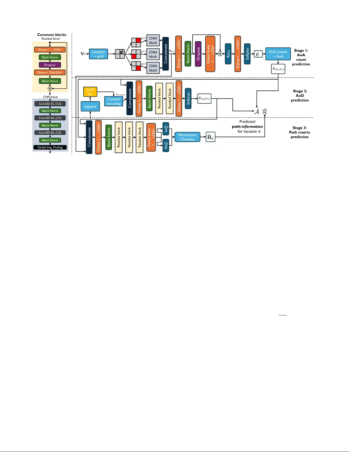
Leave a Comment