Bayesian calendar-time survival analysis with epidemic curve priors and variant-specific infection hazards

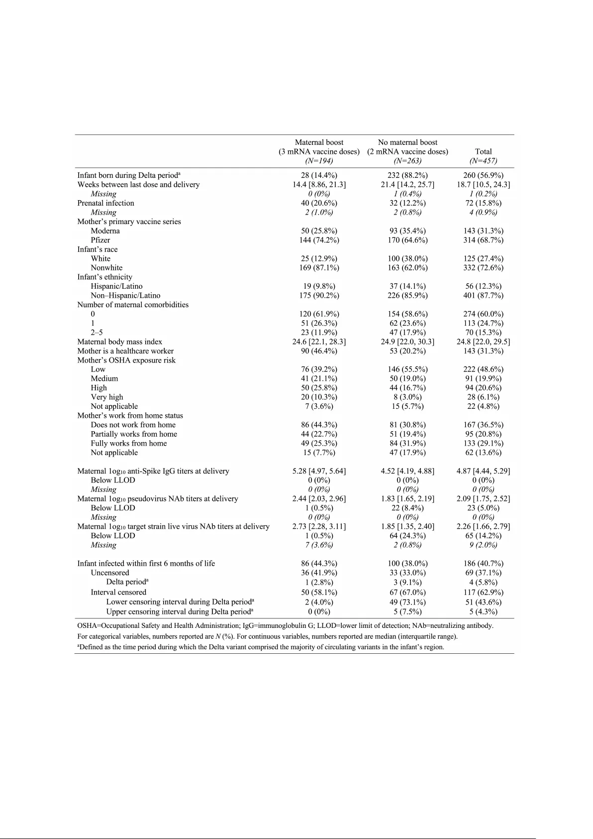
Ba y esian calendar-time surviv al analysis with epidemic curv e priors and v arian t-sp eciﬁc infection hazards Angela M Dahl 1 , 2 and Elizab eth R Bro wn 1 , 2 , 3 1 Departmen t of Biostatistics, Univ ersity of W ashington, Seattle, W ashington, U.S.A. 2 V accine and Infectious Disease Division, F red Hutc h Cancer Center, Seattle, W ashington, U.S.A. 3 Public Health Sciences Division, F red Hutch Cancer Cen ter, Seattle, W ashington, U.S.A. Abstract In this pap er, w e develop a Ba y esian calendar-time surviv al mo del moti- v ated b y infectious disease preven tion studies o ccurring during an epidemic, when the risk of infection can c hange rapidly as the epidemic curv e shifts. F or studies in whic h a biomark er is the predictor of in terest, we include the option to estimate a threshold of protection for the biomark er. If the in terven tion is h yp othesized to ha ve diﬀerent asso ciations with sev eral circulating viral v arian ts, or if the infectiousness of the dominan t v ariant(s) changes o v er the course of the study , w e treat infection from diﬀeren t v arian ts as comp eting risks. W e also in tro duce a no vel metho d for incorp orating existing epidemic curv e estimates into an informativ e prior for the baseline hazard function, en- abling estimation of the in terv ention’s association with infection risk during p eriods of calendar time with minimal follow-up in one or more comparator groups. W e demonstrate the strengths of this method via simulations, and w e apply it to data from an observ ational COVID-19 v accine study . Keyw ords Ba yesian, calendar time, epidemic curv e, infectious disease, surviv al analysis Corresp onding author Angela M Dahl adahl@fredhutch.org (507) 990-5709 1 1 In tro duction In studies of infectious disease prev en tion, assessing the asso ciation b et ween an in ter- v ention and the risk of infection is frequently complicated by temp oral (often seasonal) c hanges in the risk of exp osure to infection. This is relev an t, for example, in v accine trials for diseases suc h as inﬂuenza, coronavirus 2019 (CO VID-19), or respiratory syncy- tial virus (RSV). F or prosp ectiv e studies with time-to-even t outcomes, the estimand of in terest is often a hazard ratio obtained from a Cox prop ortional hazards mo del, which naturally incorp orates right censoring, allo ws for stratiﬁcation by site, handles p oten tial confounders via cov ariate adjustment, and allo ws for ﬂuctuations in the baseline risk of infection ov er the course of the study . 7,6,1 If a study is randomized and participan ts are enrolled quic kly , then the risk of infection is typically mo deled using a study time scale (for example, time since v accination), as randomization ensures that the av erage baseline risk of infection is approximately equal b et w een interv en tion groups at a given time on study , provided there is minimal unobserv ed heterogeneity in the risk of infection among the study p opulation. 9 Ho wev er, in nonrandomized trials, or when participants are en- rolled ov er a p erio d of time rather than all at once, it is standard to mo del infection risk in calendar time, rather than study time, to account for signiﬁcant changes in the risk of infection as the bac kground epidemic c hanges ov er calendar time, which may otherwise lead to biased comparisons. Fin tzi and F ollman 9 illustrate the imp ortance of using cal- endar time in infectious disease studies with staggered enrollmen t in order to maintain the prop ortional hazards assumption; otherwise, if time on study is used as the time scale, then the interv ention eﬀect would b e biased from the calendar time diﬀerences in the baseline hazard b et ween in terven tion groups. In the context of CO VID-19, sev eral authors ha v e highligh ted the presence of calendar time bias in observ ational COVID-19 v accine studies, 24,12 and man y studies of COVID-19 v accine eﬀectiveness and durability ha ve used calendar time in their mo dels for infection risk, either as the time scale for a Co x prop ortional hazards mo del 21,16 or as a co v ariate in a logistic or Poisson regression mo del. 36,25 In a simulated observ ational CO VID-19 v accine study closely resembling the 2021 pandemic in Denmark, Lund et al 30 found that Cox regression with a calendar time scale yielded the least biased results. While the standard Cox proportional hazards model is easily applied to infectious disease studies by using a calendar time scale, issues can still arise from its treatment of the baseline hazard function as a n uisance parameter. 6 On the one hand, the partial lik eliho o d approach implicitly allo ws for a completely ﬂexible baseline hazard function, whic h can handle the rapidly changing infection risk during an epidemic. How ever, with a ﬂexible baseline hazard function comes a tradeoﬀ: if there are an y p eriods of calendar time with minimal study follo w-up in one or more comparator groups, as is common in trials with staggered enrollment, then the mo del has no information to distinguish the 2 in terven tion eﬀect from c hanges in the baseline hazard during these time p erio ds, and the estimated interv en tion eﬀect may b e biased. F or example, consider an observ ational v accine study that b egins enrolling participants in one dose group b efore another dose group. If the epidemic is at a high p oin t during the b eginning of the study but declines b y the time the second dose group b egins enrolling, then the mo del may attribute the high rate of infections at the b eginning of the study to low protection against infection in the ﬁrst dose group rather than an esp ecially high baseline hazard during that time. T o solv e this problem, we prop ose a Bay esian approac h to a calendar-time surviv al mo del, enabling us to emplo y an informativ e baseline hazard prior to pro vide the model with information ab out infection risk during time p eriods that lack suﬃcient study data. W e prop ose using publicly a v ailable data ab out the epidemic curve to create this informative prior. The method w e dev elop in this pap er addresses several issues that can arise in trials for infectious diseases that o ccur in seasonal or epidemic patterns. First, as discussed ab o ve, the hazard of infection should b e modeled in calendar time, particularly if the trial is nonrandomized or has a long enrollmen t p erio d. Second, the baseline hazard function should ha v e the ﬂexibility to change rapidly to reﬂect the b eha vior of epidemic curves. Third, w e could ideally incorp orate prior information into the mo del to inform infection risk during calendar time p erio ds lac king suﬃcien t follow-up. F ourth, for analyses in whic h a biomarker is the predictor of in terest, we w ould lik e the option to estimate a threshold of protection. Finally , the mo del should accoun t for m ultiple circulating v ariants of the pathogen if the in terv ention is h yp othesized to be asso ciated with diﬀeren t lev els of protection from each v ariant. T o address the need for a ﬂexible baseline hazard function, our metho d uses a piecewise constan t baseline hazard function, as typical parametric forms for the baseline hazard suc h as exp onen tial or W eibull cannot capture the rapidly c hanging infection risk during an epidemic. How ever, as noted ab o v e, using a ﬂexible baseline hazard function in a calendar time mo del can lead to insuﬃcien t information to identify the in terven tion eﬀect from the baseline hazard during time p eriods with little follow-up. W e address this problem with an informativ e baseline hazard prior. Our metho d utilizes existing epidemic curv e data to deriv e an informative prior for the baseline hazard function. Our motiv ation for doing so comes from the assumption that infection risk dep ends on calendar time only through the changing risk of exp osur e to the pathogen. F ollo wing this, we exp ect the epidemic curve to reﬂect study participants’ risk of exp osure on a relativ e scale; if the rate of infections in the communit y increases tenfold o ver the course of a mon th, then w e exp ect study participants’ risk of exp osure to infection to also increase appro ximately tenfold. Once exp osed, w e assume that participants’ risk of b ecoming infected no longer dep ends on the curren t size of the epidemic, but rather on characteristics of their own immune systems and the infectiousness of the v ariant to 3 whic h they w ere exp osed. These assumptions highlight the framew ork in whic h we think of the infection pro cess: similar to the approach taken b y Halloran et al, 22 w e conceive of any infection as resulting from 1) exp osure to infection, and 2) infection once exp osed (i.e., acquisition). Tsiatis and Da vidian 42 used a similar framew ork for conceptualizing v accine eﬃcacy during the COVID-19 pandemic. Assuming the probability of infection given no exp osure is zero and the probability of exp osure is indep enden t of whether someone has b een infected previously or not, we can (informally) decomp ose the hazard of infection as Pr(infection at time t | no infection b efore time t ) = Pr(infection at time t | exp osure at time t , no infection b efore time t ) × Pr(exp osure at time t ) . In our metho d, w e mo del the probability of exp osure as a piecewise constan t function that dep ends on calendar time, and we mo del the hazard of acquisition using a standard prop ortional hazards mo del 7 with time-v arying co v ariates. The epidemic curv e will then serv e as an informative prior for the probability of exp osure. W e cannot directly use the epidemic curve itself as a prior, as the rate of infections p er p erson in the epidemic curv e data is unlikely to b e on the same scale as in our study . Instead, we use the shap e of the epidemic curv e to deriv e the shap e of the prior for the baseline hazard function while allowing the sc ale of the baseline hazard function to b e driven b y the rate of infections in our study . W e accomplish this b y choosing some reference p oin t in time to whic h w e anc hor the scale of the baseline hazard, and then w e put informativ e priors only on the r elative baseline hazard at other calendar times compared to the reference time. Man y studies of infectious diseases are interested in the association b et ween a biomark er, suc h as v accine-elicited antibo dies, and the risk of infection; how ev er, man y biomarker assa ys ha v e a lo wer limit of detection (LLOD) b elo w which w e cannot obtain a reliable measuremen t. 45 Additionally , we are often interested in estimating a threshold of protec- tion, which can guide dosage recommendations for v accines or mono clonal antibo dies. 26 If the predictor of in terest is a biomarker with a LLOD, we include a binary indicator in the hazard function denoting whether the biomark er is ab o ve or b elo w the LLOD. This allo ws estimation of the con tinuous asso ciation b et ween biomarker levels and infection risk only among biomark ers ab o v e the LLOD. If the goal is to estimate a threshold of protection, we replace this binary LLOD indicator with an indicator denoting whether the biomarker is ab o v e the threshold, and w e estimate this threshold as an additional parameter in the mo del. In b oth approac hes, the mo del assumes a constant risk of infec- tion b elo w the LLOD or threshold of protection at a given calendar time, conditional on an y time-v arying cov ariates. 4 When necessary , we treat m ultiple v ariants of the pathogen as competing risks. 35 This is relev ant in studies where multiple v arian ts are circulating that change in prev alence o ver time and ha v e diﬀeren t lev els of infectiousness, causing the risk of infection to c hange o ver calendar time giv en the same level of exp osure; as Tsiatis and Davidian 42 note, the rapidly mutating sev ere acute respiratory syndrome coronavirus 2 (SARS-CoV-2) v ariants pro vide a w ell-kno wn recent example of this. 41,2 In addition, this allows us to estimate the asso ciation b et ween the predictor of interest and infection risk separately for each v ariant, which is relev ant for man y viruses that m utate quickly , suc h as SARS-CoV- 2, 46,8 inﬂuenza, 4 and RSV 27 ; v accines for suc h viruses are typically developed to elicit an tib o dies against a sp eciﬁc v ariant, and they may be less eﬀective against other v ariants that are less similar to the targeted v ariant. This approach for estimating v arian t-sp eciﬁc v accine protection via comp eting risks is a form of siev e analysis. 18,17 The rest of this pap er is organized as follows. In Section 2, we deriv e the likelihoo d for our mo del, and w e describ e our metho d for incorp orating epidemic curv e data in to an informative prior for the baseline hazard function. In Section 3, w e demonstrate our metho d through sim ulations, including a demonstration of the bias correction that results from using an informativ e baseline hazard prior in trials with staggered enrollment. In Section 4, w e apply our metho d to the MOMI-V ax study , an observ ational study of SARS- CoV-2 v accination in pregnant women. Finally , in Section 5, we summarize the b eneﬁts and dra wbacks of our metho d, and w e discuss the results of our MOMI-V ax analysis. 2 Metho ds In this section, w e deriv e the lik eliho o d for our mo del, which incorp orates the predictor of in terest and an y baseline or time-v arying co v ariates via a proportional hazards mo del. T o enable estimation of v ariant-speciﬁc associations b et ween the predictor of in terest and the risk of infection, and to allow for changes in the pathogen’s infectiousness ov er calendar time due to new v arian ts, we form ulate our surviv al mo del as a comp eting risks mo del by deﬁning cause-sp eciﬁc hazards for each v ariant. 35 As introduced in Section 1, w e express the v arian t-sp eciﬁc hazard of infection as the pro duct of the hazard of infection given exp osur e to that v arian t, whic h w e call the hazard of acquisition, and the probabilit y of exposure to that v ariant. W e then derive the forms for the hazard of acquisition, whic h is a standard prop ortional hazards mo del, and the probability of exp osure, which is a piecewise constant function that dep ends on calendar time. Finally , we describ e a new metho d for creating an informativ e prior for the baseline hazard function b y using epidemic curv e data to inform the baseline probabilit y of exp osure as it changes o ver calendar time. Let V b e the total n umber of v ariants of interest that can infect participants in the study (for man y studies, V = 1), and let θ denote the set of mo del parameters. F or 5 participan t i , let t i 0 denote the calendar time at whic h their study follo w-up b egins. A t calendar time t , let h ( v ) A,i ( t | θ ) denote the hazard of acquisition for v arian t v , and let p ( v ) E ,i ( t | θ ) denote the probabilit y of exp osure to v ariant v . Then the cause-sp eciﬁc hazard of infection from v ariant v can b e written as h ( v ) i ( t | θ ) = h ( v ) T ,i ( t | θ ) × p ( v ) E ,i ( t | θ ) , and the ov erall hazard of infection (from any v arian t) is h i ( t | θ ) = P V v =1 h ( v ) i ( t | θ ). In the subsections that follow, we describ e the mo dels for the hazard of transmission and the probability of exp osure, whic h com bine to get the hazard of infection. 2.1 Hazard of acquisition W e mo del the hazard of acquisition (that is, the hazard of infection giv en exp osure) as a function of calendar time t dep ending on each participan t’s (p ossibly time-v arying) pre- dictor of interest X i ( t ) and susceptibility cov ariates Z A,i ( t ). W e assume that, conditional on the predictor of interest and the susceptibilit y co v ariates, the hazard of acquisition is constan t ov er time for a giv en v ariant. W e emplo y a prop ortional hazards mo del, assum- ing the co v ariates ha ve the same association with all v ariants but allo wing the predictor of in terest to hav e v arian t-sp eciﬁc asso ciations with the hazard of acquisition. W e include a parameter α ( v ) to capture the relativ e infectiousness of v ariant v compared to some reference v ariant v = 1, with α (1) = 0. Then the v ariant-speciﬁc hazard of acquisition for v ariant v at calendar time t is h ( v ) A,i ( u | θ ) = h A, 0 exp n α ( v ) + γ ( v ) X i ( t ) + Z A,i ( t ) β A o , (1) where h A, 0 is the constan t baseline hazard of acquisition. If the predictor of in terest is a biomarker, w e can optionally incorp orate a LLOD or threshold of protection X T in to the v arian t-sp eciﬁc hazard of acquisition as follows, assuming a constant risk of infection b elow X T at a given calendar time (conditional on an y cov ariates): h ( v ) A,i ( u | θ ) = h A, 0 exp n α ( v ) + γ ( v ) X i ( t ) 1 { X i ( t ) > X T } + γ ( v ) T 1 { X i ( t ) > X T } + Z A,i ( t ) β A o , (2) The threshold X T ma y b e treated as a parameter itself, allo wing estimation of a threshold of protection. 2.2 Probabilit y of exp osure W e model the probabilit y of exp osure as a function of calendar time t dep ending on some (p ossibly time-v arying) exp osure cov ariates Z E ,i ( t ). F or a participant at site s i , the probabilit y of exp osure to v ariant v dep ends on their instan taneous rate of contacts c i ( t ) and the probability a con tact at that site is infectious with that v arian t p ( v ) c,s i ( t ). 22 W e as- 6 sume that, conditional on the exp osure co v ariates, participan ts mix randomly with their comm unity at a constan t rate o ver time, so the con tact rate is c i ( t ) = c 0 exp  Z E ,i ( t ) β E  , where c 0 is the baseline contact rate. W e assume that the probabilit y a contact is infec- tious with a particular v ariant depends on calendar time due to the changing bac kground rate of infections in the comm unit y as well as the changing prev alence of that v arian t in the comm unity . W e mak e use of existing v arian t surv eillance data and treat the relative prop ortions of each v ariant in circulation as known piecewise constant functions, denoted π ( v ) s i ( t ) for v arian t v , with P V v =1 π ( v ) s i ( t ) = 1 for all t . Then the probability a con tact at site s i is infectious with v ariant v is p ( v ) c,s i ( t ) = π ( v ) s i ( t ) p c, 0 ,s i ( t ). W e appro ximate the probabilit y that a con tact at site s i is infectious with any v arian t using a piecewise constan t function, denoted p c, 0 ,s i ( t ), o ver K equally-sized in terv als of calendar time ( t 0 , t 1 ] , . . . , ( t K − 1 , t K ]. Then the probability of exposure to infection from v ariant v is the pro duct of their contact rate and the probabilit y a contact is infectious with v ariant v : p ( v ) E ,i ( t | θ ) = c i ( t ) p ( v ) c,s i ( t ) = c 0 π ( v ) s i ( t ) p c, 0 ,s i ( t ) exp  Z E ,i ( t ) β E  . (3) 2.3 Hazard of infection T aking the pro duct of our expressions for the hazard of acquisition h ( v ) A,i ( t | θ ) and the probabilit y of exp osure p ( v ) E ,i ( t | θ ) for each v arian t, the v ariant-speciﬁc hazard of infection for v ariant v is h ( v ) i ( t | θ ) = h A, 0 exp n α ( v ) + γ ( v ) X i ( t ) + Z A,i ( t ) β A o × c 0 π ( v ) s i ( t ) p c, 0 ,s i ( t ) exp  Z E ,i ( t ) β E  . (4) If the mo del includes a LLOD or threshold for the predictor of interest, then the v ariant- sp eciﬁc hazard of infection is h ( v ) i ( t | θ ) = h A, 0 exp n α ( v ) + γ ( v ) X i ( t ) 1 { X i ( t ) > X T } + γ ( v ) T 1 { X i ( t ) > X T } + Z A,i ( t ) β A o × c 0 π ( v ) s i ( t ) p c, 0 ,s i ( t ) exp  Z E ,i ( t ) β E  , (5) Because we only observ e infections, but not exp osures and acquisition ev ents separately , the parameters β A , β E , h A, 0 , c 0 , and p c, 0 ,s i ( t ) are not identiﬁable on their own. Instead, w e com bine them into a single vector of co eﬃcien ts β and a single piecewise constan t baseline hazard term h ( v ) 0 ,s i ( t ) = h A, 0 c 0 p c, 0 ,s i ( t ). Keep in mind that the baseline hazard dep ends on calendar time only through p c, 0 ,s i ( t ), the probability a con tact at site s i is infectious. W e also cannot typically rule out unmeasured confounding in the relationship b et w een the predictor of in terest and the risk of infection, unless the study is randomized; therefore, γ ( v ) and γ ( v ) T actually estimate the asso ciation b etw een the predictor of interest and the threshold of protection (if applicable) and the hazard of infection ov erall, not on 7 the hazard of acquisition. Then the ﬁnal form of the v ariant-speciﬁc hazard of infection is h ( v ) i ( t | θ ) = π ( v ) s i ( t ) h ( v ) 0 ,s i ( t ) exp n α ( v ) + γ ( v ) X i ( t ) + Z i ( t ) β o . (6) If the model includes a LLOD or threshold of protection for the predictor of interest, then the ﬁnal form of the v ariant-speciﬁc hazard of infection is h ( v ) i ( t | θ ) = π ( v ) s i ( t ) h ( v ) 0 ,s i ( t ) exp n α ( v ) + γ ( v ) X i ( t ) 1 { X i ( t ) > X T } + γ ( v ) T 1 { X i ( t ) > X T } + Z i ( t ) β o . (7) 2.4 Lik eliho o d F ollowing Prentice et al, 35 w e express the lik eliho o d in terms of the v ariant-speciﬁc hazard functions. F or uncensored or right censored participan ts, let T i denote their surviv al time and ∆ i indicate right censoring. F or in terv al censored participants, let ( L i , R i ) denote their censoring in terv al. In Section 2.3, w e deﬁned the v ariant-speciﬁc hazard function h ( v ) i ( t | θ ). Now, assuming it is only p ossible to b e infected with one v ariant at a time, the o verall hazard function is deﬁned as the sum of the v ariant-speciﬁc hazard functions h i ( t | θ ) = V X v =1 h ( v ) i ( t | θ ) , (8) and the o verall survivor function is deﬁned as S i ( t | θ ) = exp n − Z t t i 0 h i ( u | θ ) du o = exp n − Z t t i 0 V X v =1 h ( v ) i ( u | θ ) du o . (9) 2.4.1 Kno wn infecting v arian ts F or uncensored or right censored participants with infecting v ariant v i ( v i is arbitrary for righ t censored participan ts), the likelihoo d con tribution for their surviv al time T i , righ t censoring indicator ∆ i , and infecting v ariant v i L ( T i , ∆ i | θ , v i ) = h h ( v i ) i ( T i | θ ) i ∆ i × S i ( T i | θ ) . (10) F or in terv al censored participants, the likelihoo d contribution for their censoring in terv al ( L i , R i ) and infecting v ariant v i is L ( L i , R i | θ , v i ) = Z R i L i h h ( v i ) i ( t | θ ) × S i ( t | θ ) i dt. (11) 8 2.4.2 Unkno wn infecting v arian ts If the infecting v ariants are unkno wn, the lik eliho o d for eac h observed infection uses the o verall hazard function instead of the v ariant-speciﬁc hazard function. F or uncensored or righ t censored participants, the lik eliho o d contribution for their surviv al time T i and righ t censoring indicator ∆ i is L ( T i , ∆ i | θ ) = h h i ( T i | θ ) i ∆ i × S i ( T i | θ ) . (12) F or in terv al censored participants, the likelihoo d contribution for their censoring in terv al ( L i , R i ) is L ( L i , R i | θ ) = Z R i L i h h i ( t | θ ) × S i ( t | θ ) i dt = S i ( L i | θ ) − S i ( R i | θ ) . (13) 2.5 Informativ e baseline hazard prior based on an epidemic curv e W e now derive an informative prior for the baseline hazard function that utilizes existing epidemic curv e estimates. An informative prior adds information to the mo del ab out infection risk during calendar times with little follo w-up, improving identiﬁabilit y of γ and β . Our motiv ation for using epidemic curve data comes from our form ulation of the hazard function, in which w e isolated the probabilit y a contact is infectious as the only parameter in the hazard function that dep ends on calendar time. The probability a con tact is infectious constitutes a portion of the baseline hazard function that comes from the probabilit y of exposure. As long as the epidemic curv e w ell represen ts the bac kground rate of infections in the communit y with which study participan ts are mixing, it should b e appro ximately prop ortional to the probability a study participant’s contact is infectious o ver calendar time, though it will not necessarily b e on the same scale. Lev eraging this assumption, we use the epidemic curve as an informativ e prior for the shap e of the baseline hazard function while using a weakly informative prior for its sc ale . W e assume throughout that the epidemic curve corresp onds to the ov erall num b er of infections and is not separated b y v ariant. Recall that the baseline hazard of infection at study site s i is a piecewise constan t function ov er K equally-sized interv als of calendar time ( t 0 , t 1 ] , . . . , ( t K − 1 , t K ], and it is made up of three terms: the baseline hazard of acquisition h A, 0 , the baseline con tact rate c 0 , and the probability a contact is infectious with p c, 0 ,s i ( t ). Because these terms are not iden tiﬁable on their own, w e combine them into a single baseline hazard term h 0 ,s i ( t ). In order to more readily put a prior on the shap e of the baseline hazard function, we now reparameterize it as h 0 ,s i ( t ) = h ref ,s i × r s i ( t ), where h ref ,s i is the baseline hazard during some reference in terv al of time and r s i ( t ) is the relative baseline hazard at calendar time 9 t compared to the reference interv al. The relative baseline hazard is a piecewise constant function taking the v alues r 1 ,s i , . . . , r K,s i during time interv als ( t 0 , t 1 ] , . . . , ( t K − 1 , t K ]. The relativ e baseline hazard during the reference interv al is constan t at r ref ,s i = 1. In this reparameterization of the baseline hazard function, the relative baseline haz- ard is in fact equal to the relativ e probabilit y a contact is infectious at calendar time t compared to the reference interv al: r s i ( t ) = p c, 0 ,s i ( t ) /p c, 0 ,s i ( t ref ). This allo ws us to use the epidemic curve as an informativ e prior for the relative baseline hazard parameters r 1 ,s i , . . . , r K,s i . F or site s i , we sp ecify independent priors log( r k,s i ) ∼ N ( µ k,s i , σ 2 k,s i ) for k = 1 , . . . , K , where µ k,s i is the epidemic curve’s estimated log relative n umber of infec- tions during in terv al k compared to the reference interv al, and σ 2 k,s i is derived from the conﬁdence interv als that t ypically accompany epidemic curve data and ma y b e scaled up to mak e the prior less informative. F or the reference in terv al, we recommend c ho osing the time in terv al with the most ob- serv ed infections in the study in order to maximize the amoun t of information ab out h ref ,s i . W e put a weakly informativ e prior on the baseline hazard during the reference interv al so that the scale of the p osterior baseline hazard function is driv en by the observed rate of infections in the study . F or site s i , we sp ecify the prior log ( h ref ,s i ) ∼ N ( µ ref ,s i , σ 2 ref ,s i ), where µ ref ,s i is the estimated log rate of infections p er p erson-time during the reference in terv al, and σ ref ,s i is derived from the epidemic curve’s conﬁdence interv als and ma y scaled up to mak e the prior less informative. 2.6 Prior elicitation F or the baseline hazard at each study site s i , we use a weakly informativ e prior for h ref ,s i and informative priors for the relativ e baseline hazard parameters r 1 ,s i , . . . , r K,s i , as describ ed in Section 2.5. F or the relative infectiousness parameters α ( v ) for eac h v ariant (if relev ant), we recommend using existing data on circulating v arian ts to form an informative prior in the form of α ( v ) ∼ N  µ ( v ) α , ( σ ( v ) α ) 2  , where µ ( v ) α is the estimated log relativ e infectiousness of v arian t v compared to v arian t 1 and σ ( v ) α is the corresp onding estimated SD. If estimating a threshold of protection X T for the predictor of in terest, w e recommend a uniform prior X T ∼ Uniform[ X ℓ , X u ], where X ℓ and X u are c hosen sensibly based on the observed range of v alues of the predictor of interest X . F or the remaining parameters, w e follo w the recommendations of the Stan developers 14 and use w eakly informativ e priors that are scaled to reﬂect the expected order of magnitude of the parameter, so that the prior do es not place most of its mass on unrealistically extreme parameter v alues. 15,13 F or real-v alued co eﬃcient parameters, we use N (0 , 2) priors if we exp ect its absolute v alue to b e ab o v e 0.1 or N (0 , 0 . 5) priors if we expect its absolute v alue to b e below 0.1 (this is relev an t in our application to the MOMI-V ax study in Section 4, which includes sev eral co eﬃcien ts on the n um b er of days b efore or after birth, 10 whic h we exp ect to b e v ery small). F or multiv ariate co eﬃcien t parameters, such as β , w e use indep endent N (0 , 2) or N (0 , 0 . 5) priors as describ ed ab ov e for each elemen t in the parameter v ector. 2.7 Implemen tation F or the simulations and data application in this pap er, the p osterior distributions w ere estimated using Stan 39 via the interface RStan 38 in R. 37 When necessary , in tegration of the Normal PDF in the likelihoo d is appro ximated using Stan’s normal lcdf function. 40 Stan co de for ﬁtting this mo del is av ailable in the Supp orting Information. 3 Sim ulations W e applied our metho d to simulated CO VID-19 v accine trials with v arying sample sizes and study designs. F or each sample size ( N = 100, 500, 1,000, or 5,000), we sim ulated 50 CO VID-19 v accine trials with participan ts randomized 1:1 to either an active or placeb o group. Enrollmen t dates w ere randomly sampled b et ween July 1 , 2021–December 1, 2021 for the v accine group and b et ween Marc h 1–Septem b er 1, 2021 for the placeb o group, so the v accine group had an o verall higher baseline hazard compared to the placeb o group. P articipants w ere randomly assigned to a site in the United States (US) state of Georgia, New Y ork, or W ashington, and were follow ed with visits ev ery tw o months for up to six mon ths or until they b ecame infected. 3.1 Sim ulation metho ds F or each participant i , we denoted their randomized interv ention group X i , and w e gen- erated an additional baseline co v ariate Z i iid ∼ Bernoulli(0 . 5). W e simulated infection times using the hazard function h i ( t ) = h ref ,s i r s i ( t ) exp n γ X i + β Z i o . (14) T o simplify our simulations, w e set the num b er of circulating v arian ts to 1. W e randomly c hose 20% of infections to b e in terv al censored, with lo wer and upp er censoring dates set to the visit dates (at Mon ths 0, 2, 4, or 6) b efore and after their true infection times. T rue parameter v alues were set to γ = − 1 and β = − 0 . 5. The baseline hazard function for eac h site w as generated using the US state–lev el SARS-CoV-2 epidemic curve estimates from the Institute for Health Metrics and Ev aluation (IHME). 23 F or eac h simulated dataset, w e ﬁt our calendar-time surviv al mo del using one of the follo wing priors for the relative baseline hazard parameters { r k,s i } K k =1 and the baseline 11 hazard during the reference interv al h ref ,s i at each site. Figure S1 displays these prior distributions. 1. Correctly sp eciﬁed baseline hazard prior: The priors w ere formed using the IHME’s SARS-CoV-2 epidemic curv e data 23 follo wing the metho d describ ed in Section 2.5. F or time in terv al ( t k − 1 , t k ] and site s i , the prior for the relativ e baseline hazard w as log ( r k,s i ) ∼ N ( µ k,s i , σ 2 k,s i ), where the SD σ k,s i w as set to 0.25 (informativ e), 1 (mo derately informativ e), 2.5 (w eakly informativ e), or 5 (uninformativ e). F or ev ery site, the prior for the baseline hazard during the reference interv al was log( h ref ,s i ) ∼ N ( µ ref ,s i , 5 2 ). 2. Missp eciﬁed baseline hazard prior: The priors were formed using the IHME’s SARS- CoV-2 epidemic curv e data 23 from incorrect states (P ennsylv ania, Missouri, or Ohio), 30 days prior. F or a giv en time in terv al and site, the prior for the rel- ativ e baseline hazard was log( r k,s i ) ∼ N ( µ k,s i , σ 2 k,s i ), where the SD σ k,s i w as set to 0.25, 1, 2.5, or 5. F or every site, the prior for the baseline hazard during the reference in terv al was log( h ref ,s i ) ∼ N ( µ ref ,s i , 5 2 ). 3. Flat baseline hazard prior: F or a giv en time in terv al and site, the prior for the relativ e baseline hazard w as log( r k,s i ) ∼ N ( µ k,s i , σ 2 k,s i ), where the SD σ k,s i w as set to 2.5 or 5. F or ev ery site, the prior for the baseline hazard during the reference in terv al was log( h ref ,s i ) ∼ N ( − 5 , 5 2 ). W e put N (0 , 2) priors on γ and β . 3.2 Sim ulation results Figure 1 shows the distribution of p osterior means and the co verage of the 95% p osterior credible in terv als (CrIs) for γ , the parameter of in terest, which determines the asso cia- tion b etw een interv en tion group and the hazard of infection. T able S1 in the Supp orting Information displays the full results for b oth γ and β , whic h determines the asso ciation b et w een the cov ariate Z i and the hazard of infection. When a correctly sp eciﬁed infor- mativ e baseline hazard prior ( σ 2 k,s i = 0 . 25) w as used, then the p osterior mean of γ was un biased and the 95% CrI cov erage w as excellen t, and correctly sp eciﬁed but less infor- mativ e priors ( σ 2 k,s i = 1 , 2 . 5 , or 5) also resulted in less biased estimates and impro ved co verage compared to the ﬂat prior. How ev er, if an a missp eciﬁed baseline hazard prior w as used, then the p osterior mean of γ was more biased as it b ecame more informativ e. The ﬂat, uninformativ e prior (with σ 2 k,s i = 5) was only unbiased and had cov erage ab out 95% at a v ery large sample size ( N = 5000); in smaller sample sizes, the ﬂat prior re- sulted in signiﬁcan t bias. F or β , the cov erage and bias w ere less sensitiv e to a missp eciﬁed informativ e baseline hazard prior. 12 4 Application to the MOMI-V ax study W e now demonstrate the metho d in tro duced in this pap er by applying it to data from the MOMI-V ax study , a multisite, prospective, longitudinal cohort study of mother-infan t pairs following maternal COVID-19 v accination during pregnancy . The primary aim of the study was to determine the asso ciation b et w een sev eral biomarkers (including anti– full-length spike [Spike] imm unoglobulin G [IgG], pseudovirus neutralizing antibo dies [NAbs] against the target v accine strain, and live virus NAbs against sev eral v ariants) in the infant and the infan t’s risk of SARS-CoV-2 infection within the ﬁrst six mon ths of life. In addition, the study aimed to compare infants whose mothers either received a complete series (2 doses) of a monov alent messenger RNA (mRNA) COVID-19 v accine during pregnancy (the “nonbo osted” group) or who received a b o oster dose (3rd dose) during pregnancy (the “b o osted” group). 33 Cardemil et al 5 found that infan ts of mothers who had received a b o oster dose during pregnancy had signiﬁcan tly higher an ti-Spik e IgG titers, pseudo virus NAb titers, and live virus NAb titers at delivery and w ere 56% less likely to b e infected with SARS-Co v-2 during the ﬁrst six months of life compared to infants of nonbo osted mothers. When the SARS-CoV-2 case deﬁnition w as expanded to include interv al censored infections (iden- tiﬁed through sero conv ersion of N protein b etw een study visits), infants whose mothers had received a b o oster dose were 75% less likely to b e infected. These estimates were ob- tained using calendar time Co x prop ortional hazards mo dels stratiﬁed by site, p erformed on a subset of the data from calendar times with suﬃcient follow-up in each dose group in order to ensure reliable inference. As noted by Cardemil et al, 5 analysis of the MOMI-V ax data w as complicated due to the timing of bo oster a v ailability: the ma jorit y of the t w o-dose group of infan ts w ere b orn b efore the Omicron wa ve, while the ma jority of the three-dose group were b orn during the Omicron wa v e, leading to several mon ths at the b eginning and end of the study when only a single group w as b eing follow ed. They addressed this problem by limiting the data to only p erio ds of calendar time with > 0.8 p erson-y ears of follo w-up in b oth dose groups and in all infant age groups (0–2 mon ths and 2–6 months). The metho d in tro duced in this pap er enables estimation of the asso ciation b etw een antibo dy lev els at delivery and infection risk during the ful l study p erio d by using an informative prior for the baseline hazard of infection, allowing the mo del to b orrow information from the prior during time p erio ds with little or no data from a comparator group. Because w e now retain data from the full study p erio d, we now hav e many infections from the Delta p erio d that the Cardemil et al analysis did not include. Our metho d allo ws us to estimate the asso ciation b et w een an tib o dies and the risk of Delta or Omicron infection separately . Because the MOMI-V ax study did not collect information on whic h v arian t caused each infection, we use v ariant surv eillance data from the US Centers for Disease Con trol and Preven tion 13 (CDC) 43 to deﬁne the relative prop ortions of Delta and Omicron v arian ts in circulation o ver time at each study site. W e now apply our metho d to estimate the asso ciation b etw een sev eral antibo dies in the mother at delivery and the infant’s risk of SARS-CoV-2 infection during the ﬁrst six mon ths of life. It is standard practice to collect blo o d from mothers when they are admitted for deliv ery , 31 and maternal blo o d is typically easier and more reliable to collect than infan ts’ cord blo o d. 3 In addition, m ultiple studies, 29 including a preliminary analysis of the MOMI-V ax data, 32 ha ve shown that maternal SARS-CoV-2 antibo dies (from b oth infection and v accination) are transferred to the infant via the placenta, making them an ideal biomark er for assessing infants’ protection against SARS-CoV-2 infection. Because a substantial prop ortion of mothers had antibo dy titers that had w aned to b elo w the LLOD by delivery , our mo del includes an asso ciation b etw een antibo dy levels at deliv ery and infection risk only for antibo dy lev els ab o v e the LLOD. F or maternal an tib o dies b elo w the LLOD at deliv ery , we assume the hazard of infection is equal to that of mothers who ha ve no an tib o dies at delivery , conditional on the cov ariates included in Z i ( t ). W e also ﬁt a second mo del in which w e estimate the maternal an tib o dy threshold b elo w whic h infants’ hazard of infection is equal to that of mothers with no antibo dies. This second analysis gives insigh t in to the minimum lev el at whic h maternal antibo dies protect infan ts against SARS-CoV-2 infection. 4.1 MOMI-V ax analysis metho ds W e assessed the relationship b et w een three antibo dies in the mothers at deliv ery and their infants’ risk of SARS-CoV-2 infection: an ti-Spik e IgG, pseudovirus NAbs against the ancestral W uhan strain (614BD (expressed as the concentration required to inhibit 50% of viral en try and replication [IC50]), and live virus NAbs to the target v accine strain (D614G) (expressed as the inhibitory dilution required to achiev e 50% neutralization [ID50]). F or brevity , w e refer to these an tib o dies as anti-Spik e IgG, pseudo virus NAbs, and target strain liv e virus NAbs. F or eac h antibo dy of in terest, w e p erformed t wo analyses: ﬁrst, an analysis using the LLOD as the threshold b eneath which the an tib o dies hav e no asso ciation with the hazard of infection, and second, an analysis in which we estimate this threshold as a parameter itself. The outcome was deﬁned as SARS-CoV-2 infection iden tiﬁed either through veriﬁed maternal rep ort (conﬁrmed by laboratory testing) or through sero con v ersion of N protein b et w een study visits. The hazard functions for each mo del are shown b elow. The sup erscripts ( d ) and ( o ) denote the Delta and Omicron v ariant, resp ectively; X i is the mother’s log 10 an tib o dy lev el at deliv ery , X ( ℓ ) is the log 10 LLOD for the antibo dy of interest; X T is the estimated log 10 an tib o dy threshold (for the estimated threshold analysis); and Z i is a v ector of baseline cov ariates. T o match the Cardemil et al analysis, 5 Z i includes the follo wing 14 baseline cov ariates: the mother’s primary CO VID-19 v accine series type (Moderna or Pﬁzer), race, ethnicity , the num b er of maternal comorbidities, maternal b o dy mass index (BMI), the mother being a healthcare w orker, the mother’s Occupational Safet y and Health Administration (OSHA) exp osure risk, and the mother’s w ork from home status. Data for π ( d ) s i ( t ) and π ( o ) s i ( t ) came from the CDC’s SARS-CoV-2 v arian t surv eillance data. 43 The infecting v arian ts w ere not collected in the MOMI-V ax study , so when ﬁtting the mo del, we use the form of the lik eliho o d for unkno wn infecting v ariants presented in Section 2.4.2. The hazard function for the LLOD threshold analysis is h i ( t ) = π ( d ) s i ( t ) h ref ,s i r s i ( t ) exp n γ ( d ) X i 1 { X i > X ( ℓ ) } + γ ( d ) ( ℓ ) 1 { X i > X ( ℓ ) } + Z i β h o + π ( o ) s i ( t ) h ref ,s i r s i ( t ) exp n α ( o ) + γ ( o ) X i 1 { X i > X ( ℓ ) } + γ ( o ) ( ℓ ) 1 { X i > X ( ℓ ) } + Z i β h o . (15) The hazard function for the estimated threshold analysis is h i ( t ) = π ( d ) s i ( t ) h ref ,s i r s i ( t ) exp n γ ( d ) X i 1 { X i > X T } + γ ( d ) T 1 { X i > X T } + Z i β h o + π ( o ) s i ( t ) h ref ,s i r s i ( t ) exp n α ( o ) + γ ( o ) X i 1 { X i > X T } + γ ( o ) T 1 { X i > X T } + Z i β h o . (16) F or the estimated threshold analysis, X T is given the prior X T ∼ Unif( X ( ℓ ) , X 1 / 2 ), where X 1 / 2 is the median observ ed biomarker v alue among those ab ov e the LLOD. F or eac h antibo dy and threshold analysis, we ﬁt our mo del using three diﬀerent pri- ors for the relative baseline hazard function parameters { r k,s i } K k =1 . W e used the IHME’s SARS-CoV-2 epidemic curv e estimates 23 to form the informative and mo derately infor- mativ e baseline hazard priors following the method describ ed in Section 2.5. Figure 2 sho ws the priors used in the MOMI-V ax analyses. 1. Informativ e baseline hazard prior: F or each calendar time in terv al ( t k − 1 , t k ] and site s i , log( r k,s i ) ∼ N ( µ k,s i , 0 . 25 2 ) and log( h ref ,s i ) ∼ N ( µ ref ,s i , 5 2 ). 2. Mo derately informativ e baseline hazard prior: F or each calendar time interv al ( t k − 1 , t k ] at eac h site s i , log( r k,s i ) ∼ N  µ k,s i , 1  and log( h ref ,s i ) ∼ N ( µ ref ,s i , 5 2 ). 3. Uninformativ e baseline hazard prior: F or all time in terv als ( t k − 1 , t k ] at eac h site s i , the mean of the relative baseline hazards w as set to µ k,s i , the mean relativ e baseline hazard rep orted by the IHME in that site ov er all time in terv als, and the SDs w ere all set to 2.5. The resulting priors were log ( r k,s i ) ∼ N ( µ k,s i , 5 2 ) and log( h ref ,s i ) ∼ N ( µ ref ,s i , 5 2 ). F or α ( o ) , w e used the informative prior α ( o ) ∼ N  log(2) , 0 . 2  based on previous research suggesting that the Omicron v ariant is appro ximately t wice as infectious as the Delta v ariant. 2 F or γ ( d ) and γ ( o ) in the estimated threshold analysis, w e used a truncated Normal 15 prior γ ( d ) , γ ( o ) iid ∼ N (0 , 2) 1 ( −∞ , 0), whic h constrains the maternal antibo dy lev els to b e asso ciated with only a reduced risk of infection compared to lev els b elo w the threshold. In the LLOD threshold analysis, w e used the prior γ ( d ) , γ ( o ) iid ∼ N (0 , 2). F or the remaining parameters γ ( d ) ( ℓ ) , γ ( o ) ( ℓ ) , γ ( d ) T , γ ( o ) T , and β , we used N (0 , 2) priors. F or each antibo dy of interest, threshold analysis, and baseline hazard prior, we ﬁt a Stan mo del with 4 chains of 4000 iterations (for the LLOD threshold analyses) or 8000 iterations (for the estimated threshold analyses), discarding the ﬁrst half of eac h c hain as burn-in. T o assess con v ergence, w e ev aluated the p osterior trace plots and ensured ˆ R w as b elo w 1.05 for all parameters. 44 T o assess mo del ﬁt, we randomly selected 100 samples from the posterior and generated predicted surviv al times for eac h infan t. Because a signiﬁcan t amount of infections w ere interv al censored b et ween Mon ths 0, 2, or 6, w e compared the predicted cumulativ e incidences to the observed cumulativ e incidences at Mon ths 2 and 6 to assess mo del ﬁt. 4.2 Results of the MOMI-V ax analysis T able 1 summarizes the baseline characteristics and SARS-CoV-2 infection outcomes among infan ts in the MOMI-V ax study . Our analysis included 457 infan ts whose mothers either receiv ed a complete series (2 doses) of a mono v alent messenger RNA (mRNA) CO VID-19 v accine during pregnancy or who received a b o oster dose (3rd dose) during pregnancy , whose mothers had at least one antibo dy measurement a v ailable at delivery , and who had complete data for all of the baseline co v ariates in our mo del. Of these infan ts, 263 w ere b orn to nonbo osted (2 dose) mothers and 194 w ere b orn to b o osted (3 dose) mothers. The nonbo osted group was b orn betw een July 2021 and June 2022 (median Octob er 2021), while the b o osted group w as b orn b etw een October 2021 and August 2022 (median F ebruary 2022). During the ﬁrst 6 mon ths of life, 100 infan ts (38%) of nonbo osted mothers w ere infected with SARS-CoV-2, and 86 infants (44%) of b o osted mothers w ere infected with SARS-CoV-2. Only 4 uncensored infections o ccurred during the Delta p erio d (b efore mid-to-late December 2021, dep ending on the state, when the ma jority of circulating v ariants were Delta), and 51 interv al censored infections might ha ve o ccurred as early as the Delta p erio d, most of whic h also spanned the Omicron p erio d. F or all an tib o dies considered in this analysis, bo osted mothers had higher median titers at deliv ery than nonbo osted mothers (Figure 3). All anti-Spik e IgG measurements w ere in the detectable range (ab o v e the LLOD) at delivery , while 22 nonbo osted mothers and 1 b o osted mother had undetectable pseudovirus NAb measuremen ts at delivery , and 64 non b o osted mothers and 1 b o osted mother had undetectable live virus NAb measuremen ts at delivery . T able 2 displays the p osterior means and 95% CrIs for the parameters of interest related to the asso ciation b etw een maternal antibo dies and the risk of SARS-CoV-2 16 infection from either the Delta or Omicron v ariant, as w ell as the estimated threshold at whic h maternal an tib o dies are asso ciated with infants’ infection risk. Figure 4 summarizes the p osterior distributions for this threshold. The mo del was unable to iden tify an anti- Spik e IgG threshold. Because so few infan ts were infected during the Delta p erio d, most of whom w ere in the non b o osted group, the estimates for the Delta p erio d are unreliable; therefore, only the Omicron results are included in the ﬁgures in this paper. T ables and ﬁgures con taining the results for the Delta p erio d are av ailable in the Supp orting Information (see Figures S2 and S3). All analyses found that higher maternal an tib o dy titers w ere asso ciated with a re- duced risk of SARS-CoV-2 infection with the Omicron v ariant; ho w ever, the informative baseline hazard prior attenuated the association to w ard less risk reduction, suggesting that mo del with the uninformativ e baseline hazard prior o verestimates the asso ciation b et w een maternal an tib o dies and reduced risk of infection. T o aid in interpreting the results, Figure 5 sho ws the p osterior relative risk reduction for SARS-CoV-2 infection in infan ts at diﬀeren t maternal an tib o dy lev els compared to either the minim um observed an tib o dy lev el in the study or the estimated an tib o dy threshold. In addition, to high- ligh t the diﬀerences in risk b et ween the nonbo osted and b o osted groups b eyond calendar time and maternal an tib o dy levels, Figure 6 sho ws the p osterior relative risk reduction for SARS-CoV-2 infection in infants, comparing “a verage” b o osted infants to “av erage” non b o osted infants. The p osterior distributions for the asso ciation b etw een the baseline cov ariates and infection risk w ere similar across the analyses using diﬀerent baseline hazard priors and diﬀeren t an tib o dies (see T able S2 and Figure S5 in the Supporting Information). All Stan mo dels conv erged to a p osterior with MCMC c hains that mixed w ell with ˆ R < 1 . 05 for all parameters, and all mo dels predict cumulativ e incidence of SARS-CoV-2 infection in the infan ts v ery close to the observ ed cumulativ e incidence (see Figures S4 and S6 in the Supp orting Information). 5 Discussion W e hav e developed a Bay esian surviv al mo del in calendar time that is tailored to infec- tious disease studies o ccurring during an epidemic. W e introduced a metho d for creating an informativ e prior for the baseline hazard function, enabling the incorp oration of out- side data ab out the epidemic into our understanding of participants’ risk of exp osure to infection during the study . W e form ulated our mo del as a comp eting risks mo del, which allo ws us to estimate v ariant-speciﬁc asso ciations b et w een the predictor of in terest and the risk of infection. F or studies in whic h a biomarker is the predictor of interest, w e included the option to estimate a threshold of protection for the biomark er. Because our method has a fully sp eciﬁed lik eliho o d, it easily incorp orates in terv al censoring in 17 addition to righ t and left censoring. Our simulation results demonstrate that when calendar time bias causes the com- parator groups to hav e v ery diﬀerent baseline hazards of infection, using an informativ e prior for the shap e of the baseline hazard function corrects the bias in estimates of γ , the asso ciation betw een the predictor of in terest and the hazard of infection, that is otherwise presen t when an uninformative prior is used. How ev er, using a missp eciﬁed informative prior can induce bias in estimates of b oth γ and other co eﬃcients in the hazard func- tion, emphasizing the need for careful consideration of whether the epidemic curv e used to create the informative prior truly reﬂects the changing risk of exp osure in the study p opulation. State-lev el epidemic curve data suc h as the IHME data used in this pap er ma y not suﬃciently reﬂect the relativ e risk of exp osure in certain studies, such as studies in rural p opulations or with targeted enrollment of high-risk participan ts. When w e applied our metho d to the MOMI-V ax study , we found that higher maternal an tib o dy titers at delivery were asso ciated with reduced risk of infection in their infants during the ﬁrst six months of life. Using an informative baseline hazard prior attenuated this association to ward less protection against infection. This atten uation is unsurprising: the infants of nonbo osted mothers were largely b orn at a lo w p oint in the epidemic, so their antibo dy levels were highest when infection risk w as comparatively low, while the infan ts of b o osted mothers w ere largely b orn at higher p oints in the epidemic, during the ﬁrst or second Omicron wa ves. Without an informative baseline hazard prior, the mo del lik ely attributes the lack of early infections in the non b o osted group to an esp ecially strong antibo dy eﬀect, as non b o osted mothers’ an tib o dy lev els w ere muc h low er than b o osted mothers’. With an informative baseline hazard prior, the mo del knows that the non b o osted group had a lo wer baseline risk of infection during this time, decreasing the strength of the an tib o dies’ asso ciation with infection risk. W e also applied our metho d to the MOMI-V ax data to estimate a threshold ab ov e whic h maternal pseudovirus and target strain live virus an tib o dies are asso ciated with protection from SARS-CoV-2 infection in their infan ts. This is the ﬁrst time a threshold at whic h an tib o dies pro vide protection against SARS-CoV-2 infection has been estimated for infan ts. When w e incorp orated outside information ab out the epidemic through an informativ e baseline hazard prior, our results suggest the need for slightly higher mater- nal an tib o dy levels to pro vide their infants with protection from SARS-COV-2 infection during the ﬁrst six months of life, whic h a b o oster dose during pregnancy helps pro vide. It should b e noted that the estimated threshold should not b e in terpreted as a causal or biological cutoﬀ, but rather an approximate p oint at which antibo dies are asso ciated with protection from infection in this study p opulation and under this mo del. Because our results are from an observ ational study , more research is needed, preferably from a randomized study , to establish a threshold of protection for infants. F uture research may also consider diﬀeren t relationships b et ween the antibo dies and infection risk, suc h as a 18 logistic relationship, rather than a linear relationship with a sharp cutoﬀ at the threshold. Ideally , w e would hav e lik ed to use the metho d prop osed in this pap er to p erform a mediation analysis to quan tify how muc h infan ts’ protection against SARS-CoV-2 infec- tion is mediated through their or their mothers’ antibo dies. How ev er, the observ ational nature of the MOMI-V ax data made calculating counterfactual outcomes imp ossible: man y nonbo osted mothers received their second v accine dose during the third trimester of pregnancy , making a b o oster dose imp ossible, which violates the p ositivit y assumption required for a causal mediation analysis. 34 More researc h will b e needed to establish a causal asso ciation betw een infan t or maternal antibo dies and infan ts’ risk of SARS-CoV-2 infection. Our results are in line with previous w ork on immune correlates of protection against CO VID-19 disease in v accinated adults. While the exact estimates v ary b y study , anti- Spik e IgG titers, pseudo virus NAbs, and (if measured) live virus NAbs b een shown to reliably predict v accine-elicited protection against CO VID-19. 20,11,10,19 Along with the previously published MOMI-V ax results for infan ts’ antibo dies at birth, 5 our results sup- p ort these an tib o dies as predictors of protection against SARS-CoV-2 infection in in- fan ts. Ho wev er, w e caution that the MOMI-V ax results are not directly comparable to previously published results on correlates of protection against SARS-CoV-2 infection for sev eral reasons. First, the MOMI-V ax study w as observ ational, and the non b o osted and b o osted groups diﬀerent signiﬁcan tly in their characteristics; for example, mothers who receiv ed a b o oster dose during pregnancy were more likely to b e non white and to ha v e a higher risk of exp osure at work. There are very likely additional, unmeasured con- founders aﬀecting the asso ciation b et ween maternal antibo dies and infan ts’ infection risk in the MOMI-V ax study . Second, the MOMI-V ax study used SARS-CoV-2 infection as its outcome, rather than symptomatic CO VID-19 disease, as w as used in most CO VID-19 v accine eﬃcacy trials. Third, the study p opulation (infan ts whose mothers had receiv ed a CO VID-19 v accine) is v ery diﬀerent from the adult p opulations on whic h the previous results are based on. Finally , the MOMI-V ax study did not include any mothers who had nev er b een v accinated, unlike randomized trials that included a placeb o group. Our metho d for incorp orating epidemic curve data in to an informativ e prior for the baseline hazard of infection is applicable to a v ariet y of settings. In particular, household transmission studies could b eneﬁt from epidemic curv e data to inform the risk of infection from the comm unity; such studies are t ypically case-ascertained and lack information ab out sources of infection outside the household, which can lead to biased estimates of the rate of transmission from household con tacts. 28 19 Ac kno wledgemen ts MOMI-V ax study data w ere provided b y the Infectious Diseases Clinical Research Consor- tium (IDCRC) through the National Institute of Allergy and Infectious Diseases (NIAID), part of the National Institutes of Health (NIH), under a w ard n um b er UM1AI148684. The con tent is solely the resp onsibilit y of the authors and do es not necessarily represent the oﬃcial views of the IDCR C or the NIH. Supp orting Information Supplemen tary ﬁgures referenced in Sections 3.2 and 4.2 as well as Stan co de for ﬁtting the mo del as referenced in Section 2.7 are av ailable in the Supp orting Information. References [1] Odd O. Aalen, Ric hard J. Co ok, and Kjetil Røysland. “Do es Co x analysis of a ran- domized surviv al study yield a causal treatment eﬀect?” In: Lifetime Data Analysis 21.4 (2015), pp. 579–593. issn : 1380-7870. doi : 10.1007/s10985- 015- 9335- y . [2] Hester Allen et al. “Co mparativ e transmission of SARS-CoV-2 Omicron (B.1.1.529) and Delta (B.1.617.2) v ariants and the impact of v accination: national cohort study , England”. In: Epidemiol Infe ct 151 (Mar. 2023), e58. doi : 10.1017/S0950268823000420 . [3] American College of Obstetricians and Gynecologists. “A COG Committee Opinion No. 771: Umbilical Cord Blo o d Banking”. In: Obstet Gyne c ol 133.3 (Mar. 2019), e249–e253. doi : 10.1097/AOG.0000000000003128 . [4] Maciej F. Boni. “V accination and an tigenic drift in inﬂuenza”. In: V ac cine 26.Suppl 3 (2008), pp. C8–C14. doi : 10.1016/j.vaccine.2008.04.011 . [5] Cristina V. Cardemil et al. “Maternal COVID-19 V accination and Preven tion of Symptomatic Infection in Infants”. In: Pe diatrics 153.3 (2024), e2023064252. doi : 10.1542/peds.2023- 064252 . [6] D R Co x. “P artial Likelihoo d”. In: Biometrika 62.2 (1975), p. 269. issn : 0006-3444. doi : 10.2307/2335362 . [7] D. R. Co x. “Regression Mo dels and Life-T ables”. In: J R Stat So c Series B Metho dol 34.2 (1972), pp. 187–202. [8] Deb orah Cromer et al. “Predicting v accine eﬀectiveness against severe CO VID-19 o ver time and against v arian ts: a meta-analysis”. In: Nat Commun 14.1 (Mar. 2023), p. 1633. doi : 10.1038/s41467- 023- 37176- 7 . 20 [9] Jonathan Fin tzi and Dean F ollmann. “Assessing v accine durability in randomized trials following placeb o crossov er”. In: Stat Me d 40.27 (No v. 2021), pp. 5983–6007. doi : 10.1002/sim.9001 . [10] Y ouyi F ong et al. “Immune correlates analysis of the ENSEMBLE single Ad26.COV2.S dose v accine eﬃcacy clinical trial”. In: Nat Micr obiol 7.12 (2022), pp. 1996–2010. doi : 10.1038/s41564- 022- 01262- 1 . [11] Y ouyi F ong et al. “Imm une correlates analysis of the PREVENT-19 CO VID-19 v accine eﬃcacy clinical trial”. In: Nat Commun 14.1 (2023), p. 331. doi : 10.1038/ s41467- 022- 35768- 3 . [12] Kaiser F ung, Mark Jones, and P eter Doshi. “Sources of bias in observ ational studies of CO VID-19 v accine eﬀectiv eness”. In: J Eval Clin Pr act 30.1 (2024), pp. 30–36. doi : 10.1111/jep.13839 . [13] Jonah Gabry et al. “Visualization in Ba yesian w orkﬂow”. In: arXiv (2017). doi : 10.48550/arxiv.1709.01449 . [14] Andrew Gelman. Prior Choic e R e c ommendations . https : / / github . com / stan - dev / stan / wiki / prior - choice - recommendations . Up dated Marc h 10, 2025. Accessed April 17, 2025. [15] Andrew Gelman, Daniel Simpson, and Mic hael Betancourt. “The Prior Can Often Only Be Understo o d in the Con text of the Lik eliho o d”. In: Entr opy 19.10 (2017), p. 555. doi : 10.3390/e19100555 . [16] Brec hje de Gier et al. “Eﬀect of CO VID-19 v accination on mortalit y by COVID-19 and on mortality b y other causes, the Netherlands, Jan uary 2021–Jan uary 2022”. In: V ac cine 41.31 (2023), pp. 4488–4496. issn : 0264-410X. doi : 10.1016/ j.vaccine. 2023.06.005 . [17] P eter Gilb ert et al. “Siev e analysis metho ds for assessing from v accine trial data ho w v accine eﬃcacy v aries with genotypic and phenotypic pathogen v ariation”. In: J Clin Epidemiol 54.1 (2001), pp. 68–85. issn : 0895-4356. doi : 10 . 1016 / s0895 - 4356(00)00258- 4 . [18] P eter B. Gilb ert. “Comparison of comp eting risks failure time metho ds and time- indep enden t metho ds for assessing strain v ariations in v accine protection”. In: Stat Me d 19.22 (2000), pp. 3065–3086. issn : 0277-6715. doi : 10 . 1002 / 1097 - 0258(20001130)19:22< 3065::aid- sim600> 3.0.co;2- d . [19] P eter B. Gilb ert e t al. “A Covid-19 Milestone A ttained — A Correlate of Protection for V accines”. In: N Engl J Me d 387.24 (2022), pp. 2203–2206. issn : 0028-4793. doi : 10.1056/nejmp2211314 . 21 [20] P eter B. Gilb ert et al. “Immune correlates analysis of the mRNA-1273 COVID-19 v accine eﬃcacy clinical trial”. In: Scienc e 375.6576 (2021), pp. 43–50. issn : 0036- 8075. doi : 10.1126/science.abm3425 . [21] Mie Agermose Gram et al. “V accine eﬀectiv eness against SARS-CoV-2 infection, hospitalization, and death when com bining a ﬁrst dose ChAdOx1 v accine with a subsequen t mRNA v accine in Denmark: A nationwide p opulation-based cohort study”. In: PL oS Me d 18.12 (2021), e1003874. issn : 1549-1277. doi : 10 . 1371 / journal.pmed.1003874 . [22] M. Elizab eth Halloran, Ira M. Longini, and Claudio J. Struchiner. “Estimability and In terpretation of V accine Eﬃcacy Using F railty Mixing Mo dels”. In: A m J Epi- demiol 144.1 (1996), pp. 83–97. issn : 0002-9262. doi : 10. 1093/ oxfordjournals. aje.a008858 . [23] Institute for Health Metrics and Ev aluation (IHME). COVID-19 Mortality, Infe c- tion, T esting, Hospital R esour c e Use, and So cial Distancing Pr oje ctions . https : / / www . healthdata . org / research - analysis / diseases - injuries / covid - research - library . Seattle, W ashington: Univ ersity of W ashington, Decem b er 2022. Accessed August 14, 2023. [24] John P A Ioannidis. “F actors inﬂuencing estimated eﬀectiv eness of CO VID-19 v ac- cines in non-randomised studies”. In: BMJ Evid Base d Me d 27.6 (2022), pp. 324– 329. issn : 2515-446X. doi : 10.1136/bmjebm- 2021- 111901 . [25] Sriniv asa Vittal Katikireddi et al. “Tw o-dose ChAdOx1 nCoV-19 v accine protec- tion against COVID-19 hospital admissions and deaths o v er time: a retrosp ective, p opulation-based cohort study in Scotland and Brazil”. In: L anc et 399.10319 (2022), pp. 25–35. issn : 0140-6736. doi : 10.1016/s0140- 6736(21)02754- 9 . [26] Da vid S. Khoury et al. “Correlates of Protection, Thresholds of Protection, and Imm unobridging among P ersons with SARS-CoV-2 Infection”. In: Emer g Infe ct Dis 29.2 (2023), pp. 381–388. issn : 1080-6040. doi : 10.3201/eid2902.221422 . [27] Sonnie Kim et al. “RSV genomic div ersit y and the developmen t of a globally eﬀec- tiv e RSV interv ention”. In: V ac cine 39.21 (2021), pp. 2811–2820. doi : 10.1016/j. vaccine.2021.03.096 . [28] B. Klick et al. “Optimal design of studies of inﬂuenza transmission in households. I I: Comparison b etw een cohort and case-ascertained studies”. In: Epidemiol Infe ct 142.4 (2014), pp. 744–752. issn : 0950-2688. doi : 10.1017/s0950268813001623 . [29] Sh uang Liu, Jia yi Zhong, and Dingmei Zhang. “T ransplacen tal T ransfer of Maternal An tib o dy against SARS-CoV-2 and Its Inﬂuencing F actors: A Review”. In: V ac cines (Basel) 10.7 (2022), p. 1083. doi : 10.3390/vaccines10071083 . 22 [30] Lars Christian Lund et al. “Co x regression using a calendar time scale w as un biased in simulations of COVID-19 v accine eﬀectiveness & safety”. In: J Clinc Epidemiol 156 (2023), pp. 127–136. [31] Julie S. Moldenhauer. Management of Normal L ab or. In MSD Manuals Pr ofes- sional Edition . https : // www . msdmanuals. com / professional/ gynecology - and - obstetrics / labor - and - delivery / management - of - normal - labor . 2025. Ac- cessed August 25, 2025. [32] Flor M. Munoz et al. “CO VID-19 b o oster v accination during pregnancy enhances maternal binding and neutralizing an tib o dy resp onses and transplacen tal antibo dy transfer to the newb orn”. In: V ac cine 41.36 (2023), pp. 5296–5303. issn : 0264-410X. doi : 10.1016/j.vaccine.2023.06.032 . [33] Flor M. Munoz et al. “Multi-site observ ational maternal and infant CO VID-19 v accine study (MOMI-V ax): a study proto col”. In: BMC Pr e gnancy Childbirth 22.1 (2022), p. 402. doi : 10.1186/s12884- 022- 04500- w . [34] T rang Quynh Nguyen et al. “Clarifying causal mediation analysis: Eﬀect iden tiﬁ- cation via three assumptions and ﬁve p oten tial outcomes”. In: J Causal Infer enc e 10.1 (2022), pp. 246–279. issn : 2193-3677. doi : 10 . 1515 / jci - 2021 - 0049 . eprint: 2011.09537 . [35] R L Pren tice et al. “The analysis of failure times in the presence of competing risks”. In: Biometrics 34.4 (1978), pp. 541–54. issn : 0006-341X. doi : 10.2307/2530374 . [36] Arjun Puranik et al. “Durabilit y analysis of the highly eﬀectiv e BNT162b2 v ac- cine against CO VID-19”. In: PNAS Nexus 1.3 (2022), pgac082. doi : 10 . 1093 / pnasnexus/pgac082 . [37] R Core T eam. R: A L anguage and Envir onment for Statistic al Computing . https: //www.R- project.org/ . 2024. [38] Stan Dev elopment T eam. RStan: the R interfac e to Stan, R p ackage version 2.36.0.9000 . https://mc- stan.org/ . 2024. [39] Stan Dev elopmen t T eam. Stan Users Guide, version 2.36.0 . http://mc- stan.org/ . Decem b er 10, 2024. [40] Stan Developmen t T eam. Unb ounde d Continuous Distributions . https://mc- stan. org / docs / functions - reference / unbounded _ continuous _ distributions . html . V ersion 2.36. 2024. Accessed April 17, 2025. [41] Camino T roba jo-Sanmart ´ ın et al. “Diﬀerences in T ransmission b et ween SARS-CoV- 2 Alpha (B.1.1.7) and Delta (B.1.617.2) V ariants”. In: Micr obiol Sp e ctr 10.2 (Apr. 2022), e0000822. doi : 10.1128/spectrum.00008- 22 . 23 [42] Anastasios A. Tsiatis and Marie Davidian. “Estimating V accine Eﬃcacy ov er Time After a Randomized Study is Un blinded”. In: Biometrics 78.3 (2021), pp. 825–838. issn : 0006-341X. doi : 10.1111/biom.13509 . [43] U.S. Centers for Disease Control and Preven tion (CDC). CO VID Data T r acker . https://covid.cdc.gov/covid- data- tracker . Atlan ta, Georgia, 2024. Accessed June 27, 2024. [44] Aki V ehtari et al. “Rank-Normalization, F olding, and Lo calization: An Improv ed b R for Assessing Con vergence of MCMC”. In: Bayesian Analysis 16.2 (2020). issn : 1936-0975. doi : 10.1214/20- ba1221 . eprint: 1903.08008 . [45] Brian W. Whitcom b and Enrique F. Sc histerman. “Assays with low er detection limits: implications for epidemiological in vestigations”. In: Pae diatr Perinat Epi- demiol 22.6 (2008), pp. 597–602. issn : 0269-5022. doi : 10 . 1111 / j . 1365 - 3016 . 2008.00969.x . [46] Daming Zhou et al. “Evidence of escap e of SARS-CoV-2 v ariant B.1.351 from nat- ural and v accine-induced sera”. In: Cel l 184.9 (Apr. 2021), pp. 2348–2361. doi : 10.1016/j.cell.2021.02.037 . 24 T ables and ﬁgures Figure 1: Sim ulation results for the calendar-time surviv al mo del. The top and b ottom ro ws sho w p osterior mean estimates and 95% p osterior credible in terv al (CrI) co verage, resp ectiv ely , for γ , the asso ciation b et ween in terven tion group and the hazard of infec- tion. Eac h column sho ws diﬀerent sim ulated sample sizes. Diﬀerent colors show diﬀerent strengths of the baseline hazard prior used in ﬁtting the mo del. The dashed lines shows the true v alue of γ (ab ov e) and 95% co verage (b elo w). 25 Figure 2: Priors for the baseline hazard function used in the MOMI-V ax analysis. The solid lines sho w the means of eac h prior distribution, while the ribb ons sho w the 95% quan tiles of eac h prior distribution. The v alue of h ref ,s i (the baseline hazard during the reference in terv al of calendar time) is ﬁxed at its mean in these plots in order to highlight the lev el of informativeness of the relative baseline hazard priors. 26 T able 1: Baseline c haracteristics and infection outcomes among infan ts in the MOMI-V ax study . 27 Figure 3: Observed maternal an tib o dies at delivery in the MOMI-V ax study . The top ro w shows the distribution of maternal an tib o dy titers among those ab ov e the low er limit of detection (LLOD) by dose group, while the b ottom plot sho ws the num b er and prop ortion of infants in eac h dose group whose mothers had undetectable antibo dies (b elo w the LLOD) at deliv ery . 28 T able 2: Primary results for the MOMI-V ax data analysis using the calendar-time surviv al mo del. Results are sho wn for t w o analyses: one using the low er limit of detection (LLOD) as the threshold b elow which the mo del assumes no asso ciation b etw een maternal antibo dies and the risk of infection, and a second in which this threshold is estimated. Relative risk reduction (RRR) is calculated as (1 – hazard ratio). P ositive RRR means the predictor is asso ciated with a reduced risk of infection, while negativ e RRR means the predictor is asso ciated with an increased risk of infection. 29 Figure 4: Prior and posterior distributions for the threshold at whic h maternal an ti- b o dy levels at deliv ery are asso ciated with infants’ risk of SARS-CoV-2 infection in the MOMI-V ax study . Below the threshold, the mo del assumes that the antibo dies hav e no asso ciation with the risk of infection. 30 Figure 5: Estimated asso ciation betw een maternal an tib o dies at deliv ery and infan ts’ risk of SARS-CoV-2 infection with the Omicron v ariant in the MOMI-V ax study . P osterior means and 95% p osterior credible interv als (CrIs) are shown for the p ercent reduction in risk of infection in infan ts compared to the minim um observed maternal antibo dy titers in the study (top ro w for eac h an tib o dy) or compared to the estimated maternal an tib o dy threshold (b ottom row for each antibo dy), adjusted for the co v ariates included in Z . All comparisons are among infan ts at the same site and at the same calendar time. Relative risk reduction is calculated as (1 – hazard ratio) and is only shown for the observ ed range of maternal antibo dies in the study . The faceting columns refer to the baseline hazard prior used in the mo del. 31 Figure 6: Estimated relativ e risk of infection with the SARS-CoV-2 Omicron v ariant among a verage bo osted v ersus unbo osted infan ts in the MOMI-V ax study . P osterior means and 95% p osterior credible interv als (CrIs) are shown for the percent reduction in risk of infection with the SARS-CoV-2 Omicron v arian t in infants in the MOMI-V ax study , comparing infan ts whose mothers had the a verage b o osted (3 dose) an tib o dy levels vs. the a verage n on b o osted (2 dose) an tib o dy levels at deliv ery . Relativ e risk reduction is calculated as (1 – hazard ratio). F or eac h antibo dy and baseline hazard prior, results are sho wn for tw o comparisons: infan ts with the same baseline co v ariates who diﬀer only in their maternal an tib o dy levels (left); and infan ts whose baseline cov ariates are set to the a verage v alues in their dose group (right), highligh ting the diﬀerences in risk b et ween the 3 and 2 dose groups b ey ond calendar time and maternal antibo dy levels. All comparisons are among infan ts at the same site and at the same calendar time. 32 Supp orting Information Figure S1: Priors for the baseline hazard function used in sim ulations. The solid lines sho w the means for each prior distribution, while the ribb ons show the 95% quantiles. The v alue of h ref ,s i is ﬁxed at its mean in these plots to sho w the level of informativ eness of the relativ e baseline hazard priors. Supp orting information page 1 T able S1: 95% p osterior credible in terv al (CrI) co verage and bias of posterior means from calendar-time surviv al mo del simulations. Results are sho wn for γ , the asso ciation b et ween in terven tion group (v accine vs. placebo) and the risk of infection (adjusted for the baseline co v ariate Z i ), and β , the asso ciation b et w een Z i and the risk of infection (adjusted for interv en tion group). The strength of the baseline hazard priors refer to diﬀeren t standard deviations of the priors for the log relativ e baseline hazards: informative ( σ k,s i = 0 . 25), mo derately informative ( σ k,s i = 1), w eakly informative ( σ k,s i = 2 . 5), or uninformativ e ( σ k,s i = 5). Supp orting information page 2 Figure S2: Estimated asso ciation b etw een maternal antibo dies at delivery and infants’ risk of SARS-CoV-2 infection with the Delta v arian t in the MOMI-V ax study . Posterior means and 95% p osterior credible interv als (CrIs) are shown for the p ercent reduction in risk of infection in infan ts compared to the minim um observed maternal antibo dy titers in the study (top ro w for eac h an tib o dy) or compared to the estimated maternal an tib o dy threshold (b ottom row for each antibo dy), adjusted for the co v ariates included in Z . All comparisons are among infan ts at the same site and at the same calendar time. Relative risk reduction is calculated as (1 – hazard ratio) and is only shown for the observ ed range of maternal an tib o dies in the study . Estimates and lo w er limits of the 95% CrIs are truncated at -200% when necessary for readability . The faceting columns refer to the baseline hazard prior used in the mo del. Supp orting information page 3 Figure S3: Estimated relativ e risk of infection with the SARS-CoV-2 Delta v ariant among a verage b o osted v ersus unbo osted infants in the MOMI-V ax study . P osterior means and 95% p osterior credible interv als (CrIs) are shown for the p ercen t reduction in risk of infection with the SARS-CoV-2 Delta v ariant in infants in the MOMI-V ax study , comparing infants whose mothers had the a verage b o osted (3 dose) an tib o dy lev els vs. the a verage nonbo osted (2 dose) an tib o dy lev els at deliv ery . Low er limits of the 95% CrIs are truncated at -150% when necessary for readability . Relativ e risk reduction is calculated as (1 – hazard ratio). F or eac h antibo dy and baseline hazard prior, results are sho wn for tw o comparisons: infan ts with the same baseline co v ariates who diﬀer only in their maternal an tib o dy levels (left); and infan ts whose baseline cov ariates are set to the a verage v alues in their dose group (right), highligh ting the diﬀerences in risk b et ween the 3 and 2 dose groups b ey ond calendar time and maternal antibo dy levels. All comparisons are among infan ts at the same site and at the same calendar time. Supp orting information page 4 T able S2: Results for the association betw een baseline co v ariates and the risk of SARS-CoV-2 infection from the MOMI-V ax data analysis. Results are sho wn for t w o analyses: one using the low er limit of detection (LLOD) as the threshold b elow which the mo del assumes no asso ciation b etw een maternal antibo dies and the risk of infection, and a second in which this threshold is estimated. Relative risk reduction (RRR) is calculated as (1 – hazard ratio). P ositive RRR means the predictor is asso ciated with a reduced risk of infection, while negativ e RRR means the predictor is asso ciated with an increased risk of infection. Supp orting information page 5 T able S2 (con tinued): Results for the asso ciation b etw een baseline cov ariates and the risk of SARS-CoV-2 infection from the MOMI-V ax data analysis. Results are sho wn for t w o analyses: one using the low er limit of detection (LLOD) as the threshold b elow which the mo del assumes no asso ciation b etw een maternal antibo dies and the risk of infection, and a second in which this threshold is estimated. Relative risk reduction (RRR) is calculated as (1 – hazard ratio). P ositive RRR means the predictor is asso ciated with a reduced risk of infection, while negativ e RRR means the predictor is asso ciated with an increased risk of infection. Supp orting information page 6 T able S2 (con tinued): Results for the asso ciation b etw een baseline cov ariates and the risk of SARS-CoV-2 infection from the MOMI-V ax data analysis. Results are sho wn for t w o analyses: one using the low er limit of detection (LLOD) as the threshold b elow which the mo del assumes no asso ciation b etw een maternal antibo dies and the risk of infection, and a second in which this threshold is estimated. Relative risk reduction (RRR) is calculated as (1 – hazard ratio). P ositive RRR means the predictor is asso ciated with a reduced risk of infection, while negativ e RRR means the predictor is asso ciated with an increased risk of infection. Supp orting information page 7 Figure S5: Results for the association b et ween baseline co v ariates and the risk of SARS-CoV-2 infection from the MOMI-V ax data analysis. Results are sho wn for tw o analyses: one using the low er limit of detection (LLOD) as the threshold b elow whic h the mo del assumes no asso ciation b etw een maternal antibo dies and the risk of infection, and a second in whic h this threshold is estimated. Relative risk reduction (RRR) is calculated as (1 – hazard ratio). Positiv e RRR means the predictor is asso ciated with a reduced risk of infection, while negativ e RRR means the predictor is asso ciated with an increased risk of infection. Supp orting information page 8 Figure S5 (contin ued): Results for the asso ciation b et ween baseline cov ariates and the risk of SARS-CoV-2 infection from the MOMI-V ax data analysis. Results are shown for t w o analyses: one using the lo wer limit of detection (LLOD) as the threshold b elo w which the mo del assumes no asso ciation b etw een maternal antibo dies and the risk of infection, and a second in whic h this threshold is estimated. Relative risk reduction (RRR) is calculated as (1 – hazard ratio). Positiv e RRR means the predictor is asso ciated with a reduced risk of infection, while negativ e RRR means the predictor is asso ciated with an increased risk of infection. Supp orting information page 9 Figure S4: T race plots of the Marko v Chain Mon te Carlo draws from the p osterior for the MOMI-V ax analysis in Stan. F or reasons of space, this ﬁgure sho ws trace plots only for the primary parameters of in terest: γ ( d ) , γ ( o ) , γ ( d ) ( ℓ ) , γ ( o ) ( ℓ ) , γ ( d ) T , γ ( o ) T , and X T . Supp orting information page 10 Figure S6: P osterior mean cumulativ e incidence of SARS-CoV-2 infection at Mon ths 2 and 6 from the calendar-time surviv al mo del versus observed cumulativ e incidence in the MOMI-V ax study . Supp orting information page 11 Co de 1: Stan co de used to ﬁt calendar-time surviv al mo del to the MOMI-V ax data. // Code for fitting the calendar time survival model // This code is for the MOMI-Vax analysis, // which includes two variants of interest (Delta "d" and Omicron "o") // and only baseline covariates in the trajectory and hazard functions functions { real calc_cumhaz(int start_t, int end_t, vector log_bl_hazards, matrix variant_props_data, real alpha_o, real gamma_d, real gamma_o, real gamma_d_llod, real gamma_o_llod, real X_i, int ind_llod_i, row_vector Z_i, vector beta_h) { int n_days = end_t - start_t + 1; vector[n_days] hazard; vector[n_days] cumhaz_terms; for(i in 1:n_days) { real prop_hazard_d = variant_props_data[i,1] * exp(gamma_d*X_i*(1-ind_llod_i) + gamma_d_llod*(1-ind_llod_i)); real prop_hazard_o = variant_props_data[i,2] * exp(alpha_o + gamma_o*X_i*(1-ind_llod_i) + gamma_o_llod*(1-ind_llod_i)); real prop_hazard = (prop_hazard_d + prop_hazard_o) * exp(Z_i*beta_h); hazard[i] = exp(log_bl_hazards[i]) * prop_hazard; if(i==1) { cumhaz_terms[i] = hazard[i]; }else { if(i==n_days) { cumhaz_terms[i] = hazard[i]; }else { cumhaz_terms[i] = 2*hazard[i]; } } } real cumhaz = sum(cumhaz_terms)/2; return cumhaz; } } data { ////// DATA ////// Supp orting information page 12 // sample size int N; // predictor variable (tx group, or antibody level at birth) vector[N] X; // baseline covariates for hazard function int ncol_Z; matrix[N, ncol_Z] Z; // states (numbered!!!) vector[N] states; // enroll dates (calendar time - relative to 1st day in pw_basis!!!) vector[N] enroll_dates; // birth dates (calendar time - relative to 1st day in pw_basis!!!) vector[N] birth_dates; // visit dates (calendar time - relative to 1st day in pw_basis!!!) vector[N] m2_dates; vector[N] m6_dates; vector[N] max_fu_dates; // survival times (calendar time - relative to 1st day in pw_basis!!!) vector[N] survival_dates_lower; vector[N] survival_dates_upper; // censoring indicators vector[N] ind_right_censored; vector[N] ind_int_censored; // biomarker limit of detection real biomarker_llod; ////// PRIORS ////// // baseline hazard function parameters int n_states; int n_pw_coefs; // vector of indices of the "missing" pw constant coefficient // corresponding to the reference interval array[n_states] int reference_coef_num; int n_study_days; matrix[n_study_days, n_pw_coefs+1] pw_basis; Supp orting information page 13 // BL hazard during the reference interval vector[n_states] log_h0_ref_mean; vector[n_states] log_h0_ref_sd; // pw constant coefficients for BL hazard // array of vectors giving the priors for the pw constant coefs for each state array[n_states] vector[n_pw_coefs] log_pw_coefs_ratio_mean; array[n_states] vector[n_pw_coefs] log_pw_coefs_ratio_sd; // relative infectiousness of Omicron variant vs. Delta variant real alpha_o_mean; real alpha_o_sd; // data on variant proportions of Delta & Omicron on each study day array[n_states] matrix[n_study_days, 2] variant_props_data; // effect of trajectory function on hazard function (gamma = (gamma_delta, gamma_omicron)) vector[2] gamma_mean; vector[2] gamma_sd; vector[2] gamma_llod_mean; vector[2] gamma_llod_sd; vector[2] gamma_llod_fixed; // specify values of gamma_llod if we’re not estimating them // effect of baseline covariates on hazard function int n_beta_h; vector[n_beta_h] beta_h_mean; vector[n_beta_h] beta_h_sd; ////// OPTIONS ////// int estimate_gamma_llod; // 1 = estimate gamma_llod, 0 = do not estimate int generate_quantities; // 1 = generate predicted cuminc at M2 & M6; // 0 = don’t generate } parameters { vector[n_states] log_h0_ref_raw; array[n_states] vector[n_pw_coefs] log_pw_coefs; real alpha_o_raw; vector[2] gamma; vector[2] gamma_llod_raw; vector[n_beta_h] beta_h_raw; } Supp orting information page 14 transformed parameters { vector[n_states] log_h0_ref = (log_h0_ref_raw .* log_h0_ref_sd) + log_h0_ref_mean; real alpha_o = (alpha_o_raw*alpha_o_sd) + alpha_o_mean; real gamma_d = gamma[1]; // delta real gamma_o = gamma[2]; // omicron // only estimate gamma_llod if we specify estimate_gamma_llod vector[2] gamma_llod = estimate_gamma_llod ? gamma_llod_raw : gamma_llod_fixed; real gamma_d_llod = gamma_llod[1]; real gamma_o_llod = gamma_llod[2]; vector[n_beta_h] beta_h = (beta_h_raw .* beta_h_sd) + beta_h_mean; } model { ////// PRIORS ////// log_h0_ref_raw ~ std_normal(); for(i in 1:n_states) { log_pw_coefs[i] ~ normal(log_pw_coefs_ratio_mean[i], log_pw_coefs_ratio_sd[i]); } alpha_o_raw ~ std_normal(); gamma ~ normal(gamma_mean, gamma_sd); beta_h_raw ~ std_normal(); if(estimate_gamma_llod==1){ gamma_llod_raw ~ std_normal(); } // CALCULATE ALL BL HAZARDS ////// array[n_states] vector[n_pw_coefs+1] log_pw_coefs_with_reference; for(i in 1:n_states) { log_pw_coefs_with_reference[i][1:(reference_coef_num[i]-1)] = log_h0_ref[i] + log_pw_coefs[i][1:(reference_coef_num[i]-1)]; log_pw_coefs_with_reference[i][reference_coef_num[i]] = log_h0_ref[i]; log_pw_coefs_with_reference[i][(reference_coef_num[i]+1):(n_pw_coefs+1)] = log_h0_ref[i] + log_pw_coefs[i][reference_coef_num[i]:n_pw_coefs]; } array[n_states] vector[n_study_days] log_bl_hazards; for(i in 1:n_states) { log_bl_hazards[i] = pw_basis * log_pw_coefs_with_reference[i]; } for(i in 1:N) { Supp orting information page 15 real X_i = X[i]; row_vector[ncol_Z] Z_i = Z[i,]; int ind_llod_i = 0; // indicator of X_i being below LLOD (0=NOT below LLOD, 1=below LLOD) if(X_i <= biomarker_llod) { ind_llod_i = 1; } int enroll_date_i = to_int(enroll_dates[i]); int birth_date_i = to_int(birth_dates[i]); int survival_date_lower_i = to_int(survival_dates_lower[i]); int survival_date_upper_i = to_int(survival_dates_upper[i]); real ind_right_censored_i = ind_right_censored[i]; real ind_int_censored_i = ind_int_censored[i]; // number of days on study (not since birth!!!!) int n_days_lower_i = survival_date_lower_i - enroll_date_i + 1; int n_days_upper_i = survival_date_upper_i - enroll_date_i + 1; // number of days between birth and enroll date int days_to_enroll_i = enroll_date_i - birth_date_i; vector[n_days_upper_i] log_bl_hazards_i; matrix[n_days_upper_i, 2] variant_props_data_i; for(j in 1:n_states){ if(states[i]==j) { log_bl_hazards_i = log_bl_hazards[j][(enroll_date_i+1):(survival_date_upper_i+1)]; variant_props_data_i = variant_props_data[j][(enroll_date_i+1):(survival_date_upper_i+1),]; } } if(ind_right_censored_i==0) { if(ind_int_censored_i==0) { // log-likelihood of infection at time S_i for unensored subjects real prop_hazard_d = variant_props_data_i[n_days_upper_i,1] * exp(gamma_d*X_i*(1-ind_llod_i) + gamma_d_llod*(1-ind_llod_i)); real prop_hazard_o = variant_props_data_i[n_days_upper_i,2] * exp(alpha_o + gamma_o*X_i*(1-ind_llod_i) + gamma_o_llod*(1-ind_llod_i)); target += log_bl_hazards_i[n_days_upper_i] + (Z_i*beta_h) + log(prop_hazard_d + prop_hazard_o); }else { // log-likelihood of infection between times L_i and U_i for interval-censored subjects real cumhaz_lower_i = calc_cumhaz(enroll_date_i, survival_date_lower_i, log_bl_hazards_i[1:n_days_lower_i], Supp orting information page 16 variant_props_data_i[1:n_days_lower_i], alpha_o, gamma_d, gamma_o, gamma_d_llod, gamma_o_llod, X_i, ind_llod_i, Z_i, beta_h); real cumhaz_upper_i = calc_cumhaz(enroll_date_i, survival_date_upper_i, log_bl_hazards_i, variant_props_data_i, alpha_o, gamma_d, gamma_o, gamma_d_llod, gamma_o_llod, X_i, ind_llod_i, Z_i, beta_h); // log_diff_exp is a more numerically stable version of // log(exp(-cumhaz_lower)-exp(-cumhaz_upper)) target += log_diff_exp((-1)*cumhaz_lower_i, (-1)*cumhaz_upper_i); } } if(ind_int_censored_i==0) { // log-likelihood of survival until time S_i for right-censored OR uncensored subjects // (but not interval censored!) real cumhaz_i = calc_cumhaz(enroll_date_i, survival_date_lower_i, log_bl_hazards_i, variant_props_data_i, alpha_o, gamma_d, gamma_o, gamma_d_llod, gamma_o_llod, X_i, ind_llod_i, Z_i, beta_h); target += (-1)*cumhaz_i; } } } generated quantities { vector[N] cumhaz_m2; vector[N] cumhaz_m6; vector[N] delta_m2; vector[N] delta_m6; // every variable declared inside these brackets are local variables if(generate_quantities==1){ // CALCULATE ALL BL HAZARDS ////// array[n_states] vector[n_pw_coefs+1] log_pw_coefs_with_reference; for(i in 1:n_states) { log_pw_coefs_with_reference[i][1:(reference_coef_num[i]-1)] = log_h0_ref[i] + log_pw_coefs[i][1:(reference_coef_num[i]-1)]; log_pw_coefs_with_reference[i][reference_coef_num[i]] = log_h0_ref[i]; log_pw_coefs_with_reference[i][(reference_coef_num[i]+1):(n_pw_coefs+1)] = log_h0_ref[i] + log_pw_coefs[i][reference_coef_num[i]:n_pw_coefs]; } array[n_states] vector[n_study_days] log_bl_hazards; for(i in 1:n_states) { log_bl_hazards[i] = pw_basis * log_pw_coefs_with_reference[i]; Supp orting information page 17 } for(i in 1:N){ real X_i = X[i]; row_vector[ncol_Z] Z_i = Z[i,]; int ind_llod_i = 0; // indicator of X_i being below LLOD (0=NOT below LLOD, 1=below LLOD) if(X_i <= biomarker_llod) { ind_llod_i = 1; } int enroll_date_i = to_int(enroll_dates[i]); int birth_date_i = to_int(birth_dates[i]); int m2_date_i = to_int(m2_dates[i]); int n_days_m2_i = m2_date_i - enroll_date_i + 1; int m6_date_i = to_int(m6_dates[i]); int n_days_m6_i = m6_date_i - enroll_date_i + 1; int max_fu_date_i = to_int(max_fu_dates[i]); int n_days_max_i = max_fu_date_i - enroll_date_i + 1; vector[n_days_max_i] log_bl_hazards_i; matrix[n_days_max_i, 2] variant_props_data_i; for(j in 1:n_states){ if(states[i]==j) { log_bl_hazards_i = log_bl_hazards[j][(enroll_date_i+1):(max_fu_date_i+1)]; variant_props_data_i = variant_props_data[j][(enroll_date_i+1):(max_fu_date_i+1),]; } } real u_i = uniform_rng(0, 1); if(m2_date_i!=999){ cumhaz_m2[i] = calc_cumhaz(enroll_date_i, m2_date_i, log_bl_hazards_i[1:n_days_m2_i], variant_props_data_i[1:n_days_m2_i], alpha_o, gamma_d, gamma_o,gamma_d_llod, gamma_o_llod, X_i, ind_llod_i, Z_i, beta_h); real survivor_m2_i = exp(-cumhaz_m2[i]); if(u_i > survivor_m2_i){ delta_m2[i] = 1; }else{ delta_m2[i] = 0; } Supp orting information page 18 }else{ cumhaz_m2[i] = 999; delta_m2[i] = 999; } if(m6_date_i!=999){ cumhaz_m6[i] = calc_cumhaz(enroll_date_i, m6_date_i, log_bl_hazards_i[1:n_days_m6_i], variant_props_data_i[1:n_days_m6_i], alpha_o, gamma_d, gamma_o, gamma_d_llod, gamma_o_llod, X_i, ind_llod_i, Z_i, beta_h); real survivor_m6_i = exp(-cumhaz_m6[i]); if(u_i > survivor_m6_i){ delta_m6[i] = 1; }else{ delta_m6[i] = 0; } }else{ cumhaz_m6[i] = 999; delta_m6[i] = 999; } } } } Supp orting information page 19

Bayesian calendar-time survival analysis with epidemic curve priors and variant-specific infection hazards

Original Paper

Comments & Academic Discussion

Leave a Comment

Original Paper

Related Papers

Comments & Academic Discussion

Leave a Comment