An Electricity Market with Reactive Power Trading: Incorporating Dynamic Operating Envelopes

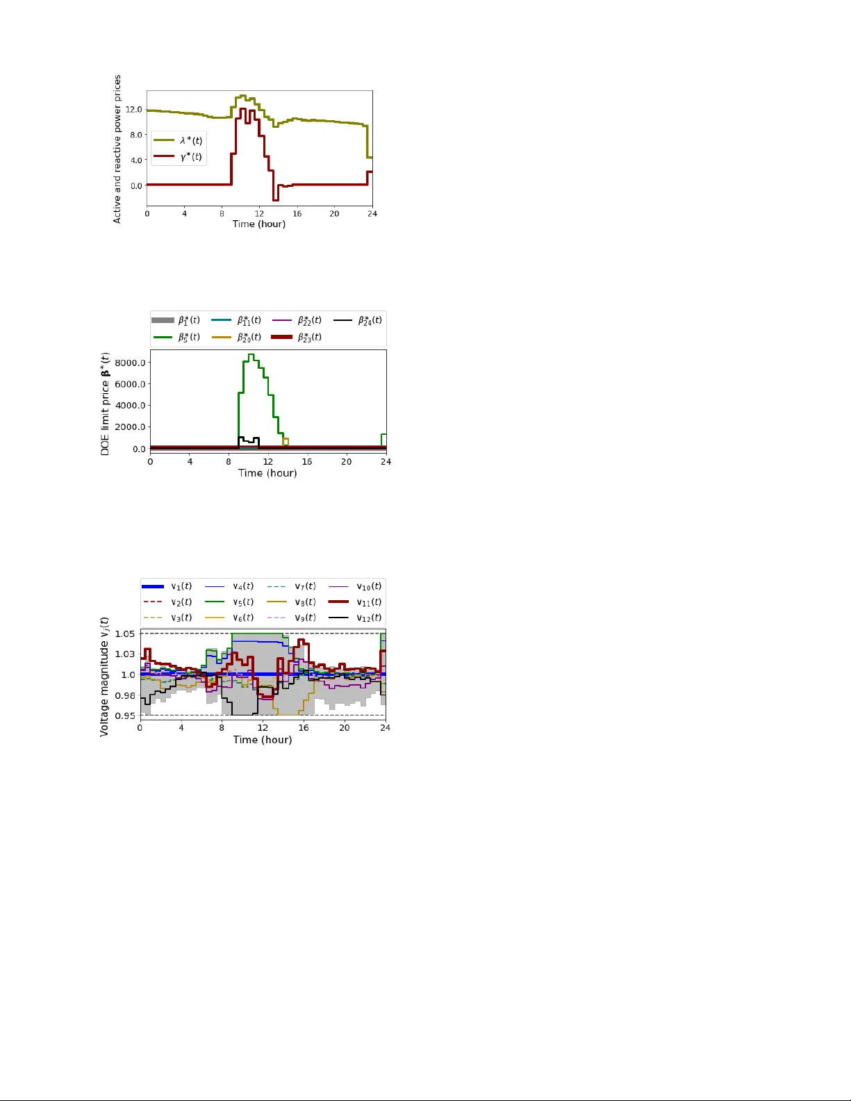
An Electricity Market with Reacti ve P o wer T rading: Incorporating Dynamic Operating En velopes Zeinab Salehi, Elizabeth L. Ratnam, Y ijun Chen, Ian R. Petersen, Guodong Shi, and Duncan S. Callaway Abstract — Electricity market design that accounts f or grid constraints such as voltage and thermal limits at the distrib u- tion level can increase opportunities for the grid integration of Distributed Ener gy Resources (DERs). In this paper , we consider rooftop solar backed by battery storage connected to a distribution grid. W e design an electricity market to support customers sharing rooftop generation in excess of their energy demand, wher e customers earn a pr ofit through peer -to-peer (P2P) energy trading. Our proposed electricity market also incorporates P2P reactiv e power trading to impro ve the voltage profile across a distribution feeder . W e formulate the electricity market as an optimization-based problem, where voltage and thermal limits across a feeder are managed through the assignment of customer-specific dynamic operating en velopes (DOEs). The electricity market equilibrium is referr ed to as a competitive equilibrium, which is equiv alent to a Nash equilibrium in a standard game. Our proposed market design is benchmarked using the IEEE 13-node test feeder . I . I N T RO D U C T I O N Power systems are transitioning from centralized fossil fuel-based generation to renew able-based operations — with a more geographically distributed energy mix. An element of the energy transition is the recent rapid uptake of distributed energy resources (DERs), including rooftop solar back ed by battery storage systems, and electric vehicles (EVs). As electricity end-users become equipped with DERs, providing the means to both consume and generate electricity (i.e., an energy prosumer), new opportunities arise to participate in electricity markets [1]. T o ef ficiently operate distrib ution net- works with gro wing populations of prosumers, new market mechanisms that support both energy trading and voltage regulation at the distribution-lev el are required [2]. An energy trading market operator in a competitiv e market determines the price for electricity , and sets the price accord- ing to the law of supply and demand [3], [4]. In a competiti ve energy market, prosumers are considered small relati ve to the market size, and accordingly , indi vidual decisions of This work w as supported by the Australian Research Council under grants DP190102158, DP190103615, LP210200473, and DP230101014. Zeinab Salehi and Ian R. Petersen are with the School of Engineering, Australian National University , Canberra, ACT 2601, Australia (e-mail: zeinab .salehi@anu.edu.au; ian.petersen@anu.edu.au). Elizabeth L. Ratnam is with the Department of Electrical and Computer Systems Engineering, Monash Uni versity , Melbourne, VIC 3168, Australia (e-mail: liz.ratnam@monash.edu). Y ijun Chen is with the Department of Electrical and Electronic En- gineering, University of Melbourne, VIC 3052, Australia (e-mail: yi- jun.chen.1@unimelb .edu.au). Guodong Shi is with the Australian Centre for Robotics, School of Aerospace, Mechanical and Mechatronic Engineering, The Univ ersity of Sydney , NSW 2050, Australia (e-mail: guodong.shi@sydney .edu.au). Duncan S. Callaway is with the Energy and Resources Group, Univ ersity of California, Berkeley , CA 94720 USA (e-mail: dcal@berkeley .edu). prosumers do not influence the price [3]. Once the market operator sets the electricity price, each prosumer seeks to maximize their payof f [5], a combination of the cost of electricity consumption and income from electricity trading. The market reaches a competitive equilibrium when no participant has an incentive to change their decision, and total supply matches total demand [6]–[8]. T o efficiently operate an electric grid, physics-based con- straints, including v oltage and thermal limits, must also be considered in the design of a new market mechanism. Distribution Network Service Providers (DNSPs) typically impose static limits on customer imports and exports to ensure feeder-le vel voltage and thermal limits remain within permissible operating env elopes. Howe ver , static import and export limits are conserv ativ e, as they do not reflect time- varying grid conditions [9]. Accordingly , DNSPs are in- creasingly adopting flexible grid connection agreements with prosumers, supporting operations with Dynamic Operating En velopes (DOEs) [10]. Specifically , a DOE is computed by a DNSP and is communicated to a prosumer — providing a range of permissible activ e and reactive po wer injections (or demand) at a given time [11]. Ancillary services are another element of an electric- ity market, impro ving the reliability and security of the electricity supply . Ancillary services have typically been provided by large, centralized generators. As we transition to renewable-based grid operations, ancillary services are increasingly being deli vered by a wider range of partici- pants, including prosumers with DERs [12]. Key ancillary services include frequency regulation [13], voltage support [2], and black-start capability [14]. That is, within DOE limits, prosumers can contribute to both energy trading and ancillary services. Ho wev er , limited DOE implementation and insufficient incenti ves for prosumer-based reacti ve power regulation potentially reduce the ef ficiency of existing mark et operations [15], [16]. In this paper , we consider a radial distribution grid that connects customers with DERs, including rooftop solar , battery storage, and EVs. W e assume prosumers regulate both real and reactiv e po wer via inv erters to support energy trading and grid constraints such as voltage and thermal limits. W e design a P2P ener gy market that enables both activ e power and reactive power trading between prosumers, achieving a balance in electricity supply and demand. Build- ing on our prior work in [17], we ensure grid constraints are satisfied by localizing feeder-le vel grid constraints into prosumer lev el DOE constraints. T o improv e the o verall utilization of the feeder , we design a market-mechanism whereby prosumers trade any excess DOE capacity , which would otherwise remain unused. The main contributions of the paper are summarized in the following. • W e design an energy market with activ e and reactiv e power trading and DOE limit trading. • W e show that the market equilibrium is a competitiv e equilibrium and maximizes social welfare, defined as the sum of the utilities of all customers. • W e show that the proposed markets can be represented as a standard game, where prosumers are the players and a fictitious price-setting player determines the price, with the solution concept being a Nash equilibrium. The rest of the paper is organized as follows. Section II introduces the prosumer dynamics and DOE constraints. Sec- tion III formulates the electricity market with reactiv e power trading to operate within feeder-le vel constraints. Section IV in vestigates the relation of the proposed market with the Nash equilibrium of a standard game. Section V presents numerical simulation results and Section VI concludes the paper . I I . P R E L I M I NA R I E S W e consider an electrical distribution feeder with a ra- dial topology connecting N prosumers, each equipped with rooftop solar backed by battery storage. W e consider the case where the electrical feeder operates in an island mode to support the blackstart capability of the bulk grid, i.e., all demand is met through local generation and P2P trading. W e assume each prosumer has a home ener gy management system (EMS) that manages the rate of electricity consump- tion and energy trading according to the preferences of the prosumer . W ithin the EMS, the prosumer preferences are formulated into mathematical expressions termed the payoff, which is defined as the sum of the consumption utility (satisfaction le vel) and the income or expenditure from energy trading. Each prosumer i , indexed in the set N = { 1 , . . . , N } , has uncontrollable loads such as lighting, and controllable loads such as EVs and home battery storage systems. The net supply of each prosumer i is defined as the dif ference between the rooftop solar generation and uncontrollable load and is denoted by a i ( t ) ∈ R (kW). Controllable loads are modeled by linear difference equations x i ( t + 1) = A i x i ( t ) + B i u i ( t ) , t ∈ T , (1) where x i ( t ) ∈ R n is the dynamical state (e.g., the state of charge (SoC) of a battery), x i (0) ∈ R n is the initial state (e.g., the initial SoC of a battery), and u i ( t ) ∈ R m is the control input (e.g., the charge/discharge rate of a battery). Also, A i ∈ R n × n and B i ∈ R n × m are fixed matrices. States and control inputs are constrained by x i ≤ x i ( t ) ≤ x i and u i ≤ u i ( t ) ≤ u i , where x i ∈ R n and u i ∈ R m denote lower bounds, and x i ∈ R n and u i ∈ R m denote upper bounds. Prosumer preferences for managing controllable loads are expressed by utility functions f i ( x i ( t ) , u i ( t )) : R n × R m 7→ R that represent their satisfaction as a result of taking the control action u i ( t ) and reaching the state x i ( t ) . F or example, if the SoC of the battery is close to 80% and the number of char ge/discharge cycles are relati vely lo w , then the prosumer potentailly achiev es a high level of satisfaction and a high f i ( · ) . Similarly , the terminal utility of a prosumer at the terminal time step T is denoted by ϕ i ( x i ( T )) : R n 7→ R , which depends on their satisfaction as a result of reaching the terminal state x i ( T ) . The av erage active power consumed or withdrawn as a result of the control action u i ( t ) is denoted by h i ( u i ( t )) : R m 7→ R (kW). At each time step t , if an agent i has a supply shortage, i.e., a i ( t ) − h i ( u i ( t )) < 0 , it can purchase the deficit from others; con versely , if it has a surplus, it can sell it to others through a trading decision variable p i ( t ) ∈ R (kW) such that p i ( t ) ≤ a i ( t ) − h i ( u i ( t )) 1 . Activ e power injection is also constrained by inv erter limits such that p i ≤ p i ( t ) ≤ p i , where p i and p i denote the lower and upper bound inv erter limits, respecti vely . Behind-the-meter inv erters with reacti ve power regulation capability can support voltage re gulation grid services. The injected or absorbed reactive po wer by prosumer i is denoted by q i ( t ) ∈ R (kV ar) such that q i ≤ q i ( t ) ≤ q i , where q i and q i represent the lower and upper bound in verter limits, respectiv ely . All inv erter-based voltage regulation across a distribution feeder must comply with physics-based grid limits. A. Electric Grid Constraints Denote p ( t ) = ( p 1 ( t ) , . . . , p N ( t )) ⊤ and q ( t ) = ( q 1 ( t ) , . . . , q N ( t )) ⊤ as the vectors of acti ve and reactiv e power injections of all prosumers at time step t ∈ T , respectiv ely . W e represent grid constraints in the separable form [11] F t ( p ( t ) , q ( t )) = N X i =1 g it ( p i ( t ) , q i ( t )) ≤ ν ( t ) , t ∈ T , (2) where F t : R N × R N 7→ R M is an af fine vector function, and M denotes the total number of grid constraints at time step t ∈ T . Each function g it : R × R 7→ R M is a local affine vector function associated with prosumer i capturing its contribution to the M global grid constraints at time step t ∈ T . These functions are determined by grid characteristics such as line impedances and topology . The vector ν ( t ) ∈ R M specifies the bounds on the grid constraints, deriv ed by the physical and operational limits of the netw ork. T w o examples of constraints expressed in the form of (2) include v oltage and thermal limits [11]. Details of voltage constraints are provided in [11], [17]. Enforcing the grid constraints in (2) requires assigning feasible operating limits to individual prosumers. Static export limits or fixed po wer factor settings are often too conservati ve, as they fail to reflect the time-varying network conditions. DOEs hav e emerged as a promising approach to address this challenge. Definition 1 (as in [11]): A DOE is a nonempty , closed, and con vex set Ω it ⊆ R 2 in the ( p i ( t ) , q i ( t )) space, that specifies an admissible region of active and reactiv e 1 This inequality applies to both surplus and deficit cases. power injections for prosumer i at time t , that the grid can accommodate without violating operational and physical constraints. Using the right-hand side decomposition (RHSD) method [18], the right-hand side of (2) can be expressed as ν ( t ) = P N i =1 w i ( t ) , where w i ( t ) ∈ R M represents the share of the M grid constraints assigned to prosumer i at time step t . Consequently , the grid constraints in (2) can be written as P N i =1 g it ( p i ( t ) , q i ( t )) ≤ P N i =1 w i ( t ) , which, when de- composed, yields the DOEs Ω it =  ( p i ( t ) , q i ( t )) ∈ R 2 : g it ( p i ( t ) , q i ( t )) ≤ w i ( t )  for each prosumer i ∈ N at time step t ∈ T [11]. There are infinitely many possible choices for the RHSD and DOEs. In this paper, we focus on an allocation that maximizes the potential activ e power injection to the grid, by solving max w ( t ) , p ( t ) , q ( t ) N X i =1 max { 0 , p i ( t ) } − ϵO ( w ( t )) s . t . g it ( p i ( t ) , q i ( t )) ≤ w i ( t ) N X i =1 w i ( t ) = ν ( t ) , i ∈ N , (3) where w ( t ) = ( w ⊤ 1 ( t ) , . . . , w ⊤ N ( t )) ⊤ , and ϵO ( w ( t )) is a regularization term with ϵ being a small positi ve num- ber . The function O ( w ( t )) : R N M 7→ R captures the preferences of the network service provider in allocat- ing DOE shares among prosumers. T o promote f airness, we consider O ( w ( t )) = ∥ w ( t ) − E ∥ , where E ∈ R N M , E = ( ν ⊤ ( t ) / N , . . . , ν ⊤ ( t ) / N ) ⊤ is the equality inde x. This choice of O ( w ( t )) reflects that the network service provider tends to allocate close to equal DOEs to all prosumers [11]. Solving (3), the network service provider determines the optimal DOEs and communicates them to each prosumer i in the form of g it ( p i ( t ) , q i ( t )) ≤ w ∗ i ( t ) . I I I . M A R K E T W I T H R E A C T I V E P OW E R C O M P E N S A T I O N Prosumers connected to the islanded feeder need to share their resources to meet their d e mand. In this section, we formulate a P2P ener gy market with reacti ve po wer trading that f acilitates this interaction. Let λ ( t ) ∈ R denote the price for activ e power trading and γ ( t ) ∈ R the price for reactiv e power trading at time step t . In our prior work [17], we showed that prosumers can also trade their excess DOE limits, i.e., w ∗ i ( t ) − g it ( p i ( t ) , q i ( t )) , through a decision variable l i ( t ) ∈ R M at a price β ( t ) ∈ R M , subject to l i ( t ) ≤ w ∗ i ( t ) − g it ( p i ( t ) , q i ( t )) , which mitigates the conserv atism introduced by decomposing global grid constraints into local DOEs. In the follo wing, we design a market that allows real and reactiv e power trading as well as DOE limit trading. Obtaining DOE limits w ∗ i ( t ) from (3), the coordinator determines equilibrium prices for acti ve power trading λ ∗ ( t ) , reactiv e po wer trading γ ∗ ( t ) , and DOE limit trading β ∗ ( t ) that clear the market for t ∈ T , and broadcasts them to par - ticipants. Upon receiving the equilibrium prices, prosumers engage in a P2P competiti ve mark et to maximize their payof f, defined as the sum of their utility f i ( x i ( t ) , u i ( t )) , terminal Fig. 1: Modified IEEE 13-node test feeder . Left: A prosumer i is zoomed in. utility ϕ i ( x i ( T )) , and the income λ ( t ) p i ( t ) + γ ( t ) q i ( t ) + β ( t ) · l i ( t ) from transactions. The mark et reaches an equilibrium when no participant has an incentive to change their decision and total supply equals total demand, i.e., the market clears. This equilibrium is called a competitive equilibrium , defined as follo ws. Let p i = ( p i (0) , . . . , p i ( T − 1)) ⊤ , q i = ( q i (0) , . . . , q i ( T − 1)) ⊤ , L i = ( l ⊤ i (0) , . . . , l ⊤ i ( T − 1)) ⊤ , and U i = ( u ⊤ i (0) , . . . , u ⊤ i ( T − 1)) ⊤ denote, respecti vely , the vectors of active power in- jections, reacti ve power injections, traded DOE limits, and control inputs of prosumer i o ver the entire time horizon. Definition 2: Optimal decisions ( u ∗ 1 ( t ) , p ∗ 1 ( t ) , q ∗ 1 ( t ) , l ∗ 1 ( t ) , . . . , u ∗ N ( t ) , p ∗ N ( t ) , q ∗ N ( t ) , l ∗ N ( t )) , along with optimal prices λ ∗ ( t ) , γ ∗ ( t ) , and β ∗ ( t ) for all t ∈ T , form a competitive equilibrium if the following statements hold. (i) Giv en λ ∗ ( t ) , γ ∗ ( t ) , β ∗ ( t ) , and w ∗ i ( t ) , each prosumer i ∈ N maximizes their payoff at ( u ∗ i ( t ) , p ∗ i ( t ) , q ∗ i ( t ) , l ∗ i ( t )) for t ∈ T as a solution to max U i , p i , q i , L i T − 1 X t =0  f i ( x i ( t ) , u i ( t )) + λ ∗ ( t ) p i ( t ) + γ ∗ ( t ) q i ( t ) + β ∗ ( t ) · l i ( t )  + ϕ i ( x i ( T )) s . t . x i ( t + 1) = A i x i ( t ) + B i u i ( t ) , p i ( t ) ≤ a i ( t ) − h i ( u i ( t )) , l i ( t ) ≤ w ∗ i ( t ) − g it ( p i ( t ) , q i ( t )) , x i ≤ x i ( t ) ≤ x i , u i ≤ u i ( t ) ≤ u i , p i ≤ p i ( t ) ≤ p i , q i ≤ q i ( t ) ≤ q i , t ∈ T . (4) (ii) All traded power and all traded DOE limits are balanced at each time step; that is, N X i =1 p ∗ i ( t ) = 0 , N X i =1 q ∗ i ( t ) = 0 , N X i =1 l ∗ i ( t ) = 0 , t ∈ T . (5) From microeconomics theory , a market outcome is Pareto efficient if there is no waste in the allocation of resources. Mathematically , a market outcome ( u ⋆ 1 ( t ) , p ⋆ 1 ( t ) , q ⋆ 1 ( t ) , l ⋆ 1 , . . . , u ⋆ N ( t ) , p ⋆ N ( t ) , q ⋆ N ( t ) , l ⋆ N ) for all t ∈ T is ef ficient if it maximizes the social welfare of the society , defined as the sum of all participant utilities f i ( · ) and ϕ i ( · ) , subject to local and global constraints. Such an operating point ( u ⋆ 1 ( t ) , p ⋆ 1 ( t ) , q ⋆ 1 ( t ) , l ⋆ 1 , . . . , u ⋆ N ( t ) , p ⋆ N ( t ) , q ⋆ N ( t ) , l ⋆ N ) for all t ∈ T is referred to as a social welfar e maximization solution and solves max U , P , Q , L N X i =1  T − 1 X t =0 f i ( x i ( t ) , u i ( t )) + ϕ i ( x i ( T ))  s . t . x i ( t + 1) = A i x i ( t ) + B i u i ( t ) , p i ( t ) ≤ a i ( t ) − h i ( u i ( t )) , l i ( t ) ≤ w ∗ i ( t ) − g it ( p i ( t ) , q i ( t )) , N X i =1 p i ( t ) = 0 , N X i =1 q i ( t ) = 0 , N X i =1 l i ( t ) = 0 , x i ≤ x i ( t ) ≤ x i , u i ≤ u i ( t ) ≤ u i , p i ≤ p i ( t ) ≤ p i , q i ≤ q i ( t ) ≤ q i , i ∈ N , t ∈ T , (6) where P = ( p ⊤ 1 , . . . , p ⊤ N ) ⊤ , Q = ( q ⊤ 1 , . . . , q ⊤ N ) ⊤ , L = ( L ⊤ 1 , . . . , L ⊤ N ) ⊤ , and U = ( U ⊤ 1 , . . . , U ⊤ N ) ⊤ denote, respec- tiv ely , the vectors of all acti ve power injection, reacti ve power injection, traded DOE limits, and control inputs of all prosumers over the entire time horizon. In the follo wing theorem, we show that the market out- come in Definition 2 is P areto efficient, maximizing (6). Theor em 1: Suppose f i ( · ) , ϕ i ( · ) , and − h i ( · ) are concav e functions for i ∈ N , and Slater’ s condition holds for (4) and (6). Given feasible initial conditions x i (0) for i ∈ N , the following statements hold. • A competitive equilibrium in Definition 2 is equiv alent to a social welfare maximization solution to (6). • Let − α ∗ ( t ) , − ϑ ∗ ( t ) , and − δ ∗ ( t ) be optimal dual variables corresponding to the balancing equality con- straints P N i =1 p i ( t ) = 0 , P N i =1 q i ( t ) = 0 , and P N i =1 l i ( t ) = 0 in (6), respectively , for t ∈ T . Then, equilibrium prices can be obtained as λ ∗ ( t ) = α ∗ ( t ) , γ ∗ ( t ) = ϑ ∗ ( t ) , and β ∗ ( t ) = δ ∗ ( t ) for t ∈ T . Pr oof: See Appendix I. A procedure for implementing the proposed P2P market in Definition 2 is described in Algorithm 1. Algorithm 1 Implementation of the P2P Market 1: DNSP determines DOEs by solving (3) and sends w ∗ i ( t ) to each prosumer i . 2: DNSP computes market prices λ ∗ ( t ) , γ ∗ ( t ) , and β ∗ ( t ) as the optimal dual variables corresponding to the balancing constraints in (6), and broadcasts them to prosumers. 3: Prosumers form a P2P market and trade resources to maximize their payoff in (4). Remark 1: Although Algorithm 1 employs a centralized approach in Step 2 to determine market prices, decentralized alternativ es such as the Alternating Direction Method of Multipliers (ADMM) or dual decomposition can also be applied, as in [19], [20]. In these methods, prosumers obtain resource prices in a decentralized manner , either with or without the supervision of a central coordinator . Following a procedure similar to [20], a fully decentralized and iterati ve scheme based on the dual decomposition method can be established for the P2P market proposed in Definition 2. In a fully decentralized P2P frame work, prosumers independently determine resource prices, and all information exchange occurs among neighboring participants without central co- ordination. Such approaches preserve participant priv acy . I V . N A S H E Q U I L I B R I U M In this section, we examine the connection between the proposed mark et and a standard game. W e show that the market outcome in Definition 2 can be implemented as a Nash equilibrium of a standard game with N + 1 players. • The first player is an aggregator who takes the role of a price player and regulates the price such that the market clears. Gi ven p i ( t ) , q i ( t ) , and l i ( t ) for i ∈ N and t ∈ T , the price player obtains uniform prices λ ( t ) , γ ( t ) , and β ( t ) as a solution to max λ , γ , β N X i =1 T − 1 X t =0  − λ ( t ) p i ( t ) − γ ( t ) q i ( t ) − β ( t ) · l i ( t )  , (7) where λ = ( λ (0) , . . . , λ ( T − 1)) ⊤ , γ = ( γ (0) , . . . , γ ( T − 1)) ⊤ , and β = ( β ⊤ (0) , . . . , β ⊤ ( T − 1)) ⊤ are the vectors of all activ e power , reactiv e power , and DOE limit prices o ver the entire time horizon, respectiv ely . • The last N players are prosumers who maximize their payoff subject to the local constraints. Gi ven prices λ ( t ) , γ ( t ) , and β ( t ) for t ∈ T , each prosumer i ∈ N obtains ( U i , p i , q i , L i ) as a solution to max U i , p i , q i , L i T − 1 X t =0 f i ( x i ( t ) , u i ( t )) + ϕ i ( x i ( T )) + T − 1 X t =0  λ ( t ) p i ( t ) + γ ( t ) q i ( t ) + β ( t ) · l i ( t )  s . t . x i ( t + 1) = A i x i ( t ) + B i u i ( t ) , p i ( t ) ≤ a i ( t ) − h i ( u i ( t )) , l i ( t ) ≤ w ∗ i ( t ) − g it ( p i ( t ) , q i ( t )) , x i ≤ x i ( t ) ≤ x i , u i ≤ u i ( t ) ≤ u i , p i ≤ p i ( t ) ≤ p i , q i ≤ q i ( t ) ≤ q i , t ∈ T . (8) The standard game in (7)–(8) stems from the generalized game introduced in [4], where the objective function of the price player indicates the “law of supply and demand”. Theor em 2: Let ( U ∗ , P ∗ , Q ∗ , L ∗ ) , along with λ ∗ ( t ) , γ ∗ ( t ) , β ∗ ( t ) for t ∈ T , be a Nash equilibrium for the standard game in (7)–(8). Then ( U ∗ , P ∗ , Q ∗ , L ∗ ) , along with λ ∗ ( t ) , γ ∗ ( t ) , β ∗ ( t ) for t ∈ T , is equiv alent to a competiti ve equilibrium as defined in Definition 2. Pr oof: A Nash equilibrium is obtained when P N i =1 p ∗ i ( t ) = 0 , P N i =1 q ∗ i ( t ) = 0 , and P N i =1 l ∗ i ( t ) = 0 for t ∈ T , and therefore, the objecti ve of the first player in (7) has a finite solution. This is equiv alent to the second condition in Definition 2. Additionally , a Nash equilibrium is obtained when the objectiv e of the last N players in (8) is maximized, which corresponds to the first condition in Definition 2. Consequently , it is straightforward to show that ( U ∗ , P ∗ , Q ∗ , L ∗ ) , along with λ ∗ ( t ) , γ ∗ ( t ) , β ∗ ( t ) for t ∈ T , satisfies all the conditions in Definition 2. Furthermore, all competitive equilibria in Definition 2 serve as a Nash equilibrium for the game defined by (7)–(8). V . N U M E R I C A L S I M U L A T I O N S In this section, we benchmark the proposed market with reactiv e po wer trading against one without reacti ve power participation. For simplicity , we consider voltage constraints in the electric grid; extensions to include thermal constraints are straightforw ard. W e use a modified single-phase rep- resentation of the IEEE 13-node test feeder, as shown in Fig. 1, where the transformer between nodes 2 and 3, the switch between nodes 6 and 7, and all capacitor banks are omitted [21]. All simulations are conducted in Python 3.8 using CVXPY on a MacBook Pro with an Apple M1 chip and 16 GB of memory . A. Simulation Setup Apart from the feeder node, node 1, and node 6, each node is connected to 30 distribution aggregators. Each aggregator manages 11 residential prosumers, each equipped with a grid-connected EV and a home battery storage system. The net po wer supply of each prosumer —defined as rooftop solar generation minus uncontrollable demand—is deri ved from metering data provided by Ausgrid [22], an Australian electricity distribution network provider . This dataset, orig- inally collected in 2012, is scaled by a factor of 2 to reflect increased solar generation and electrification lev els. EV models are from a di verse set documented in [23], with battery capacities ranging from 0 to 75 (kWh). The corresponding home battery storage systems are assumed to hav e similar capacity characteristics. The char ge/discharge efficiencies of EVs and home battery storage systems are assumed to be η = 0 . 9 . The system is simulated over a 24 - hour (h) time horizon starting at midnight, with a sampling time of ∆ = 0 . 5 (h). The aggregated behavior of each aggregator i , incor - porating both EVs and home battery storage systems of the associated 11 prosumers, is modeled using the linear difference equation x i ( t + 1) = x i ( t ) + η u i ( t )∆ , where x i ( t ) ∈ R 2 denotes the SoC vector (kWh) of the aggregated EVs and residential battery storage systems, and u i ( t ) ∈ R 2 represents the corresponding charge/discharge rate vector (kW) at each time step t . In both vectors, the first element corresponds to the aggregated EVs, and the second to the aggregated home battery storage systems. The initial SoC of each battery is assumed to follow a uniform distribution over the interv al [0 . 2 , 0 . 5] of its respecti ve capacity . Home battery storage systems remain grid-connected at all times, whereas EV arri val and departure times are drawn from surve y data collected by the V ictorian Department of T ransport in Australia [24]. Prosumers are assumed to use le vel- 2 chargers with a maximum charge rate of 6 . 6 (kW) [21], and a corresponding maximum discharge rate of − 6 . 6 (kW). T o preserve battery health, the SoC of both EVs and home battery storage systems is constrained to remain between 20% and 85% of their respective capacities. Accordingly , the aggregated SoC and charging/dischar ging rates for each aggregator i are bounded by 0 . 2 C i ≤ x i ( t ) ≤ 0 . 85 C i and − 6 . 6 1 ≤ u i ( t ) ≤ 6 . 6 1 , respectiv ely , where C i ∈ R 2 denotes the v ector of aggre gated battery capacities (kWh) and 1 ∈ R 2 is a vector of ones. The first and second elements of C i correspond to the aggregated EV and home battery capacities, respectiv ely , of the prosumers managed by aggregator i . Prosumers hav e in verters with reacti ve po wer import and export limits of 0 . 33 kV ar . In this framework, each of the N = 300 aggregators functions as a decision-maker , approximating the aggreg ate behavior of its associated prosumers. The utility function for aggregator i ∈ N is defined as a quadratic form 2 f i ( x i ( t ) , u i ( t )) = − ϑ 1 ∥ u i ( t ) ∥ 2 − ϑ 2 ,t ∥ ( x i ( t ) − 0 . 85 C i ) · (1 , 0) ⊤ ∥ 2 − ϑ 3 ,t ∥ ( x i ( t ) − 0 . 85 C i ) · (0 , 1) ⊤ ∥ 2 for t ∈ T = { 0 , . . . , 47 } , where ∥ · ∥ denotes the Euclidean norm. The terminal utility is gi ven by ϕ i ( x i ( T )) = − ϑ 4 ∥ x i ( T ) − 0 . 85 C i ∥ 2 , with T = 48 as the terminal time step. The coefficients ϑ 1 ( 10 − 8 ¢/(kW) 2 ), ϑ 2 ,t ( 10 − 8 ¢/(kWh) 2 ), ϑ 3 ,t ( 10 − 8 ¢/(kWh) 2 ), and ϑ 4 ( 10 − 8 ¢/(kWh) 2 ) serve as regular- ization weights. For each aggregator i , the power consumed or withdrawn by the aggregated controllable loads (EVs and home battery storage systems) is modeled as h i ( u i ( t )) = u i ( t ) · 1 . The feeder nominal v oltage is set to V 0 = 1 (p.u.). In compliance with the ANSI C84.1 standard, voltage magnitudes must remain within ± 5% of the nominal voltage. B. Numerical Simulations Considering voltage constraints, the DNSP obtains DOEs according to (3), and sends the obtained w ∗ i ( t ) to each aggregator i for i ∈ { 1 , . . . , 300 } . The DNSP sends the activ e and reacti ve po wer prices, λ ∗ ( t ) and γ ∗ ( t ) , and DOE limit prices β ∗ ( t ) , which could be obtained solving (6), to each aggregators. Each aggregator i then decides on its electricity consumption and trading to maximize its payoff according to (4). The active and reactive power prices are depicted in Fig. 2, and the DOE limit prices are shown in Fig. 3. Zero and neg ativ e reacti ve po wer prices in Fig. 2 cor- respond to cases where reactive po wer is in excess in the grid and must be absorbed by inv erters. Similarly , zero prices for different elements of DOE limit trading in Fig. 3 indicate that the associated v oltage constraints remain within their boundaries, whereas nonzero prices correspond to cases where the respectiv e voltages reach the boundary . The nodal voltages are sho wn in Fig. 4 and compared with the case without reactive po wer injection (gray area). As observed, reactiv e power trading functions as an ancillary service mar- ket that improves voltage regulation, with voltages reaching their boundaries less frequently . Moreover , we observed that 2 The utility function can take any form, the only requirement is that it is concav e. Fig. 2: Acti ve po wer prices λ ∗ ( t ) (¢/kWh) and reacti ve po wer prices γ ∗ ( t ) (¢/kV arh), ov er a 24-hour period (48 time steps of length 0 . 5 hour). Fig. 3: Some elements of the DOE limit price vector β ∗ ( t ) (in ¢/(kV) 2 ) over a 24-hour period (48 time steps of length 0 . 5 hour). The k -th element of β ∗ ( t ) is denoted by β ∗ k ( t ) . The other 17 elements are close to zero and not depicted. Fig. 4: Nodal voltages v j ( t ) (p.u.) for each of the 12 nodes, j ∈ { 1 , . . . , 12 } . The gray area indicates the voltage range without reactiv e power trading across the grid. reactiv e power trading increases community profit, as the social welfare of the system rises by 1 . 6% compared to the case without reactiv e power trading. V I . C O N C L U S I O N W e considered a radial distribution feeder operating in island mode to support the blackstart capability of the bulk grid. W e designed a peer-to-peer energy market to enable energy trading by prosumers with behind-the-meter rooftop solar backed by battery storage. Moreo ver , we design the market to incorporate v oltage regulation across the feeder by way of in verter-based resources regulating reactive power flows to and from prosumers. Specifically , we decomposed power flo w constraints across the feeder into localized customer-le vel limits, termed dynamic operating en velopes (DOEs). W e showed that our proposed market maximizes social welfare and is equi valent to a standard game. W e benchmarked our proposed market using the IEEE 13-node test feeder under binding voltage constraints. Our results demonstrate that reacti ve po wer trading functions as an ancil- lary service market, improving both the community’ s welfare and the ov erall voltage profile of the feeder compared to the case without reactiv e power trading. Future work to consider heterogeneous prosumer utility functions is possible. R E F E R E N C E S [1] M. I. Azim et al., “Dynamic operating en velope-enabled P2P trading to maximize financial returns of prosumers, ” IEEE T ransactions on Smart Grid , vol. 15, no. 2, pp. 1978–1990, March 2024. [2] Y . Meng, J. Qiu, C. Zhang, G. Lei, and J. Zhu, “ A Holistic P2P market for activ e and reactiv e energy trading in VPPs considering both financial benefits and network constraints, ” Applied Ener gy , vol. 356, p. 122396, 2024. [3] A. Mas-Colell, M. D. Whinston, and J. R. Green, Micr oeconomic Theory , vol. 1. New Y ork: Oxford Univ . Press, 1995. [4] K. J. Arro w and G. Debreu, “Existence of equilibrium for a compet- itiv e economy , ” Econometrica , vol. 22, no. 3, pp. 265–290, 1954. [5] F . Alfaverh, M. Denai, and Y . Sun, “ A dynamic peer-to-peer electricity market model for a community microgrid with price-based demand response, ” IEEE T ransactions on Smart Grid , vol. 14, no. 5, pp. 3976– 3991, Sept. 2023. [6] S. Li, J. Lian, A. J. Conejo, and W . Zhang, “T ransactiv e energy sys- tems: The market-based coordination of distributed energy resources, ” IEEE Contr ol Syst. Mag. , vol. 40, no. 4, pp. 26–52, Aug. 2020. [7] Z. Salehi, Y . Chen, E. L. Ratnam, I. R. Petersen, and G. Shi, “Com- petitiv e equilibrium for dynamic multiagent systems: Social shaping and price trajectories, ” IEEE T ransactions on Automatic Control , vol. 69, no. 8, pp. 5184–5199, Aug. 2024. [8] Z. Salehi, Y . Chen, E. L. Ratnam, I. R. Petersen, and G. Shi, “Competitiv e equilibriums of multi-agent systems over an infinite horizon, ” IF AC-P apersOnLine , vol. 56, pp. 37–42, 2023. [9] G. Lankeshwara, R. Sharma, R. Y an, T . K. Saha, and J. V . Milanovi ´ c, “T ime-varying operating regions of end-users and feeders in low- voltage distribution networks, ” IEEE T ransactions on P ower Systems , vol. 39, no. 2, pp. 4600–4611, March 2024. [10] CutlerMerz. Re view of dynamic operating en velopes adoption by DNSPs. Accessed: 2026. [Online]. A v ailable: https://arena.gov .au/assets/2022/07/revie w-of-dynamic-operating- en velopes-from-dnsps.pdf [11] M. Mahmoodi, L. Blackhall, S. M. Noori R. A., A. Attarha, B. W eise, and A. Bhardwaj, “DER capacity assessment of active distrib ution systems using dynamic operating env elopes, ” IEEE T ransactions on Smart Grid , vol. 15, no. 2, pp. 1778–1791, 2024. [12] L. Li, S. Fan, J. Xiao, Y . Zhang, R. Huang, and G. He, “Energy management strategy for community prosumers aggregated VPP par- ticipation in the ancillary services market based on P2P trading, ” Applied Ener gy , v ol. 384, p. 125472, 2025. [13] K. Li, L. W ei, J. Fang, X. Ai, S. Cui, M. Zhu, and J. W en, “Incentive- compatible primary frequency response ancillary service mark et mech- anism for incorporating diverse frequency support resources, ” Energy , vol. 306, 2024. [14] D. Aguilar-Dominguez, J. Ejeh, S. F . Brown, and A. D. F . Dunbar, “Exploring the possibility to provide black start services by using vehicle-to-grid”, Energy Rep. , vol. 8, pp. 74–82, Nov . 2022. [15] Y . Zou and Y . Xu, “DER-inv erter based reactive power ancillary service for supporting peer-to-peer transactiv e energy trading in distri- bution networks, ” IEEE T ransactions on P ower Systems , vol. 40, no. 1, pp. 753–764, Jan. 2025. [16] Z. Jiang and Y . Guo, “Bargaining-based approach for dynamic operat- ing envelope allocation in distribution networks, ” IEEE Tr ansactions on Smart Grid , vol. 16, no. 5, pp. 3588–3600, 2025. [17] Z. Salehi, Y . Chen, I. R. Petersen, G. Shi, Duncan S. Callaway , and E. L. Ratnam, “Peer-to-peer energy markets with uniform pricing: A dynamic operating envelope approach, ” 2025, [18] I. V . Konnov , “Right-hand side decomposition for variational inequal- ities, ” J. Optim. Theory Appl. , vol. 160, no. 1, pp. 221–238, 2014. [19] D. H. Nguyen, “Optimal Solution Analysis and Decentralized Mecha- nisms for Peer-to-Peer Energy Markets, ” IEEE T ransactions on P ower Systems , vol. 36, no. 2, pp. 1470–1481, March 2021. vol. 154, p. 109428, December 2023. [20] A. Paudel, M. Khorasany , and H. B. Gooi, “Decentralized local energy trading in microgrids with voltage management, ” IEEE Tr ans. Ind. Informat. , vol. 17, no. 2, pp. 1111–1121, Feb. 2021. [21] N. I. Nimalsiri, E. L. Ratnam, C. P . Mediwaththe, D. B. Smith, and S. K. Halgamuge, “Coordinated charging and discharging control of electric vehicles to manage supply voltages in distribution networks: Assessing the customer benefit, ” Appl. Energy , vol. 291, Jun. 2021, Art. no. 116857. [22] Ausgrid. Solar home electricity data. Accessed: 2026. [Online]. A vailable: http://linked.data.gov .au/dataset/energy/42966a8f-bc3c- 4bde-91d6-91bc5826aa21 [23] Battery Univ ersity . Bu-1003: Electric vehicle (EV). Accessed: 2025. [Online]. A vailable: https://batteryuniversity .com/article/bu- 1003-electric-vehicle-e v#google vignette [24] Y . W u, S. M. Aziz, and M. H. Haque, “Datasets on probability distributions of arriv al and departure times of priv ately used electric vehicles, ” Data in Brief , vol. 57, p. 110917, 2024. Accessed: 2025. [Online]. A vailable: https://data.mendeley .com/datasets/gphwn7sy5n/1 A P P E N D I X I P RO O F O F T H E O R E M 1 Let ( U ∗ , P ∗ , Q ∗ , L ∗ ) , along with λ ∗ ( t ) , γ ∗ ( t ) , and β ∗ ( t ) for t ∈ T , be a competiti ve equilibrium. Merging optimiza- tion problems in (4) for i ∈ N implies that ( U ∗ , P ∗ , Q ∗ , L ∗ ) maximizes the social welfare in (6). The proof of the rev erse direction is based on strong duality , which follows from the satisfaction of Slater’ s condi- tion. Considering the difference equation (1), the state x i ( t ) ev olves according to a linear combination of the initial state x i (0) and the control input U i such that x i ( t ) = A t i x i (0) + P t − 1 j =0 A t − j − 1 i B i u i ( j ) for t ∈ { 1 , 2 , ..., T } , whose substitu- tion into f i ( · ) and ϕ i ( · ) results in f i ( x i ( t ) , u i ( t )) = ˜ f i,t ( U i ) and ϕ i ( x i ( T )) = ˜ ϕ i ( U i ) . The functions ˜ f i,t ( · ) and ˜ Φ i ( · ) are concav e as the composition of a conca ve function and an affine function. For i ∈ N , denote U i = { U i | u i ≤ u i ( t ) ≤ u i ; x i ≤ x i ( t ) ≤ x i ; p i ≤ p i ( t ) ≤ p i ; q i ≤ q i ( t ) ≤ q i , for t ∈ T } , which is a polyhedral set. For any ( U , P , Q , L ) such that U i ∈ U i , the Lagrangian function of (6) is defined as L ( U , P , Q , L , α , ϑ , δ , Ψ , Π ) = − N X i =1  T − 1 X t =0 ˜ f i,t ( U i ) + ˜ ϕ i ( U i )  + T − 1 X t =0 α ( t )  − N X i =1 p i ( t )  + T − 1 X t =0 ϑ ( t )  − N X i =1 q i ( t )  + T − 1 X t =0 δ ( t ) ·  − N X i =1 l i ( t )  + T − 1 X t =0 N X i =1 ψ i ( t )  p i ( t ) + h i ( u i ( t )) − a i ( t )  , + T − 1 X t =0 N X i =1 π i ( t ) ·  l i ( t ) + g i ( p i ( t )) − w ∗ i ( t )  , (9) where ψ i ( t ) ≥ 0 , π i ( t ) ≥ 0 , α = ( α (0) , . . . , α ( T − 1)) ⊤ , ϑ = ( ϑ (0) , . . . , ϑ ( T − 1)) ⊤ , δ = ( δ ⊤ (0) , . . . , δ ⊤ ( T − 1)) ⊤ , Ψ i = ( ψ i (0) , . . . , ψ i ( T − 1)) ⊤ , and Ψ = ( Ψ ⊤ 1 , . . . , Ψ ⊤ N ) ⊤ . W e define Π i and Π in a similar way . The Lagrangian (9) is separable such that L ( U , P , Q , L , α , ϑ , δ , Ψ , Π ) = N X i =1 L i ( U i , p i , q i , L i , α , ϑ , δ , Ψ i , Π i ) , (10) where L i ( U i , p i , q i , L i , α , ϑ , δ , Ψ i , Π i ) = − T − 1 X t =0  ˜ f i,t ( U i ) + α ( t ) p i ( t ) + ϑ ( t ) q i ( t ) + δ ( t ) · l i ( t )  − ˜ ϕ i ( U i ) + T − 1 X t =0 ψ i ( t )  p i ( t ) + h i ( u i ( t )) − a i ( t )  + T − 1 X t =0 π i ( t ) ·  l i ( t ) + g i ( p i ( t )) − w ∗ i ( t )  . Let ( U ⋆ , P ⋆ , Q ⋆ , L ⋆ ) be an optimal primal solution to (6), and ( − α ∗ , − ϑ ∗ , − δ ∗ , Ψ ∗ , Π ∗ ) be an optimal dual solution. Giv en that Slater’ s condition is satisfied, strong duality implies ( U ⋆ , P ⋆ , Q ⋆ , L ⋆ ) ∈ arg min U , P , Q , L L ( U , P , Q , L , α ∗ , ϑ ∗ , δ ∗ , Ψ ∗ , Π ∗ ) , (11) for U i ∈ U i . Considering (10) and (11), there holds ( U ⋆ i , p ⋆ i , q ⋆ i , L ⋆ i ) ∈ arg min U i , p i , q i , L i L i ( U i , p i , q i , L i , α ∗ , ϑ ∗ , δ ∗ , Ψ ∗ i , Π ∗ i ) , (12) for U i ∈ U i . In addition, strong duality implies ( α ∗ , ϑ ∗ , δ ∗ , Ψ ∗ , Π ∗ ) ∈ arg max α , ϑ , δ , Ψ , Π min U , P , Q , L L ( U , P , Q , L , α , ϑ , δ , Ψ , Π ) = arg max α , ϑ , δ , Ψ , Π min U , P , Q , L N X i =1 L i ( U i , p i , q i , L i , α , ϑ , δ , Ψ i , Π i ) , and, therefore, ( Ψ ∗ i , Π ∗ i ) ∈ arg max Ψ i , Π i min U i , p i , q i , L i L i ( U i , p i , q i , L i , α ∗ , ϑ ∗ , δ ∗ , Ψ i , Π i ) , where the primal and dual v ariables are in their respecti ve domains. Considering λ ∗ ( t ) = α ∗ ( t ) , γ ∗ ( t ) = ϑ ∗ ( t ) , and β ∗ ( t ) = δ ∗ ( t ) for t ∈ T , the function L i ( U i , p i , q i , L i , α ∗ , ϑ ∗ , δ ∗ , Ψ i , Π i ) is the Lagrangian of (4). Therefore, ( Ψ ∗ i , Π ∗ i ) is an op- timal dual solution of (4). Giv en that Slater’ s condition is satisfied, strong duality implies that according to (12), ( U ⋆ , P ⋆ , Q ⋆ , L ⋆ ) is an optimal primal solution of (4) which satisfies (5). Consequently , ( U ⋆ , P ⋆ , Q ⋆ , L ⋆ ) , along with λ ∗ ( t ) = α ∗ ( t ) , γ ∗ ( t ) = ϑ ∗ ( t ) , and β ∗ ( t ) = δ ∗ ( t ) for t ∈ T , forms a competitiv e equilibrium.