DM4CT: Benchmarking Diffusion Models for Computed Tomography Reconstruction

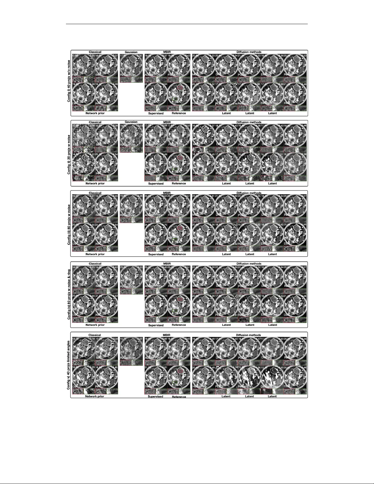
Published as a conference paper at ICLR 2026 D M 4 C T: B E N C H M A R K I N G D I FF U S I O N M O D E L S F O R C O M P U T E D T O M O G R A P H Y R E C O N S T R U C T I O N Jiayang Shi 1,2 , Dani ¨ el M. Pelt 1 , K. Joost Batenb urg 1 1 LIA CS, Leiden Uni versity 2 Centrum W iskunde en Informatica A B S T R AC T Diffusion models have recently emer ged as po werful priors for solving in v erse prob- lems. While c omputed tomography (CT) is theoretically a linear in v erse problem, it poses many practical challenges. These include correlated noise, artifact structures, reliance on system geometry , and misaligned v alue ranges, which make the direct application of dif fusion models more difﬁcult than in domains lik e natural image generation. T o systematically ev aluate how diffusion models perform in this context and compare them with established reconstruction methods, we introduce DM4CT , a compr ehensive benchmark for CT r econstruction . DM4CT includes datasets from both medical and industrial domains with sparse-vie w and noisy conﬁgurations. T o explore the challenges of deplo ying diffusion models in practice, we additionally acquire a high-resolution CT dataset at a high-energy synchrotron facility and ev aluate all methods under real experimental conditions. W e benchmark ten recent diffusion-based methods alongside se ven strong baselines, including model-based, unsupervised, and supervised approaches. Our analysis provides detailed insights into the behavior , strengths, and limitations of diffusion models for CT reconstruc- tion. The real-world dataset is publicly av ailable at zenodo.org/records/15420527, and the codebase is open-sourced at github .com/DM4CT/DM4CT. 1 I N T RO D U C T I O N Computed tomography (CT) is a typical example of an in verse problem, where the goal is to reconstruct an unknown object from indirect measurements (Sidky et al., 2020; Courdurier et al., 2008; Purisha et al., 2019). T echniques developed for CT reconstruction often extend to other in verse problems across v arious imaging applications (Clement et al., 2005; Mistretta et al., 2006; Dines & L ytle, 2005; Ladas & Dev aney, 1993). In many cases, the measurements are sparse or noisy , making the reconstruction problem ill-posed. This leads to ambiguity , as multiple solutions may ﬁt the measurements equally well. T o resolv e this, prior knowledge is typically incorporated. Approaches to utilize priors range from heuristic re gularizers, such as total v ariation (TV) (Sidky & Pan, 2008; Goris et al., 2012), to learned priors via supervised deep learning (Jin et al., 2017). Recently , dif fusion models have emerged as po werful generative models, achie ving remarkable success in text and image generation (W u et al., 2023c; Li et al., 2022; Nichol et al., 2021; Ho et al., 2022). Motiv ated by their expressi ve modeling capacity , many w orks have proposed to use dif fusion models as learned priors for in verse problems, sho wing promising results across a v ariety of domains (Chung et al., 2023; Song et al., 2024; Zirvi et al., 2025). Theoretically , CT reconstruction is a linear in verse problem and thus should beneﬁt from these advances. Howe ver , practical CT imaging introduces many additional challenges. Factors such as complex noise characteristics, nonlinear preprocessing steps like log transformation, and v arious artifacts result in real-world CT pipelines deviating substantially from the idealized linear model (Hendriksen et al., 2020). Therefore, a comprehensiv e and realistic benchmark is essential to rigorously e valuate dif fusion models for CT reconstruction and to compare them against other established CT reconstruction approaches. In this work, we introduce DM4CT , a benchmark designed to e valuate dif fusion-based methods for CT reconstruction. W e compare diffusion models with each other and against a range of strong, established baselines. As part of DM4CT , we also propose a uniﬁed taxonomy that or ganizes dif ferent dif fusion approaches based on their strategies for incorporating data consistenc y and prior kno wledge 1 Published as a conference paper at ICLR 2026 40 angles w/o noise 20 angles w mild noise 80 angles w more noise 80 angles w noise & ring artifacts 40 limited angles w/o noise Measurements … 10 representative di ﬀ usion methods + established methods Forward model … Output+evaluation Datasets noise & artifacts Medical CT : 2016 low dose grand challenge Industrial CT : LoDoInd Real-world dataset scanned at a synchrotron facility Conﬁgurations Qualitative metrics Quantitative metrics Visual comparison of reconstructions Image quality metrics Computation e ﬃ ciency metrics Real dataset sparse-view Reconstruction pipelines Noise Noise+ring (a) (b) (c) (d) Figure 1: Overvie w of the DM4CT benchmark. (a) The reconstruction pipeline, where representativ e dif fusion and baseline methods are applied to measured sinograms using the same forw ard model. (b) The datasets used in the benchmark, including two simulated CT datasets (medical and industrial) and one real-world dataset acquired at a synchrotron facility . (c) The ﬁve simulation conﬁgurations used to ev aluate robustness to limited vie ws, noise, and ring artifacts. T wo e xample FBP reconstructions under noise and ring artif act conditions are shown. (d) The ev aluation metrics, including both qualitativ e (visual) and quantitati ve (image quality and computational ef ﬁciency) criteria. (summarized in T able 1). The benchmark includes both medical and industrial CT datasets with controlled le vels of noise and artif acts for objecti ve, systematic comparison. In addition, we acquire a real-world dataset by scanning two rock samples at a synchrotron facility , allowing us to examine the limitations of deploying diffusion methods in practice under realistic conditions. An overvie w of our framew ork is illustrated in Figure 1. Our contributions: 1) W e present DM4CT , the ﬁrst systematic benchmark of diffusion models for CT reconstruction; 2) W e acquire and release a high-energy synchrotron CT dataset, offering a rare, well-suited resource for benchmarking under realistic conditions; 3) W e propose a uniﬁed taxonomy of dif fusion methods based on their strate gies for data consistency and prior knowledge (T able 1); 4) W e implement all benchmarked methods in the widely adopted dif fusers 1 framew ork and open-source the codebase; 5) W e perform extensi ve experiments pro viding practical insights into the strengths, limitations, and deployment challenges of dif fusion models in CT . W e emphasize that our goal is not to pr opose a new r econstruction algorithm, but to pr ovide the ﬁrst systematic benchmark for dif fusion models in CT . 2 P R E L I M I N A R I E S 2 . 1 C O M P U T E D T O M O G R A P H Y CT aims to recover an unkno wn object x ∈ R m from a set of projection measurements y ∈ R n . The measurement process can be mathematically modeled as a linear system y = Ax , (1) where A ∈ R n × m is the system matrix determined by the acquisition geometry . In practical settings, the measurements can be sparse (i.e., n < m ), leading to an underdetermined and ill-posed in verse problem. Furthermore, the measurements acquired during scanning are typically corrupted by noise. W e denote the actual observed measurements as e y ∈ R n . The discrepancy between the ideal and observed measurements describes the measurement noise ϵ = e y − y . The combination of sparsity and measurement noise poses signiﬁcant challenges for accurate image reconstruction in CT . T o address such challenges, prior knowledge is necessitated for the reconstruction. Classical methods often utilize heuristic priors such as T otal V ariation (TV) regularization (Sidk y & Pa n, 2008; Goris et al., 2012; Liu et al., 2013; Kazantsev et al., 2018), which assume image smoothness but lack 1 https://github.com/huggingface/diffusers 2 Published as a conference paper at ICLR 2026 domain-speciﬁc adaptability . Recent approaches lev erage data-driv en priors by training deep neural networks on paired sparse- and dense-view reconstruction images (Jin et al., 2017; Chen et al., 2017; Pelt et al., 2018; Zhang et al., 2021), capturing more expressiv e and task-speciﬁc features. Alternativ ely , implicit priors such as Deep Image Prior (DIP) (Ulyanov et al., 2018; Baguer et al., 2020; Barbano et al., 2022) and Implicit Neural Representations (INRs) (Sitzmann et al., 2020; Shen et al., 2022; W u et al., 2023b) regularize reconstruction through the neural network itself. 2 . 2 D I FF U S I O N M O D E L S W e brieﬂy revie w the two types of dif fusion models that are used as backbones in this work. Pixel Diffusion Models. W e consider Pixel-space Diffusion Probabilistic Models (DDPMs) (Ho et al., 2020; Nichol & Dhariwal, 2021) and view the forward diffusion and backward denoising processes as Stochastic Differential Equations (SDEs) (Song et al., 2020). In the forward process, Gaussian noise is gradually added to data x 0 ∼ p data such that, at a sufﬁciently lar ge time T , the perturbed variable x T approximates a Gaussian distribution x T ∼ N (0 , I ) . This process can be described by the V ariance-Preserving Stochastic Differential Equation (VP-SDE) (Song et al., 2020): d x = − β t 2 x + p β t d w , (2) where the β t is a time-dependent noise schedule, and d w denotes the standard Wiener process. The backward denoising process attempts to recov er samples from the original data distrib ution by gradually removing noise. This can be described by the corresponding re verse SDE (Anderson, 1982) d x = [ − β t 2 x − β t ∇ x t log p ( x t )] dt + p β t d ¯ w , (3) where d ¯ w is the rev erse-time W iener process, and ∇ x t log p ( x t ) is the score function of the interme- diate noisy distribution (Song & Ermon, 2019; 2020). A neural network is trained to approximate this score function, enabling sample generation by solving the rev erse SDE. Latent Diffusion Models. W e also consider Latent Diffusion Models (LDMs) (Rombach et al., 2022), which perform the forward dif fusion and rev erse denoising processes in a lower -dimensional latent space instead of the pixel space. The original data x is ﬁrst mapped to a latent representation via an encoder E , resulting in z = E ( x ) . The forward SDE is then applied in the latent space d z = − β t 2 z + √ β t d w . After the rev erse denoising process in the latent domain, a decoder D maps the denoised latent back to the data space. In our benchmark, we use a V ector Quantized V ariational Autoencoder (VQ-V AE) (V an Den Oord et al., 2017) as the encoder–decoder pair ( E , D ) following (Rombach et al., 2022; Rout et al., 2023; Song et al., 2024). 3 D M 4 C T T o apply diffusion models to in verse problems such as CT reconstruction, it is necessary to incorporate the measurement y into the re verse denoising process. From a Bayesian perspecti ve, the posterior distribution o ver the unkno wn image giv en the measurements is expressed as p ( x | y ) ∝ p ( x ) p ( y | x ) . This motiv ates a modiﬁcation of the reverse-time SDE (Equation 3) to a conditional re verse SDE: d x =  − β t 2 x − β t ( ∇ x t log p ( x t ) + ∇ x t log p ( y | x t ))  dt + p β t d ¯ w , (4) where ∇ x t log p ( x t ) is the score function approximated by the trained diffusion model, and ∇ x t log p ( y | x t ) introduces a measurement-informed correction. Howe ver , this measurement term is generally intractable, since y typically depends on the clean image x 0 rather than the noised version x t . A common strategy is to approximate the conditional term using the clean image estimate ˆ x 0 ( x t ) , ∇ x t log p ( y | x t ) ≈ ∇ x t log p ( y | ˆ x 0 ( x t )) . (5) There are two widely used estimators for ˆ x 0 ( x t ) , both deri ved from the dif fusion process. The ﬁrst is based on the DDPM formulation (Ho et al., 2020), ˆ x 0 = 1 √ ¯ α ( t ) ( x t − p 1 − ¯ α ( t ) ∇ x t log p ( x t )) . The second uses T weedie’ s formula (Song et al., 2020; Kim & Y e, 2021), which directly relates 3 Published as a conference paper at ICLR 2026 T able 1: Diffusion-based methods ev aluated in DM4CT . Columns under T echnique refer to implemen- tation choices (e.g., latent-space dif fusion or DDIM-based sampling). Columns under Reconstruction Strategy denote how measurement conditioning is incorporated, including data consistency gradient steering (DC-grad), separate optimization steps (DC-step), plug-and-play priors, and use of approxi- mate pseudoin verse solutions. A ✓ ∗ indicates only a single-step update tow ard the pseudoin verse. A ✓ ‡ indicates methods that incorporate data ﬁdelity via a conjugate-gradient solve rather than a direct pixel-space optimization step. Method Y ear T echnique Reconstruction Strategy Latent DDIM DC-grad DC-step Plug-and-Play Pseudo In v V ariational Bayes MCG (Chung et al., 2022) 2022 ✓ ∗ DPS (Chung et al., 2023) 2023 ✓ PSLD (Rout et al., 2023) 2023 ✓ ✓ PGDM (Song et al., 2023a) 2023 ✓ DDS (Chung et al., 2024) 2024 ✓ ✓ ‡ Resample (Song et al., 2024) 2024 ✓ ✓ ✓ ✓ DMPlug (W ang et al., 2024) 2024 ✓ ✓ ✓ Reddiff (Mardani et al., 2024) 2024 ✓ ✓ ✓ ✓ HybridReg (Dou et al., 2025) 2025 ✓ ✓ ✓ ✓ DiffStateGrad (Zirvi et al., 2025) 2025 ✓ ✓ ✓ ✓ the posterior mean to the score function: ˆ x 0 = 1 √ ¯ α ( t ) ( x t − (1 − ¯ α ( t )) ∇ x t log p ( x t )) , where ¯ α ( t ) = Q t j =1 (1 − β j ) is the cumulati ve noise schedule. These approximations enable conditioning on the measurement y during the re verse denoising process in a tractable way , forming the basis for a variety of measurement-a ware dif fusion reconstruction methods. 3 . 1 D I FF U S I O N M O D E L S F O R C T R E C O N S T R U C T I O N W e compare nine representativ e diffusion-based methods for CT reconstruction. These methods differ primarily in ho w they incorporate the prior kno wledge encoded by diffusion models into the in verse problem setting. Below , we brieﬂy go through each strategy . Data Consistency Gradient. Many methods incorporate a gradient-based data consistency steering during the rev erse denoising steps (Chung et al., 2023; Rout et al., 2023; Song et al., 2024; Mardani et al., 2024; Dou et al., 2025; Zirvi et al., 2025; T ewari et al., 2023). At each timestep, after the standard denoising step, the method computes a data ﬁdelity gradient g t based on the estimated clean image ˆ x 0 ( x t ) g t := ∇ x t L ( A ˆ x 0 − y ) , (6) where L ( · ) is the loss function, e.g., L 2 norm. This gradient is then used to steer the current iterate tow ard data consistency x t ← x t − η g t , (7) with step size η serving as a tunable hyperparameter balancing prior and data consistency . In the case of latent diffusion models, the update must propagate through the decoder D , g t := ∇ z L ( A D ( ˆ z 0 ) − y ) z t ← z t − η g t . Data Consistency Optimization Step. Some methods go beyond gradient steering by inserting full data consistency optimization steps between re verse denoising iterations (W ang et al., 2024; Song et al., 2024; Zirvi et al., 2025). These steps optimize x ∗ t := arg min x t L ( Ax t − y ) (8) to directly enforce consistency to the measurements. Since this projection onto the data-consistent manifold may disrupt the rev erse diffusion trajectory , some methods include a remapping step to realign x ∗ t with the reverse trajectory (Song et al., 2024). In the latent setting, the step becomes z ∗ t := arg min z t L ( A D ( z t ) − y ) . Plug-and-Play . Plug-and-play method is a powerful class of methods that incorporates prior kno wl- edge into classical iterati ve reconstruction method (V enkatakrishnan et al., 2013). Unlike data 4 Published as a conference paper at ICLR 2026 consistency gradient-based approaches, they decouple data ﬁdelity and prior enforcement by alternat- ing between solving a data consistenc y subproblem and applying an unconditional denoising step. Speciﬁcally , they optimize x ∗ = arg min x L ( Ax − y ) , and in certain iterations, a rev erse diffusion (denoising) step is applied to reﬁne the current estimate using the learned prior (Zhu et al., 2023; W ang et al., 2024; Song et al., 2023b; Liu et al., 2023). Pseudo In verse. Several methods incorporate approximate pseudoin verse information to guide the rev erse diffusion process (Chung et al., 2022; Song et al., 2023a; Mardani et al., 2024; Dou et al., 2025). Instead of relying on the data consistency gradient, these methods compute a residual between a pseudoin verse reconstruction of the measurements and that of the forward-projected image estimate g t := ∇ x t L ( A † A ˆ x 0 − A † y ) , x t ← x t − η g t . (9) In addition, the starting noise in the re verse process may be initialized by blending random noise with the pseudoin verse reconstruction to already inject data-a ware guidance at the start. It is important to note that directly computing the Moore–Penrose inv erse A † is generally infeasible in CT due to the large size and sparse structure of A (Kak & Slaney, 2001; Hansen et al., 2021; Sorzano et al., 2017). Instead, we approximate A † using Filtered BackProjection (FBP) or algebraic methods such as Simultaneous Iterative Reconstruction T echnique (SIR T) (Gilbert, 1972), which serve as practical approximations to the in verse operator . V ariational Bayesian. In contrast to direct dif fusion sampling methods that iterati vely denoise an initialized noise sample, the v ariational Bayesian approach (Feng et al., 2023; Mardani et al., 2024; Dou et al., 2025; Dou & Song, 2024; Peng et al., 2024) approximates the posterior distrib ution p ( x | y ) using a parameterized family of distrib utions, typically a Gaussian. The parameters of the surrogate distribution are optimized towards both data consistency and in-distribution ﬁt. The optimization is performed using gradient descent or similar methods, and no e xplicit sampling along the rev erse diffusion trajectory is needed. 3 . 2 D A TA S E T S A N D C O N FI G U R A T I O N S Datasets. W e perform experiments on three types of CT datasets: medical, industrial, and synchrotron. The medical dataset is the 2016 Lo w Dose CT Grand Challenge (McCollough et al., 2017), consisting of ten patient v olumes ranging from 318 × 512 × 512 to 856 × 512 × 512 vox els, with nine volumes used for training and one for testing. The industrial dataset, LoDoInd (Shi et al., 2024a), contains a tube ﬁlled with 15 distinct materials (e.g., coriander , pine nuts, black cumin), yielding diverse structural features and slice-wise v ariability . W e use the central 3,500 slices of the 4000 × 512 × 512 volume, with 3,000 for training and 500 for testing. In addition, we include a small case study on sparse-view reconstruction from ra w medical projections in Appendix A.8. T o highlight , we include a high-resolution synchrotron dataset. T wo rock samples of similar composi- tion were scanned under identical conditions, resulting in reconstructed volumes of 679 × 768 × 768 vox els after cropping. Compared with the medical and industrial CT datasets, our acquired syn- chrotron CT of fers higher spatial resolution, providing ﬁne structural details. Its simple parallel-beam, circular-trajectory geometry also enables slice-wise 2D reconstruction, substantially reducing the computational demands of benchmarking diffusion models. For systematic e v aluation, we apply controlled le vels of noise and artifacts to the medical and industrial datasets, using four simulation conﬁgurations: i) 40 projection angles without noise (noise- free), ii) 20 projection angles with mild noise, iii) 80 projection angles with more noise, i v) 80 projection angles with noise and ring artifacts, v) 40 projection angles in [0 , 3 4 π ) without extra noise. For the synchrotron dataset, we subsample the original 1200 projections to 200/100/60 and apply minimal preprocessing. Full details of dataset preparation are provided in Appendix A.6 and A.7. For consistency acr oss medical, industrial, and synchr otr on datasets , we do not use Hounsﬁeld Unit for display , as the benchmark is not intended for clinical analysis b ut for e valuating reconstruction methods across domains. 3 . 3 I M P L E M E N TA T I O N A N D C O M PA R I S O N M E T H O D S For each dataset, we train one pixel-space and one latent-space diffusion model, which serve as shared backbones for all diffusion-based methods to ensure fair comparison. Method-speciﬁc 5 Published as a conference paper at ICLR 2026 T able 2: Reconstruction performance (PSNR / SSIM) of different methods under v arious conﬁgura- tions for medical, industrial and synchrotron CT datasets. The highest score among diffusion-based methods is shown in bold , and the second highest is underlined . A dash (–) indicates that the method exceeded the 40 GB GPU memory limit for single-slice reconstruction and is therefore not executed. Method Medical Industrial Real-world conﬁg i conﬁg ii conﬁg iii conﬁg iv conﬁg v conﬁg i conﬁg ii conﬁg iii conﬁg i v conﬁg v 200 projs 100 projs 60 projs FBP 26.98/0.69 9.89/0.03 12.78/0.09 14.50/0.13 24.14/0.64 13.73/0.19 10.65/0.09 15.01/0.25 13.21/0.18 14.23/0.18 27.76/0.56 26.35/0.41 24.95/0.30 SIR T 30.40/0.80 26.23/0.47 24.48/0.32 25.86/0.40 26.49/0.72 18.40/0.38 16.67/0.30 19.48/0.46 19.17/0.40 17.86/0.36 28.16/0.56 28.06/0.54 27.92/0.52 ADMM-PDTV 30.56/0.79 25.12/0.36 18.20/0.10 20.11/0.15 29.69/0.80 16.95/0.31 18.02/0.38 20.45/0.43 19.25/0.34 20.03/0.53 28.13/0.53 28.01/0.52 27.92/0.52 FIST A-SBTV 30.57/0.82 26.28/0.70 25.39/0.67 27.84/0.74 27.68/0.76 17.63/0.37 18.34/0.46 20.18/0.54 20.12/0.52 19.20/0.46 28.03/0.52 28.01/0.52 27.78/0.50 DIP 28.58/0.80 24.13/0.61 26.40/0.66 27.89/0.71 27.87/0.75 19.35/0.41 16.99/0.36 21.29/0.52 19.66/0.41 19.16/0.41 24.57/0.46 24.36/0.44 24.27/0.39 INR 33.21/0.86 26.15/0.76 27.74/0.80 29.50/0.74 31.01/0.81 20.17/0.57 19.44/0.52 22.23/0.67 21.41/0.60 20.88/0.56 28.01/0.50 28.00/0.49 27.92/0.48 R2Gaussian 32.14/0.81 24.90/0.70 25.45/0.86 25.45/0.74 28.26/0.78 18.98/0.43 15.98/0.22 18.73/0.47 18.87/0.49 17.99/0.40 -/- -/- -/- SwinIR 32.45/0.88 29.92/0.83 30.37/0.84 30.79/0.85 28.93/0.81 22.80/0.67 19.51/0.55 25.43/0.75 24.84/0.74 22.12/0.66 33.75/0.76 33.05/0.73 32.41/0.70 MCG 30.00/0.79 27.50/0.68 28.90 /0.71 29.12/0.74 28.32/0.74 20.00/0.46 16.61/0.36 23.33 /0.59 21.49/0.47 20.38/ 0.54 27.96/0.52 27.89/0.51 27.78/0.50 DPS 30.75/0.79 27.09/0.73 27.81/ 0.74 28.28/0.75 27.47/0.72 21.12/0.52 19.40 /0.48 22.74/0.61 22.18/0.56 18.21/0.47 27.52/0.46 16.47/0.07 19.50/0.10 PSLD 26.03/0.75 25.12/0.73 25.77/ 0.74 26.03/0.75 25.66/0.72 18.26/0.47 17.38/0.43 18.70/0.50 18.65/0.50 15.24/0.42 24.91/0.40 25.56/0.43 25.64/0.44 PGDM 30.26/0.80 27.81/0.70 28.44/0.66 29.11/0.72 29.66 / 0.77 21.50/0.53 18.92/0.41 23.24/ 0.63 22.39 /0.53 19.33/0.49 27.60/0.50 26.31/0.46 26.22/0.46 DDS 31.43/0.84 (20.12/0.22) 2 (19.41/0.25) 2 (18.25/0.20) 2 28.58/ 0.77 22.87 /0.54 (18.23/0.39) 2 (20.62/0.55) 2 (19.90/0.40) 2 21.50 /0.51 28.36/0.55 28.10/0.51 27.90/0.49 Resample 32.03 / 0.85 27.92 /0.73 28.67/0.73 29.70 /0.76 27.70/0.76 18.44/0.41 17.32/0.34 19.04/0.46 18.46/0.32 16.58/0.41 -/- -/- -/- DMPlug 25.77/0.71 25.78/0.71 25.81/0.71 25.70/0.68 20.70/0.50 18.31/0.31 17.87/0.33 18.29/0.31 18.57/0.31 18.14/0.36 -/- -/- -/- Reddiff 28.01/0.78 26.87/0.67 27.66/0.70 27.70/0.73 26.04/0.73 20.62/ 0.56 19.11/ 0.50 21.20/0.59 21.13/ 0.59 21.40/0.53 28.43 / 0.56 28.24 / 0.54 28.06 / 0.51 HybridReg 27.63/0.78 26.68/0.67 27.40/0.71 27.44/0.73 25.74/0.73 20.41/0.55 19.00/ 0.50 20.91/0.59 20.86/0.58 21.44/ 0.54 -/- -/- -/- DiffStateGrad 27.46/0.77 26.97/ 0.76 27.35/0.77 27.36/ 0.77 24.29/0.70 18.47/0.39 19.11/ 0.50 20.91/0.58 19.01/0.43 17.45/0.42 -/- -/- -/- hyperparameters are tuned on held-out training subsets. W e benchmark diffusion methods against a di verse set of classical and learning-based reconstruction approaches. Classical Reconstruction. FBP and SIR T (Gilbert, 1972), representing traditional baselines. Deep Neural Networks as Priors. DIP (Ulyanov et al., 2018; Baguer et al., 2020; Barbano et al., 2022), INR (Sitzmann et al., 2020; Shen et al., 2022; W u et al., 2023b), both optimized per image without supervised training. Gaussian Splatting–Based Reconstruction. R2Gaussian (Zha et al., 2024), which represents objects using explicit Gaussian primiti ves and optimizes their parameters directly to ﬁt CT measurements. Model- Based Iterative Reconstruction (MBIR). Fast Iterati ve Shrinkage-Thresholding Algorithm (FIST A) with Primal-Dual TV (Beck & T eboulle, 2009; Chambolle & Pock, 2011) and Alternating Direction Method of Multipliers (ADMM) with Split-Bregman TV (Boyd et al., 2011; Goldstein & Osher, 2009), enforcing structural regularity through iterative updates. Supervised Learning. SwinIR (Liang et al., 2021), a transformer -based image restoration model trained end-to-end to map sparse- view to dense-view reconstructions (Jin et al., 2017; Pelt et al., 2018). Full implementation and training details are provided in Appendix A.15, A.16, and A.17. 4 R E S U L T S A N D D I S C U S S I O N S Reconstruction Perf ormance. As shown in T able 2, diffusion-based methods generally outperform classical and MBIR approaches in terms of PSNR and SSIM, but often fall short of fully supervised SwinIR. The INR-based approach achiev es comparable metrics to diffusion methods, particularly in the noiseless scenario (conﬁg i) and on the real-world dataset. V isual examples in Figure 2 re veal that diffusion models tend to reco ver ﬁne structural details that appear realistic but may di ver ge from the true reference, thereby reducing metric alignment. In contrast, INR and SwinIR produce smoother reconstructions, resulting in higher quantitativ e scores despite a loss of high-frequency details. Among diffusion models, no single method or subclass (e.g., pix el vs. latent diffusion) consistently outperforms the others across all datasets and conﬁgurations, either visually or quantitati vely . Per- formance on the real-world dataset is generally worse than on simulated data, likely due to factors such as limited training data quality and distrib ution shift. Perceptual metric LPIPS and full visual comparisons are discussed in Appendix A.14. T radeoff between Prior and Data Consistency . Striking the right balance between prior knowledge and data consistency is crucial for the success of dif fusion-based reconstruction methods. Figure 3a illustrates this tradeoff using DPS as an e xample. Increasing the step size η in Equation 7 (DC grad) initially improv es both data ﬁt and reconstruction quality . Howe ver , when η becomes too large, the rev erse denoising process is disrupted, leading to model collapse. In this regime, the reconstruction becomes dominated by measurement noise, sev erely degrading image quality . 2 DDS is deriv ed under an additi ve Gaussian noise model, solving a conjugate-gradient system of the form ( A T A + γ I ) . For Poisson noise, the measurements become biased and heteroscedastic, violating the Gaussian likelihood assumption and resulting in de graded performance. See Appendix A.9 for a detailed discussion and an ablation comparing Gaussian and Poisson noise. 6 Published as a conference paper at ICLR 2026 FBP ADMM-PDTV INR SwinIR MCG DPS PSLD PGDM ReSample DMPlug Reddi ﬀ HybridReg Di ﬀ StateGrad Reference 14.50 0.14 21.11 0.16 29.05 0.77 30.97 0.85 28.41 0.73 28.86 0.76 25.37 0.73 29.05 0.73 28.79 0.74 25.12 0.63 27.69 0.73 27.25 0.73 26.78 0.75 FBP 10.39 0.08 16.77 0.28 ADMM-PDTV 19.48 0.54 18.91 0.51 15.52 0.33 18.66 0.46 16.16 0.40 18.34 0.42 16.48 0.33 17.42 0.35 18.63 0.46 18.53 0.46 16.06 0.30 MCG DPS PSLD PGDM ReSample INR SwinIR DMPlug Reddi ﬀ HybridReg Di ﬀ StateGrad Reference FBP ADMM-PDTV SwinIR 25.36 0.28 28.80 0.53 32.83 0.71 MCG 28.61 0.51 DPS 25.81 0.16 26.40 0.48 26.94 0.41 PSLD PGDM DDS 28.95 0.53 DMPlug Reddi ﬀ HybridReg Di ﬀ StateGrad Reference INR 28.83 0.49 Medical Industrial Synchrotron 28.78 0.50 Figure 2: Reconstruction results of diffusion-based and other established methods. T op: medical dataset (conﬁg iv , 80 angles with noise & ring artifacts); middle: industrial dataset (conﬁg ii, 20 angles with mild noise); bottom: real-world synchrotron dataset (60 angles). Red and green boxes sho w zoom-in re gions. PSNR and SSIM appear in the top-left and top-right of each image. A dash (–) indicates that the method exceeded the 40 GB GPU memory limit for single-slice reconstruction and is therefore not executed. Images are consistently linear rescaled across methods to improv e contrast. Reconstruction Uncertainty . Diffusion models for CT reconstruction are inherently probabilistic, enabling uncertainty quantiﬁcation. Following (Antoran et al., 2023; V asconcelos et al., 2023), we visualize the mean and standard de viation of ten MCG reconstructions from the same measurement in Figure 3b . Uncertainty is highest near structural edges—regions that are typically more ambiguous due to noise and limited-angle artifacts. Notably , outer object boundaries show high uncertainty , echoing Figure 2 and earlier observ ations that dif fusion models struggle to capture global contours when the learned prior lacks expressi veness. Prior Contribution and Consistency: A Null Space Perspectiv e. Figure 4 illustrates how dif ferent data consistency strategies inﬂuence prior contrib ution, as measured by their null space components. 7 Published as a conference paper at ICLR 2026 10 10 10 10 10 Step size η 0 5 10 15 20 25 PSNR 10 10 10 Data Fit (L2) Increase data consistency Collapse 0 − 1 − 2 − 4 − 3 3 2 1 Reference (a) (b) Figure 3: (a) Impact of data consistency step size η (Equation 7) on PSNR and data ﬁt in DPS. Moderate v alues impro ve both, while lar ge η disrupts denoising and causes collapse. V isual examples in the plot highlight the transition from prior-dominated to noise-dominated reconstructions. (b) Mean and standard deviation of ten MCG reconstructions conditioned on the same real measurement. Note that the real measurement used in (b) is different from the one used for (a). DC-grad (DPS) imposes soft constraints, often allo wing more content in the null space. In contrast, DC-step approaches (ReSample) enforce data consistency more strictly , resulting in smaller null components. The pseudoin verse-guided method (PGDM) of fers a middle ground between those two. It highlights the trade-off between data consistenc y and prior-dri ven contents across strategies. 29.54 0.79 7.0% 29.77 0.80 6.3% 27.38 0.71 4.9% Null space Null space Null space DPS PGDM ReSample Reference Figure 4: Decomposition of reconstructions into range and null space components for dif ferent data consistency strate gies with conﬁg i). For each method, the full reconstruction is sho wn on the left, with zoomed-in red insets of the range component in the center and the corresponding null component on the right. The top-left of each null component indicates its relati ve L2 energy as a percentage of the total reconstruction, reﬂecting the extent of content introduced by the prior . Zoom in for details. Data Consistency f or Latent Diffusion: Gradient or Optimization? In latent diffusion models, enforcing data consistency via gradients is more challenging than in pixel-space dif fusion (Fabian et al., 2024), as the gradients must propag ate through the VQ-V AE decoder . As shown in Figure 5, PSLD (a representativ e latent diffusion method that relies solely on data consistency gradients) produces discontinuities in the reconstruction, ev en under noise-free conditions (i.e., 40 projections without noise). Similar artifacts appear frequently across conﬁgurations (see Figure 2), indicating a structural limitation of gradient-based enforcement in latent space. In contrast, methods that incorporate explicit data consistency optimization steps, such as ReSample, can effecti vely correct these discontinuities and produce more coherent reconstructions in noise- free settings. Howe ver , as illustrated in Figure 5, aggressiv ely enforcing data consistency through optimization steps can become detrimental in the presence of measurement noise (e.g., 80 projections with noise). In such cases, the reconstruction may overﬁt to noisy measurements, leading to de graded image quality and the ampliﬁcation of noise-like features. Impact of Measurement Sparsity and Measurement Noise. Figure 6 summarizes ho w different classes of reconstruction methods respond to v ariations in measurement sparsity and measurement noise. Diffusion-based methods, particularly pixel-space models, demonstrate clear adv antages under sparse-view and high-noise conditions, where strong learned priors help compensate for limited or corrupted measurement information. The performance gap narro ws as noise decreases or views increase, where classical and MBIR methods also become more effecti ve. Computation Efﬁciency . Figure 7a shows that pix el diffusion models are generally more memory- and time-ef ﬁcient than latent ones. An exception is DMPlug, which uses the most memory despite being a pix el-based method. SwinIR has the fastest inference b ut requires substantial memory , whereas INR and DIP are memory-efﬁcient but slower . Figure 7b details training costs. Latent diffusion in volv es two stages: training the VQ-V AE and then the dif fusion model in latent space. 8 Published as a conference paper at ICLR 2026 PSLD ReSample Reference ADMM-PDTV 24.96/0.71 ADMM-PDTV PSLD ReSample Conﬁg i) 40 projs w/o noise Conﬁg iii) 80 projs w noise 29.85/0.77 31.70/0.85 17.59/0.11 24.91/0.70 28.32/0.74 Figure 5: Reconstruction results of latent diffusion methods using only data consistenc y gradients (PSLD) versus additional optimization steps (ReSample) under noise-free (40 projections, no noise) and noisy (80 projections) scenarios. ADMM-PDTV serves as a classical model-based baseline that applies data consistency optimization with heuristic prior . Red insets show magniﬁed re gions. Increase measurement sparsity 10 20 30 40 50 60 Number of angles 5 10 15 20 25 PSNR Latent Diffusion Pixel Diffusion Network Prior Classical MBIR (a) Increase measurement noise 10 10 Average photon count 6 8 10 12 14 16 18 20 22 PSNR Latent Diffusion Pixel Diffusion Network Prior Classical MBIR 3 4 (b) Figure 6: PSNR comparisons of method categories under (a) varying number of projection angles on the medical dataset (sparsity), and (b) different noise le vels (av erage photon count) on the industrial dataset. Pixel dif fusion refers to the six diffusion methods operating in image space; latent dif fusion includes the other three latent-space methods (see T able 1). Network prior includes DIP and INR, classical methods include FBP and SIR T , and MBIR refers to ADMM-PDTV and FIST A-SBTV . Shaded regions indicate standard de viation of all methods in the category group. Although it uses only one-third the GPU memory of pixel dif fusion, the encoder alone tak es as long to train as the full pixel model, making total training more costly . SwinIR demands the highest memory and training time. Ultimately , the best method depends on resource constraints and dataset size, with diffusion methods of fering a ﬂexible trade-off between training cost and inference performance. 100 200 300 400 500 600 700 800 C o mp u t a t i o n T i me (s) 5000 10000 15000 20000 25000 Pe a k G PU Me mo ry (MB) D PS MC G PG D M D MPl u g Reddif f DDS H yb ri d R e g PSL D R e Sa mp l e D i f f St a t e G ra d INR DIP Sw i n I R L a t e n t D i f f u si o n Pi xe l D i f f u si o n N e t w o rk Pri o r 100 200 300 400 500 600 700 800 C o m p u ta ti o n T i m e (s ) 5000 10000 15000 20000 25000 Pe a k G PU Me m o r y (MB ) D PS MC G PG D M D MPl u g Reddif f H yb ri d R e g PSL D R e Sa mp l e D i f f St a t e G ra d INR DIP Sw i n I R L a t e n t D i f f u si o n Pi xe l D i f f u si o n N e t w o rk Pri o r 100 200 300 400 500 600 700 800 Computation T ime (s) 5000 10000 15000 20000 25000 Peak GPU Memory (MB) DPS MCG PGDM DMPlug Reddiff DDS HybridReg PSLD ReSample DiffStateGrad INR DIP SwinIR Latent Diffusion Pixel Diffusion Network Prior More efﬁcient More memory efﬁcient (a) 0 10 20 30 40 50 60 T raining Time (hours) Pixel Diffusion Latent Diffusion SwinIR 25.5 25.3 15.2 58.6 9782 MB 3303 MB 19982 MB VQ-V AE Training (b) Figure 7: (a) Reconstruction time and GPU memory . The time is counted on medical dataset. (b) T raining time and GPU memory of pixel dif fusion, latent dif fusion and SwinIR. Challenges in Practice. W e identify three main challenges when applying dif fusion models to CT reconstruction in practice: 1) Limited data availability: Unlike natural images, CT datasets are often small due to priv acy constraints, acquisition costs, or experimental limitations. Our synchrotron dataset narrows this gap by pro viding a ﬁrst step toward higher -quality training data. 2) Mismatched 9 Published as a conference paper at ICLR 2026 value ranges: CT can face inconsistent v alue ranges. In industrial CT , this arises from uncalibrated machines and heterogeneous materials, while in medical CT , calibration information is not always accessible, which can similarly cause misalignment. Our dataset was acquired under strictly identical conditions to mitigate this issue as much as possible, making it well-suited for benchmarking. An empirical strategy for addressing misalignment is further discussed in Appendix A.8. 3) Computa- tional overhead fr om geometry: Diffusion methods are already resource intensi ve, and sophisticated geometries (e.g., helical and cone-beam) exacerbate this by requiring full 3D reconstructions. Our synchrotron dataset instead uses a straightforward parallel-beam circular trajectory , enabling efﬁcient slice-wise 2D reconstruction and reducing geometric ov erhead. 5 C O N C L U S I O N W e present DM4CT , a comprehensive benchmark for e valuating dif fusion models for CT reconstruc- tion. Our results demonstrate that dif fusion models can serv e as strong priors and achie ve competiti ve performance across a v ariety of CT reconstruction scenarios. Howe ver , se veral ke y challenges remain. These include the dif ﬁculty of balancing learned priors with measurement data consistency , especially under realistic conditions in volving noise, artifacts and sparse-vie ws. While dif fusion models show promise, their practical deployment for CT reconstruction is still hindered by factors as discussed. The proposed DM4CT can serve as a v aluable resource for advancing future research in dif fusion-based in verse problems and close the gap between methodological de velopment and practical applicability . Future W ork. This benchmark highlights sev eral promising directions for further research. First, ﬂow-based generativ e models such as FlowDPS (Kim et al., 2025) are emerging as strong priors for inv erse problems, and exploring their integration into CT reconstruction is an important next step. Second, combination of INRs with diffusion priors (Du et al., 2024) may offer complementary strengths, particularly for structural ﬁdelity in sparse-view regimes. Third, while we include a preliminary downstream segmentation analysis in the appendix, a more systematic ev aluation of clinical rele vance (e.g., org an-lev el metrics, radiologist scoring) is essential for assessing practical utility . Fourth, adapting natural-image autoencoders to CT data and further examining early-stopping effects in dif fusion training remain promising directions for improving training efﬁcienc y and understanding how representation quality inﬂuences reconstruction performance. Finally , a key open question is the generalizability of diff usion-based reconstruction across scanners, geometries, and acquisition protocols. Extending DM4CT with multi-institutional or cross-protocol datasets w ould enable rigorous testing of how well these models transfer to di verse real-world CT settings. 10 Published as a conference paper at ICLR 2026 Ackownledgement. The authors acknowledge ﬁnancial support by the European Union H2020- MSCA-ITN-2020 under grant agreement no. 956172 (xCTing). JS is also supported by grant from Dutch Research Council under grant no. ENWSS.2018.003 (UTOPIA) and no. NW A.1160.18.316 (COR TEX). The computation in this work is supported by SURF Snellius HPC infrastructure under grant no. EINF-15060. Synchrotron data acquisition w as ﬁnancially supported by the Dutch Research Council, project no. 016.V eni.192.23. Ethics statement. This work adheres to the ICLR Code of Ethics. No experiments directly in- volv e human subjects or animals. All datasets used are publicly av ailable. The medical dataset is anonymized and complies with its original IRB protocol. Reproducibility statement W e hav e taken extensiv e steps to ensure reproducibility . All datasets, including our ne wly proposed dataset, are publicly accessible without restrictions. W e open-source all code and provide detailed documentation of hyperparameter tuning ranges and procedures. R E F E R E N C E S Jonas Adler , Holger K ohr , and Ozan ¨ Oktem. Operator discretization library (odl). Zenodo , 2017. Ismail Alkhouri, Shijun Liang, Ev an Bell, Qing Qu, Rongrong W ang, and Saiprasad Ra vishankar . Im- age reconstruction via autoencoding sequential deep image prior . Advances in Neural Information Pr ocessing Systems , 37:18988–19012, 2024. Brian DO Anderson. Rev erse-time dif fusion equation models. Stochastic Pr ocesses and their Applications , 12(3):313–326, 1982. Javier Antoran, Riccardo Barbano, Johannes Leuschner, Jos ´ e Miguel Hern ´ andez-Lobato, and Bangti Jin. Uncertainty estimation for computed tomography with a linearised deep im- age prior . T ransactions on Machine Learning Resear ch , 2023. ISSN 2835-8856. URL https://openreview.net/forum?id=FWyabz82fH . Daniel Otero Baguer , Johannes Leuschner , and Maximilian Schmidt. Computed tomography recon- struction using deep image prior and learned reconstruction methods. In verse Pr oblems , 36(9): 094004, 2020. Riccardo Barbano, Johannes Leuschner , Maximilian Schmidt, Ale xander Denker , Andreas Haupt- mann, Peter Maass, and Bangti Jin. An educated warm start for deep image prior-based micro ct reconstruction. IEEE T ransactions on Computational Imaging , 8:1210–1222, 2022. Amir Beck and Marc T eboulle. A fast iterati ve shrinkage-thresholding algorithm for linear in verse problems. SIAM journal on ima ging sciences , 2(1):183–202, 2009. Beer . Bestimmung der absorption des rothen lichts in farbigen ﬂ ¨ ussigkeiten. Annalen der Physik , 162(5):78–88, 1852. Ander Biguri, Manjit Dosanjh, Stev en Hancock, and Manuchehr Soleimani. Tigre: a matlab-gpu toolbox for cbct image reconstruction. Biomedical Physics & Engineering Expr ess , 2(5):055010, 2016. F Edward Boas, Dominik Fleischmann, et al. Ct artif acts: causes and reduction techniques. Imaging Med , 4(2):229–240, 2012. Mirko Boin and Astrid Haibel. Compensation of ring artefacts in synchrotron tomographic images. Optics expr ess , 14(25):12071–12075, 2006. Stephen Boyd, Neal Parikh, Eric Chu, Borja Peleato, Jonathan Eckstein, et al. Distributed optimization and statistical learning via the alternating direction method of multipliers. F oundations and T r ends® in Machine learning , 3(1):1–122, 2011. Antonin Chambolle and Thomas Pock. A ﬁrst-order primal-dual algorithm for con ve x problems with applications to imaging. J ournal of mathematical imaging and vision , 40:120–145, 2011. Hu Chen, Y i Zhang, W eihua Zhang, Peixi Liao, K e Li, Jiliu Zhou, and Ge W ang. Lo w-dose ct via con volutional neural netw ork. Biomedical optics e xpress , 8(2):679–694, 2017. 11 Published as a conference paper at ICLR 2026 Y oungbin Cho, Douglas J Moseley , Jeffrey H Sie werdsen, and David A Jaf fray . Accurate technique for complete geometric calibration of cone-beam computed tomography systems. Medical physics , 32(4):968–983, 2005. Hyungjin Chung, Byeongsu Sim, Dohoon Ryu, and Jong Chul Y e. Impro ving diffusion models for in verse problems using manifold constraints. In Alice H. Oh, Alekh Agarwal, Danielle Belgra ve, and Kyunghyun Cho (eds.), Advances in Neural Information Pr ocessing Systems , 2022. URL https://openreview.net/forum?id=nJJjv0JDJju . Hyungjin Chung, Jeongsol Kim, Michael Thompson Mccann, Marc Louis Klasky , and Jong Chul Y e. Diffusion posterior sampling for general noisy in verse problems. In The Eleventh International Confer ence on Learning Representations , 2023. URL https://openreview.net/forum? id=OnD9zGAGT0k . Hyungjin Chung, Suhyeon Lee, and Jong Chul Y e. Decomposed dif fusion sampler for accelerating large-scale in verse problems. In The T welfth International Confer ence on Learning Repr esentations , 2024. URL https://openreview.net/forum?id=DsEhqQtfAG . GT Clement, J Huttunen, and K Hynynen. Superresolution ultrasound imaging using back-projected reconstruction. The J ournal of the Acoustical Society of America , 118(6):3953–3960, 2005. Matias Courdurier , Fr ´ ed ´ eric Noo, Michel Defrise, and Hiroyuki K udo. Solving the interior problem of computed tomography using a priori kno wledge. In verse pr oblems , 24(6):065001, 2008. Lee R Dice. Measures of the amount of ecologic association between species. Ecology , 26(3): 297–302, 1945. Kris A Dines and R Jeffre y L ytle. Computerized geophysical tomography . Pr oceedings of the IEEE , 67(7):1065–1073, 2005. Hongkun Dou, Zeyu Li, Jinyang Du, Lijun Y ang, W en Y ao, and Y ue Deng. Hybrid regulariza- tion improv es dif fusion-based in verse problem solving. In The Thirteenth International Confer - ence on Learning Repr esentations , 2025. URL https://openreview.net/forum?id= d7pr2doXn3 . Zehao Dou and Y ang Song. Diffusion posterior sampling for linear in verse problem solving: A ﬁltering perspectiv e. In The T welfth International Conference on Learning Repr esentations , 2024. Chenhe Du, Xiyue Lin, Qing W u, Xuan yu T ian, Y ing Su, Zhe Luo, Rui Zheng, Y ang Chen, Hongjiang W ei, S Ke vin Zhou, et al. Dper: Diffusion prior driv en neural representation for limited angle and sparse view ct reconstruction. arXiv pr eprint arXiv:2404.17890 , 2024. Zalan Fabian, Berk Tinaz, and Mahdi Soltanolkotabi. Adapt and diffuse: Sample-adaptiv e recon- struction via latent diffusion models. Proceedings of machine learning r esear ch , 235:12723, 2024. Berthy T Feng, Jamie Smith, Michael Rubinstein, Huiwen Chang, Katherine L Bouman, and W illiam T Freeman. Score-based dif fusion models as principled priors for in verse imaging. In Pr oceedings of the IEEE/CVF International Conference on Computer V ision , pp. 10520–10531, 2023. Peter Gilbert. Iterative methods for the three-dimensional reconstruction of an object from projections. Journal of theor etical biology , 36(1):105–117, 1972. T om Goldstein and Stanley Osher . The split bregman method for l1-regularized problems. SIAM journal on imaging sciences , 2(2):323–343, 2009. Kuang Gong, Ciprian Catana, Jinyi Qi, and Quanzheng Li. Pet image reconstruction using deep image prior . IEEE tr ansactions on medical imaging , 38(7):1655–1665, 2018. Bart Goris, W outer V an den Broek, K ees Joost Batenb urg, H Heidari Mezerji, and Sara Bals. Electron tomography based on a total variation minimization reconstruction technique. Ultramicr oscopy , 113:120–130, 2012. 12 Published as a conference paper at ICLR 2026 Per Christian Hansen, Jakob Sauer Jørgensen, and Peter W inkel Rasmussen. Stopping rules for algebraic iterati ve reconstruction methods in computed tomography . In 2021 21st International Confer ence on Computational Science and Its Applications (ICCSA) , pp. 60–70. IEEE, 2021. Allard Adriaan Hendriksen, Dani ¨ el Maria Pelt, and K Joost Batenburg. Noise2in verse: Self-supervised deep con volutional denoising for tomography . IEEE T ransactions on Computational Ima ging , 6: 1320–1335, 2020. Jonathan Ho, Ajay Jain, and Pieter Abbeel. Denoising diffusion probabilistic models. Advances in neural information pr ocessing systems , 33:6840–6851, 2020. Jonathan Ho, Chitwan Saharia, W illiam Chan, Da vid J Fleet, Mohammad Norouzi, and T im Salimans. Cascaded diffusion models for high ﬁdelity image generation. J ournal of Machine Learning Resear ch , 23(47):1–33, 2022. Kyong Hw an Jin, Michael T McCann, Emmanuel Froustey , and Michael Unser . Deep con volutional neural network for in verse problems in imaging. IEEE transactions on image pr ocessing , 26(9): 4509–4522, 2017. Jakob S Jørgensen, Evelina Ametova, Genove va Burca, Gemma Fardell, Ev angelos Papoutsellis, Edoardo Pasca, Kris Thielemans, Martin T urner, Ryan W arr , W illiam RB Lionheart, et al. Core imaging library-part i: a versatile python framework for tomographic imaging. Philosophical T ransactions of the Royal Society A , 379(2204):20200192, 2021. A vinash C Kak and Malcolm Slaney . Principles of computerized tomogr aphic imaging . SIAM, 2001. Daniil Kazantse v , Jakob S Jør gensen, Martin S Andersen, W illiam RB Lionheart, Peter D Lee, and Philip J W ithers. Joint image reconstruction method with correlativ e multi-channel prior for x-ray spectral computed tomography . In verse Pr oblems , 34(6):064001, 2018. Hyojin Kim and K yle Champley . Dif ferentiable forward projector for x-ray computed tomography . arXiv pr eprint arXiv:2307.05801 , 2023. Jeongsol Kim, Bryan Sangwoo Kim, and Jong Chul Y e. Flo wdps : Flow-dri ven posterior sampling for in verse problems. In Pr oceedings of the IEEE/CVF International Conference on Computer V ision (ICCV) , pp. 12328–12337, October 2025. Kwanyoung Kim and Jong Chul Y e. Noise2score: T weedie’s approach to self-supervised image denoising without clean images. In A. Beygelzimer , Y . Dauphin, P . Liang, and J. W ortman V aughan (eds.), Advances in Neural Information Pr ocessing Systems , 2021. URL https:// openreview.net/forum?id=ZqEUs3sTRU0 . Diederik P Kingma and Jimmy Ba. Adam: A method for stochastic optimization. arXiv preprint arXiv:1412.6980 , 2014. Alexander Kirillo v , Kaiming He, Ross Girshick, Carsten Rother, and Piotr Doll ´ ar . Panoptic se gmen- tation. In Proceedings of the IEEE/CVF confer ence on computer vision and pattern reco gnition , pp. 9404–9413, 2019. Alexander Kirillo v , Eric Mintun, Nikhila Ra vi, Hanzi Mao, Chloe Rolland, Laura Gustafson, T ete Xiao, Spencer Whitehead, Ale xander C Berg, W an-Y en Lo, et al. Se gment anything. In Pr oceedings of the IEEE/CVF international confer ence on computer vision , pp. 4015–4026, 2023. Joseph Kuo, Jason Granstedt, Umberto V illa, and Mark A Anastasio. Computing a projection operator onto the null space of a linear imaging operator: tutorial. J ournal of the Optical Society of America A , 39(3):470–481, 2022. KT Ladas and AJ De vaney . Application of an art algorithm in an experimental study of ultrasonic diffraction tomograph y . Ultr asonic imaging , 15(1):48–58, 1993. Louis Landweber . An iteration formula for fredholm integral equations of the ﬁrst kind. American journal of mathematics , 73(3):615–624, 1951. 13 Published as a conference paper at ICLR 2026 Xiang Li, John Thickstun, Ishaan Gulrajani, Perc y S Liang, and T atsunori B Hashimoto. Diffusion-lm improv es controllable text generation. Advances in neural information processing systems , 35: 4328–4343, 2022. Jingyun Liang, Jiezhang Cao, Guolei Sun, Kai Zhang, Luc V an Gool, and Radu T imofte. Swinir: Im- age restoration using swin transformer . In Pr oceedings of the IEEE/CVF international conference on computer vision , pp. 1833–1844, 2021. Tsung-Y i Lin, Michael Maire, Serge Belongie, James Hays, Pietro Perona, Dev a Ramanan, Piotr Doll ´ ar , and C Lawrence Zitnick. Microsoft coco: Common objects in context. In Eur opean confer ence on computer vision , pp. 740–755. Springer , 2014. Jiaming Liu, Rushil Anirudh, Jayaraman J Thiagarajan, Stew art He, K Aditya Mohan, Ulugbek S Kamilov , and Hyojin Kim. Dolce: A model-based probabilistic diffusion frame work for limited- angle ct reconstruction. In Pr oceedings of the IEEE/CVF International confer ence on computer vision , pp. 10498–10508, 2023. Y an Liu, Zhengrong Liang, Jianhua Ma, Hongbing Lu, Ke W ang, Hao Zhang, and W illiam Moore. T otal variation-stokes strate gy for sparse-vie w x-ray ct image reconstruction. IEEE tr ansactions on medical imaging , 33(3):749–763, 2013. Ilya Loshchilov and Frank Hutter . Decoupled weight decay regularization. In International Confer- ence on Learning Repr esentations . Morteza Mardani, Jiaming Song, Jan Kautz, and Arash V ahdat. A v ariational perspectiv e on solving in verse problems with diffusion models. In The T welfth International Confer ence on Learning Repr esentations , 2024. URL https://openreview.net/forum?id=1YO4EE3SPB . Cynthia H McCollough, Adam C Bartley , Rickey E Carter , Baiyu Chen, T ammy A Drees, Phillip Edwards, Da vid R Holmes III, Alice E Huang, Farhana Khan, Shuai Leng, et al. Lo w-dose ct for the detection and classiﬁcation of metastatic li ver lesions: results of the 2016 lo w dose ct grand challenge. Medical physics , 44(10):e339–e352, 2017. Charles A Mistretta, O W ieben, J V elikina, W Block, J Perry , Y ijing W u, K Johnson, and Y an W u. Highly constrained backprojection for time-resolv ed mri. Magnetic Resonance in Medicine: An Ofﬁcial J ournal of the International Society for Magnetic Resonance in Medicine , 55(1):30–40, 2006. Beat M ¨ unch, Pa vel T rtik, Federica Marone, and Marco Stampanoni. Stripe and ring artif act remov al with combined wa velet—fourier ﬁltering. Optics expr ess , 17(10):8567–8591, 2009. Alex Nichol, Prafulla Dhariwal, Aditya Ramesh, Pranav Shyam, Pamela Mishkin, Bob McGrew , Ilya Sutske ver , and Mark Chen. Glide: T ow ards photorealistic image generation and editing with text-guided dif fusion models. arXiv preprint , 2021. Alexander Quinn Nichol and Prafulla Dhariwal. Improved denoising dif fusion probabilistic models. In International confer ence on machine learning , pp. 8162–8171. PMLR, 2021. Dani ¨ el M Pelt, K ees Joost Batenbur g, and James A Sethian. Improving tomographic reconstruction from limited data using mixed-scale dense con volutional neural networks. Journal of Ima ging , 4 (11):128, 2018. Xinyu Peng, Ziyang Zheng, W enrui Dai, Nuoqian Xiao, Chenglin Li, Junni Zou, and Hongkai Xiong. Improving dif fusion models for in verse problems using optimal posterior co variance. arXiv pr eprint arXiv:2402.02149 , 2024. Dustin Podell, Zion English, Kyle Lacey , Andreas Blattmann, Tim Dockhorn, Jonas M ¨ uller , Joe Penna, and Robin Rombach. Sdxl: Improving latent dif fusion models for high-resolution image synthesis. arXiv pr eprint arXiv:2307.01952 , 2023. Zenith Purisha, Carl Jidling, Niklas W ahlstr ¨ om, Thomas B Sch ¨ on, and Simo S ¨ arkk ¨ a. Probabilistic approach to limited-data computed tomography reconstruction. In verse Pr oblems , 35(10):105004, 2019. 14 Published as a conference paper at ICLR 2026 Hamid Rezatoﬁghi, Nathan Tsoi, JunY oung Gwak, Amir Sade ghian, Ian Reid, and Silvio Sa varese. Generalized intersection over union: A metric and a loss for bounding box regression. In Pr o- ceedings of the IEEE/CVF confer ence on computer vision and pattern r ecognition , pp. 658–666, 2019. Mark Riv ers. T utorial introduction to x-ray computed microtomography data processing. University of Chicago , 1998. Robin Rombach, Andreas Blattmann, Dominik Lorenz, Patrick Esser , and Bj ¨ orn Ommer . High- resolution image synthesis with latent diffusion models. In Pr oceedings of the IEEE/CVF confer- ence on computer vision and pattern r ecognition , pp. 10684–10695, 2022. Olaf Ronneberger , Philipp Fischer, and Thomas Brox. U-net: Con volutional networks for biomedical image segmentation. In Medical image computing and computer -assisted intervention–MICCAI 2015: 18th international confer ence, Munich, Germany , October 5-9, 2015, pr oceedings, part III 18 , pp. 234–241. Springer , 2015. Litu Rout, Ne gin Raoof, Giannis Daras, Constantine Caramanis, Alex Dimakis, and Sanjay Shakkottai. Solving linear in verse problems provably via posterior sampling with latent diffusion models. Advances in Neural Information Pr ocessing Systems , 36:49960–49990, 2023. Liyue Shen, John Pauly , and Lei Xing. Nerp: implicit neural representation learning with prior embedding for sparsely sampled image reconstruction. IEEE T ransactions on Neur al Networks and Learning Systems , 35(1):770–782, 2022. Jiayang Shi, Omar Elkilany , Andreas Fischer , Alexander Suppes, Dani ¨ el M Pelt, and K Joost Batenbur g. Lodoind: introducing a benchmark lo w-dose industrial ct dataset and enhancing denoising with 2.5 d deep learning techniques. In 13th Confer ence on Industrial Computed T omography (iCT), W els Campus, Austria , v olume 10, pp. 29228, 2024a. Jiayang Shi, Junyi Zhu, Daniel Pelt, Joost Batenburg, and Matthew B. Blaschko. Implicit neural representations for robust joint sparse-view CT reconstruction. T ransactions on Machine Learn- ing Researc h , 2024b. ISSN 2835-8856. URL https://openreview.net/forum?id= XCzuQI0oXR . Emil Y Sidky and Xiaochuan Pan. Image reconstruction in circular cone-beam computed tomography by constrained, total-variation minimization. Physics in Medicine & Biology , 53(17):4777, 2008. Emil Y Sidky , Iris Lorente, Jov an G Brankov , and Xiaochuan Pan. Do cnns solve the ct inv erse problem? IEEE T ransactions on Biomedical Engineering , 68(6):1799–1810, 2020. Jan Sijbers and Andrei Postno v . Reduction of ring artefacts in high resolution micro-ct reconstructions. Physics in Medicine & Biology , 49(14):N247, 2004. V incent Sitzmann, Julien Martel, Alexander Bergman, David Lindell, and Gordon W etzstein. Im- plicit neural representations with periodic acti vation functions. Advances in neural information pr ocessing systems , 33:7462–7473, 2020. Bo wen Song, Soo Min Kwon, Zecheng Zhang, Xinyu Hu, Qing Qu, and Liyue Shen. Solving in verse problems with latent diffusion models via hard data consistency . In The T welfth International Confer ence on Learning Representations , 2024. URL https://openreview.net/forum? id=j8hdRqOUhN . Jiaming Song, Arash V ahdat, Morteza Mardani, and Jan Kautz. Pseudoinv erse-guided diffusion models for in verse problems. In International Confer ence on Learning Repr esentations , 2023a. URL https://openreview.net/forum?id=9_gsMA8MRKQ . Jiaming Song, Qinsheng Zhang, Hongxu Y in, Morteza Mardani, Ming-Y u Liu, Jan Kautz, Y ongxin Chen, and Arash V ahdat. Loss-guided diffusion models for plug-and-play controllable generation. In International Confer ence on Machine Learning , pp. 32483–32498. PMLR, 2023b. Y ang Song and Stefano Ermon. Generati ve modeling by estimating gradients of the data distribution. Advances in neural information pr ocessing systems , 32, 2019. 15 Published as a conference paper at ICLR 2026 Y ang Song and Stefano Ermon. Improved techniques for training score-based generative models. Advances in neural information pr ocessing systems , 33:12438–12448, 2020. Y ang Song, Jascha Sohl-Dickstein, Diederik P Kingma, Abhishek Kumar , Stefano Ermon, and Ben Poole. Score-based generati ve modeling through stochastic differential equations. arXiv preprint arXiv:2011.13456 , 2020. Carlos Oscar S Sorzano, J V argas, J Ot ´ on, JM De La Rosa-T rev ´ ın, JL V ilas, M Kazemi, R Melero, L Del Ca ˜ no, J Cuenca, P Conesa, et al. A surv ey of the use of iterati ve reconstruction algorithms in electron microscopy . BioMed r esearc h international , 2017(1):6482567, 2017. Emanuel Str ¨ om, Mats Persson, Alma Eguizabal, and Ozan ¨ Oktem. Photon-counting ct reconstruction with a learned forward operator . IEEE T ransactions on Computational Imaging , 8:536–550, 2022. Matthew T ancik, Pratul Sriniv asan, Ben Mildenhall, Sara Fridovich-K eil, Nithin Raghav an, Utkarsh Singhal, Ravi Ramamoorthi, Jonathan Barron, and Ren Ng. Fourier features let networks learn high frequency functions in lo w dimensional domains. Advances in neural information pr ocessing systems , 33:7537–7547, 2020. A yush T ewari, T ianwei Y in, George Cazenav ette, Semon Rezchiko v , Joshua B. T enenbaum, Fredo Durand, W illiam T . Freeman, and V incent Sitzmann. Diffusion with forward models: Solving stochastic in verse problems without direct supervision. In Thirty-seventh Confer ence on Neural Information Pr ocessing Systems , 2023. URL https://openreview.net/forum?id= gq4xkwQZ1l . Dmitry Ulyanov , Andrea V edaldi, and V ictor Lempitsky . Deep image prior . In Pr oceedings of the IEEE confer ence on computer vision and pattern r ecognition , pp. 9446–9454, 2018. W im V an Aarle, Willem Jan Palenstijn, Jeroen Cant, Eline Janssens, Folkert Bleichrodt, Andrei Dabrav olski, Jan De Beenhouwer, K Joost Batenbur g, and Jan Sijbers. Fast and ﬂexible x-ray tomography using the astra toolbox. Optics expr ess , 24(22):25129–25147, 2016. Aaron V an Den Oord, Oriol V inyals, et al. Neural discrete representation learning. Advances in neural information pr ocessing systems , 30, 2017. Francisca V asconcelos, Bobby He, Nalini M Singh, and Y ee Whye T eh. UncertaINR: Uncertainty quantiﬁcation of end-to-end implicit neural representations for computed tomography . T ransactions on Machine Learning Resear ch , 2023. ISSN 2835-8856. URL https://openreview.net/ forum?id=jdGMBgYvfX . Singanallur V V enkatakrishnan, Charles A Bouman, and Brendt W ohlberg. Plug-and-play priors for model based reconstruction. In 2013 IEEE global conference on signal and information pr ocessing , pp. 945–948. IEEE, 2013. Fabian W agner , Mareike Thies, Laura Pfaf f, Oliv er Aust, Sabrina Pechmann, Daniela W eidner , Noah Maul, Maximilian Rohleder, Mingxuan Gu, Jonas Utz, et al. On the beneﬁt of dual-domain denoising in a self-supervised low-dose ct setting. In 2023 IEEE 20th International Symposium on Biomedical Imaging (ISBI) , pp. 1–5. IEEE, 2023. Hengkang W ang, Xu Zhang, T aihui Li, Y uxiang W an, Tiancong Chen, and Ju Sun. DMPlug: A plug-in method for solving in verse problems with dif fusion models. In The Thirty-eighth Annual Confer ence on Neural Information Pr ocessing Systems , 2024. URL https://openreview. net/forum?id=81IFFsfQUj . Y inhuai W ang, Jiwen Y u, and Jian Zhang. Zero-shot image restoration using denoising diffusion null-space model. In The Ele venth International Confer ence on Learning Repr esentations . Y inhuai W ang, Y ujie Hu, Jiwen Y u, and Jian Zhang. Gan prior based null-space learning for consistent super-resolution. In Pr oceedings of the AAAI Conference on Artiﬁcial Intelligence , v olume 37, pp. 2724–2732, 2023. Y ixin W ang, David Blei, and John P Cunningham. Posterior collapse and latent variable non- identiﬁability . Advances in neur al information pr ocessing systems , 34:5443–5455, 2021. 16 Published as a conference paper at ICLR 2026 Qing W u, Lixuan Chen, Ce W ang, Hongjiang W ei, S Ke vin Zhou, Jingyi Y u, and Y uyao Zhang. Unsupervised polychromatic neural representation for ct metal artifact reduction. Advances in Neural Information Pr ocessing Systems , 36:69605–69624, 2023a. Qing W u, Ruimin Feng, Hongjiang W ei, Jingyi Y u, and Y uyao Zhang. Self-supervised coordinate projection network for sparse-vie w computed tomography . IEEE T ransactions on Computational Imaging , 9:517–529, 2023b. T ong W u, Zhihao F an, Xiao Liu, Hai-T ao Zheng, Y eyun Gong, Jian Jiao, Juntao Li, Jian Guo, Nan Duan, W eizhu Chen, et al. Ar-dif fusion: Auto-regressiv e diffusion model for text generation. Advances in Neural Information Pr ocessing Systems , 36:39957–39974, 2023c. T im Z. Xiao, Johannes Zenn, and Robert Bamler . A note on generalization in variational autoen- coders: How effectiv e is synthetic data and overparameterization? T ransactions on Machine Learning Resear ch , 2025. ISSN 2835-8856. URL https://openreview.net/forum? id=bwyHf5eery . Ruyi Zha, T ao Jun Lin, Y uanhao Cai, Jiwen Cao, Y anhao Zhang, and Hongdong Li. R 2 -gaussian: Rectifying radiativ e gaussian splatting for tomographic reconstruction. In Advances in Neural Information Pr ocessing Systems (NeurIPS) , 2024. Richard Zhang, Phillip Isola, Ale xei A Efros, Eli Shechtman, and Oli ver W ang. The unreasonable effecti veness of deep features as a perceptual metric. In Pr oceedings of the IEEE confer ence on computer vision and pattern r ecognition , pp. 586–595, 2018. Zhicheng Zhang, Lequan Y u, Xiaokun Liang, W ei Zhao, and Lei Xing. T ransct: dual-path transformer for low dose computed tomography . In Medical Image Computing and Computer Assisted Intervention–MICCAI 2021: 24th International Conference , Strasbour g, F rance, September 27–October 1, 2021, Pr oceedings, P art VI 24 , pp. 55–64. Springer , 2021. Y uanzhi Zhu, Kai Zhang, Jingyun Liang, Jiezhang Cao, Bihan W en, Radu T imofte, and Luc V an Gool. Denoising diffusion models for plug-and-play image restoration. In Proceedings of the IEEE/CVF Confer ence on Computer V ision and P attern Recognition (CVPR) W orkshops , pp. 1219–1229, June 2023. Rayhan Zirvi, Bahareh T olooshams, and Anima Anandkumar . Dif fusion state-guided projected gradi- ent for in verse problems. In The Thirteenth International Confer ence on Learning Repr esentations , 2025. URL https://openreview.net/forum?id=kRBQwlkFSP . 17 Published as a conference paper at ICLR 2026 A A P P E N D I X A . 1 L I M I T A T I O N S This work introduces DM4CT , a benchmark for e valuating dif f usion-based methods in CT reconstruc- tion. While our goal is to provide a comprehensiv e and systematic ev aluation, several limitations remain. First, the benchmark assumes accurate and known forward operators. In practice, system im- perfections such as mechanical misalignments or calibration errors can introduce forward model inaccuracies (Str ¨ om et al., 2022; Cho et al., 2005), which are not accounted for in this study and may affect reconstruction quality in real deplo yments. Second, although all dif fusion methods share the same pretrained pixel and latent models as back- bones, they still require method-speciﬁc hyperparameter tuning. Despite performing grid search and additional optimization, the selected hyperparameters may not be optimal for e very method or scenario, especially giv en differing sensiti vity to parameter values. This limitation also applies to the other comparison methods. Third, while we include datasets from both medical and industrial domains, they still represent only a subset of real-world CT applications. As such, conclusions drawn from DM4CT may not fully generalize to other domains or imaging tasks. Fourth, the ev aluation relies primarily on PSNR and SSIM, which may not fully capture recon- struction ﬁdelity in practical settings, especially when image intensity ranges vary . For example, consistent structural details with small intensity shifts can yield low scores despite visually accurate reconstructions. Finally , while we include an exploratory do wnstream segmentation study , it does not guarantee per - formance on clinically meaningful tasks such as anatomical segmentation, or gan-volume estimation, or radiologist assessment. The results depend hea vily on the choice of segmentation model (SAM) and the instance-lev el mask-matching strategy , and therefore should be interpreted as preliminary . A more thorough downstream e valuation would be required to draw ﬁrm conclusions about the clinical applicability of diffusion-based reconstructions. A . 2 B R O A D E R I M PAC T This w ork benchmarks dif fusion models in the conte xt of CT reconstruction, a domain where accurate image recov ery from incomplete or noisy measurements is critical. As generative models, dif fusion approaches can effecti vely lev erage prior knowledge to ﬁll information gaps. Ho wev er , this prior contribution may also introduce content not grounded in the measurement data, raising concerns about potential hallucination. Our benchmark aims to systematically ev aluate this trade-off and promote a deeper understanding of the behavior and limitations of dif fusion-based reconstruction. In medical applications, where diagnostic decisions rely on image ﬁdelity , rigorous clinical v alidation is essential before deploying such methods. In industrial settings, although the risks may differ , careful veriﬁcation and domain-speciﬁc assessment are like wise important to ensure reliability and safety . A . 3 U S E O F L A R G E L A N G UA G E M O D E L S W e acknowledge the use of the lar ge language model, ChatGPT , to assist in reﬁning the te xt. The tool was utilized at the sentence le vel for tasks such as correcting grammar and rephrasing sentences. A . 4 R A N G E N U L L S PAC E D E C O M P O S I T I O N Giv en a CT forward operator A ∈ R n × m , it often exist at least one pseudoinv erse A † ∈ R m × n satisﬁes A † A = I . Since AA † A = A , this implies that A † A acts as a projection operator onto the range of A . Correspondingly , the operator I − A † A projects onto the null space of A , as it satisﬁes A ( I − A † A ) = 0 . Thus, for any signal x ∈ R m , the following decomposition holds: 18 Published as a conference paper at ICLR 2026 x = A † Ax + ( I − A † A ) x , (10) where A † Ax represents the range component , and ( I − A † A ) x represents the null component . In the context of CT reconstruction, the range component captures information directly supported by the measurements y = Ax and reﬂects the data-consistent part of the solution. In contrast, the null component contains information not constrained by the measurements and instead arises from the reconstruction method, e.g., by making use of prior knowledge or learned structure. Multiple distinct null components can exist for a gi ven measurement, gi ving rise to multiple feasible solutions that all satisfy the same data consistency condition. Therefore, decomposing reconstructions into range and null space components pro vides a v aluable perspecti ve for analyzing ho w much of the reconstruction is supported by data (range) and how much is introduced by priors (null) (W ang et al.; 2023). This decomposition enables structured ev aluation of data consistency and prior inﬂuence in dif fusion-based CT reconstruction. Practical Appr oach f or Range Null Space Decomposition. Directly computing the pseudoin verse A † is generally infeasible in CT due to the high dimensionality and sparse structure of the system matrix A (Kak & Slaney, 2001; Hansen et al., 2021; Sorzano et al., 2017). Therefore, we adopt a more practical approach for computing the null space component without explicitly forming A † . Speciﬁcally , we estimate the projection onto the null space, ( I − A T A ) x using an iterativ e method as in (Kuo et al., 2022). W e employ the Landweber iteration (Landweber, 1951), a classical algorithm for solving inv erse problems, to isolate the null-space component. The procedure is outlined in Algorithm 1. Following (Kuo et al., 2022), we determine the step size α by ﬁrst estimating the largest eigen value µ of the operator A , and then set α = 2 0 . 95 µ to ensure con ver gence while accelerating the iteration. After obtaining the null-space component x null , the corresponding range-space component is computed by subtraction: x range = x − x null . Algorithm 1 Landweber method for computing x null Require: forward operator A , object x , step size α , tolerance ε 1: Initialize x (0) ← x 2: Set r (0) ← Ax 3: Set iteration number t ← 0 4: while ∥ r ( t ) ∥ ≥ ε do 5: x ( t +1) ← x ( t ) − α A T r ( t ) 6: r ( t +1) ← Ax ( t +1) 7: t ← t + 1 8: end while 9: x null ← x ( t ) 10: return x null A . 5 D I FF U S I O N M O D E L S F O R C T R E C O N S T R U C T I O N Algorithm 2 outlines a common template followed by many diffusion-based methods for solving in verse problems such as CT reconstruction. These approaches typically integrate data consistenc y into the rev erse diffusion process, guiding the sample trajectory tow ard agreement with the measured data. At each timestep, a clean image estimate is obtained from the noisy sample, and for e xample, a data consistency gradient is computed and applied to reﬁne the current iterate. V ariants of this template differ primarily in ho w they estimate the clean image, enforce data consistency , or combine prior and measurement information. A . 6 E X P E R I M E N TA L S E T U P S F O R M E D I C A L A N D I N D U S T R I A L D A TA S E T S T rain/T est Dataset Split. For the 2016 Lo w Dose CT Grand Challenge dataset, we use the following CT volumes for training: L067 , L096 , L109 , L143 , L192 , L286 , L291 , L310 , and L333 . V olume L506 is reserved for testing. 19 Published as a conference paper at ICLR 2026 Algorithm 2 T emplate for diffusion methods for CT reconstruction Require: Number of dif fusion steps T , measurement y , forward operator A , pretrained score function estimator s θ ( · , t ) 1: x T ∼ N ( 0 , I ) 2: for t = T − 1 , · · · , 0 do 3: Estimate noise: ˆ ϵ t +1 ← s θ ( x t +1 , t + 1) 4: Estimate clean image: ˆ x 0 ← through DDPM or T weedie’ s formula with x t +1 and ˆ ϵ t +1 5: x t ← step backwards using ˆ x 0 and ˆ ϵ t +1 with scheduler , e.g., DDPM, DDIM 6: ∇ x t ← data consistency step using ˆ x 0 , e.g., gradient from data consistency 7: x t ← x t − η ∇ x t 8: end for 9: return Reconstructed object x 0 For the LoDoInd dataset, which consists of 4,000 slices in total, we select slices 501–3500 for experiments. Speciﬁcally , slices 501–3000 are used for training and slices 3001–3500 are used for testing. Normalization. The AAPM 2016 Lo w-Dose CT Grand Challenge provides HU-calibrated recon- structions. W e apply a global linear mapping from the possible HU range [HU min , HU max ] of the dataset to [ − 1 , 1] , ensuring consistent normalization across all volumes. For the industrial CT dataset, training and test slices originate from the same scan. W e compute the global minimum and maximum ov er the full volume and linearly map all slices to [ − 1 , 1] using these values. All mappings are linear and in vertible, original attenuation/HU v alues can be recovered via the in verse transform. Noise Simulation. According to Beer–Lambert’ s law (Beer, 1852), the detected photon count I ∗ is related to the initial photon count I 0 , the av erage absorption coefﬁcient γ , and the line integral measurement y 0 , as follows: I ∗ = I 0 exp( − γ y 0 ) , (11) where y 0 is the clean measurement and γ controls the attenuation strength. T o simulate measurement noise, the detected photon count is modeled as a Poisson-distributed random v ariable: ˆ I ∼ Poisson ( I 0 exp( − γ y 0 )) , (12) and the corresponding noisy projection is recov ered by in verting the Beer–Lambert relationship: y = − 1 γ log ˆ I I 0 ! . (13) T o determine the desired noise level, we ﬁrst compute the av erage absorption of the original measure- ment y 0 by e valuating the mean of 1 − exp( − y 0 ) . W e then adjust the intensity by scaling y 0 with a constant factor γ to match the target a verage absorption. For Conﬁgurations ii), iii), and iv), we set the av erage absorption to 50% (T able 3) by applying this scaling. The photon count I 0 is further varied to simulate dif ferent noise lev els according to the noise model deﬁned in Equations 12 and 13. Ring Artifact Simulation. Ring artifacts arise from systematic detector defects, such as miscalibrated or malfunctioning detector elements (Sijbers & Postnov, 2004; M ¨ unch et al., 2009; Boas et al., 2012). These artifacts typically manifest as rings in the reconstructed image due to column-wise errors in the sinogram. T o simulate such ef fects, we add ﬁxed-pattern noise to randomly selected detector columns. Let M be a binary mask of the same shape as the measurement y , where a fraction p ring of columns are set to 1 (corrupted) and the rest to 0 (clean). Giv en the clean measurement y 0 , the corrupted measurement is generated as: y = y 0 + M · N ( 0 , σ 2 I ) , (14) where σ is the standard deviation of the Gaussian noise applied to the defecti ve pix els. T o determine an appropriate noise level σ for simulating ring artifacts, we ﬁrst compute the standard deviation σ y 0 of the clean measurement y 0 . For Conﬁguration i v) in T able 3, we set the ring artifact 20 Published as a conference paper at ICLR 2026 intensity to σ 2 = 0 . 25 · σ 2 y 0 , which introduces ﬁxed-pattern perturbations to a fraction p ring of detector columns. This simulates column-wise inconsistencies in the sinogram that manifest as ring artifacts in the reconstruction. Conﬁgurations . The parameter settings for the four simulation conﬁgurations used in our benchmark are summarized in T able 3. Each conﬁguration v aries the number of projection angles and the sev erity of simulated noise and ring artifacts to e valuate reconstruction rob ustness under dif ferent le vels of data corruption. T able 3: Simulation parameters used for generating noisy and artifact-corrupted sinograms. I 0 controls the Poisson noise lev el based on the Beer–Lambert model (see Equation 11), while p ring and σ 2 deﬁne the sev erity and intensity of ring artifacts (see Equation 14). σ y 0 is the standard de viation of original clean measurement y 0 . A value of “–” indicates no corruption of that type. Conﬁguration average absorption (noise) I 0 (noise) p ring (ring) σ 2 (ring) i) 40 angles without noise - - - - ii) 20 angles with mild noise 50% 10000 - - iii) 80 angles with more noise 50% 5000 - - iv) 80 angles with noise and ring artifacts 50% 10000 0.05 0 . 25 · σ 2 y 0 v) 40 angles [0, 3 4 π ) - - - - A . 7 R E A L - W O R L D S Y N C H R OT RO N C T D A TA S E T W e acquire a high-resolution synchrotron CT dataset at a beamline operating at 24 keV with an exposure time of 4 seconds per projection. T wo rock samples are scanned using parallel-beam geometry with 1200 projections over 180 ◦ . The detector has a pixel pitch of 9 µm and the raw projection size is 679 × 1653 pixels. Example projection images of three different scanning angles are shown in Figure 8. T o remove the background area, projections are cropped to 679 × 768 . T able 4: Acquisition parameters of the real-world synchrotron CT dataset used in this benchmark. Both rocks are scanned using the same setup under parallel-beam geometry . Sample # Proj. Pixel Size ( µ m) Exposure (s) Filter Energy (keV) # Dark Fields # Flat Fields Center (pre crop) Center (post crop) Crop Size F3 1 (train) 1200 9 4 None 24 10 10 -61 -40.5 679 × 768 F3 2 (test) 1200 9 4 None 24 10 10 -62 -41.5 679 × 768 T raining Reconstruction. For the training rock, ﬂat-ﬁeld correction is performed using the median of 10 dark and 10 ﬂat ﬁelds. Log-transformation and ring artifact reduction are applied. The ring reduction method identiﬁes anomalous detector pixels by computing the diff erence between the mean and median values of each detector ro w (Rivers, 1998; Boin & Haibel, 2006). Full-angle FBP reconstructions are used as the training tar get. The reconstructions of train and test rocks using full angles, median dark/ﬂat ﬁeld and ring reduction are giv en in Figure 9. Normalization. The two rock samples were scanned under identical settings to align v alue ranges as much as possible. Nevertheless, slight inter-scan mismatches remain due to noise and mild ring artifacts. After reconstruction of the training images, we prepare the test projections. W e linearly rescale its projections so that the resulting reconstructions approximately match the dynamic range of the training rock. Benchmarking Setup. For benchmarking, the test rock is reconstructed using only 60/100/200 ev enly subsampled projections (out of 1200). A ﬂat/dark ﬁeld is randomly chosen for ﬂat ﬁeld correction and no ring artifact correction is applied. A . 8 T O W A R D S V A L U E R A N G E M I S A L I G N M E N T : A S M A L L C A S E S T U DY A practical challenge for diffusion-based CT reconstruction is the misalignment of value ranges . This arises for sev eral reasons: in industrial CT , complex material characteristics and the absence of standardized calibration make value ranges strongly dependent on scanning conditions; in medical CT , although HU are standard, the raw correction factors may be inaccessible, leading to inconsistencies; 21 Published as a conference paper at ICLR 2026 Projection nr . 10 Projection nr . 400 Projection nr . 800 Figure 8: Example projection images (before cropping) of the synchrotron dataset at different angles. Reference train r ock Reference test r ock Figure 9: Reference reconstructions of three slices from the training and test rocks using all 1200 angles. and in synchrotron CT , high photon energies and facility-dependent acquisition settings can like wise cause range shifts. 22 Published as a conference paper at ICLR 2026 T able 5: Reconstruction from raw projections (40 angles) under v alue range misalignment, corrected using an empirical linear mapping. Results are approximate and intended to demonstrate feasibility rather than optimal performance. PSNR and SSIM are computed slice-wise in 2D and av eraged across slices, using the corresponding physical v alue range of each reference slice. Method FDK SIR T INR MCG DPS DMPlug Reddif f PSNR/SSIM 19.48 / 0.16 23.11 / 0.43 24.77 / 0.33 29.12 / 0.64 29.10 / 0.61 23.65 / 0.48 27.32 / 0.60 W e present a small case study demonstrating that diffusion models can still be applied under such misalignment using a simple empirical correction. Speciﬁcally , we use dif fusion models trained on the 2016 Lo w Dose CT Grand Challenge dataset, where training images were normalized by mapping the minimal and maximal HU values to [ − 1 , 1] . For ev aluation, we reconstruct from raw helical projections rebinned to fan-beam geometry follo wing W agner et al. (2023). As calibration factors are unav ailable, the reconstructed images from raw projections do not align in value range with the normalized training images. T o address this, we select one training reconstruction and one raw-projection reconstruction at approximately corresponding anatomical locations from dif ferent patients. By estimating intensity values for background and bone re gions, we establish an approximate linear mapping between the normalized training image v norm and the target test image v tar , v tar = a · v norm + b . This mapping allo ws us to sample within the normalized range [ − 1 , 1] during the diffusion rev erse process, transform samples into their physical range for data consistency enforcement, and then map them back. This procedure is purely empirical and yields only approximate reconstructions. Nevertheless, T able 5 shows results for reconstruction from raw projections with 40 angles, suggesting that such linear range alignment may serve as a practical workaround for v alue range misalignment when applying diffusion models in real scenarios. Figure 10 visualizes the approximate reconstructions. Despite the approximate attenuation values, the main structural features are reco vered. Figure 10: Reconstruction from raw projections (40 angles) under value range misalignment, corrected using an empirical linear mapping. Results are approximate and intended to demonstrate feasibility rather than optimal performance. PSNR and SSIM are sho wn in the lo wer-left and lo wer-right corners of each reconstruction. A . 9 S E N S I T I V I T Y O F D D S T O N O I S E M O D E L DDS (Chung et al., 2024) reconstructs from noisy measurements by solving L ( x ) = γ 2 ∥ y − Ax ∥ 2 2 + 1 2 ∥ x − ˆ x 0 ∥ 2 2 , where ˆ x 0 corresponds to the diffusion model’ s estimate of the clean signal (denoted as ˆ x t in the original paper). Minimizing this objectiv e leads to the linear system ( γ A T A + I ) x = ˆ x 0 + γ A T y , 23 Published as a conference paper at ICLR 2026 which is solved via conjugate gradient. This formulation implicitly assumes a Gaussian likelihood p ( y | x ) ∝ exp  − 1 2 σ 2 ∥ Ax − y ∥ 2  , with noise cov ariance σ 2 I . More generally , the data-ﬁdelity term can be written as L ( x ) = γ 2 ( y − Ax ) T R ( y − Ax ) + 1 2 ∥ x − ˆ x 0 ∥ 2 2 , where R = Σ − 1 is the in verse noise co variance. The corresponding normal equation becomes ( γ A T RA + I ) x = ˆ x 0 + γ A T Ry . For Gaussian noise with v ariance σ 2 , R = 1 σ 2 I , and DDS reduces to tuning a single scalar hyperpa- rameter σ . In CT , measurements are typically corrupted by Poisson noise: σ ( y i ) 2 = E [ y i ] = I 0 e − ( Ax ) i . After log transformation, V ar( − log( y /I 0 )) ≈ e ( Ax ) i I 0 so the noise cov ariance becomes Σ = diag( σ 2 i ) , R = Σ − 1 = diag  1 σ 2 i  , where each σ i depends on the forward projection ( Ax ) i . Thus, R is data-dependent and cannot be absorbed into a single scalar hyperparameter σ . DDS therefore implicitly mis-speciﬁes the likelihood under Poisson noise. For f airness and consistency , we keep the DDS results in T able 2 using the standard Poisson noise model employed throughout our benchmark. T o further illustrate the effect of noise-model mismatch, Figure 11 presents a controlled comparison in which Gaussian and Poisson noise are simulated at matched lev els (i.e., producing similar FBP PSNR/SSIM). Under Gaussian noise, DDS successfully recov ers ﬁne structures, consistent with its Gaussian likelihood assumption. Howe ver , under Poisson noise (despite the same overall noise se verity) the reconstruction quality degrades substantially , both visually and quantitativ ely . This experiment supports our observ ation that DDS is highly sensitive to the assumed noise model and explains its weak er performance when applied to Poisson-corrupted CT measurements. A . 1 0 S E G M E N TA T I O N A S A D O W N S T R E A M T A S K W e use segmentation as a do wnstream task for the medical CT reconstructions to provide an initial exploration of ho w different reconstruction methods af fect anatomical structure interpretation. W e emphasize that DM4CT is not intended for clinical analysis; the goal of this subsection is to offer a preliminary technical discussion of how reconstruction quality may inﬂuence do wnstream tasks. T o obtain segmentation masks, we apply the Segment Anything Model (SAM) (Kirillov et al., 2023) to the reconstructed images from conﬁguration i). Since SAM is trained on RGB images, each CT slice is duplicated across three channels before inference. The SAM-generated segmentation of the reference reconstruction is treated as the pseudo–ground truth for computing Dice (Dice, 1945) and Intersection-ov er-Union (IoU) (Rezatoﬁghi et al., 2019). Because SAM may produce dif ferent discrete label sets for different reconstruction methods, we align instance masks using the commonly adopted Hungarian matching strategy (Lin et al., 2014; Kirillo v et al., 2019) before ev aluating metrics. T able 6 reports the average Dice and IoU scores. Overall, dif fusion-based methods underperform classical and MBIR approaches on this task. A likely explanation is that, ev en when classical and MBIR reconstructions are blurrier and yield lower PSNR/SSIM, they tend to preserve coarse anatom- ical boundaries more faithfully , resulting in greater spatial overlap with the reference segmentation. 24 Published as a conference paper at ICLR 2026 Figure 11: Effect of noise model mismatch on DDS. Gaussian and Poisson noise are simulated to produce similar FBP baselines (roughly PSNR/SSIM). DDS reconstructs ﬁne details under Gaussian noise but de grades signiﬁcantly under Poisson noise, both visually and quantitativ ely . T able 6: Segmentation performance (Dice / IoU) on the medical dataset with 40 projections. Method Dice / IoU FBP 0.603 / 0.550 SIR T 0.819 / 0.735 ADMM-PDTV 0.781 / 0.707 FIST A-SBTV 0.418 / 0.359 DIP 0.345 / 0.283 INR 0.707 / 0.633 R2 Gaussian 0.551 / 0.516 SwinIR 0.683 / 0.636 MCG 0.604 / 0.533 DPS 0.649 / 0.585 PSLD 0.381 / 0.320 PGDM 0.635 / 0.565 Resample 0.623 / 0.548 DMPlug 0.497 / 0.403 Reddiff 0.493 / 0.414 DiffStateGrad 0.385 / 0.301 DDS 0.717 / 0.657 HybridReg 0.485 / 0.405 In contrast, diffusion-based reconstructions often introduce subtle hallucinations or structural shifts reﬂecting training-set statistics rather than exact anatomy , which can reduce ov erlap despite producing visually cleaner images. Figure 12 visualizes the segmentation ov erlays and illustrates this behavior . W e stress again that this benchmark is not designed for clinical ev aluation. The segmentation results here are inﬂuenced by the choice of SAM and the mask-matching protocol, and therefore serve only as an early in vestigation of ho w diffusion-based reconstructions may impact downstream tasks. More carefully controlled studies are required before drawing conclusions about clinical applicability . 25 Published as a conference paper at ICLR 2026 Figure 12: Segmentation masks obtained using SAM for different reconstruction methods. Dice and IoU scores are shown in the upper-left and upper-right corners of each mask, respectively . These visualizations highlight ho w variations in reconstruction quality inﬂuence the resulting anatomical segmentation. A . 1 1 F I N E T U N I N G E X I S T I N G N A T U R A L I M AG E E N C O D E R S W e in vestigate whether natural-image autoencoders, speciﬁcally the KL-regularized v ariational au- toencoder (AutoencoderKL) used in SDXL (Podell et al., 2023), can be adapted to CT reconstruction through ﬁne tuning. This contrasts with the VQ-V AE used throughout our benchmark. W e begin with the pretrained AutoencoderKL released by stabilityai 2 and e valuate tw o strategies: (i) using it directly without modiﬁcation, and (ii) ﬁne tuning it on CT images. W e also train an AutoencoderKL (input/output channel set to 1) from scratch for comparison. Since SDXL ’ s AutoencoderKL is trained on RGB images, we duplicate each CT slice across three channels for both input and target. Both ﬁne tuning and training from scratch use MSE loss with a KL regularization weight of 10 − 4 . Fine tuning proved unstable and beneﬁted from very small learning rates ( 10 − 6 ), whereas training from scratch uses a learning rate of 10 − 4 . After obtaining the autoencoders, we train separate latent dif fusion models for each encoder for 200 epochs under identical settings. T able 7 summarizes the representational and reconstruction capabilities of these autoencoders. The pretrained AutoencoderKL already provides reasonable representations of CT images, but ﬁne tuning improv es its autoencoder PSNR/SSIM slightly . Training AutoencoderKL from scratch une xpectedly results in lower representation quality despite using the same architecture. In contrast, the VQ-V AE used in our benchmark achiev es the strongest representation quality (highest PSNR/SSIM). These differences can stem from architectural properties. KL-regularized V AEs enforce latents to follow a standard Gaussian prior , which works well for large and di verse datasets b ut can degrade in low-data or low-di versity regimes (Xiao et al., 2025; W ang et al., 2021). CT datasets typically contain far fe wer samples and exhibit lo wer structural di versity compared to natural images. For CT reconstruction using PSLD (Rout et al., 2023), ﬁne tuning improves the performance of AutoencoderKL compared to using it directly . The AutoencoderKL trained from scratch achieves the highest SSIM among AutoencoderKL variants, while the ﬁne-tuned version attains slightly better PSNR. The VQ-V AE again produces the best CT reconstruction scores o verall. Figure 13 visualizes autoencoder reconstructions, unconditional dif fusion samples, and CT recon- structions. The pretrained AutoencoderKL preserves ﬁne details well in autoencoder mode b ut fails in conditional generation and CT reconstruction. Fine-tuned and scratch-trained models produce 2 https://huggingface.co/stabilityai/sdxl- vae 26 Published as a conference paper at ICLR 2026 T able 7: Representation (autoencoder reconstruction) and CT reconstruction quality for ﬁne-tuned natural-image encoders. V alues are PSNR/SSIM. Autoencoder type conﬁg training epochs autoencoder reconstruction CT reconstruction AutoencoderKL (SDXL) w/o ﬁne tuning 0 37.12/0.88 21.34/0.42 AutoencoderKL (SDXL) w ﬁne tuning 5 37.13/0.90 23.97/0.66 AutoencoderKL (SDXL) from scratch 200 34.70/0.88 23.79/ 0.72 VQ-V AE (this benchmark) from scratch 200 39.30 / 0.92 25.52 /0.70 smoother representations and more stable reconstructions, though still lower quality than those produced by the VQ-V AE. W e emphasize that this section provides only a preliminary e valuation of ﬁne tuning natural-image autoencoders for scientiﬁc imaging. Performance depends strongly on the speciﬁc autoencoder architecture, data scale, and diversity . CT images differ substantially from natural images in structure and statistics, and more sophisticated adaptation strategies may be required. A comprehensi ve in vestigation is therefore needed before such models can be reliably applied in CT reconstruction. 27 Published as a conference paper at ICLR 2026 Figure 13: Comparison of autoencoder reconstruction, unconditional dif fusion generation, and CT reconstruction across dif ferent autoencoders. The VQ-V AE used in our benchmark produces consistently superior representations and reconstructions, while SDXL AutoencoderKL variants exhibit reduced stability and quality . 28 Published as a conference paper at ICLR 2026 A . 1 2 A B A L ATI O N F O R D AT A C O N S I S T E N C Y O P T I M I Z A T I O N W e perform an ablation study to examine ho w the number of pixel-space and latent-space data consis- tency optimization iterations af fects reconstruction quality under dif ferent noise conditions. In our main benchmark, these iterations are treated as ﬁx ed, and learning rates are tuned as hyperparameters. For this ablation, we instead ﬁx both learning rates to 10 − 2 and v ary only the number of optimization iterations. W e use the Resample method (Song et al., 2024) on the medical dataset (conﬁg iii). T o study the effect of noise, we simulate measurements with identical numbers of projections but dif ferent photon statistics: a high-photon setting (10000 photons) yielding lo wer noise, and a lo w-photon setting (2500 photons) yielding higher noise. T able 8 reports av erage PSNR/SSIM ov er ten random slices. W e see that in the high-noise regime, increasing latent optimization iterations improv es stability and yields higher PSNR/SSIM than increasing pixel iterations alone. While in the low-noise regime, increasing pixel iterations continues to improv e reconstruction accuracy , whereas additional latent iterations provide marginal beneﬁt. Figure 14 visualizes selected reconstructions. When the measurement noise is high, too fe w iterations lead to ov erly smooth reconstructions lacking ﬁne structures; con versely , too many iterations cause ov erﬁtting to noise. Interestingly , the highest PSNR/SSIM values often occur at the point where reconstructions begin to slightly overﬁt. This illustrates the balance between detail recov ery and noise ov erﬁtting when performing optimization-based data consistency steps in dif fusion pipelines. T able 8: A verage PSNR/SSIM for dif ferent combinations of pixel and latent optimization iterations under three noise conditions. conﬁg iii) Pixel iters 25 50 100 200 Latent iters 100 27.91/0.78 28.79/0.79 29.23/0.79 28.90/0.77 200 27.90/0.78 28.76/0.79 29.20/0.79 28.87/0.77 conﬁg iii - more noise) Latent iters 100 27.64/0.77 28.40/0.77 28.23/0.75 27.77/0.72 200 27.75/0.77 28.38/0.78 28.40/0.78 27.65/0.72 conﬁg iii - less noise) Latent iters 100 27.95/0.78 29.06/0.80 29.78/0.81 29.84/0.81 200 27.98/0.78 29.04/0.80 29.82/0.81 29.82/0.81 29 Published as a conference paper at ICLR 2026 Figure 14: Effect of pixel and latent optimization iterations on reconstruction quality . Fewer iterations lead to oversmoothing, while excessi ve iterations cause overﬁtting to noise. The best-performing settings often occur near the transition between these two regimes. A . 1 3 C O M PA R I S O N B E T W E E N T R A I N I N G S TAG E S O N R E C O N S T R U C T I O N P E R F O R M A N C E W e inv estigate whether the training stage of a diffusion model affects CT reconstruction quality . Speciﬁcally , we train a standard pixel-space dif fusion model for 200 epochs on the medical training dataset and sa ve checkpoints at three stages: an early stage (25 epochs), a mid stage (100 epochs), and the ﬁnal stage (200 epochs). The ﬁnal-stage model is the version used throughout the benchmark. T o isolate the effect of the diffusion model itself, we ev aluate these checkpoints using the DDS method (Chung et al., 2024), which does not rely on hyperparameter choices in the noiseless setting. T able 9 reports the average PSNR and SSIM on 100 randomly selected test slices. Surprisingly , the early-stage dif fusion model achie ves the highest CT reconstruction accuracy by a large mar gin, follo wed by the ﬁnal-stage and mid-stage models. Figure 15 visualizes unconditional samples and reconstructed CT slices for the three checkpoints. The early-stage model produces noisy unconditional generations, indicating that it has not yet learned the full data distrib ution. Nev ertheless, when used for CT reconstruction, it yields the sharpest structures and the best ﬁne-detail recov ery . The mid-stage and ﬁnal-stage models produce similar unconditional samples and reconstructions, with the ﬁnal-stage model producing slightly smoother image features. 30 Published as a conference paper at ICLR 2026 This phenomenon is intriguing and requires further in vestigation. Future work may explore whether this behavior generalizes to other datasets, other diffusion architectures, or other types of inv erse problems. Beyond its practical implications, this ﬁnding suggests that (in some cases) early-stage diffusion models may already contain suf ﬁciently strong structural priors for reconstruction tasks, potentially reducing diffusion training cost by up to 87.5% in in verse problem settings. T able 9: Comparison of CT reconstruction using early stage, mid stage and ﬁnal stage trained pixel diffusion models. Stage Early Mid Final PSNR/SSIM 30.68 / 0.75 28.46 / 0.72 28.71 / 0.73 Figure 15: V isualization of unconditional generation and CT reconstruction using different stages of the trained diffusion models. 31 Published as a conference paper at ICLR 2026 A . 1 4 A D D I T I O N A L R E S U LT S Figures 17, 19, and 18 present the full visual comparison of all e valuated methods across the three benchmark datasets. As observ ed, dif fusion-based methods generally perform worse on the real-world dataset compared to the simulated datasets. This degradation may be attrib uted to limited high-quality training data and out-of-distrib ution effects. While supervised learning with SwinIR often achie ves higher PSNR and SSIM scores, its reconstructions tend to be o verly smooth and lack ﬁne structural details. In contrast, dif fusion models often recov er more distinct structural features; howe ver , these details can be hallucinatory and misaligned with the ground truth. Real-W orld Dataset. Figure 17 shows that ADMM-PDTV and INR produce visually smooth reconstructions, which explains their high metrics, b ut they often miss ﬁner details. Among dif fusion-based methods, DPS and PGDM reconstruct plausible object contours b ut introduce slight shape distortions, likely due to the out-of-distribution nature of the task, i.e., differences in material composition between training and test rocks. MCG better captures the overall structure but introduces unnatural porosities, hinting at a prior mismatch. PSLD fails to reco ver the object’ s correct geometry , while Reddiff struggles to preserv e ﬁne textures, likely due to the limited amount of high-quality training data. These results emphasize the increased difﬁculty of applying dif fusion models in real CT reconstruction, where practical challenges such as noise characteristics, data scarcity , and acquisition inconsistencies must be addressed. Simulated Datasets. Overall, diffusion models substantially outperform traditional methods like FBP and SIR T , particularly under realistic conditions in volving noise and limited projection angles. End-to-end supervised learning with SwinIR achie ves the highest scores in most conﬁgurations. In the idealized setting (conﬁguration i: sparse views without noise), the INR method slightly outperforms diffusion-based approaches in terms of PSNR and SSIM. Ho wever , as noise and artifacts increase, diffusion methods demonstrate greater rob ustness and begin to outperform INR. No single diffusion method dominates across all metrics or datasets. On the medical dataset, ReSample achieves the highest PSNR in several conﬁgurations, but its performance drops signiﬁcantly on the industrial dataset, which contains more complex structures. This suggests that ReSample’ s strict enforcement of data consistency may work well for smooth, low-frequenc y features but struggles with sharper textures. Across the board, latent diffusion methods do not consistently outperform pixel-space dif fusion methods. Figure 19 and Figure 18 provide visual comparisons under challenging conditions. Classical methods like FBP and ADMM-PDTV f ail to recover ﬁne structures, while SwinIR produces smooth outputs b ut may lose local continuity . Diffusion models capture the global shapes well, but their reconstructions vary in detail ﬁdelity . Interestingly , methods based purely on data consistency gradients (e.g., DPS) often yield more visually faithful results than those incorporating explicit data consistency steps (e.g., ReSample), particularly when measurements are noisy—suggesting that hard data consistenc y can degrade results under such conditions. Data Fit. T o quantify data ﬁdelity , we compute the L2 norm between the simulated measurement e y and the forward projection of each reconstruction ˆ x : L data ﬁt = ∥ A ˆ x − e y ∥ 2 . (15) Results across all methods and conﬁgurations are shown in T able 10. In the noise-free settings (conﬁg i), pixel dif fusion methods (e.g., DPS, MCG) consistently achie ve lo wer data ﬁt loss compared to latent diffusion methods (e.g., PSLD, DMPlug), reinforcing our earlier observation that enforcing data consistency is more challenging in latent space. Pseudo-in verse guided methods such as PGDM and MCG generally achie ve better data ﬁt (lo wer in numbers) than purely gradient-based or plug-and- play approaches. In noisy conﬁgurations , howe ver , lower data ﬁt does not necessarily indicate better performance: small residuals may result from overﬁtting to noise, while higher residuals may reﬂect denoising behavior . For example, although SwinIR often yields larger data ﬁt values, its reconstructions are perceptually smoother . Thus, in noisy regimes, data ﬁt should be interpreted alongside visual quality and robustness to o verﬁtting. 32 Published as a conference paper at ICLR 2026 T able 10: L2 data ﬁt between reconstructed projections and noisy measurements ( ∥ A ˆ x − e y ∥ 2 ) for all benchmarked methods under different CT conﬁgurations. Lower values in noise-free settings indicate better consistency with the measurement, while in noisy cases, overly lo w values may reﬂect ov erﬁtting rather than accurate reconstruction. Method Medical Industrial Real-world conﬁg i conﬁg ii conﬁg iii conﬁg iv conﬁg v conﬁg i conﬁg ii conﬁg iii conﬁg iv conﬁg v 200 projs 100 projs 60 projs FBP 30388.56 12799.31 12493.05 7770.67 1996.67 5732.75 6223.18 7191.11 7039.36 5404.93 534.30 614.72 808.90 SIR T 65.31 1178.44 3440.96 2140.96 297.28 361.80 389.71 937.56 878.33 449.79 244.96 131.53 71.76 ADMM-PDTV 11.79 1074.95 3025.14 1196.18 84.25 42.94 196.32 749.10 1406.61 161.64 304.55 226.74 183.23 FIST A-SBTV 209.77 836.49 2252.61 1680.66 218.40 588.70 365.39 1154.75 1515.28 589.53 307.44 204.25 145.94 DIP 659.49 985.68 2726.06 1802.99 565.09 677.67 439.45 1228.74 1714.36 531.00 1023.01 559.77 395.69 INR 213.40 1190.19 2818.56 1702.74 122.04 686.08 549.45 740.66 1265.16 271.24 341.66 226.68 165.99 R2 Gaussian 320.45 6347.24 13913.23 1788.97 460.30 3002.29 3535.71 5074.09 5131.43 2091.12 -/- -/- -/- SwinIR 355.65 862.64 2244.76 1790.27 353.78 944.09 1313.88 961.93 1538.45 2125.84 5856.37 4161.74 3188.40 MCG 198.07 834.14 2228.57 1662.72 78.18 477.35 307.78 868.10 1354.64 532.25 410.44 225.70 159.05 DPS 261.35 848.95 2259.96 1792.25 268.79 768.55 364.61 1159.34 1488.07 1755.81 1280.33 4803.68 2878.75 PSLD 757.37 1064.63 2476.15 2058.66 892.60 2822.79 1789.62 4158.79 4409.87 4312.18 3791.18 1996.16 1387.63 PGDM 209.98 826.91 2307.33 1664.57 83.20 338.59 311.40 774.78 1247.13 1143.05 464.36 1081.48 847.48 DDS 14.91 3979.23 8164.71 15382.82 18.06 15.36 2455.27 4919.95 2828.38 26.76 189.96 91.42 4100.51 Resample 736.59 846.29 2272.55 1775.01 976.97 4367.23 1988.47 6962.81 7276.90 6036.66 -/- -/- -/- DMPlug 941.97 1020.57 2547.04 2169.60 2497.78 1705.36 1113.62 2528.21 2541.57 1748.81 -/- -/- -/- Reddiff 360.21 857.07 2270.13 1695.80 196.03 681.36 388.39 1287.98 1610.73 8091.12 188.48 95.12 52.21 HybridReg 419.04 862.45 2286.82 1722.13 230.88 781.52 439.16 1410.80 1706.94 79.27 -/- -/- -/- DiffStateGrad 951.74 979.61 2503.64 2110.76 1089.06 3289.29 1734.75 4765.78 4848.37 50.76 -/- -/- -/- T able 11: LPIPS for all benchmarked methods under dif ferent CT conﬁgurations. Lower v alues mean better perceptual alignment. Method Medical Industrial Real-world conﬁg i conﬁg ii conﬁg iii conﬁg iv conﬁg v conﬁg i conﬁg ii conﬁg iii conﬁg iv conﬁg v 200 projs 100 projs 60 projs FBP 0.59 0.57 1.09 1.04 0.37 0.65 0.76 0.63 0.78 0.63 0.20 0.30 0.37 SIR T 0.41 1.16 0.64 0.57 0.35 0.64 0.73 0.53 0.56 0.63 0.42 0.40 0.41 ADMM-PDTV 0.38 0.63 0.93 0.84 0.25 0.62 0.70 0.51 0.56 0.40 0.46 0.49 0.50 FIST A-SBTV 0.40 0.52 0.52 0.46 0.40 0.72 0.75 0.66 0.66 0.72 0.56 0.56 0.57 DIP 0.38 0.50 0.46 0.40 0.32 0.50 0.59 0.41 0.46 0.50 0.39 0.39 0.41 INR 0.30 0.52 0.46 0.43 0.29 0.63 0.59 0.41 0.45 0.48 0.55 0.55 0.56 R2 Gaussian 0.25 0.32 0.37 0.42 0.32 0.67 0.67 0.55 0.54 0.60 -/- -/- -/- SwinIR 0.20 0.33 0.28 0.26 0.19 0.24 0.35 0.20 0.24 0.22 0.27 0.30 0.27 MCG 0.14 0.30 0.27 0.22 0.11 0.29 0.37 0.19 0.28 0.27 0.25 0.24 0.24 DPS 0.13 0.21 0.19 0.18 0.13 0.24 0.28 0.18 0.21 0.32 0.24 0.39 0.38 PSLD 0.29 0.31 0.29 0.28 0.24 0.38 0.40 0.36 0.36 0.46 0.42 0.39 0.38 PGDM 0.16 0.29 0.36 0.27 0.12 0.24 0.34 0.18 0.24 0.34 0.26 0.37 0.38 DDS 0.09 0.61 0.91 0.84 0.10 0.21 0.35 0.26 0.39 0.28 0.16 0.16 0.17 Resample 0.22 0.34 0.34 0.31 0.26 0.42 0.48 0.37 0.41 0.44 -/- -/- -/- DMPlug 0.30 0.30 0.30 0.32 0.42 0.41 0.41 0.42 0.41 0.40 -/- -/- -/- Reddiff 0.28 0.32 0.29 0.26 0.27 0.31 0.34 0.29 0.28 0.34 0.29 0.33 0.36 HybridReg 0.30 0.32 0.29 0.26 0.28 0.33 0.35 0.31 0.29 0.34 -/- -/- -/- DiffStateGrad 0.35 0.36 0.35 0.35 0.35 0.44 0.48 0.42 0.42 0.44 -/- -/- -/- Per ceptual Metrics. In addition to PSNR and SSIM, we e valuate reconstructions using the perceptual metric LPIPS (Zhang et al., 2018), reported in T able 11. While reconstruction accuracy is typically the primary goal in CT , perceptual metrics can provide complementary insights into how well reconstructions align with human perception. T o compute LPIPS, we duplicate each grayscale CT reconstruction across three channels and use Ale xNet as the backbone, follo wing standard practice. As T able 11 shows, LPIPS scores for individual methods do not alw ays correlate with PSNR/SSIM (T able 2), highlighting that perceptual similarity may capture different aspects of reconstruction quality . Nev ertheless, the overall trends are consistent with our earlier ﬁndings: diffusion-based methods generally achieve comparable or slightly w orse perceptual scores than the supervised SwinIR baseline, but clearly outperform con ventional approaches such as FBP and SIR T . Data Consistency Strategies in Null Space Perspective. Figure 16 presents range–null space decompositions for DPS, PGDM, MCG, and ReSample under conﬁguration iv) of the industrial dataset, which includes both noise and ring artifacts. These methods implement distinct strategies for enforcing data consistency . Consistent with ﬁndings in Section 4, DPS (which uses data consistency gradients) imposes only soft constraints, resulting in a substantial null space component indicati ve of prior contrib uted features. PGDM, which incorporates a pseudoin verse guidance, shows better alignment with the measurement, yielding a lower null energy . Interestingly , MCG, which applies only a single step to ward pseudoin verse, exhibits higher null ener gy than DPS, suggesting that a single-step update may not sufﬁciently enforce consistenc y . 33 Published as a conference paper at ICLR 2026 ReSample, which uses explicit data consistency optimization steps, achie ves the lo west null space energy , reﬂecting strong enforcement. Howe ver , unlike in the noiseless case, such strict enforcement in this noisy and artifact-prone scenario leads to de graded visual quality . Despite suppressing ring artifacts, ReSample introduces ne w structured distortions, possibly due to the optimization process redistributing ring-related inconsistencies across the reconstruction in an effort to maintain global consistency . Figure 16: Range-null space decompositions of four reconstruction methods with different data consistency strate gies, e valuated on the industrial dataset (conﬁg i v: 80 projections with noise and ring artif acts). PSNR and SSIM are sho wn in the top-left and bottom-left corners of the reconstruction images. Energy percentages of the range and null space components are sho wn in their respecti ve top-left corners. 34 Published as a conference paper at ICLR 2026 Figure 17: V isual comparison of all benchmarked methods on the real-world synchrotron CT dataset under three different sparse-vie w scenarios (200, 100, and 60 projections). PSNR and SSIM values are sho wn in the top-left and top-right corners of each image, respecti vely . Red and green boxes mark zoom-in regions for structural detail comparison. The reference image is reconstructed using all 1200 projections, median ﬂat-ﬁeld correction, and additional ring artifact suppression. 35 Published as a conference paper at ICLR 2026 Figure 18: V isual comparison of all benchmarked methods on the simulated industrial CT dataset under four different conﬁgurations: (i) 40 projections without noise, (ii) 20 projections with mild noise, (iii) 80 projections with stronger noise, and (i v) 80 projections with noise and ring artifacts. PSNR and SSIM are sho wn in the top-left and top-right corners. Red and green insets highlight zoomed-in regions. 36 Published as a conference paper at ICLR 2026 Figure 19: V isual comparison of all benchmarked methods on the simulated medical CT dataset under four different conﬁgurations: (i) 40 projections without noise, (ii) 20 projections with mild noise, (iii) 80 projections with stronger noise, and (i v) 80 projections with noise and ring artifacts. PSNR and SSIM are sho wn in the top-left and top-right corners. Red and green insets highlight zoomed-in regions. 37 Published as a conference paper at ICLR 2026 A . 1 5 I M P L E M E N TA T I O N D E TA I L S Diffusion Models. W e implement all diffusion methods using the dif fusers library 3 . T raining follows (Song et al., 2020; Ho et al., 2020), using a UNet-based architecture as described in (Ronneberger et al., 2015). The detailed UNet conﬁgurations used for dif ferent datasets are summarized in T able 12, and the VQ-V AE conﬁgurations for latent dif fusion models are provided in T able 13. T able 12: UNet conﬁgurations used for different CT datasets. Parameter Medical CT Industrial CT Synchrotron CT Input channels 1 1 1 Output channels 1 1 1 Sample size 512(pixel)/128(latent) 512(pixel)/128(latent) 768(pixel)/192(latent) Activ ation function silu silu silu Dropout 0.0 0.0 0.0 Normalization groups 32 32 32 Block output channels [128, 128, 256, 256, 512, 512] [128, 128, 256, 256, 512, 512] [192, 192, 384, 384, 768, 768] Layers per block 2 2 2 Down block types [Down, Do wn, Down, Down, AttnDo wn, Down] [Down, Do wn, Down, Down, AttnDo wn, Down] [Down, Do wn, Down, Down, AttnDo wn, Down] Up block types [Up, AttnUp, Up, Up, Up, Up] [Up, AttnUp, Up, Up, Up, Up] [Up, AttnUp, Up, Up, Up, Up] Attention heads 8 8 8 T able 13: VQ-V AE conﬁgurations used in the benchmark for different CT datasets. Parameter Medical CT Industrial CT Synchrotron CT Input channels 1 1 1 Output channels 1 1 1 Sample size 512 512 768 Activ ation function silu silu silu Block output channels [128, 256, 512] [128, 256, 512] [192, 384, 768] Layers per block 2 2 2 Down block types [DownEnc, Do wnEnc, DownEnc] [DownEnc, Do wnEnc, DownEnc] [DownEnc, Do wnEnc, DownEnc] Up block types [UpDec, UpDec, UpDec] [UpDec, UpDec, UpDec] [UpDec, UpDec, UpDec] Mid-block attention Y es Y es Y es Normalization type group group group Normalization groups 32 32 32 Latent channels 1 1 1 Num VQ embeddings 512 512 512 Scaling factor 1 1 1 SwinIR. W e implement the SwinIR method using the Hugging Face transformers library 4 . The detailed conﬁgurations used for different datasets are summarized in T able 14. T able 14: SwinIR conﬁgurations used in the benchmark for different CT datasets. Parameter Medical CT Industrial CT Synchrotron CT Image size 512×512 512×512 768×768 Embed dim 128 128 128 Depths [2, 2, 2, 2] [2, 2, 2, 2] [1, 1, 1, 1] Num heads [2, 2, 2, 2] [2, 2, 2, 2] [1, 1, 1, 1] MLP ratio 2.0 2.0 1.0 Windo w size 8 8 8 Activ ation GELU GELU GELU Input channels 1 1 1 Output channels 1 1 1 INR. W e implement an implicit neural representation (INR) using a SIREN network (Sitzmann et al., 2020), which employs a multilayer perceptron (MLP) with sinusoidal acti vation functions to model the image as a continuous function over spatial coordinates. The network has a depth of 8 and a hidden layer width of 256. T o encode spatial information, we use Fourier feature mapping (T ancik et al., 2020), where a random matrix of shape R 3 × 256 projects the 3D input coordinates to a higher-frequency space. The resulting features are then passed as input to the MLP , allowing the network to represent high-frequency image content effecti vely . This framework allows direct reconstruction of CT volumes by optimizing the network weights to ﬁt the projection data, without relying on a ﬁxed image grid. Further details on the application of INR to CT reconstruction can be found in (Shen et al., 2022; W u et al., 2023b;a; Shi et al., 2024b). DIP . For the DIP (Deep Image Prior) method, we adopt a UNet architecture (Ronneberger et al., 2015) as the backbone network. The UNet consists of an encoder with channel sizes 8, 16, 32, and 3 https://github.com/huggingface/diffusers 4 https://github.com/huggingface/transformers 38 Published as a conference paper at ICLR 2026 64, and a symmetric decoder with channel sizes 64, 32, 16, and 8. Skip connections with 4 channels are added at each resolution level. A ﬁxed random noise input, matching the shape of the image to be reconstructed, is fed into the netw ork. The output of the UNet is forw ard-projected and compared with the actual measurement data. The network parameters are then optimized to minimize this data consistency loss. Despite the absence of external training data, the netw ork’ s structure alone serves as a strong prior that guides the reconstruction. Further applications of DIP for CT reconstruction can be found in (Baguer et al., 2020; Gong et al., 2018; Barbano et al., 2022; Alkhouri et al., 2024). MBIR. For Model-Based Iterati ve Reconstruction (MBIR), we use the open-source T omoBAR library 5 . W e include two representativ e total variation (TV)-regularized algorithms: Fast Iterativ e Shrinkage-Thresholding Algorithm with Primal-Dual TV (FIST A-PDTV) (Beck & T eboulle, 2009; Chambolle & Pock, 2011), and Alternating Direction Method of Multipliers with Split-Bregman TV (ADMM-SBTV) (Boyd et al., 2011; Goldstein & Osher, 2009). These algorithms iterativ ely minimize a data ﬁdelity term combined with a TV prior to reconstruct the object from projection data. The re gularization weight that balances data ﬁdelity and prior is tuned via grid search using a held-out validation set. All reconstructions are performed using the same geometry and projection operators as in the dif fusion-based methods to ensure comparability . W e use 200 iterations for both methods and set the regularization iterations at 100. A . 1 6 T R A I N I N G D E TA I L S Diffusion Models. W e train both pixel-space and latent-space dif fusion models separately for each dataset and use the resulting models as shared backbones across all dif fusion-based methods to ensure fair comparisons. Pixel diffusion models are trained for 200 epochs using a batch size of 1 and the AdamW optimizer (Loshchilov & Hutter), with an initial learning rate of 1 × 10 − 4 . For latent dif fusion models, we ﬁrst train a VQ-V AE for 100 epochs using the same optimizer and batch size. Early stopping is applied: training halts if the validation loss does not improve for 10 consecutiv e epochs. Once the VQ-V AE is trained, we train the UNet in the latent space for 200 epochs using AdamW with the same initial learning rate. For the real-world dataset, which contains fewer training samples than the simulated datasets, we reduce the learning rate to 1 × 10 − 5 for both pixel and latent dif fusion models to prev ent overﬁtting. W e apply data augmentation during training by randomly ﬂipping images (horizontally and vertically) and performing random crops between 90% and 100% of the original area, follo wed by resizing to the original size. SwinIR. The supervised SwinIR model is trained for 200 epochs using AdamW with an initial learning rate of 1 × 10 − 4 . Early stopping is employed in the same way as for VQ-V AE. Training typically stops between 120 and 180 epochs based on validation performance. INR and DIP . For INR and DIP , we optimize the network to ﬁt the measured projections for 10,000 iterations using the Adam optimizer (Kingma & Ba, 2014). The learning rate is treated as a tunable hyperparameter , selected separately for each dataset and conﬁguration on held-out subset of the training data. A . 1 7 H Y P E R P A R A M E T E R S E L E C T I O N T o ensure a fair comparison across methods in the DM4CT benchmark, we determine all method- speciﬁc hyperparameters through grid search. For each method, we deﬁne a search range based on commonly used v alues in prior work and empirical performance. T en images are randomly selected from the training dataset of each domain for hyperparameter tuning. Reconstructions are ev aluated against corresponding reference images using the mean squared error (MSE), and the hyperparameters yielding the lowest a verage MSE across the selected images are chosen. The search ranges and selected values for each method are summarized in T able 15. 5 https://github.com/dkazanc/ToMoBAR 39 Published as a conference paper at ICLR 2026 T able 15: Search ranges and selected hyperparameters for each reconstruction method in the DM4CT benchmark. Parameters are optimized via grid search on ten randomly selected training images by minimizing av erage mean squared error with respect to reference reconstructions. Method Parameters Grid Search Range Medical CT Industrial CT Synchrotron CT MCG step size η [1 × 10 − 4 , 1 × 10 3 ] 0.01 0.1 0.01 DPS step size η [1 × 10 − 4 , 1 × 10 3 ] 10 1 0.05 PSLD factor on latent error γ 0.2/0.2/0.2/0.1 0.5/0.5/0.5/0.6 0.993 factor on masurement consistency error ω - 1 − γ 1 − γ 1 − γ PGDM step size η [1 × 10 − 4 , 1 × 10 3 ] 1/0.01/0.01/0.01 1/0.01/0.01/0.01 0.3/0.1/0/1 ReSample pixel optimization learning rate [ 1 × 10 − 5 ,1] 1 × 10 − 4 / 1 × 10 − 4 / 1 × 10 − 3 / 1 × 10 − 2 1 × 10 − 4 - latent optimization learning rate [ 1 × 10 − 5 ,1] 0.01/ 1 × 10 − 3 / 1 × 10 − 3 / 1 × 10 − 3 0.1/0.01/0.01/0.01 DMPlug DDIM steps [2,3] 3 3 3 learning rate [1 × 10 − 4 , 1] 0.01 0.01 0.01 Reddiff learning rate [1 × 10 − 4 , 1] 0.01 0.1/0.01/0.01/0.01 0.1 factor on masurement consistency error [1 × 10 − 4 , 1 × 10 6 ] 0.5/1/1/1 10/1/1/1 1 factor on noise ﬁt error [1 × 10 − 4 , 1 × 10 6 ] 1 × 10 4 1 × 10 3 / 1 × 10 4 / 1 × 10 4 / 1 × 10 4 2 × 10 4 / 1 × 10 4 / 1 × 10 4 HybridRef learning rate [1 × 10 − 4 , 1] 0.01 0.01 - factor on masurement consistency error [1 × 10 − 4 , 1 × 10 6 ] 1 1 - factor on noise ﬁt error [1 × 10 − 4 , 1 × 10 6 ] 1 × 10 4 - Portion hybrid noise of previous step (0,1) 0.99/0.999/0.999/0.999 0.999 - DiffStateGrad pixel optimization learning rate [1 × 10 − 4 , 1] 0.01 0.1/0.01/0.01/0.01 - latent optimization learning rate [1 × 10 − 4 , 1 × 10 6 ] 0.5/1/1/1 10/1/1/1 - factor on noise ﬁt error [1 × 10 − 4 , 1 × 10 6 ] 1 × 10 4 1 × 10 3 / 1 × 10 4 / 1 × 10 4 / 1 × 10 4 - V ariance cutoff for rank adaptation (0,1) 0.999/0.999/0.99/0.9999 0.999 - INR learning rate [1 × 10 − 8 , 1 × 10 − 3 ] 5 × 10 − 6 / 1 × 10 − 6 / 1 × 10 − 6 / 1 × 10 − 6 1 × 10 − 5 / 5 × 10 − 6 / 1 × 10 − 5 / 1 × 10 − 5 1 × 10 − 6 DIP learning rate [1 × 10 − 8 , 1 × 10 − 3 ] 5 × 10 − 5 / 1 × 10 − 4 / 1 × 10 − 4 / 1 × 10 − 4 5 × 10 − 5 / 1 × 10 − 4 / 1 × 10 − 4 / 1 × 10 − 4 1 × 10 − 5 ADMM-PDTV factor re gularization [1 × 10 − 8 , 1] 0 . 01 0.01 0.005 FIST A-SBTV factor regularization [1 × 10 − 8 , 1] 1 × 10 − 3 1 × 10 − 3 1 × 10 − 4 A . 1 8 D I FF E R E N T I A B L E C T F O RW A R D O P E R A T O R T o enable CT reconstruction with diffusion models, the forward operator A must be differentiable so that it can be used to enforce data consistenc y by backpropagating gradients with respect to either the noisy variable x t or the latent variable z t . Sev eral open-source tomographic toolkits support this functionality , including the ASTRA T oolbox (V an Aarle et al., 2016), the Operator Discretization Library (ODL) (Adler et al., 2017), and the TIGRE toolbox (Biguri et al., 2016), as well as many other CT libraries (Kim & Champley, 2023; Jørgensen et al., 2021). Some of these libraries offer nativ e integration with PyT orch 6 , allowing automatic gradient propagation through the projection operator . In cases where direct integration is not av ailable, a differentiable forward operator can be imple- mented manually by wrapping the underlying projection and backprojection routines in a custom torch.autograd.Function. This enables seamless integration of the forward model within modern deep learning pipelines. In our implementation, we use the ASTRA T oolbox and show ho w to wrap its 3D projection and backprojection functionality in a PyT orch-compatible operator . A pseudocode-style listing is provided in Listing 1 to illustrate the approach. The same principle applies to other CT toolkits that expose lo w-le vel projection routines. class OperatorFunction(torch.autograd.Function): @staticmethod def forward(ctx, volume, projector, projection_shape, volume_shape): if volume.ndim == 4: projection = torch.zeros((volume.shape[0], * projection_shape) , device= ’cuda’ ) for i in range (volume.shape[0]): astra.experimental.direct_FP3D(projector, vol=volume[i]. detach(), proj=projection[i]) else : projection = torch.zeros(projection_shape, device= ’cuda’ ) astra.experimental.direct_FP3D(projector, vol=volume.detach() , proj=projection) ctx.save_for_backward(volume) ctx.projector = projector ctx.volume_shape = volume_shape return projection @staticmethod def backward(ctx, grad_output): 6 https://pytorch.org 40 Published as a conference paper at ICLR 2026 volume, = ctx.saved_tensors projector = ctx.projector volume_shape = ctx.volume_shape if volume.ndim == 4: grad_volume = torch.zeros((volume.shape[0], * volume_shape), device= ’cuda’ ) for i in range (volume.shape[0]): astra.experimental.direct_BP3D(projector, vol=grad_volume [i], proj=grad_output[i].detach()) else : grad_volume = torch.zeros(volume_shape, device= ’cuda’ ) astra.experimental.direct_BP3D(projector, vol=grad_volume, proj=grad_output.detach()) return grad_volume, None, None, None class Operator: def __init__(self, vol_geom, proj_geom): self.projector = astra.create_projector( ’cuda3d’ , proj_geom, vol_geom) self.volume_shape = astra.geom_size(vol_geom) self.projection_shape = astra.geom_size(proj_geom) def __call__(self, volume): return OperatorFunction. apply (volume, self.projector, self. projection_shape, self.volume_shape) def T(self, projection): volume = torch.zeros(self.volume_shape, device= ’cuda’ ) astra.experimental.direct_BP3D(self.projector, vol=volume, proj= projection.detach()) return volume Listing 1: PyT orch-compatible differentiable ASTRA operator (core logic) 41

DM4CT: Benchmarking Diffusion Models for Computed Tomography Reconstruction

Original Paper

Comments & Academic Discussion

Leave a Comment

Original Paper

Related Papers

Comments & Academic Discussion

Leave a Comment