4D-UNet improves clutter rejection in human transcranial contrast enhanced ultrasound

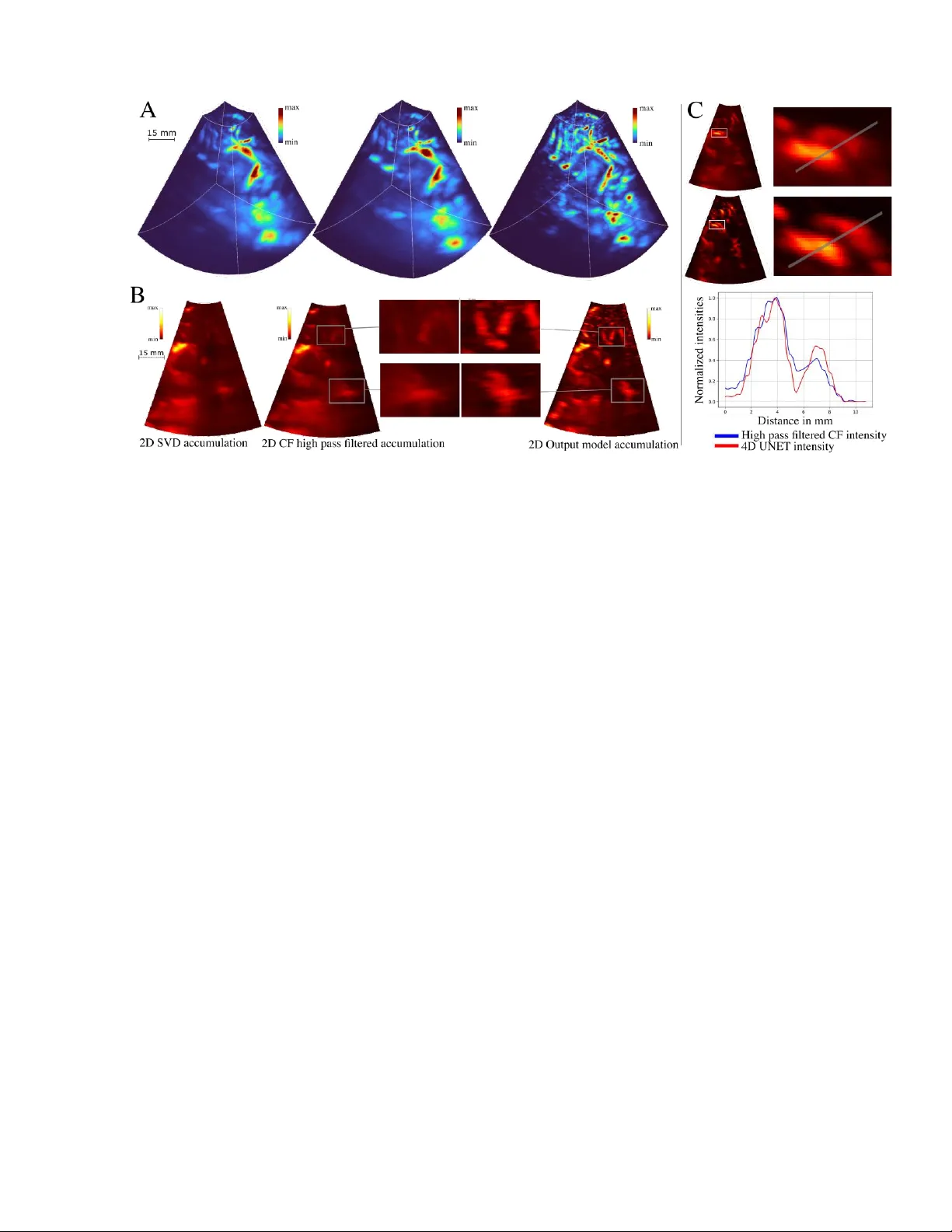
1 Tr istan Beruard, Armand D elbos, Arthur Chavign on, Maxence Reberol , Vincent Hingot Resolve Stroke, Par is, France Abstract Tr anscranial ultrasound imaging is limited by high skull absorption, limiting vascular imaging to only the large st vessels. Traditional clutter filters strugg le with low signal- to -noise ratio (SNR) ultrasound datasets, where blood and tissue signals cannot be easily separated , even when the echoge nicity of the b lood is improved with contrast agents . Here, we pres ent a novel 4D U-N et approach for clutter filtering in transcr anial 3D Contrast Enhanced Ultras ound (CEUS ) exploiting spatial and temporal informati on via a 4D-UNet i mple mentation to en h ance microbubble detection in transcranial data ac quired in human adults . Our result s show that the 4D -UNet improves temporal clutter f ilters. By integrating deep learning in to CEU S, this study advances neurov ascular imaging, offering improved cl utter rejection and visualizat ion. The f indings unders core the potential of AI-driven approaches to enhance ultrasound- based medical imaging, paving the way f or more acc urate diagnostics and broad er clinical applications. 1 INTRODUCTION Brain imaging w ith ultrasound has histor ically been constrained by the high absorption of ultrasound waves through th e skull bone [1] . This challenge is particula rly true when imaging s low blood flows an d small vessels, which are masked by residual clutter caused by background signals originating from the skull and tissues . Moreover, modern microvascular imaging techniques increasingly use unfocused transmit beams to achieve higher frame rates, furth er reducing the signal - to -noi se ratio (SN R). Even in co ntrast enh anced ultraso und (CEUS), where microbubbles (MB) enhance the echogenicity of blood, developing a good clutter filter remains a critical challenge to enable go o d microvascular imaging . Developing a n efficient clut ter rejection filter to highlight the signa l from b lood is a decade old problem w ith n o perfect solutio n [2]. A typical ass umption is that stationary tissues contribute the most to this clutter wh ereas fast moving red blood cells compose the signal to extract. This way, the simplest method to perform clutter rejection is to apply a temp oral filter in the temporal do main [3] . Yet, these filters work o n s hort temporal s equences, limiting their ability to cut low frequencies and to exhibit the slowest flows. To addres s this issue, a new generatio n of filters based on ma trix decomposition of blocs of fra mes using Singular Va lue Deco mposition (SVD) or Pr incipal Component Analysis (PCA) take adva ntage of longer ensemble lengths to improve the sensitivity to slower flows [4]. Alt hough they are often c alled spat io-temporal clutter filters, they are not actu ally sensitive t o s patial patterns within i ndividual fr ames, unlike more recent alg orithms based on machine lear ning. In part icular, Convo lutional Neural Netw orks (CNNs) can r ecognize s patial featur es in complex and n oisy data sets and can furt her increase clutter filter ing in CEUS [5] [6] [7]. In t he context of CEUS , 4D -UNet improves clutter rejection in human transcranial contrast enhanced ultrasound Fig. 1: Complete de composition of the clu tter filtering pipeline, A. RF data, B. High-pas s filter and beamforming , C. 5D slices, D. 3D+t slices, E. 3D+t complete volumes, F. Temp oral accumulation Beruard et al 202 6 2 CNN s can ac t as an addit ional co ntrast a nd reso lution enhancer. The input data for CNNs c an be the raw radiofrequen cy (RF) data [8] , [9] , [10], [17] but most ofte n follows a pre - processing step comprise d of beamforming and c lutter filtering. Th e o utput is ge nerally a map display ing MB concentration or speed and repr esentative of the blood volume or velocity [ 19]. Clutter filters b ased on CNN s rely on a training phase, in which labeled data is fe d into the network. The labe led data originates from either simulated data [20] or the ground truth ca lculated using a regular cl utter f ilter [21] , meaning that those methods cannot be genera lized for dataset w here clutter filters are inefficient. In the hum an brain with unfocused transmit beams, cl utter filters struggle to highlight individual MB and train ing methods are therefore not applicable. In this study, we propose a new way to improve clutter filtering in transcr anial 3D CEUS based on a training paradigm using real microbubbles signa l in water as a training dataset. Additiona lly, we propose to use a 4 D U- N et on 3D+t data to further exploit the spatial and temporal nature of the 3 D CEUS data. This study is performed in a subset of transcranial dat a obtained in human patients with neurovascular alterations and an intact skull. 2 THEORY In o ur implementation, schematized in F igure 1, the model ’s input is a block of preprocess ed data. The input data is a 5D te nsor w here the three first dimensions are the 3D spatial volumes sampl ed by the probe and t he fourth dimension is the evolution of these vo lumes through time . Finally, the last dime nsion corresponds to different “channels” used to trai n the model. The first channel co ntains t he DAS output, t he second channel is the c oherence factor [22] while other channels are the high pass filtered L1 norm of the DAS , and its phase. Then, this 5D tensor is cr opped into small er 5D vol umes measured to fit the spatial expansion of a single MB through time . T hese small 5D cubes are use d as the input of the model. The out put is a 4D volume that is concatenated back t o match the orig inal volume. 2.1 Labe lling strategy and training the model A key limitation of existing implementations of CNN based clutter filterin g is t he generatio n of a lab eled dataset to use as a grou nd trut h for training. In some implementations, individua l MB signals were used as ground truth for further tra ining [13] . In our human clinical dataset, c lassical f ilters do not perform suff iciently w ell to detect micr obubbles wit h a high contrast. Consequen tly, individual MB signal cou ld not be used as a groun d truth for s upervised learning. Therefore, we propose a new training para digm that can be adapted to any in vivo situation without need ing a go od contrast a priori . To achieve th is, we generat e an artificia l grou nd truth from in vitro data as represented in Figure 2. In this approach, two datasets, one of pure clutter, and another of pure MB signal are combined to cre ate the training data. Firs t, an acquisition of MB s in clear water is performed to gen erate a d ataset wi th pure MB signal. T hen, pure clutter sig nal is extracted from real in vivo datasets by selecti ng frames before MB s were injected. Thes e two s ignals are then added together to form the composite dataset. In this composite dataset, the posit ion and intensity of the MBs can be e asily comp uted and serve as ground tr uth. This way, a comprehensiv e pipeline is implemented to train the model w ith a wide number of MB + clutt er configurations, w ith a l oss function based on the input MB signal. Fig. 2: A. (from left to right): Beamfor med MBs in water, beamfor med addition of MBs w ith clutter, ground truth ob tained from the MBs in water / B. Sma ll patches with lef t: C F input of the model, right : Ground truth / C. Example of the trajectory of a MB in a patch Beruard et al 202 6 3 The tr aining d ata is highly specific to t his use case, consequently there is no possibility to use a foundatio nal model [23] , or a pretrained base. The model is therefo re trained from sc ratch. It is s ufficiently small t o be train ed on a local GPU. Inspired b y [24] , we pro pose to tra in t he network using small patches of the data, reduci ng compute-comp lexity and context-depen dency. 2.2 Design of the CN N This input/output c hoice imposes a re gression architecture for t he mo del . Other implementat ions emphasizing the t emporal dimension showed promisi ng results [25 ] . This way, t he MB s ’ pers istence and dynamic s in the spat io-temporal domain can be exploited by the model . Our imple mentation r elies on a 4D U-Net which, to our knowledge, has not been used with CEUS d ata. We did not consi der RN Ns and Tr ansformer based mod els [26], [27], [2 8], as the tempora l informa tion was sufficient ly exploited with a 4- dimensional U-Net arc hitecture. Additionally, t he 4D-U-N et does not introduce any bias favoring the tem poral dimension over s patial dimensio ns or vice versa, as its architecture treats spatial and temporal components in a s tructurally equiva lent manner . U-Nets are pertin ent o ptions for filtering beca use their encoder-decoder architecture effectively isolates background fr om the MBs while r econstructing a cl ean image [24],[29],[30]. Mor e genera lly, com prehensive microvascular imaging implementations based on U-Nets have shown promis ing res ults in animal mod els, where clutter filtering performs better, due t o h igher frequen cy probes, low atten uation a nd controlled imaging con ditions [31] . 3 METHODS The obj ective is to produc e a deep learnin g pipeline to filter out the c lutter and enhance microbubble signal in spatio-temporal sampl es o n ultrasound acquisitions of the brain. There are three ma in points to focus on : acquiring a dataset for tra ining , choosing the model arc hitecture and training the mo del. 3.1 Data acquisition 3.1.1 Clinical data The clinical data was gathered as part of the ESRIR study , reference NCT 06793839 on cl inicaltrials.gov . A s et of 6 anonymized acquisitions were extracted from t he ESRIR study database. Briefly, ultrasound acqu isitions were performe d at 1000 v olumes per second on a 32x32 matrix with a central fr equency of 2 MHz for 165s, representing a total of 16 5000 volumes. For each acquisition, a bolus of 2,4 ml of Sonovue was inject ed after 10s which means th at the first 10 0 00 frames are pure clutter with out MB . A.2 Training data and Ground truth Tr aining data was cr eated by combining datasets of MB signal and of clutt er signal. Pure MB sig nal was acquired in a wate r t ank l ined w ith an absorbent at the bottom. MBs were diluted and s tirred in th e water tank until they visually appeared distinct enoug h on the images, typically separated by 1 cm. A gentle st ir in the water generate d a convection movement which randomized MB trajectories. 8 sets of 3200 frames were acquired with the sam e pro be used to acquire the clin ical data at a frame rate of 100 Hz. This clutter- free data was used to generate training inp uts by adding to it pure clutter. The ground truth was obtained by cropping the easily detectable MBs. Individual MBs wer e identifi ed using th e T rackpy li br ary in Python [32] . The minmass parameter of the Trackpy detection was empirically set by using elbow detect ion on a plot representing the amount of object detected in different frames for mult iple va lues of the minma ss parameter. This method finds a compromise between not labelling noise as a MBs and detec ting as many MBs as possible. The parameters of the detection funct ion w ere a diameter of (5,5,5) and a separation o f (7,7, 7) . The speeds of the b ubbles w ere me asured using Tr ackpy’s linking f unction and were ar ound 1 voxel p er frame . The data was downsam pled to achieve a more divers e distribution of MB speeds, with a un iform spread between 1 voxel/frame and 3 vox el/frame. The linking function from Trackpy was then used again to reconstruct the trajectori es of MBs across multiple frames. To foc us the m odel on learning co nsistent Fig. 3: global archi tecture of the 4D U-Net Beruard et al 202 6 4 trajectories over time, a ny MB trajectori es shorter tha n 2 frames were remov ed from the ground truth . To train the model, p ure Rad io Frequency (RF) MB signals (   ) acquired in water were added t o pure RF clutter signals (   󰇜 from the clinica l study, pri or to beamforming. The rel ative intensity of the MB signa l was modulated to form a uniform dataset us ing a l inear c oefficient  .   served to compu t e the ground truth. We assum ed th at t he ultrasound medium is linear, meaning we neglect ed second order interactions be twe en the clutter and the MBs. 3.2 Pre processing 3.2.1 B.1 Beamforming An initia l step of c lutter filtering was perform ed on the RF data by applying a simple high-pass filter , which removes from each frame the mean of a rolling window of 11 frames . T he deep learning model wi ll serve as a seco nd clutter filtering step. The data used as the inp ut to the model was beamformed to obtain two channels: C oherence Fac tor (CF) and a complex -valued Delay A nd S um ( DAS) . Classical C NN implementations do not acc ept comp lex values , consequently the DAS was split in three channels, one for its am plitude and two for the phase d ifference between the frame    and the frame  :            . T he de phasing is expres sed in rad ians. T o ensure continuity in the tr ansition between  and  and to avo id alias ing, it was split in two separated channels: cos 󰇛  󰇜 and sin 󰇛  󰇜 . Overall, we end ed up with f our input chan nels, CF, DAS amplitude, dephasi ng cosine and dep hasing sin e. 3.2.2 B. 7 Cropping We train ed th e mode l on small s patio-temporal win dows (patches) , to reduce com putational c ost and conte xt dependency. The global output of the model is then given by the reconstruc tion using every small output window . The size of t he patch chosen was 󰇛       󰇜   󰇛       󰇜 , wh ich ensures that most bubble trajec tories stay contained in each patc h since their maximum spe ed is around 3 vox els/frame. 3.2.3 B. 8 Data proc essing We perform ed data augmentation, by ra ndomly swapp ing the spatial axes and r andomly fl ipping the x and y axis. It helped generate more sa mples, with a grea ter variety of directions. Standard normalization was ap plied to the CF and |DAS|. The Dephasing valu es were not norm alized. Normalization by dilation was applied to the grou nd truth, using a morpholog ical dila tion opera tion. This process consists in spat ially expanding the values of t he gro und truth, to em phasize the MBs ’ maximum va lues. A fter dilation, e ach value of th e original ground truth w as divided by its correspo nding dilate d value. T his normalization step enhanc ed the relative intensities and ensur ed that the intensity of the MB’s center is set to 1 . Bubbles on the edg es of th e patches wer e removed from the ground truth so that the model w ould reco gnize complete MBs and ignore cr opped MBs . The i nfer ence on real data is performed using an overl ap between patc hes , which ensures that n o MB will be ignore d. 3.3 Model building 3.3.1 C.1 Model architecture We chose to use the U- N et architecture, introduced in [24] , as the bas is for the filtering net work. The goal of t he filter is to detect th e MBs, which is achieved by se parating them from the tissue. U-N et s have been shown to be ver y proficient in medica l segmentation, m aking them an id eal candidate. The model’s arc hitecture is composed o f three main p arts: the encoder, which extracts features from the input dat a; the bottlenec k, which proc esses these features; and the decoder, which reconstruct s a full -sized 4D output wh ere bubbles are high lighted. Sk ip connect ions are used to concatenate outputs from different encoder l evels to the corresponding decoder levels. These skip connections act as r esidual links, improving rob ust ness to va nishing or exploding gradients [33] and help ing to smooth the l oss landscape [34]. The f inal ac tivation function is a sigmo id from PyTorc h’s implementation since it is widely used in regression tasks and outputs the PSF of a MB normalized be tween 0 and 1. 3.3.2 C.2 Implementation of 4D operators The term 4D refers t o t he fact tha t th e inputs are spatiotemporal. The decision to treat the temporal dimension the same way as the spatial dimensions ste ms from the intu ition that, in 4D, microb ubbles trajectori es f or m tube-like struc tures, which can b e more eff ectively localized by the network. 2 D and 3D U- Nets are wi dely used in research and industrial set tings. They can be directly imp lemented us ing PyTorch, Tensorflow or J ax. However, to our knowle dge no library has imple mented 4- dimensional o perators for c onvolutional networks , th ey are limited to 2D or 3D data . This is why w e built our own 4-dimensional operat ors to process the data. For ba tch normal ization, the 6D tens or X of s ize 󰇟             󰇠 ( batch, channel, space, time) is Beruard et al 202 6 5 reshaped in a 5D one of size 󰇟              󰇠 , which is passed t hrough PyTorch’s  operator . The normalized tensor can the n be res haped t o its orig inal size as the batc h normalization operation preserves element order in PyTorch. With   󰇛 󰇜    󰇛              󰇜 (1) To upsample the te nsor by factors 󰇟      󰇠 , we start by upsampling every 3D slice using Py T orch’s built -in function with a scale factor of 󰇟    󰇠 . We then ad d    copies of the upsamp led sub-tens or between the resulting 3D slices along the fourth d imension, effectively upsampling along this last dimension.      󰇟 󰇛   󰇜  󰇛  󰇜     󰇛  󰇜  󰇛  󰇜󰇠 (2 ) We tack le max pooling by splitting the operation in two. For a pooling of kernel size 󰇟    󰇠 , each spat ial 5D slice of the input is first p assed through PyT orch’s maxp ool3d function w ith a k ernel s ize of 󰇟   󰇠 . This results in a tensor of size 󰇟                󰇠 . We the n a pply the maxpool1d function along the time dimension for ea ch spatial coordi nate with a kernel size of l. This suc cessfully creates the desired output array of size 󰇟                   󰇠 .      󰇛 󰇟  󰇛    󰇜      󰇛   󰇜 󰇠 (3) The im plementation we used for conv olutions w as built and adapted from J an Funke’s git rep ository [33]. The 4D convolution is a genera lization of the 3D convolution. The complete formula with a 4D kernel size of 󰇟      󰇠 and with  the resultin g output is:  󰇛          󰇜                                             (4) With c’ the output chan nel corr esponding, j the position of  in the batch ,   the number of input channels, and 󰇛      󰇜 the positions of the output voxel corresponding to this formula. T he re po si tory’s implementation uses 3D convolution, giving the fo llowing form ula:                      (5) With b th e full tensor of biases ,  the 6D full kernel te nsor and output the 6D f ull output. The    o perator from PyTorch operates over t he c hannels and the b atch dimensions i n addition to t he spatial one. The convolutions use a class ical kernel s ize of 󰇟󰇠 , stride 1 and pad ding ‘ same ’ , both for t he encoder a nd the decoder operations. MaxPooling and UpSampling operations use a w indow of size 󰇟󰇠 . We use d LeakyRelu as activation functions. 3.4 Model training 3.4.1 D.1 Training param eters The loss function c hosen to trai n the model was the mean squared err or, wh ich is a classical c hoice for r egression tasks. The learning rate of the Adam opt imizer was initialized at     , with a weight decay parameter of     . The we ights and b iases were initialized using He initialization. T he learning rate w as carefully Fig. 4: Examples of patches, Left to right: model input, ground truth, model output. A: e xample of the rob ustness of the mode l over spatial de formations on the in put/ B and C: Detection o f two MBs over one pa tch by the model / E: Example of a False Positive output /F: Example of a False negat ive, due to low MB in tensity Beruard et al 202 6 6 scheduled, by firstly s etting i t on constant     , allowing th e mod el to learn the global structure of the MBs trajectories, and th en after X ep ochs when the N eural Network had suff ic iently converged, it was decreas ed using t he Re duceLROnPlateau schedu ler to hel p the model learn the fi ner details of MB tr ajectories. 3.4.2 D.2 Training summary The model was tra ined around 100 epochs, with ea ch epoch taking approxi mately 45 min utes on a Nvidia R TX 4080 with 16 Go o f memory. 4 RESULTS We prese nt results divided into two cat egories: in vitro data, w here the ground truth al lows us to co mpute standard detection metrics; and i n vivo hu man acquisitions, where th e evaluation is qualitative. 4.1 Results over in v itro dataset In the in vitro dataset, t he ground truth is separable from the clutter which a llows us to loca lize MBs. Therefore, it is poss ible to measure the performance of the model f or detection on a test dataset. This test set is compr ised of different acquisitions of MBs that w ere not us ed for training. The metrics used are calculated over the raw model out put . To detect the MBs on the model ’s outputs , the ir centers were detected using a peak detection algorithm from SciPy, by setting an absolute t hreshold adjusted e mpirically, and then fixed for the who le test s et (the peak inte nsity on every frame has to b e greater th an this t hreshold for a spot to be detected as a MB ) . The centers were detected frame by frame and not l inked to form trajectories . T his me ans that one MB trajecto ry contains multip le detected c enters evolving through t ime . The me trics consider only the centers which are at leas t three voxels away fro m the border. Comparing the positions o f M Bs on the mod el o utput to the ground truth, as seen for different situations on t he Figure 4, a llows us to c alculate t he amount of T rue Positive / Fa lse Positive / F alse Negative detections . T he precision, the reca ll and the f1- score are comp uted using these metrics. These scores are depen dent on the i ntensity coefficie nt used to mix th e raw MB data and th e c lutter s ignal. To qu antify this dep endence , the metrics are computed ov er different datase ts with differ ent values for this coef ficient. Each test dataset is c omposed of 3200 s amples (100 batches) extracted from da ta excluded from th e training set. As shown in Figure 5, the scores increase as the inten sity coefficient increases , m eaning th e netw ork det ects MBs more accurately . This is logical as M Bs are best detected when the ratio between their intensity a nd the intensity of clutter is high. At best, the metrics are cappe d between 0. 7 and 0.8 and do not rea c h 1 because som e MBs do not appear in the ground truth, and some groun d truth annotations may not c orrespond to actual M Bs. Additionally, ev en at high intensity , a few MBs remain barely v isible in the tr aining examples, which correspo nd to local areas with h igher clutter noise. The 4D U-Net exhibits limitations when MBs be co me poorly visible: the r ecall score, and conse quently the f1 - score, decrease significantly when the intensity coefficient becomes low. Typically, the threshold used for MB detection over c lutter is in the order of -9 dB [34]. 4.2 Results over in v ivo dataset The model is used on in vi vo human d ata collecte d in a clinical trial. T he compl ete acquisition vo lume is beamformed, obtaining all input channels. A h igh p ass filtering operation is performed on the data bef ore the beamforming and standardization is applied, exactly li ke on the training data. The t emporal volume is divided in 4D patches with a spatial overlap of 6 voxels between adjacent p atches. To avoid a higher intensity on the border of output patches due to the summed overlap , voxel v alues on the borders are combined using Ga ussian weights center ed on ea ch patch. The m odel’s outputs for every patch are reassembled into a co mplete volume. The high pass fil t ering + 4D U-Net metho d is compared to h igh pass filtered CF ac cumulation, a nd S VD filter ed CF accumulation. The SVD is done by cutting off th e 20 first eigenval ues of the temporal dimens ion over blocks of 256 frames. Figure 6 shows that the 4D-U -Net isolates MBs signal from the backgr ound better t han SVD or high pass filtering. Fig. 5: Score s of the 4D U-Net depending on the intensity coefficient that w eigh ts the MBs in the sum Tissue + MBs (log scale) Beruard et al 202 6 7 Results are accumu lated o ver 6400 acquis ition fra mes, corresponding to 6,4s of acquisit ions, along t heir corresponding frame indices . Specifically, f or each frame position within a block, the res ulting b lock contains t he sum of all fra mes at the sam e position across th e previo us blocks. Finally, the standard deviation is compute d for e ach voxel in the resulting block, enhancing the visib ility of MBs trajectories. T he se t emporal accumulation s can be s een on Figure 7. The v essels appear thinner in the model output, leading to better vessel separat ion compare d to SVD and high pass filtering alone ( Figure 7.C) . Additionally, c ertain vas cular s tructures are more c learly visible ( Figure 7. C) i n th e model output than in the classical results, highligh ting the model ’s high sensitivity. 5 D ISCUSSION The vascularization that is visible in the accumulatio ns with high-pass filter and SVD filter can be improved by t he model. T his can be observed on the accumulat ions, and in s ome regions a better separation of the v essels is noticeable. A hypothes is to expl ain the be havior of t he model is that t he improve ment possibly orig inates fr om the s hape of the mod el's output, which contain s maller bubble t han in t he filtered data, which also ha ve a w ider and more unifor m s pherical shape. Th is wou ld b e a PSF thinning behav ior. Furthermore, certain vascular structures that are bare ly discernible after high-pass filtering a ppear more clearly in the model, indicating the model's higher sensitivity to certain MBs that are faintly visible but are seem ingly pulled out fro m the noise by the model. T his incre ase in sensitivity can be attrib uted to the mode l’s improv ed recognition of characterist ic spatial patterns of M Bs a nd its robustness to tempora l signal interruptions, which are common in in vivo data. The model enforc es s patial patterns t hat are temporally propagated , like a MB moving , and can outperfor m temp oral f ilters when MBs flicker or momentari ly disappear. T he indiv idual spatial patterns of MBs are not considered in the SVD, which performs purely temporal filtering , a lbeit o n proj ected singular spatia l vectors, but without highlighting special spatial structures. A limitation is that t he model’s accumu lation appears more discontinuous than the acc umulations of th e h igh pass filtered, a nd n ot compounding th e di ffuse s ignal of undetected MBs wh ich s till contributes to the over all signal. This c reates a sharper image, where only structures with s trong MBs signal c an be s een. This is advantageous for morph ological me asurements, but can be de trimental to perfus ion or functiona l imaging, whe re the temporal changes of t he backgrou nd s ignal c an be indicative of physiolog ical changes. Although all t he data wer e acquired w ith the same probe and system , the d eformations present in real i n vi vo data are n ot p erfectly r eproduced in the i n vitro data used f or training the model, as the MBs-tissue interac tions were not modeled and thus negl ected. Th e PSF of in vivo MB is therefore different fr om that of in vitro MBs, as the wavefront undergoes significant dist o rt ion d uring pr opagation through the tissue and while passing throu gh the skull. This highlights a clear avenue f or improving our method, which could involve the use of labeled in vivo data. One pot ential approach to enhance labeling co uld be l everaging the c urrent 4D-UN et to prov ide an initial estimation of the MBs ’ positions, thereby faci litating manual labeling. The model captures tempor al coherence over a maximum of only 8 frames w hereas SVD levera ges long tempo ral windows to extract clutter characteristics . One potent ial improvement for the 4D-UNet model w ould be to increase the size of the temporal window to incorporate a broader temporal context. Additionally , the model’s input data is already filter ed, which reduces the inform ation available to th e model compared to unfiltered data. Another possible enhancement wo uld be to decrease the c ut off freque ncy of the h igh pass filter applied to the m odel ’s input, allow ing it to exp loit a larger i nformation source . This partly explains why only MBs with in large brain vasc ulature ar e Fig. 6: Compari son of a temporal fr ame of 3D volumes (MIP view) between differen t filters steps. The three first volumes (in the order top left, top righ t, down left) are ov er the CF only Beruard et al 202 6 8 visible, as t hey exhibit sufficiently fast dyna mics to s tay visible aft er the high-pass filter. Convers ely, small brain vessels contain s low-moving MBs whose information is lost to the high -pass fi lter. Reducing the intens ity of this filter while i ncreasing the t emporal window could al low the recovery of new trajectories within smaller vascular structures. Unfortunately, increasing the size of the temp oral windows would require t he use of different deep learning architectures, capa ble of handling long temporal dependencies, such as transformers. 6 REFERENCES G. Pinton, J.-F. Aubry, E. Bossy, M. Muller, M. Pernot, et M. Tanter, « Attenuation, scattering, and absorption of ultrasound in the skull bone », Med. Phys. , vol. 39, n o 1, p. 299  307, janv. 2012, doi: 10.1118/1.3668316. [2] S. Bja erum, H. Torp, et K. Kristoffersen, « Clutter filter design for ultrasound color flow imagi ng », IEEE Trans. Ultrason. Ferroelectr. Freq. Control , vol. 49, n o 2, p. 204  216, févr. 2002, doi: 10.1109/58.985705. [3] C. Ty soe et D. H. Evans, « Bias in mean frequency e stima tion of Doppler signa ls due to wall clutter fi lte rs » , Ultrasound Med. Biol. , vol. 21, n o 5, p. 671  677, janv. 1995, doi: 10.1016/0301-5629(95)00009- G. [4] C. Dem ené et al. , « Spatiotemporal Clutter Filtering of Ultrafa st Ult rasound Data Highl y I ncreases Doppler and fUltrasound Sensitivity », IEEE Trans. Med. Imaging , vol. 34, n o 11, p. 2271  2285, nov. 2015, doi: 10.1109/TMI.2015.2428634. [5] O. Russ akovsky et al. , « Imag eNet L arge Scale Visual Recognition Challenge », 30 janvier 2015, arXiv 10.48550/arXiv.1409.0575. [6] A. Kri zhevsky, I. Sutskever, et G. E. Hinto n, « ImageNet Classification with Deep Convolutional Neural Networks », in Advances in Neural Information Processing Systems , Curran Associates, Inc., 2012. Consulté le: 13 janvier 2025. [En ligne]. Disponible sur: https://proceedings.neurips.cc/paper_files/pa per/2 012/hash/c399862d3b9d6b76c8436e924a68c 45b - Abstract.html [7] K. He, X. Zhang, S. Ren, et J. Sun, « Delving Deep into Rectifiers: Surpassing Human-Level Performance on ImageNet Classification », in 2015 IEEE International Conference on Computer Vision (ICCV) , déc. 2015, p. 1026  1034. doi: 10.1109/ICCV.2015.123. [8] A. C. L uchies et B. C. Byram, « Deep Neural Networks for Ultrasound Beamforming », IEEE Trans. Med. Imaging , vol. 37, n o 9, p. 2010  2021, sept. 2018, doi: 10.1109/TMI.2018.2809641. Fig. 7: (A): 3D temporal accumulat ions, from Left to right: SVD filtered and CF bea mformed data, High pass filtered and CF beamformed data, 4D UNET output o ver CF and DAS high pass filtered data. (B): 2D slice of temporal a ccumulation (C): Zoo m over two va scularization and comparison of the spatial separa tion over the dra wn segment between High pass filtered CF and 4D UNET output ove r CF and DAS high pass f ilt ered d ata. Beruard et al 202 6 9 [9] D. Hyu n, L. L. Brickson, K. T. Loo by, et J. J. Dahl, « Beamforming and Speckle Reduction Using Neural Networks », IEEE Trans. Ultrason. Ferroelectr. Freq. Control , vol. 66, n o 5, p. 898  910, mai 2019, doi: 10.1109/TUFFC.2019.2903795. [10] W. Gu, B. Li, J. Luo, Z. Yan, D. Ta, et X. Liu, « Ultrafast Ultrasound Localization Microscopy by Conditional Generative Adversarial Network », IEEE Trans. Ultrason. Ferroelectr. Freq. Control , vol. 70, n o 1, p. 25  40, janv. 2023, doi: 10.1109/TUFFC.2022.3222534. [11] K. G. Brown, D. Ghosh, et K. Hoyt, « Deep Learning of Spat iotemporal Filtering for Fast Super -Resolution Ultrasound Imaging », IEEE Trans. Ultrason. Ferroelectr. Freq. Control , vol. 67, n o 9, p. 1820  1829, sept. 2020, doi: 10.1109/TUFFC.2020.2988164. [12] « Deep Learning-Based Microbubble Localization for Ultrasound Localization Microscopy | IEEE Jo urnals & Magazine | I EEE Xplore ». Consulté le: 13 janvier 2025. [En ligne]. Disponible sur: https://ieeexplore.ieee.org/document/9715054 [13] Y. Shin et al. , « Context-aware deep learning enables high-efficacy localization of high concentration microbubbles for super- resolution ultrasound localization microscopy », Nat. Commun. , vol. 15, n o 1, p. 2932, avr. 2024, doi: 10.1038/s41467- 024 - 47154 - 2. [14] X. Liu, T. Zhou, M. Lu, Y. Yang, Q. He, et J. Luo, « Deep Learning for Ultrasound Localization Microscopy », IEEE Trans. Med. Imaging , vol. 39, n o 10, p. 3064  3078, oct. 2020, doi: 10.1109/TMI.2020.2986781. [15] G. Zhang et al. , « ULM-MbCNRT: In vivo Ultrafast Ultrasound Localization Microscopy by Combining Multi-branch CNN and Recursive Transformer », IEEE Trans. Ultrason. Ferroelectr. Freq. Control , vol. PP, avr. 2024, doi: 10.1109/TUFFC.2024.3388102. [16] L. Milecki et al. , « A Deep Learning Framework for Spatiotemporal Ultrasound Localization Microscopy » , IEEE Trans. Med. Imaging , vol. 40, n o 5, p. 1428  1437, mai 2021, doi: 10.1109/TMI.2021.3056951. [17] Z. Zhang, M. Hwang, T. J. Kilbaugh, et J. Katz, « Improving sub-pixel accuracy in ultrasound localization microscopy using supervised and self-supervised deep learning », Meas. Sci. Technol. , vol. 35, n o 4, p. 045701, janv. 2024, doi: 10.1088/1361- 6501/ad1671. [18] N. Blanken, J. M. Wolterink, H. Delingette, C. Brune, M. Versluis, et G. Lajoinie, « Super-Resolved Microbubble Localization in Single-Channel Ultrasound RF Signals Using Deep Learning » , IEEE Trans. Med. Imaging , vol. 41, n o 9, p. 2532  2542, sept. 2022, doi: 10.1109/TMI.2022.3166443. [19] Y. Zhang et al. , « Efficient Microbubble Trajectory Tracking in Ultrasound Localization Microscopy Using a Gated Recurrent Unit-Based Multitasking Temporal Neural Network », IEEE Trans. Ultrason. Ferroelectr. Freq. Control , vol. 71, n o 12: Breaking the Resolution Barrier in Ultrasound, p. 1714  1734, déc. 2024, doi: 10.1109/TUFFC.2024.3424955. [20] W. Gu, Z. Yan, B. Li, C. Liu, D. Ta, et X. Liu, « GAN-Based Ultrasound Localization Microscopy », in 2022 IEEE International Ultrasonics Symposium (IUS) , oct. 2022, p. 1  4. doi: 10.1109/IUS54386.2022.9957520. [21] W. Han, Y. Zhang, Y. Zhao, A. Luo, et B. Peng, « 3D U-Net3+ Based Microbubble Filtering for Ultrasound Localization Microscopy », in 2023 IEEE International Conference on Systems, Man, and Cybernetics (SMC) , oct. 2023 , p. 3974  3979. doi : 10.1109/SMC53992.2023.10394576. [22] R. Mallart et M. Fink, « Adaptive focusing in scattering media through sound-speed inhomogen eities: The van Cittert Zer nik e approach and focusing criterion », J. Acoust. Soc. Am. , vol. 96, n o 6, p. 3721  3732, déc. 1994, doi: 10.1121/1.410562. [23] J. Ma, Y. He, F. Li, L. Han, C. You, et B. Wang, « Segment anything in medical images », Nat. Commun. , vol. 15, n o 1, p. 654, janv. 2024, doi: 10.1038/s41467-024-44824- z. [24] O. Ronneberger, P. Fischer, et T. Brox, « U-Net: Convolutional Networks for Biomedical Image Segmentation », 18 mai 2015, arXiv [25] V. Pustovalov, D. H. Pham, et D. Kouamé, « Enhanced Localization in Ultrafast Ultrasound Imaging Through Spatio - Temporal Deep Learning », in 2024 32nd European Signal Processing Conference (EUSIPCO) , août 2024, p. 780  784. doi: 10.23919/EUSIPCO63174.2024.10715395. [26] A. Dosovitskiy et al. , « An Image is Worth 16x16 Words: Transformers for Image Recognition at Scale », 3 juin 2021, arXiv : [27] F. A. Gers, J. Schmidhuber, et F. Cummins, « Learning to forget: continual prediction with LSTM », Neural Comput. , vol. 12, n o 10, p. 2451  2471, oct. 2000, doi: 10.1162/089976600300015015. [28] A. Vaswani et al. , « Attention Is All You Need », 2 août 2023, arXiv [29] R. Couturier, G. Perrot, et M. Salomon, « Image Denoising Usin g a Deep Encoder-Decoder Network with Skip Connections », in Lecture Notes in Computer Science (LNCS) , in Lecture Notes in Computer Science (LNCS), vol. 11306. Beruard et al 202 6 10 Siem Reap, Cambodia: Springer, déc. 2018, p. 554  565. Consulté le: 13 janvier 2025. [En ligne]. Disponible sur: https://hal.science/hal-02182820 [30] F. Milletari, N. Navab, et S.-A. Ahmadi, « V-Net: Full y Co nvolutional Neural Networks for Vo lum etric Medical Image Segmentation », 15 juin 2016, arXiv [31] G. Zhang et al. , « In vivo ultrasound localization microscopy for high-density microbubbles », Ultrasonics , vol. 143, p. 107410, sept. 2024, doi: 10.1016/j.ultras.2024.107410. [32] « Trackpy: Fast, Flexible Particle-Tracking Toolkit — trackpy 0.6.4 documentation » . Consulté le: 3 mars 2025. [En ligne]. Disponible sur: https://soft-matter.github.io/trackpy/v0.6.4/ [33] T. Gebhard, timothygebhard/pytorch-conv4d . (18 février 202 4). Python. Consulté le: 13 janvier 2025. [En ligne]. Disponible sur: https://github.com/timothygebhard/pytorch-conv4d [34] A. Chavignon, B. Heiles, V. Hingot, C. Orset, D. Vivien, et O. Couture, « 3D Transcranial Ultrasound Localization Microscopy in the Rat Brain With a Multiplexed Matrix Probe », IEEE Trans. Biomed. Eng. , vol. 69, n o 7, p. 2132  2142, juill. 2022, doi: 10.1109/TBME.2021.3137265.