The Geometry of Noise: Why Diffusion Models Don't Need Noise Conditioning

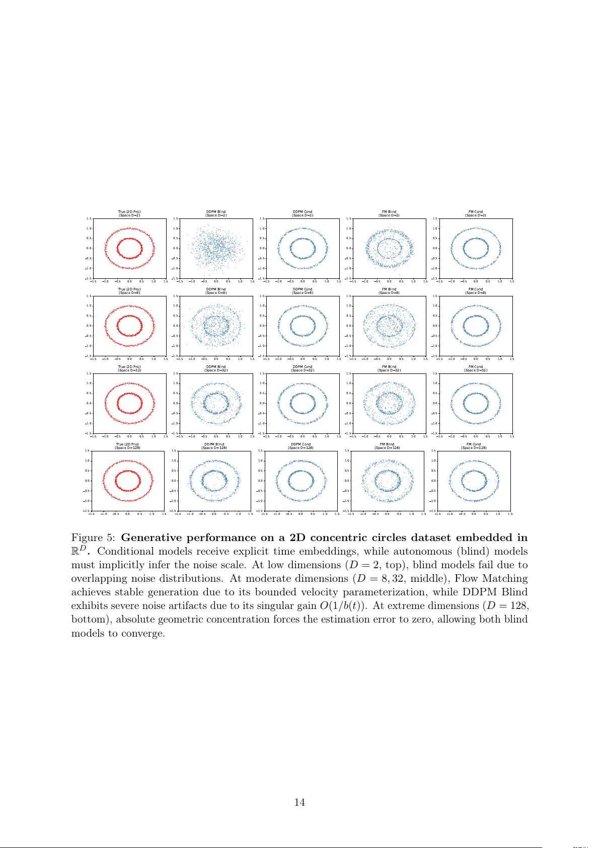
The Geometry of Noise: Wh y Diffusion Mo dels Don’t Need Noise Conditioning Mo jtaba Sahraee-Ardak an, Mauricio Delbracio, P eyman Milanfar Go ogle Abstract Autonomous (noise-agnostic) generativ e mo dels, suc h as Equilibrium Matching and blind diffusion, c hallenge the standard paradigm by learning a single, time-inv arian t vector field that operates without explicit noise-level conditioning. While recen t work suggests that high-dimensional concentration allows these mo dels to implicitly estimate noise lev els from corrupted observ ations, a fundamen tal paradox remains: what is the underlying landscap e b eing optimized when the noise level is treated as a random v ariable, and how can a b ounded, noise-agnostic net work remain stable near the data manifold where gradien ts t ypically diverge? W e resolve this parado x b y formalizing Marginal Energy , E marg ( u ) = − log p ( u ) , where p ( u ) = R p ( u | t ) p ( t ) dt is the marginal densit y of the noisy data in tegrated ov er a prior distribution of unkno wn noise levels. W e prov e that generation using autonomous mo dels is not merely blind denoising, but a sp ecific form of Riemannian gradient flow on this Marginal Energy . Through a nov el relativ e energy decomp osition, we demonstrate that while the raw Marginal Energy landscap e possesses a 1 /t p singularit y normal to the data manifold, the learned time-in v ariant field implicitly incorp orates a lo cal conformal metric that p erfectly coun teracts the geometric singularity , conv erting an infinitely deep p oten tial well into a stable attractor. W e also establish the structural stability conditions for sampling with autonomous mo dels. W e iden tify a “Jensen Gap” in noise-prediction parameterizations that acts as a high-gain amplifier for estimation errors, explaining the catastrophic failure observ ed in deterministic blind models. Con versely , we prov e that v elo cit y-based parameterizations are inherently stable b ecause they satisfy a b ounded-gain condition that absorbs p osterior uncertaint y into a smooth geometric drift. 1 In tro duction Generativ e mo deling has seen immense progress ov er the past decade, tracing its ro ots to the foundational non-equilibrium thermo dynamics approac h introduced b y [ 26 ]. This paradigm was p opularized and scaled by Denoising Diffusion Probabilistic Mo dels (DDPM) [ 13 ] and subsequent arc hitectural refinemen ts [ 5 ], Score-based mo dels [ 27 , 28 , 32 ], and subsequently unified under the con tinuous-time mathematical framework of score-based sto c hastic differen tial equations (SDEs)[ 29 ]. F or a broader conceptual ov erview of ho w these p ersp ectiv es on diffusion hav e evolv ed, see [ 6 , 10 ]. More recently , the field has ev olved b ey ond pure diffusion to em brace v elo cit y-based transp ort form ulations [ 1 , 4 , 21 ], notably Flow Matc hing [ 20 ], as well as stationary targets like Equilibrium Matching (EqM)[ 33 ]. A defining characteristic of these standard generative mo dels is their reliance on explicit time-conditioning. They t ypically learn a conditional score function or v elo cit y field, suc h as ϵ θ ( u , t ) , defining a dynamic field that changes with time, i.e. a field ov er R D × [0 , 1] . In these framew orks, the netw ork relies on the time v ariable t to dictate the current scale of corruption and orient the tra jectory . In contrast, recent work has explored autonomous approaches, such as EqM [ 33 ] or noise-blind diffusion [ 15 , 28 , 30 ], whic h learn a single noise-agnostic vector field f θ ( u ) independent of t . W e 1 denote the optimal vector field learned b y suc h a mo del as f ∗ ( u ) . It is imp ortan t to distinguish the model’s architecture from the resulting inference dynamics: while the sampling pro cess may still utilize a time-dep endent sc hedule to scale the tra jectory , the underlying neural net work is strictly time-inv ariant. This autonomous approac h presen ts a fundamen tal puzzle: the “correct” gradien t to follo w from a p oin t u should dep end heavily on its noise level. Ho w can a single, static v ector field effectively guide a sample from pure noise (high t ) and also guide a sample from ligh t noise (lo w t ), all while ensuring its stationary p oin ts accurately reflect the clean data X ? In this pap er, we resolve this parado x. W e sho w that such an autonomous mo del is not merely acting as a “blind” denoiser, but is implicitly learning a h ybrid field that is fundamen tally tied to a single, non-parametric marginal energy landscap e ( E marg ). This energy is defined as the negativ e log-likelihoo d of the marginal data distribution p ( u ) = R p ( u | t ) p ( t ) dt : E marg ( u ) = − log  Z p ( u | t ) p ( t ) dt  . (1) W e build our argument as follows: 1. The Energy Parado x: W e define the marginal energy and derive its explicit gradient. W e rigorously show that this gradien t diverges near the data manifold, creating an infinitely deep p otential w ell that forbids stable gradient descent. 2. Energy-Aligned Decomp osition: W e analyze the learned autonomous v ector fields, pro ving they decomp ose into exactly three geometric comp onen ts: a natural gradient, a transp ort correction (co v ariance) term, and a linear drift. 3. Riemannian Gradient Flo w: W e resolv e the singularity paradox by showing that noise- agnostic mo dels implicitly implement a Riemannian gradient flow. The learned vector field incorp orates a lo cal conformal metric (the effective gain) that p erfectly preconditions and coun teracts the geometric singularity of the ra w energy landscap e. 4. Stabilit y of Sampling with Autonomous Mo dels: W e establish the mathematical conditions necessary for sampling stability . W e pro ve that velocity-based parameterizations (e.g., Flow Matching, EqM) succeed b ecause they absorb p osterior uncertaint y into a stable drift, whereas standard noise-prediction parameterizations (e.g., DDPM/DDIM) act as high-gain amplifiers for estimation errors, leading to structural instabilit y . 2 Related W ork Our w ork unifies and grounds three recen t lines of inquiry in generativ e mo deling: noise uncondi- tional generation, equilibrium dynamics, and energy-based training. Noise-Blind Denoising. The prev ailing paradigm in score-based mo deling relies on condi- tioning the net work on the noise lev el t [ 27 ]. How ev er, Sun et al. [ 30 ] recen tly challenged this, demonstrating that “blind” models can ac hieve high-fidelity generation without t . This connects to earlier findings in image restoration b y Gnanasam bandam and Chan [ 11 ] , who show ed that a single “one-size-fits-all” denoiser could appro ximate an ensem ble of noise-sp ecific estimators. Our w ork pro vides the rigorous theoretical justification for these observ ations, identifying E marg as the implicit ob jective and connecting the gradients of this energy to the autonomous fields via concen tration of the noise level given the noisy signal. In concurren t work, Kadkho daie et al. [ 15 ] pro vide a highly rigorous statistical analysis of blind denoising diffusion mo dels (BDDMs) for data with lo w intrinsic dimensionalit y . They analytically prov e that under the assumption that the intrin sic dimension is muc h smaller than the ambien t dimension ( k ≪ d ), BDDMs can accurately estimate the true noise lev el from 2 a single observ ation and implicitly track a v alid noise schedule, providing robust finite-time sampling guaran tees. While their w ork offers an exhaustiv e and rigorous statistical treatmen t of this low-dimensional data regime, our w ork situates this concentration of measure as a sp ecific asymptotic case (Regime I) within a broader geometric framew ork. Sp ecifically , our fo cus lies in connecting noise-blind generation to the gradient of the marginal energy landscap e, revealing the pro cess as a Riemannian gradien t flow. F urthermore, whereas their analysis fo cuses primarily on sp ecific Langevin-type SDE discretizations, our framew ork is generalized across arbitrary affine diffusion pro cesses and learning targets. Finally , while they demonstrate that blind denoisers can outp erform non-blind counterparts by a voiding schedule mismatc h errors, our framework allo ws us to prov e why mo dels trained to predict noise (e.g., DDPM/DDIM) are structurally unstable for autonomous generation due to gradien t singularities, demonstrating why velocity- or signal-based targets are strictly necessary . Energy Landscap es & Singularities. While the framework of energy-based learning is w ell-established [ 7 , 17 ], explicitly learning energy functions is kno wn to be unstable [ 8 ]. Recen t approac hes lik e “Dual Score Matching” [ 12 ] attempt to stabilize this b y learning a joint energy via b oth space and time scores. Our work analyzes the mar ginal energy , aligning with Scarvelis et al. [ 25 ] , who pro ved that the exact closed-form score of a finite dataset degenerates in to a nearest-neigh b or lo okup. While they address this b y smo othing the score kernel, w e show that autonomous flow mo dels resolv e it implicitly via a Riemannian preconditioner. Equilibrium Dynamics & Flo w. W ang and Du [ 33 ] in tro duced Equilibrium Matching (EqM) to replace time-dep enden t fields with a single time-inv ariant gradient. This parallels Action Matc hing [ 22 ]. Our analysis reveals that EqM is unique: it implemen ts a natural gradient descent on the marginal energy . This connects EqM to the fundamen tal JKO scheme [ 14 ], unifying “transp ort” and “restoration” under a single autonomous field. 3 Preliminaries: A Unified Sc hedule F orm ulation T o pro vide a general theory co vering Diffusion Mo dels (DDPM, EDM) and Flow Matc hing (EqM), w e adopt the unified affine formulatio n prop osed by Sun et al. [ 30 ]. Let t ∈ [0 , 1] index the noise level. The noisy observ ation u t is constructed from clean data x and noise ϵ ∼ N ( 0 , I ) via metho d-specific schedule functions a ( t ) and b ( t ) : u t = a ( t ) x + b ( t ) ϵ . (2) Assuming that the data is normalized, the signal-to-noise ratio (SNR) at time t is SNR = a 2 ( t ) b 2 ( t ) . (3) Generativ e models are typically trained to predict a linear target r ( x , ϵ , t ) = c ( t ) x + d ( t ) ϵ b y minimizing the Mean Squared Error (MSE): L ( f ) = E x , ϵ ,t  ∥ f ( u t ) − ( c ( t ) x + d ( t ) ϵ ) ∥ 2  . (4) In the standard diffusion paradigm, f is explicitly conditioned on the noise lev el t , i.e. it has the form 1 f t ( u ) . The minimizer of the MSE loss is then the conditional exp ectation of the target: f ∗ t ( u ) = E x , ϵ | u ,t [ c ( t ) x + d ( t ) ϵ ] . (5) 1 While a more accurate notation would ha ve been f ( u , t ) , with some abuse of notation we use f t ( u ) to denote a function of u and t to keep the notation consistent with the autonomous mo dels. 3 T able 1: Unified co efficien ts and simplification of the general autonomous field for common generativ e mo dels: DDPM [ 13 ], EDM [ 16 ], Flo w Matching (FM) [ 20 ], and Equilibrium Matc hing (EqM) [ 33 ]. Mo del a ( t ) b ( t ) c ( t ) d ( t ) Autonomous field f ∗ ( u ) = E t | u [ f ∗ t ( u )] DDPM √ ¯ α t √ 1 − ¯ α t 0 1 E t | u h u − √ α t D ∗ t ( u ) √ 1 − α t i = E t | u [ ϵ ∗ t ( u )] EDM 1 σ t 1 0 E t | u [ D ∗ t ( u )] FM 1 − t t − 1 1 E t | u h u − D ∗ t ( u ) t i EqM 1 − t t − t t E t | u [ u − D ∗ t ( u )] This function defines a time-dep enden t vector field that guides the generation pro cess. In this work, ho wev er, we fo cus on autonomous mo dels where the netw ork f ( u ) receives only the noisy observ ation u , with no access to t . The minimizer of the MSE loss for such a “noise-agnostic” mo del is the p osterior exp e ctation of the target (Lemma 1 in Appendix A.1 ): f ∗ ( u ) = E t | u  E x , ϵ | u ,t [ c ( t ) x + d ( t ) ϵ ]  = E t | u [ f ∗ t ( u )] . (6) This has a very in tuitive interpretation: the optimal autonomous mo del is a time-aver age of the optimal c onditional mo del with r esp e ct to the p osterior p ( t | u ) . By defining the optimal conditional denoiser as D ∗ t ( u ) = E [ x | u , t ] , w e can expand this target as (Lemma 2 in App endix A.1 ): f ∗ ( u ) = E t | u  d ( t ) b ( t ) u +  c ( t ) − d ( t ) a ( t ) b ( t )  D ∗ t ( u )  . (7) Sp ecific choices for the co efficien ts a ( t ) , b ( t ) , c ( t ) , d ( t ) yield standard architectures, as summarized in T able 1 . In the table, DDPM form ulation uses the so called v ariance preserving diffusion pro cesses where co efficien ts a ( t ) and b ( t ) satisfy a 2 ( t ) + b 2 ( t ) = 1 and a ( t ) = √ ¯ α t is defined via a discrete diffusion pro cess that determine the form of ¯ α t [ 13 , 23 ]. The c entr al question of this p ap er is to understand the ge ometric and dynamic al c onse quenc es of r eplacing the pr e cise c onditional field f ∗ t ( u ) with this autonomous p osterior aver age f ∗ ( u ) . Do es this time-invariant field stil l define a valid gener ative tr aje ctory? In the following sections, we analyze its alignmen t with an energy landscap e (Section 4 ) and deep dive into its prop erties when used as a generative mo del (Sections 5 and 6 ). 4 The Geometry of the Marginal Energy Standard diffusion mo dels rely on a time-dep enden t score function, ∇ u log p ( u | t ) , which explicitly guides the tra jectory at every noise lev el. In con trast, autonomous mo dels (such as Equilibrium Matc hing or “blind” diffusion) must compress these dynamics in to a single, static vector field f ∗ ( u ) that is indep enden t of time. This fundamental difference raises a critical geometric question: Do es this static field align with the gr adient of a glob al p otential ener gy? If suc h a p oten tial exists, autonomous generation could b e theoretically grounded as a form of energy minimization [ 17 ]. 4 The most natural candidate for this p oten tial is the mar ginal ener gy E marg ( u ) , defined as the negativ e log-likelihoo d of the marginal data density p ( u ) = R p ( u | t ) p ( t ) dt : E marg ( u ) = − log p ( u ) . (8) T o determine if the learned field f ∗ ( u ) aligns with this energy , w e m ust first deriv e its gradient. By differen tiating the marginal lik eliho od mixture, we find that the gradient of the marginal energy is the p osterior exp ectation of the conditional scores: ∇ u E marg ( u ) = E t | u [ −∇ u log p ( u | t )] . (9) W e refer the reader to Lemma 3 for the pro of. T o ev aluate this expectation, we use T weedie’s form ula [ 9 , 24 ] to express the conditional score in terms of the optimal denoiser: ∇ u log p ( u | t ) = a ( t ) D ∗ t ( u ) − u b ( t ) 2 . (10) Substituting this directly into the p osterior exp ectation yields the explicit form of the marginal energy gradient: ∇ u E marg ( u ) = E t | u  u − a ( t ) D ∗ t ( u ) b ( t ) 2  . (11) This result establishes the link betw een the static geometry and the dynamic denoising pro cess. Ho wev er, it also exp oses a critical fla w in the landscap e itself. 4.1 The Energy P aradox A k ey requiremen t for generativ e mo deling is that the learned v ector field f ∗ ( u ) m ust b e consistent with the clean data supp ort. Dep ending on the sp ecific form ulation, the field at the b oundary ( t → 0 ) generally b eha ves in one of tw o wa ys: Case 1: A ttractors (EqM, EDM). F or equilibrium-based mo dels, the target is the data itself or a restoration term. Here, the ideal field m ust v anish at the clean data ( f ∗ ( x ) = 0 ) to create a stable fixed p oin t. Case 2: T ransv ersal Flo ws (Flow Matc hing). F or transp ort-based models, the target is a v elo cit y v ector (e.g., x 1 − x 0 ). A t the data, the field do es not v anish but con verges to a finite, non-zero v elo cit y ve ctor ( f ∗ ( x ) ≈ 0 − x ) that ensures the tra jectory in tersects the data manifold at the correct time. The Singularit y . Regardless of whether the field acts as an attractor or a transversal flow, the mo del faces a ge ometric singularity . As established in App endix B , the p osterior p ( t | u ) collapses near the data manifold. The term inside the exp ectation in Equation ( 11 ) has a singularit y as t → 0 . Consequen tly , the marginal energy forms an infinitely deep p oten tial w ell ( E marg → −∞ , see F igure 1 ), causing the asso ciated gradient field to div erge: lim u → x k ∥∇ u E marg ( u ) ∥ = ∞ . (12) This creates a puzzle: how can a neural net work learn a b ounded vector field (which must be finite at the data) that aligns with a geometry defined by such a singular p otential? One migh t argue that in practice, training is stabilized b y truncating the noise level at some t min > 0 (the “ill-conditioned regime”). Ho wev er, this do es not resolve the geometric parado x; it merely con verts a mathematical singularit y into an extremely stiff optimization landscap e where 5 1.00 0.75 0.50 0.25 0.00 0.25 0.50 0.75 1.00 u 1 1.00 0.75 0.50 0.25 0.00 0.25 0.50 0.75 1.00 u 2 3 2 1 0 1 2 3 4 3D Ener gy Landscape 1.00 0.75 0.50 0.25 0.00 0.25 0.50 0.75 1.00 u 1 1.00 0.75 0.50 0.25 0.00 0.25 0.50 0.75 1.00 u 2 Contour V iew Data Manifold 2.25 1.50 0.75 0.00 0.75 1.50 2.25 3.00 3.75 E n e r g y l o g p ( u ) Figure 1: The Singular Geometry of the Marginal Energy Landscap e. (Left) 3D Energy Landscap e: A visualization of the marginal energy E marg ( u ) = − log p ( u ) . The landscap e reveals an infinitely deep p otential well at the data manifold, where the energy diverges to −∞ . (Righ t) Con tour View: T op-do wn p erspective sho wing the energy concen tration around discrete data p oin ts (stars). While the raw gradient ∇ u E marg ( u ) b ecomes singular as u approac hes the clean data, in this w ork w e pro ve that autonomous mo dels remain stable b y implicitly implementing a Riemannian gradient flow. In this framework, the p osterior noise v ariance acts as a lo cal conformal metric that preconditions and p erfectly coun teracts the geometric singularity . Hessian eigenv alues scale as 1 /t 2 min . Whether strictly singular or merely ill-conditioned, the ra w energy landscap e essen tially forbids stable gradient descent. In the next section, we resolve this puzzle by showing that noise-blind mo dels do not follo w the ra w energy gradient, but rather a R iemannian gr adient flow that p erfectly preconditions this singularit y . 5 Autonomous Generation as Riemannian Gradien t Flo w W e resolv e the parado x of stable con vergence d espite divergen t gradients by showing that autonomous models implement a Riemannian gradient flow. W e sho w that the learned v ector field f ∗ ( u ) is structurally identical to the natural gradient of the marginal energy , but with a critical correction term that dominates only when geometric concen tration fails. 5.1 The Anatom y of the Autonomous Field Recall from Lemma 2 that the optimal autonomous field is given by: f ∗ ( u ) = E t | u  d ( t ) b ( t ) u + c ( t ) b ( t ) − d ( t ) a ( t ) b ( t ) D ∗ t ( u )  . (13) This formulation reveals that for any affine sc hedule, the autonomous vector field is driv en b y t wo comp eting forces: 1. The Repulsive Expansion ( d ( t ) b ( t ) u ): A linear term scaling with the noise geometry . Assuming standard diffusion signs ( d, b > 0 ), this pushes tra jectories outw ard, accounting for the expanding volume of the noise distribution. 2. The Relativ e Restoration : A denoising term pulling the sample to wards high-density data regions. Its magnitude is mo dulated by the signal-to-noise ratio (defined in Equation ( 3 )) and the sp ecific target co efficien ts c ( t ) , d ( t ) . 6 The Energy-Aligned Decomp osition. T o understand ho w these forces align with the geometry of the marginal energy E marg , we apply the prop erties of cov ariance to Eq. ( 13 ) . As deriv ed in App endix D , the vector field decomp oses into exactly three geometric comp onents: f ∗ ( u ) = λ ( u ) ∇ E marg ( u ) | {z } Natural Gradient + E t | u  λ ( t ) − λ ( u )  ( ∇ E t ( u ) − ∇ E marg ( u ))  | {z } T ransp ort Correction + c scale ( u ) u | {z } Linear Drift , (14) where c scale ( u ) ≜ E t | u [ c ( t ) /a ( t )] is the mean drift, λ ( t ) is the effe ctive gr adient gain and λ ( u ) is its time av erage defined as: λ ( t ) ≜ b ( t ) a ( t ) ( d ( t ) a ( t ) − c ( t ) b ( t )) , λ ( u ) ≜ E t | u [ λ ( t )] . (15) This decomp osition (Eq. 14 ) resolv es the parado x by isolating the model’s behavior into inter- pretable geometric terms. The field is a Riemannian flo w [ 2 , 3 ] (via the gain λ ) mo dified b y a T ransp ort Correction (cov ariance) term. Imp ortan tly , this formulation exp oses the mechanism of stability . While b oth the marginal energy gradient ∇ E marg and the conditional energy gradien t ∇ E t b ecome singular near the manifold (div erging as O (1 /b ( t )) ), as shown in detail in App endix E , the effective gain λ ( t ) acts as a p erfe ct pr e c onditioner . It v anishes at a rate that exactly coun teracts the divergence of the gradien ts, ensuring the pro duct remains b ounded. In what follo ws, w e sho w that the correction term v anishes in tw o key asymptotic regimes: glob al high-dimensional c onc entr ation (Sec. 5.2 ) and lo c al ne ar-manifold pr oximity (Sec. 5.3 ). In b oth limits, the p osterior p ( t | u ) concen trates, simplifying the dynamics to a pure, preconditioned natural gradient flow. 5.2 Regime I: Global Concen tration in High Dimensions A cen tral m ystery of autonomous mo dels is how a single vector field can “know” which noise lev el to apply to a giv en input without explicit conditioning. W e resolv e this b y observing that in high-dimensional spaces ( D ≫ 1 ), pro vided the data resides on a low-dimensional manifold ( d ≪ D ), the noise level t is not truly hidden; it is globally enco ded in the geometry of the observ ation u . In these high-dimensional settings, the mass of a Gaussian distribution concen trates in a thin spherical shell [ 18 , 31 ]. When the data is lo w-dimensional, the noisy observ ation u can b e decomp osed into a comp onen t within the data subspace and an orthogonal noise comp onen t. Because the co dimension is large, the magnitude of this orthogonal noise dominates the total norm. In this regime, the “shells” corresp onding to differen t noise levels b ( t ) b ecome effectiv ely disjoin t. F or completeness w e pro vide a pro of of this in App endix C . As a result, the input u becomes a deterministic proxy for the noise level t . This geometric structure has tw o profound consequences for the mo del’s ob jective: • P osterior Concentration: The mo del’s uncertaint y about the noise lev el v anishes. The p osterior p ( t | u ) collapses to a Dirac delta cen tered at an implicit estimate ˆ t ( u ) . • V anishing T ransp ort Correction: Because there is no longer a mixture of conflicting noise levels at any given p oin t, the complex interaction b et ween differen t potential fields disapp ears. The transp ort correction term v anishes: E t | u  λ ( t ) − λ ( u )  ( ∇ E t ( u ) − ∇ E marg ( u ))  → 0 . (16) Consequen tly , in high dimensions, the field is strictly dominated by the Natural Gradient flow: f ∗ ( u ) ≈ λ ( u ) ∇ E marg ( u ) + c scale ( u ) u . (17) This resolv es the “blindness” paradox globally: the mo del implicitly sees t through the separation of noise scales. 7 5.3 Regime I I: Lo cal Stabilit y via Pro ximity While high-dimensional concen tration provides a global mec hanism, a second, stronger mec hanism ensures stabilit y as the tra jectory approac hes the data, r e gar d less of dimension . W e analyze the decomp osition in the near-manifold limit: 1. The Near-Manifold Regime (Concen tration via Proximit y) As the observ ation u approac hes the data supp ort ( u → X ), the likelihoo d b ecomes dominated by the smallest noise scales. This causes the p osterior p ( t | u ) to concen trate sharply on t → 0 simply b ecause the observ ation is indistinguishable from clean data. W e rigorously pro ve this in App endix B for t wo cases. In the first case, w e assume that the data is discrete and finite. In this case, w e sho w that as w e approach a data p oin t, the p osterior p ( t | u ) con verges w eakly to the Dirac measure δ ( t ) . In the second case, w e assume that the data lies on a manifold of dimension d in an ambien t space of dimension D where D − d > 2 . Note that we do not require D ≫ d as in Section 5.2 . In this case as in the case for discrete data, w e can show the weak conv ergence of p ( t | u ) as we approach the data manifold. Notably , this lo c al c onc entr ation o ccurs even in low dimensions. Therefore, as w e approac h the data manifold, the transp ort correction term in the autonomous field becomes negligible: E t | u  λ ( t ) − λ ( u )  ( ∇ E t ( u ) − ∇ E marg ( u ))  → 0 . (18) In this limit, the raw energy gradien ts ( ∇ E marg and ∇ E t ) div erge at an O (1 /b ( t )) rate, creating a p oten tial geometric singularity . Ho w ever, the field remains stable b ecause the effective gain implemen ts a Riemannian preconditioning: • Geometric Preconditioning: The effective gain λ ( u ) v anishes at a rate that exactly matc hes the div ergence of the gradients ( ∇ E marg and ∇ E t ), neutralizing the infinity . • Singularit y Absorption: In transp ort-based mo dels (e.g., Flo w Matching), the linear drift term acts as a counter-force that effectiv ely “absorbs” any residual singular comp onen t of the energy gradient, resulting in a smo oth, finite velocity . 2. The High-Noise Regime (T ransp ort Dominated) F ar from the data manifold, if the dimension D is not sufficien tly large to enforce global concen tration (Sec. 5.2 ), the strict proximit y cue is absen t. Here, the cov ariance term b ecomes significan t, “steering” the tra jectories a wa y from the raw energy gradien t. This rotation ensures the field satisfies the global transp ort requiremen ts of the noise schedule b efore the lo cal geometry takes o ver. F or the exact lo w-noise asymptotic deriv ations and v erification that arc hitectures like Equilib- rium Matching and Flow Matching satisfy these b ounded field conditions, see App endix E . While we show ed that the target field is b ounded and very close to the optimal conditional field in certain regimes, the dynamics used to generate samples are sensitive to the integrator’s step size and co efficien ts. A bounded target divided by a v anishing noise scale creates a stiff differen tial equation resulting in instabilities. W e discuss this in the next section. 6 Stabilit y Conditions for Sampling with Autonomous Mo dels While Section 5 established that the optimal autonomous target f ∗ ( u ) is geometrically w ell- b eha v ed and acts as an accurate pro xy for the conditional field in regimes of concentration (high dimensions or near-manifold), this do es not guaran tee stable generation. The dynamics of the sampling pro cess can amplify small errors in to divergen t tra jectories. T o quantify this, w e analyze the sampling pro cess as the integration of a time-dep enden t v elo cit y field v ( u , t ) : d u dt = v aut ( u , t ) ≜ µ ( t ) u + ν ( t ) f ∗ ( u ) . (19) 8 Here, µ ( t ) is the drift coefficient of the noise schedule and ν ( t ) is the effectiv e gain of the parameterization (derived in App endix F ). Note that even though the autonomous mo del f ∗ ( u ) is time-indep enden t, the sampler velocity v aut ( u , t ) remains a function of time b ecause the sc hedule co efficien ts µ ( t ) and ν ( t ) v ary during in tegration. W e compare this autonomous velocity against an ideal “Oracle” sampler that has access to the exact noise level t . The structural stabilit y is determined by the Drift Perturb ation Err or ∆ v , whic h measures the deviation caused by substituting the conditional target with the autonomous appro ximation: v orc ( u , t ) = µ ( t ) u + ν ( t ) f ∗ t ( u ) (20) v aut ( u , t ) = µ ( t ) u + ν ( t ) f ∗ ( u ) (21) Subtracting the t wo eliminates the linear term, isolating the error in tro duced by the target parameterization: ∆ v ( u , t ) ≜ ∥ v aut ( u , t ) − v orc ( u , t ) ∥ = | ν ( t ) | | {z } Gain · ∥ f ∗ ( u ) − f ∗ t ( u ) ∥ | {z } Estimation Error . (22) This decomp osition rev eals that stability is a race condition as t → 0 : the estimation error (p osterior uncertaint y) naturally tends to zero, but the effective gain ν ( t ) ma y diverge. W e analyze this competition for three standard parameterizations. Detailed deriv ations can b e found in App endix F : • Noise Prediction (DDPM/DDIM): The effective gain scales inv ersely with the noise standard deviation ( ν ( t ) ∝ 1 /b ( t ) ). As t → 0 , this singularity amplifies the finite “Jensen Gap” as defined in Equation ( 66 ) —the mismatch b et ween the harmonic mean of noise levels and the true noise lev el—causing the error to diverge ( lim ∆ v → ∞ ). • Signal Prediction (EDM): The gain contains a stronger singularity ( ν ( t ) ∝ 1 /b ( t ) 2 ). Ho wev er, the error in the signal estimator v anishes exp onential ly fast near the discrete data manifold. This rapid con vergence coun teracts the p olynomial div ergence of the gain, resulting in a stable flo w ( lim ∆ v → 0 ). • V elo cit y Prediction (Flow Matc hing): The up date is identit y-mapp ed with a b ounded gain ( ν ( t ) = 1 ). There are no singular co efficien ts to amplify errors. The dynamics absorb p osterior uncertaint y into a b ounded effective drift, making this parameterization inherently stable. T able 2 summarizes these regimes. It is imp ortant to note that this analysis identifies sufficient c onditions for instability . A divergence ( ∆ v → ∞ ) guaran tees failure, whereas a b ounded error is a necessary (but not strictly sufficient) condition for high-fidelity generation. Our results prov e that velocity-based parameterizations satisfy this necessary condition, whereas noise prediction structurally fails for autonomous mo dels. 7 Empirical V erification T o v alidate the theoretical stability conditions derived in Section 6 , we conducted experiments on CIF AR-10, SVHN and F ashion MNIST datasets. The primary ob jective was to determine if the predicted structural instability of autonomous noise-prediction mo dels (DDPM Blind) manifests in standard image b enc hmarks, and whether velocity-based parameterizations (Flo w Matching) can resolve this paradox without explicit noise conditioning. 9 T able 2: Summary of Stabilit y Analysis for Autonomous Mo dels. The Drift P erturbation Error is the pro duct of the Effective Gain ν ( t ) and the estimation error. Detailed deriv ations are pro vided in App endix F . P arameterization Effectiv e Gain ν ( t ) Error Mec hanism Stabilit y Noise ( ϵ ) O (1 /b ( t )) Amplified Jensen Gap Unstable Signal ( x ) O (1 /b ( t ) 2 ) Exp. Deca y vs. P oly . Div. Stable V elo cit y ( v ) 1 (Bounded) Bounded Drift Inheren tly Stable 7.1 Exp erimen tal Setup W e trained four model configurations using a ResNet-based U-Net arc hitecture. All mo dels were trained for 10,000 steps using EMA=0.999 and batch size=128. • DDPM Blind (Autonomous): A noise-prediction mo del where time-lev el conditioning is remov ed. • DDPM Conditional: The standard baseline utilizing explicit time embeddings. • Flo w Matc hing Blind (Autonomous): A velocity-parameterized mo del ( v = ˙ u ) without noise-lev el conditioning. • Flo w Matching Conditional: A velocity-based mo del with explicit t conditioning. Findings: P arameterization and Stabilit y . The generative results align with our theoretical stabilit y analysis. • Unstable Noise Prediction: As predicted in Section 6 , the DDPM Blind mo del fails to generate coheren t samples. The resulting images are dominated by high-frequency artifacts and residual noise, confirming that the O (1 /b ( t )) gain singularity in noise-prediction acts as an amplifier for estimation errors. • Stable V elocity Flows: In contrast, the Flow Matching Blind model produces sharp samples qualitatively similar to its conditional counterpart. Because the gain remains b ounded ( ν ( t ) = 1 ), the dynamics absorb p osterior uncertaint y in to a stable effective drift. These findings demonstrate that while the marginal energy landscap e con tains a fundamental singularit y , v elo cit y-based arc hitectures remain stable b y implicitly implemen ting a Riemannian gradien t flow that preconditions the landscap e. 7.2 The Impact of Dimensionalit y on Autonomous Generation T o empirically illustrate how high-dimensional geometry resolves the am biguity of autonomous generation, we designed a con trolled toy exp erimen t motiv ated by the setup in [ 19 ]. W e constructed a 2D concen tric circles dataset and em b edded it in to a high-dimensional ambien t space R D using a random orthogonal pro jection matrix P ∈ R D × 2 , where P T P = I . W e trained a standard residual netw ork for b oth Flo w Matc hing and DDPM under conditional and autonomous (“blind”) settings. F or the conditional v arian ts, the net work receiv ed the true time embedding t , whereas for the autonomous v ariants, t w as strictly zero ed out, forcing the netw ork to implicitly infer the noise scale from the spatial co ordinates alone. Figure 7.2 visualizes the generated samples pro jected bac k do wn to the 2D subspace across exp onen tially increasing ambien t dimensions ( D ∈ { 2 , 8 , 32 , 128 } ). The results highligh t three distinct geometric regimes that p erfectly mirror our theoretical stability analysis: 10 (a) DDPM Blind (b) DDPM Conditional (c) Flow Matching Blind (d) Flow Matching Conditional Figure 2: Generative performance on CIF AR-10. T op: DDPM Blind exhibits structural instabilit y and noise. Bottom: Flo w Matc hing Blind achie ves stable generation, matching the p erformance of conditioned models. • The low-dimensional ambiguit y regime ( D = 2 ). In lo w dimensions, both autonomous mo dels struggle to capture the true distribution. Because the noise shells heavily ov erlap, the p osterior noise distribution p ( t | u ) is highly ambiguous, resulting in diffuse, noisy sampling. The netw ork lacks the geometric cues necessary to separate noise scales. • The parameterization stability regime ( D ∈ { 8 , 32 } ). As the am bient dimension increases, probabilit y mass begins to concentrate in to disjoint shells, giving the net w ork implicit cues ab out the noise scale. In these mo derate dimensions, b oth models successfully b egin to resolv e the global ring structure. How ever, the structural stabilit y of the underlying parameterization dictates the precision of the generated samples. Autonomous Flo w Matc hing (FM Blind) lev erages its bounded velocity target to smo othly absorb residual p osterior uncertaint y , resulting in tight, clean concentric circles as early as D = 8 . In con trast, DDPM Blind exhibits noticeably higher v ariance and background scatter. This empirically demonstrates that the O (1 /b ( t )) gain in noise-prediction arc hitectures acts as an amplifier for residual estimation errors, leading to noisier sampling tra jectories b efore absolute concentration is reached. • The absolute concentration regime ( D = 128 ). In extreme high dimensions, the geometric concen tration becomes so sharp that the posterior p ( t | u ) effectively collapses to a Dirac delta. Consequen tly , the net work’s estimation error of the noise scale v anishes. Because the estimation error drops to zero faster than the DDPM gain div erges, ev en the structurally unstable DDPM Blind mo del even tually produces clean, coherent samples. 7.3 Exp erimen ts with more realistic datasets W e v erify our stabilit y analysis against the b enc hmark results of Sun et al. [ 30 ]. Quan titative Results. T able 3 confirms the theory on CIF AR-10. The failure of DDIM (FID 40.90) is not due to a lac k of expressivity , but due to the structural instabilit y of the 11 (a) DDPM Blind (b) DDPM Conditional (c) Flow Matching Blind (d) Flow Matching Conditional Figure 3: Generativ e p erformance on SVHN (Street View House Num b ers) . T op: DDPM Blind exhibits structural instability and noise. Bottom: Flo w Matching Blind ac hieves stable generation, matching the p erformance of conditioned mo dels. parameterization. V elo cit y-based models (EqM, uEDM) ac hieve state-of-the-art p erformance by ensuring the learned field implicitly incorp orates the Riemannian metric discussed in Section 5 . T able 3: Generativ e p erformance on CIF AR-10 rep orted by Sun et al. [ 30 ] . Stabilit y correlates p erfectly with b ounded parameterization. Mo del P arameterization Singularit y FID (w/o t ) DDIM [ 29 ] Noise ( ϵ ) O (1 /b ( t )) 40.90 Flo w Matching [ 20 ] V elo cit y ( v ) Bounded 2.61 uEDM [ 30 ] V elo cit y ( v ) Bounded 2.23 8 Conclusion W e hav e identified the marginal energy as the implicit ob jective of autonomous generative mo dels and prov ed that its landscap e con tains a fundamental gradient singularity at the data manifold. W e demonstrated that these mo dels effectively implement a Riemannian gradient flo w, where the posterior noise v ariance acts as a lo cal conformal metric that preconditions the singular energy . Finally , we derived the bounded v ector field condition, proving that v elo cit y-based parameterizations are mathematically necessary to realize this stable flow in the absence of explicit noise conditioning. By shifting the generativ e task from time-dep endent score matc hing to time-inv ariant energy alignment, our work pro vides a rigorous geometric foundation for the next generation of autonomous and equilibrium-based mo dels. A c kno wledgmen ts The authors would like to thank Ashwini Pokle and Sander Dieleman for helpful discussions. 12 (a) DDPM Blind (b) DDPM Conditional (c) Flow Matching Blind (d) Flow Matching Conditional Figure 4: Generativ e p erformance on F ashion MNIST. . T op: DDPM Blind exhibits structural instability and noise. Bottom: Flo w Matching Blind achiev es stable generation, matc hing the p erformance of conditioned mo dels. References [1] Mic hael Alb ergo, Nic holas M Boffi, and Eric V anden-Eijnden. Stochastic interpolants: A unifying framew ork for flows and diffusions. Journal of Machine L e arning R ese ar ch , 26(209): 1–80, 2025. [2] Sh un-Ichi Amari. Natural gradient works efficiently in learning. Neur al c omputation , 10(2): 251–276, 1998. [3] Luigi Am brosio, Nicola Gigli, and Giusepp e Sav aré. Gr adient flows: in metric sp ac es and in the sp ac e of pr ob ability me asur es . Springer, 2005. [4] Mauricio Delbracio and P eyman Milanfar. In v ersion b y direct iteration: An alternativ e to denoising diffusion for image restoration. arXiv pr eprint arXiv:2303.11435 , 2023. [5] Prafulla Dhariwal and Alexander Nic hol. Diffusion models beat gans on image synthesis. A dvanc es in neur al information pr o c essing systems , 34:8780–8794, 2021. [6] Sander Dieleman. Perspectives on diffusion. Sander Dieleman ’s Blo g , 2023. URL https: //sander.ai/2023/07/20/perspectives.html . Published: July 20, 2023. [7] Yilun Du and Igor Mordatc h. Implicit generation and mo deling with energy based models. A dvanc es in neur al information pr o c essing systems , 32, 2019. [8] Yilun Du, Shuang Li, Joshua T enenbaum, and Igor Mordatch. Impro ved contrastiv e diver- gence training of energy-based mo dels. In International Confer enc e on Machine L e arning , 2021. [9] Bradley Efron. T weedie’s formula and selection bias. Journal of the Americ an Statistic al Asso ciation , 106(496):1602–1614, 2011. [10] Ruiqi Gao, Emiel Ho ogeb oom, Jonathan Heek, V alentin De Bortoli, Kevin P atrick Murph y , and Tim Salimans. Diffusion mo dels and gaussian flow matc hing: T wo sides of the same 13 1.5 1.0 0.5 0.0 0.5 1.0 1.5 1.5 1.0 0.5 0.0 0.5 1.0 1.5 T rue (2D P r oj) (Space D=2) 1.5 1.0 0.5 0.0 0.5 1.0 1.5 1.5 1.0 0.5 0.0 0.5 1.0 1.5 DDPM Blind (Space D=2) 1.5 1.0 0.5 0.0 0.5 1.0 1.5 1.5 1.0 0.5 0.0 0.5 1.0 1.5 DDPM Cond (Space D=2) 1.5 1.0 0.5 0.0 0.5 1.0 1.5 1.5 1.0 0.5 0.0 0.5 1.0 1.5 FM Blind (Space D=2) 1.5 1.0 0.5 0.0 0.5 1.0 1.5 1.5 1.0 0.5 0.0 0.5 1.0 1.5 FM Cond (Space D=2) 1.5 1.0 0.5 0.0 0.5 1.0 1.5 1.5 1.0 0.5 0.0 0.5 1.0 1.5 T rue (2D P r oj) (Space D=8) 1.5 1.0 0.5 0.0 0.5 1.0 1.5 1.5 1.0 0.5 0.0 0.5 1.0 1.5 DDPM Blind (Space D=8) 1.5 1.0 0.5 0.0 0.5 1.0 1.5 1.5 1.0 0.5 0.0 0.5 1.0 1.5 DDPM Cond (Space D=8) 1.5 1.0 0.5 0.0 0.5 1.0 1.5 1.5 1.0 0.5 0.0 0.5 1.0 1.5 FM Blind (Space D=8) 1.5 1.0 0.5 0.0 0.5 1.0 1.5 1.5 1.0 0.5 0.0 0.5 1.0 1.5 FM Cond (Space D=8) 1.5 1.0 0.5 0.0 0.5 1.0 1.5 1.5 1.0 0.5 0.0 0.5 1.0 1.5 T rue (2D P r oj) (Space D=32) 1.5 1.0 0.5 0.0 0.5 1.0 1.5 1.5 1.0 0.5 0.0 0.5 1.0 1.5 DDPM Blind (Space D=32) 1.5 1.0 0.5 0.0 0.5 1.0 1.5 1.5 1.0 0.5 0.0 0.5 1.0 1.5 DDPM Cond (Space D=32) 1.5 1.0 0.5 0.0 0.5 1.0 1.5 1.5 1.0 0.5 0.0 0.5 1.0 1.5 FM Blind (Space D=32) 1.5 1.0 0.5 0.0 0.5 1.0 1.5 1.5 1.0 0.5 0.0 0.5 1.0 1.5 FM Cond (Space D=32) 1.5 1.0 0.5 0.0 0.5 1.0 1.5 1.5 1.0 0.5 0.0 0.5 1.0 1.5 T rue (2D P r oj) (Space D=128) 1.5 1.0 0.5 0.0 0.5 1.0 1.5 1.5 1.0 0.5 0.0 0.5 1.0 1.5 DDPM Blind (Space D=128) 1.5 1.0 0.5 0.0 0.5 1.0 1.5 1.5 1.0 0.5 0.0 0.5 1.0 1.5 DDPM Cond (Space D=128) 1.5 1.0 0.5 0.0 0.5 1.0 1.5 1.5 1.0 0.5 0.0 0.5 1.0 1.5 FM Blind (Space D=128) 1.5 1.0 0.5 0.0 0.5 1.0 1.5 1.5 1.0 0.5 0.0 0.5 1.0 1.5 FM Cond (Space D=128) Figure 5: Generative p erformance on a 2D concen tric circles dataset em b edded in R D . Conditional mo dels receive explicit time em b eddings, while autonomous (blind) mo dels m ust implicitly infer the noise scale. A t low dimensions ( D = 2 , top), blind mo dels fail due to o verlapping noise distributions. At mo derate dimensions ( D = 8 , 32 , middle), Flo w Matching ac hieves stable generation due to its b ounded v elo cit y parameterization, while DDPM Blind exhibits severe noise artifacts due to its singular gain O (1 /b ( t )) . A t extreme dimensions ( D = 128 , b ottom), absolute geometric concentration forces the estimation error to zero, allowing b oth blind mo dels to con verge. 14 coin. In The F ourth Blo gp ost T r ack at ICLR 2025 , 2025. URL https://openreview.net/ forum?id=C8Yyg9wy0s . [11] Abhiram Gnanasambandam and Stanley H Chan. One size fits all: Can w e train one denoiser for all noise levels? International Confer enc e on Machine L e arning , 2020. [12] Floren tin Guth, Zahra Kadkhodaie, and Eero P Simoncelli. Learning normalized image densities via dual score matching. A dvanc es in Neur al Information Pr o c essing Systems , 2025. [13] Jonathan Ho, Aja y Jain, and Pieter Abb eel. Denoising diffusion probabilistic mo dels. In A dvanc es in Neur al Information Pr o c essing Systems , 2020. [14] Ric hard Jordan, Da vid Kinderlehrer, and F elix Otto. The v ariational form ulation of the fokk er-planck equation. SIAM journal on mathematic al analysis , 29(1):1–17, 1998. [15] Zahra Kadkho daie, Aram-Alexandre Pooladian, Sinho Chewi, and Eero Simoncelli. Blind denoising diffusion mo dels and the blessings of dimensionality , 2026. URL https://arxiv. org/abs/2602.09639 . [16] T ero Karras, Miik a Aittala, Timo Aila, and Samuli Laine. Elucidating the design space of diffusion-based generative mo dels. In A dvanc es in Neur al Information Pr o c essing Systems , 2022. [17] Y ann LeCun, Sumit Chopra, R aia Hadsell, M Ranzato, F ujie Huang, et al. A tutorial on energy-based learning. Pr e dicting structur e d data , 1(0), 2006. [18] Mic hel Ledoux. The c onc entr ation of me asur e phenomenon . Num b er 89. American Mathe- matical So c., 2001. [19] Tianhong Li and Kaiming He. Bac k to basics: Let denoising generativ e mo dels denoise. arXiv pr eprint arXiv:2511.13720 , 2025. [20] Y aron Lipman, Ric ky TQ Chen, Heli Ben-Hamu, Maximilian Nick el, and Matt Le. Flo w matc hing for generativ e mo deling. arXiv pr eprint arXiv:2210.02747 , 2023. [21] Xingc hao Liu, Chengyue Gong, and Qiang Liu. Flo w straigh t and fast: Learning to generate and transfer data with rectified flow. arXiv pr eprint arXiv:2209.03003 , 2022. [22] Kirill Neklyudo v, Rob Brekelmans, Daniel Severo, and Alireza Makhzani. Action matching : Learning sto c hastic dynamics from samples. In International Confer enc e on Machine L e arning , 2023. [23] Alexander Quinn Nichol and Prafulla Dhariwal. Improv ed denoising diffusion probabilistic mo dels. In International c onfer enc e on machine le arning , pages 8162–8171. PMLR, 2021. [24] Herb ert E Robbins. An empirical ba yes approach to statistics. In Br e akthr oughs in Statistics: F oundations and b asic the ory , pages 388–394. Springer, 1992. [25] Christopher Scarvelis, Haitz Sáez de Ocáriz Borde, and Justin Solomon. Closed-form diffusion mo dels. T r ansactions on Machine L e arning R ese ar ch , 2025. [26] Jasc ha Sohl-Dic kstein, Eric W eiss, Niru Mahesw aranathan, and Surya Ganguli. Deep unsup ervised learning using nonequilibrium thermo dynamics. In International Confer enc e on Machine L e arning , 2015. [27] Y ang Song and Stefano Ermon. Generativ e mo deling by estimating gradien ts of the data distribution. In A dvanc es in Neur al Information Pr o c essing Systems , 2019. 15 [28] Y ang Song and Stefano Ermon. Improv ed techniques for training score-based generative mo dels. In A dvanc es in Neur al Information Pr o c essing Systems , 2020. [29] Y ang Song, Jascha Sohl-Dickstein, Diederik P Kingma, Abhishek Kumar, Stefano Ermon, and Ben Poole. Score-based generative mo deling through sto c hastic differential equations. In International Confer enc e on L e arning R epr esentations , 2021. [30] Qiao Sun, Zhicheng Jiang, Hanhong Zhao, and Kaiming He. Is noise conditioning necessary for denoising generative mo dels? arXiv pr eprint arXiv:2502.13129 , 2025. [31] Roman V ershynin. High-dimensional pr ob ability: An intr o duction with applic ations in data scienc e , volume 47. Cam bridge univ ersity press, 2018. [32] P ascal Vincent. A connection b et w een score matc hing and denoising auto enco ders. Neur al c omputation , 23(7):1661–1674, 2011. [33] Runqian W ang and Yilun Du. Equilibrium matching: Generativ e mo deling with implicit energy-based mo dels. arXiv pr eprint arXiv:2510.02300 , 2025. 16 App endices A General Deriv ations for Autonomous Mo dels A.1 Deriv ation of the Optimal Autonomous T arget Lemma 1 (Optimal Autonomous T arget) . Consider the loss functional L ( f ) define d in Eq ( 4 ) . The unique glob al minimizer f ∗ ( u ) is given by the exp e ctation of the tar get c onditione d on the noise level t , weighte d by the p osterior p ( t | u ) : f ∗ ( u ) = E t | u  E x , ϵ | u ,t [ c ( t ) x + d ( t ) ϵ ]  . (23) Pr o of. This is an application of the La w of Iterated Exp ectations. Lemma 2 (Denoiser F ormulation) . The optimal autonomous tar get f ∗ ( u ) c an b e expr esse d as an affine tr ansformation of the optimal c onditional denoiser D ∗ t ( u ) = E [ x | u , t ] : f ∗ ( u ) = E t | u  d ( t ) b ( t ) u +  c ( t ) − d ( t ) a ( t ) b ( t )  D ∗ t ( u )  . (24) Pr o of. Recall the unified forward pro cess u = a ( t ) x + b ( t ) ϵ . F or a fixed observ ation u and noise lev el t , the noise ϵ is deterministically related to the clean data x b y: ϵ = u − a ( t ) x b ( t ) . (25) Substitute this into the inner exp ectation of Lemma 1 . Note that conditioned on u and t , the terms u , a ( t ) , and b ( t ) are constants, leaving x as the only random v ariable: E x , ϵ | u ,t [ c ( t ) x + d ( t ) ϵ ] = E x | u ,t  c ( t ) x + d ( t )  u − a ( t ) x b ( t )  (26) = c ( t ) E [ x | u , t ] + d ( t ) b ( t ) u − d ( t ) a ( t ) b ( t ) E [ x | u , t ] . (27) Iden tifying D ∗ t ( u ) = E [ x | u , t ] and grouping the co efficients for u and D ∗ t ( u ) yields the result. A.2 Gradien t of the Marginal Energy Lemma 3 (Gradient of the Marginal Energy) . L et the mar ginal likeliho o d b e the mixtur e p ( u ) = R p ( u | t ) p ( t ) dt and the mar ginal ener gy b e E mar g ( u ) = − log p ( u ) . The gr adient of the mar ginal ener gy is the p osterior exp e ctation of the c onditional ener gy gr adients: ∇ u E mar g ( u ) = E t | u [ −∇ u log p ( u | t )] . (28) Pr o of. By definition, ∇ u E marg ( u ) = − ∇ u p ( u ) p ( u ) . W e differen tiate the mixture integral under the sign: ∇ u p ( u ) = ∇ u Z p ( u | t ) p ( t ) dt = Z ∇ u p ( u | t ) p ( t ) dt. (29) W e use the log-deriv ativ e trick ∇ u p ( u | t ) = p ( u | t ) ∇ u log p ( u | t ) to rewrite the in tegrand: ∇ u p ( u ) = Z p ( u | t ) ∇ u log p ( u | t ) p ( t ) dt. (30) 17 Dividing by p ( u ) allows us to identify the p osterior density p ( t | u ) = p ( u | t ) p ( t ) p ( u ) : ∇ u E marg ( u ) = − Z p ( u | t ) p ( t ) p ( u ) ∇ u log p ( u | t ) dt (31) = Z p ( t | u ) [ −∇ u log p ( u | t )] dt. (32) A.3 Exact Analytical F orms for Autonomous Fields T o facilitate the exact stability v erification in Section 6 and App endix F , w e derive the closed-form expressions for the optimal autonomous v ector fields. While the neural netw ork approximates these exp ectations, w e can compute them exactly when the data distribution p data ( x ) is known. General F orm ulation. Recall from Lemma 2 that the optimal autonomous field is an affine transformation of the p osterior exp ectation of the conditional denoiser: f ∗ ( u ) = E t | u  d ( t ) b ( t ) u +  c ( t ) − d ( t ) a ( t ) b ( t )  D ∗ t ( u )  . (33) The tw o k ey comp onen ts required to ev aluate this are: 1. The Optimal Conditional Denoiser D ∗ t ( u ) = E [ x | u , t ] . By Ba yes’ rule, this is the cen ter of mass of the p osterior p ( x | u , t ) ∝ p ( u | x , t ) p data ( x ) . 2. The Posterior Noise Distribution p ( t | u ) . This allows us to av erage the conditional v ector field o ver all p ossible noise lev els. Sp ecialization to Discrete Data. Let the data manifold b e a discrete set X = { x k } N k =1 with uniform prior p ( x k ) = 1 / N . 1. Conditional Denoiser: The likelihoo d of observing u giv en a sp ecific source x k is Gaussian: p ( u | x k , t ) = N ( u ; a ( t ) x k , b ( t ) 2 I ) . The p osterior probability w k ( u , t ) ≜ p ( x k | u , t ) is giv en by the softmax of the negativ e log-likelihoo ds: w k ( u , t ) = exp  − ∥ u − a ( t ) x k ∥ 2 2 b ( t ) 2  P N j =1 exp  − ∥ u − a ( t ) x j ∥ 2 2 b ( t ) 2  . (34) The optimal denoiser is the precision-weigh ted barycen ter of the dataset: D ∗ t ( u ) = N X k =1 w k ( u , t ) x k . (35) 2. Posterior Noise Distribution: T o compute the outer exp ectation E t | u [ · ] , we require p ( t | u ) . The marginal likelihoo d p ( u | t ) is a Gaussian Mixture Mo del (GMM) with centers at a ( t ) x k . Assuming a uniform prior on time p ( t ) ∼ U (0 , 1) , Ba yes’ rule yields: p ( t | u ) = p ( u | t ) R 1 0 p ( u | τ ) dτ ∝ 1 N N X k =1 N ( u ; a ( t ) x k , b ( t ) 2 I ) . (36) Therefore, for the case of discrete data prior, w e can ev aluate the unconditional field f ∗ ( u ) by n umerically integrating Eq. ( 35 ) against this posterior p ( t | u ) using high-precision quadrature on a dense grid t ∈ [ ϵ, 1] . This eliminates sampling v ariance and allows us to isolate the geometric stabilit y prop erties of the parameterization. 18 B Concen tration of p ( t | u ) via Pro ximit y In this section, we provide a rigorous pro of that for autonomous generative mo dels, the p osterior distribution p ( t | u ) con verges weakly to a Dirac measure δ ( t ) as the observ ation u approaches the data supp ort X . W e pro ve this result for tw o separate cases. In Case 1, we assume that the data is discrete and finite. In this case, w e prov e that if the ambien t dimension satisfies D > 2 , regardless of the n umber of data p oin ts, as we approach a data p oin t the p osterior p ( t | u ) conv erges w eakly to the Dirac measure δ ( t ) . In the second case, w e assume that the data lies on a manifold, but the dimension of the manifold d and the ambien t dimension D satisfy D − d > 2 . In this case, we sho w that as w e approac h the data manifold, the p osterior p ( t | u ) again conv erges w eakly to the Dirac measure δ ( t ) . W e first establish a general lemma for the concentration of the sp ecific family of distributions that arise in our analysis. Lemma 4 (Concen tration of the Inv erse-Gamma Kernel) . L et q ( v ; β ) ∝ v − α exp ( − β v ) b e a pr ob ability density on v > 0 , with fixe d shap e α > 1 and sc ale p ar ameter β > 0 . As the sc ale β → 0 , the distribution q ( v ; β ) c onver ges we akly to a Dir ac mass at zer o: q ( v ; β ) w − → δ ( v ) . Pr o of. This densit y is an Inv erse-Gamma distribution I G ( α − 1 , β ) . The mean and v ariance are giv en by E [ v ] = β α − 2 and V ar ( v ) = β 2 ( α − 2) 2 ( α − 3) (for α > 3 ). As β → 0 , b oth the mean and the v ariance v anish. By Chebyshev’s inequality , the random v ariable v con verges in probability to 0, whic h implies w eak con vergence to δ ( v ) . B.1 Case 1: Discrete Data Supp ort Lemma 5. L et the data supp ort b e a discr ete set X = { x k } N k =1 . L et u = x j + δ with ∥ δ ∥ = ϵ . Assume the ambient dimension D > 2 , the prior p ( t ) is c ontinuous with p (0) > 0 , and the noise sche dule b ( t ) is c ontinuous, strictly incr e asing, with b (0) = 0 . Then as ϵ → 0 , p ( t | u ) w − → δ ( t ) . Pr o of. Let v = b ( t ) 2 b e the v ariance. Since b ( t ) is strictly increasing and con tinuous with b (0) = 0 , the mapping t 7→ v is a homeomorphism near zero. Therefore, proving p ( v | u ) w − → δ ( v ) is sufficient to imply p ( t | u ) w − → δ ( t ) . The marginal likelihoo d of the observ ation is a mixture of Gaussians: p ( u | v ) = 1 N N X k =1 (2 π v ) − D/ 2 exp  − ∥ u − x k ∥ 2 2 v  | {z } L k ( v ) . (37) By Ba yes’ rule, the p osterior p ( v | u ) is a mixture of the individual comp onen t p osteriors: p ( v | u ) = N X k =1 W k ( ϵ ) p k ( v | u ) , (38) where p k ( v | u ) = L k ( v ) p ( v ) Z k ( ϵ ) is the normalized comp onent p osterior, and Z k ( ϵ ) = R ∞ 0 L k ( z ) p ( z ) dz is the comp onent evidence. The mixing w eights are determined by the ratio of comp onen t evidences: W k ( ϵ ) = Z k ( ϵ ) P N i =1 Z i ( ϵ ) . Note that since p ( t ) is b ounded b elow near zero, the induced prior p ( v ) satisfies p ( v ) ≥ c 0 > 0 in a neigh b orho od of v = 0 . W e analyze the asymptotic b ehavior of the evidence integrals as ϵ → 0 . F or the nearest neigh b or ( k = j ), the squared distance is ∥ u − x j ∥ 2 = ϵ 2 . The evidence integral is: Z j ( ϵ ) = Z ∞ 0 (2 π z ) − D/ 2 exp  − ϵ 2 2 z  p ( z ) dz . (39) 19 Substituting y = ϵ 2 2 z yields Z j ( ϵ ) ∝ ( ϵ 2 ) 1 − D/ 2 R ∞ 0 y D/ 2 − 2 e − y p ( ϵ 2 2 y ) dy . F or D > 2 , the integral con verges to a finite v alue b ounded aw ay from zero. Consequently , the evidence scales as Z j ( ϵ ) = O ( ϵ 2 − D ) . Since 2 − D < 0 , Z j ( ϵ ) → ∞ as ϵ → 0 . In con trast, for any other p oin t k  = j , the distance ∥ u − x k ∥ 2 → ∆ 2 j k > 0 . The evidence in tegral Z k ( ϵ ) conv erges to a finite constant Z k (0) < ∞ , as the exp onen tial term exp ( − ∆ 2 j k / 2 z ) suppresses the singularity at z = 0 . This divergence of the nearest-neigh b or evidence implies that the mixing weigh ts collapse: W j ( ϵ ) = 1 1 + P k  = j Z k ( ϵ ) Z j ( ϵ ) → 1 . (40) Th us, the p osterior is asymptotically dominated by the nearest neighbor comp onen t p j ( v | u ) ∝ v − D/ 2 exp ( − ϵ 2 2 v ) p ( v ) . This is an In verse-Gamma kernel with scale parameter β = ϵ 2 / 2 . As ϵ → 0 , the scale v anishes, and by Lemma 4 , p ( v | u ) w − → δ ( v ) . B.2 Case 2: Con tin uous Low-Dimensional Manifold Lemma 6. L et data lie on a smo oth ( C 2 ) d -dimensional submanifold M ⊂ R D with c o dimension k = D − d > 2 . L et r = dist ( u , M ) b e the ortho gonal distanc e. Assume p data is c ontinuous and b ounde d on M . As r → 0 , p ( t | u ) w − → δ ( t ) . Pr o of. W e analyze the marginal lik eliho od integral ov er the manifold M as a function of the v ariance v = b ( t ) 2 : p ( u | v ) = Z M (2 π v ) − D/ 2 exp  − ∥ u − x ∥ 2 2 v  p data ( x ) d x . (41) Let x proj b e the orthogonal pro jection of the fixed observ ation u onto M . Since u is fixed, x proj is a constant vector. W e define lo cal co ordinates on the manifold centered at x proj . Let y ∈ R d represen t co ordinates in the tangen t space T x proj M . F or p oin ts x near x proj , w e ha ve the expansion x ( y ) = x proj + Jy + O ( ∥ y ∥ 2 ) . The squared distance decomp oses as: ∥ u − x ∥ 2 = ∥ u − x proj + x proj − x ∥ 2 = r 2 + ∥ x proj − x ∥ 2 ≈ r 2 + ∥ y ∥ 2 . (42) (The cross-term v anishes because u − x proj is orthogonal to the tangen t space). Substituting this into the in tegral: p ( u | v ) ≈ (2 π v ) − D/ 2 e − r 2 2 v Z R d e − ∥ y ∥ 2 2 v p data ( x ( y )) d y . (43) W e apply the Laplace metho d for asymptotic in tegrals as v → 0 (which corresp onds to the high-lik eliho o d regime). The Gaussian kernel e −∥ y ∥ 2 / 2 v concen trates mass en tirely at y = 0 (i.e., x = x proj ). Since p data is contin uous, w e can pull the v alue p data ( x proj ) out of the in tegral: Z R d e − ∥ y ∥ 2 2 v p data ( x ( y )) d y ≈ p data ( x proj ) Z R d e − ∥ y ∥ 2 2 v d y . (44) The remaining in tegral is a standard unnormalized Gaussian integral ov er d dimensions, equal to (2 π v ) d/ 2 . Com bining the pre-factors: p ( u | v ) ∝ (2 π v ) − D/ 2 · (2 π v ) d/ 2 · e − r 2 2 v = (2 π v ) − ( D − d ) / 2 exp  − r 2 2 v  . (45) Let k = D − d b e the co dimension. The likelihoo d tak es the form of an In verse-Gamma kernel: p ( u | v ) ∝ v − k/ 2 exp  − r 2 2 v  . (46) Assuming a flat prior on v near 0 (or b ounded p ( v ) ), the p osterior p ( v | u ) is an In verse-Gamma distribution I G ( α, β ) with shap e α = k 2 − 1 and scale β = r 2 2 . Provided k > 2 , the shap e parameter α > 0 . As the distance to the manifold r → 0 , the scale parameter β → 0 . By Lemma 4 , the distribution conv erges w eakly to a Dirac mass: p ( v | u ) w − → δ ( v ) . This implies p ( t | u ) w − → δ ( t ) . 20 C P osterior Concen tration in High Dimensions In this section, we prov e that in high dimensions, the p osterior distribution of the noise lev el concen trates sharply , effectively allo wing noise-blind mo dels to reco ver the time signal from the spatial geometry of the observ ation u . Prop osition 1. L et V ⊂ R D b e a line ar subsp ac e of dimension d < D . L et u = x + n b e an observation wher e x ∈ V and n ∼ N (0 , σ 2 I D ) . Assuming an impr op er flat prior p ( x ) ∝ 1 on V , the p osterior distribution p ( σ | u ) c onc entr ates at ˆ σ = r √ D − d with varianc e O ( D − 1 ) , wher e r = min y ∈ V ∥ u − y ∥ . Pr o of. Let x ∗ = pro j V ( u ) b e the orthogonal pro jection of u on to V . F or any x ∈ V , the Pythagorean theorem yields the exact decomp osition: ∥ u − x ∥ 2 = ∥ u − x ∗ ∥ 2 + ∥ x ∗ − x ∥ 2 = r 2 + ∥ x ∗ − x ∥ 2 The marginal likelihoo d (or integrated likelihoo d) is defined as: p ( u | σ ) = Z V p ( u | x , σ ) p ( x ) d x = 1 (2 π σ 2 ) D/ 2 Z V exp  − r 2 + ∥ x ∗ − x ∥ 2 2 σ 2  d x By defining an isometric isomorphism b et ween V and R d , w e ev aluate the integral o ver the subspace: p ( u | σ ) = exp( − r 2 / 2 σ 2 ) (2 π σ 2 ) D/ 2 Z R d exp  − ∥ z ∥ 2 2 σ 2  d z = exp( − r 2 / 2 σ 2 ) (2 π σ 2 ) D/ 2 (2 π σ 2 ) d/ 2 = (2 π σ 2 ) − D − d 2 exp  − r 2 2 σ 2  The log-marginal likelihoo d ℓ ( σ ) = ln p ( u | σ ) is: ℓ ( σ ) = − ( D − d ) ln σ − r 2 2 σ 2 + const Solving ℓ ′ ( σ ) = 0 gives the maxim um likelihoo d estimator: − D − d σ + r 2 σ 3 = 0 = ⇒ ˆ σ 2 = r 2 D − d The observed Fisher Information I ( ˆ σ ) = − ℓ ′′ ( ˆ σ ) ev aluated at ˆ σ is: I ( ˆ σ ) =  − D − d σ 2 + 3 r 2 σ 4  σ = ˆ σ = 2( D − d ) ˆ σ 2 As D → ∞ (with d fixed), the p osterior v ariance V ar ( σ | u ) ≈ I ( ˆ σ ) − 1 ∝ ( D − d ) − 1 v anishes via the Laplace appro ximation. F urthermore, since r 2 /σ 2 0 ∼ χ 2 D − d , the estimator ˆ σ 2 satisfies E [ ˆ σ 2 ] = σ 2 0 and V ar ( ˆ σ 2 ) = 2 σ 4 0 D − d → 0 . By the Con tinuous Mapping Theorem, ˆ σ is a consisten t estimator of the true noise lev el σ 0 , and the p osterior distribution p ( σ | u ) concen trates at the true v alue σ 0 . 21 D Deriv ation of General Energy-Aligned Decomp osition In this section, w e deriv e the exact relationship betw een the learned autonomous v ector field f ∗ ( u ) and the gradient of the marginal energy ∇ E marg ( u ) for general affine noise schedules. Recall the general autonomous form derived in Eq. ( 7 ): f ∗ ( u ) = E t | u  d ( t ) b ( t ) u +  c ( t ) − d ( t ) a ( t ) b ( t )  D ∗ t ( u )  (47) W e defined the conditional energy as E t ( u ) = − log p ( u | t ) . (48) T o relate this to the energy landscap e, we substitute the Generalized T weedie’s formula (Eq. 4), whic h expresses the optimal denoiser in terms of the conditional energy gradient ∇ E t ( u ) : D ∗ t ( u ) = u − b ( t ) 2 ∇ E t ( u ) a ( t ) (49) Substituting this into the expression for f ∗ ( u ) , we obtain: f ∗ ( u ) = E t | u  d ( t ) b ( t ) u +  c ( t ) − d ( t ) a ( t ) b ( t )   u − b ( t ) 2 ∇ E t ( u ) a ( t )  (50) W e simplify the co efficien ts for the linear term u and the gradient term ∇ E t ( u ) separately . 1. The Linear T erm: The co efficien t for u is: d ( t ) b ( t ) + 1 a ( t )  c ( t ) − d ( t ) a ( t ) b ( t )  = d ( t ) b ( t ) + c ( t ) a ( t ) − d ( t ) b ( t ) = c ( t ) a ( t ) (51) Th us, the linear component of the field is simply the p osterior exp ectation of the target scale ratio: f ∗ linear ( u ) = u · E t | u  c ( t ) a ( t )  (52) 2. The Gradient T erm: The co efficien t for ∇ E t ( u ) is: − b ( t ) 2 a ( t )  c ( t ) − d ( t ) a ( t ) b ( t )  = − b ( t ) 2 c ( t ) a ( t ) + b ( t ) d ( t ) = b ( t ) a ( t ) ( d ( t ) a ( t ) − c ( t ) b ( t )) (53) Let us define this effectiv e gradient gain as λ ( t ) : λ ( t ) ≜ b ( t ) a ( t ) ( d ( t ) a ( t ) − c ( t ) b ( t )) (54) The autonomous field can no w b e written as: f ∗ ( u ) = E t | u [ λ ( t ) ∇ E t ( u )] + u · E t | u  c ( t ) a ( t )  (55) Finally , we apply the co v ariance decomp osition to the exp ectation term. Recall that the marginal energy gradien t is the a verage of the conditional gradien ts: ∇ E marg ( u ) = E t | u [ ∇ E t ( u )] . Us- ing the iden tity E [ X Y ] = E [ X ] E [ Y ] + C ov ( X , Y ) , w e deriv e the General Energy-Aligned Decomp osition : f ∗ ( u ) = λ ( u ) ∇ E marg ( u ) | {z } Natural Gradient + C ov ( λ ( t ) , ∇ E t ( u )) | {z } T ransp ort Correction + c scale ( u ) u | {z } Linear Drift (56) where λ ( u ) = E t | u [ λ ( t )] is the p osterior effective gain, and c scale ( u ) = E t | u [ c ( t ) /a ( t )] is the mean linear drift coefficient. This result prov es that for an y affine schedule, the learned field is a sum of the marginal energy gradient (scaled by p osterior uncertaint y), a co v ariance correction term, and a linear drift. 22 E Analysis of Sp ecific Arc hitectures: Exact Lo w-Noise Asymp- totics In this section, w e sho w that near the data manifold, the effective gain λ ( u ) in the v ector field v anishes at a rate that p erfectly counteracts the div ergence of the gradien t of the marginal energy . W e assume discrete data to analyze the asymptotic b eha vior of the learned autonomous field f ∗ ( u ) near the data manifold ( u → X ). W e deriv e the exact form using the limit of the marginal energy gradient: ∇ u E marg ( u ) ≈ u − a ( t ) x b ( t ) 2 (57) Substituting this in to the General Energy-Aligned Decomposition ( f ∗ = λ ∇ E + Drift ), w e examine the prop erties of the target learned b y each parameterization. 1. DDPM and EDM (Noise/Data Prediction) F or these mo dels, a ( t ) ≈ 1 . The effectiv e gain is λ ( t ) ≈ b ( t ) and the drift is zero. f ∗ ( u ) ≈ b ( t ) |{z} Gain · u − x b ( t ) 2 | {z } Gradient = u − x b ( t ) ∼ O (1) (58) Result (Bounded T arget): The learned target (whic h corresp onds to ϵ or scaled data) contains a remov able singularit y of order O (1) . While the target itself is b ounded, it do es not inherently define the flo w dynamics. Standard diffusion ODEs typically scale this target b y 1 /b ( t ) (i.e., d u /dt ∝ f ∗ /b ( t ) ). Thus, while the net work learns a stable quan tit y , the implied autonomous dynamics may still diverge without careful parameterization (see Section 6). 2. Flow Matching (V elocity Prediction) F or Flow Matc hing, a ( t ) ≈ 1 − t and b ( t ) ≈ t . The gain is λ ( t ) ≈ t and drift is ≈ − x . f ∗ ( u ) ≈ t |{z} Gain · u − (1 − t ) x t 2 | {z } Gradient − x |{z} Drift = u − x t ∼ O (1) (59) Result (Stable T ransp ort): The learned target simplifies to a finite velocity vector. Crucially , for Flow Matching, this target is the ODE velocity ( d u /dt = f ∗ ( u ) ). Since the target is O (1) , the resulting generation tra jectories approach the manifold with finite sp eed, ensuring stable transp ort without n umerical explosion. 3. Equilibrium Matching (Stabilized T ransp ort) F or EqM, the gain is higher-order λ ( t ) ≈ t 2 , and the drift co efficien t v anishes. f ∗ ( u ) ≈ t 2 |{z} Gain · u − (1 − t ) x t 2 | {z } Gradient +0 = u − (1 − t ) x t → 0 − − → u − x (60) Result (V anishing Equilibrium): The learned target scales with the distance to the manifold, v anishing as O ( ∥ u − x ∥ ) . Since EqM uses this target directly as the ODE v elo cit y , the dynamics naturally slow down and stop at the data ( d u /dt → 0 ). This creates a stable fixed point at the manifold, contrasting with the constan t-velocity transp ort of Flow Matching. F Deriv ation of Stabilit y Conditions In this app endix, we provide the deriv ation of the Unified Sampler Dynamics and the rigorous pro ofs for the stabilit y limits of the three parameterizations discussed in Section 6 . 23 F.1 Unified Sampler Dynamics F or general affine noise schedul es defined b y u t = a ( t ) x + b ( t ) ϵ , the generation pro cess inv olv es in tegrating a differential equation. W e deriv e the exact ODE by in verting the linear system relating the data, noise, and observ ation. The flow of the pro cess is giv en by different iating the forw ard pro cess: ˙ u = ˙ a ( t ) x + ˙ b ( t ) ϵ . (61) An autonomous generative mo del predicts a target f ∗ ( u ) = c ( t ) x + d ( t ) ϵ . Com bining this with the observ ation iden tity u = a ( t ) x + b ( t ) ϵ , w e form the linear system:  u f ∗ ( u )  =  a ( t ) b ( t ) c ( t ) d ( t )   x ϵ  . (62) Solving for x and ϵ and substituting them into the flo w equation ˙ u , w e obtain the general sampler ODE: d u dt = ˙ ad − ˙ bc ad − bc ! | {z } µ ( t ) u + ˙ ba − ˙ ab ad − bc ! | {z } ν ( t ) f ∗ ( u ) . (63) W e iden tify µ ( t ) as the schedule drift co efficien t and ν ( t ) as the effective gain of the parameteri- zation. In order to analyze the stability of generation, w e also consider generation using the optimal conditional model f ∗ t ( u ) that has access to the noise level. W e define the Drift P erturbation Error ∆ v as the norm difference b et w een the autonomous drift (using f ∗ ( u ) ) and the oracle drift. Since the linear term µ ( t ) u is identical for b oth, it cancels out giving us: ∆ v ( u , t ) = | ν ( t ) | · ∥ f ∗ ( u ) − f ∗ t ( u ) ∥ . (64) If this Drift Perturbation Error has singularities in it, this results in unstable generation dynamics. F.2 Stabilit y Analysis by Parameterization W e ev aluate the limit of ∆ v as t → 0 (near the data manifold) for standard mo dels. W e assume standard b oundary conditions a ( t ) → 1 and b ( t ) → 0 . Case 1: Noise Prediction (DDPM/DDIM) T arget: ϵ ( c = 0 , d = 1 ). The effective gain simplifies to ν ( t ) = ˙ ba − ˙ ab a . Near the manifold ( a ≈ 1 , ˙ a ≈ 0 ), the gain b eha ves as the noise deriv ative: ν ( t ) ≈ ˙ b ( t ) . The optimal conditional target near the manifold is given b y the geometric relation ϵ ∗ t ( u ) ≈ u − x b ( t ) . Substituting this into the error norm: ∆ v noise ≈ ˙ b ( t )     E τ | u  u − x b ( τ )  − u − x b ( t )     . (65) F actoring out the geometric direction ∥ u − x ∥ , w e isolate the scaling b eha vior: ∆ v noise ≈ ∥ u − x ∥          ˙ b ( t ) b ( t )  b ( t ) E τ | u  1 b ( τ )  − 1  | {z } Jensen Gap          . (66) W e call the term in the parenthesis the “Jensen Gap”, the difference b et ween the harmonic mean of noise levels and the true noise level, whic h conv erges to a non-zero constant due to the strict 24 con vexit y of 1 /x unless the p osterior p ( τ | u ) conv erges to a Dirac measure δ ( τ − t ) . The instabilit y is driven by the pre-factor ˙ b ( t ) b ( t ) = d dt ln b ( t ) . F or any p olynomial noise schedule b ( t ) ∝ t k (where k > 0 ), this term div erges as O (1 /t ) . Consequen tly , lim t → 0 ∆ v noise = ∞ , rendering the dynamics structurally unstable for autonomous noise prediction. Note that for V ariance Preserving SDEs where b ( t ) ∝ √ t , the singularity is even stronger ( O ( t − 1 . 5 ) ), but the divergence exists ev en for linear schedules ( b ( t ) = t ) that is used in flow matching. Case 2: Signal Prediction (EDM) T arget: x ( c = 1 , d = 0 ). The effectiv e gain scales as ν ( t ) ≈ 1 b ( t ) 2 . The drift error is determined by the denoising error: ∆ v sig nal ≈ 1 b ( t ) 2 ∥ ˆ x ( u ) − x ∗ t ( u ) ∥ . (67) T o resolve the 0 / 0 indeterminacy , we assume the data manifold is discrete, X = { x k } N k =1 . Near a sp ecific data point x k , the optimal conditional denoiser x ∗ t ( u ) is a softmax-w eighted a verage of the dataset. The error is dominated by the distance to the nearest neigh b or x j , with a weigh t prop ortional to the Gaussian likelihoo d ratio: ∥ x ∗ t ( u ) − x k ∥ ∝ exp  − ∥ x j − x k ∥ 2 2 b ( t ) 2  . (68) This error decays exp onential ly with respect to the in verse v ariance 1 /b ( t ) 2 . Since the noise- agnostic estimator ˆ x ( u ) is a mixture of these conditional estimators, it inherits this exp onen tial deca y . The limit b ecomes a comp etition b et w een the p olynomial divergence of the gain and the exp onen tial conv ergence of the estimator: lim t → 0 e − C /b ( t ) 2 b ( t ) 2 = 0 . (69) Th us, lim t → 0 ∆ v sig nal = 0 , proving that signal prediction is asymptotically stable for autonomous mo dels on discrete data manifolds. Case 3: V elo cit y Prediction (Flo w Matc hing) T arget: v = ˙ u ( c = − 1 , d = 1 ). The denominator of the unified co efficien ts is ad − bc = 1 , resulting in a constant gain ν ( t ) = 1 . The error norm is simply the p osterior deviation of the velocity field: ∆ v F M = ∥ E τ | u [ f ∗ τ ( u )] − f ∗ t ( u ) ∥ . (70) Since the optimal autonomous targets f ∗ are bounded and the gain ν ( t ) is unity , the error term do es not contain singularities. Therefore, the Drift Perturbation Error ∆ v F M remains bounded, indicating that velocity parameterization is inheren tly stable for autonomous generation. 25