Leakage and Second-Order Dynamics Improve Hippocampal RNN Replay

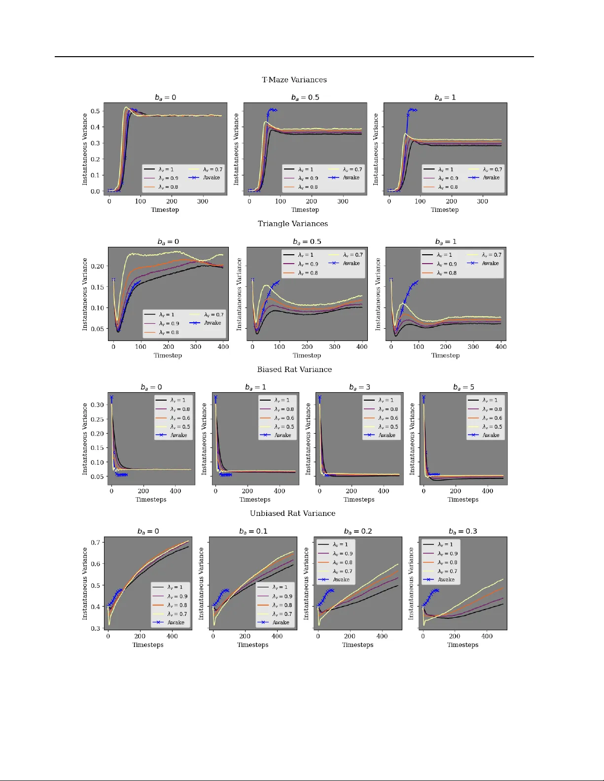
Leakage and Second-Order Dynamics Impr ov e Hippocampal RNN Replay Josue Casco-Rodriguez 1 Nanda H. Krishna 2 Richard G. Baraniuk 1 Abstract Biological neural networks (like the hippocam- pus) can internally generate “replay” resembling stimulus-driv en acti vity . Recent computational models of replay use noisy recurrent neural net- works (RNNs) trained to path-integrate. Replay in these networks has been described as Lange vin sampling, but ne w modiﬁers of noisy RNN replay hav e surpassed this description. W e re-examine noisy RNN replay as sampling to understand or improv e it in three w ays: (1) Under simple as- sumptions, we prov e that the gradients replay ac- tivity should follo w are time-v arying and dif ﬁcult to estimate, b ut readily motiv ate the use of hidden state leakage in RNNs for replay . (2) W e conﬁrm that hidden state adaptation (negati v e feedback) encourages exploration in replay , but show that it incurs non-Markov sampling that also slo ws replay . (3) W e propose the ﬁrst model of tempo- rally compressed replay in noisy path-integrating RNNs through hidden state momentum, connect it to underdamped Lange vin sampling, and sho w that, together with adaptation, it counters slo w- ness while maintaining exploration. W e v erify our ﬁndings via path-integration of 2D triangular and T -maze paths and of high-dimensional paths of synthetic rat place cell activity . 1. Introduction During quiescent periods such as sleep or wak eful resting, some neural circuits internally generate activity resembling that of active periods ( T ingley & Peyrache , 2020 ). Such “replay” phenomena hav e been observed in the prefontal ( Eu- ston et al. , 2007 ; Peyrache et al. , 2009 ), sensory ( K enet et al. , 2003 ; Xu et al. , 2012 ), motor ( Hoffman & McNaughton , 2002 ), and entorhinal cortices ( Gardner et al. , 2022 ); the anterior thalamus ( Pe yrache et al. , 2015 ); and the hippocam- 1 Department of Electrical and Computer Engineering, Rice Univ ersity , USA 2 Mila - Quebec AI Institute & Universit ´ e de Montr ´ eal, Canada. Correspondence to: Josue Casco-Rodriguez < jc135@rice.edu > . Pr eprint. F ebruary 23, 2026. 0 1 2 0 2 4 T ime s ( t ) 0 1 2 T ime r ( t ) 0 1 2 T ime r ( t ) underdamped 0 1 2 T ime r ( t ) w/ adaptation Mean and Std of s ( t ) (awak e paths) and r ( t ) (replay paths) F igur e 1. Underdamped dynamics accelerate ofﬂine replay , adaptation slows it. Here we simulate a noisy RNN r ( t ) that opti- mally path-integrates an Ornstein-Uhlenbeck process s ( t ) from its velocity s ′ ( t ) . W e assume r ( t ) minimizes the loss in Equation ( 8 ) and thus ev olv es according to its scor e function ∇ r ( t ) log p ( r ( t )) (Equations 11 and 15 ), performing a v ariant of Langevin sampling when no input is giv en. Abov e, we compare three modiﬁers of RNN activity: the default (no modiﬁcation, a.k.a. overdamped ), our proposed under damped (momentum), and adaptation (nega- tiv e feedback) dynamics. Each modiﬁer affects the replay distribu- tion p ( r ( t )) in different w ays: underdamped sampling accelerates p ( r ( t )) tow ards p ( s ( t )) , decreasing the distance between them, while adaptation slows con v ergence of p ( r ( t )) tow ards p ( s ( t )) , increasing this distance. pus ( Buzs ´ aki , 1986 ; Skaggs & McNaughton , 1996 ; N ´ adasdy et al. , 1999 ; Lee & Wilson , 2002 ; Foster , 2017 ). Of these circuits, the hippocampus is particularly interesting because its robustness in tasks like navigation ( O’Keefe & Nadel , 1978 ; Burgess et al. , 1994 ; McNaughton et al. , 1996 ) and planning ( Pfeiffer & F oster , 2013 ; Miller et al. , 2017 ) during activ e states seems crucially tied to its spontaneous activ- ity during quiescent states ( Buzs ´ aki , 1989 ; 2015 ; T ononi & Cirelli , 2014 ; ´ Olafsd ´ ottir et al. , 2015 ; 2018 ). While some works ha v e produced replay using supervised generativ e models ( Deperrois et al. , 2022 ), most existing models of hippocampal activity treat replay as an emer- gent byproduct of careful network design. Relev ant net- work parameters include connectivity structures ( Shen & McNaughton , 1996 ; Milstein et al. , 2023 ), local plastic- ity mechanisms ( Hopﬁeld , 2010 ; Litwin-Kumar & Doiron , 2014 ; Theodoni et al. , 2018 ; Haga & Fukai , 2018 ; Asabuki & Fukai , 2025 ), ﬁring rate adaptation ( Chu et al. , 2024 ; Azizi et al. , 2013 ; Itskov et al. , 2011 ; Dong et al. , 2021 ; Li et al. , 2024 ), and input modulation ( Kang & DeW eese , 2019 ). While these models reproduce aspects of replay , they are typically moti v ated by empirical ﬁndings and lack rigorous theoretical justiﬁcation. 1 Leakage and Second-Order Dynamics Impro ve Hippocampal RNN Replay A more principled model of hippocampal function with emergent replay is sequential predicti ve learning ( Krishna et al. , 2024 ; Le v enstein et al. , 2024 ), wherein neural circuits predict dynamic en vironment or task v ariables from imper - fect observations thereof, e.g., path-integrating velocity mea- surements to track a position. This normative description of the hippocampus as a sequence predictor ( Levy , 1989 ; Stachenfeld et al. , 2017 ) matches hippocampal encodings of upcoming stimuli ( Dav achi & DuBrow , 2015 ) and predic- tion errors ( Aitken & Kok , 2022 ; Miller et al. , 2023 ), and neural acti vity sweeps that represent possible future trajec- tories ( Kay et al. , 2020 ; Johnson & Redish , 2007 ). Unlike traditional, hand-crafted models of hippocampal circuits (i.e., continuous attractor networks ( Samsonovich & Mc- Naughton , 1997 ; Battaglia & Tre v es , 1998 )), sequential pre- dictiv e learning models are trained from data. Nonetheless, they account for the emergence of place cells ( Recanatesi et al. , 2021 ; Lev enstein et al. , 2024 ; Chen et al. , 2024 ), grid cells ( Cuev a & W ei , 2018 ; Sorscher et al. , 2019 ), and head direction cells ( Cuev a et al. , 2020 ; Uria et al. , 2022 ); can incorporate phenomena like theta oscillations ( Le v enstein et al. , 2024 ); and exhibit quiescent replay acti vity ( Krishna et al. , 2024 ; Lev enstein et al. , 2024 ; Chen et al. , 2024 ). Krishna et al. ( 2024 ) provided the ﬁrst theoretical foundation for replay in sequential predictiv e learning networks, sho w- ing analytically that they generate diffusi ve replay ( Stella et al. , 2019 ) during quiescent activity (i.e., noise-dri v en ac- ti vity in the absence of inputs) by Langevin sampling ( Besag , 1994 ) from the waking acti vity distribution using its score function. Subsequent empirical work ( Le v enstein et al. , 2024 ) introduced ne w mechanisms to induce exploration in replay through negati v e feedback, i.e., neural adaptation. Exploration is the notion that replay e xpresses a v ariety of behavioral sequences ( Davidson et al. , 2009 ; Pfeif fer , 2020 ), and is associated with long trajectories in neural space, visi- tation of multiple attractor basins, and transitions that were not present in awak e activity . Adaptation can destabilize attractors and induce sudden transitions in replay activity ( Itskov et al. , 2011 ; Dong et al. , 2021 ; Li et al. , 2024 ; Le v- enstein et al. , 2024 ), thereby facilitating exploration, and is thought to play a key role in the dynamics of replay in vivo ( Levenstein et al. , 2019 ). Howev er , existing theory on sequential predicti ve learning cannot account for these mechanisms. Furthermore, sequential predictiv e learning models do not currently account for the tempor al compr es- sion of replay sequences relati v e to awak e sequences of activity ( N ´ adasdy et al. , 1999 ; Buzs ´ aki , 2015 ; Michelmann et al. , 2019 ; Farooq & Dragoi , 2019 ). This phenomenon, which could be caused by short-term facilitation ( Leibold et al. , 2008 ; Jaramillo & Kempter , 2017 ), is not currently captured in replay from any trained RNN model to our knowledge. Overall, while sequential predicti ve learning is a promising model of hippocampal function and replay , its recent em- pirical adv ances ha ve outpaced its theoretical foundations. Moreov er , it is unclear ho w to incorporate phenomena lik e temporal compression in these models, or how inductiv e biases in RNN design affect replay . W e remedy these short- comings by characterizing how RNN design and Lange vin sampling statistics af fect each other . Some results describe how RNN design affects the speed and variance of replay activity , while others start from the Lange vin sampling for - mulation of replay and either explain e xisting architectural choices as useful inducti v e biases, or propose new mecha- nisms to again modulate sampling. In summary , we answer three questions: 1. Optimal path-integration in the presence of noise re- quires RNNs to learn the score function of the noisy activity distrib ution. What is this function, might it in- form RNN design? The score function is time-variant and difﬁcult to estimate , even for simple distributions, but our e xpr ession of it motivates the addition of leak- age (linear dynamics) in RNNs. 2. Adaptation (neg ati ve feedback) empirically induces exploration in replay . How does it affect Langevin sampling? Adaptation induces non-Markov second- or der Lange vin sampling that destabilizes attractors, which can both help (diversify) and hurt (slow) r eplay . 3. T raditional generativ e models beneﬁt from a wide array of sampling techniques. Could ne w sampling meth- ods improve replay in noisy RNNs? Under damped Langevin sampling via momentum quick ens neural r e- play , like temporal compr ession induced by short-term facilitation in vi vo , and mitigates slowing fr om adap- tation while maintaining explor ation. 2. Background In this section, we pro vide background and summarize re- sults from prior work ( Krishna et al. , 2024 ) that has de- scribed replay in path-integrating neural circuits as the sam- pling during quiescence (i.e., the absence of an y inputs) of neural acti vity states from the distrib ution of waking, task- like acti vity . In short, the dynamics of recurrent networks that learn to optimally path-integrate noisy inputs cause the network’ s states ev en in the absence of inputs to resemble those attained during actual task performance. W e also pro- vide details on mechanisms used in the literature to improv e or bias replay , which we e xplore the ef fects of in more detail in this work. For an overvie w of this section, see Section B . 2.1. Langevin Dynamics Langevin sampling from an unkno wn distrib ution p ( x ) en- tails stochastic gradient ascent of an iterate x ( t ) along the 2 Leakage and Second-Order Dynamics Impro ve Hippocampal RNN Replay log-likelihood of p ( x ) via its score function ∇ log p ( x ) or an estimate thereof: ˙ x ( t ) = x ( t ) + ∇ log p ( x ) + √ 2 η ( t ) , (1) where η ( t ) is Gaussian white noise. While Equation 1 de- scribes over damped dynamics, there also exist under damped Langevin dynamics 1 (Equations 2 or 3 , see Chapter 6 of Pa vliotis ( 2014 )) that con verge f aster to the tar get distrib u- tion p ( x ) and better utilize noisy gradients ( Cheng et al. , 2018 ): ¨ x ( t ) = ∇ log p ( x ) − γ ˙ x ( t ) + p 2 γ η ( t ) , or (2) ˙ x ( t ) = v ( t ) , ˙ v ( t ) = ∇ log p ( x ) − γ v ( t ) + p 2 γ η ( t ) (3) In this work, we consider noisy RNNs that have implic- itly learned to perform Lange vin sampling of their own, ﬁxed distributions of activity during task performance, when driv en by just intrinsic noise and in the absence of inputs. That is, the acti vity of the RNNs at each unrolled timestep in the absence of inputs represents a plausible and likely vector of netw ork acti vity during actual task performance in the presence of inputs. In particular , we vie w such networks in the context of replay , where neural circuits recapitulate task-like acti vity e ven during sleep. 2.2. Ofﬂine Replay in RNNs This work focuses on RNNs that implicitly learn to act as generative models ov er a ﬁxed distribution of input se- quences. Krishna et al. ( 2024 ) hav e shown how noisy RNNs trained to path-inte grate their inputs implicitly learn statistics that produce Langevin sampling of their o wn task- rele vant acti vity distrib ution when no input is giv en, demon- strating statistically faithful replay sequences during quies- cence. That is, the RNNs’ activity in the absence of inputs “replays” states from the same distribution as RNN acti vity with inputs during actual task performance. This leads to the generation or “replay” of output sequences resembling those that the network sees during training or task performance with inputs. Path-integration is particularly rele v ant to neu- roscience: animals can leverage motion cues, observ ations, or prior experiences to accurately estimate positions ( Seelig & Jayaraman , 2015 ; Chrastil , 2025 ), and neural circuits like the entorhinal cortex ( Sorscher et al. , 2019 ) hav e been iden- tiﬁed to perform such computations. Here we summarize the ﬁnding that noisy RNNs trained to path-integrate input time-series learn the scor e function of the input distribution ( Krishna et al. , 2024 ). Deﬁnition 2.1. A noisy recurr ent neur al network (RNN) has hidden states r ( t ) that ev olve at each timestep t via some (nonlinear) function of its pre vious hidden states, an input 1 Discretized underdamped Langevin dynamics are a form of Hamiltonian MCMC ( Cheng et al. , 2018 ). signal u ( t ) , and noise: r ( t + ∆ t ) = f ( r ( t ) , u ( t ) , σ r η ( t )) (4) Deﬁnition 2.2. A path-inte gration objecti v e L ( t ) penalizes the difference between a state v ariable s ( t ) and a learnable linear projection of the RNN hidden state r ( t ) : L ( t ) = E η ∥ s ( t ) − D r ( t ) ∥ 2 (5) Assumption 2.3. Krishna et al. ( 2024 ) approximate the hidden state dynamics of a noisy RNN as the sum of two functions 2 and white noise σ r η ( t ) ∼ N (0 , σ 2 r ∆ t ) . ∆ r ( t ) = r ( t + ∆ t ) − r ( t ) ≈ ∆ r 1 ( t ) + ∆ r 2 ( t ) + σ r η ( t ) (6) Assumption 2.4. The optimal r ( t ) minimizes L ( t ) such that p ( r ∗ ( t )) is normal around D † s ( t ) : p ( r ∗ ( t ) | s ( t )) ∼ N ( D † s ( t ) , I σ 2 r ∆ t ) (7) Lemma 2.5. W ith Assumptions 2.3 and 2.4 , L ( t + ∆ t ) is upper bounded by b L ( t + ∆ t ) : b L ( t + ∆ t ) = ∥ s ′ ( t ) − D ∆ r 2 ( t ) ∥ + E η ∥ D σ r η ( t ) ∥ 2 + ∥ D ∥ F E η ∥ ∆ r 1 ( t ) + σ r η ( t − ∆ t ) ∥ 2 (8) Assumption 2.6. The optimal r ( t ) greedily minimizes b L at t only , without concern for long-range dependencies: { r ∗ ( t ) } T t =0 = arg min { r ( t ) } T t =0 Z T t =0 L ( t + ∆ t )∆ t ≈  arg min r ( t ) b L ( t + ∆ t )  T t =0 (9) Theorem 2.7. Given Assumption 2.6 , the optimal update ∆ r ∗ ( t ) = arg min ∆ r 2 ( t ) b L ( t + ∆ t ) + arg min ∆ r 1 ( t ) b L ( t + ∆ t ) + σ r η ( t ) follows s ′ ( t ) and the scor e function of p ( r ( t )) : ∆ r ∗ ( t ) = D † s ′ ( t )∆ t + σ 2 r ∆ t ∇ r ( t ) log p ( r ( t )) + σ r η ( t ) (10) During training, noisy RNNs are (unless otherwise stated, see Section 2.3 ) provided u ( t ) = s ′ ( t ) (or a nonlinear observation thereof) to perform path-integration and focus on denoising. Theorem 2.8. In the absence of input (quiescence), a noisy RNN alr eady tr ained to path-inte grate s ( t ) fr om s ′ ( t ) will perform gradient ascent along the scor e function of r ( t ) . If p ( r ( t )) and p ( s ( t )) ar e stationary , then this ascent is Langevin sampling (Equation 1 ). If the variance of σ r η ( t ) is scaled by a factor of 2, then p ( r ( t )) is guaranteed to con ver ge to the steady-state distribution p ( r ) = p ( D † s ) . If ∆ r ( t ) = σ 2 r ∆ t ∇ r ( t ) log p ( r ( t )) + √ 2 σ r η ( t ) , then lim t →∞ p ( r ( t )) = p ( D † s ) (11) 2 Each function ∆ r 1 ( t ) , ∆ r 2 ( t ) can depend on variables be- yond t , but the y are omitted for concision. 3 Leakage and Second-Order Dynamics Impro ve Hippocampal RNN Replay 2.3. Existing Methods of Biasing Replay in RNNs Neural adaptation. Biological neurons can mitigate pro- longed or lo w-frequency acti vity via negati v e feedback, or adaptation ( Benda , 2021 ; Gutkin & Zeldenrust , 2014 ). This feedback has proven important for describing in vivo hip- pocampal activity and replay ( Itskov et al. , 2011 ; Le v enstein et al. , 2019 ), and in computational models of replay has been shown to encourage long replay trajectories (exploration) by preventing neural acti vations from getting stuck in at- tractor basins ( Dong et al. , 2021 ; Li et al. , 2024 ; Lev enstein et al. , 2024 ). Like Lev enstein et al. ( 2024 ), we deﬁne adap- tation as negati v e feedback c ( t ) added to RNN activity r ( t ) (Equation 4 ) after training 3 : r ( t + ∆ t ) = f ( r ( t ) , u ( t ) , σ r η ( t )) − c ( t ) , ∆ c ( t ) = 1 τ a ( − c ( t ) + b a r ( t )) (12) Masked training. Denoisers and autoencoders beneﬁt from masked tr aining , wherein some re gions of input data are set to zero before model processing ( Zhang et al. , 2023 ). Lev enstein et al. ( 2024 ) introduce masked training for path- integration by periodically masking the input u ( t ) (the ob- servation of s ′ ( t ) ): only at every k -th timestep does the RNN observe a nonzero input (Equation 13 ). u ( t ) = ( s ′ ( t ) , t mod k = 0 0 , otherwise (13) Lev enstein et al. ( 2024 ) found that masked training makes replay sequences more coherent and makes manifolds of neural activity more similar to the spatial layout of the en vi- ronment. W e found that masked training improves replay stability , so we use it (with k ≥ 3 ) in training all RNNs. 3. Estimating the Score Function of Noisy RNN Activity Noisy RNNs trained to path-integrate implicitly learn the score function of their acti vity . Previous works have not examined the score function; in fact, they assume the distri- bution of RNN acti vity p ( r ( t )) is stationary (Theorem 2.8 ), and thus the score function ∇ r ( t ) log p ( r ( t )) depends only on r ( t ) ( Krishna et al. , 2024 ). Howe v er , we refute this assumption, and in doing so reveal the role of leakage in path-integration: ev en if the RNN path-inte grates a simple Gaussian process, the score function requires information beyond r ( t ) , which it emplo ys through linear leakage (de- cay) of r ( t ) . This linearity suggests that leakage is useful for path-integration, which we conﬁrm e xperimentally . 3 Subtraction of the mo ving av erage c ( t ) also arises naturally from greedy minimization of L ( t ) + 1 2 ∥ c ( t ) ∥ 2 2 . 3.1. Challenges in Simple Distributions First, we examine ho w the score function of optimal path- integrating RNN acti vity r ( t ) has nonstationarities that are challenging to perfectly estimate, ev en for simple Gaussian processes. Assumption 3.1. The observ ed states s ( t ) form some Gaus- sian process: p ( s ( t )) ∼ N  µ s ( t ) , Σ s ( t )  . Theorem 3.2. W ith Assumption 3.1 , the score function of trained activity r ( t ) has a closed form whic h, while linear in r ( t ) , is nonlinear with r espect to the par ameters of p ( s ( t )) (see Section C.2 ): σ 2 r ∆ t ∇ r ( t ) log p ( r ( t )) = − Λ ( t )  r ( t ) − D † µ s ( t )  (14) W ith Λ ( t ) = σ 2 r ∆ t  I σ 2 r ∆ t + D † Σ s ( t ) ( D † ) T  − 1 as the leakage matrix of r ( t ) , we can already gain some insight from Equation 14 . Remark 3.3 . If p ( s ( t )) is Gaussian, then the score of p ( r ( t )) is simply a linear function of r ( t ) , but its parameters are non- linear functions of time, and only as stationary as p ( s ( t )) . Remark 3.4 . The eigen v alues of the leakage matrix Λ ( t ) are always between 0 and 1 (see Appendix C.2 ). Moreov er , the eigen v alues of Λ ( t ) and D † Σ s ( t ) ( D † ) T in v ersely correlate: strong decay of r ( t ) implies weak noise Σ r ( t ) , and weak decay of r ( t ) implies strong noise Σ r ( t ) . T o further illustrate ho w estimating the score function of r ( t ) (Equation 14 ) can be challenging, we now examine a scalar RNN r ou ( t ) trained to path-integrate Ornstein-Uhlenbeck processes. Assumption 3.5. The observed states follo w a scalar Ornstein-Uhlenbeck process parameterized by θ , µ, σ s : s ′ ou ( t ) = θ ( µ − s ou ( t )) + σ s η ( t ) , where p ( s (0)) ∼ N (0 , σ 2 0 ) . In other words, p ( s ou ( t )) parameterizes a di- rected random walk from s ou (0) to µ . Remark 3.6 . The score function of the optimal r ou ( t ) under Assumption 3.5 follo ws from Equation ( 26 ) (see Section D ): σ 2 r ∆ t ∇ r ou ( t ) log p ( r ou ( t )) = − σ 2 r ∆ t  r ou ( t ) − µ  1 − e − θt  σ 2 r ∆ t + σ 2 s 2 θ (1 − e − 2 θt ) + σ 2 0 e − θt (15) The score function, and thus the optimal quiescent activity , is evidently complex and nonstationary: lim t → 0 σ 2 r ∆ t ∇ r ou ( t ) log p ( r ou ( t )) = − σ 2 r ∆ t σ 2 r ∆ t + σ 2 0 r ou ( t ) , while lim t →∞ σ 2 r ∆ t ∇ r ou ( t ) log p ( r ou ( t )) = − σ 2 r ∆ t σ 2 r ∆ t + σ 2 s / 2 θ ( r ou ( t ) − µ ) . While one could force stationarity by implicitly assuming the process starts at s ou (0) = µ , or assuming the steady-state dynamics ( t → ∞ ) are the most important, we argue that any 4 Leakage and Second-Order Dynamics Impro ve Hippocampal RNN Replay such approach would miss a fundamentally relev ant aspect of the Ornstein-Uhlenbeck process for navigation: intention . Unlike the Wiener process (Section D ), the Ornstein-Uhlenbeck process can describe a random walk that intentionally navigates from s u (0) to µ , rather than one that simply wanders around µ . Thus, for navigation, the non-stationary , or “early”, dynamics of the Ornstein- Uhlenbeck process are the most salient. Given the rele v ance of non-stationary dynamics for navigation, our analyses focus on the entire course of replay dynamics (rather than steady-state distributions), e xamining properties like speed and path div ersity (e xploration). 3.2. The Advantage of Leakage − 2 0 T raining Iters. Log MSE loss T -Maze Leak No leak − 2 0 T raining Iters. T riangle 1 2 3 1 2 3 k = k = F igur e 2. Leakage helps path-integration. Here we train RNNs on two tasks, ablating the leakage term. Leakage helps training, especially when losses increase with the masking dif ﬁculty k (note that k = 1 is equiv alent to unmasked training, see Equation 13 ). Means are solid, standard deviations are f aint. Theorem 3.2 and Remark 3.3 suggest that linear leakage may be a useful inductive bias for RNNs learning to path- integrate: the score function for a Gaussian process is linear with respect to r ( t ) , although the parameters of said linearity are nonlinear functions of time. W e e xamine the utility of leakage by comparing two RNNs trained to path-inte grate: r ( t + ∆ t ) = κ r ( t ) + f 1 ( r ( t ) , u ( t ) , σ r η ( t )) (RNN with leakage 0 < κ < 1 ) and r ( t + ∆ t ) = f 2 ( r ( t ) , u ( t ) , σ r η ( t )) (RNN without leakage), where f 1 , f 2 are shallow ReLU layers trained separately (see Section A.4 ). The second is more reminiscent of traditional RNNs in machine learning (e.g., ReLU or gated RNNs), which do not typically employ leakage. In Figure 2 , we show that leakage is useful for path-integration, especially with masked training ( k > 1 ). Our results suggest that leakage is a useful component of path-integrating RNNs, although other architectures may be able to successfully learn without it (e.g., the layer-norm RNN of Lev enstein et al. ( 2024 )). 4. Second-Order Langevin Sampling f or Neural Replay In the pre vious section, we examined the score function of trained path-integrating RNN activity . Now , we are as- suming that trained RNNs have well-estimated the score function, and follo w it during quiescent (internally-dri v en) activity to generate replay via Lange vin dynamics. Here we ask how modulating the dynamics of such RNNs affects the distribution of replay—in other words, how changing the RNN dynamics biases the distrib ution of replay . W e see that adaptation (negati ve feedback) incurs a non-ideal form of second-order Langevin sampling, so we propose a comple- mentary alternativ e that e xplicitly performs underdamped second-order sampling. 4.1. Adaptation as Underdamped Langevin Dynamics First we examine adaptation (negati v e feedback), as deﬁned in Section 2.3 . Proposition 4.1. Adding adaptation (Equation ( 12 ) ) to a trained path-inte gr ating RNN during quiescence (Equa- tion ( 11 ) ) incurs Langevin sampling with ne gative feedbac k: ∆ r ( t ) = σ 2 r ∆ t ∇ r ( t ) log p ( r ( t )) + √ 2 σ r η ( t ) − c ( t ) , ∆ c ( t ) = 1 τ a ( − c ( t ) + b a r ( t )) (16) For the clearest illustration of the ef fects of adaptation, let us examine a stationary p ( r ( t )) —a simpliﬁcation which we argued in Section 3.1 is not realistic, but is nonetheless intuitiv e. Assumption 4.2. The observed states are normal (Assump- tion 3.1 ) and stationary: p ( s ( t )) ∼ N ( µ , Σ ) . Theorem 4.3. Adding adaptation to an RNN tr ained to path-inte gr ate states drawn fr om a stationary Gaussian dis- tribution (Assumption 4.2 and Equation ( 16 ) ) pr oduces the following second-or der stoc hastic dynamics during quies- cence (see Section E ): r ′′ ( t ) =  b a τ a I + σ 2 r ∆ t d 2 d r ( t ) 2 log p ( r ( t ))  r ′ ( t ) − b a τ a σ 2 r ∆ t ∇ r ( t ) log p ( r ( t )) + 1 τ a r ( t ) − σ b a τ a η ( t ) + σ η ′ ( t ) (17) Comparing Equation 17 with Equation 2 , the two indeed resemble each other: adaptation seems to induce a form of underdamped Langevin dynamics. This may help explain the observed utility of adaptation for generating replay ( It- skov et al. , 2011 ; Le v enstein et al. , 2019 ; 2024 ). Moreover , since we established in Section 3 that the score function of e ven a basic stochastic process is difﬁcult to estimate, the effecti veness of underdamped Langevin sampling for working with noisy gradients ( Cheng et al. , 2018 ) may be useful when ∇ r ( t ) log p ( r ( t )) is poorly estimated. Howe ver , interpreting Equation ( 17 ) as underdamped Langevin sampling re v eals some shortcomings thereof as a sampling method. 5 Leakage and Second-Order Dynamics Impro ve Hippocampal RNN Replay Remark 4.4 . The coef ﬁcient of r ′ ( t ) is usually constant, and should be positi ve to ensure con vergence ( P a vliotis ( 2014 ), pg. 183), b ut b a τ a I + ∇ r ( t ) log p ( r ( t )) is not constant and could be negati v e. Remark 4.5 . Underdamped Langevin sampling from r ( t ) should not hav e a negati v e sign in front of ∇ r ( t ) log p ( r ( t )) if the intention is to maximize p ( r ( t )) . 4.2. Replay via Explicit Underdamped Langevin Dynamics While adaptation is a biologically plausible way to perform a variant of underdamped Lange vin dynamics in RNNs, we propose an alternativ e method, from Equation 3 , to more clearly and directly perform underdamped Langevin sam- pling. It is conceptually similar to RNNs with momentum ( Nguyen et al. , 2020 ): a v elocity term v ( t ) accumulates previous r ( t ) v alues when friction λ v ∈ [0 , 1] is belo w 1 4 . Deﬁnition 4.6. W e implement explicitly under damped dy- namics via momentum governed by friction λ v . When λ v = 1 , dynamics rev ert to o verdamped (Equation ( 4 )): v ( t +∆ t ) = (1 − λ v ) v ( t )+ f ( r ( t ) , u ( t ) , σ r η ( t )) − r ( t ) | {z } ∆ r ( t ) if λ v =1 , ∆ r ( t ) = v ( t + ∆ t ) (18) Biological plausibility . Se veral previous works in theo- retical neuroscience ha ve proposed mechanisms in v olving momentum, including Hamiltonian dynamics, for f ast and improv ed sampling ( Hennequin et al. , 2014 ; Masset et al. , 2022 ; Furlong et al. , 2024 ; Dong & W u , 2023 ; Aitchison & Lengyel , 2016 ; Dong et al. , 2022 ). Some have implemented these dynamics in E/I or spiking netw orks. Thus, it is con- ceiv able that the brain could use momentum to quickly and efﬁciently sample ( Hennequin et al. , 2014 ). Additionally , sampling schemes with momentum improve modeling of human random sequence generation ( Castillo et al. , 2024 ), and momentum has been found in hippocampal replay tra- jectories ( Krause & Drugo witsch , 2022 ). W e propose mo- mentum as a circuit mechanism for temporal compression in replay , but we cannot directly compare it to the physio- logical mechanisms behind temporal compression in vivo because they are not yet fully understood. Nonetheless, we identify two mechanisms for which momentum may be a reasonable initial approximation: (1) Short-term facilita- tion can induce phase precession and temporal compression in spiking networks ( Leibold et al. , 2008 ). Extensions to rate networks are scant, so momentum may be a reasonable initial approximation. (2) Short-term post-synaptic plastic- ity via NMD A receptors induces momentum-like ef fects in continuous attractor networks ( Zhao et al. , 2023 ). 4 For a comparison of λ v and the γ term from Equations 3 and 2 , see Section A.5 . 5. Numerical Results Now we examine how adaptation and underdampening (Equations 12 and 18 ) bias replay distributions in trained path-integrating RNNs. W e ﬁrst see the y counter each other: adaptation slows replay , while underdampening quickens it. Then we conﬁrm that adaptation induces exploration, and show that underdampening does not pre v ent exploration, but rather complements it by increasing path lengths. W e note here that replay trajectories are obtained by ﬁrst ran- domly initializing the hidden state of the RNN, following which we collect acti v ations for se veral unrolled timesteps in the absence of inputs but in the presence of noise. Fur- ther details are provided in Appendix A.1 . Here we use ReLU and leaky ReLU trained RNNs, as justiﬁed in Sec- tion A.2 , but in Section G we conﬁrm that adaptation slows and underdampening compresses replay in tanh RNNs. Experiments. W e hav e ﬁv e tasks on which we train RNNs and then examine how introducing sampling mechanisms post-training (adaptation strength b a and friction λ v ) affects replay (quiescent activity) statistics. W e explain our imple- mentation and many measured replay statistics in Section A . 1. 1D Ornstein-Uhlenbeck (OU) process (Figure 1 ): the optimal (with respect to Equation ( 8 )) path-integrating RNN has a closed form (Equation ( 15 )), which we use in lieu of a trained RNN. 2. 2D T -maze and triangle (Figure 3 ): we simulate each direction (two in T -maze, six in triangle) as a 2D OU process, and train a ReLU RNN to integrate 2D paths from ev ery direction. 3. Rat trajectories (Section F , Figure 8 ): like Krishna et al. ( 2024 ), we simulate 512 place cells that encode 2D directed (biased) or undirected (unbiased) random walks from RatInABox ( George et al. , 2024 ), train a ReLU RNN to path-integrate place cell activity , and decode activity in 2D. W e use in silico rat activity to mimic biological data because replay events in vivo are sparse and dif ﬁcult to e xtract from background noisy activity , therefore outside the scope of this work. Underdampening and adaptation seem to counter each other . W e initially observe that the two modiﬁers coun- teract each other: in Figures 1 and 3 , adaptation repels trajectories away from attractors (such as endpoints), while underdampening accelerates trajectories to wards them. This makes sense gi v en Remark 4.5 and the nature of under- damped sampling. Then we measure how the two modiﬁers affect the similarity between replay (internally-dri ven) and awak e (observed) trajectories. Figure 4 sho ws they both generally decrease the similarity to a wak e trajectories, b ut 6 Leakage and Second-Order Dynamics Impro ve Hippocampal RNN Replay T -maze T riangle • = endpoint (a) Overdamped Adaptation ( b a = 1 ) Overdamped Adaptation ( b a = 1 ) Underdamped ( λ v = 0 . 7 ) Underdamped + Adaptation Underdamped ( λ v = 0 . 7 ) Underdamped + Adaptation 1 0 1 0 − 1 0 1 − 1 0 1 1 0 1 0 0 1 0 1 (b) (c) F igur e 3. Underdampening and adaptation counter each other . Here we show replay from RNNs trained to path-integrate in T -maze or triangular en vironments. (a) A wake paths in each task form a mixture of Ornstein-Uhlenbeck processes, one for each direction of trav el. A wak e paths reach their endpoints and stay there. In (b) and (c) are mean replay paths (darkening o ver time) from T -maze and triangle tasks, simulated for the same time as awake paths. Standard deviations are faint, ideal path means are dashed. Like in Figure 1 , adaptation slows con vergence to wards endpoints, underdampening quick ens it. Also, the two mechanisms induce deviations that neg ate each other . 0 . 8 1 0 10 Friction λ v W asserstein distance ( ↓ ) T -maze 0.0 0.5 1.0 0 . 8 1 0 2 4 Friction λ v T riangle 0 . 6 0 . 8 1 0 . 08 0 . 1 0 . 12 Friction λ v Biased rat 0 1 3 5 1 0 . 9 0 . 8 0 . 7 0 . 11 0 . 12 0 . 13 Friction λ v Unbiased rat 0.0 0.1 0.2 0.3 Adaptation strength b a : F igur e 4. Underdampening impro ves replay ﬁdelity in the presence of adaptation. W e compute the W asserstein distance (dissimilarity) between awak e and replay path distrib utions ( p ( { s ( t ) } T t =0 ) and p ( { r ( t ) } T t =0 ) ), varying friction and adaptation strength (see Section A for details). While the two mechanisms both generally increase this distance, underdampening ( λ v < 1 ) decreases it if adaptation is nonzero. Like in Figure 3 , underdampening counters adaptation-induced deviations. they do counter each other insofar as underdampening, in the presence of adaptation, increases similarity to awake trajectories. Thus far , underdampening counters adaptation qualitativ ely and statistically . Adaptation slows replay , underdampening accelerates it. Next, we e xamine a key component of replay: speed. In Fig- ures 4 and 5 , we generally see that adaptation slo ws replay or increases the dissimilarity between replay and awake tra- jectories. The exception is the biased rat trajectories, since they are the only task where all trajectories reach the same common goal. Such path distributions resemble Ornstein- Uhlenbeck processes with steady-state mean µ = 0 : in such cases, adaptation actually accelerates con v ergence to w ards the steady-state. In Figure 5 , we see that underdampening increases replay speed, performing temporal compression relativ e to a wake acti vity . Underdampening complements exploration from adap- tation. W e have established that underdampening coun- ters adaptation, both qualitativ ely and in terms of speed. Howe ver , we do not w ant to merely propose a mechanism 0 0 . 5 1 1 0 . 9 0 . 8 0 . 7 Friction λ v T -maze − 30 0 60 120 0 0 . 5 1 1 0 . 9 0 . 8 0 . 7 Adaptation strength b a T riangle − 30 0 55 110 0 1 3 5 1 0 . 8 0 . 6 0 . 5 Biased rat − 60 0 150 300 Change (%) from awak e reach time: Median replay reach time ( ↓ ) F igur e 5. Underdampening temporally compresses r eplay . W e calculate how long it takes aw ake and replay trajectories to reach their endpoints. Underdampening ( λ v < 1 ) not only shortens this reach time, but makes it smaller than that of awake paths, temporally compressing awake acti vity . See Section F Figure 9 for mean reach times. W e do not include unbiased rat trajectories because they do not ha ve deﬁned endpoints, b ut we do conﬁrm in Section F Figure 10 that underdampening quickens them. 7 Leakage and Second-Order Dynamics Impro ve Hippocampal RNN Replay 0 . 8 1 8 8 . 5 Friction λ v Mean path length ( ↑ ) T -maze 0.0 0.5 1.0 0 . 8 1 8 . 5 9 Friction λ v T riangle 0 . 6 0 . 8 1 3 4 Friction λ v Biased rat 0 1 3 5 0 . 8 1 3 3 . 5 4 Friction λ v Unbiased rat 0.0 0.1 0.2 0.3 Adaptation strength b a : F igur e 6. On average, underdampening increases exploration via path length. In here and Figure 7 we simulate replay paths for more time than awak e paths, varying friction and adaptation strength. Shown abov e, underdampening ( λ v < 1 ) increases the average length of replay paths. It may do so via increased replay speeds (Section F Figure 10 ) or via additional path transitions (Figure 7 ); the latter is how adaptation increases path length. Regions visited ( ↑ ) • = 2 • , • = 3 • = 4 (a) Examples of exploration in replay: 0 . 8 1 2 2 . 1 Friction λ v A verage regions visited ( ↑ ) T -maze 0.0 0.5 1.0 0 . 8 1 2 2 . 5 Friction λ v T riangle Adaptation strength b a : (c) On av erage, λ v < 1 increases e xploration. (i) increase exploration (ii) decrease exploration (iii) not affect exploration r .v . = 2 . 0 r.v. = 4 . 0 r .v . = 3 . 0 r .v . = 3 . 2 r.v. = 3 . 0 r .v . = 3 . 0 1 0 1 0 0 1 0 1 0 1 λ v = 1 λ v = 0.7 (b) Underdampening ( λ v < 1 ) might: r .v . = mean regions visited, • = start, × = end F igur e 7. On average, underdampening incr eases exploration via regions visited. Another relev ant aspect of exploration is transitions not present in awake acti vity . (a) Here we quantify these transitions via re gions visited . Each region is an area where every point is closest to the same endpoint. In our T -maze and triangle tasks, aw ake paths go from starting points to endpoints and stay there, visiting two regions total (starting and ending). Meanwhile, adaptation ( b a = 1 ) can make replay paths visit multiple endpoints (regions visited ¿ 2). (b) When we use adaptation and underdampening ( λ v < 1 ), we see that replay paths might visit (i) more, (ii) fewer , or (iii) the same regions (see Section F Figure 12 for more details). (c) Ho wev er , on av erage, across se veral different trained models, underdampening increases regions visited, thus increasing adaptation. that undoes adaptation. Adaptation can induce exploration, i.e., prev ent replay trajectories from getting stuck in attrac- tors. W e ﬁnd that underdampening does not on average pre- vent adaptation-induced e xploration. In fact, underdampen- ing complements adaptation for exploration: underdamped paths travel farther (Figures 6 and 7 ), hav e more variance (Section F Figure 11 ), and generally exhibit the same, if not more, exploratory behavior as the y did with only adaptation (Figure 7 ). Underdampening maintains exploration while counteracting the slowness from adaptation. 6. Conclusions and Future W ork W e ha ve re-applied Langevin sampling theory to replay in sequential predicti ve learning netw orks, producing theoret- ically and conﬁrming empirically three key insights: (1) estimating the per-timestep score function of RNN acti v- ity is challenging, but does beneﬁt from linear leakage; (2) adaptation (negati v e feedback) is a variant of underdamped Langevin sampling that encourages e xploration (as sho wn in prior works) but also slows replay; (3) our new under- dampening mechanism (momentum) temporally compresses replay while also increasing exploration from adaptation. These ﬁndings improv e our understanding of biological neural networks that produce replay , like the hippocampus. Our proposed underdampening mechanism via momentum could be tied to short-term facilitation (which can be probed experimentally), connected to speciﬁc subregions in the hippocampus (lik e Chen et al. ( 2024 )), or reﬁned through in- sights from existing RNNs with momentum ( Nguyen et al. , 2020 ). Future efforts could conﬁrm our ﬁndings in more complex en vironments ( W ood et al. , 2018 ; Lev enstein et al. , 2024 ). Like preceding works, our network models are rate- based, b ut extending our work to spike-based models of replay and sequential predicti ve learning ( Saponati & V inck , 2023 ; Asabuki & Fukai , 2025 ; Bono et al. , 2023 ) would be interesting (i.e., extending Langevin sampling to Poisson processes). Sev eral av enues remain for connecting Langevin sampling to neural replay . 8 Leakage and Second-Order Dynamics Impro ve Hippocampal RNN Replay Impact Statement This work aims to advance our understanding of the com- putations underlying replay in the brain. It is a theoreti- cal study that aims to adv ance our understanding of neuro- science through the use of artiﬁcial neural network models, as is common in computational neuroscience. There may be man y potential societal consequences of our work in the long-term, none of which we feel must be speciﬁcally highlighted here. Reproducibility Statement For our theoretical contrib utions, i.e., Theorems 3.2 and 4.3, we provide proofs in Appendix C and E (proofs for Theo- rems 2.7 and 2.8 may be found in Section 2 of Krishna et al. ( 2024 )). Details on our numerical experiments, including associated hyperparameters and implementation details are provided in Appendix A . Our code has been submitted as Supplementary Material (see README.md for instructions) and will be made publicly av ailable upon publication. References Aitchison, L. and Lengyel, M. The Hamiltonian brain: Ef ﬁcient probabilistic inference with excitatory-inhibitory neural circuit dynamics. PLoS Computational biology , 12(12), 2016. Aitken, F . and Kok, P . Hippocampal representations switch from errors to predictions during acquisition of predicti ve associations. Natur e Communications , 13(1), 2022. Alemohammad, S., Casco-Rodriguez, J., Luzi, L., Hu- mayun, A. I., Babaei, H., LeJeune, D., Siahkoohi, A., and Baraniuk, R. G. Self-consuming generative mod- els go MAD. In International Conference on Learning Repr esentations (ICLR) , 2024. Ali, A., Ahmad, N., de Groot, E., van Gerven, M. A. J., and Kietzmann, T . C. Predicti v e coding is a consequence of energy ef ﬁcienc y in recurrent neural networks. P atterns , 3(12), 2022. Asabuki, T . and Fukai, T . Predictiv e learning rules generate a cortical-like replay of probabilistic sensory experiences. eLife , 13, 2025. Azizi, A. H., W iskott, L., and Cheng, S. A computational model for preplay in the hippocampus. F r ontiers in com- putational neur oscience , 7:161, 2013. Battaglia, F . P . and T re v es, A. Attractor neural networks storing multiple space representations: a model for hip- pocampal place ﬁelds. Physical Revie w E , 58(6), 1998. Benda, J. Neural adaptation. Curr ent Biology , 31(3), 2021. Besag, J. E. Discussion of “Representations of knowledge in complex systems” by Ulf Grenander and Michael I Miller. Journal of the Royal Statistics Society B , 56(4): 591–592, 1994. Bonneel, N., Rabin, J., Peyr ´ e, G., and Pﬁster , H. Sliced and radon wasserstein barycenters of measures. Journal of Mathematical Imaging and V ision , 51(1), 2015. Bono, J., Zannone, S., Pedrosa, V ., and Clopath, C. Learning predictiv e cognitive maps with spiking neurons during behavior and replays. Elife , 12, 2023. Burgess, N., Recce, M., and O’Keefe, J. A model of hip- pocampal function. Neural networks , 7(6-7), 1994. Buzs ´ aki, G. Hippocampal sharp wav es: their origin and signiﬁcance. Brain r esear ch , 398(2), 1986. Buzs ´ aki, G. T wo-stage model of memory trace formation: a role for “noisy” brain states. Neur oscience , 31(3), 1989. Buzs ´ aki, G. Hippocampal sharp wav e-ripple: A cognitiv e biomarker for episodic memory and planning. Hippocam- pus , 25(10), 2015. Castillo, L., Le ´ on-V illagr ´ a, P ., Chater , N., and Sanborn, A. Explaining the ﬂa ws in human random generation as local sampling with momentum. PLOS Computational Biology , 20(1), 2024. Chen, Y ., Zhang, H., Cameron, M., and Sejno wski, T . Pre- dictiv e sequence learning i n the hippocampal formation. Neur on , 112(15), 2024. Cheng, X., Chatterji, N. S., Bartlett, P . L., and Jordan, M. I. Underdamped Langevin MCMC: A non-asymptotic anal- ysis. In Pr oceedings of the 31st Conference On Learning Theory , volume 75, 2018. Chettih, S. N., Macke vicius, E. L., Hale, S., and Aronov , D. Barcoding of episodic memories in the hippocampus of a food-caching bird. Cell , 187(8), 2024. Chrastil, E. R. Human path integration and the neu- ral underpinnings. In Encyclopedia of the Human Brain (Second Edition) , pp. 157–170. Elsevier , 2025. ISBN 978-0-12-820481-8. doi: https://doi.org/10.1016/ B978- 0- 12- 820480- 1.00016- 4. Chu, T ., Ji, Z., Zuo, J., Mi, Y ., Zhang, W ., Huang, T ., Bush, D., Bur gess, N., and W u, S. Firing rate adaptation affords place cell theta sweeps, phase precession and procession. bioRxiv , 2024. Churchland, M. M. and Shenoy , K. V . Preparatory acti vity and the expansi ve null-space. Natur e Reviews Neur o- science , 25(4), 2024. 9 Leakage and Second-Order Dynamics Impro ve Hippocampal RNN Replay Croitoru, F .-A., Hondru, V ., Ionescu, R. T ., and Shah, M. Diffusion models in vision: A survey . IEEE T ransac- tions on P attern Analysis and Machine Intelligence , 45 (9), 2023. Cuev a, C. J. and W ei, X.-X. Emer gence of grid-lik e repre- sentations by training recurrent neural networks to per- form spatial localization. In International Confer ence on Learning Repr esentations , 2018. Cuev a, C. J., W ang, P . Y ., Chin, M., and W ei, X.-X. Emer- gence of functional and structural properties of the head direction system by optimization of recurrent neural net- works. In International Conference on Learning Repr e- sentations , 2020. Dav achi, L. and DuBrow , S. How the hippocampus pre- serves order: the role of prediction and context. T r ends in cognitive sciences , 19(2), 2015. Davidson, T . J., Kloosterman, F ., and W ilson, M. A. Hip- pocampal replay of extended e xperience. Neur on , 63(4), 2009. Deperrois, N., Petrovici, M. A., Senn, W ., and Jordan, J. Learning cortical representations through perturbed and adversarial dreaming. eLife , 11:e76384, 2022. ISSN 2050-084X. Dong, X. and W u, S. Neural sampling in hierarchical exponential-family energy-based models. Advances in Neural Information Pr ocessing Systems (NeurIPS) , 36, 2023. Dong, X., Chu, T ., Huang, T ., Ji, Z., and W u, S. Noisy adaptation generates L ´ evy ﬂights in attractor neural net- works. Advances in Neural Information Pr ocessing Sys- tems (NeurIPS) , 34, 2021. Dong, X., Ji, Z., Chu, T ., Huang, T ., Zhang, W ., and W u, S. Adaptation accelerating sampling-based bayesian in- ference in attractor neural networks. Advances in Neural Information Pr ocessing Systems (NeurIPS) , 35, 2022. Euston, D. R., T atsuno, M., and McNaughton, B. L. Fast- forward playback of recent memory sequences in pre- frontal cortex during sleep. Science , 318(5853):1147– 1150, 2007. Farooq, U. and Dragoi, G. Emergence of preconﬁgured and plastic time-compressed sequences in early postnatal dev elopment. Science , 363(6423), 2019. Foster , D. J. Replay comes of age. Annual Review of Neur oscience , 40:581–602, 2017. ISSN 1545-4126. Furlong, P . M., Simone, K., Dumont, N. S.-Y ., Bartlett, M., Ste wart, T . C., Orchard, J., and Eliasmith, C. Biologically- plausible Markov Chain Monte Carlo sampling from vec- tor symbolic algebra-encoded distributions. In Interna- tional Confer ence on Artiﬁcial Neur al Networks , 2024. Gardner , R. J., Hermansen, E., Pachitariu, M., Burak, Y ., Baas, N. A., Dunn, B. A., Moser, M.-B., and Moser , E. I. T oroidal topology of population activity in grid cells. Natur e , 602(7895):123–128, 2022. ISSN 1476-4687. George, T . M., Rastogi, M., de Cothi, W ., Clopath, C., Stachenfeld, K., and Barry , C. RatInABox, a toolkit for modelling locomotion and neuronal activity in continuous en vironments. eLife , 13:e85274, 2024. ISSN 2050-084X. Gozalo-Brizuela, R. and Garrido-Merchan, E. C. ChatGPT is not all you need. a state of the art revie w of large generativ e AI models. arXiv preprint , 2023. Gutkin, B. and Zeldenrust, F . Spike frequency adaptation. Scholarpedia , 9(2), 2014. Haga, T . and Fukai, T . Recurrent network model for learning goal-directed sequences through re verse replay . eLife , 7: e34171, 2018. ISSN 2050-084X. Hennequin, G., Aitchison, L., and Lengyel, M. Fast sampling-based inference in balanced neuronal networks. Advances in Neural Information Pr ocessing Systems (NeurIPS) , 27, 2014. Hoffman, K. L. and McNaughton, B. L. Coordinated reacti- vation of distrib uted memory traces in primate neocortex. Science , 297(5589):2070–2073, 2002. Hopﬁeld, J. J. Neurodynamics of mental exploration. Pr o- ceedings of the National Academy of Sciences , 107(4): 1648–1653, 2010. Itskov , V ., Curto, C., Pastalko v a, E., and Buzs ´ aki, G. Cell assembly sequences arising from spike threshold adapta- tion keep track of time in the hippocampus. Journal of Neur oscience , 31(8), 2011. Jaramillo, J. and Kempter , R. Phase precession: a neural code underlying episodic memory? Curr ent Opinion in Neur obiolo gy , 43, 2017. Johnson, A. and Redish, A. D. Neural ensembles in CA3 transiently encode paths forward of the animal at a deci- sion point. J ournal of Neur oscience , 27(45), 2007. Kang, L. and DeW eese, M. R. Replay as wav efronts and theta sequences as bump oscillations in a grid cell attrac- tor network. eLife , 8:e46351, 2019. ISSN 2050-084X. 10 Leakage and Second-Order Dynamics Impro ve Hippocampal RNN Replay Kay , K., Chung, J. E., Sosa, M., Schor , J. S., Karlsson, M. P ., Larkin, M. C., Liu, D. F ., and Frank, L. M. Constant sub-second cycling between representations of possible futures in the hippocampus. Cell , 180(3), 2020. Kenet, T ., Bibitchkov , D., Tsodyks, M., Grinv ald, A., and Arieli, A. Spontaneously emerging cortical representa- tions of visual attributes. Nature , 425(6961):954–956, 2003. ISSN 1476-4687. Krause, E. L. and Drugowitsch, J. A large majority of awak e hippocampal sharp-wav e ripples feature spatial trajectories with momentum. Neur on , 110(4), 2022. Krishna, N. H., Bredenberg, C., Levenstein, D., Richards, B. A., and Lajoie, G. Suf ﬁcient conditions for ofﬂine reacti vation in recurrent neural networks. In International Confer ence on Learning Repr esentations (ICLR) , 2024. Lee, A. K. and W ilson, M. A. Memory of sequential experi- ence in the hippocampus during slow wav e sleep. Neur on , 36(6):1183–1194, 2002. ISSN 0896-6273. Leibold, C., Gundlﬁnger, A., Schmidt, R., Thurley , K., Schmitz, D., and K empter , R. T emporal compression mediated by short-term synaptic plasticity . Pr oceedings of the National Academy of Sciences , 105(11), 2008. Lev enstein, D., Buzs ´ aki, G., and Rinzel, J. NREM sleep in the rodent neocortex and hippocampus reﬂects e xcitable dynamics. Natur e Communications , 10(1), 2019. Lev enstein, D., Efremov , A., Eyono, R. H., Peyrache, A., and Richards, B. Sequential predictive learning is a uni- fying theory for hippocampal representation and replay . bioRxiv , 2024. Levy , W . B. A computational approach to hippocampal function. In Psycholo gy of learning and motivation , vol- ume 23. Elsevier , 1989. Li, X., Thickstun, J., Gulrajani, I., Liang, P . S., and Hashimoto, T . B. Diffusion-LM improves controllable text generation. Advances in Neur al Information Pr ocess- ing Systems (NeurIPS) , 35, 2022. Li, Y ., Chu, T ., and W u, S. Dynamics of adaptiv e continuous attractor neural networks. arXiv pr eprint arXiv:2410.06517 , 2024. Litwin-Kumar , A. and Doiron, B. Formation and mainte- nance of neuronal assemblies through synaptic plasticity . Natur e Communications , 5(1):5319, 2014. ISSN 2041- 1723. Luzi, L., Mayer , P . M., Casco-Rodriguez, J., Siahkoohi, A., and Baraniuk, R. Boomerang: Local sampling on image manifolds using diffusion models. T ransactions on Machine Learning Resear ch (TMLR) , 2024. Masset, P ., Zav atone-V eth, J., Connor , J. P ., Murthy , V ., and Pehlev an, C. Natural gradient enables fast sampling in spiking neural networks. Advances in Neur al Information Pr ocessing Systems (NeurIPS) , 35, 2022. McNamee, D. C., Stachenfeld, K. L., Botvinick, M. M., and Gershman, S. J. Flexible modulation of sequence generation in the entorhinal–hippocampal system. Natur e Neur oscience , 24(6), 2021. McNaughton, B. L., Barnes, C. A., Gerrard, J. L., Gothard, K., Jung, M. W ., Knierim, J. J., Kudrimoti, H., Qin, Y ., Sk- aggs, W ., Suster, M., et al. Deciphering the hippocampal polyglot: the hippocampus as a path inte gration system. Journal of Experimental Biolo gy , 199(1), 1996. Michelmann, S., Staresina, B. P ., Bowman, H., and Hanslmayr , S. Speed of time-compressed forward re- play ﬂexibly changes in human episodic memory . Natur e Human Behaviour , 3(2), 2019. Miller , A. M., Jacob, A. D., Ramsaran, A. I., De Snoo, M. L., Josselyn, S. A., and Frankland, P . W . Emer gence of a predicti ve model in the hippocampus. Neur on , 111 (12), 2023. Miller , K. J., Botvinick, M. M., and Brody , C. D. Dorsal hip- pocampus contributes to model-based planning. Nature neur oscience , 20(9), 2017. Milstein, A. D., Tran, S., Ng, G., and Soltesz, I. Ofﬂine memory replay in recurrent neuronal networks emer ges from constraints on online dynamics. The J ournal of Physiology , 601(15):3241–3264, 2023. Miyasawa, K. An empirical Bayes estimator of the mean of a normal population. Bulletin of the International Statistical Institute , 38(4):181–188, 1961. N ´ adasdy , Z., Hirase, H., Czurk ´ o, A., Csicsvari, J., and Buzs ´ aki, G. Replay and time compression of recurring spike sequences in the hippocampus. Journal of Neur o- science , 19(21):9497–9507, 1999. ISSN 0270-6474. Nguyen, T ., Baraniuk, R., Bertozzi, A., Osher , S., and W ang, B. MomentumRNN: Integrating momentum into recur- rent neural networks. Advances in Neural Information Pr ocessing Systems (NeurIPS) , 33, 2020. O’Keefe, J. and Nadel, L. The hippocampus as a cognitive map . Oxford Uni versity Press, 1978. Panaretos, V . M. and Zemel, Y . Statistical aspects of w asser - stein distances. Annual Revie w of Statistics and its Appli- cation , 6(1), 2019. Pa vliotis, G. A. Stochastic processes and applications. T exts in Applied Mathematics , 60, 2014. 11 Leakage and Second-Order Dynamics Impro ve Hippocampal RNN Replay Peyrache, A., Khamassi, M., Benchenane, K., W iener , S. I., and Battaglia, F . P . Replay of rule-learning related neural patterns in the prefrontal cortex during sleep. Natur e Neur oscience , 12(7):919–926, 2009. ISSN 1546-1726. Peyrache, A., Lacroix, M. M., Petersen, P . C., and Buzs ´ aki, G. Internally or ganized mechanisms of the head direction sense. Natur e Neur oscience , 18(4):569–575, 2015. ISSN 1546-1726. Pfeiffer , B. E. The content of hippocampal “replay”. Hip- pocampus , 30(1), 2020. Pfeiffer , B. E. and Foster , D. J. Hippocampal place-cell se- quences depict future paths to remembered goals. Nature , 497(7447), 2013. Recanatesi, S., Farrell, M., Lajoie, G., Dene v e, S., Rigotti, M., and Shea-Brown, E. Predicti v e learning as a network mechanism for e xtracting lo w-dimensional latent space representations. Natur e Communications , 12(1), 2021. Samsonovich, A. and McNaughton, B. L. Path integration and cognitive mapping in a continuous attractor neural network model. Journal of Neur oscience , 17(15), 1997. Saponati, M. and V inck, M. Sequence anticipation and spike-timing-dependent plasticity emer ge from a predic- tiv e learning rule. Nature Communications , 14(1), 2023. Seelig, J. D. and Jayaraman, V . Neural dynamics for land- mark orientation and angular path integration. Nature , 521(7551), 2015. Shen, B. and McNaughton, B. L. Modeling the spontaneous reactiv ation of experience-speciﬁc hippocampal cell as- sembles during sleep. Hippocampus , 6(6):685–692, 1996. Skaggs, W . E. and McNaughton, B. L. Replay of neuronal ﬁring sequences in rat hippocampus during sleep follow- ing spatial experience. Science , 271(5257), 1996. Song, Y . and Ermon, S. Generativ e modeling by estimating gradients of the data distribution. In Advances in Neural Information Pr ocessing Systems (NeurIPS) , v olume 32, 2019. Sorscher , B., Mel, G., Ganguli, S., and Ocko, S. A uniﬁed theory for the origin of grid cells through the lens of pattern formation. In W allach, H. M., Larochelle, H., Beygelzimer , A., d’Alch ´ e Buc, F ., Fox, E. B., and Garnett, R. (eds.), Advances in Neural Information Pr ocessing Systems , volume 32. Curran Associates, Inc., 2019. Stachenfeld, K. L., Botvinick, M. M., and Gershman, S. J. The hippocampus as a predictiv e map. Natur e neur o- science , 20(11), 2017. Stella, F ., Baracskay , P ., O’Neill, J., and Csicsv ari, J. Hip- pocampal reactiv ation of random trajectories resembling brownian dif fusion. Neur on , 102(2), 2019. T ang, M., Barron, H., and Bogacz, R. Sequential memory with temporal predicti ve coding. In Advances in Neural Information Pr ocessing Systems (NeurIPS) , v olume 36, 2023. T ang, M., Barron, H., and Bogacz, R. Learning grid cells by predicti ve coding. arXiv pr eprint arXiv:2410.01022 , 2024. Theodoni, P ., Rovira, B., W ang, Y ., and Roxin, A. Theta- modulation driv es the emergence of connecti vity patterns underlying replay in a network model of place cells. eLife , 7:e37388, 2018. ISSN 2050-084X. T ingley , D. and Peyrache, A. On the methods for reacti- vation and replay analysis. Philosophical T ransactions of the Royal Society B: Biolo gical Sciences , 375(1799): 20190231, 2020. T ononi, G. and Cirelli, C. Sleep and the price of plastic- ity: from synaptic and cellular homeostasis to memory consolidation and integration. Neuron , 81(1), 2014. Uria, B., Ibarz, B., Banino, A., Zambaldi, V ., Kumaran, D., Hassabis, D., Barry , C., and Blundell, C. A model of egocentric to allocentric understanding in mammalian brains. bioRxiv , 2022. W ood, R. A., Bauza, M., Krupic, J., Burton, S., Delekate, A., Chan, D., and O’K eefe, J. The honeycomb maze provides a novel test to study hippocampal-dependent spatial navigation. Natur e , 554(7690), 2018. Xu, D., Gao, R., Zhang, W ., W ei, X.-X., and W u, Y . N. On conformal isometry of grid cells: Learning distance- preserving position embedding. In International Confer - ence on Learning Repr esentations (ICLR) , 2025. Xu, S., Jiang, W ., Poo, M., and Dan, Y . Activity recall in a visual cortical ensemble. Nature Neur oscience , 15(3): 449–455, 2012. ISSN 1546-1726. Y ang, L., Zhang, Z., Song, Y ., Hong, S., Xu, R., Zhao, Y ., Zhang, W ., Cui, B., and Y ang, M.-H. Dif fusion models: A comprehensi v e surv ey of methods and applications. A CM Computing Surve ys , 56(4), 2023. Zhang, C., Zhang, C., Song, J., Y i, J. S. K., and Kweon, I. S. A survey on masked autoencoder for visual self- supervised learning. In IJCAI , 2023. Zhang, X., Long, X., Zhang, S.-J., and Chen, Z. S. Excitatory-inhibitory recurrent dynamics produce robust visual grids and stable attractors. Cell Reports , 41(11), 2022. 12 Leakage and Second-Order Dynamics Impro ve Hippocampal RNN Replay Zhao, H., Y ang, S., and Fung, C. C. A. Short-term postsy- naptic plasticity facilitates predictiv e tracking in continu- ous attractors. F r ontiers in Computational Neur oscience , 17, 2023. ´ Olafsd ´ ottir , H. F ., Barry , C., Saleem, A. B., Hassabis, D., and Spiers, H. J. Hippocampal place cells construct reward related sequences through unexplored space. eLife , 4: e06063, 2015. ISSN 2050-084X. ´ Olafsd ´ ottir , H. F ., Bush, D., and Barry , C. The role of hippocampal replay in memory and planning. Curr ent Biology , 28(1):R37–R50, 2018. ISSN 0960-9822. 13 Leakage and Second-Order Dynamics Impro ve Hippocampal RNN Replay Supplementary Material A. Methods A.1. Experiments A . 1 . 1 . O R N S T E I N - U H L E N B E C K A wake trajectories s ( t ) are simulated with ∆ t = 0 . 02 , σ s = 0 . 1 , σ 0 = 0 . 2 , θ = 2 , µ = 5 for T = 100 iterations. W e used Equation ( 15 ) as the deterministic component of ∆ r ( t ) since a 1D Orstein-Uhlenbeck process admits a closed-form expression for d dr ( t ) log p ( r ( t )) . In Figure 1 , underdampening corresponds to λ v = 0 . 5 , while adaptation corresponds to b a = 1 , τ a = 100 . A . 1 . 2 . T - M A Z E A N D T R I A N G L E T ask description. In the 2D T -maze and triangle tasks, we simulate directed random w alks (Ornstein-Uhlenbeck processes) along sev eral directions, and train the RNN to path-integrate these walks from their velocities. In the T -maze task, there are two directions of trav el: both start from the origin and go up, then one goes left and the other goes right (orange and purple, respecti vely , in Figure 3 ). Meanwhile, in the triangle task there are six directions: denoting the three corners of the equilateral triangle as A = (0 , 0) , B = (1 , 0) , and C = (1 / 2 , √ 3 / 2) , respectiv ely , these directions are − − → AB , − − → B C , − → C A, − → AC , − − → C B , − − → B A , shown in Figure 3 as blue, red, gray , pink, green, and orange, respecti vely . A wak e and replay paths last 100 timesteps, unless exploration is being measured, in which replay paths are allo wed to last 400 timesteps. Architectur e and training. For both tasks, we used shallow leaky-ReLU RNNs with linear output projections, as described in Section A.4 . In the T -maze task, we used 20 hidden neurons, while in the triangle task, we used 40. W e use masking difﬁculty k = 3 in a progressi ve curriculum. T riangle-task RNNs are trained with k = 1 for 20 , 000 epochs, then at k = 2 and k = 3 for 5 , 000 epochs each; T -maze-task RNNs are trained likewise, but with fewer epochs ( 12 , 000 at k = 1 and 5 , 000 at k = 2 and k = 3 each). In each task, we train 5 RNNs with different seeds. Hidden state initialization. In each task, multiple directions start from the same point in space (for e xample, − − → AB and − → AC in the triangle task), so we add onto initial hidden states some random vectors, orthogonal to the 2D output projection, speciﬁc to each direction. For e xample, hidden states for − − → AB and − → AC paths are both initialized to start near A , b ut − − → AB paths also start with a ﬁx ed random v ector η AB added to their initial hidden states, whereas − → AC hav e a dif ferent ﬁx ed random vector η AC added to their initial hidden states. This notion of initializing hidden states in directions orthogonal to output projections has been previously discussed in computational neuroscientiﬁc contexts ( Churchland & Shenoy , 2024 ), and recent evidence suggests that memories (which replay is similar to) have uniquely identiﬁable, output-orthogonal patterns of neural activ ation ( Chettih et al. , 2024 ). A . 1 . 3 . R A T P L A C E C E L L T R A J E C T O R I E S Our unbiased (undirected random walks within a 2D box) and biased (directed random w alks that head to wards the center of a 2D box) rat place cell trajectory experiments are identical to those of ( Krishna et al. , 2024 ), with 5 dif ferent ReLU RNN seeds per task, but with tw o modiﬁcations: 1. W e add masked training, with difﬁculties k = 3 in the biased task and k = 6 in the unbiased task. W e use a higher masking dif ﬁculty in the unbiased task to encourage longer replay trajectories; at lo wer values of k , unbiased replay paths are much shorter than a wake trajectories. In Langevin sampling terms, we conjecture this is because the score function ∇ r ( t ) log p ( r ( t )) is fairly weak since unbiased trajectories are uniformly distrib uted 5 . 2. W e use a slo wer , b ut more detailed, decoder . ( Krishna et al. , 2024 ) decode position at a gi ven timestep as the a v erage position of the top 3 most activ e place cells, which is fast but effecti v ely quantizes decoded positions. W e use this method to initialize our positions, b ut then we optimize our positions via gradient descent to minimize the mean-squared error between observed place cell acti vity and the place cell acti vity that would correspond to these optimized positions 5 This relati ve weakness the unbiased activity score function (especially compared to the biased activity score function, where trajectories all go to wards the center of a 2D box) is also why we use relati vely small adaptation strengths b a in simulating replay from unbiased-task RNNs. 14 Leakage and Second-Order Dynamics Impro ve Hippocampal RNN Replay (this is made possible by our kno wledge of the exact place cell acti vity function). Our procedure takes much longer , b ut results in truly continuous replay trajectories, av oiding an y signiﬁcant quantization. A.2. Hyperparameters A . 2 . 1 . A C T I V AT I O N F U N C T I O N In our work, we hav e mostly used RNNs with ReLU or leaky ReLU activ ation functions (except in Section G ); our reasons for doing so are threefold. The ﬁrst is that ReLU or ReLU-like activ ations, unlike tanh activ ations, do not always saturate. This can mitigate v anishing gradients in RNNs (although care must be taken to av oid exploding gradients), b ut more importantly we hav e observed that this reduces the strength of ﬁxed attractors learned by path-integrating RNNs, which is essential for exploration—in Section G we observe that replay in saturating RNNs explores less. The second is that, compared to RNNs with multiplicati v e gating interactions (e.g., GR Us and LSTMs), ReLU RNNs are more biologically plausible insofar as the y can be easily interpreted as the nonnegati v e, sparse ﬁring rates of spiking netw orks. The third is that most other previous works in sequential predicti v e coding tend to use ReLU activ ations, and ha ve sho wn no signiﬁcant differences in results when using more comple x nonlinearities: • Ali et al. ( 2022 ), some of the ﬁrst authors to report the emergence of predictiv e representations emerging in RNNs, use ReLU activ ations. • Krishna et al. ( 2024 ) primarily use ReLU networks, and report similar results with GR U networks. • Lev enstein et al. ( 2024 ) use ReLU acti v ations in conjunction with layer normalization, but report similar results when layer normalization is remov ed. • Chen et al. ( 2024 ) use tanh for must results, but when they care about the emergence of sparse, localized, nonne gati ve activ ations (i.e., place cells), they use ReLU activ ations. • Sorscher et al. ( 2019 ); Xu et al. ( 2025 ), and Zhang et al. ( 2022 ) were all interested in the emer gence of grid cells in predicti ve representations and primarily used ReLU or ReLU-like acti v ations; those that tried using other nonlinearities did not observe notable dif ferences in results. • T ang et al. ( 2024 ), who were also interested in grid cells, use both ReLU and tanh activ ations, and also report no notable differences between the tw o. • T ang et al. ( 2023 ) use linear networks, and notice no signiﬁcant difference when using tanh acti v ations. A.3. Metrics A . 3 . 1 . W A S S E R S T E I N D I S TA N C E W e seek to compare distributions of trajectories. In most of our tasks, these are objects of dimension T × 2 , where T is the number of timesteps (recall that T -maze and triangle tasks are already in 2D, while rat trajectories are analyzed after being projected into 2D space). T o compare such high-dimensional distributions, we use W asserstein distances ( Panaretos & Zemel , 2019 ): • In the T -maze and triangle tasks, we ﬁrst calculate the W asserstein distance between awake and replay paths belonging to the same direction (e.g., − − → AB in the triangle task). Since paths along the same direction should resemble, if not obey , Gaussian processes, these paths should approximately be normally distributed, and so we can use the closed-form equation for the W asserstein distance between two normal distrib utions. After computing W asserstein distances for each direction, we take the a verage as our ﬁnal distance. KL diver gence might ha ve also w orked in this task, b ut in practice the cov ariance matrices of the ( T × 2) -dimensional distributions were singular . • In the rat experiments, decoded 2D trajectories are not easily decomposed into groups of Gaussian processes, so instead we apply sliced W asserstein distances ( Bonneel et al. , 2015 ) to compare the ( T × 2) -dimensional distributions. Sliced W asserstein distances are essentially calculated by taking man y random projections of two distrib utions onto 1D, where W asserstein distances ha ve a closed form. Computing KL div ergences instead w ould hav e been challenging, since rat path distributions are high-dimensional and do not admit straightforw ard estimations of probability density . 15 Leakage and Second-Order Dynamics Impro ve Hippocampal RNN Replay A . 3 . 2 . R E AC H T I M E S In the T -maze, triangle, and biased rat tasks, awak e trajectories hav e clearly deﬁned endpoints that they reach. Replay trajectories also aim for these endpoints, although second-order dynamics modiﬁers like adaptation and underdampening affect ho w quickly or ho w closely replay paths reach them. W e quantify these changes by measuring the timesteps required for replay paths to get within 10% of their endpoints (for example, the timesteps required for − − → AB paths to get within a 0.1 | − − → AB | of B ). A . 3 . 3 . P A T H L E N G T H S One way we quantify exploration in replay paths is through path length. W e calculate this simply as the sum of velocity magnitudes. A . 3 . 4 . R E G I O N S V I S I T E D Another way we quantify exploration in the T -maze and traingle tasks is through r e gions visited . As explained in Figure 7 , r e gions are portions of input space where all points are closest to the same endpoint. In the triangle task, there are 3 endpoints (which all also act as initial points), while in the T -maze there are 2 endpoints and 1 shared starting point, which for the purposes of region assignment we also consider an “endpoint”. Thus, in each task there are 3 endpoints, and thus 3 regions. A wake trajectories go from one region to another and stay there, but replay trajectories might proceed to visit more regions. W e deﬁne a “visit” as a contiguous presence within a single region for at least 10 timesteps. A . 3 . 5 . A D D I T I O NA L E X P L O R A T I O N M E T R I C S For completeness, we add two other measures of exploration: mean displacement , proposed by McNamee et al. ( 2021 ), and variance. They are simply deﬁned as E p ( r ( t )) [ | r ( t ) − r (0) | ] and E p ( r ( t )) [V ar( r ( t ))] . Higher mean displacements and variances generally correlate with increased path length and e xploration. W e plot them in Figure 10 and Figure 11 . A.4. Discretization and Implementation of Noisy RNNs While biological neural networks are continuous-time systems, RNNs are in practice implemented discretely . In order to incorporate second-order processes like adaptation and underdamped sampling in RNNs, we must discretize them, which we do as follows: ∆ e r ( t ) = f ( r ( t ) , u ( t ) , σ r η ( t )) − r ( t ) (19) c ( t + ∆ t ) = c ( t ) + 1 τ a ( − c ( t ) + b a r ( t )) (20) v ( t + ∆ t ) = (1 − λ v ) v ( t ) + ∆ e r ( t ) (21) r ( t + ∆ t ) = r ( t ) − c ( t ) + v ( t + ∆ t ) (22) W e train and sample from ReLU RNNs: f ( r ( t ) , u ( t ) , σ r η ( t )) = κ r ( t ) + ReLU( W r r ( t ) + W in u ( t ) + σ r η ( t )) (where k ∈ [0 , 1] is also learnable) unless otherwise stated (a choice justiﬁed in Section A.2 ). In the absence of directed inputs u ( t ) , f ( r ( t ) , u ( t ) , σ r η ( t )) should be roughly equi v alent to the noisy score function from Equation 11 . If the adaptation strength b a = 0 , then there is no adaptation ( c ( t ) = 0 ). As for our friction term λ v ∈ [0 , 1] , if λ v = 1 , then there is no underdamped sampling since v ( t ) = ∆ r ( t ) + σ r η ( t ) no longer accumulates pre vious v alues of v ( t ) . In other words, the friction term λ v allows for smooth interpolation between o v erdamped and underdamped sampling. Note that, unlike c ( t + ∆ t ) and v ( t + ∆ t ) , r ( t + ∆ t ) depends on another term calculated at t + ∆ t . This is a symplectic Euler discretization of the second-order dynamics, which we employ for to ensure the stability of interactions between r ( t ) and its momentum v ( t ) . The negati ve feedback c ( t ) is much more stable, so its discretization goes unchanged. Across all trained RNN experiments we use τ a = 0 , λ v = 1 for aw ake acti vity (i.e., training). When generating replay , we always use τ a = 100 , and either T = 100 , 400 , or 500 timesteps, depending on whether we are measuring ﬁdelity and speed ( T = 100 , like in Figures 3 , 4 , 5 ) or exploration ( T = 400 for T -maze and triangle, T = 500 for rat tasks, like in Figures 6 , 7 ). 16 Leakage and Second-Order Dynamics Impro ve Hippocampal RNN Replay A.5. Deviations fr om T raditional Langevin Sampling W e must note a fe w minor distinctions between our replay RNNs and traditional Lange vin sampling. Stationarity . W e treat neural replay as a sequence of events, and are thus interested in the joint distribution of replay activity at all timesteps p  { r ( t ) } T t =1  . This distribution, howe ver , is not necessarily stationary across t . Stationarity would imply that p ( r ( t )) has no need or intention of tra versing along an y meaningful path. While a path-integrating RNN does perform gradient ascent along log p ( r ( t )) , it does so in a piecewise manner along t rather than jointly along all t simultaneously . This variation on gradient ascent, in combination with the non-stationarity of p ( r ( t )) , means that Langevin sampling guarantees do not hold. For this reason, we make modiﬁcations to our RNNs that under stationary Langevin sampling theory might seem unprincipled. Underdampening. The friction term λ v applied to the velocity v ( t ) is subtly different from γ in Equations 3 and 2 . λ v ∈ [0 , 1] can be interpreted as trying to map γ ∈ [0 , ∞ ) onto [0 , 1] . Like γ → ∞ , λ v → 1 remov es any dependenc y of v ( t + ∆ t ) on v ( t ) . Noise scaling. RNN replay , unlike Langevin sampling, is sensiti ve to the v ariance of noise used. W e found that omitting the √ 2 factor in front of σ r η ( t ) worked best. For this reason, we also omitted λ v as a scaling term on σ r η ( t ) . If λ v is allo wed to modulate √ 2 σ r η ( t ) , we found that it is easy to sho w impro v ements in replay ﬁdelity when λ v < 1 , but we found these to come from noise scaling rather than from underdampening or momentum as mechanisms. Relation to diffusion models. Throughout this work we treat RNNs as generativ e models using a v ariant of Lange vin sampling. Expressive generati ve models, in particular diffusion models whose activity resembles Langevin sampling, hav e recei v ed much attention from the machine learning community ( Alemohammad et al. , 2024 ; Luzi et al. , 2024 ; Y ang et al. , 2023 ; Croitoru et al. , 2023 ; Li et al. , 2022 ; Gozalo-Brizuela & Garrido-Merchan , 2023 ; Song & Ermon , 2019 ). The fundamental differences between our RNNs and diffusion models are twofold. The ﬁrst is that each timestep of a generated replay trajectory is generated sequentially and with only one ef fecti v e step along the gradient of log-lik elihood, whereas a diffusion model would generate all timesteps of a path simultaneously and with many steps along the gradient of log-likelihood. The second is that dif fusion models use time-v arying noise le v els (annealed dynamics) and are e xplicitly conditioned on time as an input, whereas our RNNs use the same noise le vel across time and are ne ver explicitly conditioned on time. B. Overview of Backgr ound Throughout the text we mak e use of notions including sampling, Lange vin dynamics, replay , path-integration, aw ake and quiescent activity , adaptation, and masked training. Here we gather these notions, which have been deﬁned in various previous w ork, as follo ws: 1. Our work e xamines ho w trained noisy RNNs can act as generati ve models in the absence of inputs, which prior work including Krishna et al. ( 2024 ) consider to be models of replay in neuronal circuits. Accordingly , we deﬁne Langevin dynamics, with (Equation ( 1 )) and without (Equations 2 and 3 ) momentum, as an iterati ve process by which an agent could attempt to sample from an unknown distribution p ( x ) using only knowledge of its score function ∇ log p ( x ) , which can be learned from noisy observations drawn from the distribution. The follo wing points provide more detail on the sampling process and why Lange vin dynamics arise: • Biological networks such as those underlying na vigation must accurately estimate en vironmental state v ariables such as position from observations of self-motion, e ven in the presence of intrinsic noise. • This noise induces a distrib ution ov er network states, i.e., acti vity , howe v er , it is unknown exactly what the true noise distribution is. • Accurate state estimation would thus require the network to optimally remove intrinsic noise without access to the exact parameters of the noise distrib ution, b ut gi ven noisy netw ork states. • This optimal solution can be accomplished by learning the score function of noisy network states and using it to denoise network states ov er time as additional inputs and noise are presented ( Miyasa wa , 1961 ). • When the network recei ves no inputs, its noise-dri ven dynamics still attempt to remo ve intrinsic noise, b ut the learned score function is for the distribution of waking task-like activity . This causes the netw ork states to resemble 17 Leakage and Second-Order Dynamics Impro ve Hippocampal RNN Replay actual samples drawn from the distrib ution ov er network states in the presence of inputs. The theoretical results show that the netw ork dynamics during this quiescent state carry out sampling by Lange vin dynamics, i.e., using the score function of the netw ork’ s acti vity distribution during task performance to yield quiescent netw ork activity that resembles waking acti vity . 2. Biological neural circuits like the hippocampus can navig ate through en vironments when aw ake, and recall na vigatory episodes during rest. Accordingly , we summarize the proof from Krishna et al. ( 2024 ) that a noisy RNN trained on a biologically relev ant navigation task like path-inte gration can act as a generati ve model. • Deﬁnitions 2.1 and 2.2 simply express that our RNNs have nonlinear dynamics and internal noise, and are trained to estimate a signal s ( t ) by integrating observations of s ′ ( t ) . This phenomenon, kno wn as path-integration, underlies navigation and is used to estimate one’ s position from self-motion cues. • Assumption 2.3 asserts that RNN dynamics can be decomposed into additiv e components. Assumption 2.4 simply states that the optimal RNN dynamics would lead to accurate path-integration, such that the conditional probability distribution o ver netw ork states (acti vity) gi ven en vironmental states (position) would be Gaussian and identical to the additi ve noise in our networks. That is, the variability ov er network states would only be due to intrinsic noise in the system and have the same statistics. Finally , Assumption 2.6 assumes that the RNN dynamics are greedily optimal for path-integration. Greedy optimization is a sensible way of partitioning ef fort across time in path-integration: the network does the best that it can at each timestep, assuming that at each previous timestep the best possible job has been done. • Theorem 2.7 states that path-integrati v e RNN dynamics will use the score function of waking acti vity to remov e intrinsic noise from the system and use inputs to update state estimates. This is a two-step greedily optimal solution for path inte gration in the presence of intrinsic noise: ﬁrst, intrinsic noise must be remo ved, follo wing which the inputs must be used to update the estimate of the current en vironmental state. Theorem 2.8 shows that these dynamics will result in Lange vin sampling from the distrib ution of waking acti vity in the absence of an y inputs, i.e., analogous to sleep. This means that the quiescent netw ork dynamics sample neural states from the same distribution as waking, task-like activity , and can thus represent sequences like those during awak e task performance, i.e., leading to replay . 3. Finally , we deﬁne existing methods of modulating RNN acti vity or training that affect RNN replay distributions: adaptation (negati ve feedback), which encourages di versity in replay paths, and masked training, which encourages coherence in replay . C. Score Functions of Gaussian Distrib utions For an y matrix calculus in v olv ed, we use denominator layout. C.1. Multivariate Gaussian Distrib ution Let’ s suppose r ∼ N ( µ , Σ ) . If r ∈ R d , then: p ( r ) = 1 p (2 π ) d | Σ | exp  − 1 2 ( r − µ ) T Σ − 1 ( r − µ )  (23) log p ( r ) ∝ − 1 2 ( r − µ ) T Σ − 1 ( r − µ ) (24) ∇ r log p ( r ) = − 1 2 (( Σ − 1 ) T + Σ − 1 )( r − µ ) (25) = − Σ − 1 ( r − µ ) (26) = − σ − 2 ( r − µ ) if r ∈ R (27) C.2. Score Function of r ( t ) f or Gaussian s ( t ) Recall that p ( r ( t ) | s ( t )) ∼ N ( D † s ( t ) , I σ 2 r ∆ t ) from Equation 7 . If we suppose that s ( t ) is normally distributed with mean and cov ariance µ s ( t ) , Σ s ( t ) , then we can obtain p ( r ( t )) : p ( r ( t )) ∼ N ( D † µ s ( t ) , I σ 2 r ∆ t + D † Σ s ( t ) ( D † ) T ) , (28) 18 Leakage and Second-Order Dynamics Impro ve Hippocampal RNN Replay which we can plug into Equation 26 to get ∇ r ( t ) log p ( r ( t )) : ∇ r ( t ) log p ( r ( t )) = −  I σ 2 r ∆ t + D † Σ s ( t ) ( D † ) T  − 1  r ( t ) − D † µ s ( t )  (29) Moreov er , we can use the abo ve score function to calculate the optimal ∆ r ( t + ∆ t ) in Equation 10 : ∆ r ∗ ( t + ∆ t ) = σ 2 r ∆ t  I σ 2 r ∆ t + D † Σ s ( t ) ( D † ) T  − 1  − r ( t ) + D † µ s ( t )  + D † s ′ ( t )∆ t + σ r η ( t ) (30) Some properties of the leakage matrix σ 2 r ∆ t  I σ 2 r ∆ t + D † Σ s ( t ) ( D † ) T  include: 1. The covariance matrix Σ s ( t ) is positiv e semideﬁnite (PSD): all its eigen values are ≥ 0 . 2. D † Σ s ( t ) ( D † ) T is also PSD 6 , symmetric, and therefore diagonalizable. 3. The eigenv alues of ( I σ 2 r ∆ t + D † Σ s ( t ) ( D † ) T ) − 1 are thus all ≤ ( σ 2 r ∆ t ) − 1 7 . 4. The eigenv alues of σ 2 r ∆ t ( I σ 2 r ∆ t + D † Σ s ( t ) ( D † ) T ) − 1 are thus all ≤ 1 . 5. If the off-diagonal entries of the leakage matrix abov e are suf ﬁciently small in magnitude, then all the diagonal entries should be less than 1, as justiﬁed by the Gershgorin Circle Theorem. In fact, if the leakage matrix is diagonal, then it must hav e all v alues less than 1 (which could be achie ved via sigmoid functions or perhaps spectral normalization). 6. As for interpretation, smaller leakage eigen values means higher eigen values of D † Σ s ( t ) ( D † ) T , or essentially , more noise. The maximum determinant of the leakage matrix is 1, when there is essentially no noise in s ( t ) . D. Additional Scor e Function Results Wiener Processes. One simple stochastic process is the Wiener process, which in terms of navigation represents an undirected random walk ( θ = 0 ). Assuming s w (0) = 0 , then s w ( t ) ∼ N (0 , σ 2 s t ) , and therefore p ( r w ( t )) ∼ N (0 , σ 2 s t + σ 2 r ∆ t ) from Equation 7 , producing the follo wing score: σ 2 r ∆ t ∇ r w ( t ) log p ( r w ( t )) = σ 2 r ∆ t − r w ( t ) σ 2 s t + σ 2 r ∆ t (31) Even from a simple Wiener process, we observe that the per-timestep optimal score is not constant with respect to t : at t = 0 , it equals − r w ( t ) , while as t approaches ∞ , it approaches 0 . Ornstein-Uhlenbeck Processes. Now we incorporate non-zero leakage ( θ > 0 ) to describe a directed random walk navigati ng from an arbitrary starting point s ou (0) to wards a mean destination µ . If p ( s ou (0)) ∼ N (0 , σ 2 0 ) , then p ( s ou ( t )) ∼ N  µ (1 − e − θt ) , σ 2 s 2 θ (1 − e − 2 θt ) + σ 2 0 e − θt  , and the score function is: σ 2 r ∆ t ∇ r ou ( t ) log p ( r ou ( t )) = σ 2 r ∆ t − ( r ou ( t ) − µ (1 − e − θt )) σ 2 s 2 θ (1 − e − 2 θt ) + σ 2 0 e − θt + σ 2 r ∆ t (32) 6 Proof: If B is PSD, then x T AB A T x = ( A T x ) T B ( A T x ) = v T B v ≥ 0 . 7 Proof: For diagonalizable A , the i -th eigen v alue of ( λ I + A ) − 1 = ( Q ( λ I + Λ ) Q − 1 ) − 1 is equal to ( λ + Λ ii ) − 1 , which can be no larger than λ − 1 if A is PSD. 19 Leakage and Second-Order Dynamics Impro ve Hippocampal RNN Replay E. Adaptation as a Second-Order Stochastic Differential Equation Let us ﬁrst combine the following tw o coupled linear stochastic dif ferential equations into one second-order equation: dX t = ( AX t + B Y t + M ) dt + σ dB t , d Y t = ( C X t + D Y t ) dt (33) d 2 X t = AdX t + B d Y t + σ d ( dB t ) (34) = AdX t + B d Y t + σ d 2 B t (35) = AdX t + B ( C X t + D Y t ) dt + σ d 2 B t , Y t = 1 B dt ( dX t − σ dB t − AX t dt − M dt ) (36) = AdX t + B C X t dt + B D 1 B dt ( dX t − σ dB t − AX t dt − M dt ) dt + σ d 2 B t (37) = AdX t + B C X t dt + D ( dX t − σ dB t − AX t dt − M dt ) + σ d 2 B t (38) = ( A + D ) dX t + ( B C − AD ) X t dt − D M dt − σ D dB t + σ d 2 B t (39) Replacing all variables in volved (e xcept dt, σ ) with matrices and vectors yields the same equation as long as B is in ve rtible: d 2 x t = ( A + D ) d x t + ( B C − AD ) x t dt − D m dt − σ D d B t + σ d 2 B t (40) For consistenc y with the notation used throughout the paper , the equation abo ve can be written as: x ′′ ( t ) = ( A + D ) x ′ ( t ) + ( B C − AD ) x ( t ) − D m − σ D η ( t ) + σ η ′ ( t ) (41) If we apply the following substitutions from Equations 26 and 16 : • x ( t ) ← r ( t ) , • A ← − σ 2 r ∆ t Σ − 1 , • B ← − I , • m ← σ 2 r ∆ t Σ − 1 t µ , • C ← − 1 τ a I , • D ← b a τ a I , then r ′′ ( t ) is: r ′′ ( t ) =  b a τ a I − σ 2 r ∆ t Σ − 1  r ′ ( t ) +  1 τ a I + b a τ a σ 2 r ∆ t Σ − 1  r ( t ) − b a τ a σ 2 r ∆ t Σ − 1 µ − σ b a τ a η ( t ) + σ η ′ ( t ) (42) Recall that, if r ( t ) follows a stationary Gaussian distribution, then ∇ r ( t ) log p ( r ( t )) = Σ − 1 ( − r ( t ) + µ ) (Equation 26 ), and therefore d 2 d r ( t ) 2 log p ( r ( t )) = − Σ − 1 . Then, r ′′ ( t ) =  b a τ a I + σ 2 r ∆ t d 2 d r ( t ) 2 log p ( r ( t ))  r ′ ( t ) − b a τ a σ 2 r ∆ t ∇ r ( t ) log p ( r ( t )) + 1 τ a r ( t ) − σ b a τ a η ( t ) + σ η ′ ( t ) (43) F . Additional Results Here we present additional results or ﬁgures that supplement those of the main text. 20 Leakage and Second-Order Dynamics Impro ve Hippocampal RNN Replay Overdamped ( λ v = 1 , b a = 0 ) Adaptation ( λ v = 1 , b a = 0 . 3 ) Overdamped ( λ v = 1 , b a = 0 ) Adaptation ( λ v = 1 , b a = 5 ) Underdamped ( λ v = 0 . 7 , b a = 0 ) Underdamped + Adaptation ( λ v = 0 . 7 , b a = 0 . 3 ) Underdamped ( λ v = 0 . 5 , b a = 0 ) Underdamped + Adaptation ( λ v = 0 . 5 , b a = 5 ) 1 0 − 1 1 0 − 1 − 1 0 1 − 1 0 1 0 . 8 0 − 0 . 8 0 . 8 0 − 0 . 8 − 0 . 8 0 0 . 8 − 0 . 8 0 0 . 8 F igur e 8. Example decoded 2D replay trajectories in unbiased (left) and biased (right) rat tasks. Like in Figure 3 , trajectories get darker ov er time. 0 0 . 5 1 1 0 . 9 0 . 8 0 . 7 Friction λ v T -maze (median) 0 0 . 5 1 1 0 . 9 0 . 8 0 . 7 T riangle (median) 0 1 3 5 1 0 . 8 0 . 6 0 . 5 Biased rat (median) 0 0 . 5 1 1 0 . 9 0 . 8 0 . 7 Adaptation strength b a Friction λ v T -maze (mean) − 300 +60 +120 0 0 . 5 1 1 0 . 9 0 . 8 0 . 7 Adaptation strength b a T riangle (mean) − 30 0 +55 +110 0 1 3 5 1 0 . 8 0 . 6 0 . 5 Adaptation strength b a Biased rat (mean) − 60 0 +150 +300 Change (%) from awak e statistics: Replay reach time ( ↓ ) summary statistics F igur e 9. This is another version of Figure 5 , b ut no w with mean reach times also sho wn. 21 Leakage and Second-Order Dynamics Impro ve Hippocampal RNN Replay F igur e 10. Underdampening ( λ v < 1 ) increases mean displacement of replay trajectories, especially at early timesteps. Similarly to ( McNamee et al. , 2021 ), here we analyze the mean displacement , or distance, of replay trajectories from their starting points as a function of time. For reference, mean displacement ov er time is also plotted for awake trajectories. In exploration experiments, we simulate replay for 4 × the duration of awake trajectories. Higher mean displacements o ver time generally correlate with increased path length and exploration. Note that awake acti vity is always calculated with b a = 0 , λ v = 1 , hence why awake statistics are the same across plots within the same task. 22 Leakage and Second-Order Dynamics Impro ve Hippocampal RNN Replay F igur e 11. Underdampening ( λ v < 1 ) increases replay trajectory variances. Like in Figure 10 , here we analyze the variance of trajectories at each timestep. Trajectories are 2D, so the variances plotted above are simply the av erages of the variances along each coordinate. Underdampening increasing variance is another conﬁrmation that underdampening complements adaptation-induced exploration. 23 Leakage and Second-Order Dynamics Impro ve Hippocampal RNN Replay 2 4 6 8 0 10 20 Number of regions visited Number of paths (a) increase when λ v < 1 λ v = 1 λ v = 0 . 7 2 4 6 8 0 10 20 Number of regions visited (b) decrease when λ v < 1 λ v = 1 λ v = 0 . 7 2 4 6 8 0 10 20 Number of regions visited (c) remain constant λ v = 1 λ v = 0 . 7 Overdamped Underdamped Overdamped Underdamped Overdamped Underdamped 1 0 1 0 1 0 0 1 0 1 0 1 0 1 0 1 0 1 During replay , exploration (regions visited) by path can: F igur e 12. This is another version of Figure 7 , but this time with the speciﬁc distributions of re gions visited sho wn as bar plots abo ve pairs of replay trajectory sets. Recall that replay paths start at yellow circles and end at × symbols. In (a), underdampening clearly increases regions visited for se veral trajectories: instead of just going from (1 , 0) to ( 0 , 0) , replay paths also continue onwards to trav erse between (0 , 0) and (1 / 2 , √ 3 / 2) . Meanwhile in (b), underdampening decreases regions visited for many replay trajectories: instead of traversing the whole triangle (4 regions visited), man y replay paths stop in the region deﬁned by (1 , 0) . As for (c), underdampening did not affect regions visited since all paths started at (1 / 2 , √ 3 / 2) , visited (1 , 0) , and then returned to (1 / 2 , √ 3 / 2) . 24 Leakage and Second-Order Dynamics Impro ve Hippocampal RNN Replay G. Results With T anh Activations Throughout all other parts of the text, we hav e used piecewise-linear (linear or leak y/non-leaky ReLU) acti v ation functions, as defended in Section A.2 . For completeness, here we reproduce some ke y ﬁndings of our work with all hyperparameters kept the same, e xcept that RNNs now use tanh activ ation functions instead of piece wise-linear ones. Replay from tanh RNNs visited far fe wer re gions than replay from their piece wise-linear counterparts, so a reproduction of Figure 7 (e xploration results) is omitted. Our primary ﬁnding is that underdampening induces temporal compr ession, and adaptation induces temporal dilation, in r eplay from tanh RNNs (Figure 14 ). 0 . 8 1 0 10 Friction λ v W asserstein distance ( ↓ ) T -maze 0.0 0.5 1.0 0 . 8 1 0 . 2 0 . 4 0 . 6 Friction λ v T riangle 0 . 6 0 . 8 1 0 . 08 0 . 1 0 . 12 0 . 14 Friction λ v Biased rat 0 1 3 5 1 0 . 9 0 . 8 0 . 7 0 . 12 0 . 14 Friction λ v Unbiased rat 0.0 0.1 0.2 0.3 Adaptation strength b a : F igur e 13. Mild underdampening can improve replay ﬁdelity in the presence of adaptation in tanh RNNs. This is another version of Figure 4 , for T -maze and triangle tasks, b ut with tanh RNNs. 0 0 . 5 1 1 0 . 9 0 . 8 0 . 7 Friction λ v T -maze (median) 0 0 . 5 1 1 0 . 9 0 . 8 0 . 7 T riangle (median) 0 1 3 5 1 0 . 8 0 . 6 0 . 5 Biased rat (median) 0 0 . 5 1 1 0 . 9 0 . 8 0 . 7 Adaptation strength b a Friction λ v T -maze (mean) − 30 0 +20 +40 0 0 . 5 1 1 0 . 9 0 . 8 0 . 7 Adaptation strength b a T riangle (mean) − 30 0 +45 +90 0 1 3 5 1 0 . 8 0 . 6 0 . 5 Adaptation strength b a Biased rat (mean) − 70 0 Change (%) from awak e statistics: T anh RNN replay reach time ( ↓ ) summary statistics F igur e 14. Underdampening increases speed in tanh RNN replay . This is another version of Figure 9 for T -maze and triangle tasks, but now with tanh RNNs. 0 . 8 1 5 . 4 5 . 6 5 . 8 Friction λ v Mean path length ( ↑ ) T -maze 0.0 0.5 1.0 0 . 8 1 2 . 4 2 . 6 2 . 8 Friction λ v T riangle 0 . 6 0 . 8 1 20 25 30 Friction λ v Biased rat 0 1 3 5 0 . 8 0 . 9 1 6 8 10 Friction λ v Unbiased rat 0.0 0.1 0.2 0.3 Adaptation strength b a : F igur e 15. In tanh RNNs, underdampening may incr ease or decr ease exploration via path length. This is an alternate version of Figure 6 but with tanh RNNs. Underdampening has mixed ef fects on tanh RNN replay path length because of tanh saturation. 25

Leakage and Second-Order Dynamics Improve Hippocampal RNN Replay

Original Paper

Comments & Academic Discussion

Leave a Comment

Original Paper

Related Papers

Comments & Academic Discussion

Leave a Comment