Koopman-BoxQP: Solving Large-Scale NMPC at kHz Rates

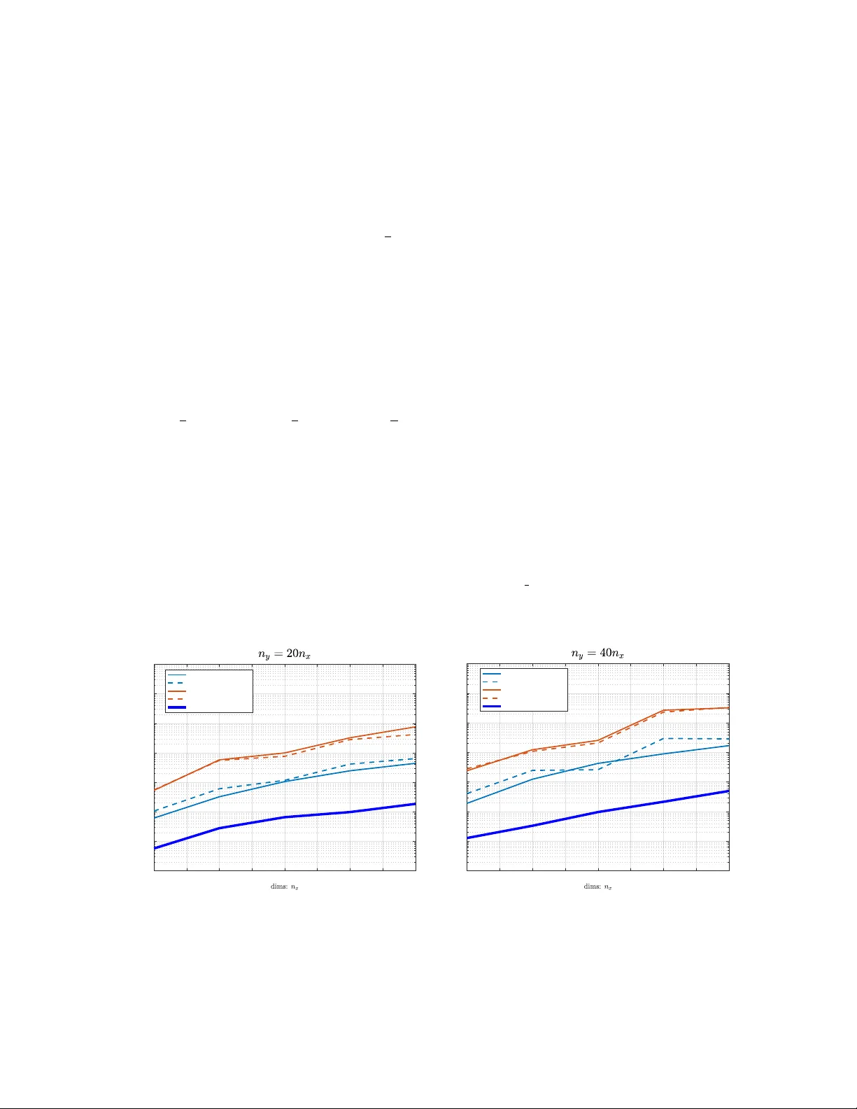
Proceedings of Machine Learning Research vol vvv: 1 – 13 , 2026 K oopman-BoxQP: Solving Large-Scale NMPC at kHz Rates Liang W u 1 W L I A N G 1 4 @ J H . E D U W allace Gian Y ion T an 2 W T G Y @ M I T . E D U Richard D. Braatz 2 B R A A T Z @ M I T . E D U J ´ an Drgo ˇ na 1 J D R G O NA 1 @ J H . E D U 1 Johns Hopkins University , MD 21218, USA 2 Massachusetts Institute of T echnolo gy , MA 02139, USA. Abstract Solving large-scale nonlinear model predictiv e control (NMPC) problems at kilohertz (kHz) rates on standard processors remains a formidable challenge. This paper proposes a K oopman-BoxQP framew ork that i) learns a linear K oopman high-dimensional model, ii) eliminates the high-dimensional observables to construct a multi-step prediction model of the states and control inputs, iii) penal- izes the multi-step prediction model into the objective, which results in a structured box-constrained quadratic program (BoxQP) whose decision v ariables include both the system states and control in- puts, iv) dev elops a structur e-e xploited and warm-starting-supported v ariant of the feasible Mehro- tra’ s interior-point algorithm for BoxQP . Numerical results demonstrate that K oopman-BoxQP can solve a lar ge-scale NMPC problem with 1040 v ariables and 2080 inequalities at a kHz rate. Keyw ords: Data-dri ven K oopman Operator, Nonlinear MPC, Quadratic Programming 1. Introduction Modern quadratic programming (QP) solvers ( Domahidi et al. , 2012 ; Ferreau et al. , 2014 ; Frison and Diehl , 2020 ; Zanelli et al. , 2020 ; W u and Bemporad , 2023 ) are able to solve small-scale linear MPC problems ( < 50 v ariables and < 100 inequalities) at kHz rates (milliseconds) on standard pro- cessors, but fail to achiev e similar performance for medium- or large-scale linear MPC problems (around 1000+ v ariables and 2000+ inequalities), let alone nonlinear programming-based nonlin- ear MPC problems (NMPC) ( Diehl et al. , 2009 ). Recently , data-dri ven K oopman approaches, which learn linear dynamics in a high-dimensional observ able space, ha ve emer ged as a computationally ef ficient way to transform NMPC problems into compact general QP formulations by eliminating the high-dimensional observ ables ( K orda and Mezi ´ c , 2018b ; Folk estad et al. , 2020 ). While existing Koopman-MPC frame works use the condensed MPC-to-QP construction ( Korda and Mezi ´ c , 2018b ) that only in volv es the control inputs (resulting in fe wer decision variables), the number of state inequality constraints can become v ery large when the state dimension is high, as is commonly the case in control of partial differential equations (PDEs) ( Arbabi et al. , 2018 ). As the computation times of QP solv ers typically depend on the total number of variables and inequal- ities , solving large-scale Koopman MPC problems at kHz rates using general-purpose QP solvers without exploiting problem structure remains computationally infeasible. Moreov er , for practical use, soft-constrained MPC formulations ( Zeilinger et al. , 2014 ) that introduce slack v ariables for state constraints to guarantee feasibility (at the expense of higher computational cost due to the increased number of variables) are commonly employed to handle unknown disturbances and mod- eling errors. Modeling errors are inevitable, as data-driv en finite-dimensional Koopman frameworks always in volv e projection and sampling errors ( Zhang et al. , 2022 ; Str ¨ asser et al. , 2025 ). © 2026 L. W u 1 , W .G.Y . T an 2 , R.D. Braatz 2 & J. Drgo ˇ na 1 . W U 1 T A N 2 B R A A T Z 2 D R G O ˇ N A 1 This article proposes a dynamics-relaxed alternativ e for K oopman-MPC problems, which penal- izes the approximated K oopman dynamic model via an ℓ 2 -penalty term in the objective, rather than embedding it into the inequality constraints as in condensed Koopman’ s MPC-to-QP construction ( K orda and Mezi ´ c , 2018b ). The proposed dynamics-relaxed K oopman-MPC approach can be re- garded as a sparse K oopman’ s MPC-to-QP construction, as the states are retained, while eliminating the high-dimensional observables in the offline phase. Unlike the condensed formulation in Korda and Mezi ´ c ( 2018b ), which yields a general QP , the proposed dynamics-relax ed K oopman-MPC for- mulation results in a structured box-constrained QP (BoxQP). T o tackle this problem efficiently , this article de velops a structur e-exploited and warm-starting-supported (note that the warm-starting does not w ork in IPMs for general QPs) Mehrotra’ s predictor–corrector interior point method (IPM) ( Mehrotra , 1992 ), which is capable of solving the resulting large-scale BoxQP at kHz rates. The ov erall framew ork is referred to as the K oopman-BoxQP solution for NMPC problems. 1.1. Contributions This article makes the following contributions, which are also the k ey factors as to ho w the proposed structure-exploited K oopman-BoxQP achiev es kHz-rate performance: 1) strictly feasible cold- and warm-start initializations are provided cost-free, enabling direct use of the feasible Mehrotra’ s predictor–corrector IPM algorithm; 2) the feasible Mehrotra IPM typically con verges to high-accuracy solutions of BoxQPs around 10 iterations (under strictly feasible cold-starts), regardless of the problem dimension, which is the ke y numerical finding highlighted in this article. Moreov er , warm-starting performs well in the feasible Mehrotra IPM for solving BoxQPs and in real-time MPC problems; warm-starting from pre vious solutions halves the iterations to about 6 ; 3) by exploiting structure, the dimension of the linear system solved in each IPM step is reduced from 5( n u + n x ) N p to n u N p , yielding substantial speedups (when n x ≫ n u , as in PDE control). 2. Problem F ormulation Nonlinear MPC: min N − 1 X k =1 ∥ x k +1 − x r ∥ 2 W x + ∥ u k − u r ∥ 2 W u (1a) + ∥ u k − u k − 1 ∥ 2 W ∆ u s.t. x 0 = x ( t ) , u − 1 = 0 , (1b) x k +1 = f ( x k , u k ) , k = 0 , . . . , N − 1 (1c) − 1 ≤ x k +1 ≤ 1 , k = 0 , . . . , N − 1 (1d) − 1 ≤ u k ≤ 1 , k = 0 , . . . , N − 1 (1e) This article considers a nonlinear MPC prob- lem (NMPC) for tracking, as shown in ( 1 ), where x ( t ) is the feedback state at the sam- pling time t , u k ∈ R n u and x k ∈ R n x denote the control input and state at the k th time step, the prediction horizon length is N , x r and u r denote the desired tracking reference signal for the state and control input, respec- ti vely , and W x ≻ 0 , W u ≻ 0 , and W ∆ u ≻ 0 are weighting matrices for the deviation of the state tracking error , control input track- ing error , and control input increment, re- specti vely . Assume that W x , W u , and W ∆ u are diagonal. The equality constraint ( 1c ) represents the nonlinear discrete-time dynamical system. W ithout loss of generality , the state and control input constraints, [ x min , x max ] and [ u min , u max ] , are scaled to [ − 1 , 1 ] . 2 K O O P M A N - B O X Q P NMPC ( 1 ) is a noncon vex nonlinear program, which can be infeasible, can be sensitive to the noise-contaminated x ( t ) , can hav e slow solving speed, and can lack of conv ergence guarantees. A K oopman framew ork for MPC ( K orda and Mezi ´ c , 2018b ), which transforms NMPC ( 1 ) into a con ve x QP problem via data-driven Koopman approximations, allows the use of computationally ef ficient and con ver gent QP algorithms for real-time applications. 3. Preliminary: K oopman transforms NMPC into general QP The K oopman operator ( Koopman , 1931 ; K oopman and Neumann , 1932 ) provides a globally linear representation of nonlinear dynamics, enabling efficient linear techniques for nonlinear systems. Originally dev eloped for autonomous systems, Koopman operator theory has since been extended to controlled systems of the form ( 1c ) through v arious schemes ( W illiams et al. , 2016 ; Proctor et al. , 2018 ; Korda and Mezi ´ c , 2018b ). In practice, the infinite-dimensional Koopman operator is truncated and approximated using data-driv en Extended Dynamic Mode Decomposition (EDMD) methods ( W illiams et al. , 2015 , 2016 ; K orda and Mezi ´ c , 2018a , b ). In EDMD specifically , the set of e xtended observ ables is designed as the “lifted” mapping,  ψ ( x ) u (0)  , where u (0) denotes the first component of the sequence u and ψ ( x ) ≜  ψ 1 ( x ) , · · · , ψ n ψ ( x )  ⊤ ( n ψ ≫ n x ) is chosen from a basis function, e.g., Radial Basis Functions (RBFs) used in Korda and Mezi ´ c ( 2018b ), instead of directly solving for them via optimization. In particular , the approximate Koopman operator identification problem is reduced to a least-squares problem, which assumes that the sampled data { ( x j , u j ) , ( x + j , u + j ) } (where j denotes the index of data samples and the superscript + denotes the v alue at the next time step) are collected with the update mapping  x + j u + j  =  f ( x j , u j (0)) S u j  . Then an approximation of the K oopman operator , A ≜ [ A B ] , can be obtained by solving J ( A, B ) = min A,B N d X j =1 ∥ ψ ( x + j ) − Aψ ( x j ) − B u j (0) ∥ 2 2 . (2) According to K orda and Mezi ´ c ( 2018b ), if the designed lifted mapping ψ ( x ) contains the state x after the re-ordering ψ ( x ) ← [ x ⊤ , ψ ( x )] ⊤ , then C = [ I , 0] . The learned linear Koopman predictor model is gi ven as ψ k +1 = Aψ k + B u k , x k +1 = C ψ k +1 , (3) where ψ k ≜ ψ ( x k ) ∈ R n ψ denotes the lifted state space and with ψ 0 = ψ ( x ( t )) . If ( 3 ) has a high lifted dimension (for a good approximation), its use in MPC will not increase the dimension of the resulting QP if the high-dimensional observ ables ψ k are eliminated via      x 1 x 2 . . . x N      = E ψ  x ( t )  + F      u 0 u 1 . . . u N − 1      , where E ≜      C A C A 2 . . . C A N      , F ≜      C B 0 · · · 0 C AB C B · · · 0 . . . . . . . . . . . . C A N − 1 B C A N − 2 B · · · C B      . (4) Then, by embedding ( 4 ) into the quadratic objectiv e ( 1a ) and the state constraint ( 1d ), NMPC ( 1 ) can be reduced to a compact general QP with the decision vector z ≜ col( u 0 , · · · , u N − 1 ) ∈ R N × n u as sho wn in ( 5 ), where ¯ W x ≜ blkdiag ( W x , · · · , W x ) , ¯ W u ≜ blkdiag ( W u , · · · , W u ) , ¯ R ≜ 3 W U 1 T A N 2 B R A A T Z 2 D R G O ˇ N A 1 blkdiag( ¯ W ∆ u , · · · , ¯ W ∆ u , ¯ W N ∆ u ) ¯ W ∆ u =  2 W ∆ u − W ∆ u − W ∆ u 2 W ∆ u  and ¯ W N ∆ u =  2 W ∆ u − W ∆ u − W ∆ u W ∆ u  ! and h ≜ F ⊤ ¯ W x ( E ψ ( x ( t )) − ¯ x r ) − ¯ W u ¯ u r ( ¯ x r = repmat( x r ) and ¯ u r = repmat( u r ) ). Note that the computation of the high-dimensional observable ψ ( x ( t )) is performed once and will not be inv olved in the iterations of QP , which minimizes a side effect of the high-dimensional Koopman operator . NMPC → Koopman-QP: min z z ⊤  F ⊤ ¯ W x F + ¯ W u + ¯ R  z + 2 z ⊤ h (5a) s.t. − 1 ≤ E ψ ( x t ) + F z ≤ 1 (5b) − 1 ≤ z ≤ 1 (5c) The resulting K oopman-QP ( 5 ) has N n u decision v ariables and 2 N ( n x + n u ) inequal- ity constraints, with no dependence on n ψ . The Koopman-QP ( 5 ) may be infeasible due to inevitable modeling errors in the data- dri ven Koopman appr oximation . By soften- ing the state constraints ( 5b ) to − 1 − ϵV min ≤ E ψ ( x t ) + F z ≤ 1 + ϵV max (the vectors V min and V max are non-positiv e) and adding a penalty term ρ ϵ ϵ 2 ( ρ ϵ ≫ W x , W u , W ∆ u ) to the objectiv e ( 5a ), then the K oopman-QP ( 5 ) with the new decision vector z ← col( z , ϵ ) is guaranteed to be feasible. Moreover , the K oopman-QP ( 5 ) constructed via condensing is a general QP without a specific structure, yet no existing work has de veloped a tailored structure-e xploited QP solver for the Koopman-MPC frame work to enable faster real-time computation. 4. Methodology T o simultaneously handle potential infeasibility and obtain faster execution time, this article pro- poses a dynamics-r elaxed construction that transforms the K oopman-MPC problem into a paramet- ric BoxQP , which is not al ways feasible but is guaranteed to be Lipschitz. The most important reason for choosing the construction is that we can customize a structure-e xploited and warm- starting-supported IPM-based QP solver to solve the QP at kHz rates, which general QPs cannot do, as demonstrated in Subsection 4.2 . 4.1. Koopman-BoxQP: Dynamics-r elaxed Construction Nonlinear MPC → Koopman-Bo xQP min U,X ( X − ¯ x r ) ⊤ ¯ W x ( X − ¯ x r ) + ( U − ¯ u r ) ⊤ ¯ W u ( U − ¯ u r ) + U ⊤ ¯ RU + ρ ∥ X − E ψ  x ( t )  − F U ∥ 2 2 s.t. − 1 ≤ U ≤ 1 , − 1 ≤ X ≤ 1 (6) This article proposes an alternativ e, the dynamic relaxation approac h , which does not strictly enforce the K oopman predic- tion model ( 4 ) but instead incorporates it into the objecti ve through a penalty term, which results in a strongly con vex BoxQP ( 6 ), where U ≜ col( u 0 , · · · , u N − 1 ) , X ≜ col( x 1 , · · · , x N ) , and ρ > 0 is a large penalty parameter reflecting the confidence in the K oopman model’ s accuracy . min z 1 2 z ⊤ H z + z ⊤ h ( x ( t )) s.t. − 1 ≤ z ≤ 1 (7) For simplicity , we denote the decision vector z ≜ col( U, X ) ∈ R n ( n = N ( n u + n x ) ), and the proposed 4 K O O P M A N - B O X Q P K oopman-BoxQP ( 6 ) is constructed as sho wn in ( 7 ), where H ≜ ρ  F ⊤ F − F ⊤ − F I  +  ¯ W u + ¯ R ¯ W x  ≻ 0 , h ( x ( t )) ≜ ρ  F ⊤ E − E  ψ ( x ( t )) −  ¯ W u ¯ u r ¯ W x ¯ x r  . (8) The dynamics-relax ed K oopman-BoxQP ( 6 ) can be viewed as an alternativ e approach to softening the state constraints, since the error in satisfying the prediction model can be equi valently interpreted as a relaxation of the state constraints. The dynamics-relaxed K oopman-BoxQP ( 6 ) is a parametric optimization, which is prov ed be- lo w to be feasible and hav e a Lipschitz-continuous feedback policy . The former property prev ents solver failure, and the latter property av oids chattering or abrupt control actions. Future work will le verage the prov en Lipschitz constant of the parametric BoxQP , incorporating that of the K oopman observ able, to certify the robustness of K oopman-MPC solutions ( T eichrib and Darup , 2023 ). Remark 1 ( F easibility-guaranteed ) The dynamics-r elaxed K oopman-BoxQP ( 6 ) (or ( 7 ) ) always admits a unique solution due to con vexity and non-empty constraints, thus guar anteeing feasibility . Lemma 2 ( Lipschitz-guaranteed ) Assume that the lifted mapping ψ ( · ) is Lipschitz continuous with constant L ψ . The feedback policy of K oopman-BoxQP ( 6 ) , u 0 ( x ( t )) ≜ C policy z ∗ ( x ( t )) , (9) wher e C policy = [ I n u , 0] ), is Lipschitz continuous with constant ρ √ λ max ( E ⊤ ( FF ⊤ + I ) E ) L ψ λ min ( H ) . Proof The optimal solution z ∗ ( x ( t )) can be characterized by the variational inequality:  H z ∗ ( x ( t )) + h ( x ( t ))  ⊤  z − z ∗ ( x ( t ))  , ∀ z ∈ [ − 1 , 1 ] . (10) Let us take x ( t 1 ) , x ( t 2 ) with corresponding solutions z 1 ≜ z ∗ ( x ( t 1 )) , z 2 ≜ z ∗ ( x ( t 2 )) and define ∆ h ≜ h ( x ( t 2 )) − h ( x ( t 1 )) , ∆ z ≜ z 2 − z 1 , ∆ x ≜ x ( t 2 ) − x ( t 1 ) . Applying ( 10 ) at each solution— for z 1 : ( H z 1 + h ( x ( t 1 ))) ⊤ ( z 2 − z 1 ) ≥ 0 , for z 2 : ( H z 2 + h ( x ( t 2 ))) ⊤ ( z 1 − z 2 ) ≥ 0 —and then adding the two inequalities results in ( H z 1 + h ( x ( t 1 ))) ⊤ ( z 2 − z 1 ) + ( H z 2 + h ( x ( t 2 ))) ⊤ ( z 1 − z 2 ) ≥ 0 , that is, ∆ z ⊤ H ∆ z ≤ − ∆ z ⊤ ∆ h . H ≻ 0 implies the strong con ve xity inequality λ min ( H ) ∥ ∆ z ∥ 2 2 ≤ ∆ z ⊤ H ∆ z . By the Cauchy-Schwarz inequality and the assumption, | ∆ z ⊤ ∆ h | ≤ ∥ ∆ z ∥ 2 ∥ ∆ h ∥ 2 and ∥ ∆ h ∥ 2 ≤ ρ ∥ [ F ⊤ E ; − E ] ∥ 2 L ψ ∥ ∆ x ∥ 2 = ρ q λ max ( E ⊤ ( FF ⊤ + I ) E ) L ψ ∥ ∆ x ∥ 2 . Combining those inequalities gi ves that λ min ( H ) ∥ ∆ z ∥ 2 2 ≤ ∥ ∆ z ∥ 2 ρ q λ max ( E ⊤ ( FF ⊤ + I ) E ) L ψ ∥ ∆ x ∥ 2 . That is, ∥ ∆ z ∥ 2 ≤ ρ √ λ max ( E ⊤ ( FF ⊤ + I ) E ) L ψ λ min ( H ) ∥ ∆ x ∥ 2 , namely , ∥ u 0 ( x ( t 2 )) − u 0 ( x ( t 1 )) ∥ 2 ≤ ∥ C policy ∥∥ ∆ z ∥ 2 ≤ ρ p λ max ( E ⊤ ( FF ⊤ + I ) E ) L ψ λ min ( H ) ∥ x ( t 2 ) − x ( t 1 ) ∥ 2 , which completes the proof. 5 W U 1 T A N 2 B R A A T Z 2 D R G O ˇ N A 1 4.2. Feasible Mehr otra’ s IPM Algorithm f or BoxQP KKT condition of BoxQP H z + h ( x ( t )) + γ − θ = 0 , (11a) z + ϕ − 1 n = 0 , (11b) z − ψ + 1 n = 0 , (11c) ( γ , θ , ϕ, ψ ) ≥ 0 , (11d) γ ⊙ ϕ = 0 , (11e) θ ⊙ ψ = 0 , (11f) According to Boyd and V andenberghe ( 2004 , Ch 5), the Karush–Kuhn–T ucker (KKT) condition of the BoxQP ( 7 ) is ( 11 ), where γ , θ are the Lagrangian variables of the lower and upper bound, respectiv ely; ϕ, ψ are the slack variables of the lower and upper bound, re- specti vely; ⊙ is the Hadamard product, i.e., γ ⊙ ϕ = col( γ 1 ϕ 1 , γ 2 ϕ 2 , · · · , γ n ϕ n ) . The BoxQP ( 7 ) may be ill- conditioned since the penalty parameter ρ needs to be large to ensure strong closed-loop performance. T o ad- dress this issue, this article employs second-order IPMs, with a particular focus on the most computationally ef ficient variant: Mehrotra’ s predictor–corrector IPM ( Mehrotra , 1992 ). In practice, Mehrotra’ s predictor–corrector IPM typically achie ves highly ac- curate solutions within 50 ∼ 75 iterations, regardless of whether the initial point is strictly feasible. This remarkably fast con ver gence makes the method the foundation of most IPM software packages. An important numerical observation in this article is that Mehrotra’ s predictor–corrector IPM typically takes about 10 iterations to find a highly accurate solution of BoxQP ( 7 ) when applying the following cost-free initialization strategy . T o demonstrate this, denote the feasible region by F , i.e., F = { ( z , γ , θ , ϕ, ψ ) : ( 11a ) − ( 11c ) , ( γ , θ , ϕ, ψ ) ≥ 0 } and the set of strictly feasible points by F + ≜ { ( z , γ , θ , ϕ, ψ ) : ( 11a ) − ( 11c ) , ( γ , θ , ϕ, ψ ) > 0 } . For a point ∈ F + , the residuals of ( 11a )–( 11c ) are zeros and only the residuals of the complementary equations ( 11e )–( 11f ) are not. 4.3. Cost-free strictly feasible cold- and warm-starting initializations IPMs for general optimization problems, including QPs, generally do not support warm-start initial- ization, which is an unfortunate limitation as warm-start initialization can substantially accelerate con ver gence and reduce iteration counts in real-time MPC applications. A notable advantage of the proposed K oopman-BoxQP ( 6 ) is its ability to support strictly feasible cold- and warm-start initializations without any e xtra computational ov erhead. Remark 3 ( Strictly feasible cold-start ): Inspir ed fr om ( W u and Braatz , 2025a , b ), the initial point ( z 0 , γ 0 , θ 0 , ϕ 0 , ψ 0 ) = (0 , ∥ h ( x ( t )) ∥ ∞ 1 n − 1 2 h ( x ( t )) , ∥ h ( x ( t )) ∥ ∞ 1 n + 1 2 h ( x ( t )) , 1 n , 1 n ) ∈ F + . (12) Remark 4 ( Strictly feasible warm-start ): The optimal solution at the pr evious sampling time t − 1 : U t − 1 = col( u t − 1 0 , · · · , u t − 1 N − 1 ) , X t − 1 = col( x t − 1 1 , · · · , x t − 1 N ) , can be shifted ahead one step to obtain a warm start initial point: z t, guess ≜ col( u t − 1 1 , · · · , u t − 1 N − 1 , u t − 1 N − 1 , x t − 1 2 , · · · , x t − 1 N , x t − 1 N ) (Clearly , − 1 n ≤ z t, guess ≤ 1 n ) to be used in solving the K oopman-BoxQP ( 6 ) at the curr ent sampling time t . The warm start initial point is z 0 = z t, guess , γ 0 = ∥ ¯ h ∥ ∞ 1 n − 1 2 ¯ h, θ 0 = ∥ ¯ h ∥ ∞ 1 n + 1 2 ¯ h, ϕ 0 = 1 n − z t, guess , ψ 0 = 1 n + z t, guess , (13) wher e ¯ h ≜ H z t, guess + h ( x ( t )) . Notably , we have ( z 0 , γ 0 , θ 0 , ϕ 0 , ψ 0 ) ∈ F + . 6 K O O P M A N - B O X Q P 4.4. Algorithm description and efficient computation of Newton systems Algorithm 1 Feasible Mehrotra’ s predictor- corrector IPM for BoxQP ( 7 ) Input : Initializing ( z 0 , γ 0 , θ 0 , ϕ 0 , ψ 0 ) from Eqn. ( 12 ), a desired optimal lev el ϵ , and the maximum number of iterations N max . for k = 0 , 1 , 2 , · · · , N max − 1 do 1. µ k ← [( γ k ) ⊤ ϕ k + ( θ k ) ⊤ ψ k ] / (2 n ) ; 2. if µ k ≤ (2 n ) ϵ , then break; 3. Compute (∆ z aff , ∆ γ aff , ∆ θ aff , ∆ ϕ aff , ∆ ψ aff ) by solving J k       ∆ z aff ∆ γ aff ∆ θ aff ∆ ϕ aff ∆ ψ aff       =       0 0 0 − γ k ⊙ ϕ k − θ k ⊙ ψ k       (14) where J k ≜       H I − I 0 0 I 0 0 I 0 I 0 0 0 − I 0 D ( ϕ k ) 0 D ( γ k ) 0 0 0 D ( ψ k ) 0 D ( θ k )       (15) 4. α aff = min(1 , 0 . 99 min ∆ γ aff i < 0 − γ k i ∆ γ aff i , 0 . 99 min ∆ θ aff i < 0 − θ k i ∆ θ aff i , 0 . 99 min ∆ ϕ aff i < 0 − ϕ k i ∆ ϕ aff i , 0 . 99 min ∆ ψ aff i < 0 − ψ k i ∆ ψ aff i ) ; 5. µ aff = [( γ k + α aff ∆ γ aff ) ⊤ ( ϕ k + α aff ∆ ϕ aff )+( θ k + α aff ∆ θ aff ) ⊤ ( ψ k + α aff ∆ ψ aff )] / (2 n ) ; 6. σ ←  µ aff µ k  3 ; 7. Compute (∆ z , ∆ γ , ∆ θ, ∆ ϕ, ∆ ψ ) by solving J k      ∆ z ∆ γ ∆ θ ∆ ϕ ∆ ψ      =       0 0 0 − γ k ⊙ ϕ k − ∆ γ aff ⊙ ∆ ϕ aff + σ µ k 1 n − θ k ⊙ ψ k − ∆ θ aff ⊙ ∆ ψ aff + σ µ k 1 n       (16) 8. α = min(1 , 0 . 99 min ∆ γ i < 0 − γ k i ∆ γ i , 0 . 99 min ∆ θ i < 0 − θ k i ∆ θ i , 0 . 99 min ∆ ϕ i < 0 − ϕ k i ∆ ϕ i , 0 . 99 min ∆ ψ i < 0 − ψ k i ∆ ψ i ) ; 9. z k +1 ← z k + α ∆ z, ← γ k + α ∆ γ , ← θ k + α ∆ θ, ← ϕ k + α ∆ ϕ, ψ k +1 ← ψ k + α ∆ ψ ; end Output: z k +1 . Algorithm 1 presents a feasible v ariant of Mehrotra’ s pre- dictor–corrector IPM, specifically tailored for BoxQP ( 7 ). At each iteration, Steps 3 and 4 of Algorithm 1 compute the predictor and corrector directions, respectiv ely , using the same coef ficient matrix J k ; thus, only a single ma- trix factorization is required. Moreov er , the structured sparsity of J k enables a more computationally ef ficient Cholesky factorization on a reduced-dimensional linear system, from 5 N × ( n u + n x ) → N × n u . Consider- ing ( 14 ) and ( 16 ), which dif fer only in the last two terms on the right-hand side, denote these terms as r 1 and r 2 , respecti vely . Then, by letting ∆ γ = γ k ϕ k ∆ z + r 1 ϕ k , ∆ θ = − θ k ψ k ∆ z + r 2 ψ k , ∆ ϕ = − ∆ z , ∆ ψ = ∆ z , (17) Equation ( 14 ) (or ( 16 )) can be reduced to a more compact system of linear equations, ¯ H ∆ z = r 1 ϕ − r 2 ψ , (18) where the coef ficient matrix ¯ H has a 2 × 2 block structure from the definition of H in ( 8 ): ¯ H ≜ H + D  γ k ϕ k + θ k ψ k  =  ¯ H 11 − ρ F ⊤ − ρ F ¯ H 22  ≻ 0 (19) (where D ( · ) denotes the diagonal matrix of a v ector) with ¯ H 11 ≜ ρ F ⊤ F + ¯ W u + ¯ R + D γ k 1: n 1 ϕ k 1: n 1 + θ k 1: n 1 ψ k 1: n 1 ! ¯ H 22 ≜ ρI + ¯ W x + D γ k n 1 +1: n ϕ k n 1 +1: n + θ k n 1 +1: n ψ k n 1 +1: n ! where ¯ H 11 ≻ 0 ∈ R n 1 × n 1 , ¯ H 22 ≻ 0 ∈ R n 2 × n 2 , n 1 = N n u , and n 2 = N n x . By assumption the weight- ing matrix W x is diagonal, thus ¯ W x and ¯ H 22 are also di- agonal. By exploiting the diagonal structure of ¯ H 22 , com- putational savings in solving ( 18 ) can be achie ved through solving the system:  ¯ H 11 − ρ 2 F ⊤ ¯ H − 1 22 F  ∆ z 1: n 1 = r 1 1: n 1 ϕ k 1: n 1 − r 2 1: n 1 ψ k 1: n 1 + ρ F ⊤ ¯ H − 1 22 r 1 n 1 +1: n ϕ k n 1 +1: n − r 2 n 1 +1: n ψ k n 1 +1: n ! (20) 7 W U 1 T A N 2 B R A A T Z 2 D R G O ˇ N A 1 and ∆ z n 1 +1: n = ¯ H − 1 22  r 1 n 1 +1: n ϕ k n 1 +1: n − r 2 n 1 +1: n ψ k n 1 +1: n + ρ F ∆ z 1: n 1  to obtain the solution ∆ z = col(∆ z 1: n 1 , ∆ z n 1 +1: n ) . Remark 5 By the Schur Complement lemma, ¯ H 11 − ρ 2 F ⊤ ¯ H − 1 22 F ≻ 0 , and the matrix is symmetric. Then, the Cholesky factorization with the cost O (( N n u ) 3 ) for ( 20 ) can be applied, which is crucial for achie ving computational speedup. 5. Numerical Examples 5.1. Practical behavior of cold-starting Mehr otra’ s IPM algorithm on random BoxQPs 200 400 600 800 1000 1200 1400 1600 1800 2000 Problem dimension: n 0 2 4 6 8 10 12 14 16 18 20 Number of iterations Feasible mean Infeasible mean Figure 1: Iteration counts of feasible and infeasi- ble Mehrotra’ s IPM algorithms on ill-conditioned random BoxQP problems with dimensions rang- ing from 100 to 2000 . The main inspiration for using the Koopman- BoxQP formulation comes from our con- tributed numerical observ ation as follows, F easible Mehr otra’ s IPM algo- rithm usually takes ∼ 10 itera- tions on (ill-conditioned) random BoxQP pr oblems, r e gar dless of the pr oblem dimension. T o verify this observation, we generate random BoxQP problems with dimensions n ranging from 100 to 2000 , where the Hessian matrix has a condition number of 10 6 . Algorithm 1 , with the desired optimality tolerance set ϵ = 10 − 6 , is applied both with and without the cold-start initialization strategy , corresponding to the fea- sible and infeasible variants, respectiv ely , for solving the generated BoxQP instances. For each specified problem dimension, the BoxQP is randomly generated and solved 100 times to char- acterize the statistical behavior of the iteration counts of feasible and infeasible Mehrotra’ s IPM algorithms, which are plotted in Fig. 1 . Clearly , Fig. 1 confirms our key numerical observ ation: the feasible Mehrotra’ s IPM algorithm (Algorithm 1 ) is scalable , requiring only about 10 iterations to achie ve highly accurate solutions. 5.2. Perf ormance validation of K oopman-BoxQP on PDE NMPC pr oblems This section applies our proposed Koopman-BoxQP to solve a PDE-MPC problem with state and control input constraints, which is a large-sized QP problem with 1040 variables and 2080 con- straints. The PDE plant under consideration is the nonlinear Korte weg-de Vries (KdV) equation that models the propagation of acoustic wa ves in plasma or shallo w water wav es ( Miura , 1976 ) as ∂ y ( t, x ) ∂ t + y ( t, x ) ∂ y ( t, x ) ∂ x + ∂ 3 y ( t, x ) ∂ x 3 = u ( t, x ) (21) where x ∈ [ − π , π ] is the spatial variable. Consider the control input u ( t, x ) = P 4 i =1 u i ( t ) v i ( x ) , in which the four coefficients { u i ( t ) } are subject to the constraint [ − 1 , 1] , and v i ( x ) are predetermined 8 K O O P M A N - B O X Q P spatial profiles giv en as v i ( x ) = e − 25( x − m i ) 2 , with m 1 = − π / 2 , m 2 = − π / 6 , m 3 = π / 6 , and m 4 = π / 2 . The control objecti ve is to adjust u i ( t ) so that the spatial profile y ( t, x ) tracks the given reference signal. The spatial profile y ( t, x ) is uniformly discretized into 100 spatial nodes. These 100 discretized nodes serve as the system states, each constrained within [ − 1 , 1] , while the control inputs are likewise bounded within [ − 1 , 1] . Choosing the MPC prediction horizon as N = 10 results in a medium-scale optimization problem with 1040 variables and 2080 constraints. For the MPC settings, the state cost matrix is set to W x = I 100 , and the control inputs matrix is set to W u = 0 . 05 I 4 . The state references x r ∈ R 100 are sinusoidal signals for a 50 s simulation time, and the control input reference is a constant value with u r = 0 . W e employ a spectral method based on the Fourier transform and a split-step scheme to solve the nonlinear KdV ( 21 ), for data generation and MPC closed-loop simulation. The sampling time is chosen to be ∆ t = 0 . 01 . 0 10 20 30 40 50 60 70 80 0 2 4 6 8 10 12 14 16 18 20 Number of Iterations Figure 2: Iterations comparison of Algorithm 1 with Cold-start and W arm-start. QP Solver A verage Execution T ime [s] 1 cold start warm start Quadprog 0.1127 0.1127 OSQP 9 . 7 × 10 − 3 1 . 2 × 10 − 3 SCS 5 . 8 × 10 − 3 5 . 8 × 10 − 3 Algorithm 1 5 . 57 × 10 − 4 3 . 63 × 10 − 4 T able 1: Execution time comparison between Al- gorithm 1 and other state-of-the-art QP solvers. The setting for our closed-loop simulation includes: (i) Data gener ation: The data are col- lected from 1000 simulation trajectories with 200 samples. At each simulation, the ini- tial condition of the spatial profile is a ran- dom combination of four given spatial pro- files, i.e., y 0 1 (0 , x ) = e − ( x − π / 2) 2 , y 0 2 (0 , x ) = − sin( x/ 2) 2 , y 0 3 (0 , x ) = e − ( x + π / 2) 2 , y 0 4 (0 , x ) = cos( x/ 2) 2 . The four control inputs u i ( t ) are distributed uniformly in [ − 1 , 1] ; (ii) K oopman pr edictor: The lift function ψ is composed of the original 100 spatial states and 200 thin-plate RBFs with random centers, which leads to the lifted state dimension N ψ = 100 + 200 = 300 . Then the lifted linear predictor with A ∈ R 300 × 300 and B ∈ R 300 × 4 is obtained from the Moore-Penrose pseudoin verse of the lift- ing data matrix, and its output matrix is C = [ I 100 , 0] ∈ R 100 × 300 ; (iii) K oopman-BoxQP formulation: Giv en the matrices { A, B , C } cal- culated from the above pre vious K oopman pre- dictor step, the approximated multi-step Koop- man model ( 4 ) is constructed and embedded into the Koopman-BoxQP ( 6 ) with dynamic penalty parameter ρ = 10 2 . This results in a BoxQP with 1040 variables and 2080 con- straints. The proposed Algorithm 1 with the stop- ping criteria ϵ = 1 × 10 − 6 is applied to solve the resulting large-size K oopman-BoxQP problem ( 6 ) in the closed-loop simulation. The closed-loop performance, shown in Fig. 3 , demonstrates that the spatial profile y ( t, x ) accurately tracks the desired reference signals while remaining within the state constraint [ − 1 , 1] , ev en when the reference signals exceed this bound. The control inputs 1. The execution time results are based on MA TLAB’ s C-MEX implementation of Algorithm 1 running on a Mac mini with an Apple M4 Chip (10-core CPU and 16 GB RAM). 9 W U 1 T A N 2 B R A A T Z 2 D R G O ˇ N A 1 also remain strictly within their limits of [ − 1 , 1] . This numerical case study demonstrates that the proposed K oopman-BoxQP approach can accurately control the e volution of lar ge-scale states. Figure 3: Closed-loop simulation of the nonlinear KdV system with the dynamics-relaxed K oopman-BoxQP controller tracking a time-varying spatial profile reference. Left: time ev olution of the spatial profile y ( t, x ) and the state constraints [ − 1 , 1] . Middle: spatial mean of the y ( t, x ) and the state constraints [ − 1 , 1] . Right: the four control inputs and the control input constraints [ − 1 , 1] . The number of iterations of the IPM-based Algorithm 1 with cold and warm starts is plotted in Fig. 2 , which demonstrates that Algorithm 1 ef fectively supports warm-start initialization, reducing the average number of iterations by half, from 11 . 2039 (cold start) to 6 . 4745 (warm start). This implies that solving around 6 small-scale linear systems (reduced from large-scale via exploiting the problem structure) can obtain 10 − 6 -accuracy solutions, explaining why Algorithm 1 can solve lar ge-scale NMPC pr oblems at kHz rates (in milliseconds) as shown in T able 1 . Other state-of- the-art QP solvers, including MA TLAB’ s Quadprog (using IPM), OSQP ( Stellato et al. , 2020 ), and SCS ( O’Donoghue , 2021 ) (all choose the ‘eps rel’, ‘1e-6’ for a fair comparison), are compared for solving the same resulting K oopman-BoxQP ( 6 ). Their av erage ex ecution times under cold- and warm-start initialization are listed in T able 1 , which shows that using a warm start is not helpful in the IPM-based solvers Quadprog and SCS, but beneficial in Algorithm 1 . Furthermore, Algorithm 1 is the only solv er that achie ves kHz-le vel solution speeds for large-scale NMPC problems. More- ov er , the proposed Algorithm 1 has been extended to general QPs, and more numerical experiments can be found in the Appendix A due to space limits. 6. Conclusion This article presents a fast K oopman-BoxQP framew ork enabling NMPC at kHz rates. Our ap- proach consists of a dynamics-r elaxed BoxQP formulation and a linear -algebr a-tailor ed and warm- starting-supported IPM-based QP solver . W e validated the approach on a challenging large-sized PDE-MPC problem (with 1040 decision variables and 2080 inequality constraints) and achiev ed a real-time solution under < 1 ms on a standard desktop CPU, opening a new era of kHz-rate solutions for large-scale NMPC. Future work will focus on dev eloping a GPU-accelerated Koopman-BoxQP solver , lev eraging the computational power of cuBLAS and cuSOL VER for large-scale linear sys- tem solves, together with the practical scalable iteration comple xity (typically around 10 iterations) of the IPM in BoxQPs, to enable larger PDE-MPC applications. The stability proof and robustness of the dynamics-r elaxed K oopman-BoxQP will also be in vestigated. 10 K O O P M A N - B O X Q P Acknowledgments This research was supported by the Ralph O’Connor Sustainable Ener gy Institute at Johns Hopkins Uni versity . W allace T an was supported by the MathW orks Fellowship. Richard Braatz was sup- ported by the U.S. Food and Drug Administration under the FD A B AA-22-00123 program (A ward 75F40122C00200). References Hassan Arbabi, Milan K orda, and Igor Mezi ´ c. A Data-Driven Koopman Model Predictiv e Control Frame work for Nonlinear Partial Differential Equations. In IEEE Confer ence on Decision and Contr ol , pages 6409–6414, 2018. Stephen P . Boyd and Liev en V andenberghe. Con ve x Optimization . Cambridge Univ ersity Press, U.K., 2004. Moritz Diehl, Hans Joachim Ferreau, and Niels Hav erbeke. Efficient numerical methods for nonlin- ear MPC and moving horizon estimation. In Nonlinear Model Pr edictive contr ol: T owar ds New Challenging Applications , pages 391–417. Springer V erlag, 2009. Alexander Domahidi, Aldo U. Zgraggen, Melanie N. Zeilinger , Manfred Morari, and Colin N. Jones. Efficient interior point methods for multistage problems arising in receding horizon con- trol. In IEEE 51st IEEE Confer ence on Decision and Contr ol , pages 668–674, 2012. Hans Joachim Ferreau, Christian Kirches, Andreas Potschka, Hans Georg Bock, and Moritz Diehl. qpO ASES: A parametric activ e-set algorithm for quadratic programming. Mathematical Pr o- gramming Computation , 6(4):327–363, 2014. Carl Folk estad, Daniel Pastor , Igor Mezic, Ryan Mohr, Maria Fonoberov a, and Joel Burdick. Ex- tended Dynamic Mode Decomposition with Learned Koopman Eigenfunctions for Prediction and Control. In American Contr ol Confer ence , pages 3906–3913, 2020. Gianluca Frison and Moritz Diehl. HPIPM: A high-performance quadratic programming framework for model predicti ve control. IF AC-P apersOnLine , 53(2):6563–6569, 2020. Bernard O. Koopman. Hamiltonian systems and transformation in Hilbert space. Pr oceedings of the National Academy of Sciences , 17(5):315–318, 1931. Bernard O. K oopman and J. V . Neumann. Dynamical systems of continuous spectra. Pr oceedings of the National Academy of Sciences , 18(3):255–263, 1932. Milan Korda and Igor Mezi ´ c. On con ver gence of extended dynamic mode decomposition to the Koopman operator . Journal of Nonlinear Science , 28(2):687–710, 2018a. Milan Korda and Igor Mezi ´ c. Linear predictors for nonlinear dynamical systems: Koopman operator meets model predicti ve control. Automatica , 93:149–160, 2018b. Sanjay Mehrotra. On the implementation of a primal-dual interior point method. SIAM J ournal on Optimization , 2(4):575–601, 1992. 11 W U 1 T A N 2 B R A A T Z 2 D R G O ˇ N A 1 Robert M. Miura. The Korteweg–deVries equation: A survey of results. SIAM Review , 18(3): 412–459, 1976. Brendan O’Donoghue. Operator Splitting for a Homogeneous Embedding of the Linear Comple- mentarity Problem. SIAM Journal on Optimization , 31:1999–2023, 2021. Joshua L. Proctor , Stev en L. Brunton, and J. Nathan Kutz. Generalizing Koopman theory to allow for inputs and control. SIAM Journal on Applied Dynamical Systems , 17(1):909–930, 2018. Bartolomeo Stellato, Goran Banjac, Paul Goulart, Alberto Bemporad, and Stephen Boyd. OSQP: An operator splitting solver for quadratic programs. Mathematical Pr ogramming Computation , 12(4):637–672, 2020. Robin Str ¨ asser , Manuel Schaller, Julian Berberich, Karl W orthmann, and Frank Allg ¨ ower . K ernel- based error bounds of bilinear Koopman surrogate models for nonlinear data-dri ven control. arXiv pr eprint arXiv:2503.13407 , 2025. Dieter T eichrib and Moritz Schulze Darup. Ef ficient computation of Lipschitz constants for MPC with symmetries. In 62nd IEEE Confer ence on Decision and Contr ol , pages 6685–6691, 2023. Matthe w O. Williams, Ioannis G. Ke vrekidis, and Clarence W . Rowle y . A data-driven approxima- tion of the Koopman operator: Extending dynamic mode decomposition. Journal of Nonlinear Science , 25(6):1307–1346, 2015. Matthe w O. W illiams, Maziar S. Hemati, Scott T . M. Dawson, Ioannis G. Ke vrekidis, and Clarence W . Rowle y . Extending data-driv en K oopman analysis to actuated systems. IF AC- P apersOnLine , 49(18):704–709, 2016. Liang W u and Alberto Bemporad. A Simple and Fast Coordinate-Descent Augmented-Lagrangian Solver for Model Predictiv e control. IEEE T ransactions on Automatic Contr ol , 68(11):6860– 6866, 2023. Liang W u and Richard D. Braatz. A Direct Optimization Algorithm for Input-Constrained MPC. IEEE T ransactions on Automatic Contr ol , 70(2):1366–1373, 2025a. Liang W u and Richard D Braatz. A Quadratic Programming Algorithm with O ( n 3 ) Time Com- plexity . arXiv pr eprint arXiv:2507.04515 , 2025b. Andrea Zanelli, Ale xander Domahidi, Juan Jerez, and Manfred Morari. FORCES NLP: An ef- ficient implementation of interior-point methods for multistage nonlinear noncon ve x programs. International Journal of Contr ol , 93(1):13–29, 2020. Melanie N. Zeilinger , Manfred Morari, and Colin N. Jones. Soft constrained model predicti ve control with robust stability guarantees. IEEE T ransactions on Automatic Contr ol , 59(5):1190– 1202, 2014. Xinglong Zhang, W ei Pan, Riccardo Scattolini, Shuyou Y u, and Xin Xu. Robust tube-based model predicti ve control with Koopman operators. Automatica , 137:110114, 2022. 12 K O O P M A N - B O X Q P A ppendix A. Numerical experiments on general QPs The proposed BoxQP solver in the dynamics-relaxed K oopmanMPC-to-BoxQP approach can be extended to general QPs, not limited to nonlinear MPC applications. Consider a general con ve x QP , min x 1 2 x ⊤ Qx + q ⊤ x (22a) s.t. y min ≤ Ax ≤ y max (22b) x min ≤ x ≤ x max (22c) where x ∈ R n x , Q = Q ⊤ ⪰ 0 and Q ∈ R n x × n x , q ∈ R n x , and A ∈ R n y × n x . The bound con- straint ( 22c ) often comes from the physical actuator limits, and ( 22b ) comes from user-specified constraints, such as the states/outputs constraints. T o ensure feasibility without violating hard actu- ator limits, the core idea of this article is the use of the soft-constrained formulation as follo ws, min x,y 1 2 x ⊤ Qx + q ⊤ x + ρ 2 ∥ Ax − y ∥ 2 2 = 1 2  x y  ⊤  Q + ρA ⊤ A − ρA ⊤ − ρA ρI   x y  +  x y  ⊤  q 0  s.t.  x min y min  ≤  x y  ≤  x max y max  (23) where ρ is a large penalty parameter, such as ρ = 10 6 . The soft-constrained BoxQP ( 23 ) is always feasible, Lipschitz-guaranteed, and supports the lightening fast tailored solv er (from two reasons: i) only requiring roughly 10 iterations for a high-accuracy solution, ii) allowing the dimension reduc- tion of linear systems) especially when n y ≫ n x , such as from PDE-MPC applications. Algorithm 1 is compared ag ainst OSQP and SCS solvers (all choose the ‘eps rel’, ‘1e-6’) on random QPs ( 22 ), and Fig. 4 sho ws that Algorithm 1 is f astest (at least an order of magnitude f aster) and only requires roughly 10 − 2 s on QPs with 8400 inequalities. 40 60 80 100 120 140 160 180 200 10 -4 10 -3 10 -2 10 -1 10 0 10 1 10 2 10 3 Computation time [s] OSQP for standard (21) OSQP for soft (22) SCS for standard (22) SCS for soft (23) Algorithm 1 40 60 80 100 120 140 160 180 200 10 -4 10 -3 10 -2 10 -1 10 0 10 1 10 2 10 3 Computation time [s] OSQP for standard (21) OSQP for soft (22) SCS for standard (22) SCS for soft (23) Algorithm 1 Figure 4: Execution time comparison between Algorithm 1 , OSQP , and SCS solvers on random QPs (and their soft-constrained QPs with ρ = 10 6 ) with different dimensions. Left: n y = 20 n x . Right: n y = 40 n x . 13