Neural-HSS: Hierarchical Semi-Separable Neural PDE Solver

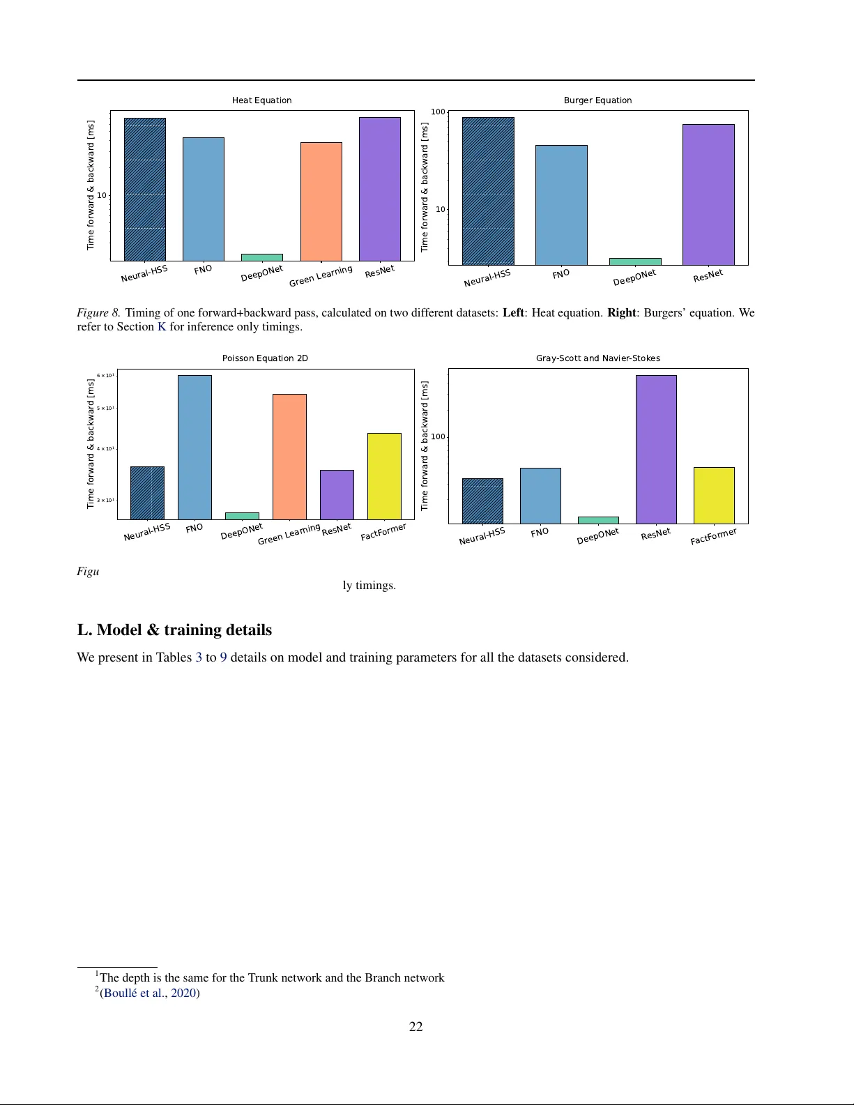
Neural-HSS: Hierar chical Semi-Separable Neural PDE Solver Pietro Sittoni * 1 Emanuele Zangrando * 1 Angelo Alberto Casulli 1 Nicola Guglielmi 1 Francesco T udisco 1 2 3 Abstract Deep learning-based methods hav e sho wn remark- able effecti v eness in solving PDEs, largely due to their ability to enable fast simulations once trained. Howe v er , despite the av ailability of high- performance computing infrastructure, many crit- ical applications remain constrained by the sub- stantial computational costs associated with gener- ating large-scale, high-quality datasets and train- ing models. In this work, inspired by studies on the structure of Green’ s functions for elliptic PDEs, we introduce Neural-HSS, a parameter- efﬁcient architecture built upon the Hierarchical Semi-Separable (HSS) matrix structure that is prov ably data-efﬁcient for a broad class of PDEs. W e theoretically analyze the proposed architec- ture, proving that it satisﬁes e xactness properties ev en in very low-data regimes. W e also inv esti- gate its connections with other architectural primi- ti ves, such as the Fourier neural operator layer and con volutional layers. W e experimentally validate the data efﬁciency of Neural-HSS on the three- dimensional Poisson equation o ver a grid of two million points, demonstrating its superior ability to learn from data generated by elliptic PDEs in the lo w-data regime while outperforming baseline methods. Finally , we demonstrate its capability to learn from data arising from a broad class of PDEs in di verse domains, including electromagnetism, ﬂuid dynamics, and biology . 1. Introduction and Related W ork Machine learning is emerging as a powerful tool for accu- rately simulating complex ph ysical phenomena ( Brandstet- ter et al. , 2022 ; Li et al. , 2021 ; Boullé et al. , 2023 ). Unlike traditional numerical methods, which rely on explicit math- ematical models and require problem-speciﬁc implementa- 1 Gran Sasso Science Institute, L ’Aquila, Italy . 2 Univ ersity of Edinbur gh, UK. 3 Miniml.AI. Correspondence to: Pietro Sittoni , Emanuele Zangrando . Pr eprint. F ebruary 23, 2026. tions for spatial resolution, timescales, domain geometry , and boundary conditions, machine learning models learn directly from data—either from simulations or real-world observations—enabling greater ﬂexibility and scalability . Moreov er , these models lev erage ongoing advances in GPU acceleration and large-scale parallelization, with continued improv ements in both accuracy and ef ﬁciency . A wide range of architectural primiti ves has been e xplored for modeling dif ferent physical systems, each leveraging structural biases that arise in the solution operator of spe- ciﬁc classes of PDEs. As prominent examples, the F ourier neural operator ( Li et al. , 2021 ) learns a kernel integral oper - ator through con volution in F ourier space, enabling efﬁcient representation of global interactions; message passing neu- ral networks ( Brandstetter et al. , 2022 ) capture localized interactions via graph-based message updates; U-Net Con- vNets ( Gupta & Brandstetter , 2022 ) exploit multiscale rep- resentations to couple ﬁne- and coarse-scale features; while operator transformers ( Hao et al. , 2023 ) lev erage transform- ers to handle challenging settings such as irregular meshes. Other methods directly approximate the action of linear operators in the elliptic setting ( Boullé et al. , 2023 ), by- passing explicit discretization of the underlying equations. Moreov er , ( Boullé et al. , 2023 ) show that the underlying learning problem is well-posed for a v ery small number of datapoints and prov e that the class of elliptic PDEs is “data efﬁcient”: the number of training points needed to learn the solution operator depends only on the problem dimension. This ef fect is due to the nature of the solution operator for elliptic-type PDEs, which is highly structured: the Green function G ( x, y ) associated with the solution operator is a Hierarchical Semi-Separable ( HSS ) mapping that e xhibits low rank when restricted to of f-diagonal subdomains. In fact, the Multipole Graph Neural Operator emplo yed in ( Boullé et al. , 2023 ) is motiv ated by a hierarchical struc- ture observed in Green functions ( Boullé & T ownsend , 2024 , Section 2.4), known as the Hierarchical Off-Diagonal Low-Rank (HODLR) structure. In an HODLR matrix, off- diagonal blocks at different scales are well-approximated by low-rank f actorizations. When used within a neural ar- chitecture, this ﬂexible representation allows the netw ork to capture both near-ﬁeld and far-ﬁeld interactions in a mul- tiscale fashion and is one of the key factors behind the data-efﬁcienc y property of the neural architecture. 1 Neural-HSS: Hierarchical Semi-Separable Neural PDE Solv er The HSS structure is a special case of the more general HODLR format, a hierarchical domain-decomposition strat- egy that has been widely studied in the scientiﬁc computing literature for de veloping f ast and memory-ef ﬁcient solv ers for elliptic-type PDEs, e.g., ( Martinsson & Rokhlin , 2005 ; Gillman et al. , 2012 ). Compared to HODLR, the HSS model enforces a nested basis across lev els in addition to low-rank off-diagonal blocks. This nested parameterization greatly reduces redundancy , yielding a more compact representa- tion and faster matrix–v ector products, improvements that are not av ailable in the plain HODLR structure. In this work, we propose Neural-HSS, a neural architecture that injects this type of structure into a neural netw ork model for PDE learning. Thanks to the ef ﬁcient data representation of HSS , the proposed model is able to approximate solution operators with far fewer parameters than baseline models while retaining better or comparable accuracy . The geometric structure of HSS operators imposes an in- ductiv e bias that concentrates modeling capacity on local interaction ef fects in the physical system—modeled through full-rank submatrices—while approximating interaction ef- fects between distant subdomains using lo w-rank matrices, resembling a mean-ﬁeld approximation. This modeling strategy underlies many popular neural PDE solvers. In fact, architectures such as ResNets ( He et al. , 2016 ), Swin T ransformers ( Liu et al. , 2021 ), and Message P assing Neu- ral Networks ( Gilmer et al. , 2017 ) dev ote the majority of their representational capacity to modeling local interactions. This bias aligns well with the nature of PDE dynamics, in which the dominant behavior is dri ven by localized interac- tions, in contrast to integro-differential equations, which can incorporate global interaction effects. The effect of this im- plicit bias was also highlighted in ( Holzschuh et al. , 2025 ), where the authors demonstrate that in a Swin-T ransformer- based model, increasing the attention windo w size leads to a rapid performance plateau. Overall, our main contrib utions are as follo ws: • W e propose Neural-HSS, a parameter -efﬁcient neural architecture with a nov el type of layer inspired by HSS theory for PDEs ( Hackbusch , 2015 ), and we establish its univ ersal approximation property . • W e prov e that the proposed architecture is exact and data-efﬁcient on the class of elliptic PDEs, i.e., (a) the global minimizers of the empirical loss represent the discretized solution operator exactly , and (b) the number of data points required to learn the exact op- erator depends only on the intrinsic dimensionality of the problem. T o the best of our knowledge, this is the ﬁrst result for an architecture that can handle arbitrary types of PDEs while guaranteeing exactness and data efﬁcienc y for a broad class of PDEs. • W e highlight an intriguing connection between the pro- posed architecture and a discretized version of the con volutional-type layer used in FNO architectures, showing that an HSS layer can approximate it arbitrar- ily well with very fe w parameters. • Under the assumptions of Theorem 2.3 , which match the setting of ( Boullé et al. , 2023 ), we conduct two experiments in 1 D and 3 D. The 3 D experiment is per - formed on a grid with 2 M points, a well-kno wn chal- lenge for machine learning models. In both cases, we demonstrate the superior performance and scalability of Neural-HSS. • W e conduct extensiv e experiments on a broad class of PDEs arising from electromagnetism, ﬂuid dynamics, and biology , sho wcasing strong performance relati ve to commonly used architectural primitiv es such as ResNet and FNO layers in terms of parameter efﬁcienc y , test error , and computational time. In particular , this last ad- vantage becomes more e vident for higher-dimensional PDEs. Moreover , we demonstrate the ef fecti veness of Neural-HSS beyond elliptic PDEs, showing that the same architecture is also ef fectiv e for different classes of nonlinear PDEs. Related W ork. There has been a surge of interest in learning-based approaches for impro ving classical solvers for linear PDEs. Sev eral works focus on accelerating iter- ativ e methods such as Conjugate Gradient for symmetric positiv e deﬁnite systems ( Li et al. , 2023a ; Kaneda et al. , 2023 ; Zhang et al. , 2023 ), or GMRES-type solvers for spe- ciﬁc applications like the Poisson equation ( Luna et al. , 2021 ). Others focus on learned preconditioning strategies: neural networks ha ve been used to construct precondition- ers that speed up con vergence ( Greenfeld et al. , 2019 ; Luz et al. , 2020 ; T aghibakhshi et al. , 2021 ), or to optimize heuris- tics such as Jacobi and ILU variants ( Flegar et al. , 2021 ; Stanaityte , 2020 ). NeurKItt ( Luo et al. , 2024 ), for example, employs a neural operator to predict the in variant subspace of the system matrix and accelerate solution con ver gence. Howe ver , these approaches are primarily designed to en- hance classical linear numerical pipelines. In contrast, our work takes a fundamentally different perspecti ve: we aim to learn an end-to-end solver . Moreov er , recent work has focused on learning lo w- dimensional latent re presentations of PDE states for efﬁcient simulation, extending classical projection-based reduction ( Benner et al. , 2015 ) with deep learning methods such as autoencoders ( Wie wel et al. , 2019 ; Maulik et al. , 2021 ), graph embeddings ( HAN et al. , 2022 ), and implicit neu- ral representations ( Chen et al. , 2022 ). Koopman-inspired methods enforce linear latent dynamics ( Genev a & Zabaras , 2022 ; Y eung et al. , 2019 ), while latent neural solvers and 2 Neural-HSS: Hierarchical Semi-Separable Neural PDE Solv er transformer-based R OMs ha ve been dev eloped for end-to- end modeling ( Li et al. , 2025a ; Hemmasian & Barati Fari- mani , 2023 ). In addition, ( Kissel & Diepold , 2023b ) intro- duces a hierarchical ( Fan et al. , 2019b ) network to model the nonlinear Schrödinger equation. Another key challenge remains long-horizon stability , motiv ating strategies like autoregressi ve training, architectural constraints, and spec- tral or stochastic re gularization ( Gene v a & Zabaras , 2020 ; McCabe et al. ; Stachenfeld et al. , 2022 ). More recently , gen- erativ e models, in particular using diffusion-based models, hav e sho wn promise for stable rollout and data assimilation by producing statistically consistent trajectories ( Shyshe ya et al. , 2024 ; Li et al. , 2025b ; Andry et al. , 2025 ). The use of structured matrices in neural network architec- tures is also highly rele v ant and used across dif ferent areas of deep learning. Recent approaches include the use of low-rank ( Schotthöfer et al. , 2022 ; Zangrando et al. , 2024 ) and hierarchical decompositions ( F an et al. , 2019a ; Kissel & Diepold , 2023a ), lo w-displacement rank ( Thomas et al. , 2019 ; Zhao et al. , 2017 ; Choromanski et al. , 2024 ), but- terﬂies and monarchs ( Fu et al. , 2023 ; Dao et al. , 2019 ; 2022 ). 2. Setting and Model In this section, we present the necessary deﬁnitions and theoretical motiv ations for our proposed architecture. W e start with the following formal deﬁnition of HSS structure: Deﬁnition 2.1. ( HSS structure ( Casulli et al. , 2024 , Deﬁni- tion 3.1)) Let T be a cluster tree of depth L for the indices [1 , . . . , d ] . A matrix A ∈ R d × d belongs to HSS ( r , T ) or simply HSS ( r ) if there exist real matrices { U τ , V τ : τ ∈ T , 1 ≤ depth( T ) } and { D τ : τ ∈ T } called telescopic decomposition and for bre vity denoted by { U τ , V τ , D τ } τ ∈T or simply { U τ , V τ , D τ } , with the follow- ing properties: 1. D τ is of size | τ | × | τ | if depth( τ ) = L and 2 r × 2 r otherwise; 2. U τ , V τ are of size | τ | × r if depth( τ ) = L and 2 r × r otherwise; 3. if L = 0 (i.e., T consists only of the root γ ) then A = D γ ; 4. if L ≥ 1 then A = D ( L ) + U ( L ) A ( L − 1) ( V ( L ) ) T where U ( L ) := blkdiag( U τ : τ ∈ T , depth( τ ) = L ) , V ( L ) := blkdiag( V τ : τ ∈ T , depth( τ ) = L ) , D ( L ) := blkdiag( D τ : τ ∈ T , depth( τ ) = L ) and the matrix A ( L − 1) := ( U ( L ) ) T ( A − D ( L ) ) V ( L ) has the telescopic decomposition { U τ , V τ , D τ } τ ∈T ( L − 1) 2 r , where T ( L − 1) 2 r denotes a balanced cluster tree of depth L − 1 for the indices [1 , . . . , 2 L r ] , see Theorem A.2 . This deﬁnition is a natural extension of the idea of a low- rank linear operator, when the matrix is not globally low- rank but admits a low-rank e xpansion on subdomains that do not intersect. The utility and efﬁcienc y of these structures become imme- diately clear when considering elliptic-type PDEs. In fact, when one discretizes an elliptic partial differential operator— say by ﬁnite differences, ﬁnite elements, or boundary in- tegral methods—a large algebraic system Au = f arises, where A is associated with discretized Green’ s functions. It turns out that many of the of f-diagonal blocks of A hav e low numerical rank because of the smoothing properties of elliptic operators, making distant interactions "weak" and therefore inducing a decay in the singular values, which depends on the regularity of the kernel ( Bebendorf , 2000 ; Bebendorf & Hackb usch , 2003 ). HSS matrices exploit ex- actly this feature by or ganizing the matrix into a hierarchical block structure in which off-diagonal blocks are approxi- mated by low-rank f actorizations. Thus, HSS-based models are used to design fast numerical solvers or preconditioners for elliptic PDEs by efﬁciently approximating the opera- tor , thereby reducing storage and computational complexity ( Börm , 2010 ; Börm & Grasedyck , 2005 ; Gillman et al. , 2012 ). As the HSS structure is in variant under matrix in- version, these properties demonstrate that HSS operators can ef fecti vely model the structure of the solution operator and of fer a po werful modeling primiti ve for a neural PDE solver . Based on this key observation, we propose below the Neural- HSS model. 2.1. Model Overview In this section, we present the proposed Neural-HSS archi- tecture, as illustrated in Figure 1 . One-dimensional HSS layer . F or 1 -dimensional prob- lems, the HSS layer consists of an HSS structured matrix followed by a nonlinear activ ation. In Section D we de- scribe the forward pass in more detail, along with input and output channels of the layers, the number of lev els, and the rank of the layer . The rank controls the size of the low-rank coupling matrices between sub-blocks, enabling efﬁcient compression of off-diagonal interactions. The number of lev els determines the recursion depth, i.e., how man y hierar- chical splits the input under goes. Clearly , the HSS layer is fully compatible with the backpropagation algorithm. The 3 Neural-HSS: Hierarchical Semi-Separable Neural PDE Solv er F igure 1. Model overview . The lifting and projection layers can be implemented either as HSS layers or as full-rank layers. W e illustrate, as an example, the weight matrix structure with two dif ferent hierarchical levels. structure of the layer allows us to stack multiple layers, enabling the construction of deeper architectures. Activation function. W e employ the LeakyReLU α acti- vation. α is typically a tunable hyperparameter; howe ver , in our implementation, α is learnable. In particular , if the underlying PDE is linear , the model adapts α → 1 , effec- tiv ely recovering the identity function. Instead, for nonlin- ear PDEs, α can de viate from 1 to capture the nonlinearity where necessary . This activ ation function is also relev ant because it fulﬁlls the exactness guarantees presented in The- orem 2.3 . While this is the acti vation of choice in our imple- mentation, we emphasize that this choice is not restrictiv e: other activ ation functions can be used if better suited for the problem at hand. W e also highlight that as long as the acti vation acts entrywise, the HSS -induced structural bias is maintained as the topology of the interlayer connections is not affected. m -dimensional HSS layer . The complex hierarchical ar- chitecture of HSS operators in higher dimensions poses signiﬁcant challenges, as it depends on the geometry of a partition of the domain, which can be arbitrarily com- plex. For this reason, different possible models can be used to extend the HSS structure to higher-dimensional ten- sors ( Hackbusch , 2015 ). Here we extend the HSS layer to higher-dimensional PDEs by parametrizing each layer as a high-dimensional tensor obtained as a lo w-rank e xpansion of the outer product of one-dimensional HSS layers. More precisely , an m -dimensional HSS layer is a tensor of outer CP-rank r out parametrized as follows: H m θ : R m z }| { d × · · · × d → R d ×···× d , H m θ ( Z ) := r out X k =1 Z m × j =1 W ( k ) j , W ( k ) j ∈ HSS ( r k,j ) ⊂ R d × d , θ = ( W ( k ) j ) j,k trainable parameters. . (1) Where the deﬁnition of modal product × is recalled in The- orem A.1 and Z is the layer’ s input tensor . This model is motiv ated by the effecti veness of the Canonic Polyadic de- composition in representing very high-dimensional tensors with a small number of variables ( Hitchcock , 1927 ; Lebe- dev et al. , 2015 ). In fact, while the parameter count on a generic linear map between tensors with m modes would scale as O ( d 2 m ) , the memory for this m -dimensional HSS layer scales as O ( r out mr d ) when r k,j are all equal to r . Thus, the architecture’ s parameter-ef ﬁciency increases as the dimensionality of the PDE grows. 2.2. Theoretical Results In this section, we present our main theoretical results, sho w- ing that the proposed Neural-HSS enjoys some useful prop- erties. First of all, we notice in the next Theorem that the HSS structure is ef ﬁcient in representing con volutional-type op- erators in which the kernel is regular . Thus, each HSS layer in the proposed model can be interpreted as a generalization of a (discretized) conv olutional-type linear layer , such as those implemented in popular FNO or CNO architectures ( Li et al. , 2021 ; Raonic et al. , 2023 ), as well as classical 4 Neural-HSS: Hierarchical Semi-Separable Neural PDE Solv er con volutional ﬁlters. Theorem 2.2. (Con volutional kernels ar e HSS appr ox- imable) Let D ≥ 1 , Ω ⊆ R D be a compact set, let k : Ω → R be an asymptotically smooth con volutional kernel (Theor em A.4 ). Consider the operator T : C 0 (Ω; R ) → C 0 (Ω; R ) , ( T f )( x ) = Z Ω k ( x − y ) f ( y ) dy . F or a set of basis functions { ϕ j } K j =1 , consider the discr etiza- tion matrix A ij = Z Ω k ( x − y ) ϕ i ( x ) ϕ j ( y ) dx dy , i, j = 1 , . . . , K. Then, for every η -admissible pair (Theor em A.3 ) of well- separated clusters τ , τ ′ , ther e exist r = O (log(1 /ε ) D ) such that inf B : rank( B )= r ∥ A | τ × τ ′ − B ∥ F ≤ ε wher e A | τ × τ ′ := Π τ ′ A Π τ is the orthogonally pr ojected operator in the subdomains spanned by the nodes τ , τ ′ . The result in Theorem 2.2 shows that each regular con volu- tional operator on well-separated domains can be well ap- proximated by a low-rank matrix, where the rank grows loga- rithmically with the tolerance. In other terms, if the domains are well-separated and the kernel is regular enough, then interactions between subdomains can be well-approximated through a low-rank expansion. Thus, the whole con volution can be approximated in HSS ( r ) by recursiv ely partitioning the index set into clusters. The proof of Theorem 2.2 is included in Section B . Next, we analyze approximation and data efﬁcienc y prop- erties of the model. Note that by setting the number of hierarchical lev els to its minimum and simultaneously in- creasing the rank to its maximum, the backbone effecti vely reduces to a standard multilayer perceptron (MLP). This ob- servation immediately implies that Neural-HSS inherits the well-known uni versal appr oximation property of MLPs, at the cost of possibly increasing the number of le vels of the tree and the rank. Moreov er , in combination with piecewise linear acti vation functions with learnable slope, it satisﬁes data-ef ﬁciency and exactness reco very properties, as formalized in the fol- lowing: Theorem 2.3. (Exact Recovery and Data-Ef ﬁciency) Con- sider the model N θ ( b ) = H ℓ ◦ · · · ◦ H 1 ( b ) , H i ( z ) = LeakyReLU α i ( W i [ z ]) , θ = ( W 1 , α 1 , . . . , W ℓ , α ℓ ) and for λ > 0 , the loss function together with its set of global minimizers L N ( θ ) = N X i =1 ∥N θ ( b i ) − u i ∥ 2 2 + λ 2 ℓ X i =1 ( α i − 1) 2 , M N := arg min W i ∈ HSS( r i , T ) ,α i ∈ R L N , wher e the datapoints { ( b i , u i ) } N i =1 ⊆ R d k × R d k ar e standar d-Gaussian distributed and satisfying G u i = b i with G − 1 ∈ HSS( r , T ) . Furthermor e, suppose max i r i ≥ r . Then ther e exists a constant C > 0 such that, whenever N ≥ C · P ℓ i =1 r i , the following exact reco very identity holds with high pr obability sup θ ∈M N   N θ ( · ) − G − 1 ( · )   L ∞ = 0 . Consequently , any global minimizer θ ∗ ∈ M N has zer o generalization gap, i.e., N θ ∗ = G − 1 and the model is data- efﬁcient as e xact r ecovery is possible with a number of data points N that depends only on the ar chitectur e’ s intrinsic dimensionalities r i . A proof of Theorem 2.3 is included Section C . This result shows that e ven in possession of only a possibly very small number of examples, if the underlying operator is HSS , then all global minimizers of L N recov er the exact solution operator . This is, for example, the case for linear elliptic PDEs. Moreover , notice that Theorem 2.3 formalizes the “data-efﬁcienc y” for the proposed architectures, in the spirit of what was done in ( Boullé et al. , 2023 ). An experimental val idation of this result is presented in Figure 2 and Figure 3 , where we numerically compare the data-efﬁciency of our architecture against that of other baseline models. 3. Experiments In this section, we will present the numerical results. For a more complete description of the PDE problems consid- ered and the data generation, we refer to Section F ; for the hyperparameter settings and model implementation details, we refer to Section L ; for more details on the training loss and ev aluation metrics used, we refer to Section G . 3.1. Data Efﬁciency W e conduct two experiments analogous to those in ( Boullé et al. , 2023 ). The ﬁrst experiment focuses on the one- dimensional Poisson equation, where we train our models on datasets of varying sizes, ranging from 10 to 10 3 samples. The second experiment considers the three-dimensional equation on a grid with resolution 128 × 128 × 128 , cor- responding to approximately 2 × 10 6 grid points. Here, 5 Neural-HSS: Hierarchical Semi-Separable Neural PDE Solv er 1 0 1 1 0 2 1 0 3 T raining dataset size 1 0 3 1 0 2 1 0 1 1 0 0 R e l a t i v e L 2 T e s t e r r o r Gr een L ear ning DeepONet Neural-HSS R esNet FNO F igure 2. Train size vs relati ve test error for dif ferent models. The models are trained on a 1D Poisson equation. we vary the training set size from 16 to 256 samples. W e use fe wer training samples in three dimensions because, as shown in ( Boullé et al. , 2023 ), meaningful conclusions can already be drawn with training sets of around 200 samples. Moreov er , generating three-dimensional data and training models on it is computationally expensi ve, further moti vat- ing the need for data-efﬁcient models in 3D simulations. In the 3D experiment in Figure 3 , we do not report the performance of the Green Learning model ( Boullé et al. , 2023 ), since the memory of an NVIDIA A100 80GB was not sufﬁcient already using a batch size of 1 and a depth of 1 . W e also omit DeepONet results for training set sizes smaller than 128 , as its performance in this regime w as poor and including it would clutter the visualization. The full plot can be found in Section H . Details on the models are provided in Section L . 1D Our ﬁndings in Fig. 2 are consistent with those re- ported in ( Boullé et al. , 2023 ). With a limited training sam- ple budget, Green Learning outperforms the FNO model, as observed in ( Boullé et al. , 2023 ); howe ver , as the number of samples increases, FNO scales more effecti vely and sur- passes Green Learning once the training size exceeds 10 2 . In contrast, Neural-HSS consistently outperforms all base- lines across all training budgets. Notably , with very small datasets (around ∼ 10 samples), the performance gap be- tween Neural-HSS and the Green Learning model remains small. As the training size increases, this gap grows sub- stantially in fa v or of Neural-HSS, highlighting its superior scalability in this setting. 3D The 3D setting is particularly challenging for neural PDE solvers, as generating large, high-ﬁdelity 3D datasets is costly , not only in terms of simulation but also in data storage and model training. This makes it of paramount importance to hav e a model that can be trained with a v ery reduced number of samples when the underlying solution operator is structured. As shown in the results in Figure 3 , Neural-HSS consis- tently outperforms all baselines. With only 16 samples, Neural-HSS matches the performance of FNO trained on 64 samples and ResNet trained on 128 samples. At 32 sam- ples, Neural-HSS achiev es performance comparable to FNO trained on 256 samples. T raining time is a crucial factor Figure 3 . Neural-HSS trains signiﬁcantly faster than both FNO and ResNet, completing training in about two and a half hours, compared to six hours for FNO and nearly one day and eighteen hours for ResNet. DeepONet trains ev en faster , requiring only about one hour , but it needs a much larger training set to achie ve comparable performance. W ith a training size of only 256 samples, DeepONet cannot match Neural-HSS’ s accuracy . Since generating new samples is highly expensi ve, Neural-HSS is ov erall the most ef ﬁcient choice, also in terms of time. T ogether with the results in T able 2 , this shows that the choice of higher-order HSS layer for m − dimensional prob- lems proposed in Equation ( 1 ) is both simple and ef fecti ve, ev en with very small outer rank values r out , which for this experiment was set to tw o (see Section L ). 3.2. Additional Evaluation of PDE Learning Perf ormance 1D PDEs. T o showcase the ef fectiveness of Neural-HSS on time-dependent problems, we train the models to pre- dict the dynamics of the Heat and Burgers’ equations. Speciﬁcally , the models learn the time-stepping operator G : u t 7→ u t + δ t . At this timescale, prior work has shown that learning the residual yields better performance than di- rect prediction ( Li et al. , 2022 ). Follo wing this strategy , our model M is trained to predict δ u = u t + δ t − u t , so that, dur - ing inference, the state is updated as u t + δ t = u t + M ( u t ) . For training stability , we normalize the residuals by the max- imum value in the training set, i.e., max δ u . W e defer the model details with all the hyperparameters to Section L . W e want to remark that we do not provide results for Green Learning on the Burgers equation, as the method requires the underlying PDE to be linear . In both experiments, Neural-HSS outperforms the base- lines while using fewer parameters, see T able 1 . For the Heat equation, we observe trends consistent with the data efﬁcienc y experiments (Section 3.1 ). When trained on a larger dataset (approximately 10 4 samples), Green Learn- ing underperforms compared to both Neural-HSS and FNO. DeepONet is the most parameter-hungry model, we ﬁx it at 247 K parameters, since smaller variants consistently yielded weaker performance. W e notice, moreov er , that by the end of training, the parameter α of the LeakyReLU con verged to 1 , reﬂecting that the model has learned the underlying relation to be linear . 6 Neural-HSS: Hierarchical Semi-Separable Neural PDE Solv er 16 32 64 128 256 T raining dataset size 1 0 0 3 × 1 0 1 4 × 1 0 1 6 × 1 0 1 R e l a t i v e L 2 T e s t e r r o r Neural-HSS FNO R esNet DeepONet Neural-HSS FNO DeepONet R esNet 10 100 1000 10000 T ime forwar d & backwar d [ms] 3D P oisson F igure 3. Left : Train size vs relati ve test error for dif ferent models. The models are trained on a 3D Poisson equation. Right : Timing of forward and backward for the dif ferent models. For the Burgers’ equation, we ﬁnd that employing a full- rank lifting and projection improves performance. This observat ion is aligned with ﬁndings in the literature on train- ing models with lo w-rank parameter matrices, where the last and sometimes ﬁrst layers are typically kept full-rank ( Schotthöfer et al. , 2022 ; Zangrando et al. , 2024 ; W ang et al. , 2021 ). Moreover , with respect to the heat equation, it is nec- essary to employ a higher rank in the intermediate layers to achiev e sufﬁcient expressi vity . In this case, Neural-HSS consistently outperforms all other baselines while using fewer parameters and, similarly to the heat equation, the FNO emerges as the second-best performing. W e run another series of experiments on a modiﬁed version of the Burgers’ equation, where, using a parameter β , we shift the equation towards the elliptic setting. While the other models seem to be unaffected by the change in the PDE setting, Neural-HSS sho ws a signiﬁcant performance improv ement as the equation approaches the elliptic setting, without any change to the hyperparameter setting. W e defer to Section J the detailed results. As shown in Figure 8 , Neural-HSS’ s time for a single op- timization step is comparable with other baseline models, while being signiﬁcantly more ef fecti ve as shown in T able 1 . The ef ﬁciency is comparable to that of FNO, for which most of the computations are performed in Fourier space while truncating the modes, which signiﬁcantly reduces cost. DeepONet is the fastest model; howe ver , it also has the highest test error . Timings of only the inference phase are reported in Section K . T o further validate Neural-HSS, we tested all the methods on the Poisson equation with Neumann-type boundary con- ditions. Coherently with the theory , as it is known that the solution operator still has HSS structure ev en with these boundary conditions ( Hackbusch , 2015 ), we observe that Neural-HSS achiev es the lowest test error and parameter count. In this setting, ResNet underperforms with respect to Dirichlet boundary conditions, and the test error of all the other baselines are comparable. 2D PDEs. In T able 2 and in Figure 9 , we test model per- formance on 2D problems, when predicting the steady state of an equation or a speciﬁc time step. For the incompress- ible Navier -Stokes, we use a Z-score normalization as in the original papers ( Y ao et al. , 2025 ; Huang et al. , 2024 ); for the other equations, we use a max rescaling as for the 1 D experiments. W e defer the model details with all the hyperparameters to Section L . W e do not provide results for Green Learning on the non-elliptic equation, as the method requires the underlying PDE to be linear . In addition to all the pre vious architectures, for the 2D case, we can also compare with the F actFormer architecture proposed in ( Li et al. , 2023b ). For the Poisson equation, similar to the 1D case, smaller DeepONet architectures underperform. W e clearly observe that the Neural-HSS signiﬁcantly outperforms all baselines, with an ev en lar ger performance gap in the 2D experiments compared to the 1D case. As before, the FNO model ranks second, follo wed by the Green Learning model, consistent with the ﬁndings from the 1D experiments. In the non-elliptic setting, Neural-HSS demonstrates com- petitiv e performance compared to other models. This is particularly e vident for the incompressible Navier–Stokes equation, where Neural-HSS outperforms all baselines in the forward problem. F or the Gray–Scott forward model, Neural-HSS ranks as the second-best model, with ResNet achieving a slightly lo wer test error, b ut using signiﬁcantly fewer parameters and fewer training steps. A very simi- lar situation is observed in the Gray-Scott in verse problem, where FactF ormer and ResNets’ test errors are essentially equal and slightly lower than Neural-HSS. As for the 1 D experiments, we use full-rank layers for the lift and the projection. 7 Neural-HSS: Hierarchical Semi-Separable Neural PDE Solv er Neural-HSS FNO ResNet DeepONet Green Learning Equation Params T est Err Params T est Err P arams T est Err Params T est Err Params T est Err Heat Eq. 45 K 3 × 10 − 3 150 K 8 × 10 − 3 165 K 1 × 10 − 2 247 K 1 × 10 − 2 83 K 1 × 10 − 2 Poisson Neumann BC 37 K 2 × 10 − 4 102 K 3 × 10 − 3 165 K 4 × 10 − 1 247 K 9 × 10 − 3 83 K 3 × 10 − 3 Burgers’ Eq. 1 . 5 M 0 . 12 1 . 5 M 0 . 26 1 . 7 M 0 . 57 1 . 7 M 0 . 44 - - T able 1. Comparison between Neural-HSS and baseline models. W e report the number of learnable parameters for each model and the test error Eq. ( 3 ). Neural-HSS FNO ResNet DeepONet Green Learning FactFormer Equation Params T est Err Params T est Err Params T est Err Params T est Err Params Test Err Params T est Err Poisson Eq. 37K 7 × 10 − 8 132 K 7 × 10 − 6 165 K 3 × 10 − 4 280 K 2 × 10 − 2 83 K 5 × 10 − 5 3 . 9 M 6 × 10 − 3 Poisson Eq. (Mixed BC) 37 K 1 × 10 − 4 132 K 6 × 10 − 3 165 K 8 × 10 − 2 280 K 4 × 10 − 1 83 K 1 × 10 − 2 3.9 M 7 × 10 − 2 Poisson Eq. (L-shape domain) 37 K 2 × 10 − 2 132 K 2 × 10 − 1 165 K 7 × 10 − 1 280 K 8 × 10 − 1 83 K 5 × 10 − 1 3.9 M 2 × 10 − 1 Helmholtz equation 37 K 6 × 10 − 3 132 K 5 × 10 − 2 165 K 1 × 10 0 280 K 1 × 10 0 83 K 1 × 10 0 3.9 M 7 × 10 − 2 Gray–Scott Eq. (Forward) 329K 0.294 2.1M 0.331 1.99M 0.273 2.3M 0.315 - - 3.9M 0.291 Gray–Scott Eq. (Inv erse) 329K 0.203 2.1M 0.208 1.99M 0.193 2.3M 0.276 - - 3.9M 0.192 NS Eq. (Forward) 329K 0.123 2.1M 0.483 1.99M 0.481 2.3M 0.409 - - 3.9M 0.14 NS Eq. (Inv erse) 329K 0.208 2.1M 0.19 1.99M 0.383 2.3M 0.514 - - 3.9M 0.21 T able 2. Comparison between Neural-HSS and baseline models on 2D problems. W e report the number of learnable parameters for each model and the test error Equation ( 2 ). W ith NS Eq., we refer to the incompressible Navier -Stokes equation. Also for these e xperiments, we report in Figure 9 the time required for a training step. In this setting, Neural-HSS remains highly competitiv e. In particular, for the Poisson equation, it is the second most computationally efﬁcient model after DeepONets, but with a gap of six orders of magnitude in performance. For the Gray–Scott model and incompressible Navier–Stok es equation, training step timing is comparable to that of the FNO layer , which beneﬁts from a low-cost forward pass due to mode truncation. The in verse Gray–Scott experiment highlights an interesting trade-off: although ResNet achiev es the lowest test error , it requires more than one order of magnitude more in terms of time compared to Neural-HSS, which attains the second-lo west error . Given that the test-error gap between the two models is v ery small, Neural-HSS may be preferable in practice due to its substantially lower memory and computational cost. Moreov er , we remark here that the theory of HSS operators does not strictly depend on the domain being rectangular or on the speciﬁc Dirichlet boundary conditions. For non- rectangular domains, the Green’ s function remains smooth for well-separated points, so the same low-rank approxima- tion property applies ( Hackbusch , 2015 ). For this purpose, we experimentally demonstrate the performance of Neural- HSS on an L-shaped domain, for which we include the results in T able 2 . W e also tested Neural-HSS on the 2D Poisson equation on the unit square domain depriv ed of a small disk of radius R = 0 . 2 in the center , with mixed boundary conditions. More precisely , on the external boundary of the square, we imposed periodic boundary conditions, while on the interior border of the disk, we imposed Neumann boundary condi- tions. While the exact structure of the solution operator in this more complicated geometry is not guarantee d theoret- ically to be well captured by the HSS structure, we show numerically that the inductiv e bias induced by Neural-HSS still works as a good approximation, as shown in the results in T able 2 . Finally , compared to the one-dimensional experiments, we observe that the ef ﬁciency of Neural-HSS compared to the other baselines increases with the dimension as discussed in Section 2.1 . W e also refer to Section 3.1 for the three- dimensional case, in which this effect is e ven more evident. Conclusion In this work, we present Neural-HSS, a novel hierarchical architecture inspired by the structure of the solution operator of Elliptic-type linear PDEs. Lev eraging this v ery structured representation, we are able to produce lightweight neural PDE solvers with competiti ve performance with respect to state-of-the-art baselines and prov able data-efﬁciency guarantees. The proposed architecture has an exact HSS structure for the one-dimensional case, while for higher- dimensional problems uses an approximate outer product expansion. Our model demonstrates superior scalability with respect to problem dimensionality compared to base- line approaches for data-efﬁcient learning in the elliptic setting. Notably , the Green Learning model could not be trained in 3 D at high resolution. Furthermore, in lower di- mensions ( 1 and 2 ), our model also exhibits better scalability with respect to training set size, again outperforming all the baselines on linear and nonlinear PDEs. 8 Neural-HSS: Hierarchical Semi-Separable Neural PDE Solv er 4. Impact Statement This paper presents work whose goal is to advance the ﬁeld of Machine Learning. There are many potential societal consequences of our work, none which we feel must be speciﬁcally highlighted here References Andry , G. et al. Appa: Bending weather dynamics with latent diffusion models for global data assimilation. arXiv pr eprint arXiv:2502.04567 , 2025. Bebendorf, M. Approximation of boundary element matri- ces. Numerische Mathematik , 86(4):565–589, 2000. Bebendorf, M. and Hackbusch, W . Existence of H -matrix approximants to the in verse fe-matrix of elliptic operators with L ∞ -coefﬁcients. Numerische Mathematik , 95(1): 1–28, 2003. Benner , P ., Gugercin, S., and W illcox, K. A surve y of projection-based model reduction methods for parametric dynamical systems. SIAM Review , 57(4):483–531, 2015. Börm, S. Ef ﬁcient numerical methods for non-local oper- ators: H2-matrix compression, algorithms and analysis , volume 14. European Mathematical Society , 2010. Börm, S. and Grasedyck, L. Hybrid cross approximation of integral operators. Numerische Mathematik , 101(2): 221–249, 2005. Boullé, N. and T ownsend, A. A mathematical guide to operator learning. In Handbook of Numerical Analysis , volume 25, pp. 83–125. Else vier, 2024. Boullé, N., Nakatsukasa, Y ., and T ownsend, A. Rational neural netw orks. Advances in neur al information pr ocess- ing systems , 33:14243–14253, 2020. Boullé, N., Halikias, D., and T ownsend, A. Elliptic pde learning is provably data-efﬁcient. Pr oceedings of the National Academy of Sciences , 120(39):e2303904120, 2023. Brandstetter , J., W orrall, D. E., and W elling, M. Message passing neural PDE solvers. In International Conference on Learning Repr esentations , 2022. URL https:// openreview.net/forum?id=vSix3HPYKSU . Casulli, A. A., Kressner , D., and Robol, L. Computing func- tions of symmetric hierarchically semiseparable matrices. SIAM Journal on Matrix Analysis and Applications , 45 (4):2314–2338, 2024. Chandrasekaran, S., Gu, M., and Pals, T . A fast $ulv$ decomposition solver for hierarchically semiseparable representations. SIAM Journal on Matrix Analysis and Applications , 28(3):603–622, 2006. doi: 10.1137/ S0895479803436652. URL https://doi.org/10. 1137/S0895479803436652 . Chen, P . Y ., Liu, Y ., Sun, H., and Karniadakis, G. E. Crom: Continuous reduced-order modeling of pdes using im- plicit neural representations. In International Confer ence on Learning Repr esentations , 2022. Choromanski, K. M., Sehanobish, A., Chowdhury , S. B. R., Lin, H., Dubey , K. A., Sarlos, T ., and Chaturvedi, S. Fast tree-ﬁeld integrators: From low displacement rank to topological transformers. In The Thirty-eighth Annual Confer ence on Neural Information Pr ocessing Systems , 2024. URL https://openreview.net/forum? id=Eok6HbcSRI . Dao, T ., Gu, A., Eichhorn, M., Rudra, A., and Ré, C. Learn- ing fast algorithms for linear transforms using butterﬂy factorizations. In International conference on machine learning , pp. 1517–1527. PMLR, 2019. Dao, T ., Chen, B., Sohoni, N. S., Desai, A., Poli, M., Gro- gan, J., Liu, A., Rao, A., Rudra, A., and Ré, C. Monarch: Expressiv e structured matrices for efﬁcient and accurate training. In International Confer ence on Machine Learn- ing , pp. 4690–4721. PMLR, 2022. Driscoll, T . A., Hale, N., and Trefethen, L. N. Chebfun Guide . Pafnuty Publications, 2014. Fan, Y ., Lin, L., Y ing, L., and Zepeda-Núnez, L. A multiscale neural network based on hierarchical matri- ces. Multiscale Modeling & Simulation , 17(4):1189– 1213, 2019a. doi: 10.1137/18M1203602. URL https: //doi.org/10.1137/18M1203602 . Fan, Y ., Lin, L., Y ing, L., and Zepeda-Núnez, L. A mul- tiscale neural network based on hierarchical matrices. Multiscale Modeling & Simulation , 17(4):1189–1213, 2019b. doi: 10.1137/18M1203602. URL https: //doi.org/10.1137/18M1203602 . Flegar , G., Anzt, H., Cojean, T ., and Quintana-Ortí, E. S. Adaptiv e precision block-jacobi for high performance preconditioning in the ginkgo linear algebra software. A CM T rans. Math. Softw . , 47(2), April 2021. ISSN 0098- 3500. doi: 10.1145/3441850. URL https://doi. org/10.1145/3441850 . Fu, D., Arora, S., Grogan, J., Johnson, I., Eyuboglu, E. S., Thomas, A., Spector, B., Poli, M., Rudra, A., and Ré, C. Monarch mixer: A simple sub-quadratic gemm-based architecture. Advances in Neural Information Pr ocessing Systems , 36:77546–77603, 2023. 9 Neural-HSS: Hierarchical Semi-Separable Neural PDE Solv er Genev a, N. and Zabaras, N. Modeling the dynamics of pde systems with physics-constrained deep auto-regressi ve networks. Journal of Computational Physics , 403: 109056, 2020. Genev a, N. and Zabaras, N. T ransformers for modeling physical systems. Neural Networks , 146:272–289, 2022. Gillman, A., Y oung, P . M., and Martinsson, P .-G. A direct solver with o (n) complexity for integral equations on one-dimensional domains. F r ontiers of Mathematics in China , 7(2):217–247, 2012. Gilmer , J., Schoenholz, S. S., Riley , P . F ., V inyals, O., and Dahl, G. E. Neural message passing for quantum chem- istry . In International confer ence on machine learning , pp. 1263–1272. Pmlr , 2017. Greenfeld, D., Galun, M., Basri, R., Y avneh, I., and Kim- mel, R. Learning to optimize multigrid PDE solvers. In Chaudhuri, K. and Salakhutdino v , R. (eds.), Pr oceed- ings of the 36th International Confer ence on Machine Learning , volume 97 of Pr oceedings of Machine Learn- ing Researc h , pp. 2415–2423. PMLR, 09–15 Jun 2019. URL https://proceedings.mlr.press/v97/ greenfeld19a.html . Gupta, J. K. and Brandstetter, J. T ow ards multi- spatiotemporal-scale generalized pde modeling. arXiv pr eprint arXiv:2209.15616 , 2022. Hackbusch, W . -matrices. In Hierar chical Matrices: Algo- rithms and Analysis , pp. 203–240. Springer , 2015. HAN, X., Gao, H., Pfaf f, T ., W ang, J.-X., and Liu, L. Predicting physics in mesh-reduced space with tempo- ral attention. In International Confer ence on Learning Repr esentations , 2022. URL https://openreview. net/forum?id=XctLdNfCmP . Hao, Z., W ang, Z., Su, H., Y ing, C., Dong, Y ., Liu, S., Cheng, Z., Song, J., and Zhu, J. Gnot: A general neu- ral operator transformer for operator learning. In Inter- national Conference on Machine Learning , pp. 12556– 12569. PMLR, 2023. He, K., Zhang, X., Ren, S., and Sun, J. Deep residual learn- ing for image recognition. In Proceedings of the IEEE confer ence on computer vision and pattern r ecognition , pp. 770–778, 2016. Hemmasian, A. and Barati Farimani, A. Reduced-order modeling of ﬂuid ﬂo ws with transformers. Physics of Fluids , 35(5):057114, 2023. Hitchcock, F . L. The expression of a tensor or a polyadic as a sum of products. Journal of Math- ematics and Physics , 6(1-4):164–189, 1927. doi: https://doi.org/10.1002/sapm192761164. URL https://onlinelibrary.wiley.com/doi/ abs/10.1002/sapm192761164 . Holzschuh, B., Liu, Q., Kohl, G., and Thuerey , N. PDE- transformer: Efﬁcient and versatile transformers for physics simulations. In F orty-second International Con- fer ence on Mac hine Learning , 2025. URL https: //openreview.net/forum?id=3BaJMRaPSx . Huang, J., Y ang, G., W ang, Z., and Park, J. J. Diffusion- pde: Generativ e pde-solving under partial observation. Advances in Neural Information Pr ocessing Systems , 37: 130291–130323, 2024. Kaneda, A., Akar , O., Chen, J., Kala, V . A. T ., Hyde, D., and T eran, J. A deep conjugate direction method for itera- ti vely solving linear systems. In Krause, A., Brunskill, E., Cho, K., Engelhardt, B., Sabato, S., and Scarlett, J. (eds.), Pr oceedings of the 40th International Conference on Ma- chine Learning , v olume 202 of Pr oceedings of Machine Learning Resear ch , pp. 15720–15736. PMLR, 23–29 Jul 2023. URL https://proceedings.mlr.press/ v202/kaneda23a.html . Kassam, A.-K. and Trefethen, L. N. Fourth-order time- stepping for stiff pdes. SIAM J ournal on Scientiﬁc Com- puting , 26(4):1214–1233, 2005. Kissel, M. and Diepold, K. Structured matrices and their application in neural networks: A survey . New Gen. Comput. , 41(3):697–722, July 2023a. ISSN 0288-3635. doi: 10.1007/s00354- 023- 00226- 1. URL https:// doi.org/10.1007/s00354- 023- 00226- 1 . Kissel, M. and Diepold, K. Structured matrices and their application in neural networks: A survey . 41(3):697–722, 2023b. doi: 10.1007/s00354- 023- 00226- 1. URL https: //doi.org/10.1007/s00354- 023- 00226- 1 . Lebedev , V ., Ganin, Y ., Rakhuba, M., Oseledets, I., and Lempitsky , V . Speeding-up con volutional neural net- works using ﬁne-tuned cp-decomposition, 2015. URL https://arxiv.org/abs/1412.6553 . Levitt, J. and Martinsson, P .-G. Linear-comple xity black- box randomized compression of rank-structured matrices. SIAM Journal on Scientiﬁc Computing , 46(3):A1747– A1763, 2024. Li, Y ., Chen, P . Y ., Du, T ., and Matusik, W . Learning precon- ditioners for conjugate gradient PDE solv ers. In Krause, A., Brunskill, E., Cho, K., Engelhardt, B., Sabato, S., and Scarlett, J. (eds.), Pr oceedings of the 40th Interna- tional Confer ence on Machine Learning , volume 202 of Pr oceedings of Machine Learning Resear ch , pp. 19425– 19439. PMLR, 23–29 Jul 2023a. URL https:// proceedings.mlr.press/v202/li23e.html . 10 Neural-HSS: Hierarchical Semi-Separable Neural PDE Solv er Li, Z., K ovachki, N. B., Azizzadenesheli, K., liu, B., Bhat- tacharya, K., Stuart, A., and Anandkumar , A. Fourier neu- ral operator for parametric partial dif ferential equations. In International Confer ence on Learning Repr esentations , 2021. URL https://openreview.net/forum? id=c8P9NQVtmnO . Li, Z., Liu-Schiaf ﬁni, M., K ovachki, N., Liu, B., Azizzade- nesheli, K., Bhattacharya, K., Stuart, A., and Anand- kumar , A. Learning dissipativ e dynamics in chaotic systems. In Pr oceedings of the 36th International Con- fer ence on Neural Information Pr ocessing Systems , pp. 16768–16781, 2022. Li, Z., Shu, D., and Farimani, A. B. Scalable trans- former for PDE surrogate modeling. In Thirty-seventh Confer ence on Neural Information Pr ocessing Systems , 2023b. URL https://openreview.net/forum? id=djyn8Q0anK . Li, Z., Patil, S., Ogoke, F ., Shu, D., Zhen, W ., Schneier , M., Buchanan Jr , J. R., and Farimani, A. B. Latent neural pde solver: A reduced-order modeling framework for partial differential equations. Journal of Computational Physics , 524:113705, 2025a. Li, Z., Zhou, A., and Farimani, A. B. Generative latent neural pde solver using ﬂow matching, 2025b. URL https://arxiv.org/abs/2503.22600 . Liu, Z., Lin, Y ., Cao, Y ., Hu, H., W ei, Y ., Zhang, Z., Lin, S., and Guo, B. Swin transformer: Hierarchical vision transformer using shifted windo ws. In 2021 IEEE/CVF International Confer ence on Computer V ision (ICCV) , pp. 9992–10002, 2021. doi: 10.1109/ICCV48922.2021. 00986. Luna, K., Klymko, K., and Blaschke, J. P . Accelerat- ing gmres with deep learning in real-time, 2021. URL https://arxiv.org/abs/2103.10975 . Luo, J., W ang, J., W ang, H., huanshuo dong, Geng, Z., Chen, H., and Kuang, Y . Neural krylov iteration for accelerating linear system solving. In The Thirty-eighth Annual Confer ence on Neural Information Processing Systems , 2024. URL https://openreview.net/ forum?id=cqfE9eYMdP . Luz, I., Galun, M., Maron, H., Basri, R., and Y avneh, I. Learning algebraic multigrid using graph neural networks. In III, H. D. and Singh, A. (eds.), Pro- ceedings of the 37th International Confer ence on Ma- chine Learning , v olume 119 of Pr oceedings of Machine Learning Resear ch , pp. 6489–6499. PMLR, 13–18 Jul 2020. URL https://proceedings.mlr.press/ v119/luz20a.html . Martinsson, P .-G. and Rokhlin, V . A fast direct solver for boundary integral equations in two di mensions. Journal of Computational Physics , 205(1):1–23, 2005. Maulik, R., Lusch, B., and Balaprakash, P . Reduced-order modeling of advection-dominated systems with recurrent neural networks and con volutional autoencoders. Physics of Fluids , 33(3), 2021. McCabe, M., Harrington, P ., Subramanian, S., and Brown, J. T owards stability of autoregressi ve neural operators. T ransactions on Machine Learning Resear ch . Munafo, R. Reaction-diffusion by the gray-scott model: Pearson’ s parametrization. Unpublished material, avail- able at http://mr ob . com/pub/comp/xmorphia/index. html, under Cr eative Commons Attribution Non-Commer cial , 2, 2022. Ohana, R., McCabe, M., Meyer , L. T ., Morel, R., Agocs, F . J., Beneitez, M., Berger , M., Burkhart, B., Dalziel, S. B., Fielding, D. B., Fortunato, D., Goldberg, J. A., Hi- rashima, K., Jiang, Y .-F ., K erswell, R., Maddu, S., Miller , J. M., Mukhopadhyay , P ., Nixon, S. S., Shen, J., W at- teaux, R., Blancard, B. R.-S., Rozet, F ., Parker , L. H., Cranmer , M., and Ho, S. The well: a large-scale col- lection of div erse physics simulations for machine learn- ing. In The Thirty-eight Confer ence on Neur al Informa- tion Pr ocessing Systems Datasets and Benchmarks T rack , 2024. URL https://openreview.net/forum? id=00Sx577BT3 . Raonic, B., Molinaro, R., Rohner , T ., Mishra, S., and de Bezenac, E. Con volutional neural operators. In ICLR 2023 W orkshop on Physics for Machine Learning , 2023. URL https://openreview.net/forum? id=GT8p40tiVlB . Schotthöfer , S., Zangrando, E., Kusch, J., Ceruti, G., and T udisco, F . Low-rank lottery tickets: ﬁnding ef ﬁcient low-rank neural networks via matrix differential equa- tions. In Oh, A. H., Agarwal, A., Belgrav e, D., and Cho, K. (eds.), Advances in Neural Information Pr ocessing Systems , 2022. URL https://openreview.net/ forum?id=IILJ0KWZMy9 . Shysheya, A., Diaconu, C., Bergamin, F ., Perdikaris, P ., Hernández-Lobato, J. M., T urner, R., and Mathieu, E. On conditional dif fusion models for pde simulations. Ad- vances in Neural Information Processing Systems , 37: 23246–23300, 2024. Stachenfeld, K., Fielding, D. B., K ochko v , D., Cranmer , M., Pfaf f, T ., Godwin, J., Cui, C., Ho, S., Battaglia, P ., and Sanchez-Gonzalez, A. Learned simulators for turbulence. In International Confer ence on Learning Repr esentations , 2022. URL https://openreview.net/forum? id=msRBojTz- Nh . 11 Neural-HSS: Hierarchical Semi-Separable Neural PDE Solv er Stanaityte, R. ILU and Machine Learning Based Pr econdi- tioning for the Discr etized Incompr essible Navier-Stokes Equations . PhD thesis, University of Houston, 2020. T aghibakhshi, A., MacLachlan, S., Olson, L., and W est, M. Optimization-based algebraic multigrid coarsening using reinforcement learning. Advances in neural information pr ocessing systems , 34:12129–12140, 2021. Thomas, A. T ., Gu, A., Dao, T ., Rudra, A., and Ré, C. Learning compressed transforms with low displace- ment rank, 2019. URL 1810.02309 . W alker , B. J., T ownsend, A. K., Chudasama, A. K., and Krause, A. L. V isualpde: rapid interactiv e simulations of partial differential equations. Bulletin of Mathematical Biology , 85(11):113, 2023. W ang, H., Agarwal, S., and Papailiopoulos, D. Pufferﬁsh: Communication-efﬁcient models at no extra cost. Pro- ceedings of Machine Learning and Systems , 3:365–386, 2021. W iewel, S., Becher , M., and Thuerey , N. Latent space physics: T owards learning the temporal e volution of ﬂuid ﬂo w . In Computer graphics forum , volume 38, pp. 71–82. W iley Online Library , 2019. Y ao, J., Mammado v , A., Berner, J., Kerrigan, G., Y e, J. C., Azizzadenesheli, K., and Anandkumar, A. Guided dif- fusion sampling on function spaces with applications to pdes. arXiv preprint , 2025. Y eung, E., Kundu, S., and Hodas, N. Learning deep neural network representations for koopman operators of non- linear dynamical systems. In 2019 American Contr ol Confer ence (A CC) , pp. 4832–4839. IEEE, 2019. Zangrando, E., Schotthöfer , S., Ceruti, G., Kusch, J., and T udisco, F . Geometry-aw are training of factorized layers in tensor tucker format. Advances in Neural Information Pr ocessing Systems , 37:129743–129773, 2024. Zhang, X., W ang, L., Helwig, J., Luo, Y ., Fu, C., Xie, Y ., Liu, M., Lin, Y ., Xu, Z., Y an, K., Adams, K., W eiler, M., Li, X., Fu, T ., W ang, Y ., Strasser , A., Y u, H., Xie, Y ., Fu, X., Xu, S., Liu, Y ., Du, Y ., Saxton, A., Ling, H., Lawrence, H., Stärk, H., Gui, S., Edwards, C., Gao, N., Ladera, A., W u, T ., Hofgard, E. F ., T ehrani, A. M., W ang, R., Daigav ane, A., Bohde, M., Kurtin, J., Huang, Q., Phung, T ., Xu, M., Joshi, C. K., Mathis, S. V ., Azizzadenesheli, K., Fang, A., Aspuru-Guzik, A., Bekkers, E., Bronstein, M., Zitnik, M., Anandkumar , A., Ermon, S., Liò, P ., Y u, R., Günnemann, S., Leskov ec, J., Ji, H., Sun, J., Barzilay , R., Jaakkola, T ., Coley , C. W ., Qian, X., Qian, X., Smidt, T ., and Ji, S. Artiﬁcial intelligence for science in quantum, atomistic, and continuum systems, 2023. Zhao, L., Liao, S., W ang, Y ., Li, Z., T ang, J., and Y uan, B. Theoretical properties for neural networks with weight matrices of low displacement rank. In international con- fer ence on machine learning , pp. 4082–4090. PMLR, 2017. 12 Neural-HSS: Hierarchical Semi-Separable Neural PDE Solv er A. Notation and useful deﬁnition Deﬁnition A.1. (Modal product) Let Z ∈ R d 1 ×···× d m , W ∈ R D k × d k . W e denote with ( Z × k W ) ∈ R d 1 × ...d k − 1 × D K × d k +1 ×···× d m the k − th modal product of Z and W as ( Z × k W ) i 1 ,...,i n := d k X j k =1 Z i 1 ,...,i k − 1 ,j k ,i k +1 ,...,i m W i k ,j k Deﬁnition A.2 (Cluster tree) . Let d ∈ N . A cluster tree is a perfect binary tree T that deﬁnes subsets of indices obtained by recursiv ely subdividing I = [1 , . . . , d ] . The root γ of the tree corresponds to the full inde x set I . Each non-leaf node τ is associated with a consecutiv e set of indices I τ , and its two children, α and β , correspond to two consecuti ve subsets I α and I β such that I τ = I α ∪ I β and I α ∩ I β = ∅ . If depth( T ) = L and d = 2 L k for k ∈ N , we say that T is a balanced cluster tree if ev ery non leaf node τ = [ a, . . . , b ] is split exactly in the middle, i.e. I α = [ a, a + b 2 ] , I β = [ a + b 2 + 1 , b ] . Deﬁnition A.3. ( η - strong admissibility condition ( Hackbusch , 2015 , Deﬁnition 4.9)) Let (Ω , ∥ · ∥ ) be a normed space. W e say that two subdomains X , Y ⊆ Ω satisfy the η -strong admissibility condition if max(diam(X) , diam(Y)) ≤ η dist( X , Y ) where diam( X ) := sup x,x ′ ∈ X ∥ x − x ′ ∥ , dist( X, Y ) := max { sup x ∈ X inf y ∈ Y ∥ x − y ∥ , sup y ∈ Y inf x ∈ X ∥ x − y ∥} Deﬁnition A.4. (Asymptotic-smoothness ( Hackbusch , 2015 , Deﬁnition 4.14)) W e say that k : Ω → R is asymptoticall smoth if there exist constants C 0 , C 1 > 0 and µ ≥ 0 such that for all multi-indices α | ∂ α k ( z ) | ≤ C 0 C | α | 1 | α | ! | z | − µ −| α | , z  = 0 , . B. Proof of Theor em 2.2 Thanks to ( Hackbusch , 2015 , Lemma 4.29), we ha ve the bound inf B :rank(B)= r ∥ A − B ∥ F ≤ ∥ k − k ( r ) ∥ L 2 (Ω τ − Ω τ ′ ) ∥ R τ ∥ 2 ∥ R τ ′ ∥ 2 := C ∥ k − k ( r ) ∥ L 2 (Ω τ − Ω τ ′ ) ≤ ≤ C | Ω τ − Ω τ ′ |∥ k − k ( r ) ∥ L ∞ (Ω τ − Ω τ ′ ) In order for the upper bound to be controlled by ε , we need ∥ k − k ( r ) ∥ ≤ ε C . Thanks to ( Hackbusch , 2015 , Theorem 4.22) we hav e that for m = r 1 /D ∥ k − k ( r ) ∥ L ∞ (Ω τ − Ω τ ′ ) ≤ c 1 c ′ 2 diam ∞ (Ω τ ) dist(Ω τ , Ω τ ′ ) ! m ≤ c 1 ( c ′ 2 η ) m Therefore we ﬁnally hav e inf B :rank(B)= r ∥ A − B ∥ F ≤ C c 1 ( c ′ 2 η ) r 1 /D ≤ ε Therefore, for r = O (log(1 /ε ) D ) the inequality is satisﬁed. 13 Neural-HSS: Hierarchical Semi-Separable Neural PDE Solv er C. Proof of Theor em 2.3 Pr oof. First, we note that if we assume, without loss of generality , that max i r i = r 1 ≥ r , and we choose H 1 = G − 1 , set H j equal to the identity matrix for all j ≥ 2 , and take α i = 1 for ev ery i , then we obtain sup x ∈ R d ∥N θ ( x ) − G − 1 x ∥ 2 = 0 . Con versely , in order to satisfy L N ( θ ) = 0 , it is necessary that α i = 1 for each i . Under this condition, N θ can be expressed as a product of HSS matrices associated with the same cluster tree T , which implies that N θ is itself an HSS matrix associated with T , with HSS rank P ℓ i =1 r i . By the results in ( Levitt & Martinsson , 2024 ), such an HSS matrix can be recov ered uniquely with high probability from O  P ℓ i =1 r i  observations. Therefore, all global minimizers must satisfy W ℓ . . . W 1 = G − 1 , α i = 1 , and therefore the claim. D. F orward pass W e assume, for simplicity , that the input and output vectors are of equal length. Algorithm 1 Forward pass of the Neural-HSS linear layer Require: x ∈ R n , cluster tree T of depth L , rank r Ensure: y ∈ R n 1: if depth( T ) > 0 then 2: Split x = [ x 1 , . . . , x 2 L ] , with x i ∈ R | τ i | 3: for i = 1 , . . . , 2 L do 4: z i ← W ( V ) i x i 5: end for 6: z ← [ z 1 , . . . , z 2 L ] 7: y ← HSSF orw ard( z , T ( L − 1) 2 r , r ) 8: Split y = [ y 1 , . . . , y 2 L ] , with y i ∈ R r 9: for i = 1 , . . . , 2 L do 10: y i ← W ( U ) i y i 11: y i ← y i + W ( D ) i x i 12: end for 13: return [ y 1 , . . . , y 2 L ] 14: else 15: return W x 16: end if Complexity analysis A key adv antage of Neural-HSS lies in its efﬁcient memory footprint and inference cost. Under the simplifying assumption that the number of leaf indices equals 2 r , the storage requirement of an HSS operator scales as O ( nr ) , and the cost of a matrix–vector multiplication is lik ewise O ( nr ) , as shown in ( Chandrasekaran et al. , 2006 ). E. Lifting f or system of PDEs Sev eral PDEs have input and output multiple channels: to adapt our architecture for these kinds of problems, one needs to specify a lifting and projection architectures as depicted in Figure 1 . While multiple choices are possible, we employed the 14 Neural-HSS: Hierarchical Semi-Separable Neural PDE Solv er simplest possible choice as a backbone and, as a ﬁnal layer , a (low-rank) linear tensor map ϕ W : R D 1 ×···× D M → R d 1 ×···× d m , ϕ W ( Z ) α = X β W α,β Z β , W = r X i =1 c i u (1) i ⊗ · · · ⊗ u ( m ) i ⊗ v (1) i ⊗ · · · ⊗ v ( M ) i , c i ∈ R , u ( j ) i ∈ R d j , v ( j ) i ∈ R D j , where c i , u ( j ) i , v ( j ) i are learnable parameters. This allows us to easily e xtend Neural-HSS for a system of vector PDEs. The ov erall model architecture, including a potential lifting layer for a system of PDEs, is depicted in Figure 1 . F . Data Speciﬁcation For complete transparenc y and full reproducibility of our results in this section, we pro vide all the details about the data generation. If we did not generate them, we also include the source and the procedure for their generation. F .1. Datasets Poisson equation. The n -dimensional Poisson equation −∇ ·  a ( x ) ∇ u  = f , models diffusion or conduction in heterogeneous media, where a ( x ) > 0 is a spatially varying dif fusivity and f an external source. Although linear , the discretized problem is usually ill-conditioned, making it difﬁcult to solve numerically . The Poisson equation is used to model different ph ysical phenomena such as heat conduction, porous ﬂow , and electrostatics in nonhomogeneous materials. During our experiments, we k ept a = 1 and we trained the models to represent the mapping G : f 7→ u . T o assess the quality of the model, we used the relative L 2 error on the test set. Heat equation. The heat equation is a fundamental linear partial differential equation that describes the diffusion of heat ov er time. In one spatial dimension, it is written as u t = κu xx , where κ denotes the thermal diffusi vity . The equation smooths out spatial inhomogeneities by dissipating gradients, leading to a monotone decay of energy in the system. In our experiments, we ﬁxed the diffusion coef ﬁcient at κ = 0 . 0002 . The objecti ve w as to learn the temporal dynamics of the system by approximating the mapping from the current state to its future ev olution, i.e., G : u t 7→ u t + δ t . In our experiments, we ﬁxed δ t = 0 . 8 . Model performance is ev aluated by rolling it through time and calculating the L 2 trajectory error on the test set. Helmholtz equation Efﬁcient simulation of acoustic, electromagnetic, and elastic w av e phenomena is essential in man y engineering applications, including ultrasound tomography , wireless communication, and geophysical seismic imaging. When the problem is linear , the wave ﬁeld u typically satisﬁes the Helmholtz equation − ∆ u − κ 2 u = f , where the wa venumber κ = ω c denotes the ratio between the (constant) angular frequenc y ω and the propagation speed c . Numerical solution of the Helmholtz equation is particularly challenging due to its non-symmetric, indeﬁnite operator and the highly oscillatory nature of its solutions. Burgers equation. The Burgers equation is a fundamental nonlinear partial differential equation that captures the competing effects of nonlinear con vection and viscous dif fusion. In one spatial dimension, it takes the form u t + uu x = ν u xx , where ν denotes the kinematic viscosity . The viscous term ν u xx regularises these shocks, b ut introduces thin internal layers that are numerically stiff. In our experiments, we ﬁxed the viscousity coefﬁcient at ν = 0 . 001 , and the objective was to learn the temporal dynamics of the system, that is, to approximate the mapping from the current state to its future ev olution, more formally learn the mapping G : u t 7→ u t + δ t , to ev aluate the models we use the L 2 trajectory error on the test set. 15 Neural-HSS: Hierarchical Semi-Separable Neural PDE Solv er Incompressible Na vier -Stokes equation. W e consider the incompressible Navier–Stok es equations expressed in terms of the vorticity w = ∇ × v : ∂ τ w ( c, τ ) + v ( c, τ ) · ∇ w ( c, τ ) = ν ∆ w ( c, τ ) + q ( c ) , ∇ · v ( c, τ ) = 0 . Here v ( c, τ ) is the velocity ﬁeld, q ( c ) a forcing term, and ν the viscosity; in the dataset, the viscosity is ﬁxed ν = 10 − 3 . These equations describe nonlinear , incompressible ﬂow and are widely used to study vorticity dynamics, turbulence, and coherent structures. W e use the data from ( Y ao et al. , 2025 ; Huang et al. , 2024 ) and we conduct a similar series of experiments, we learned the mapping G : w 0 7→ w 10 and the related in verse problem G : w 10 7→ w 0 . The model performances are ev aluated using the relativ e L 2 error on the test set. Gray–Scott model The Gray–Scott equations describe a prototypical reaction–diffusion system in volving two interacting chemical species, A and B , whose concentrations vary in space and time. They are gi ven by      ∂ A ∂ t = δ A ∆ A − AB 2 + f (1 − A ) , ∂ B ∂ t = δ B ∆ B + AB 2 − ( f + k ) B . Here, the parameters f and k regulate the feed and kill rates, respectively: f controls the rate at which A is supplied to the system, while k controls the rate at which B is removed. The diffusion constants δ A and δ B determine the spread of the two species in space. W e used the dataset provided by ( Ohana et al. , 2024 ), where each trajectory consists of 1000 steps. Rolling out a machine learning model over so many steps becomes impractical due to the accumulation of errors. Therefore, as suggested in ( Ohana et al. , 2024 ), a relev ant task is to predict the ﬁnal state in order to understand the long-term behavior of the two chemical species. T o this end, we model the mapping G : ( A 0 , B 0 ) 7→ ( A 1000 , B 1000 ) , and we also pass the model the input parameters f and k . Similarly to the incompressible Na vier-Stok es, we also made an e xperiment for the in verse problem. The model performance is ev aluated using the relative L 2 error on the test set. F .2. P oisson Equation ( 1 D, 2 D & 3 D) F . 2 . 1 . 1 D ( D A T A E FFI C I E N C Y ) W e generate datasets of solutions to the one-dimensional Poisson equation with homogeneous Dirichlet boundary conditions. The spatial domain is discretized uniformly with 1024 grid points over x ∈ [0 , 1] , with grid spacing h = 1 / 1024 . For each sample, the right-hand side f ( x ) is drawn from a truncated F ourier sine series with 20 random modes: f ( x ) = 10 X k =1 c k sin  2 k π x  , c k ∼ U (0 , 1) , with f ( x ) set to zero at the ﬁrst two and last two grid points to enforce the boundary conditions. The Poisson problem is discretized using a fourth-order central ﬁnite difference scheme for the second deriv ative. The resulting banded linear system (with ﬁ ve diagonals) is solv ed ef ﬁciently using a direct banded solv er . W e generate 1,000 samples for training and 1,000 for testing. For training and testing our model, we do wnsample to 256 . F . 2 . 2 . 2 D W e generate datasets of solutions to the two-dimensional Poisson equation with homogeneous Dirichlet boundary conditions. The spatial domain is discretized uniformly with 64 × 64 grid points over ( x, y ) ∈ [0 , 1] 2 , with grid spacing h = 1 / 64 . For each sample, the right-hand side f ( x, y ) is drawn from a truncated Fourier sine series with up to 10 random modes in each direction: f ( x, y ) = 10 X k x =1 10 X k y =1 c k x ,k y sin(2 π k x x ) sin(2 π k y y ) c k x ,k y ∼ U (0 , 1) , where k x , k y ∈ { 1 , . . . , 10 } are drawn uniformly at random for each sample. The forcing term f ( x, y ) is set to zero along the boundary to enforce Dirichlet conditions. 16 Neural-HSS: Hierarchical Semi-Separable Neural PDE Solv er The Poisson problem − ∆ u ( x, y ) = f ( x, y ) , u | ∂ Ω = 0 , is discretized using a fourth-order ﬁnite dif ference scheme (nine-point Laplacian stencil), with a spatial resolution of 128 × 128 . This resulting linear system is solved using a direct solver . W e generate 4 , 200 samples for training and 800 for testing, and we downsample the spatial resolution to 64 × 64 . W e further generate 2500 samples ( 2250 for training and 250 for testing) of the two-dimensional Poisson equation with homogeneous Dirichlet boundary conditions on a L-shape domain. W e use the same strate gy as the two-dimensional Poisson equation on the box to generate the data. W e only change the domain shape, removing from the top right corner of the box a square with side 1 / 2 . F . 2 . 3 . 3 D ( D A T A E FFI C I E N C Y ) W e generate datasets of solutions to the three-dimensional Poisson equation with homogeneous Dirichlet boundary conditions. The spatial domain is discretized uniformly with 128 3 grid points over ( x, y , z ) ∈ [0 , 1] 3 , with grid spacing h = 1 /n where n ∈ { 128 } . For each sample, the right-hand side f ( x, y , z ) is constructed as a truncated Fourier sine series with randomly selected modes: f ( x, y , z ) = 20 X k x =1 20 X k y =1 20 X k z =1 c k x ,k y ,k z sin( k x π x ) sin( k y π y ) sin( k z π z ) , c k x ,k y ,k z ∼ U (0 , 1) , where k x , k y , k z ∈ { 3 , . . . , 23 } are drawn uniformly at random for each sample. The forcing term f ( x, y , z ) is set to zero on the boundary of the domain to impose Dirichlet conditions. The Poisson problem − ∆ u ( x, y , z ) = f ( x, y, z ) , u | ∂ Ω = 0 , is discretized using a higher -order ﬁnite dif ference scheme based on a 19-point stencil, yielding a sparse linear system of size n 3 × n 3 . The system is solved using a sparse direct solver . W e generate one dataset of 256 samples for training and 200 for testing. F .3. Heat Equation For the one-dimensional Heat equation, we generate 2000 trajectories (1800 for training and 200 for testing) with a time horizon T = 8 and time step δ t = 0 . 2 . The spatial domain is X = [0 , 1] with spatial resolution ∆ x = 1 / 1023 (1024 grid points) and homogeneous Dirichlet boundary conditions u (0 , t ) = u (1 , t ) = 0 . The initial conditions are sampled from a truncated Fourier sine series with 10 modes and random coef ﬁcients c k ∼ U (0 , 1) : u 0 ( x ) = 10 X k =1 2 · c k · sin( k π x ) Each initial condition is normalized to have a maximum absolute v alue of 1. W e use a second-order ﬁnite difference scheme for spatial discretization with diffusion coefﬁcient D = 0 . 0002 , and solve the resulting system of ODEs using the BDF (Backward Differentiation Formula) method with relativ e tolerance 10 − 4 and absolute tolerance 10 − 6 . For training and testing our model, we downsample to 256 . F .4. Helmholtz equation W e further generate 2500 samples ( 2250 for training and 250 for testing) of the two-dimensional Helmholtz equation with periodic boundary conditions on a box domain. W e sample the forcing term from the same distrib ution as the one used in the Poisson equation. Moreover , we use the same grid resolution. W e ﬁx the κ = 70 . F .5. Bur gers Equation For the one-dimensional Burgers equation, we generate 2000 trajectories (1800 for training and 200 for testing) with a time horizon T = 15 . 0 and output time step δ t = 0 . 2 . The spatial domain is X = [0 , 1) with spatial resolution ∆ x = 1 / 1024 17 Neural-HSS: Hierarchical Semi-Separable Neural PDE Solv er (1024 grid points) and Dirichlet boundary conditions. The initial conditions are sampled using a random Fourier series with 10 modes: u 0 ( x ) = 10 X k =1 c k sin(2 π ( k + 1) x ) where the coefﬁcients c k ∼ U ( − 1 , 1) are drawn from a uniform distrib ution. Each initial condition is normalized to have a maximum absolute v alue of 1. W e employ second-order ﬁnite dif ference schemes for spatial discretization and solve the resulting system using the BDF (Backward Dif ferentiation Formula) method with relativ e tolerances of 10 − 4 and absolute tolerances of 10 − 6 . For training and testing our model, we do wnsample to 256 . F .6. Gray–Scott model W e use the dataset from ( Ohana et al. , 2024 ), the follwoing are the datails for generating the data. Many numerical methods exist to simulate reaction–dif fusion equations. If lo w-order ﬁnite dif ferences are used, real-time simulations can be carried out using GPUs, with modern bro wser-based implementations readily a vailable ( Munafo , 2022 ; W alker et al. , 2023 ). They choose to simulate with a high-order spectral method for accuracy and stability purposes. Speciﬁcally , they simulate equations (15)–(16) in two dimensions on the doubly periodic domain [ − 1 , 1] 2 using a F ourier spectral method implemented in the MA TLAB package Chebfun ( Driscoll et al. , 2014 ). The implicit–explicit exponential time-dif ferencing fourth-order Runge–Kutta method ( Kassam & T refethen , 2005 ) is used to integrate this stiff PDE in time. The Fourier spectral method is applied in space, with linear diffusion terms treated implicitly and nonlinear reaction terms treated explicitly and e v aluated pseudospectrally . Simulations are performed using a 128 × 128 biv ariate F ourier series over a time interval of 10,000 seconds, with a simulation time step size of 1 second. Snapshots are recorded every 10 time steps. The simulation trajectories are seeded with 200 different initial conditions: 100 random Fourier series and 100 randomly placed Gaussians. In all simulations, they set δ A = 2 × 10 − 5 and δ B = 1 × 10 − 5 . Pattern formation is then controlled by the choice of the “feed” and “kill” parameters f and k . They choose six dif ferent ( f , k ) pairs which result in six qualitati vely different patterns, summarized in the follo wing table: Pattern f k Gliders 0.014 0.054 Bubbles 0.098 0.057 Maze 0.029 0.057 W orms 0.058 0.065 Spirals 0.018 0.051 Spots 0.030 0.062 On 40 CPU cores, it takes 5.5 hours per set of parameters, for a total of 33 hours across all simulations. F .7. Na vier–Stok es Equation W e use the data provided by ( Huang et al. , 2024 ) for the two-dimensional Navier–Stokes equations. They follow this procedure to generate the data: The initial condition w 0 is sampled from a Gaussian random ﬁeld w 0 ∼ N  0 , 7 1 . 5 ( − ∆ + 49 I ) − 2 . 5  . The external forcing term is deﬁned as q ( x 1 , x 2 ) = 1 10  sin(2 π ( x 1 + x 2 )) + cos(2 π ( x 1 + x 2 ))  . W e solve the Navier –Stokes equations in the stream-function formulation using a pseudo-spectral method. Speciﬁcally , the equations are transformed into the spectral domain via Fourier transforms, the vorticity equation is advanced in time in spectral space, and in verse F ourier transforms are applied to compute nonlinear terms in the physical domain. The system is simulated for 1 second with 10 time steps, and the vorticity ﬁeld w t is stored at a spatial resolution of 128 × 128 . In the dataset ν = 10 − 3 therefore the Reynolds number corresponding to Re = 1000 . 18 Neural-HSS: Hierarchical Semi-Separable Neural PDE Solv er G. Metrics T raining Loss. As a training objecti ve, we use the Mean Squared Error (MSE), deﬁned as L ( pr ed , tar get ) = 1 |B | X b ∈B || pr ed b − tar get b || 2 2 Evaluation Metrics. W e assess the performance of our model using two different metrics. For steady-state problems or predictions at a speciﬁc time step, we employ the relati ve L 2 error , formally deﬁned as L ( pr ed , tar get ) = 1 |B | X b ∈B ∥ pr ed b − tar get b ∥ 2 ∥ tar get b ∥ 2 . (2) For temporal rollouts, in which the model is ev aluated over a sequence of time steps, we adopt the L 2 trajectory error, mathematically expressed as L ( pr ed , tar get ) = 1 |B | X b ∈B ∥ pr ed b − tar get b ∥ 2 . (3) H. Complete plot data efﬁciency Poisson 3 D 16 32 64 128 256 T raining dataset size 1 0 0 1 0 1 R e l a t i v e L 2 T e s t e r r o r Neural-HSS FNO R esNet DeepONet F igure 4. Train size vs relati ve test error for dif ferent models. The models are trained on a 3D Poisson equation I. Ablation on hyper parameters In this section we include an ablation study on the three main hyperparameters of the Neural-HSS layer , namely rank (r), outer rank r out (for problems higher than 1 D ), and levels t of the hierarchical structure. W e considered a grid of r ∈ { 2 , 4 , 8 , 12 , 16 } , r out ∈ { 2 , 4 , 8 , 16 , 24 , 32 } , t ∈ { 1 , 2 , 3 } , and for each one of the triplets ( r , r out , t ) of hyperparameters we trained a Neural-HSS model with those hyperparameters to predict the stationary state of the Gray-Scott problem. In Figure 5 we report the effect of the various couples of hyperparameters on the overall test performances. As we can observe in the plots, in the majority of the conﬁgurations, the model performs well, despite some small regions of high rank, outer rank, or lev els in which the model started to ov erﬁt. Looking at the overall scale of the dif ferences in performance, we can observe that the model is relativ ely stable with respect to all three hyperparameters, being the difference in terms of both test and train performance relativ ely small between the worst and best models observed. 19 Neural-HSS: Hierarchical Semi-Separable Neural PDE Solv er 2 4 8 12 16 rank 2 4 8 16 24 32 outer_rank rank vs outer rank 2 4 8 16 24 32 outer_rank 1 2 3 levels outer rank vs levels 1 2 3 levels 2 4 8 12 16 rank levels vs rank 0.290 0.291 0.292 0.293 0.294 0.295 0.296 0.297 0.298 validation/r elative_l2 0.290 0.291 0.292 0.293 0.294 0.295 0.296 0.297 validation/r elative_l2 0.290 0.291 0.292 0.293 0.294 0.295 0.296 0.297 validation/r elative_l2 F igure 5. Ablation study on rank, outer rank, and levels for the Gray-Scott problem, where the color indicates the test error after training (rescaled from maximum to minimum observed, notice the scale in the colorbars). 1 0 4 1 0 2 1 0 0 value 1 0 1 L 2 T r a j e c t o r y T e s t e r r o r Neural-HSS FNO R esNet DeepONet F igure 6. Trajectory test loss v arying β J. Additional Experiments on Bur gers’ W e run the following series of e xperiments using β ∈ { 1 , 10 − 2 , 10 − 4 } on the modiﬁed Burgers’ equation u t + β uu x = ν u xx . W e adopt the same experimental setting used for the standard Bur gers’ equation, generating the data in the same manner and keeping the hyperparameters unchanged. When β = 0 , the equation reduces to the heat equation, which is elliptic. The ResNet shows improved performance as β decreases from 1 to 10 − 2 , but its accuracy deteriorates at β = 10 − 4 . In contrast, the performance of FNO and DeepONet remains nearly constant across this range. The only model that beneﬁts from the transition from the parabolic to the elliptic re gime is Neural-HSS, highlighting its ef fecti veness in learning from data generated by elliptic PDEs. 20 Neural-HSS: Hierarchical Semi-Separable Neural PDE Solv er K. Timing In this section, we present the timing results. In particular , the setting is the same as Figures 8 and 9 , for which we present the time of a training step for non-embedding layers with the same batch size used in the experiments (see Section L ). In Figure 7 , we present results in the same setting but just for the inference time. Neural-HSS FNO DeepONet Gr een L ear ning R esNet 1 10 T ime forwar d [ms] Heat Equation Neural-HSS FNO DeepONet R esNet 1 10 T ime forwar d [ms] Bur ger Equation Neural-HSS FNO DeepONet Gr een L ear ning R esNet F actF or mer 2 × 1 0 1 3 × 1 0 1 T ime forwar d [ms] P oisson Equation 2D Neural-HSS FNO DeepONet R esNet F actF or mer 10 100 T ime forwar d [ms] Gray -Scott and Navier -Stok es F igure 7. Timing of one forward pass, calculated on dif ferent datasets. 21 Neural-HSS: Hierarchical Semi-Separable Neural PDE Solv er Neural-HSS FNO DeepONet Gr een L ear ning R esNet 10 T ime forwar d & backwar d [ms] Heat Equation Neural-HSS FNO DeepONet R esNet 10 100 T ime forwar d & backwar d [ms] Bur ger Equation F igure 8. T iming of one forward+backward pass, calculated on two different datasets: Left : Heat equation. Right : Burgers’ equation. W e refer to Section K for inference only timings. Neural-HSS FNO DeepONet Gr een L ear ning R esNet F actF or mer 3 × 1 0 1 4 × 1 0 1 5 × 1 0 1 6 × 1 0 1 T ime forwar d & backwar d [ms] P oisson Equation 2D Neural-HSS FNO DeepONet R esNet F actF or mer 100 T ime forwar d & backwar d [ms] Gray -Scott and Navier -Stok es F igure 9. T iming of one forward+backward pass, calculated on two dif ferent datasets: Left : 2D Poisson Equation Right : Gray-Scott and Navier -Stokes.W e refer to Section K for inference only timings. L. Model & training details W e present in T ables 3 to 9 details on model and training parameters for all the datasets considered. 1 The depth is the same for the T runk network and the Branch network 2 ( Boullé et al. , 2020 ) 22 Neural-HSS: Hierarchical Semi-Separable Neural PDE Solv er Conﬁguration Neural-HSS FNO ResNet DeepONet Green Learning Depth 3 6 12 4 1 6 Embedding Dimension 256 32 48 192 128 Activ ation T rainable LeakyReLU GeLU GeLU GeLU Rational activ ation 2 Lev els 3 - - - - Rank 2 - - - - Modes - 12 - - - Peak learning rate 1 × 10 − 3 1 × 10 − 3 1 × 10 − 3 1 × 10 − 3 1 × 10 − 3 Minimum learning rate 1 × 10 − 5 1 × 10 − 5 1 × 10 − 5 1 × 10 − 5 1 × 10 − 5 W eight decay 1 × 10 − 3 1 × 10 − 3 1 × 10 − 3 1 × 10 − 3 1 × 10 − 3 Learning rate schedule Cosine Cosine Cosine Cosine Cosine Optimizer AdamW AdamW AdamW AdamW AdamW ( β 1 , β 2 ) (0 . 9 , 0 . 99) (0 . 9 , 0 . 99) (0 . 9 , 0 . 99) (0 . 9 , 0 . 99) (0 . 9 , 0 . 99) Gradient clip norm 1 1 1 1 1 Epochs 1000 1000 1000 1000 1000 Batch size 256 256 256 256 256 T able 3. Models and training conﬁguration for the Heat Equation and Poisson Equation with Neumann boundary conditions. Conﬁguration Neural-HSS FNO ResNet DeepONet Depth 4 6 12 4 Embedding Dimension 1024 64 150 512 Activ ation T rainable LeakyReLU GeLU GeLU GeLU Lev els 3 - - - Rank 32 - - - Modes - 32 - - Peak learning rate 5 × 10 − 4 5 × 10 − 4 5 × 10 − 4 5 × 10 − 4 Minimum learning rate 1 × 10 − 6 1 × 10 − 6 1 × 10 − 6 1 × 10 − 6 W eight decay 1 × 10 − 3 1 × 10 − 3 1 × 10 − 3 1 × 10 − 3 Learning rate schedule Cosine Cosine Cosine Cosine Optimizer AdamW AdamW AdamW AdamW ( β 1 , β 2 ) (0 . 9 , 0 . 99) (0 . 9 , 0 . 99) (0 . 9 , 0 . 99) (0 . 9 , 0 . 99) Gradient clip norm 1 1 1 1 Epochs 1500 1500 1500 1500 Batch size 256 256 256 256 T able 4. Models and training conﬁguration for the Burgers’ Equation . 23 Neural-HSS: Hierarchical Semi-Separable Neural PDE Solv er Conﬁguration Neural-HSS FNO ResNet DeepONet Green Learning FactF ormer Depth 3 4 4 4 3 6 1 Embedding Dimension 64 16 64 64 64 384 Activ ation T rainable LeakyReLU GeLU GeLU GeLU Rational activ ation 4 GeLU Lev els 2 - - - - - Rank 2 - - - - - outer rank 8 - - - - - Modes - 8 - - - - Head dim - - - - - 8 Head Num - - - - - 1 Kern mult - - - - - 1 Peak learning rate 8 × 10 − 4 8 × 10 − 4 8 × 10 − 4 8 × 10 − 4 8 × 10 − 4 8 × 10 − 4 Minimum learning rate 1 × 10 − 5 1 × 10 − 5 1 × 10 − 5 1 × 10 − 5 1 × 10 − 5 1 × 10 − 5 W eight decay 1 × 10 − 5 1 × 10 − 5 1 × 10 − 5 1 × 10 − 5 1 × 10 − 5 1 × 10 − 5 Learning rate schedule Cosine Cosine Cosine Cosine Cosine Cosine Optimizer AdamW AdamW AdamW AdamW AdamW AdamW ( β 1 , β 2 ) (0 . 9 , 0 . 99) (0 . 9 , 0 . 99) (0 . 9 , 0 . 99) (0 . 9 , 0 . 99) (0 . 9 , 0 . 99) (0 . 9 , 0 . 99) Gradient clip norm 1 1 1 1 1 1 Epochs 500 500 500 500 500 500 Batch size 128 128 128 128 128 128 T able 5. Models and training conﬁguration for the 2D Poisson Equation and 2D Poisson Equation (L-shape domain) . Conﬁguration Neural-HSS FNO ResNet DeepONet Green Learning Depth 3 4 4 4 5 6 1 Embedding Dimension 64 16 64 64 64 384 Activ ation T rainable LeakyReLU GeLU GeLU GeLU Rational activ ation 6 GeLU Lev els 2 - - - - - Rank 2 - - - - - outer rank 8 - - - - - Modes - 8 - - - - Head dim - - - - - 8 Head Num - - - - - 1 Kern mult - - - - - 1 Peak learning rate 8 × 10 − 4 8 × 10 − 4 8 × 10 − 4 8 × 10 − 4 8 × 10 − 4 8 × 10 − 4 Minimum learning rate 1 × 10 − 5 1 × 10 − 5 1 × 10 − 5 1 × 10 − 5 1 × 10 − 5 1 × 10 − 5 W eight decay 1 × 10 − 5 1 × 10 − 5 1 × 10 − 5 1 × 10 − 5 1 × 10 − 5 1 × 10 − 5 Learning rate schedule Cosine Cosine Cosine Cosine Cosine Cosine Optimizer AdamW AdamW AdamW AdamW AdamW AdamW ( β 1 , β 2 ) (0 . 9 , 0 . 99) (0 . 9 , 0 . 99) (0 . 9 , 0 . 99) (0 . 9 , 0 . 99) (0 . 9 , 0 . 99) (0 . 9 , 0 . 99) Gradient clip norm 1 1 1 1 1 1 Epochs 1000 1000 1000 1000 1000 1000 Batch size 64 64 64 64 64 64 T able 6. Models and training conﬁguration for the Helmholtz equation . 24 Neural-HSS: Hierarchical Semi-Separable Neural PDE Solv er Conﬁguration Neural-HSS FNO ResNet DeepONet FactF ormer Depth 3 4 4 4 1 Embedding Dimension 128 × 128 32 64 128 384 Activ ation T rainable LeakyReLU GeLU GeLU GeLU GeLU Lev els 2 - - - - Rank 8 - - - - Outer Rank 8 - - - - Modes - 32 - - - Head dim - - - - 8 Head Num - - - - 1 Kern mult - - - - 1 Peak learning rate 1 × 10 − 3 1 × 10 − 3 1 × 10 − 3 1 × 10 − 3 1 × 10 − 3 Minimum learning rate 1 × 10 − 5 1 × 10 − 5 1 × 10 − 5 1 × 10 − 5 1 × 10 − 5 W eight decay 0 0 0 0 0 Learning rate schedule Cosine Cosine Cosine Cosine Cosine Optimizer AdamW AdamW AdamW AdamW AdamW ( β 1 , β 2 ) (0 . 9 , 0 . 99) (0 . 9 , 0 . 99) (0 . 9 , 0 . 99) (0 . 9 , 0 . 99) (0 . 9 , 0 . 99) Gradient clip norm 1 1 1 1 1 Epochs 10 10 10 10 10 Batch size 64 64 64 64 64 T able 7. Models and training conﬁguration for the Incompressible Na vier -Stokes and Gray-Scott . Conﬁguration Neural-HSS FNO ResNet DeepONet Depth 1 2 2 4 Embedding Dimension 128 × 128 × 128 14 48 128 Activ ation T rainable LeakyReLU GeLU GeLU GeLU Lev els 2 - - - Rank 4 - - - Outer Rank 2 - - - Modes - 8 - - Peak learning rate 5 × 10 − 3 5 × 10 − 3 1 × 10 − 4 1 × 10 − 3 Minimum learning rate 1 × 10 − 3 1 × 10 − 3 1 × 10 − 5 1 × 10 − 5 W eight decay 0 0 0 0 Learning rate schedule Cosine Cosine Cosine Cosine Optimizer AdamW AdamW AdamW AdamW ( β 1 , β 2 ) (0 . 9 , 0 . 99) (0 . 9 , 0 . 99) (0 . 9 , 0 . 99) (0 . 9 , 0 . 99) Gradient clip norm 1 1 1 1 T rainig steps 16 k 16 k 16 k 16 k Batch size 16 16 16 16 T able 8. Models and training conﬁguration for the data efﬁciency for 3D P oisson Equation . W e report the training steps since for each training size we match the training steps at 16 k. 25 Neural-HSS: Hierarchical Semi-Separable Neural PDE Solv er Conﬁguration Neural-HSS FNO ResNet DeepONet Green Learning Depth 3 6 12 4 7 6 Embedding Dimension 256 32 48 192 128 Activ ation T rainable LeakyReLU GeLU GeLU GeLU Rational activ ation 8 Lev els 3 - - - - Rank 2 - - - - Modes - 12 - - - Peak learning rate 1 × 10 − 3 1 × 10 − 3 1 × 10 − 3 1 × 10 − 3 1 × 10 − 3 Minimum learning rate 1 × 10 − 5 1 × 10 − 5 1 × 10 − 5 1 × 10 − 5 1 × 10 − 5 W eight decay 1 × 10 − 3 1 × 10 − 3 1 × 10 − 3 1 × 10 − 3 1 × 10 − 3 Learning rate schedule Cosine Cosine Cosine Cosine Cosine Optimizer AdamW AdamW AdamW AdamW AdamW ( β 1 , β 2 ) (0 . 9 , 0 . 99) (0 . 9 , 0 . 99) (0 . 9 , 0 . 99) (0 . 9 , 0 . 99) (0 . 9 , 0 . 99) Gradient clip norm 1 1 1 1 1 Epochs 500 500 500 500 500 Batch size 256 256 256 256 256 T able 9. Models and training conﬁguration for the data efﬁciency for 1D P oisson Equation . 26

Neural-HSS: Hierarchical Semi-Separable Neural PDE Solver

Original Paper

Comments & Academic Discussion

Leave a Comment

Original Paper

Related Papers

Comments & Academic Discussion

Leave a Comment