Stable Long-Horizon Spatiotemporal Prediction on Meshes Using Latent Multiscale Recurrent Graph Neural Networks

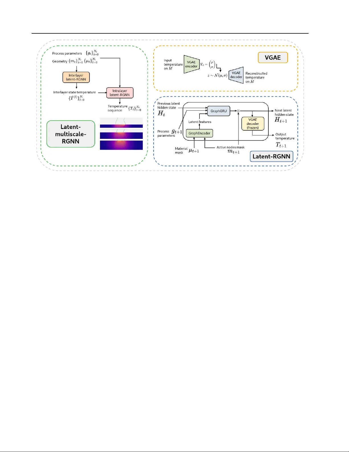
Stable Long-Horizon Spatiotemporal Prediction on Meshes Using Latent Multiscale Recurrent Graph Neural Networks Lionel Salesses, Larbi Arbaoui, T ariq Benamara, Arnaud Francois, Car oline Sain vitu Cenaero Gosselies, Belgium lionel.salesses@cenaero.be Abstract Accurate long-horizon prediction of spatiotempo- ral ﬁelds on complex geometries is a fundamental challenge in scientiﬁc machine learning, with ap- plications such as additi ve manuf acturing where temperature histories go vern defect formation and mechanical properties. High-ﬁdelity simulations are accurate but computationally costly , and de- spite recent advances, machine learning methods remain challenged by long-horizon temperature and gradient prediction. W e propose a deep learn- ing framew ork for predicting full temperature his- tories directly on meshes, conditioned on geom- etry and process parameters, while maintaining stability ov er thousands of time steps and gen- eralizing across heterogeneous geometries. The framew ork adopts a temporal multiscale architec- ture composed of two coupled models operating at complementary time scales. Both models rely on a latent recurrent graph neural network to cap- ture spatiotemporal dynamics on meshes, while a v ariational graph autoencoder provides a compact latent representation that reduces memory usage and improves training stability . Experiments on simulated po wder bed fusion data demonstrate accurate and temporally stable long-horizon pre- dictions across div erse geometries, outperform- ing existing baseline. Although ev aluated in two dimensions, the frame work is general and e xten- sible to physics-dri ven systems with multiscale dynamics and to three-dimensional geometries. K eywords Long-Horizon Prediction · Multiscale Modeling · Additiv e Manufacturing · Scientiﬁc Machine Learning · Graph Autoencoder 1. Introduction Accurate long-horizon prediction of spatiotemporal ﬁelds deﬁned on complex and ev olving geometries is a central challenge in scientiﬁc machine learning. Such problems arise across a wide range of physical systems, including additiv e manufacturing [ 1 ], climate and weather modeling [ 2 ], [ 3 ], and ﬂuid dynamics [ 4 ], where system dynamics exhibit strong coupling between fast local phenomena and slow global e volution. Learning models that are both tempo- rally stable ov er long horizons and computationally ef ﬁcient remains an open problem, particularly when predictions must be made directly on irregular meshes [ 5 ], [ 6 ]. Additi ve manufacturing provides a representati ve and practically rel- ev ant instance of this challenge. During metal po wder bed fusion, the temperature history gov erns defect formation, residual stresses, and ﬁnal mechanical properties (see [ 7 ] and [ 8 ]). While high-ﬁdelity numerical solvers can accu- rately capture these thermal dynamics, their computational cost precludes real-time inference and limits large-scale de- sign exploration (see [ 9 ] and [ 10 ]). While recent machine learning approaches hav e shown promise in accelerating thermal prediction, achie ving reliable long-range forecasts of temperature ﬁelds and gradients on v ariable geometries remains difﬁcult in practice [ 11 ]. A ke y difﬁculty stems from the intrinsic temporal multiscale structure of the un- derlying physics. In additive manufacturing, short-term intralayer dynamics are dominated by highly localized laser - material interactions, whereas long-term interlayer dynam- ics are governed by heat diffusion and cumulative energy deposition. T reating these disparate time scales within a single monolithic sequence model often leads to unstable training, excessi ve memory usage, or error accumulation ov er long horizons [ 12 ]. In this work, we propose a Latent Multiscale Recurrent Graph Neural Network (LM-RGNN) frame work that e xplicitly lev erages this temporal separation. Stable Long-Horizon Spatiotemporal Prediction on Meshes Using Latent Multiscale Recurrent Graph Neural Networks Our approach decomposes long-horizon prediction into two coupled but independently trained models operating at com- plementary time scales. Both models perform sequence prediction directly on meshes using a recurrent graph neural network, while a V ariational Graph Autoencoder (V GAE) provides a compact latent representation of temperature ﬁelds. This latent formulation substantially reduces mem- ory requirements and facilitates stable information propaga- tion ov er long temporal horizons. From a machine learning perspectiv e, our contribution is a general latent multiscale modeling strategy for long-horizon spatiotemporal predic- tion on graphs, rather than a task-speciﬁc architecture. The proposed frame work is designed to accommodate v ariable meshes, long sequences, and multiscale temporal dynamics, which are common across many physics-dri ven learning problems. Additiv e manufacturing serves as a challenging testbed that highlights these characteristics but does not constrain the applicability of the method. W e ev aluate the proposed approach on simulated po wder bed fusion data and demonstrate improv ed predicti ve accuracy , temporal stability , and computational efﬁcienc y compared to an exist- ing graph-based baseline [ 11 ]. Beyond temperature ﬁelds, the model accurately captures derived quantities such as spatial and temporal gradients and melt-pool localization. While our experiments focus on two-dimensional simula- tions, the framework naturally e xtends to three-dimensional geometries and other multiscale physical systems. Overall, this work advances the state of long-horizon spatiotempo- ral modeling on graphs by introducing a latent multiscale formulation that improv es stability and scalability , offering a general tool for scientiﬁc machine learning applications characterized by coupled fast and slow dynamics. Poten- tial extensions and application domains are discussed in Appendix A . 2. Related W ork Machine Learning for Spatiotemporal and Physics- Based Modeling. Learning long-horizon spatiotemporal dynamics gov erned by PDEs remains a central challenge in scientiﬁc machine learning. Autoregressi ve models, while widely used due to their simplicity , often suffer from error accumulation and instability over long rollouts, particularly when applied to high-dimensional physical ﬁelds. Lippe et al. [ 12 ] sho w that standard autoregressi ve models often fail to produce stable and accurate rollout predictions due to their inability to capture the high-frequency components of PDE solutions. T o address this limitation, they introduce PDE-Reﬁner , a diffusion-inspired reﬁnement framew ork that enhances high-frequency modeling for autoregressi ve predictors operating on ﬁxed re gular grids through a multi- step reﬁnement strategy . The method is validated on ﬂuid dynamics benchmarks, yielding substantial impro vements in rollout accuracy ov er horizons of up to 1000 time steps. Graph-based models have emerged as a natural paradigm for learning physics on unstructured domains. The EA- GLE framework [ 13 ] introduces an autoregressiv e graph encoder-decoder architecture combining mesh clustering with a core attention mechanism to model turbulent ﬂow dynamics directly on simulation meshes. T rained on CFD data, EA GLE demonstrates the ability to predict ﬂo ws across varying two-dimensional geometries, with ev aluation over horizons of up to 250 time steps showing a gradual, though limited, error growth. Similarly , the T emporal Graph Net- work (TGN) frame work [ 6 ] explores recurrent graph-based architectures for physics prediction on unstructured meshes, highlighting the dif ﬁculty of achieving long-horizon stabil- ity due to the joint spatialtemporal comple xity of physical systems. Recent work has also explored attention-based and operator-learning approaches for spatiotemporal model- ing. The ASNO framework [ 14 ] proposes an autoregressi ve architecture that decouples spatial and temporal modeling using attention mechanisms, follo wed by a neural opera- tor to predict spatiotemporal ﬁelds. ASNO is ev aluated on benchmark PDE systems, including melt pool prediction in additive manufacturing. Operating on ﬁxed grids, it re- ports stable rollouts up to 95 time steps with reduced error accumulation compared to baselines. Machine Learning for Additive Manufacturing and Thermal Modeling. Sev eral studies in additiv e manufac- turing employ Physics-Informed Neural Networks (PINNs) to achie ve accurate thermal predictions for a speciﬁc geome- tries [ 15 , 16 ], achie ving good melt pool reconstruction but typically focusing on limited geometries and short predic- tion horizons. T ian et al. [ 1 ] combine physics-informed RNNs with con volutional LSTMs to autoregressi vely pre- dict thermal histories on regular grids for thin-wall geome- tries, achieving an RMSE of about 20 °C over short-term horizons (11.25 s), demonstrating the potential of recurrent formulations for thermal modeling, b ut without ev aluation in long-horizon rollout settings. Graph-based learning has recently gained traction in additiv e manufacturing due to its ability to operate directly on v ariable part meshes. Choi et al. [ 11 ] propose a GNN-RNN architecture trained on addi- tiv e manufacturing simulations to predict thermal histories for unseen complex three-dimensional geometries. Operat- ing at the subsequence le vel, their model achie ves accurate and stable predictions ov er horizons of up to 50 time steps. Considering to its strong performance and close method- ological relev ance, this approach is adopted as a baseline in the present work and detailed in Appendix D . Positioning of This W ork. In contrast to prior approaches, our work targets long-horizon spatiotemporal prediction on irregular meshes by explicitly le veraging the temporal mul- tiscale structure of the underlying physics. Unlike single- scale autoregressiv e graph models such as EAGLE [ 13 ] 2 Stable Long-Horizon Spatiotemporal Prediction on Meshes Using Latent Multiscale Recurrent Graph Neural Networks or subsequence-based approaches in additive manufactur- ing [ 11 ], we decompose the prediction task into coupled interlayer and intralayer models operating at complemen- tary time scales. This design enables stable prediction ov er thousands of time steps while remaining computationally efﬁcient. Moreover , whereas diffusion-based reﬁnement strategies [ 12 ] and neural operator approaches [ 14 ] primar- ily operate on ﬁxed grids, our framew ork directly models ﬁelds on v ariable meshes using a latent recurrent graph neural network. While ev aluated in the context of addi- tiv e manufacturing, the proposed latent multiscale RGNN framew ork is general and applicable to a broad class of physics-dri ven systems characterized by coupled f ast local dynamics and slow global e volution. 3. Additive Manufacturing Benchmark and Dataset The task addressed in this work is to predict the com- plete temperature history during the additiv e manufacturing process using a deep learning approach capable of han- dling variable part geometry . The present study focused on two-dimensional geometries, which already pose signiﬁ- cant modeling challenges; ho wev er , the proposed machine learning framework is explicitly designed with scalability to three-dimensional parts in mind, where data generation costs, memory requirements, and computational complexi- ties become substantially higher . The task can be formulated around the following objecti ves: (i) Achiev e temporally stable long-horizon predictions of the full temperature ev olution deﬁned on geometry- speciﬁc simulation meshes. (ii) Accurately predict temperature ﬁelds with respect to physically and application-rele vant metrics, including spatial and temporal temperature gradients that are critical to printed part quality (see [ 17 ] or [ 18 ]). (iii) Generalize ef fectiv ely to geometries unseen during training. (iv) Control memory consumption to ensure scalability and to anticipate the signiﬁcant increase in memory foot- print of three-dimensional simulations. (v) Ensure inference times is compatible with near real- time prediction, enabling future applications such as process monitoring. The dataset is deriv ed from two-dimensional numerical sim- ulations performed using a ﬁnite element-based thermal solver . Those simulations are designed to predict spatial and temporal e volution of the temperature during additi ve manufacturing of metallic parts with a particular focus on the po wder bed fusion process. Numerical simulations are based on a layer by layer progressi ve approach that employs mesh element acti vation techniques. For each layer , the thermal ev olution is characterized by a distinct heating and cooling phase. During the heating phase, thermal responses are computed using a moving Gaussian heat source with an alternating linear laser path. Each activ ated layer is com- posed of a metallic powder re gion and a solid metal region targeted by the laser heat source. More details on the manu- facturing process and the modeling hypothesis can be found in Appendix B . The dataset is designed to train and develop a deep learning approach focusing on geometrical charac- teristics. Process parameters including laser course speed, laser power , cooling time and scan trajectory are kept ﬁxed throughout this study . Each simulation is associated with a parameterized geometry that satisﬁes additiv e manufactura- bility constraints, as detailed in Appendix B.1 . An example of such a geometry is sho wn in Figure 1 . Additional de- tails on the dataset generation and the underlying simulation model are provided in Appendix B.2 and Appendix B.3 , respectiv ely . F igure 1. Example of printed geometry . Metallic po wder is in gray , the ﬁnal printed part is in blue and the part boundaries are highlighted in green. For each simulation in the dataset, we have access to the computational mesh, including its topology , node coordi- nates, and material mask, as well as the laser process param- eters, namely the time-resolved laser position and power . The simulated temperature ﬁeld is provided at each simu- lation time step for all currently unmasked nodes. Since the simulation domain increases progressively in a layer-by- layer manner during the printing process, an acti ve-node mask is av ailable at every time step. T emperature ﬁelds are deﬁned at mesh nodes and recorded for each simulation time step (see Figure 2 for representativ e snapshots). The length of the resulting temperature sequences depends on the part geometry and, in the present dataset, ranges from 6600 to 12000 time steps (corresponding to approximately 1600s to 3000s). T emperature values span from a minimum of 20°C to a maximum of approximately 2100°C. The highest temperatures occur in the vicinity of the laser beam, where metallic po wder melts do wn to form the melt pool. This region is characterized by steep temperature gradients and complex physical processes, including phase change, which are modeled through the inclusion of a latent heat term in the gov erning equations. The 140 generated simulations are 3 Stable Long-Horizon Spatiotemporal Prediction on Meshes Using Latent Multiscale Recurrent Graph Neural Networks randomly partitioned into 80 simulations for training, 20 for validation, and 40 for testing. F igure 2. T emperature ﬁeld snapshots for a ﬁxed printed geometry at multiple time steps. The green lines indicate the part boundaries, enclosing the solid metallic region. The temperature is simulated for both metallic part and the surrounding powder . 4. Latent Multiscale Recurrent Graph Architectur e In this section, we introduce an architecture for predicting the temperature history of a printed part from process param- eters and geometric information. The proposed approach adopts a time-multiscale modeling strategy based on two coupled models, each operating at a distinct temporal scale. Both models are built upon two core components: a RGNN, which enables the sequential modeling of temperature ﬁelds deﬁned on a mesh, and a VGAE, which provides a compact latent representation of the temperature ﬁelds. 4.1. Architectur e Design Motivations Since the temperature ﬁelds are deﬁned on simulation meshes, it is natural and advantageous to operate directly on mesh-based data using GNNs, thereby av oiding interpo- lation onto a ﬁxed snapshot grid, which would introduce additional approximation errors. In particular, mesh repre- sentations more accurately capture part interfaces, whereas image-based interpolations tend to blur these interfaces, leading to aliasing and loss of geometric ﬁdelity . GNNs enable the processing of both local mesh connecti vity and global structural features, allo wing them to simultaneously model ﬁne-scale details and the overall geometry of the part. As a result, GNNs are well suited to this class of problems. The objecti ve of this work is to learn a mapping from the process parameters (speciﬁcally the laser path) to time-resolved sequences of temperature ﬁelds ov er very long temporal horizons. This requirement necessitates a model with strong temporal stability and minimal error ac- cumulation. As discussed in Appendix C.1 , RNN are well suited to this class of problems; howe ver , this approach poses signiﬁcant computational challenges. In particular, the memory footprint required for backpropagation through long sequences becomes prohibitiv e. T o address this limita- tion, we adopt T runcated Backpropagation Through T ime (TBPTT) [ 19 ], which restricts backpropagation to a limited number of time steps while allo wing the forward pass to proceed sequentially . This strategy substantially reduces memory usage while maintaining the ability to model long- term temporal dependencies. A second major challenge arises from the v anishing and exploding gradient phenom- ena commonly encountered in recurrent neural networks. T o mitigate these effects, we employ an interlayer and in- tralayer splitting strategy (detailed belo w), which allows the RNN to be trained on coarser temporal sequences. This strat- egy enables the interlayer and intralayer models to be trained independently , facilitating modular de velopment and more effecti ve prototyping. T o extend recurrent neural networks to graph-structured data, we introduce a RGNN architecture that combines a standard recurrent unit (speciﬁcally a Gated Recurrent Unit (GR U)) with graph neural network layers. For computational ef ﬁciency , the RGNN operates on a low- dimensional latent representation of the temperature ﬁelds rather than the full high-dimensional state, substantially reducing memory usage and alleviating GPU constraints on batch size and TBPTT sequence length. The tempera- ture ﬁelds deﬁned on complex geometries e xhibit multiple sources of v ariability , including global geometric structure and highly localized thermal dynamics associated with the laser-induced melt pool. T o obtain such latent representa- tions, we employ a V GAE, which generalizes the classical V AE to graph-structured data (see [ 20 ] and [ 21 ]). The use of hierarchical graph pooling and unpooling operations allows the VGAE to e xtract multiscale features from both the part geometry and the temperature ﬁeld, making it well suited for downstr eam recurrent modeling. W e now provide a detailed description of the components that constitute the proposed architecture. 4.2. GraphGR U: Graph Gated Recurrent Unit The standard formulation of the GRU operates on vector- valued inputs and hidden states. This formulation has been extended to structured data such as images and graphs by replacing linear transformations with conv olutional or graph- based operators [ 22 ]. In this work, we generalize the GR U to graph-structured data by replacing the matrix multipli- cations in the classical GR U with Message-Passing Graph 4 Stable Long-Horizon Spatiotemporal Prediction on Meshes Using Latent Multiscale Recurrent Graph Neural Networks Neural Netw orks (MPGNNs). Implementation details of the resulting GraphGR U module are provided in Appendix C.2 . 4.3. RGNN: Recurrent Graph Neural Netw ork Let T 0 denote the initial temperature and M the part mesh, which is represented as a graph ( A, E ) , where A is the adjacency matrix and E contains edge features encoding geometric information such as edge lengths and unit direc- tion vectors. The initial hidden state H 0 is constructed by normalizing the initial temperature ﬁeld and padding it with zeros to match the recurrent hidden state size. At each time step t , the model is provided with an activ e-node mask m t , a material mask µ t indicating the local material state (metal or powder), and a v ector of global attributes g t +1 that encodes process parameters, including changes in laser position and power since the previous time step. The RGNN ev olves according to the following recurrent update (see Figure 11 ): X t +1 = m t +1 ⊕ µ t +1 , H t +1 = GraphGR U( X t +1 , H t , g t +1 ) ⊙ m t +1 , T t +1 = H t +1 [0] , (1) where the hidden state H t is a node-feature tensor whose ﬁrst component corresponds to the nodal temperature T t . 4.4. V GAE: V ariational Graph A uto-Encoder The VGAE takes as input a temperature ﬁeld T true deﬁned on a mesh, represented as a graph ( A, E ) , together with a mask of active nodes m . Its purpose is to encode the tem- perature ﬁeld into a compact latent representation deﬁned on a reduced, latent graph. The learned latent representa- tion enables downstream models to operate directly in latent space, substantially reducing memory consumption. Im- plementation details of the V GAE module are provided in Appendix C.4 . 4.5. Latent-RGNN The RGNN introduced in Section 4.3 can be extended to operate directly in latent space. The recurrent hidden state may be initialized either to zero or by encoding the initial temperature ﬁeld using a pre-trained VGAE encoder . In the latter case, the initial latent state is set to the node-wise mean of the latent distrib ution predicted by the encoder . The latent-RGNN produces a sequence of latent representations, which are subsequently decoded into temperature ﬁelds us- ing the pre-trained VGAE decoder with ﬁxed parameters. The primary motiv ation for the latent-RGNN design is to reduce GPU memory consumption and av oid computation- ally expensi ve operations on high-dimensional ﬁelds. More details are giv en is Appendix C.5 . 4.6. Time-Multiscale Strategy The layer-by-layer nature of the additi ve manufacturing pro- cess naturally induces two distinct temporal scales: (i) an interlayer scale, corresponding to the temperature ﬁeld at the completion of each printed layer , and (ii) an intralayer scale, corresponding to the ﬁne-grained temporal ev olution of the temperature ﬁeld during the printing of a single layer . W e exploit this structure by introducing a time-multiscale modeling strategy based on two coupled b ut independently trained models, as summarized in Figure 3 . The interlayer model is trained to predict the temperature ﬁeld at the end of each layer and capture long-term thermal dynamics dom- inated by heat diffusion and cumulati ve heat accumulation effects. Conditioned on these interlayer predictions, the intralayer model is trained to reconstruct the temperature ev olution within each layer . Speciﬁcally , it takes as input the predicted initial temperature at the start of a layer , along with the layer associated process parameters, and outputs the transient temperature ﬁelds until layer completion. The intralayer model focuses on short-term dynamics associ- ated with laser motion and melt-pool phenomena, which are characterized by large but spatially localized temperature gradients. Both models are trained on substantially shorter temporal sequences than a full-sequence RGNN, resulting in improved training stability and reduced probability of vanishing and exploding gradient ef fects. In addition, this two-stage design enables more ef ﬁcient inference: once the interlayer predictions are obtained, intralayer temperature ev olution for all layers can be computed in parallel. This contrasts with full-sequence RGNNs, which require strictly sequential prediction across all time steps and thus incur signiﬁcantly higher inference costs. Let { T t } N t =0 denote the sequence of temperature ﬁelds o ver time. This sequence can be partitioned according to the layer structure of the pro- cess into a collection of layer-wise subsequences { T ( l ) } L l =0 , where L denotes the total number of layers. Each subse- quence T ( l ) = { T t } N l t =0 , corresponds to the temperature ev olution during the printing of layer l , with N l denoting the number of time steps associated with that layer . W e further denote ˜ T ( l ) the temperature ﬁeld after completion of printing layer l . Interlayer Model. The interlayer model, implemented us- ing the latent-RGNN architecture, is trained to predict the se- quence of layer-wise terminal temperature ﬁelds { ˜ T ( l ) } N l l =0 . It takes as input global geometric information, including acti ve-node masks and material masks, as well as a sequence of layer-le vel process descriptors such as layer width, print- ing duration, and cooling duration. Intralayer Model. The intralayer model, also based on the latent-RGNN architecture, is trained to predict the within-layer temperature ev olution T ( l ) for each layer l . 5 Stable Long-Horizon Spatiotemporal Prediction on Meshes Using Latent Multiscale Recurrent Graph Neural Networks F igure 3. Overvie w of the LM-RGNN architecture and its main components, including the latent-RGNN and the VGAE. It is conditioned on the initial temperature ﬁeld at the start of the layer , as predicted by the interlayer model, together with the same global geometric information and a sequence of time-resolved process parameters. Latent-Multiscale-RGNN (LM-RGNN). The LM- RGNN refers to the coupled architecture obtained by integrating the interlayer and intralayer models described abov e (see Figure 3 ). 5. Experiments and Results All details regarding the optimizer , learning rate scheduler , temperature sequence subsampling strategy , and training hyperparameters are provided in Appendix E . 5.1. Evaluation Metrics W e assess model performance using a comprehensi ve set of metrics, including Mean Absolute Error (MAE), Mean Absolute Percentage Error (MAPE), Mean Maximum Error (MME), melt-pool Intersection over Union (mpIoU), and temporal MAE (t-MAE). In addition, we e valuate errors on spatial and temporal temperature gradients through the MAE of spatial gradients ( MAE ∇ xy ) and temporal gradients ( MAE ∇ t ). The t-MAE metric is used to quantify temporal stability of the predictions. In addition to predictiv e accu- racy , we report the number of model parameters, memory consumption at training-time, and per -time-step inference time measured in milliseconds. Further details on the e val- uation metrics and experimental protocol are provided in Appendix F . 5.2. Baseline As a baseline for comparison, we reimplemented the Decoupled-RGNN architecture proposed by [ 11 ]. This model is designed to predict the temperature evolution throughout the printing process and to generalize across previously unseen geometries. Additional details regarding the architecture and our implementation are provided in Appendix D . 5.3. V GAE Model Perf ormance The VGAE model performances are reported in Appendix G.2 . For all latent-based models considered in the follo wing, we employ a VGAE trained with a latent dimensionality of 16, which produced the best predictiv e accuracy . Overall, the VGAE e xhibits fav orable performance with respect to the considered objectiv es, yielding low reconstruction error , stable behavior o ver time, satisfactory accurate predictions of melt pool extent, and controlled worst-case errors. 5.4. LM-RGNN Model Perf ormance T emperature Prediction Accuracy . T ables 1 and 2 re- port the performance metrics of the interlayer , intralayer , and LM-RGNN models, together with their ablated variants and the Decoupled-RGNN baseline. A detailed analysis of the differences between each model and its ablated coun- terpart is pro vided in Section 5.5 . Figures 16 and 17 in Appendix G.3 provide a visual comparison of temperature predictions, for a representati ve geometry and time step, between the LM-RGNN model and the Decoupled-RGNN 6 Stable Long-Horizon Spatiotemporal Prediction on Meshes Using Latent Multiscale Recurrent Graph Neural Networks baseline. Overall, the LM-RGNN (which combines the pre- dictions of the interlayer and intralayer models) achiev es consistently better performance than the Decoupled-RGNN baseline. Improv ements are observed across temperature prediction accuracy , spatial and temporal gradient errors, and melt-pool estimation. These gains are obtained with a memory footprint comparable to the baseline, while in- ference time is only marginally higher (+0.97ms/time step). The interlayer and intralayer models exhibit similar MAE values; howe ver , their MAPE scores differ substantially . This difference is primarily due to the lo wer temperature magnitudes observed in interlayer data, which correspond to end-of-layer cooling phases, as opposed to intralayer se- quences that include acti ve laser heating and substantially higher temperatures. As a result, relativ e errors are mag- niﬁed for the interlayer model. In contrast, the interlayer model attains lo wer MME values, reﬂecting the absence of extreme temperature peaks during cooling periods. W e further note that the VGAE was trained on the full set of tem- perature ﬁelds rather than being specialized for interlayer states, which represent only a small fraction of the dataset. T raining a dedicated VGAE on interlayer temperature ﬁelds could therefore further improv e interlayer prediction accu- racy . Finally , although the interlayer model e xhibits a higher per-step inference time than the intralayer model due to its larger number of parameters, this has a limited impact on the overall inference cost of the LM-RGNN. Indeed, the interlayer model is in voked only once per printed layer (100 time steps in total), whereas the intralayer model accounts for the majority of time-step predictions. T emporal Stability . Figure 6 reports the t-MAE for the LM-RGNN and the Decoupled-RGNN baseline. The LM- RGNN exhibits strong temporal stability , characterized by low-amplitude oscillations and no noticeable error accumu- lation o ver time. In contrast, the Decoupled-RGNN baseline shows a gradual b ut persistent increase in error , together with more pronounced temporal ﬂuctuations. Further in- sight is provided in Figures 4 and 5 , which demonstrate the temporal stability of the interlayer and intralayer models, respectiv ely . For the intralayer setting, larger error oscil- lations are observed at late time steps. This behavior can be partially e xplained by data sparsity , which affects the reliability of the a veraged error estimates, as only a lim- ited number of simulations extend beyond approximately 2800s. Consistent with the beha vior observed for the VGAE in Figure 15 , an initial error peak is present at early time steps. This effect arises from the computation of MAE ov er a temporally v arying activ e domain and reﬂects error con- centration during the early stages of the printing process. A detailed analysis of this phenomenon is provided in the Appendix G.1 . F igure 4. T emporal MAE (t-MAE) on the test set for the interlayer model, compared with its full-dimensional (non-latent) counter- part. F igure 5. T emporal MAE (t-MAE) on the test set for the intralayer model, compared with its ablated variants. F igure 6. T emporal MAE on the test set for the LM-RGNN model, compared with its ablated variant and the Decoupled-RGNN base- line. 5.5. Ablation Study T ables 1 and 2 , together with Figures 4 , 5 , and 6 , report performance metrics and temporal MAE results for the in- terlayer , intralayer, and LM-RGNN models, as well as their corresponding ablated variants. For the interlayer setting, we compare the latent-RGNN architecture with a non-latent ablation that operates directly on full-resolution temperature ﬁelds while maintaining a comparable model size. The non- latent variant e xhibits substantially higher training variabil- ity , increased memory consumption, and degraded perfor- 7 Stable Long-Horizon Spatiotemporal Prediction on Meshes Using Latent Multiscale Recurrent Graph Neural Networks T able 1. Comparison of performance metrics on the test set across the proposed models, their ablated variants (marked by the , → symbol) , and the baseline. Model MAE (°C) MAPE (%) MME (°C) mpIoU MAE ∇ xy (°C/mm) MAE ∇ t (°C/s) Parameters Interlayer 7.29 ± 0.17 4.48 ± 0.22 44.5 ± 0.5 2.10 ± 0.05 0.76 ± 0.09 85k  → w/o latent 17.80 ± 9.16 4.73 ± 1.57 95.0 ± 40.6 4.65 ± 1.54 0.40 ± 0.18 91k Intralayer 6.48 ± 0.19 2.20 ± 0.010 108.7 ± 2.80 0.87 ± 0.0016 2.46 ± 0.030 1.61 ± 0.020 42k  → w/o latent 6.80 ± 0.34 2.43 ± 0.18 50.6 ± 2.0 0.91 ± 0.0081 2.27 ± 0.10 1.28 ± 0.064 41k LM-RGNN 6.50 ± 0.10 2.58 ± 0.002 108.7 ± 0.28 0.85 ± 0.0017 2.44 ± 0.030 1.98 ± 0.0031 127k  → w/o latent & multiscale strategy 26.28 ± 1.45 7.25 ± 1.12 111.46 ± 5.1 0.69 ± 0.097 5.98 ± 1.30 7.13 ± 0.84 131k Baseline Decoupled-RGNN 26.57 ± 3.44 6.59 ± 1.26 170.9 ± 19.5 0.67 ± 0.032 6.41 ± 1.28 7.79 ± 0.70 111k T able 2. Comparison of per-time-step inference time and training- time memory pressure across the proposed models, their ablated variants (mark ed by the , → symbol), and the baseline. Model Inference time (ms) Mem. pressure Interlayer 30.4 Low  → w/o latent 30.9 Medium Intralayer 12.35 Low  → w/o latent 14.28 Medium LM-RGNN 14.47 Low  → w/o latent & multiscale strategy 68.19 High Baseline Decoupled-RGNN 13.50 Low mance across most metrics, with the e xception of MAE ∇ t , which remains low for both v ariants. In the intralayer setting, the latent-RGNN and its non-latent counterpart achieve com- parable performance. The non-latent model yields slightly improv ed MME, melt-pool estimation, and gradient-related metrics; howe ver , these gains come at the cost of higher inference time and signiﬁcantly increased memory usage due to full-ﬁeld processing. Consequently , for the intralayer model, operating in the latent space primarily provides ben- eﬁts in terms of memory efﬁcienc y rather than predicti ve accuracy . Overall, latent representations yield more pro- nounced performance gains for the interlayer model than for the intralayer model. W e assume that this dif ference arises from the nature of the temporal dynamics: consecu- ti ve intralayer states are highly similar, with changes largely conﬁned to local regions around the laser path, whereas in- terlayer states dif fer more substantially due to layer addition, extended thermal dif fusion, and cumulativ e energy input. In this context, predicting intralayer transitions is well suited to message-passing architectures with limited receptiv e ﬁelds. By contrast, the latent representation, deﬁned on a coarser mesh, enables more ef ﬁcient global information propag ation for interlayer dynamics, followed by accurate reconstruction via the pretrained VGAE decoder . Finally , we compare the LM-RGNN with an ablated non-latent RGNN trained on full sequences without temporal multiscale decomposition. The ablated model performs signiﬁcantly worse. One contrib ut- ing factor is the dif ﬁculty of training RGNNs on extremely long sequences (up to 1800 time steps after subsampling), which leads to poor gradient propagation, unstable optimiza- tion, and oscillatory training loss. In addition, operating on full-resolution temperature ﬁelds substantially increases memory requirements, forcing the use of very small batch sizes and further degrading training stability . 6. Conclusion Contributions. W e introduced a LM-RGNN frame work for predicting full temperature histories in additi ve manufac- turing directly on the part mesh, conditioned on geometric and process parameters. The integration of a VGAE with a temporal multiscale RGNN enables stable and accurate long- horizon prediction while mitigating the memory burden as- sociated with high-resolution simulation data. The explicit decomposition into interlayer and intralayer models allows the framework to capture both slow , diff usion-dominated thermal ev olution and fast, laser -induced spatially local- ized dynamics, leading to impro ved accurac y of predicted temperature ﬁelds, spatial and temporal gradients, and melt- pool localization relativ e to existing baseline. Extensiv e experiments on simulated powder bed fusion data demon- strate that the proposed architecture achie ves accurate and temporally stable predictions o ver thousands of time steps across div erse geometries. Limitations and Future W ork. While the proposed framew ork is designed with three-dimensional geometries and broader process generalization in mind, the present study is limited to two-dimensional simulations and a single powder bed fusion process with ﬁxed parameters. More- ov er , the models are trained exclusiv ely on simulated data, and further in vestigation is needed to assess robustness to process variability and transferability to e xperimental mea- surements. Broader Impact. Beyond additive manufacturing, the pro- posed latent-multiscale-RGNN frame work pro vides a gen- eral approach for modeling physics-driv en systems with coupled fast and slow temporal dynamics on complex ge- ometries. Potential application domains include ﬂuid dy- namics and climate and weather modeling (see Appendix A for a detailed discussion). 8 Stable Long-Horizon Spatiotemporal Prediction on Meshes Using Latent Multiscale Recurrent Graph Neural Networks Impact Statement This paper presents work whose goal is to advance the ﬁeld of Machine Learning. There are many potential societal consequences of our work, none which we feel must be speciﬁcally highlighted here. Acknowledgments This work is supported by the “ ARIA C by DigitalW allo- nia4.ai” reasearch project (grant agreement No 2010235 – TRAIL institute) and beneﬁted from computational re- sources made available on Lucia, the Tier -1 supercom- puter of the W alloon Region, infrastructure funded by the W alloon Region (grant agreement No 1910247). This work is supported by the European Regional De velopment Fund (ERDF/FEDER) and the W alloon Region of Belgium through project 364 Cenaero_AdviseAM (programme 2021- 2027). References [1] Mingxuan T ian, Haochen Mu, T ao Liu, Mengjiao Li, Donghong Ding, and Jianping Zhao. Physics-informed machine learning-based real-time long-horizon tem- perature ﬁelds prediction in metallic additiv e manu- facturing. Communications Engineering , 4(1):168, 2025. [2] Y ogesh V erma, Markus Heinonen, and V ikas Garg. Climode: Climate and weather forecasting with physics-informed neural odes. arXiv pr eprint arXiv:2404.10024 , 2024. [3] Ilan Price, Alvaro Sanchez-Gonzalez, Ferran Alet, T om R Andersson, Andrew El-Kadi, Dominic Masters, T imo Ewalds, Jacklynn Stott, Shakir Mohamed, Peter Battaglia, et al. Probabilistic weather forecasting with machine learning. Natur e , 637(8044):84–90, 2025. [4] Rui Gao, Shayan Heydari, and Rajee v K Jaiman. T o- wards spatio-temporal prediction of cavitating ﬂuid ﬂow with graph neural networks. International J our- nal of Multiphase Flow , 177:104858, 2024. [5] Ling Zhao, Y ujiao Song, Chao Zhang, Y u Liu, Pu W ang, T ao Lin, Min Deng, and Haifeng Li. T - GCN: A temporal graph con volutional network for trafﬁc prediction. IEEE transactions on intelligent transportation systems , 21(9):3848–3858, 2019. [6] Miaocong Y ue, Huayong Liu, Xinghua Chang, Laip- ing Zhang, and T ianyu Li. TGN: A temporal graph network for physics prediction. Applied Sciences , 14(2):863, 2024. [7] Shubhav ardhan Ramadurga Narasimharaju, W enhan Zeng, T ian Long See, Zicheng Zhu, Paul Scott, Xi- angqian Jiang, and Shan Lou. A comprehensi ve revie w on laser po wder bed fusion of steels: Processing, mi- crostructure, defects and control methods, mechanical properties, current challenges and future trends. Jour- nal of Manufacturing Pr ocesses , 75:375–414, 2022. [8] Peiying Bian, Ali Jammal, Ke wei Xu, F angxia Y e, Nan Zhao, and Y un Song. A re view of the e volu- tion of residual stresses in additi ve manufacturing during selecti ve laser melting technology . Materials , 18(8):1707, 2025. [9] Michele Chiumenti, Eric Nei va, Emilio Salsi, Miguel Cervera, Santiago Badia, Joan Moya, Zhuoer Chen, Caroline Lee, and Christopher Davies. Numerical mod- elling and experimental validation in selective laser melting. Additive Manufacturing , 18:171–185, 2017. [10] Christian Burkhardt, Paul Steinmann, and Julia Mergheim. Thermo-mechanical simulations of pow- der bed fusion processes: accuracy and efﬁcienc y . Ad- vanced Modeling and Simulation in Engineering Sci- ences , 9(1):18, 2022. [11] Jin Y oung Choi, Sina Malakpour Estalaki, Daniel Quispe, Rujing Zha, Ro wan Rolark, Mojtaba Mozaf- far , and Jian Cao. T ransfer learning enabled geometry , process, and material agnostic RGNN for tempera- ture prediction in directed energy deposition. Additive Manufacturing , page 104876, 2025. [12] Phillip Lippe, Bas V eeling, Paris Perdikaris, Richard T urner, and Johannes Brandstetter . Pde-reﬁner: Achieving accurate long rollouts with neural pde solvers. Advances in Neural Information Pr ocessing Systems , 36:67398–67433, 2023. [13] Steev en Janny , Aurélien Beneteau, Madiha Nadri, Julie Digne, Nicolas Thome, and Christian W olf. Eagle: Lar ge-scale learning of turbulent ﬂuid dy- namics with mesh transformers. arXiv preprint arXiv:2302.10803 , 2023. [14] V ispi Nevile Karkaria, Doksoo Lee, Y i-Ping Chen, Y ue Y u, and W ei Chen. ASNO: An interpretable attention-based spatio-temporal neural operator for robust scientiﬁc machine learning. In ICML 2025 W orkshop on Reliable and Responsible F oundation Models , 2025. [15] Qiming Zhu, Zeliang Liu, and Jinhui Y an. Machine learning for metal additi ve manufacturing: predict- ing temperature and melt pool ﬂuid dynamics using physics-informed neural networks. Computational Mechanics , 67(2):619–635, 2021. 9 Stable Long-Horizon Spatiotemporal Prediction on Meshes Using Latent Multiscale Recurrent Graph Neural Networks [16] Shuheng Liao, Tianju Xue, Jihoon Jeong, Samantha W ebster , K ornel Ehmann, and Jian Cao. Hybrid ther - mal modeling of additive manufacturing processes using physics-informed neural networks for tempera- ture prediction and parameter identiﬁcation. Computa- tional Mechanics , 72(3):499–512, 2023. [17] Haider Ali, Hassan Ghadbeigi, and Kamran Mumtaz. Residual stress dev elopment in selective laser -melted Ti6Al4V: a parametric thermal modelling approach. The International J ournal of Advanced Manufacturing T echnology , 97(5):2621–2633, 2018. [18] Daniyal Abolhasani, SM Hossein Seyedkashi, Namhyun Kang, Y ang Jin Kim, Y oung Y un W oo, and Y oung Hoon Moon. Analysis of melt-pool behaviors during selective laser melting of AISI 304 stainless- steel composites. Metals , 9(8):876, 2019. [19] Herbert Jae ger . T utorial on training r ecurr ent neu- ral networks, covering BPPT, RTRL, EKF and the echo state network appr oach , volume 5. GMD- Forschungszentrum Informationstechnik Bonn, 2002. [20] Thomas N Kipf and Max W elling. V ariational graph auto-encoders. arXiv pr eprint arXiv:1611.07308 , 2016. [21] Mario Lino V alencia, T obias Pfaff, and Nils Thuerey . Learning distributions of complex ﬂuid simulations with diffusion graph netw orks. In The Thirteenth In- ternational Confer ence on Learning Representations , 2025. [22] Y oungjoo Seo, Michaël Def ferrard, Pierre V an- derghe ynst, and Xavier Bresson. Structured sequence modeling with graph con volutional recurrent netw orks. In International confer ence on neural information pr o- cessing , pages 362–373. Springer , 2018. [23] Alessandro Candrev a, Giuseppe De Nisco, Maur- izio Lodi Rizzini, Fabrizio D’Ascenzo, Gaetano Maria De Ferrari, Die go Gallo, Umberto Morbiducci, and Claudio Chiastra. Current and future applica- tions of computational ﬂuid dynamics in coronary artery disease. Revie ws in Cardio vascular Medicine , 23(11):377, 2022. [24] Evangelos Boutsianis, Hitendu Da ve, Thomas Frauen- felder , Dimos Poulikakos, Simon W ildermuth, Marko T urina, Y iannis V entikos, and Gregor Zund. Com- putational simulation of intracoronary ﬂo w based on real coronary geometry . European journal of Car dio- thoracic Sur gery , 26(2):248–256, 2004. [25] Cyrus T anade, Nusrat Sadia Khan, Emily Rakestra w , W illiam D Ladd, Erik W Draeger , and Amanda Ran- dles. Establishing the longitudinal hemodynamic map- ping frame work for wearable-dri ven coronary digital twins. NPJ Digital Medicine , 7(1):236, 2024. [26] Krzysztof Psiuk-Maksymo wicz, Damian Borys, Bart- lomiej Melka, Maria Gracka, W ojciech P Adamczyk, Marek Rojczyk, Jaroslaw W asilewski, Jan Głowacki, Mariusz Kruk, Marcin No wak, et al. Methodology of generation of CFD meshes and 4D shape reconstruc- tion of coronary arteries from patient-speciﬁc dynamic CT. Scientiﬁc Reports , 14(1):2201, 2024. [27] Julian Suk, Guido Nannini, Patryk Rygiel, Christoph Brune, Gianluca Pontone, Alberto Redaelli, and Jelmer M W olterink. Deep vectorised operators for pulsatile hemodynamics estimation in coronary arter- ies from a steady-state prior . Computer methods and pr ograms in biomedicine , page 108958, 2025. [28] Ziyu Ni, Linda W ei, Lijian Xu, Qing Xia, Hong- sheng Li, Shaoting Zhang, and Dimitris Metaxas. V oxel2hemodynamics: An end-to-end deep learning method for predicting coronary artery hemodynam- ics. In International W orkshop on Statistical Atlases and Computational Models of the Heart , pages 15–24. Springer , 2023. [29] Julian Suk, Pim de Haan, Phillip Lippe, Christoph Brune, and Jelmer M W olterink. Mesh neural networks for SE (3)-equiv ariant hemodynamics estimation on the artery wall. Computers in biology and medicine , 173:108328, 2024. [30] Catherine O de Burgh-Day and T ennessee Leeuwen- bur g. Machine learning for numerical weather and climate modelling: a revie w . Geoscientiﬁc Model De- velopment , 16(22):6433–6477, 2023. [31] Remi Lam, Alvaro Sanchez-Gonzalez, Matthe w Will- son, Peter W irnsberger , Meire Fortunato, Ferran Alet, Suman Ravuri, T imo Ewalds, Zach Eaton-Rosen, W ei- hua Hu, et al. Learning skillful medium-range global weather forecasting. Science , 382(6677):1416–1421, 2023. [32] T ung Nguyen, Johannes Brandstetter, Ashish Kapoor , Jayesh K Gupta, and Aditya Grov er . Climax: A foun- dation model for weather and climate. arXiv pr eprint arXiv:2301.10343 , 2023. [33] D Graham Holmes, Branden J Moore, and Stu- art D Connell. Unsteady vs. steady turbomachinery ﬂow analysis: exploiting lar ge-scale computations to deepen our understanding of turbomachinery ﬂows. In SciD A C Confer ence , 2011. 10 Stable Long-Horizon Spatiotemporal Prediction on Meshes Using Latent Multiscale Recurrent Graph Neural Networks [34] Y uki Saka, Max Gunzburger , and John Burkardt. La- tinized, improv ed LHS, and CVT point sets in hyper - cubes. International J ournal of Numerical Analysis and Modeling , 4(3-4):729–743, 2007. [35] Shaked Brody , Uri Alon, and Eran Y ahav . How at- tentiv e are graph attention networks? arXiv preprint arXiv:2105.14491 , 2021. [36] Irina Higgins, Loic Matthey , Arka P al, Christopher Burgess, Xa vier Glorot, Matthew Botvinick, Shakir Mohamed, and Alexander Lerchner . beta-v ae: Learn- ing basic visual concepts with a constrained v ariational framew ork. In International confer ence on learning r epresentations , 2017. [37] Guohao Li, Matthias Muller , Ali Thabet, and Bernard Ghanem. DeepGCNs: Can GCNs go as deep as CNNs? In Proceedings of the IEEE/CVF interna- tional confer ence on computer vision , pages 9267– 9276, 2019. [38] Nikhil Vyas, Depen Morwani, Rosie Zhao, Mujin Kwun, Itai Shapira, David Brandfonbrener , Lucas Janson, and Sham Kakade. Soap: Improving and stabilizing shampoo using adam. arXiv preprint arXiv:2409.11321 , 2024. [39] Ilya Loshchilov and Frank Hutter . Sgdr: Stochastic gradient descent with warm restarts. arXiv pr eprint arXiv:1608.03983 , 2016. 11 Stable Long-Horizon Spatiotemporal Prediction on Meshes Using Latent Multiscale Recurrent Graph Neural Networks A. General A pplicability of the Proposed Framew ork The proposed LM-RGNN frame work targets applications in volving spatiotemporal physical ﬁelds deﬁned on meshes- (potentially at high spatial resolution to capture localized phenomena) that exhibit pronounced temporal multiscale behavior arising either from the underlying physics or from time-varying inputs such as boundary conditions or external sources. The framew ork naturally accommodates v ariable geometries with geometry-speciﬁc meshes and, through masking, supports progressi vely acti vated spatial domains ov er time. Representative application domains for which the LM-RGNN architecture could be considered include, but are not limited to: • Hemodynamic ﬂo w modeling in coronary arteries with variable geometries, such as in the presence of lesions, is characterized by pronounced temporal multiscale behavior driv en by the cardiac cycle [ 23 ]. W ithin each heartbeat, fast pulsatile dynamics (systolic and diastolic pressure/ﬂo w waves) dri ve rapid changes in velocity , pressure, and wall shear stress. These ﬂuctuations occur on the order of fractions of a second and are crucial to hemodynamic function and pathology (e.g., atherogenesis) [ 24 ]. Over longer periods, v ariations across cardiac cycles (e.g., changes in heart rate, vessel compliance, stenosis se verity) modulate amplitude and phase relationships of ﬂo w features and hav e been in vestigated as potential slow temporal biomarkers [ 25 ]. The temporal multiscale structure of coronary hemodynamics makes this domain a natural candidate for multiscale sequence modeling. The LM-RGNN frame work is well aligned with this setting, as its architecture e xplicitly separates fast local dynamics from slo wer global ev olution, which may help improv e the stability and accuracy of long-horizon predictions without assuming strict periodicity . High-ﬁdelity CFD simulations on patient-speciﬁc coronary geometries are an important tool for personalized hemody- namic analysis and clinical decision support [ 26 ]. Ho we ver , these simulations are computationally intensive and dif ﬁcult to run in real time or o ver long sequences of cardiac cycles. Learning-based surrogate models that generalize across geometries and operate directly on unstructured meshes offer a promising alternati ve. In this context, the LM-RGNN frame work could be used to model ﬂo w ev olution directly on patient-speciﬁc artery meshes while maintaining temporal consistency o ver e xtended sequences. Se veral machine learning approaches have recently been e xplored for coronary hemodynamic prediction, including deep vectorized operators [ 27 ], vox el-based methods such as V oxel2Hemodynamics [ 28 ], and mesh neural networks [ 29 ]. These works demonstrate the feasibility of data-driv en hemodynamic modeling and further motiv ate the exploration of temporally multiscale, mesh-based recurrent framew orks. • W eather and climate modeling on unstructured meshes in volv es the simulation of physical ﬁelds such as temperature, pressure, wind, and humidity that ev olve across multiple temporal scales. Fast processes, including diurnal cycles, con vection, and frontal systems, typically unfold over hours to days, whereas slower phenomena such as seasonal variabilit y , interannual modes, and long-term climate trends ev olve over months to decades. This pronounced temporal multiscale structure presents a challenge for long-horizon prediction and requires modeling approaches that can simultaneously represent short-term v ariability and longer-term e volution [ 30 ]. By separating the temporal modeling into f ast and slow components, LM-RGNN can model rapid weather dynamics and slo wer climate trends in a manner similar to ho w its interlayer/intralayer decomposition isolates fast and slo w thermal phenomena in additiv e manufacturing. Contemporary numerical weather and climate models increasingly rely on v ariable-resolution or unstructured meshes to adapt spatial resolution to regions of interest, such as storms or complex topography , while maintaining computational ef ﬁciency else where [ 30 ]. Graph-based learning approaches can operate directly on such meshes, av oiding interpolation to regular grids and helping preserv e geometric ﬁdelity o ver long forecasts. In this context, the LM-RGNN architecture, which operates nati vely on simulation meshes and le verages a v ariational graph autoencoder to learn compact latent representations on coarser graphs, offers a potentially efﬁcient means of modeling spatiotemporal dynamics while controlling computational cost. Recent advances in machine learning for weather and climate forecasting further highlight the importance of ﬂexible spatial representations and long-range temporal modeling, as illustrated by approaches such as GraphCast [ 31 ] and ClimaX [ 32 ]. • Unsteady ﬂow in turbomachinery compressors results from interactions between rotating and stationary components, such as blade rows, leading to periodic ﬂuctuations in pressure, velocity , and turbulence intensity . Steady-ﬂow assumptions commonly adopted in compressor design may be insuf ﬁcient to capture these effects, particularly in the presence of rotor–stator interactions, shock dynamics, or stall inception, moti vating the use of explicitly unsteady analyses. Moreover , the coupling between fast blade-passing phenomena and slower v ariations in operating conditions 12 Stable Long-Horizon Spatiotemporal Prediction on Meshes Using Latent Multiscale Recurrent Graph Neural Networks (e.g., of f-design operation or transient loading) gi ves rise to temporal multiscale behavior in compressor ﬂo ws [ 33 ]. This makes long-horizon prediction of unsteady ﬂo w a challenging task for surrogate models. W ithin this context, the LM-RGNN frame work provides a structured approach for jointly representing f ast oscillatory dynamics and slo wer temporal trends directly on mesh-based discretizations. B. Details about the Dataset B.1. Geometry Parameterization In the powder bed fusion process, the part is built layer by layer from spread metallic powder that is selectively melted. Upon completion of the process, the fully consolidated metallic part remains embedded within the surrounding powder bed. Accordingly , the simulation domain includes both the solid metal region and the adjacent po wder material as shown in Figure 8 . T wo-dimensional solid part geometries are parameterized using sev en design variables (see Figure 7 ) that control both shape and size. The overall part height is ﬁxed at 50mm and sliced into 100 layers of thickness 0.5mm. The parameterized geometries are deﬁned by two piecewise-linear side boundaries, each consisting of two segments that may hav e dif ferent slopes. The shape of each side part boundary is indi vidually controlled by three geometric parameters: one height and two angles, while the part base width is deﬁned by an additional geometric parameter . Angle parameters can vary within the range [ π / 4 ; 3 π / 4 ] and the base width ranges from 10 mm to 90 mm . The lower bound of angle range represents a ke y manufacturability constraint imposed to pre vent impractical layer superposition during the build process. The parametrization results in variable part widths with distinct start and end points in each layer . The overall v ariability in the geometry contributes to a di verse range of thermal responses. F igure 7. Geometry parametrization. w is the part base width, h l and h r are the heights of left and right line-breaks respectiv ely , α 1 l , α 1 r , α 2 l , α 2 r are line angles. B.2. Dataset Generation The modeling of the po wder bed fusion process is restricted to a two-dimensional thermal frame work based on a layer-by- layer approach employing a mesh element activ ation algorithm. The ﬁnite element mesh discretizes all layers deposited on the base plate. T o preserve quadrilateral mesh elements, the number of elements is kept constant for each layer of both the solid part and the surrounding powder region; this number is determined from the av erage width of all layers composing the part. Consequently , the mesh size remains constant along each layer . Ho wev er , across the powder region, the mesh size is gradually coarsened aw ay from the part, enabling a smooth transition between material domains and reducing numerical errors associated with abrupt changes in thermal properties when the heat source approaches layer boundaries. The transient thermal analysis is discretized into 100 layer -deposition steps using a mesh element acti vation strategy . For each step, laser heat input is applied o ver a selecti vely acti vated re gion through a moving heat source. The laser po wer is maintained at 175 W and translated at a constant scanning velocity of 5 mm/s during the exposure phase. Upon completion of the laser scan for each layer, a cooling phase corresponding to a recoating time of 10 s is simulated before acti vation of the subsequent layer . The scan path is restricted to the solid region of each layer and alternates in direction between successiv e layers. The transient thermal analysis is performed using a ﬁnite element solver based on Euler implicit time-inte gration scheme. The dataset comprises 140 parametric combinations generated using a Latin-hypercube-based algorithm (Latin Centroidal V oronoi T essellation (LCVT), see [ 34 ]) to sample the se ven design parameters. All simulations were executed on a high- performance computing cluster using 10 SMP processors based on the AMD EPYC Zen 3 (Milan) architecture, with 6 GB of memory allocated per simulation. A summary of key statistics is provided in T able 3 , including the number of mesh elements, the number of time steps, and the computational runtime. The number of mesh elements reﬂects the proportion of the solid part relati ve to the total domain cov ering the 100 layers. The number of time steps is proportional to the cumulati ve 13 Stable Long-Horizon Spatiotemporal Prediction on Meshes Using Latent Multiscale Recurrent Graph Neural Networks F igure 8. Examples of generated geometry . Metallic powder is in gray , the ﬁnal printed part is in blue and the part boundaries are highlighted in green. T able 3. Simulations statistics Number of elements Runtime Number of time steps mean 29987 1h 38m 37s 9316 std_dev 5756 0h 53m 13s 1341 min 18126 0h 20m 42s 6544 max 43670 3h 51m 2s 12523 width of the solid regions across layers, corresponding to the total laser scan path length. The av erage runtime per simulation in the dataset is approximately 1.5 hours. B.3. Thermal Simulation Model The thermal ev olution is governed by the transient heat equation with phase-change ef fects of a speciﬁc metallic material, C p ( T ) ρ ∂ T ∂ t + ρ ∂ L f ( T ) ∂ t = ∇ . ( λ ( T ) ∇ T ) , ∀ ( x, y ) ∈ Ω( t ) , with T = T ( x, y , t ) , − λ ( T ) ∇ T .  n = h ( T − T ext ) , ∀ ( x, y ) ∈ ∂ Ω conv ection , λ ( T ) ∇ T .  n = Q ( x, t ) , ∀ ( x, y ) ∈ ∂ Ω laser , where T denotes the temperature, ρ is the material density , C p ( T ) the temperature-dependent heat capacity , λ ( T ) the thermal conducti vity , and L f ( T ) the latent heat of fusion. The laser heat input is imposed through a Neumann boundary condition, Q ( x, t ) = S ( t ) 3 P π r 2 exp  − ( x − x l ( t )) r 2  , with laser power P = 175 W , beam radius r = 2 mm , and x l ( t ) the laser position moving at constant speed along the prescribed print path. The switching function S ( t ) equals 1 during heating phases and 0 during cooling phases. The computational domain Ω( t ) ev olves ov er time to account for layer deposition through element acti vation strate gy; the top boundary is incrementally displaced upward by 0 . 5 mm with the addition of each ne w layer . The laser boundary ∂ Ω laser corresponds to the printed region of the top surface, while the remaining boundary ∂ Ω conv ection = ∂ Ω( t ) \ ∂ Ω laser is 14 Stable Long-Horizon Spatiotemporal Prediction on Meshes Using Latent Multiscale Recurrent Graph Neural Networks subject to con vectiv e heat transfer with coefﬁcient h = 10 W .m − 2 and external temperature T ext = 20 °C (see Figure 9 ). The material density is ﬁxed to ρ = 8190 k g .m − 3 (Inconel 718 material). The thermal conductivity λ ( T ) takes distinct val ues in the powder and solidiﬁed metal regions, denoted λ powder ( T ) and λ metal ( T ) , respecti vely . T emperature-dependent material properties, including C p , λ metal , λ powder and L f are speciﬁed in Figure 10 . F igure 9. Thermal domain at time t . C. LM-RGNN Architectur e Details C.1. Motivation f or Full-Sequence Recurrent Modeling over A utoregressi ve A pproaches The output of our simulations consists of time-resolv ed sequences of temperature ﬁelds, and the objecti ve of this work is to learn a mapping from the process parameters (speciﬁcally the laser path) to these temperature sequences. A common approach for such temporal prediction tasks is to employ an autoregressi ve architecture, in which each temperature ﬁeld is predicted from pre vious ﬁelds and the e volving process parameters. Howe ver , autoregressi ve models are kno wn to suf fer from error accumulation over time and often exhibit degraded performance when predicting long sequences, typically beyond a few hundreds time steps (see, e.g., [ 6 ]). Several methods have been proposed to mitigate this issue, including techniques such as PDE-based reﬁners [ 12 ] and related stabilization approaches. Unlike recurrent models trained on full-length sequences, autoregressi ve architectures reduce the depth of the trained neural network by operating on shorter subsequences. Nev ertheless, our objectiv e is to accurately predict temperature ﬁelds o ver v ery long temporal horizons and to generalize to e ven longer sequences corresponding to lar ger parts, potentially in volving tens of thousands of time steps. This requirement necessitates a model with strong temporal stability and minimal error accumulation. A natural solution is to train a recurrent neural network on full-length sequences. Because its hidden state acting as a dynamical memory , an RNN can attenuate the propagation of past prediction errors, effecti vely beha ving as a low-pass ﬁlter and re-anchoring predictions through the learned temporal structure. C.2. GraphGR U: Graph Gated Recurrent Unit GR Us were chosen as the basis for the GraphGR U due to their architectural simplicity and fa vorable gradient propagation properties, as well as their lo wer memory footprint compared to transformer-based architectures. Ho wev er, relative to transformers, GR Us exhibit more limited capacity for modeling long-range temporal dependencies. W e deﬁne a graph G = ( A, V , E , g ) where A denotes the adjacency matrix, E the associated edge features, V the node features and g the global attributes. When the graph topology A and edge features E are ﬁxed and we use the notation G [ V , g ] = ( A, V , E , g ) . W e consider a temporal sequence of graphs G = {G t } t =1 ..N = { G [ V ( t ) , g ( t )] = ( A, V ( t ) , E , g ( t ) } t =1 ..N in which node features V ( t ) and global attributes g ( t ) ev olve ov er time while the graph topology remains ﬁxed. W e deﬁne a GraphGR U, taking as input a node feature input state X t and a node feature hidden state H t − 1 , by: Z t = sigmoid(MP z ( G [ X t ⊕ H t − 1 , g t ])) , R t = sigmoid(MP r ( G [ X t ⊕ H t − 1 , g t ])) , ˆ H t = tanh(MP h ( X t , R t ⊙ H t − 1 , g t )) , H t = (1 − Z t ) ⊙ H t − 1 + Z t ⊙ ˆ H t , GraphGR U( X t , H t − 1 , g t ) = H t , (2) 15 Stable Long-Horizon Spatiotemporal Prediction on Meshes Using Latent Multiscale Recurrent Graph Neural Networks (a) Evolution of heat capacity C p with temperature. (b) Evolution of latent heat L f with temperature. (c) Evolution of heat conductivity of the metal λ metal with tem- perature. (d) Ev olution of heat conductivity of the metallic po wder λ powder with temperature. F igure 10. Thermo-physical properties used in the numerical model. where MP z , MP r and MP h are message passing neural networks that take as input a graph G and return an output node features vector . The quantities X t , H t − 1 , H t , ˆ H t , Z t and R t are nodes features vectors. The operator ⊕ denotes the node feature-wise concatenation between two node features v ectors and the operator ⊙ denotes the element-wise multiplication between two node features vectors. C.3. RGNN Architectur e F igure 11. RGNN architecture. C.4. V GAE: V ariational Graph A uto-Encoder Propagation of Local Information in VGAE and Flat GNNs. The VGAE architecture is well suited for capturing multiscale geometric and physical features due to the use of hierarchical graph pooling and unpooling operations. These mechanisms f acilitate ef ﬁcient propagation of local information across the graph hierarchy , in contrast to ﬂat GNN architectures in which information propagation is constrained by network depth. As a result, ﬂat GNNs typically require deeper networks to capture long-range dependencies, increasing model complexity and training dif ﬁculty . 16 Stable Long-Horizon Spatiotemporal Prediction on Meshes Using Latent Multiscale Recurrent Graph Neural Networks Compressed Latent Mesh. In contrast to [ 20 ], the adjacency matrix of the compressed graph is constructed determin- istically rather than being learned by the VGAE. Due to the rectangular simulation domain and the quadrilateral mesh structure, a hierarchy of sub-meshes can be constructed efﬁciently . Speciﬁcally , gi ven a mesh M p , we construct a coarser sub-mesh M p +1 by retaining one node out of two while al ways preserving boundary nodes and nodes located at the metal-po wder interface. For each edge in the sub-mesh M p +1 , we associate a feature vector encoding the Euclidean distance and unit direction vector between the corresponding nodes, yielding the edge-feature set E p +1 . By recursiv ely applying this procedure to an initial mesh M 0 , we deterministically construct a sequence of nested meshes { M p } L p =0 and their associated edge-feature sets { E p } L p =0 . Graph Pooling . Let M p denote a mesh and M p +1 the corresponding sub-mesh constructed as described above. W e deﬁne a graph pooling operator that maps node features from M p to M p +1 . For each node n i ∈ M p +1 , we con- sider the set P i = { n j ∈ M p | n j is a neighbor of n i in M p } . The pooled node feature v i is then computed as v i = P n j ∈ P i MLP(La yerNorm( e n j → n i ⊕ u j )) , where e n j → n i denotes the edge feature in M p between the nodes n j and n i , u j is the node-feature of n j and ⊕ denotes feature concatenation. This pooling operation deﬁnes a mapping ( M p , V p , E p ) → ( M p +1 , V p +1 , E p +1 ) , where V p +1 = { v i for n i ∈ M p +1 } , and E p +1 are edge features on M p +1 . Graph Unpooling. Conv ersely , we deﬁne a graph unpooling operator that maps node features from M p +1 back to M p . For each node n i ∈ M p , we identify the closest node n j ∈ M p +1 based on their coordinates. The unpooled node feature u i is computed as u i = MLP(La yerNorm( e n j → n i ⊕ v j )) , where e n j → n i denotes the edge feature of M p between the nodes n j and n i , v j is the node-feature of n j in M p +1 . This deﬁnes the mapping ( M p +1 , V p +1 , E p +1 ) → ( M p , V p , E p ) , where the set of unpooled node features V p = { u i for n i ∈ M p } . V GAE Encoder & Decoder . W e deﬁne the building blocks of the V GAE encoder and decoder as Enco derBlo c k = GA Tv2Conv ◦ GraphPool , Deco derBlo c k = GA Tv2Conv ◦ GraphUnPool , (3) as illustrated in Figure 12 , where GA Tv2Conv denotes the graph attention con volution introduced by [ 35 ]. Let d denote the depth of the VGAE. The encoder and decoder are then constructed by stacking d successiv e Enco derBlo c k and Deco derBlo c k modules respectiv ely (see Figure 13 ). (a) (b) F igure 12. (a) VGAE encoder block. (b) VGAE decoder block. V GAE Architectur e & Loss. The VGAE consists of an encoder that maps an input ﬁeld to a node-wise latent distrib ution parameterized by mean and variance vectors, denoted by µ and σ , respectively . Following the standard variational autoencoder framew ork, latent v ariables are sampled as z ∼ N ( µ, σ ) and subsequently passed through the VGAE decoder to reconstruct the input ﬁeld (see Figure 3 ). The VGAE is trained using a loss function adapted from the β -V AE formulation (see [ 36 ]): L = L recon + β L K L , L recon = 1 N N X b =1 1 | m b | X i ∈ V b 0 m b,i . || T true b,i − T recon b,i || 2 , L K L = − 1 N N X b =1 1 2 X i ∈ V b d (1 + log ( σ 2 b,i ) − µ 2 b,i − σ 2 b,i ) , (4) where N denotes the batch size, V b 0 the set of nodes in top-lev el mesh for sample b , m b the corresponding activ e-node mask, and V b d the set of nodes in the latent mesh for sample b . 17 Stable Long-Horizon Spatiotemporal Prediction on Meshes Using Latent Multiscale Recurrent Graph Neural Networks (a) (b) F igure 13. (a) VGAE encoder with depth d = 3 . (b) VGAE decoder with depth d = 3 . V GAE hyper -parameters. VGAE h yper-parameters are summarized in T able 4 . T able 4. VGAE hyper-parameters. GraphPool hidden size 32 GraphPool hidden layers 2 GraphUnpool hidden size 32 GraphPool hidden layers 2 Input features size 3 (temperature, mask, material mask) Output features size 1 (temperature) Encoder hidden size 12, 24, 32 Decoder hidden size 32, 24, 12 Depth 3 β 100 C.5. Latent-RGNN Architectur e Details The latent-RGNN is an extension of the RGNN (see Section 4.3 ) operating directly in latent space. It outputs a sequence of latent representations, which are subsequently decoded into temperature ﬁelds using the pre-trained VGAE decoder . T o improv e computational efﬁcienc y , latent representations are decoded in batches rather than sequentially , thereby reducing decoding overhead. In contrast to the original RGNN formulation, which operates on full-resolution temperature ﬁelds and directly incorporates the acti ve-node and material masks, the latent-RGNN e volves its hidden state on the latent mesh. Howe ver , the activ e-node and material masks remain deﬁned on the original, high-resolution mesh. T o reconcile this mismatch, we employ a lightweight graph encoder based on the graph pooling operations described in Section C.4 to project these auxiliary inputs onto the latent mesh. The resulting compressed representations are concatenated with the latent hidden state and processed by the GraphGR U (see Figure 3 ). C.6. Interlayer and Intralayer Models The interlayer and intralayer models are built upon the latent RGNN architecture. Since the latent graph produced by the latent RGNN must be decoded via the VGAE decoder, multiple time steps are batched before decoding to improve computational ef ﬁciency , with a marginal increase in memory usage. Architectural hyper-parameters are summarized in T able 5 . 18 Stable Long-Horizon Spatiotemporal Prediction on Meshes Using Latent Multiscale Recurrent Graph Neural Networks T able 5. Architecture details of the interlayer and intralayer models. The geometry encoder is used to encode geometrical inputs (acti ve nodes mask, material mask) to the latent mesh. MPGNN denotes Message Passing Graph Neural Network and is used in the GraphGRU architecture. Interlayer latent RGNN Intralayer latent RGNN Hidden feature size 48 32 Geometry encoder: GraphPool hidden size 16 16 Geometry encoder: GraphPool hidden layers 2 2 Geometry encoder hidden size 8, 16, 16 8, 16, 16 Geometry encoder input features size 2 2 Geometry encoder output features size 16 16 GraphGR U MPGNNs hidden size 48 32 GraphGR U MPGNNs processor blocks 2 1 GraphGR U MPGNNs processor depth 2 2 GraphGR U MPGNNs node processor hidden layers 2 2 GraphGR U MPGNNs edge processor hidden layers 2 2 D. Baseline Decoupled-RGNN Model Implementation For comparison, we reimplemented the RGNN model proposed by [ 11 ]. Since the original work considers a different printing process and operates on three-dimensional data, a direct application to our setting is not possible. W e therefore adapted their methodology to our dataset while remaining as faithful as possible to the original implementation. The architecture in [ 11 ] is based on a recurrent graph neural network that dif fers from ours in se veral ke y aspects. Their model processes input sequences of 50 simulation time steps, each represented as a graph encoding geometric and process-related features. Node and edge features are ﬁrst embedded, and each graph is processed independently by a geometric encoder composed of stacked DeepGCN layers (see [ 37 ]). This constitutes the spatial modeling stage. Subsequently , temporal modeling is performed without further use of the graph structure: the graph-encoded representations are reshaped into per -node temporal sequences and passed through a stacked GR U module, which outputs the predicted temperature sequence at each node. In this design, spatial and temporal processing are explicitly decoupled, in contrast to our approach, which jointly models spatiotemporal dependencies. W e note that the baseline model is non-autoregressi ve and can process arbitrary subsequences of simulation time steps without conditioning on pre viously predicted temperature states. For training, we initialized the model using the hyper-parameters reported in the original paper and further tuned them to optimize performance on our dataset. A direct quantitativ e comparison with the results reported in [ 11 ] is not feasible, as the datasets differ substantially and the original work does not provide suf ﬁciently detailed performance metrics. E. T raining Details T raining Setup. All models were trained using the SO AP optimizer [ 38 ] with a learning-rate schedule combining linear warm-up followed by cosine annealing [ 39 ]. T raining was performed on a single NVIDIA A100 GPU with 40GB of memory . The v alidation loss was monitored during training, and early stopping was applied when it ceased to impro ve. Recurrent models were trained using TBPTT . The learning rate and batch size were selected to maximize v alidation performance while respecting GPU memory constraints. Due to the large memory footprint of the full-resolution simulation data, the batch size was strongly constrained in the full-dimensional setting. Operating in the latent space induced by the VGAE substantially alleviated memory pressure, enabling larger and more ﬂe xible batch sizes. Howe ver , latent-space models e xhibited more challenging optimization behavior when trained on short temporal subsequences compared to their full-resolution RGNN counterparts. T emperature Sequence Subsampling. T o reduce memory consumption during training and to accelerate optimization, we employed temporal subsampling strategies for the temperature sequences. For the VGAE, we retained one simulation time step out of sev en, while preserving all layer-wise terminal temperature ﬁelds, which are subsequently used by the interlayer model. This sampling strategy was suf ﬁcient to maintain adequate diversity in the temperature ﬁelds. No subsampling was applied to the interlayer model, which operates on a single temperature ﬁeld per printed layer . For the intralayer model, temperature sequences were subsampled at a rate of one time step out of se ven, resulting in shorter subsequences that facilitated more ef ﬁcient and stable training. This subsampling scheme substantially reduces the memory footprint of the 19 Stable Long-Horizon Spatiotemporal Prediction on Meshes Using Latent Multiscale Recurrent Graph Neural Networks simulation data while preserving satisfactory temporal ﬁdelity , as sev en simulation steps correspond to approximately 1.75 seconds. Models trained under this re gime can be applied at full temporal resolution during inference; ho wev er, this may induce a degradation in accurac y due to the resulting distrib ution shift. This limitation could be mitigated by training with multiple subsampling rates for the intralayer sequences, thereby improving robustness to varying temporal resolutions at inference time. Finally , we note that higher temporal resolution at inference increases computational cost, as it entails predicting a larger number of time steps. Even with a subsampling rate of one out of sev en, the resulting sequences remain long, comprising approximately 1,000 to 1,700 time steps. T raining Hyper -parameters. The training h yper-parameters selected for the different model architectures are summarized in T able 6 . The training hyper-parameters that were kept identical across all experiments are summarized in T able 7 . The T able 6. Training hyper -parameters. The LR warmup is a linear LR scheduler with start factor = 0.1 and duration = 8. Model Learning rate Batch size LR warmup LR scheduler VGAE 1e-3 64 Y es Cosine annealing ( T max = 130 , η min = 1 e − 4 ) Interlayer 2e-3 4 Y es Cosine annealing ( T max = 140 , η min = 1 e − 5 ) Intralayer 4e-3 64 Y es Cosine annealing ( T max = 180 , η min = 1 e − 5 ) Decoupled-RGNN 1e-3 4 Y es Cosine annealing ( T max = 130 , η min = 1 e − 3 ) T able 7. Training hyper -parameters with a ﬁxed value. TBPTT steps 8 Early stopping patience 25 SO AP optimizer betas 0.95, 0.95 SO AP optimizer weight decay 0.01 SO AP optimizer preconditioning frequency 8 TBPTT step parameter speciﬁes the number of forw ard time steps processed before performing backpropagation through time. Further details on this procedure can be found in [ 19 ]. The early-stopping patience parameter determines the number of consecutive epochs with no improvement in validation loss that are tolerated before terminating training. The SO AP optimizer [ 38 ] was selected after comparativ e experiments with AdamW , as it consistently yielded comparable or improved performance with negligible additional training o verhead. F . Evaluation Metrics F .1. Metrics Deﬁnitions W e ev aluate predictive performance using se veral complementary error metrics. The Mean Absolute Error (MAE), Mean Absolute Percentage Error (MAPE), Mean Maximum Error (MME) are deﬁned as MAE ( T true , T pred ) = 1 N N X b =1 1 | m b | X i ∈ V b 0 m b,i . | T true b,i − T pred b,i | , MAPE ( T true , T pred ) = 1 N N X b =1 1 | m b | X i ∈ V b 0 m b,i . | T true b,i − T pred b,i | | T true b,i | + ϵ , MME ( T pred ) = 1 N N X b =1 max i ∈ V b 0  m b,i . | T true b − T pred b |  , (5) where m b denotes the acti ve-node mask for sample b , N is the number of samples, and V b 0 is the set of mesh nodes on which the temperature ﬁelds T true and T pred are deﬁned. T o assess the quality of melt-pool localization, we employ the melt-pool Intersection ov er Union (mpIoU), deﬁned as mpIoU ( T true , T pred ) = 1 N N X b =1 |{ T true b > θ f } ∩ { T pred b > θ f }| |{ T true b > θ f } ∪ { T pred b > θ f }| , 20 Stable Long-Horizon Spatiotemporal Prediction on Meshes Using Latent Multiscale Recurrent Graph Neural Networks where θ f = 1170 °C corresponds to the melting temperature of the material considered in this study . T emporal stability is quantiﬁed using the temporal MAE (t-MAE), deﬁned as the time-resolv ed MAE over a temperature sequence: t-MAE  { T true ( t ) } t =1 ..N t , { T pred ( t ) } t =1 ..N t  = n N X b =1 1 N MAE  T true b ( t ) , T pred b ( t )  o t =1 ..N t , where { T true ( t ) } t =1 ..N t and { T pred ( t ) } t =1 ..N t are true and predicted temperature ﬁelds sequence respectively and N t denotes the sequence length. Finally , we e v aluate errors in spatial and temporal temperature gradients through the Mean Absolute Error of spatial gradients (MAE ∇ x y ) and temporal gradients (MAE ∇ t ), deﬁned as MAE ∇ xy ( T true , T pred ) = 1 N N X b =1 1 | m b | X i ∈ V b 0 m b,i . 1 2  | ∂ x T true b,i − ∂ x T pred b,i | + | ∂ y T true b,i − ∂ y T pred b,i |  , MAE ∇ t ( T true , T pred ) = 1 N N X b =1 1 | m b | X i ∈ V b 0 m b,i . | ∂ t T true b,i − ∂ t T pred b,i | , where ∂ x and ∂ y denote spatial deriv atives along the x and y directions, computed on quadrilateral mesh elements and then projected onto nodes, and ∂ t denotes the temporal deriv ativ e, computed using ﬁnite differences. Inference T ime. The inference times reported in T able 2 correspond to per-time-step inference costs. These values were obtained by ev aluating each model sequentially on the 40 test simulations, measuring the total inference time per simulation, and normalizing by the number of predicted time steps. T o ensure reliable measurements, an initial warm-up pass was performed without timing, followed by three full e valuations on the test set. The reported inference times are computed as the av erage ov er these runs. Memory Pressure. In our setting, memory footprint is difﬁcult to compare quantitativ ely across models, as it varies substantially with batch size, architectural choices, and other hyper-parameters. W e therefore report a qualitativ e assessment in T able 2 , based on the practical dif ﬁculty of ﬁtting each model within the 40GB GPU memory limit while maintaining stable training and satisfactory con vergence. Although this measure does not precisely reﬂect absolute memory consumption, it provides useful insight into the impact of memory constraints when selecting model architectures and tuning their hyper-parameters. F .2. Relevance of Physical Ev aluation Metrics The physically motiv ated metrics (mpIoU, MAE ∇ xy , and MAE ∇ t ) are particularly relev ant, as melt-pool extent and temper- ature gradients in space and time directly inﬂuence microstructure e volution and residual stresses in additi vely manufactured parts [ 8 ]. These quantities are therefore critical for assessing part quality and expected service life: microstructure governs material properties, while residual stresses affect fatigue resistance. Accurate prediction under these metrics supports process optimization tow ard reduced residual stresses and enhanced microstructural homogeneity . [ 17 ]. G. Experiments & Results Supplementary Material G.1. On the Early-Time MAE P eak in the T emporal MAE Analysis Figure 14 reports the temporal MAE (t-MAE) of the VGAE with latent dimensionality 4 (blue curve), together with the reference function f ( t ) = t-MAE (0) / domain size(t) (red curve), where t-MAE (0) denotes the MAE of the VGAE at t = 0 and domain size(t) corresponds to the mean number of activ e mesh nodes over the test set at time t . The function f ( t ) represents the expected decay of the MAE under the idealized assumption that the prediction error remains constant in magnitude but is spatially concentrated at a single location, so that its av erage decreases solely due to the growth of the activ e domain. This comparison partially explains the observ ed shape of the VGAE t-MAE curve. In practice, temperature prediction errors are spatially localized around the laser path, where temperature gradients are highest, particularly at early time steps when thermal diffusion has had limited effect. As the activ e domain expands ov er time, these localized errors are 21 Stable Long-Horizon Spatiotemporal Prediction on Meshes Using Latent Multiscale Recurrent Graph Neural Networks T able 8. VGAE performance on the test set for varying latent space dimensionalities. Latent dim. MAE (°C) MAPE (%) MME (°C) mpIoU MAE ∇ xy (°C/mm) MAE ∇ t (°C/s) Parameters 4 7.05 ± 1.68 2.44 ± 0.51 118.6 ± 22.5 0.86 ± 0.02 3.01 ± 0.30 3.68 ± 0.84 19.0k 8 5.74 ± 0.93 2.08 ± 0.31 98.3 ± 12.7 0.88 ± 0.003 2.62 ± 0.28 2.86 ± 0.32 19.8k 16 5.08 ± 0.03 1.82 ± 0.10 94.5 ± 2.5 0.89 ± 0.003 2.35 ± 0.005 2.59 ± 0.05 21.5k progressiv ely diluted, leading to a decreasing av erage MAE. A similar beha vior is observed across all models, including the baseline and ablated v ariants. Notably , e ven for the interlayer model (where predictions correspond to cooling phases with the laser turned off) an initial MAE peak persists. This ef fect can be attributed to residual error localization in speciﬁc regions of the part, such as the upper layers of the metallic domain. Overall, the early-time MAE peak should be interpreted as a consequence of the temporal e volution of the acti ve domain size, rather than as e vidence of systematically degraded predictiv e performance at early stages of the printing process. F igure 14. The blue curve is the temporal MAE (t-MAE) on the test set for the VGAE with latent dim. 4. The red curve is the function f ( t ) = t-MAE (0) / domain size(t). G.2. V GAE Model Perf ormance T ables 8 and 9 report, respecti vely , the reconstruction performance metrics and compression characteristics of the VGAE on the test set for varying latent dimensionalities. As the latent dimension increases, reconstruction accuracy improves, while the memory reduction factor correspondingly decreases. The memory reduction factor is computed as the ratio between the total storage required for a full simulation and its compressed latent counterpart. Although increasing the latent dimensionality increases the per-node feature size, this is partially compensated by the substantial reduction in mesh resolution achie ved by the encoder . In the present conﬁguration, a V GAE depth of three results in an isotropic reduction of the mesh resolution by a f actor of two, corresponding to an o verall reduction f actor of 64 in the number of nodes. The observed MME may appear relatively lar ge; howe ver , ev en minor spatial deviations in melt pool localization can induce large pointwise errors due to the e xtremely steep temperature gradients in the vicinity of the melt pool. Although the VGAE T able 9. VGAE compression performance on the test set for v arying latent space dimensionalities. “Sim. data” refers to the combined storage of the simulation mesh description and the corresponding sequence of temperature ﬁelds. Latent dim. Sim. data footprint Mem. reduction factor 4 92 MB 0.06 8 185 MB 0.12 16 369 MB 0.23 No compress. 795 MB does not explicitly model temporal dynamics, its reconstruction error can still be analyzed as a function of time. Figure 15 reports the t-MAE across simulation time steps. An error peak is observed during the early stages of the printing process; 22 Stable Long-Horizon Spatiotemporal Prediction on Meshes Using Latent Multiscale Recurrent Graph Neural Networks howe ver , this does not indicate a systematic degradation of model performance at early steps. This behavior arises from the deﬁnition of the MAE, which is computed exclusiv ely over acti ve nodes (see Eq. 5 in Appendix F ). More details are giv en in Appendix G.1 . F igure 15. T emporal MAE of the VGAE on the test set for dif ferent latent dimensionalities. The initial peak in error is attributable to the concentration of reconstruction errors in the vicinity of the laser beam combined with the small domain size at early time steps, as discussed in Appendix G.1 . G.3. T emperature pr edictions Figures 16 and 17 present temperature ﬁeld predictions obtained with the LM-RGNN and the Decoupled-RGNN models, respectiv ely . 23 Stable Long-Horizon Spatiotemporal Prediction on Meshes Using Latent Multiscale Recurrent Graph Neural Networks T rue temperature (°C) LM-RGNN model Prediction (°C) MAE (°C) Decoupled-RGNN model Prediction (°C) MAE (°C) F igure 16. Comparison of ground-truth temperature ﬁelds with predictions from the LM-RGNN and the Decoupled-RGNN for one of the test geometries at t = 700 s. The corresponding temperature MAE is reported for each model. For visualization, the MAE color scale is clipped at 100°C, as the Decoupled-RGNN can produce substantially higher maximum errors compared to the LM-RGNN. The green lines indicate the part boundaries, enclosing the solid metallic region. 24 Stable Long-Horizon Spatiotemporal Prediction on Meshes Using Latent Multiscale Recurrent Graph Neural Networks T rue temperature (°C) LM-RGNN model Prediction (°C) MAE (°C) Decoupled-RGNN model Prediction (°C) MAE (°C) F igure 17. Comparison of ground-truth temperature ﬁelds with predictions from the LM-RGNN and the Decoupled-RGNN for one of the test geometries at t = 1800 s. The corresponding temperature MAE is reported for each model. For visualization, the MAE color scale is clipped at 100°C, as the Decoupled-RGNN can produce substantially higher maximum errors compared to the LM-RGNN. The green lines indicate the part boundaries, enclosing the solid metallic region. 25

Stable Long-Horizon Spatiotemporal Prediction on Meshes Using Latent Multiscale Recurrent Graph Neural Networks

Original Paper

Comments & Academic Discussion

Leave a Comment

Original Paper

Related Papers

Comments & Academic Discussion

Leave a Comment