Incremental Data Driven Transfer Identification

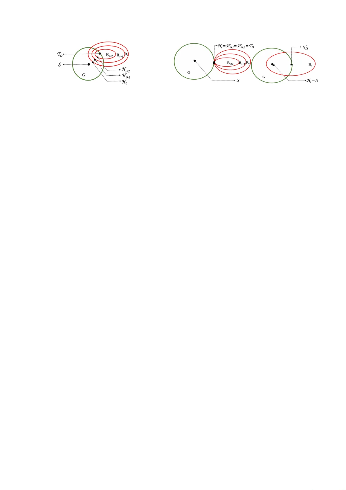
Incremen tal Data Driv en T ransfer Iden tification ⋆ N. Na veen Muk esh a , Debra j Chakrab ort y a a The authors ar e with the Dep artment of Ele ctric al Engine ering, Indian Institute of T e chnolo gy Bomb ay, Mumb ai, India. Abstract W e in tro duce a geometric metho d for online transfer identification of a deterministic linear time-in v ariant system. At the b eginning of the iden tification process, we assume access to abundan t data from a system that is similar, though not iden tical, to the true system. In the early stages of data collection from the true system, the dataset generated is still not sufficien tly informativ e to enable precise identification. Consequen tly , multiple candidate mo dels remain consisten t with the observ ations a v ailable at that p oin t. Our method picks, at each instant, the mo del closest to the similar system that is consisten t with the curren t data. As more data are collected, the proposed mo del gradually mov es aw ay from the initial similar system and ev entually con verges to the true system when the data set grows to b e informative. Numerical examples demonstrate the effectiv eness of the incremen tal transfer iden tification paradigm, where iden tified mo dels with minimal data are used to solv e the p ole placemen t problem. Key wor ds: System identification, linear systems, data-driven con trol, similar systems, transfer learning. 1 In tro duction The first step in traditional con trol engineering prac- tice is to mo del and identify the plan t to b e con trolled. Usually , con trolled exp erimen ts are conducted to ob- tain input–output data, after which mo del parameters are estimated through a v ailable tec hniques [Ljung, 1999, V an Ov erschee and De Mo or, 1996]. Ho wev er, in this framew ork, the data collection pro cess needs to con- tin ue for long enough such that the data set grows to satisfy certain rank conditions [Kata yama, 2005]. More- o v er, larger data sets are necessary to ensure adequate robustness against noise [Pourgholi et al., 2023]. Conse- quen tly , mo del-based controller design can only b e ini- tiated once these conditions are satisfied. In contrast, a gro wing bo dy of recent research on data-driven control [D¨ orfler, 2023, D¨ orfler, 2023] has bypassed the reliance on explicit mo dels b y constructing con trollers directly from recorded data. Ho wev er, ev en in these papers, a fully informative data set is necessary to solve control problems [Celi et al., 2023, De P ersis and T esi, 2019], and the requirement for length y data sets p ersists. In man y practical contexts, suc h prolonged data collection or re- collection can b e b oth inconv enien t and costly . Typi- cal examples include p etro c hemical pro cesses, where the time constan ts are inheren tly large [Chiuso et al., 2007], as w ell as complex, nonlinear, or time-v arying systems ⋆ The material in this paper was partially presented at the 64th IEEE Conference on Decision and con trol (CDC), De- cem b er 10-12, 2025, Rio de Janeiro, Brazil. Email addr esses: nnmukesh@ee.iitb.ac.in (N. Na veen Muk esh), dc@ee.iitb.ac.in (Debra j Chakrab orty). that require p erio dic re-identification to maintain ac- curacy [Lorenzen et al., 2019]. T o address these chal- lenges and accelerate the identification pro cess, a grow- ing b ody of literature [Chakrabarty, 2022, Chakrabarty et al., 2023, Du et al., 2024, Huang et al., 2025, Ke- dia et al., 2024, Ping et al., 2022, 2025, Ric hards et al., 2023, T oso et al., 2023, Xin et al., 2022, 2025, Zhang et al., 2023] advocates the use of previously recorded, abundan t data from a similar system, together with data from the current (online or true) system to be iden tified. This com bination, if done correctly , transfers the kno wl- edge from the similar system to the true system, yield- ing an identified model during the early stages of online data collection, at a p oin t where no unique mo del could ha v e b een obtained using only data from the online/true system. In this pap er, we introduce a no vel framework for suc h tr ansfer identific ation of deterministic systems, whic h guarantees b oth the existence and uniqueness of the iden tified model at eac h stage, and rigorously estab- lishes the conv ergence of these models to the true system as additional data b ecome av ailable. While the literature on data-driven control is extensiv e (e.g., see [Baggio et al., 2021, Berb eric h et al., 2020, Bisoffi et al., 2022, De Persis and T esi, 2019, D¨ orfler et al., 2023, Rueda-Escob edo et al., 2021, V an W aarde et al., 2020] and the references therein), the in te- gration of pre-collected data from a similar system with sparse online measurements has emerged recently [Chakrabart y, 2022, Chakrabart y et al., 2023, Du et al., 2024, Huang et al., 2025, Kedia et al., 2024, Ping et al., 2022, 2025, Ric hards et al., 2023, T oso et al., 2023, Xin et al., 2022, 2025, Zhang et al., 2023]. In [Kedia et al., 2024, T oso et al., 2023, Xin et al., 2022, 2025], data from a similar system was concatenated to the on- line data to enhance noise robustness in least squares, Ba y es ian estimation, and subspace identification set- tings. How ever, it is known that concatenating data from t wo distinct systems may not alwa ys yield consis- tency with an y underlying mo del [Eising et al., 2025]. Ba y es ian meta learning tec hniques were used f or similar ob jectives in [Chakrabart y, 2022, Chakrabarty et al., 2023, Richard s et al., 2023]. Nevertheless, the use of deep neural netw orks introduced significant difficulties in providing rigorous theoretical guarantees. Data from similar systems was utilized to design LQR solutions in [Ba ja j et al., 2025, Guo and P asqualetti, 2025], which ho w ever required to assume additional information suc h as impulse resp onse data from the true system or kno wn p erturbation b ounds on the true parameters. In [Huang et al., 2025, Ping et al., 2022, 2025], transfer iden tification was numerically explored in the context of regression mo dels. T ransfer learning [Zhuang et al., 2020] was systemati- cally introduced in the control domain in [Du et al., 2024] for training across m ultiple systems, though it is based on the assumption that the system parameters share a common column space. In [v an W aarde et al., 2020], a common controller was found for all the systems that are consisten t with the a v ailable (p ossibly non-informativ e) data. Due to the frequen t infeasibility of this approach, [Li et al., 2023] augmen ted the metho d with data from a similar system by constructing a set of systems that w as b oth consistent with the a v ailable online data and within a pre-known distance of the similar system. Ho w- ev er, this metho d required an LMI-based conv ex feasi- bilit y search at eac h step, making it challenging to use in online settings. As opp osed to most of the pap ers cited ab o ve, the geometric metho d of com bining similar and true system data proposed in this paper, guaran tees the existence and uniqueness of an identified mo del at each stage, do es not require to p erform any online optimiza- tion, nor do es it require to tune weigh ting parameters or matrices to balance the con tributions of data from the true system and auxiliary data from similar systems. This simplicit y enhances computational efficiency , mak- ing the proposed approach well-suited for online imple- men tation. In this article, we assume a certain level of confidence in the similar system. This confidence can come from earlier experience with that system or from engineer- ing judgment. F or instance, the similar system ma y b e represented by a high-fidelity computer simulations or ph ysics-based mo dels built from the man ufacturer’s nominal sp ecifications. Although we an ticipate that the true system differs sligh tly from the similar system, w e rely on the similar system until sufficien t evidence is ob- tained to suggest otherwise. T o clarify this framew ork, w e first characterize systems through the subspaces formed b y the data they pro duce [Alsalti et al., 2024, W ang and Meng, 2025], and we quantify how differen t t w o systems are by computing the distances b et ween their corresponding subspaces [Mandolesi, 2019, W edin, 2006]. As stated earlier, when only a short sequence of data from the true system is av ailable up to the present time, there may exist infinitely man y subspaces/systems that are consistent with the observ ed data. Therefore, selecting a single system from this infinite collection is not straightforw ard. How ever, if abundan t data from a similar system are also av ailable, we prop ose a metho d for constructing new subspaces that b oth contain the true system data up to the current instant and remain closest (according to an appropriately defined subspace distance) to the subspace asso ciated with the similar system data. This evolving family of subspaces is then used to estimate (and rep eatedly re-estimate) the sys- tem parameters at every time instan t. Alternatively , these subspaces may be directly utilized to synthesize con trollers through data-driv en tec hniques. Beyond in- tro ducing this new subspace construction sc heme, we pro v e/derive the following: (i) The subspaces computed by the prop osed metho d at eac h time step mov e monotonically (accord- ing to an appropriately defined distance b et ween subspaces) tow ards the unkno wn subspace of the true system as the amount of online data increases and satisfies the standard informativity conditions [De Persis and T esi, 2019, Willems et al., 2005]. (ii) At ev ery time instan t, a unique state-space mo del can alwa ys b e extracted from the constructed sub- space. (iii) The mo del parameters obtained at eac h time step from the corresp onding subspaces conv erge to the actual system parameters once the data becomes informativ e. (iv) The numerical implementation of the prop osed paradigm and its computational complexit y . Finally , with the help of n umerical examples, w e v alidate the theoretical results and demonstrate the practical rel- ev ance of the prop osed approach with online/minimal data. This work extends the results presented in [Mukesh et al., 2025], where the incremental transfer iden tifi- cation paradigm was originally introduced. Ho w ev er, [Muk esh et al., 2025] did not pro vide formal theoretical guaran tees regarding how the accuracy of parameter estimates ev olves as the computed subspaces incre- men tally con verge tow ard the unkno wn true system subspace. W e pro vide these guaran tees here. This paper also includes formal pro ofs of several key theorems and complexit y analysis of the algorithm that w ere omitted in [Mukesh et al., 2025]. F urthermore, several nov el ex- amples are presented to illustrate the effectiv eness and practical relev ance of the prop osed approach. 2 Problem Setup W e b egin b y outlining the preliminaries and form ulating the problem of interest. W e use standard mathematical notations from [Stewart and Sun, 1990] throughout the 2 pap er. 2.1 T rue and similar system 2.1.1 T rue System Our ob jective is to identify the following discrete-time deterministic L TI system: x T ( k + 1) = A T x T ( k ) + B T u T ( k ) , k ∈ { 0 , 1 , . . . } (1) where A T ∈ R n × n and B T ∈ R n × m denote the unknown true system matrices to be determined. W e assume that data collection b egins at time t = 0, and by time t = i , the input–state data of the form { u T ( t ) , x T ( t ) } i t =0 has b een recorded. 2.1.2 Similar System No w, consider a different system having the same input and state dimensions as (1): x S ( k + 1) = A S x S ( k ) + B S u S ( k ) , k ∈ { 0 , 1 , . . . } (2) The degree of similarity is specified in Assumption 1. W e assume that input–state data of sufficien t length (namely N S + 1) from the similar system (2) is a v ailable at time t = 0, i.e., { u S ( τ ) , x S ( τ ) } N s τ =0 is already a v ailable at t = 0. 2.2 Data Matric es Using the a v ailable data till the i th time instan t, the follo wing matrices are defined for the true system, X i − T := h x T (0) x T (1) · · · x T ( i − 1) i ∈ R n × i , X i + T := h x T (1) x T (2) · · · x T ( i ) i ∈ R n × i . (3) The matrix U i − T ∈ R m × i is defined using input data similar to X i − T . F urther, we define the data matrices X − S ∈ R n × N S , U − S ∈ R m × N S , X + S ∈ R n × N S constructed using the a v ailable data from the similar system. F rom (1) and (2), the data matrices ab o ve satisfy the following relations: X + S = [ A S B S ]  X − S U − S  , X i + T = [ A T B T ]  X i − T U i − T  . Define M := 2 n + m , and the com bined data matrix S as follows: S := [ X − S ⊤ U − S ⊤ X + S ⊤ ] ⊤ ∈ R M × N S . (4) Similarly , for the true system, denote the data matrix T i := [ X i − T ⊤ U i − T ⊤ X i + T ⊤ ] ⊤ ∈ R M × i . (5) Define Λ := n + m and Ω := n + m + nm − 1. Assumption 1 The fol lowing ar e assume d: (1) The input { u S ( τ ) } N S τ =0 is p ersistently exciting [De Persis and T esi, 2019, Wil lems et al., 2005] of or der n + 1 . (2) ∥ [ A T B T ] − [ A S B S ] ∥ F ⩽ δ , wher e δ is an unknown (smal l) c onstant, and ∥·∥ F denotes the F r ob enius norm. (3) ( A S , B S ) is c ontr ol lable. (4) L et ∆ A ∈ R n × n , ∆ B ∈ R n × m . Then every system in the set { ( A S + ∆ A, B S + ∆ B ) | ∥ [∆ A ∆ B ] ∥ F ≤ δ } Fig. 1. Illustration of prop osed paradigm is c ontr ol lable. (5) The curr ent time t = i satisfies i ⩽ Ω . (6) Abundant data is available fr om the similar system. i.e., N s >> Ω . It is well established [Willems et al., 2005] that, under these assumptions, rank[ X − S ⊤ U − S ⊤ ] ⊤ = Λ. If we denote the range space of a matrix b y Im( · ) and define S := Im( S ), then dim( S ) = Λ. F urthermore, if we define T i := Im( T i ), it follows that under this setup the true system data T i ma y not satisfy the ab o ve rank condition, i.e., dim( T i ) < Λ for i < Ω. On the other hand, the equality dim( T Ω ) = Λ holds pro vided that a p ersisten tly exciting input sequence { u T ( t ) } Ω t =0 is applied to the true system. Let Gr( k , N ) denote the Grassmannian (the set of all k dimensional linear subspaces of R N ) [Beyn and H ¨ uls, 2024]. Then S , T Ω ∈ Gr(Λ , M ). Remark 1 F r om [Wonham, 1985, The or em 1.3], it is wel l known that if ( A S , B S ) is c ontr ol lable, then ∃ ε such that al l systems in the set { ( A, B ) | ∥ [ A − A S B − B S ] ∥ F ≤ ε } ar e c ontr ol lable. Henc e, if δ ⩽ ε , then statement 4 of Assumption 1 fol- lows dir e ctly. In addition, we note her e that our appr o ach r emains valid even otherwise. However, in that c ase, the identifie d interme diate systems (say ( A i , B i ) ) would not ne c essarily b e c ontr ol lable. 2.3 Pr oblem F ormulation and Pr eliminaries Problem 1 (a) Given T i at time step i , our go al is to identify a mo del  say ( A i , B i )  which is c on- sistent with the data T i and closest (in an appr o- priate sense) to ( A S , B S ) by utilizing the data set { u S ( τ ) , x S ( τ ) } N s τ =0 . (b) As additional data fr om ( A T , B T ) b e c omes available, r e-identify the system at e ach time step to obtain a mor e ac cur ate mo del. W e solve the ab o ve problem by interpreting systems as subspaces and finding the subspace (s a y H i ) containing T i that is closest to, and is of the same dimension as S . W e next recall some preliminaries. Definition 1 (Principal angles and v ectors) [Bj¨ or ck and Golub, 1973] L et A , B denote two subsp ac es of R M with p = dim( A ) , q = dim( B ) and p ⩾ q > 0 . The princip al angles 0 ⩽ θ k ⩽ π 2 for k = 1 , 2 . . . , q is define d r e cursively as fol lows cos θ k = max u ∈A v ∈B u ⊤ v = u ⊤ k v k 3 subje ct to u ⊤ k u j = 0 , v ⊤ k v j = 0 ∀ j = 1 , 2 , . . . , k − 1 , and ∥ u k ∥ 2 = 1 , ∥ v k ∥ 2 = 1 for al l k = 1 , 2 . . . , q . The ve c- tors u 1 , u 2 , . . . , u q , v 1 , v 2 , . . . , v q ar e c al le d the princip al ve ctors. By definition, the principal angles are such that 0 ⩽ θ 1 ⩽ θ 2 ⩽ · · · ⩽ θ q ⩽ π 2 . Definition 2 (Distance betw een subspaces) [Mandolesi, 2019] L et A , B denote two subsp ac es of R M such that dim( A ) ⩽ dim( B ) . The distanc e (maximal angle) b e- twe en the two subsp ac es is define d as, d ( A , B ) := max u ∈A ∥ u ∥ 2 =1 min v ∈B ∥ v ∥ 2 =1 cos − 1 u ⊤ v = θ max (6) wher e θ max denotes the maximum princip al angle b etwe en A and B . The ab o ve notion of distance forms a metric space o ver subspaces of fixed dimensions [Beyn and H¨ uls, 2024]. Note that the notation d ( · , · ) is used throughout the pa- p er without prop er ordering of the subspaces. The cor- rect ordering should b e understo o d from the context. 2.4 F r om State-Sp ac e Mo dels to Subsp ac e R epr esenta- tions Our approac h is illustrated in Fig. 1. By Assumption 1, ( A T , B T ) ∈ { ( A , B ) | ∥ [ A S B S ] − [ A B ] ∥ F ⩽ δ } and this set translates to a set G :=  Im  X − U − X +  | X + = [ A B ] h X − U − i with rank h X − U − i = Λ and ∥ [ A S B S ] − [ A B ] ∥ F ⩽ δ  ⊆ Gr(Λ , M ) This set is marked b y the green circle in Fig. 1. The similar system subspace S is denoted b y a solid dot, and the unknown true system subspace T Ω is denoted by a star. When we ha ve insufficient data (i.e., rank( T i ) < Λ), m ultiple mo dels that describ e the data set exist. This set is given b y Σ i =  ( A , B ) | X i + T = [ A B ]  X i − T U i − T   and ( A T , B T ) ∈ Σ i . Analogous to this set in Gr(Λ , M ) we ha v e the set R i := {H | H ⊇ T i and dim( H ) = Λ } ⊆ Gr(Λ , M ) (mark ed by red ellipse). Note that T Ω ∈ G ∩ R i holds. Due to our said trust in S , we prop ose to c ho ose the subspace H i (mark ed b y a solid square) closest to S but lying inside the red ellipse. The metho d to construct suc h a subspace is describ ed next. Remark 2 We would like to emphasize the fact that the sets r epr esente d by the r e d el lipse and the gr e en cir cle in Fig. 1 ar e pur ely il lustr ative and ar e shown her e to fa- cilitate the e asy interpr etation of our r esults. In gener al, these sets ar e not c onstr aine d to such ge ometric forms. 3 Incremen tal Subspaces W e b egin b y desc ribing how to construct the subspace that is closest to a given subspace (sa y U ) while also con taining a sp ecified vector (say a 1 / ∈ U ). Fig. 2. Closest subspace to U containing the vector a 1 Example 1 Consider a subsp ac e U and a ve ctor a 1 / ∈ U , as shown in Fig. 2, with d ( U, a 1 ) = θ . L et b 1 denote the pr oje ction of a 1 onto U , and define b 2 = a ⊥ 1 ∩ U , wher e ( · ) ⊥ r epr esents the ortho gonal c omplement. F or ve ctors v 1 , . . . , v k , we use ⟨ v 1 , . . . , v k ⟩ to denote their line ar sp an. It fol lows that among al l subsp ac es c ontaining a 1 , the subsp ac e V = ⟨ a 1 , b 2 ⟩ , with d ( U, V ) = d ( U, a 1 ) = θ is the one closest to U . The princip al angles θ i ’s to gether with their asso ciate d princip al ve ctors u i ’s and v i ’s, c or- r esp onding to the subsp ac es U and V , ar e il lustr ate d in Fig. 2. □ W e no w employ this idea to construct subspaces by in- cremen tally combining similar and true system data. De- fine h i :=  x ( i − 1) u ( i − 1) x ( i )  ∈ R M as the v ector containing the data collected from the true system ( A T , B T ) at the i th instan t. Hence, T i = Im( T i ) = Im[ h 1 h 2 · · · h i ] for i = 1 , 2 , . . . , Ω . (7) Next, we present the prop osed formula for incremen tal subspace construction. F or i = 1 , 2 , . . . , Ω, let H i b e defined as follows: H i := T i + ( T ⊥ i ∩ S ) . (8) Clearly , h i ∈ T Ω holds. Also, T i ⊆ T Ω . Definition 3 (P artial orthogonalit y) [Mandolesi, 2019] L et A , B ⊆ R M b e two subsp ac es. A is said to b e p artial ly ortho gonal to B if ∃ an non-zer o ve ctor a ∈ A such that a ⊤ b = 0 ∀ b ∈ B . i.e A ∩ B ⊥  = { 0 } . Additionally , if B is partially orthogonal to A , then the subspaces A and B are said to b e partially orthogonal. In Fig. 2, the subspaces U and V are partially orthogonal as U ∩ V ⊥ = U ⊥ ∩ V = { 0 } holds. Whereas, consider a subspace V 1 := ⟨ a 1 , b 1 ⟩ , then the subspaces U and V 1 are partially orthogonal as U ∩ V ⊥ 1 = ⟨ u 2 ⟩  = { 0 } and U ⊥ ∩ V 1 = U ⊥  = { 0 } holds. Assumption 2 We assume that the subsp ac es S and T Ω ar e not p artial ly ortho gonal. (i.e., ( S ⊥ ∩ T Ω ) = ( T ⊥ Ω ∩ S ) = { 0 } holds) Remark 3 The ab ove assumption is exp e cte d to b e true even though we do not have ful l information or c on- tr ol over the subsp ac e T Ω . It is known that tr ansver- sality of subsp ac es is a generic pr op erty (i.e., any two subsp ac es A , B ⊆ R M would have the pr op erty that dim( A + B ) = min { dim( A ) + dim( B ) , M } hold generi- c al ly) [Wonham, 1985, Se ction 0.16]. Henc e, in our c ase any r andomly chosen S , T would satisfy dim( S + T ⊥ Ω ) = M ( ∵ dim( S ) = Λ , dim( T ⊥ Ω ) = M − Λ) generic al ly. 4 Equivalently, S + T ⊥ Ω = R M and S ⊥ ∩ T Ω = { 0 } hold generic al ly. Similarly, S ∩ T ⊥ Ω = { 0 } is also generic al ly true. Henc e, for any two systems ( A T , B T ) , ( A S , B S ) , the subsp ac es S , T Ω would satisfy Assumption 2 generi- c al ly and henc e no prior verific ation is r e quir e d. Absence of Assumption 2 can lead to the following tw o issues: (1) Necessary dimension for system identification Λ migh t not b e preserved. (2) It ma y not b e feasible to c haracterize a unique sub- space closest (according to the metric in (6)) to the similar system subspace. Example 2 Consider the subsp ac es S = Im h 1 0 0 1 1 0 i , T Ω = Im h 1 0 0 1 − 1 0 i . Note that the subsp ac es S and T Ω ar e p artial ly ortho gonal. A t t = 1 , let T 1 = [ 1 0 − 1 ] ⊤ b e available. Then, T ⊥ i ∩ S = S and H i c onstructe d using the formula in (8) yields H i = R 3 . Cle arly, the ne c essary dimension for system identific ation is not pr eserve d. Next, c onsider the attempt to c onstruct a subsp ac e H i satisfying dim( H i ) = dim( S ) by sele cting a subsp ac e of dimension exactly e qual to dim( S ) − dim( T i ) fr om T ⊥ i ∩S . F or example, cho osing H i = ⟨ T 1 , v ⟩ with v ∈ ( T ⊥ i ∩ S ) ) r esults in infinitely many p ossible choic es for H i . Henc e, the primary obje ctive of ensuring mo del uniqueness is not achieve d. □ W e now pro ceed to demonstrate certain fundamental prop erties of the constructed subspaces H i . 3.1 Pr op erties of H i with fixe d data size The follo wing result characterizes the dimension of H i ’s constructed in (8) and ensures that the necessary dimen- sions required for the unique iden tification of the system are preserved. Theorem 1 (Dimension preserv ation) L et H i b e define d as in (8) . Then, under Assumption 2, dim( H i ) = Λ ∀ i ⩽ Ω holds. PR OOF. Consider T i as defined in (7). dim( S ∩ T ⊥ i )= M − dim( S ∩ T ⊥ i ) ⊥ ( ∵ S ∩ T ⊥ i ⊆ R M ) = M − dim( S ⊥ + T i ) = M − (dim S ⊥ + dim T i − dim( S ⊥ ∩ T i )) = dim S − dim T i . (9) The last equality follows since dim S ⊥ = M − dim S and dim( S ⊥ ∩ T i ) = 0 holds. The latter one holds due to our assumption of subspaces not b eing partially orthogonal, i.e., S ⊥ ∩ T Ω = { 0 } holds, and hence, S ⊥ ∩ T i = { 0 } holds as T i ⊆ T Ω . Now since H i = T i + ( S ∩ T ⊥ i ), dim H i = dim T i + dim( S ∩ T ⊥ i ) ( ∵ T i ⊥ ( S ∩ T ⊥ i )) = dim S (from (9)) . The ab o ve relation holds for all i ⩽ Ω. By statement 1 of Assumption 1 it follows that dim( S ) = Λ and hence dim( H i ) = Λ for all i ⩽ Ω. ■ It follows directly that whenever sufficient data from the actual system is av ailable (i.e., rank( T i ) = Λ), the subspaces H i constructed in (8) conv erge to T Ω . Corollary 1 L et Assumption 2 hold. Then, the fol low- ing ar e true: (i) If dim( T i ) = Λ , then H i = T Ω . (ii) If dim( T i ) = 0 , then H i = S . PR OOF. F rom (9), w e get dim( S ∩ T ⊥ i ) = 0 when dim( T i ) = Λ. Therefore, (8) b ecomes H i = T i + 0 = T Ω (as T i = T Ω when dim( T i ) = Λ). Statemen t (ii) also follo ws similarly . ■ Remark 4 F r om (8) and (9) , we infer that the sub- sp ac es H i p ossess an intrinsic pr op erty: at the initial stages, they r ely mor e he avily on similar system data, sinc e dim  T ⊥ i ∩ S  > dim( T i ) . However, as mor e sys- tem data b e c omes available, the r elianc e on similar sys- tem data de cr e ases, b e c ause dim  T ⊥ i ∩ S  < dim( T i ) . This c onstitutes a key fe atur e of the c onstruction: the subsp ac es natur al ly adjust their dep endenc e on similar system data without the ne e d to intr o duc e explicit weight p ar ameters [Huang et al., 2025, Ping et al., 2022, 2025, Xin et al., 2025, Zhang et al., 2023]. Denote σ min ( · ) to b e the minimum singular v alue of a matrix. The following lemmas will help us pro ve our main results. Lemma 1 L et A , B ⊆ R M b e two subsp ac es and Q A , Q B b e matric es use d to r epr esent their orthonormal b asis r e- sp e ctively. L et D ⊆ A ∩ B ⊥ and Q D b e a matrix c ontain- ing orthonormal ve ctors that sp an D . Define C = B ⊕ D , and let dim( A ) ⩾ dim( C ) . F urther, assume that B is not p artial ly ortho gonal to A . Then, (i) σ min ( Q ⊤ A Q B ) = σ min ( Q ⊤ A [ Q B Q D ]) or e quiva- lently d ( A , B ) = d ( A , C ) . (ii) If D = A ∩ B ⊥ , then dim( C ) = dim( A ) and the subsp ac e C is unique. PR OOF. See App endix. ■ In the following lemma, we prov e the conv erse statemen t of Lemma 1. Lemma 2 Consider thr e e subsp ac es A , B , C ⊆ R M and let B ⊆ C . If d ( A , B ) = d ( A , C ) , then ∃ a subsp ac e D ⊆ A ∩ B ⊥ such that C = B ⊕ D with dim( D ) = dim( A ∩ C ) − dim( A ∩ B ) . PR OOF. See App endix. ■ The follo wing theorem ensures that the subspaces H i ’s constructed in (8) are closest to S among all subspaces that contain T i at the i -th instant. Theorem 2 (Nearest to S and consisten t with data) L et T i , H i b e define d as in (7) and (8) r esp e ctively. L et As- sumption 2 hold and let dim( T i ) = i ∀ i ∈ { 1 , 2 , . . . , Λ } . Then, (i) d ( S , H i ) = d ( S , T i ) (ii) d ( S , H i ) < d ( S , e H i ) for any subsp ac e e H i  = H i such that T i ⊆ e H i and dim( e H i ) = Λ . 5 PR OOF. As H i , T i are related by (8), (i) follows from Lemma 1. F rom Lemma 1 and Lemma 2, w e conclude that for all subspaces D ⊈ A ∩ B ⊥ , we get d ( A , B ) < d ( A , C ) where C = B ⊕ D . Hence, d ( S , H i ) < d ( S , e H i ). ■ By the ab ov e theorem, it is now clear that our choice of subspace H i (mark ed by a solid square) in Fig. 1 is the closest to S and consisten t with the data T i (lying inside the red ellipse). Theorem 3 L et T i , H i b e define d as in (7) and (8) , r esp e ctively. L et Assumption 2 hold and dim( T i ) = i ∀ i ∈ { 1 , 2 , . . . , Λ } . Then, (i) d ( T Ω , H i ) = d ( T Ω , T ⊥ i ∩ S ) . (ii) d ( T Ω , H i ) < d ( T Ω , e H i ) for any subsp ac e e H i  = H i such that ( T ⊥ i ∩ S ) ⊆ e H i . PR OOF. By Lemma 1, it follows that d ( T Ω , T ⊥ i ∩ S ) = d ( T Ω , ( T ⊥ i ∩ S ) + T i ) as T i ⊆ T Ω and T i ⊥ ( T ⊥ i ∩ S ). Next to prov e (ii), note that H i can b e written as H i = ( T ⊥ i ∩ S ) + (( T ⊥ i ∩ S ) ⊥ ∩ T Ω ) , (10) as (( T ⊥ i ∩ S ) ⊥ ∩ T Ω ) = (( T i + S ⊥ ) ∩ T Ω ) = T i ( ∵ S ⊥ ∩ T Ω = { 0 } b y Assumption 2). Comparing (10) and (8), then by Theorem 3 statement (ii), (ii) follows. ■ The ab o v e theorem says that H i ’s constructed as in (8) is the closest to T Ω among all subspaces containing ( T ⊥ i ∩ S ). Next, w e study the monotonic properties of the distance betw een H i and the subspaces S and T Ω as the av ailability of data increases. 3.2 Pr op erties of H i under incr e asing data availability The following theorem establishes the first monotonicity prop ert y relating the distances betw een the constructed subspaces H i and the similar system subspace S . Theorem 4 (Monotonic div ergence from S ) L et T i , H i b e define d as in (7) and (8) r esp e ctively. L et As- sumption 2 hold and let dim( T i ) = i ∀ i ∈ { 1 , 2 , . . . , Λ } . Then, (i) d ( S , H i ) < d ( S , H j ) ∀ H i  = H j for i < j ⩽ Λ . (ii) d ( S , H i ) < d ( S , T Ω ) ∀ i ∈ { 1 , 2 , . . . , Λ } such that H i  = T Ω . PR OOF. T o prov e (i), w e compare H j = T j + ( T ⊥ j ∩ S ) and H i = T i + ( T ⊥ i ∩ S ) where i < j . Under the assumption dim( T i ) = i , T j ⊃ T i and ( T ⊥ j ∩ S ) ⊂ ( T ⊥ i ∩ S ) holds, where the latter inclusion holds because T ⊥ j ⊂ T ⊥ i and dim( T ⊥ j ∩ S ) = Λ − j < dim( T ⊥ i ∩ S ) = Λ − i for i < j . Then ∃ a subspace F of dimension j − i such that ( T ⊥ i ∩ S ) = ( T ⊥ j ∩ S ) + F . Hence, H i can b e rewritten as H i = T i + ( T ⊥ j ∩ S ) + F . Similarly , H j = T i + ⟨ h i +1 , . . . , h j ⟩ + ( T ⊥ j ∩ S ) , (11) where T j = T i + ⟨ h i +1 , . . . , h j ⟩ due to (7). It is easy to sho w that, when H i  = H j , F  = ⟨ h i +1 , . . . , h j ⟩ . d ( S , H i ) ( a ) = d ( S , T i ) ( b ) = d ( S , T i + ( T ⊥ j ∩ S )) < d ( S , T i + ( T ⊥ j ∩ S ) + ⟨ h i +1 , . . . , h j ⟩ ) = d ( S , H j )(from (11)) Equalit y ( a ) is due to Theorem 2 statement (i) and equal- it y ( b ) holds due to Lemma 1 as ( T ⊥ j ∩ S ) ⊂ ( T ⊥ i ∩ S ). The inequality holds due to Lemma 2 as ⟨ h i +1 , . . . , h j ⟩ ⊈ ( T ⊥ i ∩ S ). d ( S , H i ) < d ( S , T Ω ) also follows in a similar wa y . ■ As a direct consequence of the ab ov e theorem, we obtain, d ( S , H 0 ) | {z } =0 < d ( S , H 1 ) < · · · < d ( S , H Λ − 1 ) < d ( S , H Λ ) | {z } = d ( S , T Ω ) assuming that a new direction of T Ω is obtained at each stage. The ab o ve theorem implies that, as additional data b ecome a v ailable, the prop osed model sequentially div erges from the similar system. In the follo wing theorem, it will be shown that the pro- p osed mo del shifts closer to the true system subspace sequen tially . Theorem 5 (Monotonic con v ergence to T Ω ) L et T i , H i b e define d as in (7) and (8) , r esp e ctively. L et Assumption 2 hold and dim( T i ) = i ∀ i ∈ { 1 , 2 , . . . , Λ } . Then, (i) d ( T Ω , H i ) > d ( T Ω , H j ) ∀ H i  = H j for i < j ⩽ Λ . (ii) d ( T Ω , S ) > d ( T Ω , H i ) ∀ i ∈ { 1 , 2 , . . . , Λ } such that H i  = T Ω . PR OOF. As shown in the pro of of Theorem 4, we can write H i = T i + ( T ⊥ j ∩ S ) + F , H j = T i + ⟨ h i +1 , . . . , h j ⟩ + ( T ⊥ i ∩ S ) for i < j and eviden tly , when H i  = H j , F  = ⟨ h i +1 , . . . , h j ⟩ . Then, d ( T Ω , H j ) ( a ) = d ( T Ω , T ⊥ j ∩ S ) ( b ) = d ( T Ω , ( T ⊥ j ∩ S ) + T i ) < d ( T Ω , ( T ⊥ j ∩ S ) + T i + F ) = d ( T Ω , H i ) . (12) Here ( T ⊥ j ∩ S ) ⊥ = T j + S ⊥ and hence, ( T ⊥ j ∩ S ) ⊥ ∩ T Ω = T j as S ⊥ ∩ T Ω = { 0 } due to Assumption 2. Equality ( a ) in (12) is due to Theorem 3 statement (i) and equality ( b ) holds due to Lemma 1 as T i ⊂ T j = ( T ⊥ j ∩ S ) ⊥ ∩ T Ω . The inequalit y in (12) follo ws due to Lemma 2, as F ⊈ T j . The last equality in (12) follows since H i = T i + ( T ⊥ j ∩ S ) + F . One can show d ( T Ω , S ) > d ( T Ω , H i ) using similar argu- men ts and hence is omitted. ■ As a consequence of abov e theorem, we hav e, d ( T Ω , S ) > d ( T Ω , H 1 ) > · · · > d ( T Ω , H Λ − 1 ) > d ( T Ω , H Λ ) = 0 , assuming that w e get a new direction of T Ω at eac h stage. Fig. 3 illustrates the v ariation of d ( S , H i ) and d ( T Ω , H i ) 6 Fig. 3. V ariation of d ( S , H i ) and d ( T Ω , H i ) with increasing i . Note that, as i increases, d ( S , H i ) in- creases according to Theorem 4 and d ( T Ω , H i ) decreases according to Theorem 5. W e emphasize that the red el- lipse and the green circle in Fig. 3 are purely illustrativ e in nature, included only to support the clear interpreta- tion of our result. 3.3 Sp e cial c ases arising fr om the pr op ose d fr amework Next, w e see some special cases of our setup. The follow- ing result deals with a special case when H i constructed matc hes with T Ω at some in termediate stage when we ha v e insufficien t data. Lemma 3 L et dim( T i ) = i ∀ i ∈ { 1 , 2 , . . . , Λ } , let As- sumption 2 hold and T i  = T Ω . Then, the fol lowing ar e e quivalent (1) T ⊥ i ∩ S = T ⊥ i ∩ T Ω . (2) H i = T Ω . (3) d ( H i , S ) = d ( T Ω , S ) . (4) d ( T i , S ) = d ( T Ω , S ) . PR OOF. (1) ⇒ (2) When T ⊥ i ∩ S = T ⊥ i ∩ T Ω , clearly w e ha v e H i ⊆ T Ω as ( T ⊥ i ∩ S ) ⊆ T Ω holds in addition to T i ⊆ T Ω . Also as dim( H i ) = dim( T Ω ), we get H i = T Ω . (2) ⇒ (3) follows directly . (3) ⇒ (4) follows from Theorem 2, statement (i). (4) ⇒ (1) By Lemma 2, ∃ a subspace F such that T Ω = T i + F such that F ⊆ ( S ∩ T ⊥ i ). But dim( F ) = dim( S ∩ T ⊥ i ) and hence F = ( S ∩ T ⊥ i ). Therefore, T Ω = T i + ( S ∩ T ⊥ i ). No w, ( T ⊥ i ∩ T Ω ) = ( T ⊥ i ∩ S ) as ( T ⊥ i ∩ T i ) = { 0 } . ■ The illustration of the ab ov e scenario is sho wn in Fig. 4a. In that case, all subsequently constructed H i ’s will be iden tical and equal to T Ω . The following theorem guar- an tees that. Theorem 6 L et dim( T i ) = i ∀ i ∈ { 1 , 2 , . . . , Λ } and let Assumption 2 hold. F or some T i , if the c onditions in L emma 3 holds, then H j = T Ω ∀ j satisfying i ⩽ j ⩽ Λ . PR OOF. If the conditions in Lemma 3 holds, then H j = T j + ( T ⊥ j ∩ S ) ⊆ T Ω as ( T ⊥ j ∩ S ) ⊆ ( T ⊥ i ∩ S ) = ( T ⊥ i ∩ T Ω ) ⊆ T Ω holds for i ⩽ j and T j ⊆ T Ω holds by def- inition. But dim( H j ) = dim( T Ω ) and hence H j = T Ω . ■ The following theorem deals with another special case when the H i constructed at the i th time instan t ( i < Ω) matc hes with S . Theorem 7 L et Assumption 2 hold. If T i ⊆ S , then H i = S . (a) (b) Fig. 4. Sp ecial cases PR OOF. When T i ⊆ S , clearly we hav e H i ⊆ S as ( T ⊥ i ∩ S ) ⊆ S also holds. Also as dim( H i ) = dim( S ), w e get H i = S . ■ The inclusion T i ⊆ S means that the similar system is also consisten t with the dataset T i . In this case, the red ellipse contains the solid dot. (See Fig. 4b) Hence, the solid dot and solid square coincide in this case (i.e., H i = S ). 4 F rom Subspace Represen tations to State- Space Models In this section, w e fo cus on iden tifying a state-space mo del from the subspace H i constructed in accordance with (8), and establish the existence and uniqueness of the identified mo del. 4.1 Existenc e and uniqueness of ( A i , B i ) Recall that, H i ’s are created in (8) as a sum of tw o sep- arate subspaces T i and ( T ⊥ i ∩ S ). Ho wev er, if we add t w o arbitrary subspaces in general, then while the com- bined subspace might ha ve adequate dimension, no sys- tem might exist that can produce data consistent with the combined subspace. Example 3 Consider the system x ( k + 1) = ax ( k ) + bu ( k ) wher e a, b ∈ R . Supp ose the data set T 1 =  x (0) u (0) x (1)  = h 1 1 2 i is available. Sinc e rank( T 1 ) = 1 < 2 we c annot uniquely identify ( a, b ) fr om just T 1 . Supp ose we r an- domly c omplete T 1 to e H 1 = h 1 1 1 1 2 1 i . Cle arly no ( a, b ) p airs exist which ar e c onsistent with a + b = 2 and a + b = 1 simultane ously. □ The next theorem guaran tees that w e are assured of a unique system  denoted b y ( A i , B i )  consisten t with any basis H i of H i constructed according to (8). Define any H i ∈ R M × Λ suc h that Im( H i ) = H i . F urther partition H i = [ X − i ⊤ U − i ⊤ X + i ⊤ ] ⊤ (13) suc h that X − i ∈ R n × Λ , U − i ∈ R m × Λ , X + i ∈ R n × Λ . Then, the following result holds, Theorem 8 (Existence and uniqueness of ( A i , B i ) ) L et dim( T i ) = i ∀ i ∈ { 1 , 2 , . . . , Λ } . Then, ther e exists an unique ( A i , B i ) p air that satisfies X + i = A i X − i + B i U − i , wher e X − i , U − i , X + i ar e define d as in (13) . 7 PR OOF. First, we pro v e the theorem for a sp e- cific c hoice of H i . Consider T i ∈ R M × i as defined in (5). Let S i ∈ R M × (Λ − i ) b e such that its columns forms a basis for T ⊥ i ∩ S . Partition the matrix S i as S i =  e X −⊤ i e U − ⊤ i e X + ⊤ i  ⊤ where e X − i ∈ R n × (Λ − i ) , e U − i ∈ R m × (Λ − i ) , e X + i ∈ R n × (Λ − i ) . Clearly , any suc h partition automatically satisfy the relations X i + T = [ A T B T ]  X i − T U i − T  , and e X + i = [ A S B S ]  e X − i e U − i  . De- note Rowsp( · ) to denote the row span of a matrix. There- fore, Rowsp( X i + T ) ⊆ Ro wsp  X i − T U i − T  , Rowsp( e X + i ) ⊆ Ro wsp  e X − i e U − i  holds. Since rank( T i ) = i and rank( S i ) = Λ − i , it follows that rank  X i − T U i − T  = i and rank  e X − i e U − i  = Λ − i . Next define H oi = [ T i S i ]. Clearly Im [ T i S i ] = H i from (8). Claim: Im  X i − T U i − T  ∩ Im  e X − i e U − i  = { 0 } . W e pro ve the ab ov e claim by contradiction. Supp ose ∃ x ∈ R Λ suc h that x ∈ Im  X i − T U i − T  ∩ Im  e X − i e U − i  and x  = 0, then  x x T  ∈ T i ,  x x S  ∈ ( T ⊥ i ∩ S ) where x T := [ A T B T ] x , x S := [ A S B S ] x . But, [ x ⊤ x ⊤ T ]  x x S  = 0 as T i ⊥ ( T ⊥ i ∩ S ). Hence, x ⊤ x + x ⊤ [ A T B T ] ⊤ [ A S B S ] x = 0. i.e., x ⊤  I Λ + [ A T B T ] ⊤ [ A S B S ]  x = 0 must b e true for an y ( A T , B T ), ( A S , B S ) pair. Therefore, x = 0. Con- tradiction. Hence, rank  X i − T e X − i U i − T e U − i  = Λ. Also as rank( H 0 i ) = Λ, Ro wsp h X i + T e X + i i ⊆ Rowsp  X i − T e X − i U i − T e U − i  is true. Hence, an unique ( A i , B i ) satisfying h X i + T e X + i i = [ A i B i ]  X i − T e X − i U i − T e U − i  exists. It is now easy to argue that any matrix satisfying Im( H i ) = H i partitioned as in (13) is suc h that rank h X − i U − i i = Λ and an unique ( A i , B i ) exists. ■ By the ab o ve theorem, the unique system consisten t with the data in (13) is determined as [De P ersis and T esi, 2019]: [ A i B i ] = X + i h X − i U − i i † . (14) Example 4 L et the data matric es S = h 1 0 0 1 0 . 7 0 . 7 i , T 1 = h 1 1 1 i b e available fr om a system with m = n = 1 . F r om the data set S , the similar system c an b e uniquely identifie d Fig. 5. Graphical illustration of Example 4 as ( A S , B S ) = (0 . 7 , 0 . 7) . Wher e as, c orr esp onding to T 1 , the set of al l c onsistent systems w ith the data is given by Σ 1 = { ( a, b ) | a + b = 1 wher e a, b ∈ R } . Note that Σ 1 is an unb ounde d set and is denote d by the r e d line in Fig. 5. The unknown true system ( A T , B T ) c an lie anywher e on this line. Her e, T ⊥ i ∩ S = ⟨ h 1 − 1 0 i ⟩ (shown by blue line). Henc e, H i = ⟨ h 1 1 1 i , h 1 − 1 0 i ⟩ and the c orr esp onding system is ( A i , B i ) = (0 . 5 , 0 . 5) . □ The follo wing illustrates the fact that appending data from the similar system in a wa y that guaran tees the existence of a system migh t result in systems ( A i , B i ) that are far from the similar system, the true system. Example 5 Consider the same data matric es S , T 1 as in Example 4. Supp ose we r andomly c omplete T 1 to e H 1 = h 1 1 . 09302 1 1 1 1 . 4651 i wher e h 1 . 09302 1 1 . 4651 i ∈ Im( S ) . A lso, her e Rowsp[ 1 1 . 4651 ] ⊆ Rowsp[ 1 1 . 09302 1 1 ] and rank( e H 1 ) = Λ and henc e a unique system c orr esp onding to e H 1 exists and the unique system is ( e A 1 , e B 1 ) = (5 , − 4) . But note that ( e A 1 , e B 1 ) is far fr om b oth ( A S , B S ) and ( A T , B T ) . Henc e, we c an infer that c ombining data fr om similar systems in an arbitr ary way would not b e b eneficial. □ T o summarize, the subspaces H i , constructed with re- sp ect to the metric defined in (6), satisfy the follo w- ing prop erties: (i) Dimension preserv ation (Theorem 1) (ii) Minimizes deviation from the similar system (The- orem 2) (iii) Monotonic divergence from similar system (Theorem 4, statement (i)) (iv) Monotonic conv ergence to true system (Theorem 5, statemen t (i)) (v) Eac h con- structed H i lies closer to T Ω than S do es to T Ω . (Theo- rem 5, statement (ii)) (vi) H i ’s conv erge to T Ω . (Corol- lary 1) (vii) Intermediate system identification (Theo- rem 8). 4.2 Identific ation of Autonomous systems One of the main assumptions of our w ork is that w e ha v e a fully informative dataset from a similar system a v ailable. i.e., dim( S ) = Λ. But, for autonomous sys- tems, since the input comp onen t is zero, we would ha ve dim( S ) < Λ. Ho wev er, with slight mo difications to the constructed data matrices, our approach can also b e used for incremen tally identifying autonomous systems. Next, w e will show ho w our approach can be applied for 8 autonomous systems. Consider T rue system: x T ( k + 1) = A T x T ( k ) , k ∈ { 0 , 1 , . . . } Similar system: x S ( k + 1) = A S x S ( k ) , k ∈ { 0 , 1 , . . . } The data matrices X − S ∈ R n × N s , X + S ∈ R n × N s whic h are defined as in (3) are known to be av ailable. Here, the ma- trices S , T i are defined as S := [ X − S ⊤ X + S ⊤ ] ⊤ ∈ R 2 n × N S , T i := [ X i − T ⊤ X i + T ⊤ ] ⊤ ∈ R 2 n × i . Here, it is assumed that the similar system data satisfies rank( X − S ) = n . This condition ensures that the underlying autonomous sys- tem is uniquely iden tified. It follo ws that dim( S ) = n , as Ro wsp( X + S ) ⊆ Ro wsp( X − S ). F or this case to o, the H i ’s constructed from S , T i as in (8) inherits all the prop- erties discussed in Section 3. Define H i ∈ R 2 n × n suc h that Im( H i ) = H i . F urther partition H i = [ X − i ⊤ X + i ⊤ ] ⊤ suc h that X − i ∈ R n × n , X + i ∈ R n × n . The unique sys- tem identified (say A i ) identified from H i is given by A i = X + i ( X − i ) † . 5 Con vergence of parameters In this section, w e study how the con vergence prop erties of the H i ’s translate to those of the system parameters ( A i , B i ) that are identified using the H i ’s. W e inv estigate the conv ergence of ( A i , B i ) computed from (14) as H i ’s gets computed from (8) at time step i . More precisely , w e inv estigate the dep endencies b et w een (i) d ( H i , T Ω ) and    b H i − b T    F for appropriately c hosen basis b H i and b T , and (ii)    b H i − b T    F and ∥ [ A i B i ] − [ A T B T ] ∥ F where ( A i , B i ) and ( A T , B T ) are estimated from the ma- trices b H i and b T respectively . The following example illustrates the fact that mono- tonicit y in distance betw een subspaces do esn’t necessar- ily translate to monotonicit y in distance b et w een sys- tems represented by state space matrices. Example 6 Consider the data sets D 0 = h 1 0 0 1 1 1 i , D 1 = h 1 0 0 1 1 . 0149 1 . 0619 i , D 2 = h 1 0 0 1 1 . 0268 1 . 0633 i , which ar e c ol le cte d fr om differ ent systems with m = n = 1 . F or i = 1 , 2 , 3 , let D i := Im( D i ) . Her e, d ( D 0 , D 1 ) = 0 . 0257 > d ( D 0 , D 2 ) = 0 . 0252 . It is e asy to se e that al l the data sets D i ’s ar e informa- tive for identific ation [van Waar de et al., 2020]. F or i = 0 , 1 , 2 , if we use ( a i .b i ) to denote the c orr esp onding sys- tem identifie d fr om D i , then ( a 0 , b 0 ) = (1 , 1) , ( a 1 , b 1 ) = (1 . 0149 , 1 . 0169) and ( a 2 , b 2 ) = (1 . 0268 , 1 . 0633) . Her e, ∥ [ a 0 b 0 ] − [ a 1 , b 1 ] ∥ F | {z } =0 . 0637 < ∥ [ a 0 b 0 ] − [ a 2 b 2 ] ∥ F | {z } =0 . 0687 . Though D 2 is closer to D 0 in subsp ac e metric than D 1 , the same is not true in state sp ac e metric. □ Recall that, if dim( A ∩ B ) = i , then θ 1 = θ 2 = · · · = θ i = 0 and the corresp onding principal vectors satisfy u k = v k and u k ∈ ( A ∩ B ) where k = 1 , . . . , i [W edin, 2006]. In Fig. 2, note that dim( U ∩ V ) = 1 and hence one principal angle θ 1 = 0. The following observ ation is used in our subsequent results. Lemma 4 Assume that dim( T i ) = i ∀ i ∈ { 1 , 2 , . . . , Λ } . Then, (1) The p air ( S , H i ) has at le ast Λ − i zer o princip al angles and at most i non-zer o princip al angles. (2) The p air ( T Ω , H i ) has at le ast i zer o princip al angles and at most Λ − i non-zer o princip al angles. PR OOF. Note that from (8), w e get S ∩ H i = ( S ∩ T i ) + ( T ⊥ i ∩ S ). Assuming dim( T i ) = i , it follo ws that, dim( S ∩ H i ) ⩾ dim( T ⊥ i ∩ S ) = Λ − i . As dim( S ∩ H i ) is at least Λ − i , we ha ve at least Λ − i principal angles to b e zero for the pair ( S , H i ). As, dim S = dim H i = Λ, Λ principal angles are defined for the pair of subspaces ( S , H i ), and hence at most i principal angles w ould b e non-zero for the pair ( S , H i ). Statemen t (2) follows in a similar wa y . ■ 5.1 Bounding    b H i − b T    F ab ove by a function of d ( H i , T Ω ) Next, we prop ose a metho d, based on [Bj¨ orck and Golub, 1973, Theorem 1], for choosing a basis for H i and T Ω . Let Q T , Q i ∈ R M × Λ b e matrices containing orthonormal v ectors that span T Ω , H i resp ectiv ely . Obtain the SVD of Q ⊤ T Q i as Q ⊤ T Q i = U Σ V ⊤ , where U, Σ , V ∈ R Λ × Λ . Define, b T := Q T U, b H i := Q i V . (15) In the ab ov e equation, b T , b H i ∈ R M × Λ con tains principal v ectors of the pair ( T Ω , H i ) and is such that Im( b T ) = T Ω , Im( b H i ) = H i . In a similar wa y , for the pair ( S , H i ), we define matri- ces e S , e H i ∈ R M × Λ con taining the corresp onding prin- cipal v ectors. The following lemma relates the distance b et ween the matrices b T , b H i with distance b et ween the subspaces T Ω , H i . Lemma 5 L et b T , b H i b e define d as in (15) . Assume that dim( T i ) = i ∀ i ∈ { 1 , 2 , . . . , Λ } . Then,    b H i − b T    F ⩽ 2 √ Λ − i sin  d ( T Ω , H i ) 2  . A lso,    e H i − e S    F ⩽ 2 √ i sin  d ( S , H i ) 2  holds. PR OOF. Let h ( k ) T , h ( k ) i ∈ R M b e v ectors used to denote the k th column of b T , b H i resp ectiv ely . Then,    h ( k ) i − h ( k ) T    2 2 = 4 sin 2  θ k 2  See Pro of of Lemma 8 in [Alsalti et al., 2024]. ! where θ k is the corresp onding principal angle b et ween the principal vectors h ( k ) i , h ( k ) T . Hence, 9    b H i − b T    F = v u u t Λ X k =1    h ( k ) i − h ( k ) T    2 2 = v u u t Λ X k =1 4 sin 2  θ k 2  =2 v u u t Λ X k = i +1 sin 2  θ k 2  By Lemma 4, at least i principal angles are zero. ! ⩽ 2 q (Λ − i ) sin 2  θ Λ 2  ∵ θ 1 ⩽ θ 2 ⩽ · · · ⩽ θ Λ [Bj¨ orc k and Golub, 1973] ! =2 √ Λ − i sin  d ( T Ω , H i ) 2  ( ∵ d ( T Ω , H i )= θ Λ from (6)) The bound for    e H i − e S    F is deriv ed in a similar w ay . ■ Note that, the bound for    b H i − b T    F decreases with in- crease in i b ecause H i gets closer to T Ω and so the ma- trix b H i also mo ves closer to b T . When d ( T Ω , H i ) = 0, the righ t hand side b ecomes zero and b H i exactly matches b T . In contrast, the b ound for    e H i − e S    F increases as i increases. This is b ecause the subspace H i relies more on the similar system data initially , and hence e H i is also initially closer to e S . As H i deviates from S , the matrix e H i also mov es farther from e S . 5.2 Bound on r elative deviation of ( A i , B i ) fr om ( A T , B T ) Next, w e aim to in vestigate the conv ergence of ∥ [ A i B i ] − [ A T B T ] ∥ F . Let the matrices b T , b H i ∈ R M × Λ b e partitioned as follo ws: b T =  b X −⊤ T b U −⊤ T b X + ⊤ T  ⊤ , b H i =  b X − ⊤ i b U −⊤ i b X + ⊤ i  ⊤ where b X − T , b X + T , b X − i , b X + i ∈ R n × Λ and b U − T , b U − i ∈ R m × Λ . Let δ b X − i := b X − i − b X − T , δA i := A i − A T , δ b X + i := b X + i − b X + T , δ B i := B i − B T , δ b U − i := b U − i − b U − T . Then, b y Theorem 8, b X + i = A i b X − i + B i b U − i holds and equiv alen tly w e can write b X + T + δ b X + i = [ A T + δ A i B T + δ B i ]  b X − T + δ b X − i b U − T + δ b U − i  . (16) Define: n 1 :=      δ b X − i δ b U − i      F ,n 2 : =    δ b X + i    F , ν 1 :=      b X − T b U − T      F , ν 2 : =    b X + i    F . (17) Denote κ 2 ( · ) to b e the 2 condition n um b er of a matrix. The follo wing lemma b ounds the magnitude of relativ e deviation betw een ( A i , B i ), ( A T , B T ) caused as the data matrices  b X − T b U − T  , b X + T deviate to  b X − i b U − i  , b X + i resp ectiv ely . Lemma 6 ∥ [ δ A i δ B i ] ∥ F ∥ [ A i B i ] ∥ F ⩽ κ 2  b X − T b U − T   n 1 ν 1 + n 2 ν 2 + n 1 n 2 ν 1 ν 2  (18) PR OOF. Applying the result of [W atkins, 2004, The- orem 2.3.8] row-wise b y comparing b X + T = A T b X − T + B T b U − T and (16), and b y relating it with the F robenius norm w e get the desired result. ■ Next, we combine Lemma 5 and Lemma 6 to characterize the con vergence of ( A i , B i ) in terms of th e subspace dis- tance d ( H i , T Ω ). First, we state an in termediate lemma required to prov e the main result in Theorem 9. Lemma 7 Consider a subsp ac e V ⊆ R n , with dim( V ) = q . L et Q A , Q B ∈ R n × q denote matric es c ontain- ing orthonormal c olumns that sp an V . Partition Q A = h A 1 A 2 i , Q B = h B 1 B 2 i wher e A 1 , B 1 ∈ R q × q and A 2 , B 2 ∈ R ( n − q ) × q . Then, ∥ B k ∥ F = ∥ A k ∥ F for k = { 1 , 2 } . Also, if A 1 , B 1 ar e invertible, then we have κ 2 ( A 1 ) = κ 2 ( B 1 ) . PR OOF. See App endix. ■ 5.3 Bound on System Identific ation Err or as a function of d ( H i , T Ω ) Next, w e state the main result characterizing the error in iden tified parameters at time step i . Recall the definition of h i from (7). Theorem 9 Consider the notations as in (16) and (17) . Assume that dim( T i ) = i ∀ i ∈ { 1 , 2 , . . . , Λ } . Then the fol lowing ine quality holds: ∥ [ δ A i δ B i ] ∥ F ∥ [ A i B i ] ∥ F ⩽ γ κ 2  b X − T b U − T   1 ν 1 + 1 ∥ h b ∥ 2 + γ ν 1 ∥ h b ∥ 2  (19) wher e γ := 2 √ Λ − i sin  d ( T Ω , H i ) 2  , h b ∈ R n is define d to b e the last n c omp onents of a unit ve ctor in dir e ction of h 1 . PR OOF. First, we aim to b ound the quantities n 1 , n 2 in (17). Note that the matrices  δ b X − i δ b U − i  , δ b X + i b oth are sub-matrices of b T − b H i . Hence, by Lemma 5, { n 1 , n 2 } ⩽    b T − b H i    F ⩽ 2 √ Λ − i sin  d ( T Ω , H i ) 2  , (20) where n 1 , n 2 are defined as in (17). Next, w e aim to b ound 1 ν 2 in (18). Recall h 1 in (7). Let b h 1 denote a unit v ector in direction of h 1 and is partitioned as b h 1 = h h a h b i with h a ∈ R Λ and h b ∈ R n . Note that, b h 1 ∈ T i , as h 1 ∈ T i holds ∀ i ∈ { 1 , 2 , . . . , Λ } . Let Q i ∈ R M × Λ b e a matrix with orthonormal columns suc h that Im( Q i ) = H i and b h i b eing one of its columns. Then, ∃ an orthogonal matrix G ∈ R Λ × Λ suc h that Q i = b H i G (See Proof of Lemma 8 in [Alsalti et al., 2024]). Let Q b i ∈ R n × Λ b e a submatrix of Q i defined to be equal 10 to last n ro ws of Q i . Then, b y Lemma 7,   Q b i   F =    b X + i    F = ν 2 . As ∥ h b ∥ 2 ⩽   Q b i   F ∀ i ∈ { 1 , 2 , . . . , Λ } , w e hav e ∥ h b ∥ 2 ⩽ ν 2 . Therefore, 1 ν 2 ⩽ 1 ∥ h b ∥ 2 (21) Applying (20) and (21) to the bound in Lemma 6, we get the desired result. ■ Also b y Lemma 7, since κ 2  b X − T b U − T  and ν 1 remains in v ari- an t with the choice of basis, the b ound in (19) changes monotonically with d ( T Ω , H i ). The abov e theorem leads us to the following conclusions (1) As i increases, the uncertain ty set containing the true system ( A T , B T ) decreases. (2) Since d ( H i , T Ω ) < d ( S , T Ω ), the H i ’s created as in (8), give a b etter uncertaint y quan tification than the initial similar system considered. (3) The error in the parameter estimates tends to zero as H i con v erge s to T Ω . In the next result, w e c haracterize the deviation in iden- tified parameters with resp ect to ( A S , B S ) at time step i . Let the matrices e S , e H i ∈ R M × Λ b e partitioned as fol- lo ws: e S =  e X −⊤ S e U −⊤ S e X + ⊤ S  ⊤ , e H i =  e X − ⊤ i e U −⊤ i e X + ⊤ i  ⊤ where e X − S , e X + S , e X − i , e X + i ∈ R n × Λ and e U − S , e U − i ∈ R m × Λ . Let ∆ A i := A i − A S , ∆ B i := B i − B S and m 1 :=      e X − i − e X − S e U − i − e U − S      F . Theorem 10 Consider the notations as define d ab ove. Assume that dim( T i ) = i ∀ i ∈ { 1 , 2 , . . . , Λ } . Then the fol lowing ine quality holds: ∥ [ ∆ A i ∆ B i ] ∥ F ∥ [ A i B i ] ∥ F ⩽ β κ 2  b X − S b U − S   1 m 1 + 1 ∥ h b ∥ 2 + β m 1 ∥ h b ∥ 2  (22) wher e β := 2 √ i sin  d ( S , H i ) 2  , h b ∈ R n is define d to b e the last n c omp onents of a unit ve ctor in dir e ction of h 1 . PR OOF. The ab o v e result can b e obtained in similar lines of Theorem 9 and hence the pro of is skipp ed. ■ Note that the ab ov e b ound increases with i , as ( A i , B i ) mo v e a wa y from the similar system. Remark 5 The assumption dim( T i ) = i in the ab ove r esults has b e en use d for simplicity of the p r o ofs. Our appr o ach and al l the guar ante es pr ovide d ar e valid even when dim( T i ) = r < i . Under this c ase, the b ounds in L emma 5 b e c omes    b H i − b T    F ⩽ 2 √ Λ − r sin  d ( T Ω , H i ) 2  and    e H i − e S    F ⩽ 2 √ r sin  d ( S , H i ) 2  . The b ound given in The or em 9 also changes ac c or dingly. F or The or em 5 if the assumption is not use d, at some interme diate stage, we would enc ounter T i = T i +1 and henc e d ( T Ω , H i ) = d ( T Ω , H i +1 ) . Henc e, statement (i) of The or em 5 b e c omes d ( T Ω , H i ) ⩾ d ( T Ω , H j ) for i < j . 6 Numerical implemen tation In this section, w e discuss the numerical asp ects of im- plemen ting the prop osed approac h. A basis for T ⊥ i ∩ S is required at each time step for computing H i . Denote Ker( · ) to denote the k ernel of a matrix · and Basis( · ) to denote a matrix whose columns form a basis for the subspace · . Denote S ⊥ as a matrix whose rows form a basis for the left-kernel of the matrix S . Then a basis (sa y S i ) for T ⊥ i ∩ S can be computed [W onham, 1985] as S i = Basis( T ⊥ i ∩ S ) = Basis  Ker h S ⊥ T ⊤ i i . Then S ⊥ is computed from the SVD of S , and S i is computed from the SVD of the matrix h S ⊥ T ⊤ i i . The computational pro- cedure is summarized in Algorithm 1. Algorithm 1. Incremental transfer identification scheme based on sequentially collected data (1) Input: { u S ( i ) , x S ( i ) } N s i =0 collected from the similar system. (2) Construct the matrix S , as defined in (4), from the a v ailable similar system data. (3) Compute the SVD of S to obtain a basis for its left k ernel (say S ⊥ ). (4) Initialize T i = 0 and assign µ = Λ. while µ  = 0 (5) Collect the current data and denote it by h i . (6) Up date the matrix T i = [ T i − 1 h i ]. (7) Compute a basis for T ⊥ i ∩ S (say S i ) b y performing SVD on h S ⊥ T ⊤ i i and let µ = rank( S i ). (8) Define H i = [ T i S i ]. (9) Partition the ro ws of H i as in (13) to obtain the matrices ( X − i , U − i , X + i ). (10) Calculate [ A i B i ] = X + i h X − i U − i i † . end while (11) Output: ( A i , B i ) - An estimate of ( A T , B T ) at time step i . Computing a basis for the k ernel or the left-k ernel of a matrix numerically typically inv olves p erforming a Sin- gular V alue Decomposition (SVD). Likewise, the com- putation of the Mo ore–P enrose pseudoinv erse also ne- cessitates an SVD step. F or a matrix A ∈ R m × n with m > n , the computational complexit y of the SVD is O ( mn 2 ) floating-point operations. Similarly , for multi- plication of matrices of dimensions m × n and n × p re- quires O ( mnp ) operations. See [Golub and V an Loan, 2013, W atkins, 2004] for details. Computational costs in v olved in the steps Algorithm 1 are given in T able 1. Remark 6 Note that dim( T i ) incr e ases as we have new information fr om the actual system, and henc e dim( T ⊥ i ∩ S ) de cr e ases. When the identific ation of the true system is c omplete, then dim( T i ) = Λ and dim( T ⊥ i ∩ S ) = 0 (due to (9) ). This c ondition has b e en use d as the stopping criteria in Algorithm 1. At that p oint H i = T i = T Ω . 11 T able 1 Computational Complexit y Step No. Steps in volv ed FLOPS 3 Basis for the left-kernel of the matrix S ∈ R M × N s ≈ O ( M 2 N s ) 7 Basis for the kernel of the matrix h S ⊥ T ⊤ i i (where S ⊥ ∈ R M × ( M − Λ) , T i ∈ R M × i ) ≈ O (( M − Λ + i ) 2 M ) 10(i) Pseudo-in verse of  X − i U − i  ∈ R Λ × Λ ≈ O (Λ 3 ) 10(ii) Matrix multiplication ≈ O (Λ 2 n ) 7 Illustrativ e Examples In this section, w e pro vide t wo n umerical case studies to demonstrate the effectiveness of the prop osed approac h. 7.1 T r ansfer identific ation b ase d on se quential ly c ol- le cte d data In this study , w e apply the prop osed metho d to an L TI zone pow er mo del for a pressurized hea vy water n uclear reactor (PHWR) from [V asw ani et al., 2022] with state dimension of n = 56 and an input dimension of m = 15 as the true system, denoted by ( A T , B T ). Here, at an y time instant i our aim is to iden tify a suitable model for ( A T , B T ) in online mo de using data a v ailable till the curren t instant. F or this case, Λ = 71. W e construct a p erturbed v ersion of the true system as the similar system ( A S , B S ). This p erturb ed system is defined as ( A T + δ A i , B T + δ B i ) , where the p erturbation matrices δ A i ∈ R 56 × 56 and δ B i ∈ R 56 × 15 is uniformly sampled from the in terv al (0 , σ ). Here, w e consider t wo cases with σ = 0 . 05 and σ = 0 . 1. A tra jectory of length 300 time steps is collected from the system ( A S , B S ). The initial conditions and excitation inputs are randomly selected to ensure sufficient ric hness in the data. The true system ( A T , B T ) begins op eration at time t = 0. A t each time step i , a data matrix T i ∈ R 127 × i is con- structed based on the observ ed tra jectory . Subsequently , the pro cedure outlined in Algorithm 1 is applied to es- timate the system parameters, resulting in an identified system ( A i , B i ). T o ev aluate the accuracy of the iden tification pro cess, t w o m etrics are computed at eac h stage: (i) The dis- tance d ( H i , T Ω ), which quantifies the distance b et w een the constructed subspace H i and the subspace T Ω cor- resp onding to the true system. (ii) The F rob enius norm error ∥ [ A i B i ] − [ A T B T ] ∥ F , which measures the de- viation of the estimated system matrices from the true matrices. The ev olution of these metrics ov er time is illustrated in Figure 6, providing insight into the conv ergence b e- ha vior. W e hav e presented a comparison of tw o similar systems created b y uniformly sampling the perturbation terms δ A i , δ B i from the in terv als (0 , 0 . 05) and (0 , 0 . 1). Fig. 6. V ariation of d ( H i , T Ω ) and ∥ [ A i B i ] − [ A T B T ] ∥ F When rank( T i ) becomes equal to 71, d ( H i , T Ω ) becomes zero and hence H i = T Ω and ( A i , B i ) = ( A T , B T ). 7.2 Pole plac ement using c ertainty e quivalenc e ap- pr o ach with b atch data Here, w e consider an op en unstable s ystem given in [Dean et al., 2020] A T = h 1 . 01 0 . 01 0 0 . 01 1 . 01 0 . 01 0 0 . 01 1 . 01 i , B T = I 3 . Our goal is to find a state feedback controller to place the closed-lo op p oles of the ab o v e system at {− 0 . 5 , 0 . 5 , 0 . 75 } . Also, consider the similar system A S =  0 . 0560 − 0 . 2909 0 . 1998 − 1 . 0053 0 . 2756 − 0 . 4477 0 . 1049 0 . 3415 1 . 5790  ,B S =  0 . 6828 0 . 1730 0 . 1366 − 0 . 0453 1 . 6228 0 . 0700 − 0 . 1402 0 . 1571 0 . 6139  . The ab o ve matrices are obtained by p erturbing ( A T , B T ) en trywise with normal random v ariables of mean 0 and standard deviation 0 . 5. Here, ∥ [ A S B S ] − [ A T B T ] ∥ F = 2 . 0006. It is assumed that w e hav e a data set from the similar system satisfy- ing rank( S ) = Λ = 6 and hence ( A S , B S ) is kno wn. Whereas, ( A T , B T ) is unkno wn, but w e ha v e the follo w- ing data collected from ( A T , B T ) { u k } 3 k =0 = n h 1 1 1 i , h − 1 1 1 i , h 1 − 1 1 i , h 1 − 1 − 1 i o , { x k } 4 k =0 =   1 − 1 − 1  ,  2 − 0 . 01 − 0 . 02  ,  1 . 0199 1 . 0097 − 1 . 0203  ,  2 . 0402 0 . 0198 − 0 . 0204  ,  3 . 0608 − 0 . 9598 − 1 . 0204   . F rom the a v ailable data, a data matrix T 3 is constructed, and here rank( T 3 ) = 3 < Λ. Subsequen tly , we construct the subspace H 3 according to (8) and iden tify the system A 3 =  0 . 7857 0 . 1184 − 0 . 5471 − 0 . 3831 1 . 0674 − 1 . 0759 0 . 0984 0 . 3010 1 . 5753  , B 3 =  1 . 1150 0 . 1123 − 0 . 4416 0 . 0717 1 . 0648 − 0 . 7718 0 . 2814 0 . 2876 1 . 1888  , and ∥ [ A 3 B 3 ] − [ A T B T ] ∥ F = 1 . 7708. No w, we consider ( A 3 , B 3 ) as an approximate mo del/estimate of ( A T , B T ) and we aim to solve the desired p ole-placement prob- lem disregarding the modeling error. This is called the certain t y equiv alence approach in the literature [D¨ orfler et al., 2023, Mania et al., 2019]. If ( A T , B T ) is known, one could eas ily find a state feedbac k controller to place the p oles of the closed lo op system precisely at {− 0 . 5 , 0 . 5 , 0 . 75 } . Since the true system is unknown, the b est one can do is to find a state feedbac k controller 12 Fig. 7. Closed lo op poles of ( A T , B T ) that places the closed-lo op p oles in a neighborho o d of the desired p ole lo cations. Using MA TLAB’s place command, we obtain the con- troller K 3 =  0 . 3218 − 0 . 0667 − 0 . 1242 − 0 . 3204 1 . 4221 − 0 . 4062 0 . 0841 − 0 . 0751 0 . 8219  , whic h places the p oles of ( A 3 , B 3 ) at {− 0 . 5 , 0 . 5 , 0 . 75 } . The closed lo op p oles of ( A T − B T K 3 ) are {− 0 . 4844 , 0 . 2565 , 0 . 6921 } and ∥ K 3 − K T ∥ F = 0 . 8228. The resulting closed-lo op sys- tem is stable, with poles located close to our desired po- sition. Supp ose one uses the same certaint y equiv alence approac h by considering ( A S , B S ) as our estimate of ( A T , B T ). In that case, w e obtain a controller K S =  − 0 . 5301 − 0 . 6005 0 . 0865 − 0 . 6435 0 . 4480 − 0 . 3363 0 . 2145 0 . 3045 1 . 4562  whic h places the p oles of ( A S , B S ) at {− 0 . 5 , 0 . 5 , 0 . 75 } . How ever, the closed-lo op system ( A T − B T K S ) has poles at {− 0 . 3319 , 0 . 1477 , 1 . 8401 } and hence it is unstable. Fig. 7 sho ws the closed-lo op p oles of ( A T , B T ) for 10 differen t realizations obtained using the certain ty equiv- alence approac h, with {− 0 . 1 , 0 . 4 ± 0 . 3 ι } as the desired p ole lo cations. F or each case, a data tra jectory satisfying rank( T i ) = 3 is collected from ( A T , B T ). The matrices ( A S , B S ) are generated by p erturbing ( A T , B T ) e n try- wise with normal random v ariables of mean 0 and stan- dard deviation 0 . 125. F rom Fig. 7, we can infer that the closed-lo op p oles are quite close to the desired locations. 8 Conclusion and future w orks W e in vestigated the problem of transfer identification for L TI systems from a geometric p erspective. This approac h of c haracterizing systems led us to a simple closed-form expression to combine the data from the similar system and the true system. In addition, several attributes of the constructed subspaces H i ha v e b een analyzed. W e ha ve also c haracterized a b ound that cap- tures the error in the iden tified system matrices ( A i , B i ) at any time instant i . T o illustrate the effectiveness of the proposed approach, t wo n umerical case studies ha ve b een conducted: one on a high-dimensional system and another fo cused on p ole placemen t. Extending these deterministic results to the noisy data setting remains a significan t c hallenge and is the fo cus of ongoing research. Ac knowledgemen ts The authors thank V atsal Kedia for useful discussions and v aluable inputs regarding this work. References Mohammad Alsalti, Manuel Bark ey , Victor G Lop ez, and Matthias A M ¨ uller. Robust and efficien t data-driven predictive control. arXiv pr eprint arXiv:2409.18867 , 2024. Giacomo Baggio, Danielle S Bassett, and F abio Pasqualetti. Data- driven control of complex netw orks. Natur e c ommunic ations , 12(1):1429, 2021. Shiv am Ba ja j, Prateek Jaisw al, and Vijay Gupta. Leveraging offline data from similar systems for online linear quadratic control. arXiv pr eprint arXiv:2505.09057 , 2025. Julian Berb erich, Johannes K¨ ohler, Matthias A M ¨ uller, and F rank Allg¨ ower. Data-driven model predictive control with stability and robustness guaran tees. IEEE T r ansactions on Automatic Contr ol , 66(4):1702–1717, 2020. W olf-J ¨ urgen Beyn and Thorsten H¨ uls. On the smoothness of principal angles b etw een subspaces and their application to angular v alues of dynamical systems. Dynamic al Systems , 39 (3):461–499, 2024. Andrea Bisoffi, Claudio De P ersis, and Pietro T esi. Controller de- sign for robust inv ariance from noisy data. IEEE T r ansactions on Automatic Contr ol , 68(1):636–643, 2022. ˙ Ake Bj¨ orck and Gene H Golub. Numerical methods for computing angles b et ween linear subspaces. Mathematics of c omputation , 27(123):579–594, 1973. F ederico Celi, Giacomo Baggio, and F abio Pasqualetti. Closed- form and robust expressions for data-driv en lq control. A nnual R eviews in Contr ol , 56:100916, 2023. Ankush Chakrabarty . Optimizing closed-lo op p erformance with data from similar systems: A bay esian meta-learning approach. In 2022 IEEE 61st Confer enc e on De cision and Contr ol (CDC) , pages 130–136. IEEE, 2022. Ankush Chakrabarty , Gordon Wichern, and Christopher R Laughman. Meta-learning of neural state-space mo dels using data from similar systems. IF AC-Pap ersOnLine , 56(2):1490– 1495, 2023. Alessandro Chiuso, Augusto F errante, and Stefano Pinzoni. Mo d- eling, Estimation and Contr ol . Springer, 2007. Claudio De Persis and Pietro T esi. F ormulas for data-driven con- trol: Stabilization, optimalit y , and robustness. IEEE T r ansac- tions on Automatic Contr ol , 65(3):909–924, 2019. Sarah Dean, Horia Mania, Nikolai Matni, Benjamin Rec ht, and Stephen T u. On the sample complexit y of the linear quadratic regulator. F oundations of Computational Mathematics , 20(4): 633–679, 2020. Florian D¨ orfler. Data-driven con trol: Part t wo of tw o: Hot take: Why not go with mo dels? IEEE Control Systems Magazine , 43(6):27–31, 2023. Florian D¨ orfler, Pietro T esi, and Claudio De P ersis. On the certaint y-equiv alence approach to direct data-driven lqr design. IEEE T r ansactions on Automatic Contr ol , 68(12):7989–7996, 2023. Zhe Du, Samet Oymak, and F abio Pasqualetti. Prediction for dynamical systems via transfer learning. In 2024 IEEE 63r d Confer enc e on De cision and Contr ol (CDC) , pages 2615–2620. IEEE, 2024. Florian D¨ orfler. Data-driven control: P art one of tw o: A sp ecial issue sampling from a v ast and dynamic landscap e. IEEE Contr ol Systems Magazine , 43(5):24–27, 2023. Jaap Eising, Shen yu Liu, Sonia Mart ´ ınez, and Jorge Cort ´ es. Data- driven mode detection and stabilization of unknown switc hed linear systems. IEEE T r ansactions on Automatic Contr ol , 70 (6):3830–3845, 2025. 13 Gene H Golub and Charles F V an Loan. Matrix c omputations . JHU press, 2013. T aosha Guo and F abio Pasqualetti. T ransfer learning for lqr control. arXiv pr eprint arXiv:2503.06755 , 2025. Y an Huang, Xiaoli Luan, Sh uang Gao, Xiao jing Ping, and F ei Liu. An exp ectation maximization sample transfer identifica- tion method for dynamic systems under nonideal data. IEEE T r ansactions on Instrumentation and Me asurement , 74:1–9, 2025. T ohru Kata yama. Subsp ac e metho ds for system identific ation , volume 1. Springer, 2005. V atsal Kedia, Sneha Susan George, and Debra j Chakrab ort y . Learning from similar systems and online data-driven lqr us- ing iterativ e randomized data compression. In 2024 Eur ope an Contr ol Confer ence (ECC) , pages 01–06. IEEE, 2024. Lidong Li, Claudio De Persis, Pietro T esi, and Nima Monshizadeh. Data-based transfer stabilization in linear systems. IEEE T r ansactions on Automatic Contr ol , 69(3):1866–1873, 2023. Lennart Ljung. System identific ation: The ory for the User (2nd e d.) . Prentice-Hall, 1999. Matthias Lorenzen, Mark Cannon, and F rank Allg¨ ower. Robust mpc with recursive mo del up date. Automatic a , 103:461–471, 2019. Andr´ e LG Mandolesi. Grassmann angles betw een real or complex subspaces. arXiv pr eprint arXiv:1910.00147 , 2019. Horia Mania, Stephen T u, and Benjamin Rech t. Certaint y equiv- alence is efficient for linear quadratic con trol. Advanc es in Neur al Information Pr oc essing Systems , 32, 2019. N. Na veen Mukesh, V atsal Kedia, and Debra j Chakrab ort y . In- cremental transfer identification using data from similar sys- tem. In 2025 IEEE 64th Confer enc e on De cision and Contr ol (CDC) , pages 413–418, 2025. Xiao jing Ping, Kang Zhang, Shun yi Zhao, Xiaoli Luan, and F ei Liu. Multitask maxim um lik eliho od identification for arx mo del with multisensor. IEEE T r ansactions on Instrumentation and me asur ement , 71:1–10, 2022. Xiao jing Ping, Xiaoli Luan, Shun yi Zhao, F eng Ding, and F ei Liu. Parameter transfer iden tification for nonidentical dynamic systems using v ariational inference. IEEE T r ansactions on Systems, Man, and Cyb ernetics: Systems , 55(1):712–720, 2025. Mehran P ourgholi, Mohsen Mohammadzadeh Gilarlue, T oura j V ahdaini, and Mohammad Azarb on yad. Influence of hankel matrix dimension on system identification of structures using stochastic subspace algorithms. Me chanic al Systems and Signal Pr o cessing , 186:109893, 2023. ISSN 0888-3270. Spencer M Ric hards, Na vid Azizan, Jean-Jacques Slotine, and Marco Pa vone. Con trol-oriented meta-learning. The Interna- tional Journal of R ob otics Rese arch , 42(10):777–797, 2023. Juan G Rueda-Escob edo, Emilia F ridman, and Johannes Sc hif- fer. Data-driv en control for linear discrete-time delay systems. IEEE T r ansactions on A utomatic Contr ol , 67(7):3321–3336, 2021. Gilbert W Stew art and Ji-guang Sun. Matrix p erturb ation the ory . Elsevier, 1990. Leonardo F T oso, Han W ang, and James Anderson. Learning personalized mo dels with clustered system identification. In 2023 62nd IEEE Confer enc e on De cision and Contr ol (CDC) , pages 7162–7169. IEEE, 2023. Peter V an Ov erschee and Brat De Mo or. Subsp ac e identific ation for line ar systems: Theory—Implementation—Applic ations . Kluw er Academic Publishers, 1996. Henk J V an W aarde, M Kanat Camlib el, and Mehran Mesbahi. F rom noisy data to feedback controllers: Nonconserv ative de- sign via a matrix s-lemma. IEEE T r ansactions on A utomatic Contr ol , 67(1):162–175, 2020. Henk J. v an W aarde, Jaap Eising, Harry L. T ren telman, and M. Kanat Camlibel. Data informativity: A new persp ective on data-driven analysis and control. IEEE T r ansactions on Automatic Contr ol , 65(11):4753–4768, 2020. PD V aswani, PK T amboli, Subashish Datta, and Debra j Chakraborty . Optimised structured state feedback con troller for zone p o wer and bulk pow er control of ph wrs. Annals of Nucle ar Ener gy , 167:108835, 2022. Chenchao W ang and Deyuan Meng. Learning and con trol from similarity betw een heterogeneous systems: A behavioral ap- proach. IEEE T r ansactions on Automatic Contr ol , 70(12): 8454–8461, 2025. David S W atkins. F undamentals of matrix c omputations . John Wiley & Sons, 2004. Per ˚ Ake W edin. On angles b et ween subspaces of a finite dimen- sional inner product space. In Matrix Pencils: Pro c e e dings of a Confer enc e Held at Pite Havsb ad, Swe den, March 22–24, 1982 , pages 263–285. Springer, 2006. Jan C Willems, Paolo Rapisarda, Iv an Marko vsky , and Bart LM De Mo or. A note on persistency of excitation. Systems & Contr ol L etters , 54(4):325–329, 2005. W.M. W onham. Line ar Multivariable Contr ol: a Ge ometric Appr o ach: A Geometric Appr o ach . Springer, 1985. ISBN 9781468400687. Lei Xin, Lin tao Y e, George Chiu, and Shreyas Sundaram. Iden ti- fying the dynamics of a system b y leveraging data from similar systems. In 2022 Americ an Contr ol Confer enc e (A CC) , pages 818–824, 2022. Lei Xin, Lin tao Y e, George Chiu, and Shreyas Sundaram. Learn- ing dynamical systems by leveraging data from similar systems. IEEE T r ansactions on A utomatic Contr ol , 70(7):4833–4840, 2025. Kang Zhang, Xiaoli Luan, Xiao jing Ping, and F ei Liu. Multi- task sparse iden tification for closed-lo op systems with general observ ation sequences. Journal of the F r anklin Institute , 360 (9):6609–6631, 2023. F uzhen Zhuang, Zhiyuan Qi, Keyu Duan, Dongbo Xi, Y ongc hun Zhu, Hengsh u Zhu, Hui Xiong, and Qing He. A comprehensive survey on transfer learning. Pr o c e e dings of the IEEE , 109(1): 43–76, 2020. A App endix A.1 Pr o of of L emma 1 Let Q D = [ d 1 d 2 ··· d k ]. It is easy to see that [ Q B Q D ] forms an orthonormal basis for C as d i ⊥ B for i = 1 , 2 , . . . , k . Next consider, h Q ⊤ B Q ⊤ D i Q A Q ⊤ A [ Q B Q D ] = h Q ⊤ B Q A Q ⊤ A Q B Q ⊤ B Q A Q ⊤ A Q D Q ⊤ D Q A Q ⊤ A Q B Q ⊤ D Q A Q ⊤ A Q D i = h Q ⊤ B Q A Q ⊤ A Q B 0 q × k 0 k × q I k i , where q = dim( B ). Note that Q A Q ⊤ A is the orthogonal pro jection onto A , hence Q A Q ⊤ A d i = d i as d i ∈ A . As d i ’s are orthogonal to B , Q ⊤ B Q A Q ⊤ A d i = Q ⊤ B d i = 0 holds. Similarly , d ⊤ i Q A Q ⊤ A d i = d ⊤ i d i = 1. As singular v alues of a matrix of the form Q ⊤ A Q B are cosines of principal angles [Bj¨ orck and Golub, 1973, Theorem 1], 1 corresp onds to the maxim um singu- lar v alue. Hence, we conclude that σ min ( Q ⊤ A Q B ) = σ min ( Q ⊤ A [ Q B Q D ]). And since the minimum singular v alue determines the maxim um principal angle b et w een the subspaces, equiv alently , we hav e d ( A , B ) = d ( A , C ). Next to prov e statement (ii), consider D = A ∩ B ⊥ . As B is not partially orthogonal to A , in the similar lines of obtaining (9), here we hav e dim( D ) = dim( A ∩ B ⊥ ) = dim( A ) − dim( B ). As C = B ⊕ D , dim( C ) = dim( B ) + 14 dim( D )= dim( A ). A.2 Pr o of of L emma 2 Let dim( A ∩ C ) = γ , dim( A ∩ B ) = β . Then, ∃ matrices Q A , Q B , Q C with orthonormal columns that spans A , B , C resp ectiv ely and the symmetric matrix Q ⊤ C Q A Q ⊤ A Q C can b e partitioned as Q ⊤ C Q A Q ⊤ A Q C =  N I β I γ − β  , (A.1) with Q ⊤ B Q A Q ⊤ A Q B =  N I β  . In the abov e blo c k matrix, dim( A ∩ C ) = γ , w e ha ve γ principal angles to be zero for the pair ( A , C ) and hence Q ⊤ A Q C has γ singular v alues exactly equal to 1. Hence, (A.1) has an identit y matrix of size γ . A similar argumen t can b e used for the pair ( A , B ) and one can conclude that Q ⊤ B Q A Q ⊤ A Q B w ould ha v e an iden tity matrix of size β . The symmetric matrix N in (A.1) has eigenv alues not equal to 1. Then, the matrix Q C can b e partitioned as Q C = [ Q B d 1 d 2 ··· d γ − β ]. Clearly , eac h d i ⊥ B for i = 1 , 2 , . . . , ( γ − β ). Also as d ⊤ i Q A Q ⊤ A d i = 1, we hav e d i ∈ A for i = 1 , 2 , . . . , ( γ − β ). As d i ’s satisfies d i ∈ A ∩ B ⊥ , D = ⟨ d 1 , d 2 , . . . , d γ − β ⟩ is the required subspace and is of dimension dim( A ∩ C ) − dim( A ∩ B ). A.3 Pr o of of L emma 7 F rom the Pro of of Lemma 8 in [Alsalti et al., 2024], ∃ an orthogonal matrix G such that Q B = Q A G . Hence, we ha v e B 1 = A 1 G , B 2 = A 2 G . Hence, ∥ B k ∥ F = ∥ A k ∥ F for k = { 1 , 2 } follows. If, A 1 , B 1 are in v ertible, then   A − 1 1   2 =   G ⊤ B − 1 1   2 =   B − 1 1   2 . Hence, κ 2 ( A )= ∥ A 1 ∥ 2   A − 1 1   2 = ∥ B 1 ∥ 2   B − 1 1   2 = κ 2 ( B 1 ). 15