Quasi-Periodic Gaussian Process Predictive Iterative Learning Control

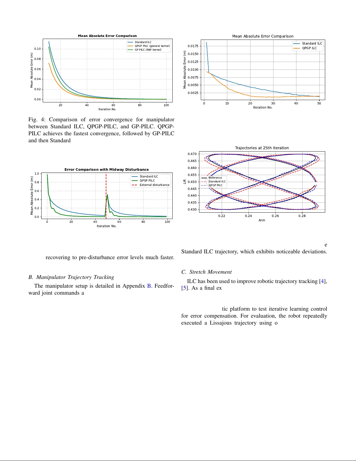
1 Quasi-Periodic Gaussian Process Predicti v e Iterati ve Learning Control Unnati Nigam, Radhendushka Sri vasta va, F aezeh Marzbanrad, Michael Burke Abstract —Repetitive motion tasks are common in robotics, but performance can degrade over time due to envir onmental changes and robot wear and tear . Iterative learning contr ol (ILC) improv es performance by using information from pr e- vious iterations to compensate for expected errors in futur e iterations. This work incorporates the use of Quasi-P eriodic Gaussian Processes (QPGPs) into a predictive ILC framework to model and forecast disturbances and drift across iterations. Using a recent structural equation formulation of QPGPs, the proposed approach enables efficient inference with complexity O ( p 3 ) instead of O ( i 2 p 3 ) , where p denotes the number of points within an iteration and i represents the total number of iterations, specially for larger i . This formulation also enables parameter estimation without loss of information, making continual GP learning computationally feasible within the control loop. By predicting next-iteration error profiles rather than relying only on past errors, the controller achieves faster con vergence and maintains this under time-varying disturbances. W e benchmark the method against both standard ILC and con ventional Gaussian Process (GP)-based predicti ve ILC on three tasks, autonomous vehicle trajectory tracking, a thr ee-link r obotic manipulator , and a real-world Stretch robot experiment. Across all cases, the proposed approach conver ges faster and remains robust under injected and natural disturbances while reducing computational cost. This highlights its practicality across a range of repetitive dynamical systems. Index T erms —Model Lear ning f or Control, Probability and Statistical Methods, Machine Learning for Robot Control. I . I N T R O D U C T I O N ILC is a powerful technique for improving the performance of systems executing repetitiv e tasks [ 1 ]. By leveraging infor- mation from previous iterations, ILC aims to reduce tracking errors ov er successive repetitions, making it particularly suit- able for robotic manipulators, autonomous vehicles, and other cyclic dynamical systems [ 2 ], [ 3 ]. ILC has been widely used to improv e robotic trajectory tracking and motion control [ 4 ]–[ 6 ], as well as in autonomous driving applications [ 7 ] and indus- trial manipulators [ 8 ]. Ho wev er, standard ILC approaches only update control inputs reactiv ely using past errors, despite the fact that error patterns often repeat or e volv e predictably across iterations. This may lead to slow conv ergence, especially under disturbances or when errors exhibit quasi-periodic behaviour . While Quasi-Periodic Gaussian Processes (QPGP) have re- cently been proposed for ef ficient modeling of pseudo-periodic signals, they hav e not been integrated into iterativ e learning control in a way that supports continual, iteration-by-iteration learning with bounded computation. This work shows how a Unnati Nigam is a Ph.D. student at IITB-Monash Research Academy , IIT Bombay , Mumbai, India. Radhendushka Srivasta va is with the Department of Mathematics, IIT Bombay , Mumbai, India. Faezeh Marzbanrad and Michael Burke are with the Department of Electrical and Computer Systems Engineering, Monash Univ ersity , Clayton, Melbourne, Australia. 0 200 400 600 800 1000 Time step for all iterations 0.0 0.2 0.4 0.6 0.8 Signed Lateral Error (m) Errors across iterations (Standard ILC vs. QPGP -PILC) Standar d ILC er r ors QPGP -PILC er r or Fig. 1: Our key insight is that errors in iterativ e learning con- trol e volv e in a quasi-periodic manner . Incorporating predictive modeling exploiting this structure this into ILC (QPGP-PILC) results in noticeably reduced error magnitude and improved con ver gence behaviour over standard ILC. structural equation form of QPGPs can be embedded directly into predictiv e ILC, enabling next-iteration error prediction using only the most recent trial, while remaining conditioned on all past data. W e demonstrate the effecti veness of the proposed QPGP- based predictiv e ILC through three case studies: autonomous vehicle trajectory tracking, a 3-link planar manipulator follow- ing a circular trajectory , and a real-world Hello Stretch robot ex ecuting a Lissajous curve tracking task. These scenarios rep- resent increasingly complex dynamical settings, ranging from simulation to hardware implementation. Across all scenarios, the QPGP-based approach consistently outperforms standard ILC and competing GP-based predictive ILC methods, both under nominal conditions and in the presence of external disturbances. The core contributions of our work are: • Showing that iterative learning control results in a quasi- periodic dynamical system (see Fig. 1 ). • A computationally tractable QPGP-based predictiv e iter- ativ e control method that enables continual learning and ongoing, rapid adaptation to changing en vironments. • A contraction result outlining controller design require- ments to ensure mean error conv ergence when using QPGP predictive iterati ve learning control. I I . B A C K G R O U N D A. Iterative Learning Control (ILC) Consider a system performing a repetitive task ov er a discrete time interval t ∈ { 1 , 2 , . . . , p } . Let u i denote a control vector of dimension mp , and y i a system output vector of dimension np , respectively . Here, m denotes the control input dimension at each timestep, and n the system output dimension at each timestep. These vectors are formed 2 by stacking all p control inputs for each of the k control input dimensions, k = 1 , . . . , m , and all p system outputs for each of the j system output dimensions, j = 1 , . . . , n , into a lifted form. i corresponds to the i th iteration of this repetitiv e task. The discrete-time closed-loop dynamics of the system over iterations (or trials) can be modeled as follows. y i = g ( u i ) + z i , for all i ≥ 1 , (1) where g : R mp → R np is assumed to be continuously differentiable, and is often unknown. Here, z i models the disturbances in these dynamics, a zero mean Gaussian process. Let the tracking error at iteration i be defined as: e i = y d − y i , for all i ≥ 1 . (2) ILC seeks to update the control input for the next iteration to reduce this error . A standard ILC update is giv en by: u i +1 = u i + L i e i , ∀ i ≥ 1 . (3) where L i is the learning gain matrix of dimension mp × np that determines the influence of the previous iteration’ s error e i on the updated input. From ( 1 ) and ( 3 ), using T aylor’ s linearization on g , we have, e i +1 = y d − y i +1 = y d − [ g ( u i ) + G i L i e i + z i +1 ] = ( I np − G i L i ) e i + ( z i − z i +1 ) (4) where G i = ∂ g ∂ u      u = u i . (5) A ke y insight motiv ating this work is that ILC generates quasi-periodic error signals, as sho wn in ( 4 ). Across each iteration, the error is a perturbed version of the previous error . W e demonstrate this graphically in an autonomous racecar path-following task, where steering is the control input and the goal is to minimize tracking error to a fix ed reference across iterations. As sho wn in Fig. 1 , this produces quasi- periodic tracking errors across iterations that can be exploited for prediction. B. Pr edictive ILC Despite its ef fectiveness, standard ILC updates control in- puts reactively using only past tracking errors, which can slow con vergence when error patterns repeat or ev olve pre- dictably [ 1 ]. Predictive ILC (PILC) extends standard ILC by using a model to forecast future errors [ 9 ], [ 10 ]. Instead of relying only on past errors, the controller uses predicted errors for the upcoming iteration, ˆ e i +1 , to proacti vely refine the input [ 11 ]. This explicit compensation accelerates conv ergence and improves tracking, especially when error patterns repeat or have temporal structure [ 11 ]. The predictiv e ILC update, similar to ( 3 ), is given by u i +1 = u i + L i e i + K i ˆ e i +1 , (6) with K i is a predictiv e learning matrix of dimension mp × np and ˆ e i +1 the predicted output error for the ( i + 1) st iteration. Predictiv e ILC often uses linear models [ 12 ] from system identification for simplicity and tractability , while nonlinear approximators like neural networks [ 13 ] handle complex dy- namics. Gaussian Processes (GPs) with RBF kernels [ 14 ] lev erage their probabilistic nature to capture structured er- ror patterns and quantify uncertainty , enabling reliable error forecasts, rapid con vergence, and improved robustness across iterations. Howe ver , GP models face challenges in online or continual learning because the computational cost of parameter estimation and prediction grows cubically with dataset size for standard GP inference (although this can be reduced for T oeplitz matrices [ 15 ]). T o maintain tractability , strategies like data sub-sampling to inducing points [ 16 ]–[ 18 ], using basis vectors [ 19 ], or discarding past observations are employed. Howe ver , these approaches can reduce information and com- promise predictive accuracy . I I I . M E T H O D O L O G Y Having shown the inherent quasi-periodicity in ILC, we propose to employ a recently proposed Quasi-Periodic Gaus- sian Process (QPGP [ 20 ], [ 21 ]) to forecast the next-iteration error trajectory in a predictive ILC framework. T o the best of our knowledge, this is the first predictive ILC framework that exploits quasi-periodic structure across iterations. The framew ork admits mean and covariance contraction results, and scales independently of the number of past iterations. A. Quasi-P eriodic Gaussian Processes (QPGP) A Gaussian process is referred to as QPGP if its sample paths exhibit a quasi-periodic pattern. The covariance structure of a QPGP captures both within-period and between-period variation. [ 22 ] models within-period correlations with a pe- riodic kernel and between-period correlations with geometric decay . Howe ver , the prediction of this QPGP is computation- ally expensi ve (see [ 21 ]). One approach to reduce complexity for GP kernels is to vie w these from a state-space or dynamical systems perspective [ 23 ]. Along these lines, [ 21 ] proposed a family of dynamical- system-based QPGP that permits general periodic kernels to model the within-period correlation of the QPGP . [ 21 ] also provides a computationally efficient parameter estimation and prediction of the QPGP . In this framew ork, the within period blocks of a vector x i , for i ≥ 1 satisfy x i +1 = ω x i + ϵ i +1 (7) where ω ∈ ( − 1 , 1) captures inter-iteration correlation, and ϵ i are i.i.d. zero-mean Gaussian vectors. Stacking [ x ⊤ 1 x ⊤ 2 . . . ] ⊤ exhibits quasi-periodic behavior . This formulation allows pre- diction of the next iteration using only the most recent error , enabling efficient online updates [ 21 ]. W e propose to model the evolving error dynamics under the standard ILC law in ( 4 ) independently for each of the j = 1 , 2 , . . . , n output dimensions using ( 7 ), assuming the I np − G i L i term in ( 4 ) is approximately diagonal: e i +1 ≈ (Ω ⊗ I p ) e i + ε i +1 (8) with ε i +1 ∼ N ( 0 , blkdiag { K 1 , . . . , K n } ) . This is reasonable in robotic systems with weak cross-coupling or after suitable coordinate transformation or feedback diagonalization by the 3 inner loop controller , and it simplifies learning gain design while maintaining computational efficienc y (Sections III-B , III-D ). Although the disturbance in ( 4 ) is temporally corre- lated, the dependence typically lasts only one iteration. W e model the noise using a zero-mean i.i.d. Gaussian vector with cov ariance K j to pro vide a simpler representation that captures the dominant and unmodeled residual noise characteristics without introducing unnecessary complexity . B. Incorporating QPGP in ILC: Pr ediction For j = 1 , 2 , . . . , n , the error in j th output dimension at iteration i corresponds to the p -dimensional subvector of e i from the index ( j − 1) p + 1 to j p and is denoted as follows. e i,j = e i [( j − 1) p + 1 : j p ] = [ e i,j (1) , e i,j (2) , . . . , e i,j ( p )] ⊤ . A prediction of each of these, i.e. ˆ e i,j is required in ( 6 ). Depending on the compute requirements of the control prob- lem, we can exploit two prediction strategies, gi ven by [ 21 ]. Element-wise pr ediction predicts each element ˆ e i +1 ,j ( t ) se- quentially for all t = 1 , . . . , p , while Block pr ediction predicts the entire error e i +1 ,j simultaneously . Element-Wise Prediction: In the element-wise prediction approach, gi ven by [ 21 ], each element e i +1 ( t ) can be predicted sequentially ˆ e i +1 ,j ( t ) = ω j e i,j ( t ) + K j ;1 ,t − 1 K − 1 j ; t − 1  e ( t − 1) i +1 ,j − ω j e ( t − 1) i,j  (9) The vector K j ;1 ,t − 1 contains the first t − 1 elements of the first row of K j , while K j ; t − 1 represents the submatrix formed by the first t − 1 rows and columns of K j . The terms e ( t − 1) i +1 ,j and e ( t − 1) i,j − 1 correspond to the first t − 1 ele- ments of e i +1 ,j and e i,j respectiv ely . This expression provides the best predictor of e i +1 ,j ( t ) as the conditional mean of e i +1 ,j ( t ) given the pre vious observations in the same iteration e i +1 ,j ( t − 1) , . . . , e i +1 ,j (1) and the observ ations from previous iterations, e i,j , e i − 1 ,j , . . . , e 1 ,j . For t = 1 , the second term vanishes and ˆ e i +1 ,j (1) = ω j e i,j (1) . Block Prediction: In the block prediction approach, the prediction is obtained using ˆ e i +1 ,j = ω j e i,j . (10) This prediction represents the best predictor of e i +1 ,j , deri ved as the conditional mean of e i +1 ,j giv en the observations in the pre vious iterations, e i,j , e i − 1 ,j , . . . , e 1 ,j . This is computa- tionally efficient, but does not exploit the cov ariance structure within an iteration, providing a simple linear prediction. Notably , these formulations depend only on the immedi- ately preceding error block e i,j , making them computationally lightweight and tractable for online learning settings like ILC. Specifically , the computational complexity of ( 10 ) is O ( p ) , while that of ( 9 ) is O ( p 3 ) , where p denotes the number of points in the iteration. In contrast, a con ventional GP approach requires O ( i 2 p 3 ) computations at iteration i , which becomes increasingly costly for iterativ e, online applications. In general, element-wise prediction should be preferred for accuracy , unless the length of each trial prohibits computation at the required control frequency . It is worth noting that an alternative computationally ef- ficient approach to GP modeling is the use of sparse GPs [ 17 ], which approximate a full GP using M inducing points. For prediction, this reduces the computational complexity to O ( pM 2 ) . When M > p , both element-wise and block QPGP-based prediction offer reduced computation. Howe ver , ev en with M < p , sparse GPs may be computationally more expensi ve than a QPGP , as selecting an optimal set of inducing points can itself be challenging; methods such as greedy selection [ 24 ], variational optimization [ 25 ], or k- means based initialization are commonly used, and cross- validation over multiple choices of M may be required, which further increases computational cost. While sparse GPs in volv e information loss that QPGPs a void, they could nonetheless be used to model the within-block cov ariance in the block QPGP framew ork, offering additional flexibility and efficiency . As shown in our experimental results, element-wise QPGPs gen- erally provide higher accuracy , and block-wise QPGPs achieve better con ver gence with significantly lower computation time. C. Incorporating QPGP in ILC: Stability In predicti ve ILC, the goal is to anticipate the ne xt iteration’ s tracking error rather than relying only on past errors. T o achiev e this, we use the QPGP to model (Section III-A ) and predict (Section III-B ) the ev olution of error trajectories across iterations. T o characterize the behaviour of the proposed QPGP-based predictiv e ILC, the follo wing theorem presents stability results for oracle prediction models. Theorem 1. Consider the nonlinear discr ete-time system given in ( 1 ) and define the tracking error as in ( 2 ) . Assume g is locally linearizable ar ound the curr ent input with its J acobian given in ( 5 ) . Then, for the two control strate gies, 1) Element-wise pr ediction: The trac king err or e i ∈ R np evolves as e ( t ) i +1 = B i e ( t ) i + ( z ( t ) i − z ( t ) i +1 ) , ∀ t = 1 , . . . , p. (11) wher e, B i = I nt − G ( t ) i L ( t ) i − G ( t ) i K ( t ) i M ( t ) i , wher e M ( t ) i = L n j =1 M ( t ) i,j , M (1) i,j = ω j and for t = 2 , . . . , p , M ( t ) i,j = " M ( t − 1) i,j 0 K j ;1 ,t − 1 K − 1 j ; t − 1  M ( t − 1) i,j − ω j I t − 1  ω j # . and G ( t ) i , L ( t ) i and K ( t ) i ar e sub-matrices formed by the first t columns of matrices G i , L i and K i r espectively . Further , if ther e exists a constant γ E ∈ [0 , 1) and C > 0 , such that sup i || B i || 2 ≤ γ E and sup j || K j || 2 < C / 2 then for all t = 1 , . . . , p , lim i →∞ E  e ( t ) i  = 0 , and lim i →∞       Cov  e ( t ) i        2 < C . (12) 2) Block prediction: The tracking err or e i ∈ R np , for the i th iteration, evolves as e i +1 = A i e i + ( z i − z i +1 ) . (13) wher e, A i = I np − G i L i − G i K i (Ω ⊗ I p ) and wher e Ω = diag { ω 1 , . . . , ω n } . Further , if ther e exists a constant 4 γ B ∈ [0 , 1) and C > 0 , such that sup i || A i || 2 ≤ γ B and max 1 ≤ j ≤ n || K j || 2 < C / 2 then lim i →∞ E ( e i ) = 0 , and lim i →∞ || Cov ( e i ) || 2 < C (14) Using ( 1 ) and ( 6 ), and using the T aylor’ s linearization on g , we have, e i +1 = ( I np − G i L i ) e i − G i K i ˆ e i +1 + ( z i − z i +1 ) (15) For 1) Element-wise prediction: W e have, from ( 9 ), ˆ e ( t ) i +1 = M ( t ) i e ( t ) i Then, for t = 1 , 2 , . . . , p , e ( t ) i +1 =  I nt − G ( t ) i L ( t ) i − G ( t ) i K ( t ) i M ( t ) i  e ( t ) i +  z ( t ) i − z ( t ) i +1  Then, as E  z ( t ) i  = 0 , for all i ≥ 1 , then E  e ( t )  = B ( t ) i E  e ( t ) i  (16) If there exists γ E ∈ [0 , 1) such that sup i     B ( t ) i     2 ≤ γ E then E  e ( t ) i +1  ≤ γ i B E  e ( t ) i  → 0 (17) Let P ( t ) i = Cov  e ( t ) i  . Then, P ( t ) i +1 = B ( t ) i P ( t ) i B ( t ) i ⊤ + 2 n M j =1 K j ; t T aking the norm on both sides, we hav e     P ( t ) i +1     2 ≤ γ 2 i E     P i     2 + max 1 ≤ j ≤ n     K j ; t     2 (18) As γ E ∈ [0 , 1) and || K j ; t || 2 < C / 2 , for all j = 1 , . . . , n , lim i →∞       Cov  e ( t ) i        2 < C , for all t = 1 , 2 , . . . , p. (19) For 1) Block prediction: we have, ˆ e i +1 = (Ω ⊗ I p ) e i . Then e i +1 = ( I np − G i L i − G i K i (Ω ⊗ I p )) e i + ( z i − z i +1 ) (20) Then, as E ( z i ) = 0 , for all i ≥ 1 , then E ( e i +1 ) = A i E ( e i ) (21) If there exists γ B ∈ [0 , 1) such that sup i || A i || 2 ≤ γ B then E ( e i +1 ) ≤ γ i B E ( e i ) → 0 (22) Let P i = Cov ( e i ) . Then, P i +1 = A i P i A ⊤ i + 2 n M j =1 K j T aking the norm on both sides, we hav e || P i +1 || 2 ≤ γ 2 i B || P i || 2 + max 1 ≤ j ≤ n || K j || 2 (23) As γ B ∈ [0 , 1) and || K j || 2 < C / 2 , for all j = 1 , . . . , n , lim i →∞ || Cov ( e i ) || 2 < C (24) The theorem first establishes stability at the lev el of the mean behavior of the tracking error . When the lifted iteration dynamics are contracti ve, the expected tracking error decreases from one iteration to the next, demonstrating that the controller consistently corrects past mistakes and refines the control input. As a result, the system learns the desired trajectory in an av erage sense despite the presence of modeling inaccuracies and stochastic perturbations. This guarantees that the learning mechanism is not merely reactive but progressiv ely improves performance over repeated trials. At the second-moment level, the theorem ensures that the uncertainty associated with the tracking error does not grow unbounded. By requiring a uniform spectral bound on the kernel cov ariance matrices, the predictive component is prevented from amplifying stochastic disturbances as the iterations ev olve. Consequently , the error covariance remains bounded, which implies mean-square stability of the learning process and ensures that variability around the desired trajec- tory stays controlled rather than escalating over time. As is standard in ILC, practical implementation the contrac- tion condition and cov ariance bounds translate directly into criteria for selecting the learning gain L i and the predictiv e gain K i for i th iteration. When G i is known, gains can be tuned relativ ely aggressiv ely so that the induced iteration operator remains contractive while the associated cov ariance operators are uniformly bounded. If this is not known, more cautious gain choices can be made (eg. by decaying the learning rate over time). D. Incorporating QPGP in ILC: P arameter Estimation W e adopt the computationally efficient method of obtaining consistent estimators of the parameters ω j and K j from [ 21 ]. This uses a two-stage algorithm, for e very output dimension j = 1 , . . . , n . In Stage I, an iterative, alternating minimization is applied to a reduced likelihood function, which excludes the marginal contribution of the initial error block e 1 ,j . This iterativ ely estimates ω j and an unconstrained cov ariance matrix, ˜ K j . In Stage II, the estimated covariance matrix ˜ K j is projected onto the set of v alid periodic cov ariance kernels by averaging along the diagonals and ensuring positive definiteness through spectral truncation [ 26 ]. The resulting estimates, ˆ ω j and ˆ K j are consistent, con ver ging in probability to the true parameters as the number of iterations increase. Further , if the cov ariance function is from a known parametric family , the hyperparameters of the cov ariance function can be calculated using ( ˆ σ 2 j , ˆ θ j ) = arg min ( σ 2 , θ ) ∈ (0 , ∞ ) × Θ ∥ ˜ K j − K ( σ 2 , θ ) ∥ F . (25) In the absence of prior structural knowledge of the parametric family , the estimate ˆ K j is retained directly and treated as a general kernel obtained purely through a data-driv en process. In the predictive ILC setting, the two-stage estimation pro- cedure naturally integrates into the iterative update framew ork. After iteration i , the new tracking errors e i,j are incorporated into the training dataset, for all j = 1 , 2 , . . . , n . The aggregated training data up to iteration i is thus given by [ e ⊤ 1 ,j , . . . , e ⊤ i,j ] ⊤ for output index j . Using this updated dataset, the parameters 5 T ABLE I: T otal Computation time (in secs.) for 100 iterations for Standard ILC, GP-PILC, Sparse GP-PILC and QPGP-PILC (block and element-wise). Appr oach Standard QPGP QPGP Sparse GP (block) (element) GP Time (secs.) 0.23 18.74 19.31 19.67 649.23 are re-estimated via the two-stage procedure to obtain ˆ ω ( i ) j and ˆ K ( i ) j . W e initialize the estimation process with parameters from the previous trial. These updated estimates are then employed for prediction after each iteration. Since prediction is implemented using plug-in estimates ˆ ω ( i ) j and ˆ K ( i ) j , finite-sample estimation error can introduce predictor mismatch relativ e to the ideal QPGP conditional mean. Accordingly , when tuning L i and K i in practice, we recommend maintaining a nontri vial contraction margin in Theorem 2 (e.g., selecting gains so that ∥ A i ∥ 2 or ∥ B i ∥ 2 are comfortably below 1 ) to ensure robust stability under this mismatch. I V . E X P E R I M E N T S W e compare the performance of the QPGP-based predicti ve ILC (QPGP-PILC) framework with Standard ILC and GP- based predictive ILC (GP-PILC) using three scenarios. A vehicle following a predefined path, with QPGP-PILC anticipating recurring steering errors and correcting these via block- and element-wise predictions using ( 10 ) and ( 9 ). A three-link robotic manipulator tracking a repetiti ve trajectory , where QPGP-PILC improv es tracking accuracy and con ver gence. An external disturbance midway ev aluates the method’ s robustness against unexpected perturbations. A Stretch Robot tracking problem, which shows QPGP- PILC ef fectiv ely handles uncertainties and actuator noise while achieving faster con ver gence and lower tracking errors. For each case, we analyze tracking error , conv ergence speed, and computational efficiency , demonstrating the clear advantages of QPGPs for predictive error correction in ILC. A. V ehicle T rajectory T r acking Using the experimental procedure in Appendix A , we ev aluate con vergence and tracking performance of Standard ILC, GP-PILC, and QPGP-PILC controllers. The feedforward steering input ( δ ff k ) is updated iterati vely according to each ILC variant ( 3 ) or ( 6 ), allowing assessment of predicti ve modeling effects on error reduction and trajectory accuracy . Standard ILC updates the input solely using the pre vious iteration’ s tracking error ( 3 ). T wo predictiv e ILC variants are considered ( 6 ). GP-PILC employs a Gaussian Process with an RBF kernel to model the expected error . Although it con ver ges faster than Standard ILC, it requires the complete error history , resulting in high computational cost (T able I ). A Sparse GP with M = 100 optimized inducing points reduces computation, achieving runtimes closer to QPGP-PILC, but its prediction accuracy remains lower . QPGP-PILC lev erages the quasi-periodic structure of the error signal, capturing recurring patterns while using only the 20 40 60 80 100 Iteration No . 0.04 0.06 0.08 0.10 0.12 0.14 Mean Abs. Er r or (m) Mean Absolute Error Comparison Standar d ILC QPGP -PILC (general k er nel, Block pr ediction) QPGP -PILC (general k er nel, Element pr ediction) GP -PILC (RBF k er nel) Sparse GP (RBF k er nel) Fig. 2: Comparison of error con vergence for vehicle trajectory tracking for Standard ILC, GP-PILC, Sparse GP-PILC, and QPGP-PILC (block and element-wise). Element-wise QPGP- PILC conv erges fastest, followed by block-based QPGP-PILC. GP-PILC shows similar con vergence, while Sparse GP-PILC con ver ges slightly slower . QPGP-PILC consistently achie ves the most accurate tracking. 3 2 1 0 1 2 3 X P osition (m) 3 2 1 0 1 2 3 Y P osition (m) T rajectories of V ehicle R efer ence T rack Iteration 50 of Standar d ILC Iteration 50 of QPGP PILC Fig. 3: Comparison of vehicle trajectories at the 50th iteration under Standard ILC and QPGP-PILC controllers. The QPGP- PILC trajectory closely follows the reference, whereas the Standard ILC trajectory shows visible deviations. most recent error block. Both block- and element-wise predic- tors are ev aluated, consistently achieving higher accuracy than full or sparse GP ILC. Simulation results (Fig. 2 ) show GP- and QPGP-based methods con verge faster than Standard ILC, with the element-wise QPGP predictor con verging faster than the block-based variant at moderate additional cost (T able I ). Unlike GP-based methods, QPGP-PILC avoids storing full error histories, greatly reducing computation. At the 50th iteration (Fig. 3 ), QPGP-PILC trajectories align closely with the reference path, whereas Standard ILC shows visible deviations, demonstrating QPGP-PILC’ s ability to exploit quasi-periodic patterns for faster con ver gence and improv ed tracking accuracy . 6 20 40 60 80 100 Iteration No . 0.00 0.02 0.04 0.06 0.08 0.10 Mean Absolute Er r or (m) Mean Absolute Error Comparison Standar d ILC QPGP PILC (general k er nel) GP PILC (RBF k er nel) Fig. 4: Comparison of error conv ergence for manipulator between Standard ILC, QPGP-PILC, and GP-PILC. QPGP- PILC achie ves the fastest con ver gence, followed by GP-PILC and then Standard ILC. In addition to its superior conv ergence rate, QPGP-PILC is computationally more efficient, as it requires only the most recent iteration’ s errors for predictions. 0 20 40 60 80 100 Iteration No . 0.0 0.2 0.4 0.6 0.8 1.0 Mean Absolute Er r or (m) Error Comparison with Midwa y Disturbance Standar d ILC QPGP PILC Exter nal disturbance Fig. 5: Response of the manipulator to a mid-iteration dis- turbance under Standard ILC and QPGP-PILC. Standard ILC reacts slowly , while QPGP-PILC anticipates and corrects de vi- ations, recovering to pre-disturbance error lev els much faster . B. Manipulator T rajectory T rac king The manipulator setup is detailed in Appendix B . Feedfor- ward joint commands are updated through the Jacobian using ( 3 ) for Standard ILC and ( 6 ) for predictive ILC. Standard ILC updates joint angles solely using the previous iteration’ s errors, reducing errors slowly . Predictiv e ILC meth- ods, including GP- and QPGP-PILC, model error dynamics to anticipate deviations. GP-PILC uses the full history of joint errors, whereas QPGP-PILC lev erages quasi-periodic patterns and requires only the most recent block for prediction. Simulations show that both GP- and QPGP-PILC con verge faster than Standard ILC (Fig 4 ), with QPGP-PILC achieving the fastest error reduction and closely tracking the reference trajectory . This highlights the benefit of predicti ve probabilistic modeling in multi-joint learning using QPGPs. A mid-iteration disturbance was introduced to test robust- ness. Standard ILC reacts slo wly , taking sev eral iterations to recov er . QPGP-PILC, using learned quasi-periodic error patterns, quickly corrects the perturbation and restores pre- disturbance accuracy , demonstrating robust and reliable tra- jectory tracking. (Fig. 5 ). This suggests that the diagonal approximation in ( 8 ) remains effecti ve ev en in moderately coupled robotic systems. 0 10 20 30 40 50 Iteration No . 0.0025 0.0050 0.0075 0.0100 0.0125 0.0150 0.0175 Mean Absolute Er r or (m) Mean Absolute Er r or Comparison Standar d ILC QPGP ILC Fig. 6: Conv ergence of tracking error for Hello Robot Stretch 3 over iterations for standard ILC and QPGP-based PILC. The QPGP-PILC achieves faster con vergence than Standard ILC. 0.22 0.24 0.26 0.28 Ar m 0.430 0.435 0.440 0.445 0.450 0.455 0.460 0.465 0.470 Lif t T rajectories at 25th iteration R efer ence Standar d ILC QPGP PILC Fig. 7: Tracking performance of Hello Robot Stretch 3 at 25th iteration under Standard ILC and QPGP-PILC controllers. The QPGP trajector is closer to the reference path compared to the Standard ILC trajectory , which exhibits noticeable deviations. C. Str etch Movement ILC has been used to improv e robotic trajectory tracking [ 4 ], [ 5 ]. As a final experiment, we demonstrate the use of QPGPs on a real robot, the Hello Robot Stretch 3. The Stretch robot, being a servo- and cable-dri ven arm with inherent backlash, serves as a realistic platform to test iterativ e learning control for error compensation. For ev aluation, the robot repeatedly ex ecuted a Lissajous trajectory using only the lift and arm joints (Appendix C ). Standard ILC updates inputs reactiv ely from previous errors, while QPGP-PILC anticipates deviations by modeling the quasi-periodic error structure. QPGP-PILC conv erges faster than Standard ILC, effecti vely capturing the repeated Lissajous motion and reducing errors more quickly and stably . Its trajectory remains closer to the reference path, demonstrating improved tracking accuracy and confirming its practical advantages for learning-based control. V . C O N C L U S I O N W e proposed a QPGP-based predictive iterativ e learning control (PILC) framework to improve trajectory tracking in re- peated robotic tasks. Analysis of standard ILC errors rev ealed quasi-periodic patterns not explicitly captured by con ventional methods. By integrating quasi-periodic Gaussian processes, the 7 framew ork estimates system parameters and forecasts future trajectory errors, enabling proactiv e control adjustments. QPGP-PILC is well-suited for non-stationary continual learning, handling slowly varying dynamics or en vironmental changes efficiently using only the previous iteration’ s errors. The proposed approach showed faster con vergence and im- prov ed tracking error across multiple en vironments. Overall, QPGP-PILC offers a powerful approach for enhancing per- formance in repetitive robotic and industrial tasks requiring continual learning with fixed memory and fixed computational complexity . R E F E R E N C E S [1] D. Bristow , M. Tharayil, and A. Alleyne, “ A survey of iterati ve learning control, ” IEEE Control Systems Magazine , vol. 26, no. 3, pp. 96–114, 2006. [2] H.-S. Ahn, Y . Chen, and K. L. Moore, “Iterative learning control: Brief survey and categorization, ” IEEE T ransactions on Systems, Man, and Cybernetics, P art C (Applications and Revie ws) , vol. 37, no. 6, pp. 1099– 1121, 2007. [3] H.-S. Ahn, K. L. Moore, and Y . Chen, Iterative Learning Control: Robustness and Monotonic Con verg ence for Interval Systems . Springer Publishing Company , Incorporated, 1st ed., 2007. [4] C. Nguyen, L. Bao, and Q. Nguyen, “Mastering agile jumping skills from simple practices with iterative learning control, ” in 2025 IEEE International Conference on Robotics and Automation (ICRA) , 2025. [5] K. Qian, Z. Li, Z. Zhang, G. Li, and S. Q. Xie, “Data-driv en adaptive iterativ e learning control of a compliant rehabilitation robot for repetitiv e ankle training, ” IEEE Robotics and Automation Letters , vol. 8, 2023. [6] M. Arif, T . Ishihara, and H. Inooka, “Experience-based iterative learning controllers for robotic systems, ” J. Intell. Robotics Syst. , vol. 35, p. 381–396, Dec. 2002. [7] Y . Q. Chen and K. L. Moore, “ A practical iterativ e learning path- following control of an omni-directional vehicle, ” Asian Journal of Contr ol , vol. 4, no. 1, pp. 90–98, 2002. [8] J.-Y . Choi, J. Uh, and J. S. Lee, “Iterative learning control of robot manipulator with i-type parameter estimator , ” in Pr oceedings of the 2001 American Control Conference , vol. 1, pp. 646–651 v ol.1, 2001. [9] M. Rzewuski, E. Rogers, and D. Owens, “Prediction in iterative learning control schemes versus learning along the trials, ” IF AC Pr oceedings V olumes , vol. 35, no. 1, pp. 7–12, 2002. 15th IF A C W orld Congress. [10] S. N. Huang and S. Y . Lim, “Predictiv e iterativ e learning control, ” Intelligent Automation & Soft Computing , vol. 9, no. 2, pp. 103–112, 2003. [11] D. H. Owens, “The benefits of prediction in learning control algorithms, ” in T wo-Day W orkshop on Model Predictive Contr ol: T echnology and Applications – Day 1 , (London, U.K.), pp. 3/1–3/3, Institution of Electrical Engineers, Apr . 1999. [12] J. H. Lee, K. S. Lee, and W . C. Kim, “Model-based iterative learning control with a quadratic criterion for time-varying linear systems, ” Automatica , vol. 36, no. 5, pp. 641–657, 2000. [13] K. Patan and M. Patan, “Neural-network-based iterativ e learning control of nonlinear systems, ” ISA T ransactions , vol. 98, pp. 445–453, 2020. [14] A. Buelta, A. Oliv ares, E. Staffetti, W . Aftab, and L. Mihaylova, “ A gaussian process iterative learning control for aircraft trajectory tracking, ” IEEE Tr ansactions on Aerospace and Electr onic Systems , vol. 57, no. 6, pp. 3962–3973, 2021. [15] M. H. Hayes, Statistical Digital Signal Processing and Modeling . USA: John Wiley & Sons, Inc., 1st ed., 1996. [16] N. Lawrence, M. Seeger, and R. Herbrich, “Fast sparse gaussian process methods: The informativ e vector machine, ” in Advances in Neural Information Processing Systems , vol. 15, pp. 625–632, MIT Press, 2002. [17] E. Snelson and Z. Ghahramani, “Sparse gaussian processes using pseudo-inputs, ” in Advances in Neural Information Pr ocessing Systems , vol. 18, pp. 1257–1264, MIT Press, 2005. [18] C. K. I. W illiams and M. Seeger , “Using the nystr ¨ om method to speed up kernel machines, ” in Advances in Neural Information Processing Systems , vol. 13, pp. 682–688, MIT Press, 2000. [19] M. F . Huber , “Recursive gaussian process: On-line regression and learning, ” P attern Recognition Letters , vol. 45, pp. 85–91, 2014. [20] U. Nigam, R. Sriv astav a, M. Burke, and F . Marzbanrad, “ A dynamical equation approach for quasi-periodic gaussian processes, ” in ICASSP 2025 - 2025 IEEE International Conference on Acoustics, Speech and Signal Processing (ICASSP) , pp. 1–5, 2025. [21] U. Nigam, R. Srivasta va, F . Marzbanrad, and M. Burke, “ A structural equation formulation for general quasi-periodic gaussian processes, ” arXiv:2511.01151 , 2025. [22] Y . Li, Y . Zhang, Q. Xiao, and J. Wu, “Quasi-periodic gaussian process modeling of pseudo-periodic signals, ” IEEE T ransactions on Signal Pr ocessing , vol. 71, pp. 3548–3561, 2023. [23] A. Solin and S. S ¨ arkk ¨ a, “Explicit Link Between Periodic Covariance Functions and State Space Models, ” in Proceedings of the Seventeenth International Conference on Artificial Intelligence and Statistics , vol. 33 of Proceedings of Machine Learning Research , PMLR, 2014. [24] A. J. Smola and P . L. Bartlett, “Sparse greedy gaussian process regres- sion, ” in Advances in Neural Information Processing Systems , vol. 13, pp. 619–625, MIT Press, 2000. [25] M. Titsias, “V ariational learning of inducing variables in sparse gaussian processes, ” in Pr oceedings of the T welfth International Conference on Artificial Intelligence and Statistics , vol. 5 of Proceedings of Machine Learning Research , pp. 567–574, PMLR, 16–18 Apr 2009. [26] P . Hall, N. I. Fisher , and B. Hoffmann, “On the nonparametric estimation of cov ariance functions, ” Ann. Statist. , vol. 22, no. 4, pp. 2115–2134, 1994. [27] R. C. Coulter, “Implementation of the pure pursuit path tracking al- gorithm, ” T ech. Rep. CMU-RI-TR-92-01, Carnegie Mellon University , Robotics Institute, 1992. A P P E N D I X The code for all three experiments described in this paper is av ailable at our GitHub repository . 1 A. V ehicle Experimental Setup Reference Raceline Generation: A smooth closed race- track is generated using a polar parameterization with s ∈ [0 , 2 π ] and p uniformly spaced points. R ( s ) = 10 + 2 sin(2 s ) + sin(3 s ) , (26) and the corresponding Cartesian coordinates are x ref ( s ) = R ( s ) cos( s ) , y ref ( s ) = R ( s ) sin( s ) . (27) Discretized points are s j = 2 π j p , j = 1 , . . . , p , and the curve is scaled so the total length equals L d = v , ∆ t, p , where v is vehicle speed and ∆ t is the timestep. V ehicle Dynamics per Lap: For lap i and step k , the vehicle state ( x ( i ) k , y ( i ) k , θ ( i ) k ) evolv es as: x ( i ) k +1 = x ( i ) k + v cos( θ ( i ) k ) ∆ t, (28) y ( i ) k +1 = y ( i ) k + v sin( θ ( i ) k ) ∆ t, (29) θ ( i ) k +1 = θ ( i ) k + v L tan( δ ( i ) k ) ∆ t + d θ , (30) where v = 8 m/s is the constant longitudinal velocity , W = 0 . 5 m is the wheelbase, and d θ = 0 . 04 is a small heading drift. The steering input is δ ( i ) k = g  δ ff , ( i ) k + δ fb , ( i ) k  + b 0 + b 1 k + ε ( i ) k , (31) where g = 0 . 7 is the steering gain, b 0 = 0 . 15 is a constant bias, b 1 = 0 . 01 is the slope of a slowly increasing drift, and ε ( i ) k ∼ N (0 , σ 2 ) , with σ 2 = 0 . 015 , is Gaussian noise. The steering angle is saturated to | δ ( i ) k | ≤ 0 . 5 radians. 1 https://github .com/unnati- nigam/QPGP- PILC 8 Feedback Control: The feedback steering δ fb , ( i ) k is com- puted using a pure pursuit geometric controller [ 27 ]. Let ( x ref ,k +1 , y ref ,k +1 ) be the next reference point: ∆ x k = x ref ,k +1 − x ( i ) k , ∆ y k = y ref ,k +1 − y ( i ) k , (32) ψ k = tan − 1  ∆ y k ∆ x k  , α k = ψ k − θ ( i ) k , (33) δ fb , ( i ) k = tan − 1  2 L sin( α k ) √ ∆ x 2 k +∆ y 2 k  . (34) Lateral Error Computation: The signed lateral deviation of the vehicle from the reference trajectory at step k is e ( i ) k = n ⊤ ⋆ " x ( i ) k y ( i ) k # −  x ref ,⋆ y ref ,⋆  ! , (35) where ⋆ is the index of the nearest reference point and t ⋆ =  x ref ,⋆ +1 − x ref ,⋆ − 1 y ref ,⋆ +1 − y ref ,⋆ − 1       x ref ,⋆ +1 − x ref ,⋆ − 1 y ref ,⋆ +1 − y ref ,⋆ − 1      , n ⋆ =  − t y ,⋆ t x,⋆  . (36) Learning and predictive gains were annealed across itera- tions according to a 1 /i schedule. The diminishing step size enabled large correctiv e updates in the initial laps and progres- siv ely smaller adjustments thereafter, improving robustness to noise and promoting stable tracking error con vergence. B. Manipulator Experimental Setup Reference T rajectory: The manipulator is required to follow a smooth, repetitiv e trajectory in the Cartesian plane. The desired end-effector path is a circular path defined as: x ref ( s ) = 1 . 5 + 0 . 5 cos( s ) , y ref ( s ) = 1 . 0 + 0 . 5 sin( s ) (37) where s ∈ [0 , 2 π ] and the trajectory is sampled at p uniformly- spaced discrete points to generate the reference for simulation. Manipulator: The system is a 3-link planar manipulator oper- ating in the XY -plane. The manipulator has 3 links, l 1 = 1 . 0 m, l 2 = 1 . 0 m, and l 3 = 0 . 5 m. It has three joints with angles θ 1 , θ 2 , θ 3 , measured relativ e to the previous link. The forward kinematics of the manipulator , giving the i-th positions of the 3 joints and the end-effector , are ( x 0 , y 0 ) = (0 , 0) , ( x i , y i ) = i X k =1 l k  cos( P k j =1 θ j ) , sin( P k j =1 θ j )  . (38) The Jacobian matrix, relating joint velocities to end-effector velocities, is given by ( 39 ). J =       − 3 X k =1 l k sin k X s =1 θ s ! − 3 X s =2 l k sin k X s =1 θ s ! − l 3 sin  P 3 s =1 θ s  3 X k =1 l k cos k X s =1 θ s ! 3 X k =2 l k cos i X s =1 θ s ! l 3 cos  P 3 s =1 θ s        (39) In verse Kinematics (IK): In verse kinematics computes the joint angles ( θ 1 , θ 2 , θ 3 ) required to reach a desired end-ef fector position ( x ref , y ref ) . For a planar 3-link arm, exact IK can be complex; here the third joint orientation is ignored ( θ 3 = 0 ). The desired wrist position (excluding the last link) is x e = x ref − l 3 , y e = y ref (40) The first two joint angles are obtained geometrically: D = x 2 e + y 2 e − l 2 1 − l 2 2 2 l 1 l 2 (41) θ 2 = tan − 1 2  p 1 − D 2 , D  (42) θ 1 = tan − 1 ( y e , x e ) − tan − 1  l 2 sin θ 2 , l 1 + l 2 cos θ 2  (43) This provides an approximate initial feedforward joint tra- jectory for the manipulator to follow the desired path. At each iteration i , the manipulator executes the feedforward joint angles with unknown biases. Let s be a vector of p equally spaced points in [0 , 1] , then b 1 ( s t ) = 0 . 2 + 0 . 5 sin(8 π s t ) + ϵ (1) t , ϵ (1) t ∼ N (0 , 0 . 1 2 ) , b 2 ( s t ) = − 0 . 25 + 0 . 1 cos(6 π s t ) + ϵ (2) t , ϵ (2) t ∼ N (0 , 0 . 2 2 ) , b 3 ( s t ) = 0 . 35 + 0 . 5 exp − ( s t − 0 . 04) 2 2(0 . 05) 2 ! + ϵ (3) t , ϵ (3) t ∼ N (0 , 0 . 1 2 ) . are the biases for each joint angle θ actual j = θ ff j + b j ( s ) , j = 1 , 2 , 3 (44) T racking Error: at the i th iteration is computed as the Euclidean norm of the position errors || e i || 2 =      x ref − x ( i ) ee y ref − y ( i ) ee      2 . The learning gain was set to L = 0 . 25 , and the prediction gain to K = 0 . 3 , for all iterations, providing stable and consistent error reduction across iterations. C. Robot Experimental Setup The Hello Robot Stretch 3 was controlled using Python via the official stretch_body API 2 , interacting through the Robot class for high-lev el commands. The true end- effector positions were obtained from the robot’ s onboard joint encoders through the API ( robot.arm.status[’pos’] and robot.lift.status[’pos’] ) at each control step. The control loop executed at approximately 10 Hz( time.sleep(0.1) between commands), resulting in an end-to-end latency of roughly 0.1–0.15 s. The robot followed a smooth trajectory within the workspace limits of the arm and lift joints, as defined in the experiment. Reference T rajectory: For t ∈ [0 , 2 π ) , y ( t ) = 0 . 25 + 0 . 04 sin(3 t + π / 2) , z ( t ) = 0 . 45 + 0 . 02 sin(2 t ) . T racking Error: at the i th iteration is computed as the Euclidean norm of the position errors || e i || 2 =      y ref − y ( i ) ee z ref − z ( i ) ee      2 . The learning gain was set to L = 0 . 05 , and the prediction gain to K = 1 . 5 , for all iterations, providing stable and consistent error reduction across iterations. 2 https://www .hello- robot.com/pages/stretch