Preconditioned Robust Neural Posterior Estimation for Misspecified Simulators

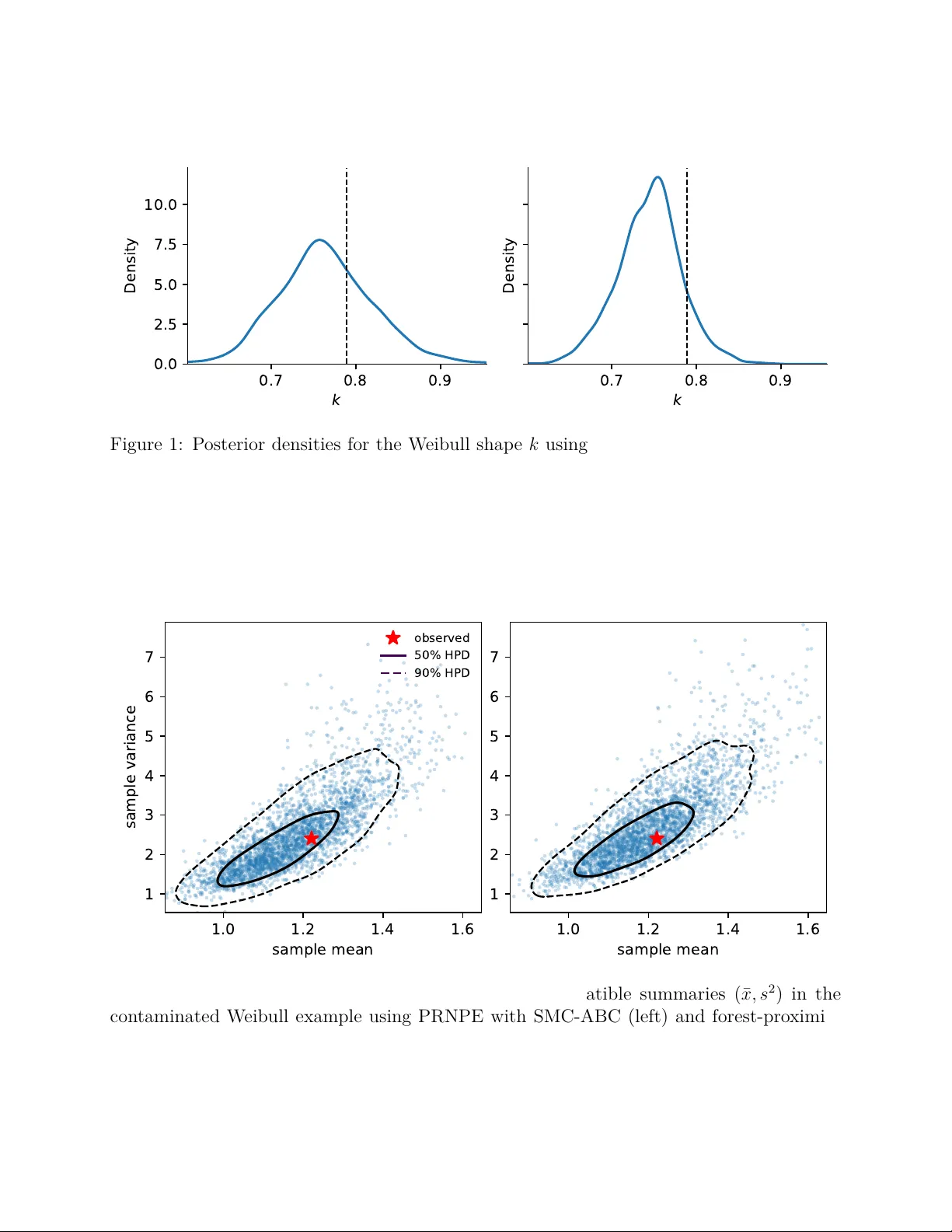
Preconditioned Robust Neural P osterior Estimation for Missp ecified Sim ulators R y an P . Kelly ∗ Sc ho ol of Mathematical Sciences, Queensland Univ ersit y of T ec hnology and Da vid T. F razier Departmen t of Econometrics and Business Statistics, Monash Univ ersit y and Da vid J. W arne Sc ho ol of Mathematical Sciences, Queensland Univ ersit y of T ec hnology and Christopher C. Dro v andi Sc ho ol of Mathematical Sciences, Queensland Univ ersit y of T ec hnology F ebruary 23, 2026 Abstract Sim ulation-based inference (SBI) enables parameter estimation for complex sto c hastic mo dels with intractable lik eliho o ds when mo del simulation is feasible. Neural p osterior estimation (NPE) is a p opular SBI approac h that often achiev es accurate inference with far fewer sim ulations than classical approaches. But in practice, neural approaches can b e unreliable for tw o reasons: incompatible data summaries arising from mo del missp ecification yield unreliable p osteriors due to extrap olation, and prior-predictive dra ws can pro duce extreme summaries that lead to difficulties in obtaining an accurate p osterior for the observ ed data of in terest. Existing preconditioning schemes target w ell-sp ecified settings, and their b ehaviour under missp ecification remains unexplored. W e study preconditioning under missp ecification and propose preconditioned robust neural p osterior estimation, whic h computes data-dep endent w eights that fo cus training near the observed summaries and fits a robust neural p osterior approximation. W e also in tro duce a forest-pro ximity preconditioning approac h that uses tree-based proximit y scores to do wn-weigh t outlying simulations and concentrate computation around the observ ed dataset. Across t wo synthetic examples and one real example with incompatible summaries and extreme prior-predictive b ehaviour, we demonstrate that preconditioning com bined with robust NPE increases stability and improv es accuracy , calibration, and p osterior-predictiv e fit ov er standard baseline metho ds. ∗ Email: kellyrp@qut.edu.au . 1 1 In tro duction Mec hanistic sim ulators are essential to ols for modelling natural phenomena across diverse scien tific fields. While increased computing p o w er has enabled the dev elopment of complex sim ulators that faithfully enco de domain kno wledge, this complexity often renders the explicit lik eliho o d function in tractable. Simulation-based inference (SBI) enables Bay esian inference in this setting b y utilising mo del sim ulations to appro ximate the p osterior distribution ( Cranmer et al. 2020 ). T raditional SBI metho ds, such as approximate Bay esian computation (ABC), estimate the p osterior by comparing observed and simulated data through low-dimensional summary statistics and a discrepancy metric ( Sisson et al. 2018 ). How ever, these approaches are sensitiv e to tuning parameters and typically require a prohibitive num b er of simulations as the dimensionalit y of the summary statistics or mo del parameters increases ( Blum 2010 , Barb er et al. 2015 ). In con trast, neural approac hes ov ercome these computational b ottlenecks b y learning flexible conditional densities from simulated data. These metho ds, most notably neural p osterior estimation (NPE; Greenberg et al. 2019 , Papamakarios & Murray 2016 ), emplo y expressiv e conditional densit y estimators suc h as normalising flows to target the posterior directly . Unlik e ABC, whic h rejects sim ulations that do not matc h the observ ation, NPE utilises all sim ulations to learn a density estimator ov er the en tire data space. Once trained, ev aluating the p osterior at the observ ation is computationally efficient ( Radev et al. 2023 ). This allo ws neural methods to deliv er fa vourable accuracy-budget trade-offs, often achieving accurate inference with far fewer sim ulations than classical approaches ( Luec kmann et al. 2021 ). Applications span diverse scientific domains, for instance, NPE is used in astroph ysics to infer reionisation parameters from early-universe radio-signal simulations ( Greig et al. 2024 ), in neuroscience to constrain generativ e mo dels of cortical connectivity ( Bo elts et al. 2023 ), and in hydrology to calibrate pro cess-based watershed simulators ( Hull et al. 2024 ). F razier et al. ( 2024 ) demonstrate that NPE can achiev e statistical accuracy comparable to exact Ba y esian inference, provided the n umber of simulations scales sufficien tly with the sample size, and pro vided the training data cov ers the observ ed summary statistics. How ever, when the observ ation lies in the extreme tail of the prior-predictive distribution, due to mo del missp ecification, the densit y estimator is forced to extrap olate from the a v ailable training data. Broad priors presen t an additional challenge b y generating global simulation spaces containing n umerical pathologies that w aste the neural density estimator’s representational capacit y . F or example, in a detailed L5 pyramidal-cell mo del ( Beck et al. 2022 ), 99.98% of prior-predictive dra ws con tained undefined features requiring imputation. Similarly , simulated residuals in pulsar-timing analyses spanned nearly 14 orders of magnitude ( Shih 2024 ), necessitating aggressiv e rescaling and clipping during training. In the presence of extreme simulated data, w e migh t wish to constrain the training focus to the relev ant summary space, effectiv ely rein tro ducing the region-selection logic of ABC to assist the density estimator. Bey ond the computational burden of broad priors, structural mo del missp ecification fundamen tally alters the inferential goal. In this M -op en scenario, p osterior updating concen trates on a pseudo-truth defined by the closest representable appro ximation ( Berk 1966 , W alke r 2013 ). Here, exact data repro duction is neither feasible nor required; rather, the inference must distinguish b et ween relev ant features that inform the target and irrelev ant mismatc hes (e.g., noise or unmo delled artefacts). Ho we ver, standard Bay esian up dating 2 lac ks this discrimination, distorting the p osterior to accommo date an y t yp e of discrepancy in mismo delled features. In the context of SBI, this structural incompatibility means that the observ ed summaries lie in the extreme tails or outside the mo del’s supp ort ( Cannon et al. 2022 ). Reliable inference thus requires a strategy that mitigates the impact of irrelev ant mismatc hes while concen trating around the true or pseudo-true parameter v alue based on relev ant features. T o address the computational inefficiency and instability caused b y broad priors, we adopt the preconditioning framework of W ang et al. ( 2024 ). This strategy restricts neural training to the lo cal neighbourho o d of the observ ed summary statistics, a voiding the v ast and p oten tially uninformative global prior-predictive distribution. The preconditioning is ac hiev ed by emplo ying a relatively computationally inexp ensiv e pilot run, such as a coarse SMC-ABC step, to filter out sim ulations far from the observ ation. Crucially , as ABC naturally concen trates on the pseudo-truth even under missp ecification ( F razier et al. 2020 ), this preconditioning step identifies the parameter region yielding summaries closest to the observ ation, discarding irrelev ant or pathological dra ws. By filtering the training data, preconditioning forces the density estimator to allo cate its limited capacit y primarily to the relev ant regions of the parameter space. While W ang et al. ( 2024 ) introduced this preconditioning framework for the w ell-sp ecified setting, its b eha viour under missp ecification remains unexplored. Conv ersely , existing robust SBI metho ds typically op erate on the global simulation space, lea ving them susceptible to extreme prior-predictive draws. This highlights a gap for metho ds that join tly address missp ecification and prior-predictiv e efficiency . W e prop ose preconditioned robust neural p osterior estimation (PRNPE), an approach that in tegrates preconditioning with robust inference. This metho d emplo ys data-dep endent weigh ts to concentrate training resources on relev ant simulations, while mitigating the impact of incompatible summaries through robust estimation. In this w ork, w e demonstrate the utility of preconditioning in missp ecified settings, v alidating our approach on synthetic examples and a real-w orld application characterised by incompatible summaries. W e also in tro duce forest-proximit y preconditioning, an adaptive metho d that lev erages tree structures to isolate the relev an t sim ulation neigh b ourho o d without needing to sp ecify tolerances or distances as in the ABC preconditioning approach of W ang et al. ( 2024 ). F urthermore, we formalise the theoretical justification for this summary-based w eigh ting by b ounding the amortisation gap in terms of weigh ted moments of the distance b et w een training and observed summaries, and establishing the conditional inv ariance of the rew eigh ted design. In Section 2 , we provide the necessary bac kground on SBI. Section 3 dev elops the theory of preconditioning and details the PRNPE framework, introducing our forest-proximit y and SMC-ABC implementations. Section 4 ev aluates the method on tw o syn thetic examples and a real-world application, and Section 5 concludes with limitations and directions for future w ork. 3 2 Sim ulation-based Ba y esian inference Let y = ( y 1 , . . . , y n ) ⊤ ∈ Y b e generated b y an unknown data-generating pro cess (DGP) P ⋆ with density p ⋆ . W e p osit a parametric family P = { P θ : θ ∈ Θ } with prior π ( θ ) and lik eliho o d p ( y | θ ) , and target the p osterior π ( θ | y ) = Z ( y ) − 1 p ( y | θ ) π ( θ ) , Z ( y ) = Z Θ p ( y | θ ) π ( θ ) d θ . F or computational efficiency , we reduce the data dimension via a deterministic summary map S : Y → S ⊂ R d s . Let s y = S ( y ) denote observed summaries and, for simulated data x ∼ P θ , let s = S ( x ) . F or θ ∈ Θ , let p ( s | θ ) denote the implied densit y of the summaries S ( X ) when X ∼ P θ , so that observ ed and simulated summaries share the summary space S . The joint densit y is p ( θ , s ) = π ( θ ) p ( s | θ ) with marginal p ( s ) = R p ( s | θ ) π ( θ ) d θ , the prior-predictive densit y of summaries. Throughout, b old symbols denote v ectors and dep endence on n is suppressed. 2.1 Appro ximate Ba y esian computation ABC compares simulated and observed summaries via a discrepancy ρ : S × S → [0 , ∞ ) , a k ernel K ϵ , and a tolerance ϵ > 0 ( Sisson et al. 2018 ). The smo othed lik eliho o d is L ϵ ( s y | θ ) = Z K ϵ  ρ ( s , s y )  p ( s | θ ) d s . The ABC p osterior is π ϵ ( θ | s y ) ∝ π ( θ ) L ϵ ( s y | θ ) . As ϵ → 0 , the approximation con v erges to the partial p osterior π ( θ | s y ) ( Barb er et al. 2015 ), whic h reco vers the exact p osterior π ( θ | y ) if S is sufficient ( Blum 2010 ). Ho wev er, for rejection ABC, the acceptance probability of a sim ulation from the prior-predictiv e scales as O ( ϵ d s ) , creating a curse-of-dimensionality trade-off b et ween computational efficiency and accuracy ( Barb er et al. 2015 , Csilléry et al. 2012 ). Naïv e rejection b ecomes computationally infeasible for ac hieving an accurate approximation of the partial p osterior when the prior is diffuse relativ e to the p osterior. This motiv ates Marko v chain Monte Carlo (MCMC) ABC ( Marjoram et al. 2003 ), which improv es prop osal efficiency via lo cal steps, or sequen tial Mon te Carlo (SMC) ABC ( Sisson et al. 2007 , Beaumont et al. 2009 ), whic h propagate particles through a sequence of decreasing tolerances. Although these more adv anced implementations of ABC are more efficien t than rejection ABC, they ultimately suffer from the same curse of dimensionality . How ever, for the preconditioning detailed in Section 3 , w e require only a coarse filtering of the prior-predictiv e distribution and need not drive ϵ → 0 , as a mo derate tolerance suffices to do wn-w eight regions with negligible supp ort near s y . In this pap er, we emplo y the replenishmen t SMC ABC algorithm of Dro v andi & Pettitt ( 2011 ), detailed in App endix A . A p opular class of ABC metho ds, ABC random forests (ABC-RF), replaces explicit distances and tolerances with random forests trained to predict parameters from summaries ( Ra ynal et al. 2019 ). W e pro vide bac kground on random forests in App endix B . These approac hes are robust to the dimensionalit y and choice of summary statistics. W e train 4 indep enden t regression forests for eac h parameter co ordinate θ j . These forests define data- adaptiv e w eights for a simulation s i based on its leaf co-o ccurrence with the observ ation s y . A v eraging across B trees and all d θ parameter forests, the weigh t is W RF ( s i ; s y ) = 1 d θ B d θ X j =1 B X b =1 I { s i ∈ L j b ( s y ) } | L j b ( s y ) | , with ˜ w i ∝ W RF ( s i ; s y ) , where L j b ( s y ) denotes the leaf containing s y in tree b of the forest for θ j , and | L | is the coun t of training samples in that leaf. These weigh ts define tolerance - free, data - adaptiv e neigh b ourho ods around s y ( Ra ynal et al. 2019 , Meinshausen 2006 ). While this presented w eighting scheme will b e central to our preconditioning, similar ABC-RF framew orks also extend to mo del c hoice ( Pudlo et al. 2016 ), p osterior regression adjustment ( Bi et al. 2022 ), and distributional forests for joint p osteriors ( Dinh et al. 2025 ). 2.2 Neural densit y estimation While standard ABC metho ds discard simulations that are not close to the observ ation, NPE utilises all a v ailable sim ulations to learn a global appro ximation q ϕ ( θ | s ) ≈ π ( θ | s ) . Given a dataset of joint draws { ( θ i , s i ) } N i =1 ∼ p ( θ , s ) , w e optimise the neural netw ork parameters ϕ ∈ Φ b y minimising the exp ected Kullback-Leibler divergence b et w een the true and approximate p osteriors. This is equiv alent to maximising the log-likelihoo d of the parameters given the summaries: ϕ ∗ = arg min ϕ ∈ Φ E ( θ , s ) ∼ p ( θ , s ) h − log q ϕ ( θ | s ) i . (1) Normalising flo ws ( Rezende & Mohamed 2015 ) are a common choice for q ϕ as they pro vide tractable density ev aluation and efficient sampling. Sequential v arian ts (SNPE) iterativ ely refine prop osals to fo cus on the observ ation ( Papamakarios & Murra y 2016 , Lueckmann et al. 2017 , Green b erg et al. 2019 ), a strategy recently extended to round-free, online up dates via dynamic SBI ( Lyu et al. 2025 ). Ho wev er, we fo cus here on NPE trained on the prior, which serv es as the baseline for our preconditioning approac h. Recen t theoretical results establish the consistency and asymptotic normality of NPE under standard regularity conditions ( F razier et al. 2024 ). F rom an amortised inference p ersp ectiv e, Eq. ( 1 ) corresp onds to minimising the p opulation risk under a sp ecific sim ulation design. A design sp ecifies a parameter prop osal θ ∼ r ( θ ) , whic h induces a join t training distribution p train ( θ , s ) . Standard NPE sets r = π , thereb y a v eraging p erformance ov er the prior-predictive distribution. Ho wev er, accurate inference is strictly required only at the observed s y ; the discrepancy b etw een the global a verage loss and the lo cal accuracy at s y is termed the amortisation gap ( Cremer et al. 2018 , Zammit-Mangion et al. 2025 ). Consequen tly , the choice of design r ( θ ) go verns which regions of the parameter space dominate the loss, determining where the estimator is most reliable. An alternative approach, neural likelihoo d estimation (NLE), trains a conditional density estimator q ϕ ( s | θ ) ≈ p ( s | θ ) . Unlike NPE, the learn t likelihoo d is reusable across different priors without retraining ( Cranmer et al. 2016 , P apamakarios et al. 2019 ). F or inference, we com bine the surrogate likelihoo d with the prior, ˆ π ( θ | s y ) ∝ q ϕ ∗ ( s y | θ ) . 5 P osterior samples are then drawn using MCMC, substituting q ϕ ∗ ( s y | θ ) for the in tractable lik eliho o d. Sequen tial NLE (SNL) adapts the simulation prop osals to concentrate training data in regions where the likelihoo d is high ( P apamakarios et al. 2019 ). Finally , neural ratio estimation (NRE) learns the likelihoo d-to-evidence ratio r ϕ ( s , θ ) ∝ p ( s | θ ) /p ( s ) via binary classification b et w een joint and pro duct - of - marginals samples, enabling inference via MCMC or imp ortance w eigh ting ( Hermans et al. 2020 , Durkan et al. 2020 ). 2.3 Robust inference under mo del missp ecification Mo del misspecification arises when the true DGP , P ⋆ , lies outside the p osited family P . A dapting standard definitions to the summary space ( Marin et al. 2014 , F razier et al. 2020 ), w e define the binding functions for the mo del, b ( θ ) = E P θ [ S ( x )] , and the observ ation, b ⋆ = E P ⋆ [ S ( y )] . W e characterise the mo del as incompatible if the summary-level mismatch ϵ ∗ = inf θ ∈ Θ ρ ( b ⋆ , b ( θ )) (2) is strictly p ositive. While ABC concentrates on the pseudo-true parameter that minimizes this discrepancy ( F razier et al. 2020 ), incompatibilit y p oses a distinct c hallenge for neural estimators (e.g., NPE/NLE). These net works are trained on sim ulations from a global distribution p train ( s ) . If ϵ ∗ > 0 , the observed s y lik ely falls in a region of S with low (or zero) supp ort under p train . Inference at s y therefore requires neural net w ork extrap olation, whic h often yields o v erconfident or misleading p osteriors ( Cannon et al. 2022 , Schmitt, Bürkner, K öthe & Radev 2024 ); this exacerbates the general failure of Bay esian credible sets to maintain frequen tist cov erage under missp ecification ( Kleijn & V aart 2012 ). Strategies for robust SBI include constructing robust summary statistics, minimising generalised Ba yesian losses, or explicitly mo delling the error b etw een simulated and observ ed data ( Kelly et al. 2025 ); we adopt the latter approach. A t the summary lev el, this is often form ulated via an additive error term Γ , such that s y = s + Γ . This transforms the likelihoo d in to a conv olution of the mo del pushforward density p ( s | θ ) and the error density h ( Γ ) , p ( s y | θ ) = Z p ( s | θ ) h ( s y − s ) d s . This formulation extends concepts from computer mo del calibration ( Kennedy & O’Hagan 2001 , Ba yarri et al. 2009 ) and relates to the view of ABC as exact inference under a sp ecific error mo del ( Ratmann et al. 2009 , Wilkinson 2013 ). Robust Bay esian synthetic likelihoo d (RBSL) mo difies the standard Bay esian synthetic lik eliho o d (BSL) framework to accommo date mo del missp ecification ( F razier & Drov andi 2021 ). While standard BSL approximates the summary likelihoo d as a Gaussian p ( s y | θ ) ≈ N ( s y | µ θ , Σ θ ) ( Price et al. 2018 , W o o d 2010 ), RBSL targets the join t p osterior π ( θ , Γ | s y ) ∝ p RBSL ( s y | θ , Γ ) π ( θ ) π ( Γ ) , introducing parameters Γ to absorb the error. In the mean-adjustmen t v ariant (RBSL-M), the lik eliho o d mean is shifted to µ θ + σ θ ⊙ Γ , where ⊙ denotes the elemen t-wise pro duct and σ θ is the v ector of summary standard deviations. Placing a sparsity-promoting prior on Γ , such as a Laplace distribution, shrinks adjustments to w ards zero. Consequen tly , p osterior comp onents of Γ that deviate significantly from the prior cen tred at zero indicates missp ecification, pro viding a diagnostic for incompatible summaries. 6 Robust neural p osterior estimation (RNPE) extends NPE b y sp ecifying an explicit error mo del on the summaries and marginalising out the error through the pre-trained p osterior ( W ard et al. 2022 ). In addition to the conditional density q ϕ ( θ | s ) , RNPE learns a density estimator h ψ ( s ) for the marginal distribution of simulated summaries. Defining the error δ = s y − s , RNPE assumes a comp onen t-wise spike-and-slab prior with indicators z j ∈ { 0 , 1 } , δ j | z j ∼ (1 − z j ) N (0 , τ 2 j ) + z j Cauc h y(0 , κ j ) , z j ∼ Bernoulli( π j ) . Here, the p osterior probabilit y p ( z j = 1 | s y , s ) iden tifies whether summary j is missp ecified. Inference pro ceeds b y sampling “denoised” summaries ˜ s from the target b p ( s | s y ) ∝ p ( s y | s ) h ψ ( s ) , where p ( s y | s ) is induced by the error mo del, and then generating parameters via ˜ θ ∼ q ϕ ( θ | ˜ s ) . A closely related metho d, robust neural likelihoo d estimation (RNLE), similarly in tro duces additiv e adjustment parameters but targets the joint p osterior of ( θ , Γ ) using a learnt surrogate lik eliho o d ( Kelly et al. 2024 ). 3 Metho ds W e prop ose precondition robust neural p osterior estimation (PRNPE), where we precondition sim ulations around S ( y ) , then fit q ϕ ( θ | s ) and denoise S ( y ) via RNPE. 3.1 Problem setup and preconditioning W e target single-instance inference at the observed summary s y = S ( y ) , seeking the p osterior π ( θ | s y ) , under the assumed mo del comp onents ( π ( · ) , p ( x | θ ) , S ( · )) . T o approximate this p osterior for s y , w e learn an amortised estimator q ϕ ( θ | s ) . Standard NPE minimises the p opulation risk o ver a simulation design with parameter law r ( θ ) : L ( ϕ ) = E ( θ , s ) ∼ r ( θ ) p ( s | θ ) [ − log q ϕ ( θ | s )] . Practitioners routinely discard n umerically failed sim ulations (NaNs or ±∞ ) using simple c hec ks or a v alidity classifier ( Luec kmann et al. 2017 ), and we assume such failures are filtered out prior to training. A subtler failure mo de remains when weakly informative priors or sto c hastic simulators generate extreme but finite summaries: these few large - magnitude s v alues dominate the − log q ϕ ( θ | s ) ob jectiv e, destabilise gradien ts, and w aste mo del capacity on regions of S irrelev ant to the observ ation s y . A common pragmatic approac h is to clip or discard extreme sim ulations (e.g., de Santi et al. 2025 , Shih 2024 ), but threshold choice is problem - sp ecific. W e instead adopt a principled alternativ e, preconditioning on summaries as in W ang et al. ( 2024 ), which concentrates simulation effort near s y . W e define a data-dep endent w eight function w y : S → [0 , ∞ ) , parameterised by the observ ation; w e write w y ( s ) or w y ( s ; s y ) when we wan t to emphasise the dep endence on s y . T o balance the b enefits of retaining already sim ulated training data 7 against the cost of mo delling irrelev ant regions, w e design w y to b e conserv ative, excising pathological extremes while preserving sufficient breadth to ensure robust generalisation. W e write p train ( θ , s ) := r ( θ ) p ( s | θ ) , p train ( s ) := Z p train ( θ , s ) d θ , for the baseline training design and define the rew eighted design p w ( θ , s ) ∝ w y ( s ) p train ( θ , s ) . W e approximate this w eigh ted risk via imp ortance resampling. Given a batch of N sim ulations D = { ( θ i , s i ) } N i =1 , we compute normalised w eights ˜ w i ∝ w y ( s i ) and draw indices I 1 , . . . , I K ∼ Categorical ( ˜ w ) to form a resampled dataset. W e then minimise the empirical risk on this resample. In W ang et al. ( 2024 ), similar w eighting is induced by a short SMC - ABC run that accepts sim ulations whose discrepancy to s y falls b elo w an adaptive threshold, and an unconditional densit y q ϕ ( θ ) is fit to the ABC pilot as a prop osal for sequential rounds. W e extend this approac h by training the conditional estimator q ϕ ( θ | s ) directly on the preconditioned resam- ple, yielding a conditional p osterior approximation without the intermediate unconditional fitting step. Prop erties and consequences are dev elop ed in Section 3.2 ; concrete choices for obtaining w y (forest-pro ximit y and SMC-ABC preconditioners) are given in Section 3.3 . 3.2 Theoretical prop erties of preconditioned NPE W e assess the single-instance accuracy of an amortised estimator q ϕ ( θ | s ) at the observ ation s y . Standard NPE obtains parameters ˆ ϕ b y minimising the global population risk ov er a training design p train ( θ , s ) : L ( ϕ ) := E ( θ , s ) ∼ p train h − log q ϕ ( θ | s ) i . (3) Ho w ever, our inferential goal is to minimise the local risk at the sp ecific observ ation s y : L s y ( ϕ ) := E θ ∼ π ( ·| s y ) h − log q ϕ ( θ | s y ) i . (4) Let A ( s y ) := inf ϕ L s y ( ϕ ) denote the approximation flo or (the b est ac hiev able single-instance log-loss within the v ari- ational family). If q ϕ ( θ | s y ) can represen t the true p osterior exactly , then A ( s y ) coincides with the entrop y of π ( θ | s y ) ; otherwise it includes an irreducible appro ximation bias. W e iden tify the amortisation gap ( Cremer et al. 2018 , Zammit-Mangion et al. 2025 ) as the excess risk incurred b y minimising the global, rather than lo cal, ob jective: ∆ am ( s y ) := L s y ( ˆ ϕ ) − A ( s y ) . (5) Since ˆ ϕ is tuned to minimise a v erage loss under p train , the magnitude of ∆ am ( s y ) is driven by where p train ( s ) places mass in summary space. Broad priors that allo cate many simulations to extreme prior-predictiv e summaries can enlarge the gap at s y b y diverting capacit y aw ay 8 from its neigh b ourho o d, even when s y itself lies within the supp ort. F or interpretation it is con v enient to write ∆ am ( s y ) = ∆ est ( s y ) + ∆ oos ( s y ) , (6) where ∆ est ( s y ) captures estimation error gov erned by the training densit y , and ∆ oos ( s y ) ≥ 0 represen ts extrap olation error caused b y incompatible summaries lying outside the simulator’s supp ort. This distinction mirrors the compatible and incompatible regimes in F razier et al. ( 2024 ), where only the former admits consisten t posterior inference. Preconditioning aims to reduce ∆ est ( s y ) by concentrating training mass near the observed summary s y , but it cannot resolv e incompatibilit y . Consequently , robust inference metho ds are required to mitigate ∆ oos ( s y ) ≥ 0 , often by mitigating the incompatible summaries and conducting inference on the compatible summaries (see Section 3.3 ), effectively bypassing the extrap olation p enalty . W e no w formalise the b enefit of preconditioning. Let w y : S → [0 , ∞ ) b e a data- dep enden t w eight function and let ϕ ⋆ w denote the p opulation minimiser of the w eighted risk R L ( ϕ ; s ) w y ( s ) p train ( s ) d s ; setting w y ≡ 1 recov ers the standard unw eighted NPE min- imiser. The amortisation gap at s y is then ∆ am ( s y ) = L s y ( ϕ ⋆ w ) − A ( s y ) . Under the regularity conditions detailed in Assumption 1 in App endix D , which require a θ -dep enden t Lipsc hitz condition on s 7→ log q ϕ ( θ | s ) and a Hölder smo othness condition on s 7→ π ( θ | s ) with exp onen t κ > 1 , w e obtain the following. Lemma 1 (Amortisation-gap b ound) . Under A ssumption 1 in A pp endix D , ∆ am ( s y ) ≤ 4 ¯ C 1 E p tr ain ( s ) h w y ( s ) ∥ s − s y ∥ i + 2 ¯ C 2 r E p tr ain ( s ) h w y ( s ) ∥ s − s y ∥ 2 i + 2 ¯ C 3 E p tr ain ( s ) h w y ( s ) ∥ s − s y ∥ κ i . (7) In the compatible regime where s y lies in the effective supp ort of p train ( s ) , ∆ oos ( s y ) = 0 and the b ound applies directly to ∆ am ( s y ) . In general we can view ( 7 ) as a b ound on the on-supp ort comp onen t ∆ est ( s y ) , with any extrap olation error ∆ oos ( s y ) ≥ 0 left uncontrolled. Here ¯ C 1 con trols the sensitivit y of the p oint wise loss to p erturbations in s (via a θ -dep enden t Lipsc hitz constan t integrated against π ( θ | s y ) ), ¯ C 2 captures a second-momen t con tribution through the weigh ted join t distribution p train ( θ , s ) , and ¯ C 3 quan tifies the regularity of the p osterior densit y π ( θ | s ) as a function of s . The three terms con trol the weigh ted first momen t, w eighted second moment, and w eighted κ th moment of the distance ∥ s − s y ∥ under p train . All three are sim ultaneously reduced by concen trating w y near s y . Indeed, if w y ( s ) ≤ C ′ I {∥ s − s y ∥ ≤ ϵ } , the b ound simplifies to O ( ϵ ∨ ϵ κ ) (Corollary 1 in App endix D ). The first term generalises the transp ort cost of the design: when w y ≡ 1 , E p train ( s ) h ∥ s − s y ∥ i = W 1  p train ( s ) , δ s y  under the ground metric induced b y ∥ · ∥ . When p train ( s ) is diffuse (for example, under a broad prior or a hea vy-tailed sim ulator), this W asserstein distance is large and gradients from distan t, irrelev ant simulations can dominate the loss. The additional second-momen t and Hölder terms in ( 7 ) reflect finer structure: the ¯ C 2 term arises from v ariation in the conditional π ( θ | s ) across training summaries (entering through the joint distribution rather than the marginal alone), while the ¯ C 3 term p enalises irregularit y of the p osterior as a function of 9 the conditioning v ariable. W e view ( 7 ) as a design-level guideline: the weigh ted momen ts of ∥ s − s y ∥ are explicit, geometry-driven con tributions to the on-supp ort comp onen t ∆ est ( s y ) that can b e reduced by concentrating training mass near s y . W e note that the constants ¯ C 1 , ¯ C 2 , ¯ C 3 dep end implicitly on the data size n (through the p osterior π ( θ | s ) ), and are therefore b est in terpreted at a fixed sample size. In incompatible regimes where s y lies far outside the supp ort of p train ( s ) , the b ound b ecomes uninformativ e. This geometric insight directly motiv ates preconditioning. By replacing the unw eighted design with a weigh ted risk using w y ( s ) concentrated near s y , w e shrink all three terms in ( 7 ) and impro v e the conditioning of the learning problem. W e note that ϕ ⋆ w minimises the w eighted loss E ( θ , s ) ∼ p train [ − w y ( s ) log q ϕ ( θ | s )] , where the exp ectation is tak en under the original training design p train ; imp ortance resampling provides a finite-sample appro ximation to this w eigh ted ob jectiv e. How ev er, preconditioning cannot create supp ort where p ( s | θ ) = 0 . If s y / ∈ supp ( p train ( s )) , the analysis remains extrap olativ e and the b ound is uninformative, necessitating the robust inference stage describ ed in Section 3.3 . An important requirement for the preconditioning sc hemes w e dev elop is that they concen trate training mass near s y without biasing the conditional relationship b et ween parameters and summaries. W e say that a w eighting scheme is conditionally in v ariant if the rew eigh ted design p w ( θ , s ) satisfies p w ( θ | s ) = p train ( θ | s ) for all s with w y ( s ) > 0 . This holds whenever the weigh t dep ends only on summaries. Let w y : S → [0 , ∞ ) and define the rew eighted join t p w ( θ , s ) ∝ w y ( s ) p train ( θ , s ) . F or any s with w y ( s ) > 0 , p w ( θ | s ) = w y ( s ) p train ( θ , s ) R w y ( s ) p train ( θ ′ , s ) d θ ′ = w y ( s ) p train ( θ , s ) w y ( s ) p train ( s ) = p train ( θ | s ) . If w y is indicator-v alued (i.e. w y ( s ) ∈ { 0 , 1 } for all s ) we simply filter simulations: the conditional p w ( θ | s ) is unchanged on kept summaries with w y ( s ) = 1 and undefined on discarded summaries with w y ( s ) = 0 . Since w y ( s y ) > 0 b y construction, the conditional target at s y is preserv ed. Because the weigh ts w y ( s ) act only in summary space, the amortisation-gap b ound in ( 7 ) applies directly to the preconditioned design. Concen trating w y near s y tigh tens the weigh ted momen ts and t ypically reduces loss v ariance and gradient disp ersion in the neighbourho o d that matters. Man y practical preconditioning schemes fit this summary-only template. Random forest (RF) preconditioning defines weigh ts w y ( s ) = W RF ( s ; s y ) via proximit y in trees built on s ; leaf assignmen ts dep end only on s , so RF rew eigh ting multiplies p train ( θ , s ) b y a function of s alone and leav es p train ( θ | s ) in v ariant. Replenishment SMC-ABC generates particles targeting a sequence of joint distributions π t ( θ , s ) ∝ π ( θ ) p ( s | θ ) K ϵ t  ρ ( s , s y )  , in whic h the prior predictiv e is mo dulated by an S -only k ernel. The rejuv enation kernels are designed to leav e π t in v arian t, so the final p opulation at tolerance ϵ T appro ximates dra ws from a join t of the same form with K ϵ T . 10 This conditional in v ariance is sp ecific to NPE. With NPE we mo del the p osterior q ϕ ( θ | s ) , and summary-only preconditioning leav es the target conditional p ( θ | s ) unchanged on the k ept supp ort, so no correction is required. In contrast, neural likelihoo d estimation (NLE) mo dels q ( s | θ ) . Reweigh ting the joint by w ( s ) changes the likelihoo d to p w ( s | θ ) ∝ w ( s ) p ( s | θ ) , and an NLE mo del trained on the rew eighted design would con v erge to this tilted likelihoo d unless one performs explicit correction (e.g. via imp ortance w eighting or re-simulation at ev aluation time). Summary-based preconditioning remains well defined ev en when the sim ulator or prior are missp ecified. Because S -only w eights w y ( s ) lea ve the mo del-implied conditional π ( θ | s ) unc hanged wherev er w y ( s ) > 0 , preconditioning do es not introduce additional bias into the conditional target; it simply restricts atten tion to a data-dependent neigh b ourho od of s y . In random-forest preconditioning, tree-induced pro ximities act like an adaptive k ernel in S : simulations whose summaries fall in the same lea ves as s y receiv e large weigh ts, while irrelev ant regions are down-w eighted. In SMC-ABC, the evolving particle system targets the standard ABC p osterior, progressiv ely pruning particles with large discrepancies ρ ( s , s y ) so that mass concentrates near pseudo-true parameters whose simulated summaries resem ble s y ( F razier et al. 2020 ). These schemes therefore direct computation tow ards a pseudo-true neigh b ourho o d sup- p orted by the observed summaries and reduce the extrap olation risk asso ciated with global regression adjustment. Ho w ever, preconditioning alone cannot eliminate the extrap olation error ∆ oos ( s y ) : if s y lies outside the effectiv e supp ort of p ( s | θ ) , the analysis remains extrap- olativ e and inference is inheren tly unreliable. In our pip eline this motiv ates the use of robust NPE (RNPE) in addition to preconditioning, explicitly accounting for residual mismatch b et w een the preconditioned training distribution and the observ ation. 3.3 Preconditioned robust neural p osterior estimation T o address the dual challenges of p o or prior-predictiv e b eha viour and incompatible summaries, w e couple preconditioning with missp ecification-robust SBI. W e prop ose preconditioned RNPE (PRNPE; Algorithm 1 ). Given a prior-predictiv e training set { ( θ i , s i ) } N i =1 , w e compute normalised w eights ˜ w i ∝ w y ( s i ) to concentrate computation near the observ ation. W e consider t wo c hoices for w y to filter out large-discrepancy simulations: (i) forest-proximities, whic h induce a tolerance-free neigh b ourho o d around s y , and (ii) a short SMC-ABC w arm-up ( W ang et al. 2024 ). The robust estimator is then trained on the resampled pairs follo wing preconditioning. W e adopt a forest-proximit y preconditioning approach based on the ABC-RF framew ork ( Ra ynal et al. 2019 ). W e fit a regression forest for each parameter comp onent θ j and define w eigh ts via leaf co-o ccurrence with the observ ation s y ( Meinshausen 2006 ), w y ( s i ) = d θ X j =1 B X b =1 I { s i ∈ L j b ( s y ) } | L j b ( s y ) | . Since w y dep ends solely on s , conditional inv ariance is satisfied. Ho wev er, unlike standard random forests whic h subsample features to decorrelate trees and reduce v ariance ( Breiman 11 Algorithm 1 PRNPE: preconditioned robust neural p osterior estimation Input: Observ ed summary s y ; prior π ( θ ) ; simulator P θ ; summary map S ; simulation bud- get N ; p osterior sample size M ; preconditioning w eigh t function w y ( · ) ; spike-and-slab h yp erparameters ( σ spike , σ slab , γ ) . Output: P osterior dra ws { ˜ θ m } M m =1 . 1: Dra w θ i ∼ π ( θ ) , sim ulate x i ∼ P θ i , and set s i ← S ( x i ) for i = 1 , . . . , N . 2: Compute weigh ts w i ← w y ( s i ) via c hosen preconditioning approach. 3: Compute weigh ted mean ˆ µ and standard deviation ˆ σ from { ( s i , ˜ w i ) } N i =1 ; standardise s i ← ( s i − ˆ µ ) / ˆ σ and s y ← ( s y − ˆ µ ) / ˆ σ . 4: Normalise ˜ w i ← w i / P N j =1 w j . 5: Fit conditional estimator ˆ ϕ ← arg min ϕ P N i =1 ˜ w i h − log q ϕ ( θ i | s i ) i . 6: Fit marginal densit y ˆ ψ ← arg max ψ P N i =1 ˜ w i log h ψ ( s i ) . 7: Define the spike-and-slab error mo del comp onen twise: p ( s y | s ) = Q d s k =1 h (1 − γ ) N ( s y ,k | s k , σ 2 spike ) + γ N ( s y ,k | s k , σ 2 slab ) i . Hyp erparameter settings are given in App endix C . 8: for m = 1 , . . . , M do 9: Sample laten t summary ˜ s m ∼ b p ( s | s y ) ∝ p ( s y | s ) h ˆ ψ ( s ) via NUTS; see App endix C for sampler settings. 10: Sample parameter ˜ θ m ∼ q ˆ ϕ ( θ | ˜ s m ) . 11: end for 12: return { ˜ θ m } M m =1 . 2001 ), we include all summary features at every split. While this may increase the v ariance of the parameter predictions, for preconditioning our priority is to aggressively isolate extreme sim ulations: using all features ensures that any co ordinate exhibiting a large deviation from s y can immediately trigger a split, excluding that sim ulation from the leaf L j b ( s y ) . W e further enforce a conserv ative weigh ting by constraining tree depth and requiring large minim um leaf sizes; this coarsens the partition, smo othing the weigh ts and maintaining a high effective sample size ( N eff ). The full procedure is given in Algorithm 2 . Sp ecific hyperparameters are detailed in App endix C . As an alternativ e preconditioning approach, we employ the SMC-ABC sampler of Drov andi & Pettitt ( 2011 ). F ollowing W ang et al. ( 2024 ), we run a limited n um b er of generations to discard simulations with large discrepancies ρ ( s , s y ) . This av oids the high computational cost of a full SMC run, effectively filtering the training data via a hard tolerance threshold without attempting to appro ximate the small- ϵ p osterior. Unlik e W ang et al. ( 2024 ), we do not fit an unconditional density to the ABC samples, instead using them to directly train the conditional estimator q ϕ ( θ | s ) . Sp ecific settings for the p opulation size and tolerance sc hedule are provided in App endix A . 12 Algorithm 2 F orest-proximit y preconditioning Input: Sim ulation dataset D = { ( θ i , s i ) } N i =1 ; observ ed summary s y ; n umber of trees p er parameter B ; sample size M . Output: Normalised weigh ts ˜ w and resampled dataset D rf . 1: T rain d θ indep enden t regression forests (one p er parameter θ j ), eac h containing B trees. 2: F or every tree b ∈ { 1 , . . . , B } in ev ery forest j ∈ { 1 , . . . , d θ } , identify the leaf L j b ( s y ) con taining s y . 3: Compute raw weigh ts for eac h simulation i : w i = d θ X j =1 B X b =1 I { s i ∈ L j b ( s y ) } | L j b ( s y ) | . 4: Normalise weigh ts: ˜ w i ← w i / P N k =1 w k . 5: Resample with replacemen t: Dra w indices k 1 , . . . , k M i.i.d. ∼ Categorical ( ˜ w ) . 6: Construct dataset D rf = { ( θ k m , s k m ) } M m =1 . 7: return W eights ˜ w and dataset D rf . RNPE constitutes the robust inference stage of the pip eline. While preconditioning lo calises training near s y , RNPE handles p oten tial incompatibility b y denoising the observ ation via marginalisation o v er latent denoised summaries. W e train b oth the conditional estimator q ϕ ( θ | s ) and the marginal densit y estimator h ψ ( s ) on the w eighted dataset { ( θ i , s i , ˜ w i ) } N i =1 b y maximising their resp ectiv e w eigh ted log-lik eliho o ds. Here, h ψ targets the marginal densit y of the rew eighted design p w ( s ) ∝ R w y ( s ) p train ( θ , s ) d θ , where w y ( s ) is determined b y the c hosen preconditioning scheme (random forest or SMC-ABC). A t inference, w e form the appro ximate p osterior o ver denoised summaries, b p ( s | s y ) ∝ p ( s y | s ) h ψ ( s ) , where p ( s y | s ) is the lik eliho o d induced b y the spik e-and-slab error model. W e dra w samples ˜ s m ∼ b p ( · | s y ) for m = 1 , . . . , M , follo wing the MCMC pro cedure of W ard et al. ( 2022 ), and compute the final p osterior appro ximation via the ensemble av erage ˆ π ( θ | s y ) ≈ 1 M M X m =1 q ϕ ( θ | ˜ s m ) . This t wo-stage approach ensures that preconditioning fo cuses mo delling capacity on the relev ant summary space, while RNPE allows robust inference under model incompatibility . Under correct sp ecification, RNPE recov ers the standard NPE p osterior and exhibits consisten t concen tration around the true parameter. Conceptually , RNPE encourages tow ards compatible summaries by construction: b y conditioning on s y and sampling latent summaries ˜ s from the simulator’s supp ort, it effectiv ely pro jects the observ ation back onto the mo del manifold via co ordinate-wise probabilistic shifts. RNPE targets a conv olved summary likeli- ho o d p τ ( s y | θ ) = R p τ ( s y | s ) p ( s | θ ) d s , where p τ ( s y | s ) represen ts the chosen error mo del (w e use the spik e-and-slab sp ecification of W ard et al. ( 2022 ) throughout) parameterised b y τ . Consequen tly , the p osterior concen trates at the parameter θ ⋆ τ that minimises the 13 Kullbac k-Leibler divergence from the true DGP to this con volv ed mo del. In con trast, RNLE explicitly mo dels the additiv e adjustment Γ . The join t p osterior concen trates on the manifold M = { ( θ , Γ ) : b ( θ ) + Γ = b ⋆ } , effectiv ely finding the pro jection of b ⋆ on to the mo del family { b ( θ ) } that minimises the p enalt y induced by the prior. 4 Examples W e ev aluate our preconditioning strategies on three b enchmarks: t wo synthetic tasks and one real-w orld application. These examples are selected to stress-test inference under incompati- ble summaries and hea vy-tailed prior-predictive distributions. A cross all cases, combining preconditioning with robust NPE significantly improv es estimation accuracy and calibration compared to existing metho ds. In the synthetic exp erimen ts, we in tro duce missp ecification while retaining the underlying generativ e structure for relev ant summaries. Consequen tly , the target pseudo-truth θ ⋆ is the parameter generating the compatible comp onen ts of the observ ation. W e assess performance using estimation accuracy (Bias, RMSE), uncertaint y quan tification (empirical co verage of 95% highest posterior densit y interv als; HPDI), and the log-density of the true parameter. Additionally , w e ev aluate the p osterior-predictiv e fit b y computing the distance b etw een sim ulated and observed summaries. T o ensure a fair comparison, all metho ds are restricted to a fixed budget of 20,000 mo del simulations p er dataset. 4.1 Con taminated W eibull W e illustrate the dual c hallenges of extreme prior-predictive b ehaviour and summary incom- patibilit y using a toy one-parameter W eibull mo del. The ass umed DGP is x i i.i.d. ∼ Weibull ( k , λ = 1) , i = 1 , . . . , n, n = 200 , with unkno wn shap e k > 0 and fixed scale. W e assign a weakly informative prior k ∼ LogNormal (1 , 1) . Since lo w shap e parameters induce hea vy-tailed distributions, prior- predictiv e summaries (particularly the sample v ariance) span man y orders of magnitude, creating a challenging dataset for training. W e consider three summary statistics: the sample mean, the sample v ariance, and the minim um. T o introduce incompatibility , the true DGP is a mixture of the W eibull distribution and a 5% con tamination from N ( − 1 , 0 . 2) . This con tamination generates negative v alues, rendering the minimum summary incompatible with the strictly p ositiv e supp ort of the assumed mo del. W e define the target pseudo-truth k ⋆ ≈ 0 . 789 as the parameter that minimises the Euclidean distance b et w een the expected mo del summaries and the exp ected contaminated s ummaries, restricting the ob jective to the compatible subset ( ¯ x, s 2 ) (computed via grid search ov er analytic p opulation moments). T able 1 summarises the estimation accuracy and predictive p erformance for the con tam- inated W eibull example, av eraged across 100 paired Monte Carlo replicates. The forest- pro ximity approach yields sligh tly stronger accuracy and predictive fit, with lo wer RMSE (0.07 vs 0.09) and a b etter median p osterior predictiv e distance (-0.53 vs -0.62). Con v ersely , the SMC-ABC v ariant attains near-nominal cov erage (0.98 vs 0.85), highlighting a mild trade-off b etw een sharpness and calibration. In con trast, the baselines fail to cop e with 14 the combination of incompatibility and extreme prior-predictiv e draws despite utilising a comparable computational budget. Standard NPE and RNPE exhibit negligible co verage and p o or predictive p erformance, while preconditioned NPE (PNPE) without the denoising step suffers from higher estimation error and po orer calibration than the robust coun terparts. These results demonstrate that com bining preconditioning with robustness is essen tial to reco v er accuracy and predictive fit while main taining reliable calibration. T able 1: P erformance comparison for the contaminated W eibull example ( n = 200 ). V alues denote means (standard deviations) across 100 paired Mon te Carlo replicates. Metrics include estimation error (Bias, RMSE), uncertain ty calibration (empirical cov erage of k ⋆ b y 95% HPDIs), and predictiv e fit. Predictiv e fit is rep orted as the p osterior predictive distance (PPD), defined as the median log-Euclidean distance b et w een p osterior sim ulations and the observ ation. Arro ws indicate the desirable direction. Bias ↓ RMSE ↓ Co verage log PPD (median) ↓ prnpe (smc abc) 0.05 (0.04) 0.09 (0.02) 0.98 -0.53 (0.32) prnpe (f orest-pro ximity) 0.05 (0.04) 0. 07 (0.03) 0.85 -0.62 (0.29) npe 1.01 (2.28) 1.01 (2.28) 0.00 92.30 (131.53) rnpe 4.60 (12.99) 5.29 (14.19) 0.30 1.10 (74.89) pnpe (smc abc) 0.38 (0.26) 0.46 (0.27) 0.17 3.27 (2.32) pnpe (f orest-pro ximity) 0.33 (0.23) 0.40 (0.22) 0.19 0.85 (1.99) Figure 1 displays the marginal p osteriors for the W eibull shap e k obtained via PRNPE for a particular dataset. Under b oth preconditioning sc hemes, the p osterior mass concentrates around the pseudo-true target k ⋆ , av oiding the implausible regions induced by the hea vy-tailed prior. Figure 2 presents p osterior predictiv e c hec ks for the compatible summaries ( ¯ x, s 2 ) . The predictiv e distributions concen trate tigh tly around the observ ed statistics, with the observ ation falling well within the 50% and 90% HPD regions. Crucially , unlik e the extreme prior-predictiv e distribution, the p osterior simulations remain within a realistic range of the summary space. 4.2 Sparse v ector autoregression W e consider a sparse v ector autoregression (SV AR) model, previously used to b enc hmark SBI metho ds ( Dro v andi et al. 2024 ), which exhibits extreme prior-predictive b ehaviour that motiv ates preconditioning ( W ang et al. 2024 ). W e set the dimension d = 6 and define the transition matrix A ∈ R d × d with diagonal elemen ts fixed at − 0 . 1 . Non-zero off-diagonals are restricted to three disjoin t pairs (1 , 2) , (3 , 4) , (5 , 6) , where A i,j and A j,i are estimated separately . The assumed mo del is y t = A y t − 1 + ξ t , t = 1 , . . . , T , T = 1000 , ξ t ∼ N (0 , σ 2 I d ) . W e place independent uniform priors A i,j ∼ U ( − 1 , 1) on the six active off-diagonals and σ ∼ U (0 , 1) on the noise scale. F or each run, w e generate an observed sequence using θ = (0 . 579 , − 0 . 143 , 0 . 836 , 0 . 745 , − 0 . 660 , − 0 . 254 , 0 . 1) . W e compute eight summary statistics: the six lag-1 cross-co v ariances 1 /T P T t =2 ( y i,t − ¯ y i )( y j,t − 1 − ¯ y j ) corresp onding to the active pairs, 15 0.7 0.8 0.9 k 0.0 2.5 5.0 7.5 10.0 Density 0.7 0.8 0.9 k Density Figure 1: P osterior densities for the W eibull shape k using PRNPE with SMC-ABC (left) and forest-proximit y (righ t) preconditioning. The vertical dashed line indicates the target pseudo-truth k ⋆ . 1.0 1.2 1.4 1.6 sample mean 1 2 3 4 5 6 7 sample variance observed 50% HPD 90% HPD 1.0 1.2 1.4 1.6 sample mean 1 2 3 4 5 6 7 Figure 2: Posterior predictive distributions for the compatible summaries ( ¯ x, s 2 ) in the con taminated W eibull example using PRNPE with SMC-ABC (left) and forest-proximit y (righ t) preconditioning. Scatter p oin ts represen t 2000 dra ws; contours indicate the 50% (solid) and 90% (dashed) highest-density regions. The red star denotes the observed summary s y . 16 the p o oled standard deviation, and the global mean. T o introduce misspecification, w e add a constan t drift µ to eac h comp onent with µ = 0 . 05 to the generative pro cess. While this drift renders the mean summary incompatible with the zero-mean assumption of the mo del, the cen tring in the co v ariance and standard deviation calculations renders the remaining seven summaries compatible. Consequen tly , the target pseudo-truth matches the data-generating parameters. T able 2 summarises p erformance for the SV AR mo del under drift missp ecification, av eraged across 100 paired Mon te Carlo replicates. PRNPE (SMC-ABC) p erforms b est ov erall, ac hieving v ery accurate inference on σ (Bias 0.00, RMSE 0.00, Cov erage 1.00) and the strongest predictiv e fit (median PPD -4.15). The forest-proximit y v ariant is nearly as accurate (Bias 0.01, RMSE 0.02) and main tains near-nominal co verage (0.98) with a comparable predictive fit (-4.06). While standard NPE attains the highest log-probability at the pseudo-truth, it suffers from large estimation errors and weak predictive fit. Similarly , RNPE and the non-robust preconditioned baselines exhibit higher errors, weak er predictive fit, and p o or calibration. T able 2: P erformance comparison for the sparse V AR(1) example ( d = 6 , T = 1000 ). V alues denote means (standard deviations) across 100 paired Mon te Carlo replicates. Metrics include marginal estimation error for σ (Bias, RMSE), uncertaint y calibration (empirical co verage of σ ⋆ b y 95% HPDIs), target fit (amortised log-density at the pseudo-truth θ ⋆ ), and predictive fit (log-median Posterior Predictive Distance; PPD). The PPD is computed using only the sev en compatible summaries (six lag-1 cross-cov ariances and the p o oled s.d.). Arro ws indicate the direction of improv ement. Marginal ( σ ) Mo del-wide Metho d Bias ↓ RMSE ↓ Cov erage log PPD (median) ↓ prnpe (smc abc) 0.00 (0.00) 0.00 (0.00) 1 -4.15 (0.17) prnpe (f orest-pro ximity) 0.01 (0.02) 0.02 (0.02) 0.98 -4.06(7.12) npe 0.40 (0.02) 0.49 (0.01) 1 -0.24 (0.10) rnpe 0.38 (0.22) 0.48 (0.18) 0.76 0.44 (24.89) pnpe (smc abc) 0.06 (0.08) 0.07 (0.08) 0.15 8.22 (85.38) pnpe (f orest-pro ximity) 0.10 (0.12) 0.14 (0.13) 0.50 86.59 (80.51) Figure 3 displa ys the marginal p osteriors for the noise scale σ under PRNPE with SMC- ABC and forest-pro ximity preconditioning. Both v ariants concen trate tightly near the data- generating v alue σ ⋆ = 0 . 10 . Posterior predictiv e chec ks for the compatible p o oled standard deviation (Figure 4 ) sho w that the simulated statistics cluster around the observ ation, with the observ ed v alue falling within the interquartile range of the p osterior predictive distributions. These diagnostics corrob orate the strong predictive p erformance rep orted in T able 2 . 4.3 Real data: BVCBM W e calibrate a biphasic V oronoi cell-based mo del (BVCBM) to four pancreatic tumour time series consisting of daily v olume measuremen ts ( mm 3 ) with durations T ∈ { 19 , 26 , 32 , 32 } da ys ( W ade et al. 2020 ); we fit data from each mouse independently . The mo del assumes a biphasic pro cess with a growth rate switc h at da y τ . W e estimate the reduced parameter v ector θ = ( g (1) age , τ , g (2) age ) , where g age denotes the minimum re-division time (in hours) and τ 17 0.06 0.08 0.10 0.12 0.14 σ 0 10 20 30 40 50 Density (a) PRNPE (SMC-ABC) 0.06 0.08 0.10 0.12 0.14 σ 0 10 20 30 40 50 Density (b) PRNPE (random forest) Figure 3: Marginal p osterior densities for the noise scale σ in the SV AR example using PRNPE with SMC ABC (left) and forest-proximit y (righ t) preconditioning. The vertical dashed line indicates the target pseudo-truth σ ⋆ . PRNPE (SMC‑ABC) PRNPE (Random F orest) 0.08 0.10 0.12 0.14 0.16 0.18 pooled s.d. Figure 4: P osterior predictiv e distributions for the p o oled standard deviation in the SV AR example using PRNPE with SMC ABC (left) and forest-pro ximity (righ t) preconditioning. The dashed horizon tal line indicates the observ ed summary statistic. 18 T able 3: PPD for the four tumour-growth datasets. V alues represent the median Euclidean distance b et w een simulated and observed tra jectories; lo wer v alues indicate b etter fit. Metho d D1 D2 D3 D4 prnpe (smc abc) 0.561 0.437 0.397 0.571 prnpe (f orest-pro ximity) 0.367 0.300 0.328 0.433 npe 0.498 0.373 1.147 1.201 rnpe 0.370 1.704 1.472 0.478 pnpe (smc abc) 0.674 0.647 0.833 0.596 pnpe (f orest-pro ximity) 0.414 1.113 0.352 0.433 is measured in da ys. T o ensure identifiabilit y given v olume-only data, we fix the remaining parameters ( p 0 , p psc , d max , p age ) = (1 . 0 , 0 , 17 . 3 , 5) . Rather than reducing the data to low er- dimensional statistics, we utilise the full volume tra jectories as summaries and compute discrepancies via Euclidean distance. W e assign weakly informativ e uniform priors: g ( k ) age ∼ U (2 , 24 T − 1) for k ∈ { 1 , 2 } and τ ∼ U (2 , T − 1) . While physiologically plausible, these ranges are broad. Low g age v alues induce rapid gro wth while high v alues yield near-stasis, and v arying τ shifts the phase transition; consequently , the prior-predictiv e distribution cov ers a wide range of tra jectory shap es. Missp ecification arises primarily from measuremen t noise and discrepancies in initial conditions. Since the scientific ob ject of interest is the tumour volume tra jectory , w e assess predictiv e fit using the PPD computed on the full time series. T able 3 sho ws that PRNPE (forest- pro ximity) achiev es the strongest fit, attaining the lo w est PPD on datasets D1–D3 (0.367, 0.300, 0.328) and tying for b est on D4 (0.433). The SMC-ABC v ariant remains comp etitive but yields sligh tly higher distances. In contrast, non-robust baselines exhibit instability: NPE degrades on D3 and D4 (1.147, 1.201), while RNPE p erforms p o orly on D2 and D3 (1.704, 1.472) despite b eing comp etitiv e on D1. The PNPE baselines are consisten tly outp erformed, ac hieving parity only on D4. Ov erall, combining preconditioning with robustness yields the b est p osterior-predictive tra jectory fit across the four datasets. 5 Discussion Sim ulation-based Ba y esian inference can b e brittle when simulators b eha v e p oorly under broad priors or when models are missp ecified. W e address these dual failure mo des with preconditioned robust neural posterior estimation (PRNPE). While prior work has addressed either training stability via preconditioning in w ell-sp ecified settings ( W ang et al. 2024 ) or incompatibilit y via robust adjustmen ts ( W ard et al. 2022 , Kelly et al. 2024 ), PRNPE addresses b oth. F urther, our preconditioning simplifies the pip eline of W ang et al. ( 2024 ) by training the conditional estimator directly on the preconditioned samples rather than requiring an in termediate unconditional fitting step. By preconditioning the training around the observed summary , via either our proposed forest-proximit y approach or a pilot SMC-ABC run, and subsequen tly pairing this with a robust SBI metho d that can mitigate incompatible summaries, 19 our approac h fo cuses the neural netw ork’s mo del capacity on the relev an t parameter region, ev en under incompatible summaries. A cross synthetic studies and a real-data example, we found this combination yielded stable training and stronger posterior-predictive fit than baseline metho ds. The effectiveness of PRNPE stems from its ability to reduce the amortisation gap without biasing the inference. Standard amortised NPE minimises a global loss ov er the prior- predictiv e distribution; when this distribution spans orders of magnitude, the net work wastes capacit y mo delling irrelev ant regions, degrading accuracy at the sp ecific observ ation. Crucially , b ecause our preconditioning relies solely on summaries, it lea v es the conditional target in v arian t, av oiding the target-shift bias asso ciated with regression-adjustment ABC. How ever , preconditioning alone cannot create supp ort where the sim ulator has none. In cases of incompatibilit y , preconditioning filters to wards the closest p ossible simulations under the assumed mo del, while the subsequen t robust SBI method bridges the remaining gap b et ween the sim ulated manifold and the incompatible observ ation. F urthermore, because robust metho ds like RNPE include explicit error terms (e.g., spike-and-slab indicators), they allo w for mo del criticism, enabling the mo deller to diagnose whic h summaries are driving the incompatibilit y , allo wing for subsequent mo del refinement. PRNPE offers a practical option for SBI in the early stages of a Bay esian w orkflow, where w eakly informative priors are v aluable but often result in extreme prior-predictive b ehaviour. While tightening the prior can mitigate extremes, it shifts the burden onto elicitation and requires costly retuning. In contrast, PRNPE stabilises training without redesigning the prior, main taining model transparency . Compared to classical ABC, whic h handles extremes b y rejection but requires prohibitiv e simulation budgets, PRNPE retains the efficiency of the core NPE arc hitecture, requiring only a mo dest num b er of additional sim ulations for the preconditioning step. As a general guideline, w e recommend preconditioning when prior- predictiv e plots span man y orders of magnitude. W e recommend defaulting to conserv ative w eigh ting that preserves breadth, with the main b enefit coming from removing implausible regions that degrade training without discarding simulations that ma y still b e useful for generalisation. W e focused on single-round (amortised) NPE to isolate the quality of the initial approxi- mation, but our results ha ve direct implications for sequential metho ds. Sequential schemes rely on the first round to generate a v alid prop osal; if the initial p osterior is po or due to extreme priors, the subsequent rounds may fail to conv erge. PRNPE provides the high-quality initial prop osal to start sequential inference. Regarding the preconditioning implemen tations, w e note a trade-off: the forest-proximit y approac h is computationally con venien t as it runs on the initial prior-predictive draws without intermediate sim ulation lo ops, but it can pro duce spiky weigh ts with low effectiv e sample size (ESS). In our setup, w e used all features at eac h split to ensure extreme summary dimensions were captured; while this reduced tree diversit y and lo wered ESS, p erformance remained strong in our examples. F uture research could extend this framework to “semi-amortised” inference across a dataset, redefining the preconditioning w eight to co ver the union of neighbourho o ds around all observed summaries. This would fo cus neural capacity on the simulator’s effective op erational domain while av oiding the learning of conditional mappings in implausible prior-predictive regions. A dditionally , to mitigate spiky w eights in the forest-proximit y approac h, one could combine it with SMC-ABC as recently done by Dinh et al. ( 2025 ), using the ABC comp onent to filter 20 extremes and enabling feature subsampling to restore tree decorrelation. Finally , while w e utilised RNPE, alternative robust methods such as learn t robust summaries ( Huang et al. 2023 ) or p ost-ho c optimal-transp ort calibration ( W ehenk el et al. 2025 ) could b e substituted as the second stage. Complemen tary strategies for impro ving amortisation qualit y include self-consistency regularisation ( Sc hmitt, Iv anov a, Hab ermann, Köthe, Bürkner & Radev 2024 ), whic h p enalises violations of the marginal iden tity R q ϕ ( θ | s ) p ( s ) d s = π ( θ ) , with recent work extending this idea to unlab elled observed data for robustness to distribution shift ( Mishra et al. 2025 ). Preconditioning addresses the same failure mode from the loss-design side, and one could combine it with self-consistency p enalties. Ultimately , preconditioning around the observ ation, paired with a robust SBI metho d, pro vides a practical approach for principled inference ev en under challenging missp ecified simulators and wide priors. A c kno wledgemen ts This work was supp orted by the A ustralian Go vernmen t Research T raining Program (scholar- ship to RPK); the QUT Centre for Data Science (top-up scholarship to RPK); the A ustralian Researc h Council under F uture F ellowship FT210100260 (to CD) and Disco very Early Career Researc her A w ard DE250100396 (to DJW). CD and DJW also ackno wledge support from the AR C Cen tre of Excellence for the Mathematical Analysis of Cellular Systems (MA CSYS). Computational resources and services were provided b y the HPC and Research Supp ort Group, Queensland Univ ersity of T ec hnology . Data a v ailabilit y The pancreatic tumour volume data used in Section 4.3 w ere originally collected by W ade et al. ( 2020 ). All remaining data are syn thetically generated. Co de to repro duce all exp eri- men ts is av ailable at https://github.com/RyanJafefKelly/preconditioned- npe- under- misspecification . References Barb er, S., V oss, J. & W ebster, M. (2015), ‘The rate of conv ergence for approximate Bay esian computation’, Ele ctr onic Journal of Statistics 9 (1), 80–105. Ba yarri, M. J., Berger, J. O. & Liu, F. (2009), ‘Mo dularization in Ba yesian analysis, with emphasis on analysis of computer mo dels’, Bayesian A nalysis 4 (1), 119–150. Beaumon t, M. A., Cornuet, J.-M., Marin, J.-M. & Rob ert, C. P . (2009), ‘A daptive appro ximate Ba y esian computation’, Biometrika 96 (4), 983–990. Beaumon t, M. A., Zhang, W. & Balding, D. J. (2002), ‘Approximate Bay esian computation in p opulation genetics’, Genetics 162 (4), 2025–2035. Bec k, J., Deistler, M., Bernaerts, Y., Mac ke, J. H. & Berens, P . (2022), Efficien t iden tification of informativ e features in simulation-based inference, in ‘Pro ceedings of the 36th International 21 Conference on Neural Information Pro cessing Systems’, NeurIPS 2022, Curran Associates Inc., Red Ho ok, NY, USA, pp. 19260–19273. Berk, R. H. (1966), ‘Limiting b ehavior of p osterior distributions when the model is incorrect’, The A nnals of Mathematic al Statistics 37 (1), 51–58. Bi, J., Shen, W. & Zh u, W. (2022), ‘Random forest adjustment for appro ximate Ba y esian computation’, Journal of Computational and Gr aphic al Statistics 31 (1), 64–73. Blum, M. G. B. (2010), ‘Approximate Ba yesian computation: a nonparametric p ersp ectiv e’, Journal of the A meric an Statistic al A sso ciation 105 (491), 1178–1187. Bo elts, J., Harth, P ., Gao, R., Udv ary , D., Y áñez, F., Baum, D., Hege, H.-C., Ob erlaender, M. & Mac ke, J. H. (2023), ‘Simulation-based inference for efficient identification of generativ e mo dels in computational connectomics’, PLOS Computational Biolo gy 19 (9), e1011406. Breiman, L. (1984), Classific ation and r e gr ession tr e es , W adsworth statistics/probabilit y series, W adsworth International Group, Belmont, Calif. Breiman, L. (1996), ‘Bagging predictors’, Machine L e arning 24 (2), 123–140. Breiman, L. (2001), ‘Random forests’, Machine L e arning 45 (1), 5–32. Cannon, P ., W ard, D. & Sc hmon, S. M. (2022), ‘Inv estigating the impact of mo del missp ecifi- cation in neural simulation-based inference’ . arXiv preprint Cranmer, K., Brehmer, J. & Loupp e, G. (2020), ‘The frontier of simulation-based inference’, Pr o c e e dings of the National A c ademy of Scienc es 117 (48), 30055–30062. Cranmer, K., Pa vez, J. & Loupp e, G. (2016), ‘Approximating likelihoo d ratios with calibrated discriminativ e classifiers’ . arXiv preprint Cremer, C., Li, X. & Duvenaud, D. (2018), Inference sub optimalit y in v ariational auto enco ders, in ‘Pro ceedings of the 35th International Conference on Mac hine Learning’, V ol. 80, PMLR, pp. 1078–1086. Csilléry , K., F rançois, O. & Blum, M. G. B. (2012), ‘ab c: an R pac kage for appro ximate Ba y esian computation (ABC)’, Metho ds in Ec olo gy and Evolution 3 (3), 475–479. de Santi, N. S., Villaescusa-Na v arro, F., Raul Abramo, L., Shao, H., Perez, L. A., Castro, T., Ni, Y., Lo vell, C. C., Hernández-Martínez, E., Marinacci, F., Sp ergel, D. N., Dolag, K., Hernquist, L. & V ogelsb erger, M. (2025), ‘Field-level sim ulation-based inference with galaxy catalogs: the impact of systematic effects’, Journal of Cosmolo gy and A str op article Physics 2025 (01), 082. Dinh, K. N., Liu, C., Xiang, Z., Liu, Z. & T av aré, S. (2025), ‘Approximate Ba yesian computa- tion sequen tial Monte Carlo via random forests’, Statistics and Computing 35 (6), 219. 22 Dro v andi, C. C., Nott, D. J. & F razier, D. T. (2024), ‘Impro ving the accuracy of marginal appro ximations in likelihoo d-free inference via lo calization’, Journal of Computational and Gr aphic al Statistics 33 (1), 101–111. Dro v andi, C. C. & P ettitt, A. N. (2011), ‘Estimation of parameters for macroparasite p opulation evolution using approximate Ba y esian computation’, Biometrics 67 (1), 225–233. Durkan, C., Bekaso v, A., Murra y , I. & P apamakarios, G. (2019), Neural spline flows, in H. W allach, H. Laro c helle, A. Beygelzimer, F. d. Alc hé-Buc, E. F o x & R. Garnett, eds, ‘A dv ances in Neural Information Pro cessing Systems’, V ol. 32, Curran Asso ciates, Inc. Durkan, C., Murra y , I. & Papamakarios, G. (2020), On contrastiv e learning for likelihoo d-free inference, in ‘Pro ceedings of the 37th In ternational Conference on Machine Learning’, V ol. 119, PMLR, pp. 2771–2781. F razier, D. T. & Dro v andi, C. (2021), ‘Robust appro ximate Bay esian inference with syn thetic lik eliho o d’, Journal of Computational and Gr aphic al Statistics 30 (4), 958–976. F razier, D. T., Kelly , R., Dro v andi, C. & W arne, D. J. (2024), ‘The statistical accuracy of neural p osterior and lik eliho o d estimation’ . arXiv preprint F razier, D. T., Rob ert, C. P . & Rousseau, J. (2020), ‘Mo del missp ecification in approximate Ba yesian computation: consequences and diagnostics’, Journal of the R oyal Statistic al So ciety Series B: Statistic al Metho dolo gy 82 (2), 421–444. Green b erg, D., Nonnenmacher, M. & Mack e, J. (2019), Automatic p osterior transformation for lik eliho o d-free inference, in ‘Pro ceedings of the 36th International Conference on Mac hine Learning’, V ol. 97, PMLR, pp. 2404–2414. Greig, B., Prelogović, D., Miro cha, J., Qin, Y., Ting, Y.-S. & Mesinger, A. (2024), ‘Exploring the role of the halo-mass function for inferring astrophysical parameters during reionization’, Monthly Notic es of the R oyal A str onomic al So ciety 533 (2), 2502–2529. Hermans, J., Begy , V. & Louppe, G. (2020), Lik eliho o d-free MCMC with amortized approxi- mate ratio estimators, in ‘Proceedings of the 37th In ternational Conference on Mac hine Learning’, V ol. 119, PMLR, pp. 4239–4248. Hoffman, M. D. & Gelman, A. (2014), ‘The no-U-turn sampler: adaptively setting path lengths in Hamiltonian Mon te Carlo’, Journal of Machine L e arning R ese ar ch 15 (47), 1593–1623. Huang, D., Bharti, A., Souza, A., Acerbi, L. & Kaski, S. (2023), Learning robust statistics for sim ulation-based inference under mo del missp ecification, in ‘A dv ances in Neural Information Pro cessing Systems’, V ol. 36. Hull, R., Leonarduzzi, E., De La F uente, L., Viet T ran, H., Bennett, A., Melc hior, P ., Maxw ell, R. M. & Condon, L. E. (2024), ‘Simulation-based inference for parameter estimation of complex w atershed simulators’, Hydr olo gy and Earth System Scienc es 28 (20), 4685–4713. 23 Kelly , R. P ., Nott, D. J., F razier, D. T., W arne, D. J. & Drov andi, C. (2024), ‘Missp ecification- robust sequen tial neural lik eliho o d for simulation-based inference’, T r ansactions on Machine L e arning R ese ar ch . https://openreview.net/forum?id=tbOYJwXhcY . Kelly , R. P ., W arne, D. J., F razier, D. T., Nott, D. J., Gutmann, M. U. & Dro v andi, C. (2025), ‘Sim ulation-based Bay esian inference under mo del missp ecification’ . arXiv preprint Kennedy , M. C. & O’Hagan, A. (2001), ‘Bay esian calibration of computer mo dels’, Journal of the R oyal Statistic al So ciety: Series B (Statistic al Metho dolo gy) 63 (3), 425–464. Kingma, D. P . & Ba, J. (2017), ‘Adam: a metho d for stochastic optimization’ . arXiv preprint Kleijn, B. J. K. & V aart, A. W. v. d. (2012), ‘The Bernstein-von-Mises theorem under missp ecification’, Ele ctr onic Journal of Statistics 6 , 354–381. Loupp e, G. (2014), Understanding random forests: from theory to practice, PhD thesis, Univ ersit y of Liège. Luec kmann, J.-M., Bo elts, J., Greenberg, D., Gonçalves, P . & Mack e, J. (2021), Benchmarking sim ulation-based inference, in ‘Pro ceedings of the 24th International Conference on Artificial In telligence and Statistics’, V ol. 130, PMLR, pp. 343–351. Luec kmann, J.-M., Gonçalves, P . J., Bassetto, G., Öcal, K., Nonnenmacher, M. & Mack e, J. H. (2017), Flexible statistical inference for mechanistic mo dels of neural dynamics, in ‘A dv ances in Neural Information Pro cessing Systems’, V ol. 30. Lyu, H., Alvey , J., Mon tel, N. A., Pieroni, M. & W eniger, C. (2025), ‘Dynamic SBI: round-free sequen tial simulation-based inference with adaptive datasets’ . arXiv preprint Marin, J.-M., Pillai, N. S., Rob ert, C. P . & Rousseau, J. (2014), ‘Relev ant statistics for Ba yesian mo del c hoice’, Journal of the R oyal Statistic al So ciety: Series B (Statistic al Metho dolo gy) 76 (5), 833–859. Marjoram, P ., Molitor, J., Plagnol, V. & T av aré, S. (2003), ‘Marko v chain Monte Carlo without lik eliho o ds’, Pr o c e e dings of the National A c ademy of Scienc es 100 (26), 15324–15328. Meinshausen, N. (2006), ‘Quan tile regression forests’, Journal of Machine L e arning R ese ar ch 7 (35), 983–999. Mishra, A., Hab ermann, D., Sc hmitt, M., Radev, S. T. & Bürkner, P .-C. (2025), ‘Robust amortized Bay esian inference with self-consistency losses on unlab eled data’ . arXiv preprint P apamakarios, G. & Murray , I. (2016), F ast ε -free inference of simulation mo dels with Bay esian conditional density estimation, in ‘A dv ances in Neural Information Pro cessing Systems’, V ol. 29. 24 P apamakarios, G., Sterratt, D. & Murra y , I. (2019), Sequential neural likelihoo d: fast lik eliho o d-free inference with autoregressive flows, in ‘Pro ceedings of the T wen ty-Second In ternational Conference on Artificial Intelligence and Statistics’, V ol. 89, PMLR, pp. 837– 848. P edregosa, F., V aro quaux, G., Gramfort, A., Mic hel, V., Thirion, B., Grisel, O., Blondel, M., Prettenhofer, P ., W eiss, R., Dub ourg, V., V anderplas, J., Passos, A., Cournap eau, D., Bruc her, M., Perrot, M. & Duchesna y , E. (2011), ‘Scikit-learn: mac hine learning in Python’, Journal of Machine L e arning R ese ar ch 12 (85), 2825–2830. Phan, D., Pradhan, N. & Janko wiak, M. (2019), Comp osable effects for flexible and accelerated probabilistic programming in NumPyro. https://github.com/pyro- ppl/numpyro . Price, L. F., Drov andi, C. C., Lee, A. & Nott, D. J. (2018), ‘Ba yesian syn thetic lik eliho o d’, Journal of Computational and Gr aphic al Statistics 27 (1), 1–11. Pudlo, P ., Marin, J.-M., Estoup, A., Corn uet, J.-M., Gautier, M. & Rob ert, C. P . (2016), ‘Reliable ABC mo del c hoice via random forests’, Bioinformatics 32 (6), 859–866. Radev, S. T., Schmitt, M., Sc humac her, L., Elsemüller, L., Pratz, V., Schälte, Y., Köthe, U. & Bürkner, P .-C. (2023), ‘Ba yesFlo w: amortized Bay esian workflo ws with neural net works’, Journal of Op en Sour c e Softwar e 8 (89), 5702. Ratmann, O., Andrieu, C., Wiuf, C. & Richardson, S. (2009), ‘Mo del criticism based on lik eliho o d-free inference, with an application to protein netw ork evolution’, Pr o c e e dings of the National A c ademy of Scienc es 106 (26), 10576–10581. Ra ynal, L., Marin, J.-M., Pudlo, P ., Ribatet, M., Rob ert, C. P . & Estoup, A. (2019), ‘ABC random forests for Bay esian parameter inference’, Bioinformatics 35 (10), 1720–1728. Rezende, D. & Mohamed, S. (2015), V ariational inference with normalizing flo ws, in ‘Pro- ceedings of the 32nd In ternational Conference on Mac hine Learning’, V ol. 37, PMLR, pp. 1530–1538. Sc hmitt, M., Bürkner, P .-C., K öthe, U. & Radev, S. T. (2024), Detecting mo del missp ecification in amortized Ba yesian inference with neural netw orks, in U. Köthe & C. Rother, eds, ‘Pattern Recognition’, Springer Nature Switzerland, Cham, pp. 541–557. Sc hmitt, M., Iv anov a, D. R., Hab ermann, D., Köthe, U., Bürkner, P .-C. & Radev, S. T. (2024), Lev eraging self-consistency for data-efficien t amortized Ba yesian inference, in ‘Pro ceedings of the 41st International Conference on Machine Learning’, V ol. 235, PMLR, pp. 43723–43741. Shih, D. (2024), ‘F ast parameter inference on pulsar timing arrays with normalizing flo ws’, Physic al R eview L etters 133 (1). Sisson, S. A., F an, Y. & Beaumont, M., eds (2018), Handb o ok of appr oximate Bayesian c omputation , Chapman and Hall/CRC, New Y ork. Sisson, S. A., F an, Y. & T anaka, M. M. (2007), ‘Sequential Mon te Carlo without lik eliho o ds’, Pr o c e e dings of the National A c ademy of Scienc es 104 (6), 1760–1765. 25 W ade, S. J., Sahin, Z., Piper, A.-K., T alebian, S., Aghmesheh, M., F oroughi, J., W allace, G. G., Moulton, S. E. & Vine, K. L. (2020), ‘Dual delivery of gemcitabine and paclitaxel b y w et-spun coaxial fib ers induces pancreatic ductal adeno carcinoma cell death, reduces tumor v olume, and sensitizes cells to radiation’, A dvanc e d He althc ar e Materials 9 (21), 2001115. W alker, S. G. (2013), ‘Bay esian inference with missp ecified mo dels’, Journal of Statistic al Planning and Infer enc e 143 (10), 1621–1633. W ang, X., Kelly , R. P ., W arne, D. J. & Drov andi, C. (2024), ‘Preconditioned neural p osterior estimation for likelihoo d-free inference’, T r ansactions on Machine L e arning R ese ar ch . https://openreview.net/forum?id=vgIBAOkIhY . W ard, D. (2025), ‘FlowJAX: distributions and normalizing flows in Jax’ . https://github. com/danielward27/flowjax . W ard, D., Cannon, P ., Beaumon t, M., F asiolo, M. & Schmon, S. M. (2022), Robust neural p osterior estimation and statistical mo del criticism, in ‘Adv ances in Neural Information Pro cessing Systems’, V ol. 35. W ehenkel, A., Gamella, J. L., Sener, O., Behrmann, J., Sapiro, G., Jacobsen, J.-H. & Cuturi, M. (2025), ‘Addressing missp ecification in simulation-based inference through data-driv en calibration’ . arXiv preprint Wilkinson, R. D. (2013), ‘Approximate Ba yesian computation (ABC) gives exact results under the assumption of mo del error’, Statistic al A pplic ations in Genetics and Mole cular Biolo gy 12 (2), 129–141. W o o d, S. N. (2010), ‘Statistical inference for noisy nonlinear ecological dynamic systems’, Natur e 466 (7310), 1102–1104. Zammit-Mangion, A., Sainsbury-Dale, M. & Huser, R. (2025), ‘Neural metho ds for amortized inference’, A nnual R eview of Statistics and Its A pplic ation 12 , 311–335. A SMC ABC bac kground Sequen tial Monte Carlo approximate Bay esian computation (SMC ABC) targets a sequence of join t distributions π t ( θ , x | S ( y ) , ϵ t ) ∝ I { ρ ( S ( x ) , S ( y )) ≤ ϵ t } p ( x | θ ) p ( θ ) , defined b y a decreasing tolerance schedule ϵ 1 ≥ · · · ≥ ϵ T . While Rejection ABC produces indep enden t but inefficien t dra ws ( Beaumon t et al. 2002 ), MCMC ABC impro ves efficiency at the cost of Marko v dep endence and tuning ( Marjoram et al. 2003 ). W e adopt the replenishmen t SMC ABC algorithm of Dro v andi & P ettitt ( 2011 ), whic h propagates particles by resampling and applying an MCMC mutation kernel in v ariant to π t . A t iteration t , let { ( θ i , s i , ρ i ) } N i =1 denote the p opulation of particles, summaries, and discrepancies. W e sort the p opulation b y ρ i and discard the fraction α ∈ (0 , 1) with the 26 highest discrepancies. W e retain N alive = N − ⌊ α N ⌋ particles and set the next tolerance to the largest retained distance, ϵ t +1 = max i ≤ N alive ρ i . W e replenish the p opulation b y resampling ⌊ αN ⌋ particles from the aliv e set (with replacemen t), then applying an MCMC ABC mov e to eac h duplicate using a symmetric random-walk prop osal θ ′ ∼ N ( θ , Σ t ) , where Σ t is the sample cov ariance of the alive parameters. W e simulate x ′ ∼ P θ ′ , compute s ′ = S ( x ′ ) and ρ ′ = ρ ( s ′ , s y ) , and accept the mov e with probability α acc = min 1 , π ( θ ′ ) π ( θ ) I { ρ ′ ≤ ϵ t +1 } ! . The n umber of MCMC up dates R t applied to eac h resampled particle is adapted to ensure div ersit y . Let ˆ p t denote the estimated acceptance probability for the MCMC kernel. W e set R t = & log c log 1 − ˆ p t ' , where c ∈ (0 , 1) is the target probabilit y that a resampled particle remains a duplicate after R t trials (t ypically c = 0 . 01 ). The algorithm terminates when ϵ t +1 ≤ ϵ min , the acceptance probabilit y drops b elo w a threshold p min , or a maxim um num b er of generations is reached. This approac h av oids the need for a pre-specified tolerance schedule, adaptively determining in termediate targets while maintaining particle diversit y ( Drov andi & Pettitt 2011 ). B Random forest bac kground W e review regression trees and random forests, fo cusing on the leaf-based weigh ts used to define tolerance-free, data-adaptiv e neighbourho o ds around the observed summary . Regression trees (CAR T; Breiman ( 1984 )) recursively partition the summary space S ⊂ R d s via axis - aligned binary splits that greedily minimise within - no de squared error. This yields a piecewise - constan t predictor equal to the mean resp onse in each terminal region. A t a no de with index set I , we select the feature j ∈ { 1 , . . . , d s } and threshold τ that maximise the impurit y decrease ∆ = |I | V ar I ( t ) − |I L | V ar L ( t ) − |I R | V ar R ( t ) , where the split induces the partition I L = { i ∈ I : s ij ≤ τ } , I R = I \ I L . Recursion halts when depth reac hes D max or the no de size falls b elow m min ; such pre - pruning con trols prev ent o v erfitting and limit computational cost. F or any terminal region R ℓ with index set I ℓ , the predictor is the lo cal mean ˆ f ( s ) = ¯ t ℓ = 1 | I ℓ | X i ∈ I ℓ t i , ∀ s ∈ R ℓ , 27 Algorithm 3 A daptiv e Replenishment SMC ABC ( Drov andi & Pettitt 2011 ) Input: Observ ed summary s y ; prior π ( θ ) ; sim ulator P θ ; discrepancy ρ ; p opulation size N ; drop fraction α ; min tolerance ϵ min ; min acceptance p min ; duplication prob c ; max generations T max . Output: P osterior samples { θ i } N i =1 (and asso ciated summaries). 1: Initialise: F or i = 1 , . . . , N : dra w θ i ∼ π ( θ ) , sim ulate x i ∼ P θ i , compute s i ← S ( x i ) and ρ i ← ρ ( s i , s y ) . 2: Set ϵ ← max i ρ i , R ← 1 , t ← 1 . 3: while t ≤ T max do 4: Sort p opulation b y ρ i ascending. 5: Determine cutoff index N alive ← N − ⌊ α N ⌋ . 6: Up date tolerance ϵ ← ρ N alive (discrepancy of the worst k ept particle). 7: Compute co v ariance Σ t of the N alive k ept parameters. 8: Resample ⌊ αN ⌋ indices from the alive set to form the replenishment set J . 9: N acc ← 0 10: for j ∈ J do ▷ Apply MCMC diversit y steps 11: for r = 1 , . . . , R do 12: Prop ose θ ′ ∼ N ( θ j , Σ t ) . 13: Sim ulate x ′ ∼ P θ ′ , compute s ′ ← S ( x ′ ) and ρ ′ ← ρ ( s ′ , s y ) . 14: Compute a ← min  1 , π ( θ ′ ) π ( θ j ) I { ρ ′ ≤ ϵ }  . 15: if U (0 , 1) < a then 16: θ j ← θ ′ , s j ← s ′ , ρ j ← ρ ′ , N acc ← N acc + 1 . 17: end if 18: end for 19: end for 20: Up date ˆ p t ← N acc / ( ⌊ αN ⌋ × R ) . 21: Up date R ← max  1 , ⌈ log c log(1 − ˆ p t ) ⌉  . 22: Reassem ble p opulation (Aliv e + Replenished). 23: if ϵ ≤ ϵ min or ˆ p t < p min then 24: break 25: end if 26: t ← t + 1 . 27: end while 28: return { θ i } N i =1 . 28 whic h minimises the squared error within the leaf. While single trees ha ve high v ariance, a v eraging many trees via bagging reduces v ariance ( Breiman 1996 ); adding random feature selection at eac h split yields random forests ( Breiman 2001 ). A random forest aggregates B randomised regression trees to reduce v ariance and define pro ximities in S via leaf co-membership ( Breiman 2001 ). F or eac h tree b , w e dra w a b o otstrap sample D b from the training set D = { ( s i , t i ) } N i =1 ; this resampling adds v ariability and enables out - of - bag error assessmen t. At each split, we consider a random subset of m try features to decorrelate the trees and impro ve ensemble div ersity . Predictions are aggregated via av eraging, ˆ f RF ( s ) = 1 B P B b =1 ˆ f b ( s ) . Beyond p oin t prediction, the forest structure defines a k ernel based on the leaf L b ( s ) con taining a query s . The proximit y betw een tw o p oints is the prop ortion of trees in which they share a leaf: pro x ( s , s ′ ) = 1 B B X b =1 I { L b ( s ) = L b ( s ′ ) } . T o construct data-adaptive w eights for preconditioning, we utilise the p er-leaf uniform weigh ts defined b y Meinshausen ( 2006 ): v ( b ) i ( s ) = I { s i ∈ L b ( s ) } | L b ( s ) | , whic h distribute mass uniformly among the training samples co-o ccurring with s in tree b . Algorithm 4 summarises the standard training lo op. Algorithm 4 Random forest training Input: Dataset D = { ( s i , θ i ) } N i =1 ; n umber of trees B ; Bo otstrap flag. Input: T ree top ology constrain ts: n min (leaf s ize), h max (depth), m try (features), δ (impurit y). Output: Ensem ble F = { T b } B b =1 and out-of-bag sets {O b } B b =1 . 1: Initialise F ← ∅ , O ← ∅ . 2: for b = 1 , . . . , B do 3: if Bo otstrap then 4: Dra w N indices I b from { 1 , . . . , N } with replacement. 5: Record out-of-bag indices O b ← { 1 , . . . , N } \ I b . 6: else 7: Set I b ← { 1 , . . . , N } and O b ← ∅ . 8: end if 9: Construct subset D b ← { ( s i , θ i ) : i ∈ I b } . 10: Gro w regression tree T b on D b sub ject to topology constraints. 11: A dd T b to F and O b to O . 12: end for 13: return F , O . In the context of ABC, forest pro ximities define a probability mass function (pmf ) o v er the training sim ulations, cen tred at the observed summary s y ( Ra ynal et al. 2019 ). Let L b ( s y ) denote the leaf in tree b con taining s y . T o account for b o otstrap resampling, let n ib b e the n umber of times sim ulation i app ears in the b o otstrap sample used to train tree 29 b . The effectiv e size of the leaf is the total count of in-bag samples it contains: | L b ( s y ) | = P N i =1 n ib I { s i ∈ L b ( s y ) } . F ollowing Meinshausen ( 2006 ), w e define the p er-tree weigh t for sim ulation i as w ib ( s y ) = n ib I { s i ∈ L b ( s y ) } | L b ( s y ) | . Aggregating across the forest yields the final w eight W RF i ( s y ) = 1 B P B b =1 w ib ( s y ) , which allows for the estimation of conditional exp ectations via e E [ θ | s y ] = P N i =1 W RF i ( s y ) θ i . Unlike the standard pro ximit y matrix P ij , whic h is symmetric and whose ro ws do not sum to one, the leaf-normalised w eights W RF constitute a v alid distribution suitable for importance sampling and ESS calculation. In practice, we simplify the weigh ting scheme by ignoring b o otstrap multiplicities. F or a giv en tree b , the weigh t b ecomes ¯ w ib ( s y ) = I { s i ∈ L b ( s y ) } P N k =1 I { s k ∈ L b ( s y ) } . F or large N , this appro ximation closely matches the multiplicit y-a ware w eights while reducing implemen tation complexit y ( Meinshausen 2006 ). W e aggregate these weigh ts across the B trees of all d θ p er-parameter forests. The final weigh t for simulation i is W RF ( s i ; s y ) = 1 d θ B d θ X j =1 B X b =1 I { s i ∈ L j b ( s y ) } | L j b ( s y ) | . This summation yields a v alid probabilit y mass function ( P i W RF i = 1 ) suitable for imp ortance sampling ( Raynal et al. 2019 ). While m ulti-output forests are p ossible, w e emplo y p er- parameter forests to allow the splitting rules to adapt sp ecifically to the sensitivity of each parameter comp onent θ j . Finally , w e quantify the concen tration of the measure using the effectiv e sample size (ESS), N eff = ( P N i =1 ˜ w 2 i ) − 1 , whic h guides the decision to resample. The computational ov erhead of the random forest step is negligible relative to the cost of the sim ulator. T raining complexity scales quasilinearly with the sample size N and linearly with the total num b er of trees B tot ( Loupp e 2014 ). F urthermore, querying the w eights at s y requires only a single path tra v ersal p er tree, whic h is computationally instan taneous. Giv en that the simulator typically dominates the wall-time budget, and tree-based ensembles scale efficien tly to large datasets ( Breiman 2001 , Loupp e 2014 ), the forest preconditioning step do es not in tro duce a b ottleneck. C Hyp erparameter setup Normalising flo w : W e use a conditional neural spline flo w ( Durkan et al. 2019 ) implemen ted in flowjax ( W ard 2025 ). The flow comprises eight coupling la yers, eac h with a rational quadratic spline transformer using 10 knots o ver the in terv al [ − 8 , 8] , outside this range the transformer defaults to the identit y , whic h is imp ortant when the observed summaries lie in the tails under missp ecification. Eac h coupling lay er’s conditioner is a multila yer p erceptron with 128 hidden units. Both summary statistics and parameters are standardised to zero mean and unit v ariance b efore training. When the prior has compact supp ort, parameters are 30 first mapp ed to R via the logit transform and standardised in unconstrained space, posterior samples are mapp ed back through the sigmoid. The flo w is trained b y minimising the negative log-lik eliho o d with the Adam optimiser ( Kingma & Ba 2017 ) at a learning rate of 5 × 10 − 4 and a batch size of 512. T raining is stopped when the v alidation loss has not improv ed for 10 consecutiv e ep o c hs, or after 500 ep o c hs, whichev er o ccurs first. RNPE denoiser : W e use the spike-and-slab error model of W ard et al. ( 2022 ) with a Gaussian spike N (0 , σ 2 spike ) and Cauch y slab Cauc h y (0 , σ slab ) , setting σ spike = 0 . 01 and σ slab = 0 . 25 . The marginal summary densit y h ψ ( s ) is an unconditional neural spline flow sharing the same architecture as the p osterior flow (eight coupling lay ers, 10 knots o v er [ − 8 , 8] , single-hidden-la y er MLP with 128 units), trained on the whitened, preconditioned summaries. MCMC (denoising sampler ): Denoised summaries are drawn via a single NUTS chain ( Hoffman & Gelman 2014 ) implemen ted in NumPyro ( Phan et al. 2019 ), with target acceptance probabilit y 0 . 9 , 1,000 warm up iterations, and 2,000 post-warm up samples with no thinning. SMC ABC : W e use the adaptive replenishmen t SMC-ABC algorithm of Drov andi & P ettitt ( 2011 ), as describ ed in App endix A . The p opulation size N is set p er example, typically N = 4 , 000 . W e initialise with a large tolerance ε 0 = 10 6 and at each generation reduce it to the α -quan tile of the current distance distribution with α = 0 . 5 , sub ject to a flo or of ε min = 10 − 3 . Resampled particles are diversified via the MCMC kernel of Algorithm 3 with prop osal co v ariance equal to the empirical co v ariance of the alive set and duplication probability c = 0 . 01 . The algorithm terminates when the acceptance rate falls below 0 . 10 or after T max = 3 generations. The initial num b er of MCMC rep eats is R = 1 with subsequen t v alues adapted as describ ed in App endix A . W e use Euclidean distance as the default discrepancy unless otherwise stated. Random forest : W e implement forest-pro ximity preconditioning using scikit-learn ( Pe- dregosa et al. 2011 ). By default, we train a separate random forest regressor for eac h parameter comp onen t θ j . Eac h forest consists of 800 trees. T o ensure conserv ativ e w eighting, we constrain the top ology with a maximum depth of 10 and a minimum leaf size of 40 samples (implying a minim um split size of 80). W e utilise b o otstrap sampling with out-of-bag ev aluation enabled. In the default p er-parameter setting, w e consider all summary features at every split; for the m ulti-output alternativ e, we consider the square ro ot of the feature count. Splits require a minim um impurit y decrease of 10 − 6 . Calculations are parallelised across all av ailable pro cessor cores. Optionally , training can b e restricted to a subset of size m fit = ⌈ ρN ⌉ with fraction ρ ∈ (0 , 1] . The final weigh ts are deriv ed from the leaf proximities as defined in Algorithm 2 in the main text. D Pro of of the amortisation-gap b ound W e establish the b ound on the amortisation gap used in Section 3.2 in the main text, accounting for summary-dep enden t preconditioning weigh ts. Setup. Recall the training design p train ( θ , s ) = π ( θ ) p ( s | θ ) with marginal p train ( s ) = R p train ( θ , s ) d θ and conditional π ( θ | s ) = p train ( θ , s ) /p train ( s ) . F or each s ∈ S , define the 31 p oin t wise cross-entrop y L ( ϕ ; s ) = Z − log q ϕ ( θ | s ) π ( θ | s ) d θ . (8) Let w y : S → [0 , ∞ ) b e a data-dep enden t weigh t function. Assume without loss of generality that E p train [ w y ( s )] = 1 ; since ϕ ⋆ w is inv arian t to rescaling of w y , this is without loss. Define the follo wing minimisers: ˆ ϕ ( s y ) := arg min ϕ ∈ Φ L ( ϕ ; s y ) , ϕ ⋆ w := arg min ϕ ∈ Φ Z L ( ϕ ; s ) w y ( s ) p train ( s ) d s . Here ˆ ϕ ( s y ) is the lo cal minimiser at the observ ation, and ϕ ⋆ w is the p opulation minimiser of the w eighted global risk. The amortisation gap under the weigh ted design is ∆ am ( s y ) := L ( ϕ ⋆ w ; s y ) − L ( ˆ ϕ ( s y ); s y ) ≥ 0 , (9) where p ositivity follows from the definition of ˆ ϕ ( s y ) . Setting w y ≡ 1 recov ers the standard (un w eighted) amortisation gap. Assumption 1. The following conditions hold. (i) There exist a p ositiv e function C 1 : Θ × Φ → R + suc h that, for any s , s ′ ∈ S , | log q ϕ ( θ | s ) − log q ϕ ( θ | s ′ ) | ≤ C 1 ( θ , ϕ ) ∥ s − s ′ ∥ . F or ϕ ∈ { ϕ ⋆ w , ˆ ϕ ( s y ) } , define ¯ C 1 := Z C 1 ( θ , ϕ ) π ( θ | s y ) d θ < ∞ , ¯ C 2 := s Z C 2 1 ( θ , ϕ ) w y ( s ) p train ( θ , s ) d θ d s < ∞ . (ii) There exist a p ositiv e function f : Θ × S → R + and a constan t κ > 1 suc h that, for any s ∈ S , | π ( θ | s y ) − π ( θ | s ) | ≤ f ( θ | s y ) ∥ s − s y ∥ κ , where ¯ C 3 := Z f ( θ | s y ) | log q ϕ ( θ | s y ) | d θ < ∞ for ϕ ∈ { ϕ ⋆ w , ˆ ϕ ( s y ) } . W e now restate Lemma 1 in the main text here and prov e the result. Lemma 2 (Amortisation-gap b ound) . Under A ssumption 1 , ∆ am ( s y ) ≤ 4 ¯ C 1 E p tr ain ( s ) h w y ( s ) ∥ s − s y ∥ i + 2 ¯ C 2 r E p tr ain ( s ) h w y ( s ) ∥ s − s y ∥ 2 i + 2 ¯ C 3 E p tr ain ( s ) h w y ( s ) ∥ s − s y ∥ κ i . (10) 32 Pr o of. Decomp ose the amortisation gap as ∆ am ( s y ) = L ( ϕ ⋆ w ; s y ) − L ( ˆ ϕ ( s y ); s y ) = L ( ϕ ⋆ w ; s y ) − Z L ( ϕ ⋆ w ; s ) w y ( s ) p train ( s ) d s | {z } A + Z L ( ϕ ⋆ w ; s ) w y ( s ) p train ( s ) d s − Z L ( ˆ ϕ ( s y ); s ) w y ( s ) p train ( s ) d s | {z } B + Z L ( ˆ ϕ ( s y ); s ) w y ( s ) p train ( s ) d s − L ( ˆ ϕ ( s y ); s y ) | {z } C . T erm B . Using π ( θ | s ) p train ( s ) = p train ( θ , s ) and the definition of ϕ ⋆ w , w e hav e Z L ( ϕ ⋆ w ; s ) w y ( s ) p train ( s ) d s = E ( θ , s ) ∼ p train h − w y ( s ) log q ϕ ⋆ w ( θ | s ) i = inf ϕ ∈ Φ E ( θ , s ) ∼ p train h − w y ( s ) log q ϕ ( θ | s ) i . Th us, the first term of B is the infim um of the weigh ted ob jective, and m ust b e (w eakly) smaller than the same ob jective ev aluated at ˆ ϕ ( s y ) . Hence B ≤ 0 , and this term can b e dropp ed from the upp er b ound. T erm A . Fix ϕ ∈ Φ . Expand the difference and separate the v ariation in q ϕ ( θ | s ) from the v ariation in π ( θ | s ) , to obtain L ( ϕ ; s y ) − Z L ( ϕ ; s ) w y ( s ) p train ( s ) d s = − Z h log q ϕ ( θ | s y ) π ( θ | s y ) − log q ϕ ( θ | s ) π ( θ | s ) i w y ( s ) p train ( s ) d θ d s = − Z h log q ϕ ( θ | s y ) − log q ϕ ( θ | s ) i π ( θ | s y ) w y ( s ) p train ( s ) d θ d s | {z } A 1 − Z log q ϕ ( θ | s ) h π ( θ | s y ) − π ( θ | s ) i w y ( s ) p train ( s ) d s d θ | {z } A 2 . F or A 1 , Assumption 1 (i) yields A 1 ≤ ¯ C 1 E p train ( s ) h w y ( s ) ∥ s − s y ∥ i . F or A 2 , add and subtract log q ϕ ( θ | s y ) to decomp ose: A 2 = − Z log q ϕ ( θ | s y ) h π ( θ | s y ) − π ( θ | s ) i w y ( s ) p train ( s ) d s d θ | {z } A 2 . 1 − Z h log q ϕ ( θ | s ) − log q ϕ ( θ | s y ) i π ( θ | s y ) w y ( s ) p train ( s ) d s d θ | {z } A 2 . 2 + Z h log q ϕ ( θ | s ) − log q ϕ ( θ | s y ) i π ( θ | s ) w y ( s ) p train ( s ) d s d θ | {z } A 2 . 3 . 33 Applying Assumption 1 (i) to A 2 . 2 , A 2 . 2 ≤ ¯ C 1 E p train ( s ) h w y ( s ) ∥ s − s y ∥ i . F or A 2 . 3 , apply Assumption 1 (i) and the Cauch y–Sch warz inequality: A 2 . 3 ≤ Z C 1 ( θ , ϕ ) ∥ s − s y ∥ π ( θ | s ) w y ( s ) p train ( s ) d θ d s ≤ s Z C 2 1 ( θ , ϕ ) w y ( s ) p train ( θ , s ) d θ d s r E p train ( s ) h w y ( s ) ∥ s − s y ∥ 2 i = ¯ C 2 r E p train ( s ) h w y ( s ) ∥ s − s y ∥ 2 i , where the second inequalit y uses Cauch y–Sc hw arz with π ( θ | s ) p train ( s ) = p train ( θ , s ) , and the equalit y holds by the definition of ¯ C 2 . F or A 2 . 1 , apply Assumption 1 (ii): A 2 . 1 ≤ Z Z | log q ϕ ( θ | s y ) || π ( θ | s y ) − π ( θ | s ) | w ( s ) p train ( s ) d θ d s ≤ Z Z | log q ϕ ( θ | s y ) | f ( θ | s y ) ∥ s − s y ∥ κ w ( s ) p train ( s ) d θ d s ≤ ¯ C 3 E s ∼ p train ( s ) [ w ( s ) ∥ s − s y ∥ κ ] . Collecting A 1 , A 2 . 1 , A 2 . 2 , and A 2 . 3 : A ≤ 2 ¯ C 1 E p train ( s ) h w y ( s ) ∥ s − s y ∥ i + ¯ C 2 r E p train ( s ) h w y ( s ) ∥ s − s y ∥ 2 i + ¯ C 3 E p train ( s ) h w y ( s ) ∥ s − s y ∥ κ i . T erm C . F or an y fixed ϕ , the b ound derived for T erm A applies to | h ( ϕ ) | where h ( ϕ ) := L ( ϕ ; s y ) − R L ( ϕ ; s ) w y ( s ) p train ( s ) d s . Since C = − h ( ˆ ϕ ( s y )) , w e hav e the upp er b ound: C ≤ 2 ¯ C 1 E p train ( s ) h w y ( s ) ∥ s − s y ∥ i + ¯ C 2 r E p train ( s ) h w y ( s ) ∥ s − s y ∥ 2 i + ¯ C 3 E p train ( s ) h w y ( s ) ∥ s − s y ∥ κ i . A dding the b ounds for A , B (where B ≤ 0 ), and C yields the result. The follo wing is a direct consequence. Corollary 3. If w y ( s ) ≤ C ′ I {∥ s − s y ∥ ≤ ϵ } for some C ′ > 0 and ϵ > 0 , then under A ssumption 1 , ∆ am ( s y ) ≤ C h ϵ ∨ ϵ κ i , wher e C > 0 dep ends on C ′ , ¯ C 1 , ¯ C 2 , ¯ C 3 , and κ . 34