Generating adversarial inputs for a graph neural network model of AC power flow

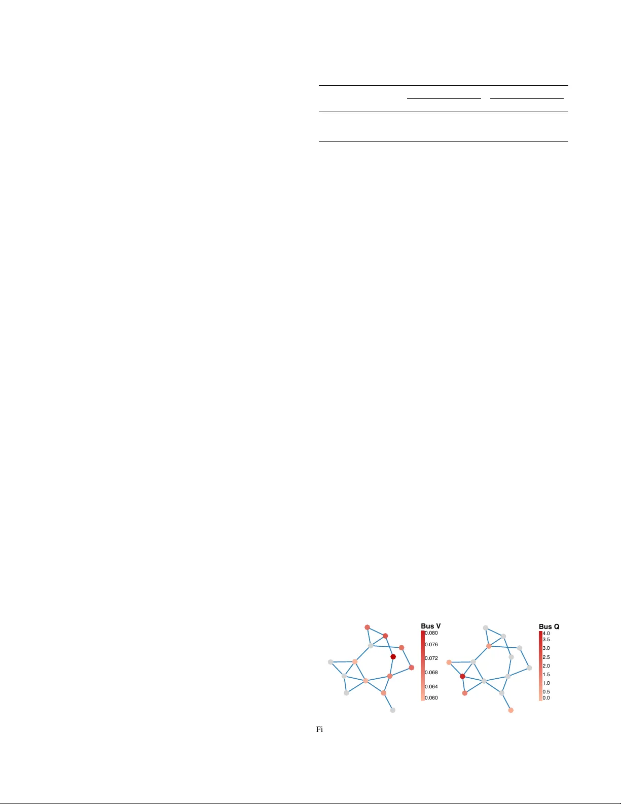
1 Generating adversarial inputs f or a graph neural network model of A C power flo w Robert Park er † Abstract —This work f ormulates and solves optimization pr ob- lems to generate input points that yield high errors between a neural netw ork’ s pr edicted A C power flow solution and solutions to the A C power flow equations. W e demonstrate this capability on an instance of the CANOS-PF graph neural network model, as implemented by the PF ∆ benchmark library , operating on a 14-bus test grid. Generated adversarial points yield errors as large as 3.4 per -unit in reacti ve power and 0.08 per -unit in voltage magnitude. When minimizing the perturbation from a training point necessary to satisfy adversarial constraints, we find that the constraints can be met with as little as an 0.04 per -unit perturbation in voltage magnitude on a single b us. This work motivates the dev elopment of rigorous verification and robust training methods for neural network surrogate models of A C power flow . Index T erms —A C Po wer Flow , Neural Networks, Optimization I . I N T RO D U C T I O N Recent work has focused on de veloping neural network surrogate models to approximate solutions to the alternating current power flow (A CPF) equations. Different architectures such as physics-informed neural netw orks (PINNs) [1], [2] and graph neural networks (GNNs) [3]–[5] ha ve been proposed and datasets such as OPF-Learn [6], OPFData [7], and PF ∆ [8] ha ve been developed to standardize comparisons among different neural (optimal) po wer flow solvers. These neural network models achieve fast online inference in exchange for a (usually) small approximation error and large offline training cost. Fast online inference is advantageous in the power transmission setting where dispatch decisions are made frequently and network topologies are generally static. Ho w- ev er, it is well-known that neural networks are not robust to adversarial perturbations [9], [10]. In safety-critical fields such as electric po wer transmission, robustness of neural network- based algorithms is especially important. This work addresses the following question: Giv en a particular surrogate model for A C power flo w , can we find input points that hav e large errors between the surrogate’ s output and a “ground truth” solution of the A C power flow equations? Our contribution is to formulate and solve two types of optimization problems for generating adv ersarial input points for an instance of the CANOS-PF graph neural network A CPF surrogate operating on the IEEE 14-bus test system from PGLib-OPF [11] and trained on data from PF ∆ . W e demonstrate that these optimization problems are tractable for a state-of-the-art embedded neural network model and that, for this model, there exist adversarial points that introduce significant discrepancies between the NN and A CPF solutions. † Los Alamos National Laboratory , Los Alamos, NM, USA LA-UR-26-20748 These points introduce large deviations in output variables that are critical for grid operators to predict accurately , such as reacti ve po wers and v oltage magnitudes. These results motiv ate further research into verification and robust training methods for neural network surrogates of A C power flow . A. Related work Many works have addressed the issue of surrogate model robustness in power system operation. Chen et al. [12] hav e identified adversarial inputs that result in misclassifications and forecasting errors, while Dinh et al. [13] have analyzed the input points that cause a multi-layer perceptron (MLP) model to make inaccurate predictions. Chev alier et al. have identified loading conditions that cause (1) a DCOPF solution to be A C-infeasible [14] and (2) an MLP’ s line switching decisions to cause high load shedding [15]. Simultaneously , methods for verification [2], robust training [16], and guaranteeing feasibility at inference time [17] of neural networks for AC power flow have been de veloped. In contrast to the “adv ersarial input” papers abov e, our work targets a graph neural network model that is state-of-the-art (according to a recent benchmark [8]). W e also impose constraints on the neural network’ s outputs (see Problem 2), which has only been done by [15]. I I . P RO B L E M F O R M U L A T I O N W e formulate and solve two types of optimization prob- lems: Maximum-error problems that maximize the dif ference between specified coordinates of the neural network’ s output and A CPF solution and constrained-err or problems that find the smallest input perturbations that satisfy constraints on each output. Each problem instance targets a specific output, such as voltage magnitude on a PV b us. In constrained-error problems, we constrain a particular output to be “sufficiently different” between the NN and A CPF solutions. The formulation of our maximum-error problem is shown in Equation 1. max ( y NN ,i − y PF ,i ) such that    y NN = NN( x ) y PF = PF( x ) L ≤ x ≤ U (1) Here, x is a vector of inputs to the A C power flo w equations: Activ e power injections and voltage magnitudes on PV buses, activ e and reactiv e po wers on PQ buses, and voltage angle and magnitude on the reference bus. Function NN ev aluates the neural network. V ector y NN contains the outputs predicted by the neural network: Reactive powers and voltage angles at PV buses, voltage angles and magnitudes at PQ buses, and activ e and reactiv e power at the reference bus. Function PF solves the A C power flow equations and returns y PF , the same outputs, now determined by these equations. Bounds on the 2 input vector ensure this problem remains bounded. Problem 1 maximizes the difference between the i -th coordinate of the neural network’ s output and the i -th coordinate of the AC power flo w equations’ output. W e solve instances of Problem 1 with both maximization and minimization objecti ve senses to maximize both the positive and negati ve errors between the neural network’ s output and the po wer flow equations’ output. The formulation of our constrained-error problem is gi ven by Problem 2. min ∥ x − x 0 ∥ 1 such that    y NN = NN( x ); y NN ,i ≥ l i y PF = PF( x ); y PF ,i ≤ l i − δ L ≤ x ≤ U (2) V ector x 0 is a reference point obtained from the training data of our surrogate model. W e use constraints to enforce a minimum difference specified by the constant parameter δ between the i -th coordinate of the neural network and power flow output vectors. Constant parameter l i emulates a lower bound that would typically be applied to this output in an optimal power flo w problem, such as a lower bound on a voltage magnitude output. Adversarial points identified by Problem 2 can be interpreted as points where the neural network predicts a feasible output (according to the bound l i in the selected coordinate) but solving the AC power flo w equations yields a solution that violates this bound by a margin of at least δ . I I I . T E S T P R O B L EM W e solve instances of Problems 1 and 2 with an imple- mentation of the CANOS-PF graph neural network operating on a 14-bus test grid. (See [5] for details on the CANOS architecture; we use the open-source CANOS-PF GNN model implemented by PF ∆ [8].) W e use the hyperparameters sug- gested by [8]: A hidden dimension of 128, 15 message passing steps, a learning rate of 10 − 5 , and 50 training epochs. The model has approximately 7.5 million trainable parameters. W e use the IEEE 14-bus test network from PGLib-OPF [11]. Input bounds are taken from the default PGLib test case. In the constrained-error problem, our output constraints target voltage magnitude at a specified PQ bus. W e use the lower bound provided by the PGLib test case and a margin of δ = 0 . 04 (per-unit). While the input vector , x , contains net loads on PQ buses, we use the con vention from PowerModels [18] that loads are non-dispatchable and are therefore fixed to their nominal values (the default PGLib v alues in the case of Problem 1 and the values from the training data point x 0 in the case of Problem 2). Similarly , we fix inputs corresponding to reference bus voltage angle and magnitude to zero and 1.0 (per-unit). This significantly constrains the feasible space of these optimization problems. Degrees of freedom are net acti ve power injections and voltage magnitudes at PV b uses. I V . C O M P U TA T I O N A L R E S U LT S W e use PF ∆ ’ s CANOS-PF model implementation, dataset, and training script. W e use the T ask-1.1 training dataset, which provides 48,600 input and output points representing solved po wer flow instances on the full network topology (no T ABLE I L O SS E S O B T A I NE D B Y O U R T R A I NE D C A N O S- P F M O D EL Dataset N. points MSE PBL Mean Stdev . Max. Mean Stdev . Max. T rain 48,600 8e-4 1e-5 9e-4 4e-2 2e-4 4e-2 T est 200 7.2 8.0 58.7 0.7 0.4 1.8 Adversarial 92 0.8 0.9 5.8 0.3 0.1 0.6 contingencies). W e implement the optimization problem using JuMP [19] and MathProgIncidence.jl [20]. PowerModels [18] implements the AC power flow constraints and MathOptAI.jl [21] implements the neural network constraints by interfacing with PyT orch [22] via a gray-box formulation [23], [24]. W e solve optimization problems (locally) with IPOPT [25] using MA57 [26] as the linear solver , a tolerance of 10 − 6 , an “acceptable tolerance” of 10 − 4 , and an iteration limit of 500. All computational experiments, including neural network training, were performed on a MacBook Pro with an M1 processor and 32 GB of RAM. A. Neural network training r esults W e train the CANOS-PF model with the PF ∆ T ask-1.1 training dataset and script for 50 epochs with a learning rate of 5 × 10 − 4 . T raining uses a combination of mean-squared-error (MSE) loss, a supervised measure, and “constraint violation loss, ” an unsupervised measure that penalizes violation of the A C power flow equations. See [27] for details behind this combined loss and [5] for the particular implementation in CANOS. Follo wing [8], we ev aluate the quality of our trained neueral network with MSE loss and “po wer balance loss” (PBL), an unsupervised measure that penalizes only violation of activ e and reactive power balance constraints. Loss values on train and test data are sho wn in T able I. These v alues are comparable to MSE and PBL losses reported by [8], so we conclude that we have accurately reproduced this work’ s CANOS-PF model. (Compare our training MSE loss to T able A.7 and our test PBL to T able A.8 in [8].) W e note that the high loss values reported for the test dataset in T able I are not surprising: T ask-1.1 training data only includes solutions for the full network topology while test data includes N − 1 and N − 2 contingenc y cases as well. The “ Adversarial” dataset in T able I refers to the adversarial points generated by solving Problems 1 and 2: 27 points from Problem 1 and 65 points from Problem 2. The generation of these points is discussed in Sections IV -B and IV -C. 0.060 0.064 0.068 0.072 0.076 0.080 Bus V 0.0 0.5 1.0 1.5 2.0 2.5 3.0 3.5 4.0 Bus Q Fig. 1. Maximum absolute error obtained for each bus. Left: PQ buses. Right: PV and reference buses. In each case, the opposite set of buses is shaded gray . Generated using PowerPlots [28]. 3 B. Maximum-err or r esults W e solve two instances of Problem 1 for each bus: One maximizing ( y NN ,i − y PF ,i ) and one minimizing the same quantity . For PQ b uses, the target output (coordinate i ) is voltage magnitude, v ; for PV and reference buses, the tar get output is reacti ve power , q . These errors we achieve are illustrated in Figure 1, where the maximum absolute values between maximization and minimization errors are displayed. The results for both maximization and minimization problems are displayed in Figure 2. 4 5 7 9 10 11 12 13 14 Bus 0 . 00 0 . 02 0 . 04 0 . 06 0 . 08 v error (p er-unit) PQ Buses    min  y NN ,i − y PF ,i        max  y NN ,i − y PF ,i     1 2 3 6 8 Bus 0 1 2 3 q error (p er-unit) PV + Reference Buses    min  y NN ,i − y PF ,i        max  y NN ,i − y PF ,i     Fig. 2. Errors achieved by Problem 1 with maximization and minimization objectiv e senses. Maximized error is omitted for bus 3 because the optimiza- tion algorithm failed to con verge for this case. The results indicate that large errors between the neural network and A C po wer flow solutions can be found. V oltage magnitude errors appear to be systematically larger when maximizing than when minimizing, suggesting that the neu- ral network has difficulty approximating solutions accurately when the power flow solution yields a relatively low voltage. W e note that solutions to the A C power flow equations are not necessarily unique, so these large errors do not necessarily indicate an incorrect prediction on the part of the neural network. Howe ver , our adv ersarial points hav e unsupervised power balance losses that are an order of magnitude higher than training data points (see T able I) — the minimum loss across these points is 0.1, indicating that our adversarial points do lead to inaccurate A C power flow solutions. W e also note that, for operating conditions of interest, AC power flow solutions are often unique. As we bound our input variables within the domains provided by PGLib, we conjecture that significant differences between neural network predictions and A C power flow solutions are a cause for concern regarding the use of this neural network model (as we hav e currently trained it) in downstream applications. T ABLE II S U MM A RY O F A DV E R S AR I A L P E RT U RB A T I O N S B Y T R A I NI N G P O I NT T raining point Con verged A verage index (of 9) ∥ x − x 0 ∥ 1 ∥ x − x 0 ∥ 0 y NN ,i y PF ,i 0 9 0.31 3 0.96 0.90 1 6 0.19 2 0.96 0.90 2 8 0.13 3 0.96 0.90 3 5 0.11 2 0.96 0.90 4 6 0.09 2 0.95 0.90 5 7 0.20 2 0.96 0.90 6 8 0.13 2 0.95 0.90 7 6 0.25 3 0.96 0.90 8 3 0.15 4 0.94 0.90 9 7 0.18 2 0.95 0.90 C. Constrained-err or results W e solve instances of Problem 2 for each of nine PQ buses and for the first ten training points of the PF ∆ T ask-1.1 dataset. T able II summarizes the results by training point. W e first note that all PQ b uses hav e voltage magnitude lower bounds (according to PGLib) of 0.94, so our constraint on y PF ,i (with margin δ = 0 . 04 ) is always y PF ,i ≤ 0 . 90 . The errors in voltage magnitude we achie ve range from 0.04 to 0.06. There is a large variation in the number of successfully con ver ged problems for different training points, suggesting that some training points are more vulnerable to adversarial perturbations than others. Overall, 65 / 90 instances con verge to primal-feasible points. T ABLE III A DV E RS A R I AL P E RTU R BAT IO N S F O R S E LE C T E D C A S E S Training T argeted ∥ x − x 0 ∥ 1 ∥ x − x 0 ∥ 0 V ariables point bus 4 12 0.04 1 v 6 = 0 . 96 0 4 0.18 2 v 2 = 0 . 94 , v 3 = 0 . 95 8 7 0.14 3 v 2 = 0 . 95 , v 6 = 1 . 03 , v 8 = 0 . 94 9 9 0.30 4 v 2 = 0 . 94 , v 3 = 1 . 00 , v 6 = 0 . 94 , v 8 = 1 . 02 2 4 0.11 5 v 1 = 1 . 00 , v 2 = 0 . 95 , v 3 = 1 . 00 , v 6 = 1 . 02 , v 8 = 1 . 04 0 . 0 0 . 1 0 . 2 0 . 3 0 . 4 0 . 5 0 . 0 2 . 5 5 . 0 7 . 5 10 . 0 12 . 5 15 . 0 Count 0 . 9 1 . 0 1 . 1 k x − x 0 k 1 Fig. 3. Histogram of l 1 perturbation magnitudes necessary to satisfy adver- sarial constraints. The “0-norm” in T able II is the number of nonzero entries of its ar gument, i.e., the number of input variables that need to be perturbed to achiev e the adversarial outcome. W e note that these numbers are low: In most cases, the adversarial outcome is achie ve by perturbing only two input variables. Particular variables perturbed in selected cases are sho wn in T able III and Figure 3 shows a histogram of perturbation 1- 4 norms required to satisfy the adversarial constraints. As shown in T able III, these perturbations often require setting voltage magnitude on PV buses to a v alue close to its lo wer bound of 0.94. This result suggests that robustness of the CANOS-PF neural network model could be improved by including more points with output v oltages near this bound in the training data. W e leave such improvements to the neural network model for future work. V . C O N C L U S I O N This work is a proof-of-concept that adversarial points can be systematically identified for a state-of-the-art neural network model of A C power flow . W e have demonstrated the method on a small, 14-bus test system, but we believ e the method will apply to larger systems as well. The results of Shin et al. [29] show that interior point methods, such as the IPOPT algorithm we use here, can solve problems with large-scale power networks while our prior results [24] sho w that these methods can solve problems with large-scale neural network models. Additionally , we note that by keeping loads fixed, we ha ve significantly constrained the input space that we search for adv ersarial points. W orse points than those shown here can likely be generated if loads (and line parameters) are used as degrees of freedom as well. W e belie ve this work motiv ates the need for continued robustness testing of neural network surrogate models for AC power flow , de velopment of rigorous validation methods for these models, and dev elopment of adversarially robust training and inference methodologies. A C K N O W L E D G E M E N T S AI was used to write scripts to generate some of the figures and tables presented in this work after the raw data had been generated by a human programmer . R E F E R E N C E S [1] R. Nellikkath and S. Chatziv asileiadis, “Physics-informed neural net- works for A C optimal power flow , ” Electric P ower Systems Research , vol. 212, p. 108412, 2022. [2] J. Jalving, M. Eydenberg, L. Blakely , A. Castillo, Z. Kilwein, J. K. Skolfield, F . Boukouvala, and C. Laird, “Physics-informed machine learning with optimization-based guarantees: Applications to AC power flow , ” International Journal of Electrical P ower & Ener gy Systems , vol. 157, p. 109741, 2024. [3] B. Donon, R. Cl ´ ement, B. Donnot, A. Marot, I. Guyon, and M. Schoe- nauer , “Neural networks for power flow: Graph neural solver, ” Electric P ower Systems Researc h , vol. 189, p. 106547, 2020. [4] N. Lin, S. Orfanoudakis, N. O. Cardenas, J. S. Giraldo, and P . P . V ergara, “PowerFlo wNet: Po wer flow approximation using message passing graph neural networks, ” International J ournal of Electrical P ower & Energy Systems , vol. 160, p. 110112, 2024. [5] L. Piloto, S. Liguori, S. Madjiheurem, M. Zgubic, S. Lov ett, H. T om- linson, S. Elster , C. Apps, and S. Witherspoon, “CANOS: A fast and scalable neural AC-OPF solver robust to N-1 perturbations, ” 2024. [6] T . Joswig-Jones, K. Baker, and A. S. Zamzam, “OPF-Learn: An open- source framework for creating representative AC optimal po wer flow datasets, ” in 2022 IEEE P ower & Ener gy Society Innovative Smart Grid T echnologies Conference (ISGT) , pp. 1–5, 2022. [7] S. Lovett, M. Zgubic, S. Liguori, S. Madjiheurem, H. T omlinson, S. Elster , C. Apps, S. Witherspoon, and L. Piloto, “OPFData: Lar ge- scale datasets for ac optimal power flow with topological perturbations, ” 2024. [8] A. K. Riv era, A. Bhagav athula, A. Carbonero, and P . L. Donti, “PF ∆ : A benchmark dataset for power flow under load, generation, and topology variations, ” in The Thirty-ninth Annual Conference on Neural Information Pr ocessing Systems Datasets and Benchmarks T rack , 2025. [9] C. Szegedy , W . Zaremba, I. Sutske ver , J. Bruna, D. Erhan, I. Good- fellow , and R. Fergus, “Intriguing properties of neural networks, ” in International Conference on Learning Repr esentations , 2014. [10] R. R. W iyatno, A. Xu, O. Dia, and A. de Berker , “ Adversarial examples in modern machine learning: A revie w , ” 2019. [11] S. Babaeinejadsarookolaee, A. Birchfield, R. D. Christie, C. Cof frin, C. DeMarco, R. Diao, M. Ferris, S. Fliscounakis, S. Greene, R. Huang, C. Josz, R. Korab, B. Lesieutre, J. Maeght, T . W . K. Mak, D. K. Molzahn, T . J. Overbye, P . Panciatici, B. Park, J. Snodgrass, A. Tbaileh, P . V . Hentenryck, and R. Zimmerman, “The po wer grid library for benchmarking AC optimal power flow algorithms, ” 2021. [12] Y . Chen, Y . T an, and D. Deka, “Is machine learning in power systems vulnerable?, ” in 2018 IEEE International Conference on Communica- tions, Control, and Computing T echnologies for Smart Grids (Smart- GridComm) , pp. 1–6, 2018. [13] M. H. Dinh, F . Fioretto, M. Mohammadian, and K. Baker, “ An analysis of the reliability of A C optimal power flow deep learning proxies, ” in 2023 IEEE PES Innovative Smart Grid T echnologies Latin America (ISGT -LA) , pp. 170–174, 2023. [14] S. Chevalier and W . A. Wheeler, “Identifying the smallest adversarial load perturbation that renders dc-opf infeasible, ” IEEE T ransactions on P ower Systems , pp. 1–12, 2026. [15] S. Chev alier , D. Starkenburg, R. Parker , and N. Rhodes, “Maximal load shedding verification for neural network models of ac line switching, ” 2025. [16] B. Giraud, R. Nellikath, J. V orwerk, M. Alowaifeer , and S. Chatzi- vasileiadis, “Neural networks for A C optimal power flow: Improving worst-case guarantees during training, ” 2025. [17] P . L. Donti, D. Rolnick, and J. Z. Kolter , “DC3: A learning method for optimization with hard constraints, ” in International Confer ence on Learning Representations , 2021. [18] C. Coffrin, R. Bent, K. Sundar , Y . Ng, and M. Lubin, “PowerModels.jl: An open-source framew ork for exploring power flow formulations, ” in 2018 P ower Systems Computation Confer ence (PSCC) , pp. 1–8, June 2018. [19] M. Lubin, O. Dowson, J. D. Garcia, J. Huchette, B. Legat, and J. P . V ielma, “JuMP 1.0: Recent improv ements to a modeling language for mathematical optimization, ” Mathematical Pr ogramming Computation , vol. 15, no. 3, pp. 581–589, 2023. [20] R. B. Parker , B. L. Nicholson, J. D. Siirola, and L. T . Biegler , “ Applications of the Dulmage-Mendelsohn decomposition for deb ugging nonlinear optimization problems, ” Computers & Chemical Engineering , vol. 178, p. 108383, 2023. [21] O. Dowson, R. B. Parker , and R. Bent, “MathOptAI.jl: Embed trained machine learning predictors into JuMP models, ” 2025. [22] A. Paszke, S. Gross, F . Massa, A. Lerer, J. Bradbury , G. Chanan, T . Killeen, Z. Lin, N. Gimelshein, L. Antiga, et al. , “Pytorch: An imperativ e style, high-performance deep learning library , ” Advances in neural information pr ocessing systems , vol. 32, 2019. [23] C. A. Elorza Casas, L. A. Ricardez-Sandov al, and J. L. Pulsipher, “ A comparison of strategies to embed physics-informed neural networks in nonlinear model predictive control formulations solved via direct transcription, ” Computers & Chemical Engineering , vol. 198, p. 109105, 2025. [24] R. B. Parker , O. Do wson, N. LoGiudice, M. J. Garcia, and R. Bent, “Nonlinear optimization with GPU-accelerated neural network con- straints, ” in NeurIPS W orkshop on GPU-Accelerated and Scalable Optimization , 2025. [25] A. W ¨ achter and L. T . Biegler , “On the implementation of an interior- point filter line-search algorithm for large-scale nonlinear programming, ” Mathematical progr amming , vol. 106, no. 1, pp. 25–57, 2006. [26] I. S. Duff, “MA57—a code for the solution of sparse symmetric definite and indefinite systems, ” vol. 30, no. 2, 2004. [27] F . Fioretto, T . W . Mak, and P . V an Hentenryck, “Predicting A C optimal power flows: Combining deep learning and lagrangian dual methods, ” Pr oceedings of the AAAI Confer ence on Artificial Intelligence , vol. 34, pp. 630–637, Apr . 2020. [28] N. Rhodes, “PowerPlots.jl: An open source power grid visualization and data analysis framework for academic research, ” 2025. [29] S. Shin, M. Anitescu, and F . Pacaud, “ Accelerating optimal po wer flow with GPUs: SIMD abstraction of nonlinear programs and condensed-space interior-point methods, ” Electric P ower Systems Re- sear ch , vol. 236, p. 110651, 2024.