Learning from Biased and Costly Data Sources: Minimax-optimal Data Collection under a Budget

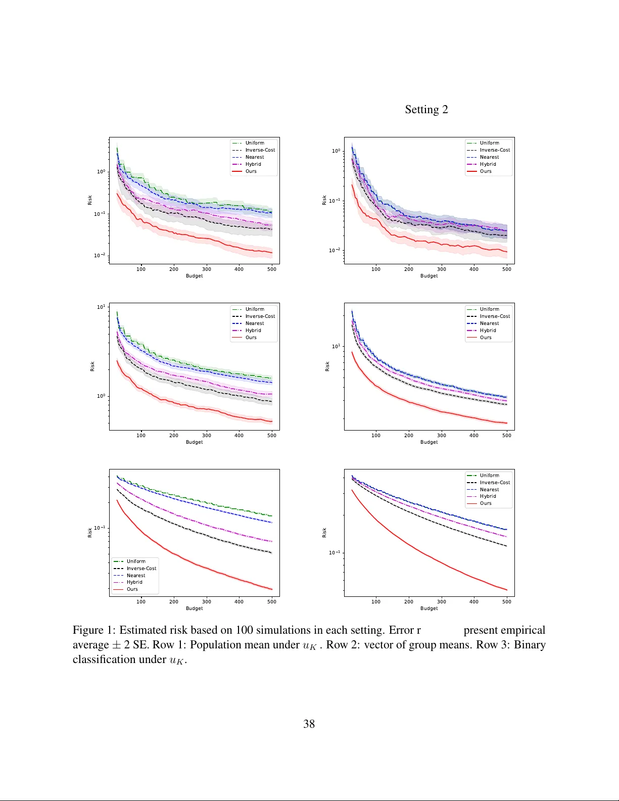
Learning from Biased and Costly Data Sources: Minimax-optimal Data Collection under a Budget Michael O. Harding Uni versity of W isconsin-Madison moharding@wisc.edu V ikas Singh Uni versity of W isconsin-Madison vsingh@biostat.wisc.edu Kirthe v asan Kandasamy Uni versity of W isconsin-Madison kandasamy@cs.wisc.edu Abstract Data collection is a critical component of modern statistical and machine learning pipelines, particularly when data must be gathered from multiple heterogeneous sources to study a target population of interest. In many use cases, such as medical studies or political polling, dif ferent sources incur dif ferent sampling costs. Observations often hav e associated group identities—for example, health markers, demographics, or political afﬁliations—and the relati v e composition of these groups may differ substantially , both among the source populations and between sources and target population. In this work, we study multi-source data collection under a ﬁxed budget, focusing on the estimation of population means and group-conditional means. W e show that naive data collection strategies (e.g. attempting to “match” the target distribution) or relying on standard estimators (e.g. sample mean) can be highly suboptimal. Instead, we dev elop a sampling plan which maximizes the ef fective sample size —the total sample size di vided by D χ 2 ( q || p ) + 1 , where q is the target distribution, p is the aggregated source distributions, and D χ 2 is the χ 2 - di ver gence. W e pair this sampling plan with a classical post-stratiﬁcation estimator and upper bound its risk. W e provide matching lower bounds, establishing that our approach achieves the b udgeted minimax optimal risk. Our techniques also extend to prediction problems when minimizing the excess risk, pro viding a principled approach to multi-source learning with costly and heterogeneous data sources. 1 Intr oduction Data collection is a central component of an y data analysis pipeline. The performance of e v en the most well-designed estimators (or learning algorithms) depends hea vily on the data the y are trained on, and thus the design of the data collection scheme can be just as important as the estimator itself. 1 Multi-source data collection In many practical scenarios, data is collected from multiple sour ces in service of designing a system to better understand a tar get population of interest. For example, planners of a clinical study may w ork with a number of treatment centers (sources) spread across a country , with the goal of predicting treatment ef fects across the entire population (target) of their country . Complicating this process is the heterogeneity in the distrib ution of gr oups , such as demographics or disease pre v alence, at the sources, and the data collection costs at each source. These groups often v ary substantially across centers and dif fer markedly from those of the o verall population, and costs of data collection can vary due to operational expenses and participant recruitment. Most results in the statistics and machine learning literature rely on the assumption that the training data come from the same tar get distribution ag ainst which an estimator will be e valuated. Thus, when faced with the problem of designing a data collection system with access to multiple, heterogeneous data sources, at ﬁrst glance, it w ould appear that the goal should be to craft a sampling scheme which results in an aggregated “source” which most closely resembles the target distribution of interest. Ho wev er , this naiv e approach ignores differences in sampling costs across sources, and fails to e xploit the fact that a well-designed estimator should beneﬁt from additional data. On the other hand, simply maximizing the number of collected samples without regard to the tar get distribution is also not meaningful. W e illustrate these challenges via the e xample below . Example. W e wish to estimate the av erage BMI of adults in a state where it is kno wn that 25% of adults are physically acti ve (A) and 75% are inacti ve (I). Collecting i.i.d. samples from the population would permit direct estimation via the sample mean. Howe ver , data must be collected from one of two sources, an urban and rural clinic, under a ﬁxed b udget of $1,000. Measuring BMI costs $1 and $2 per sample at the urban and rural clinics, respecti v ely . The urban population is 80% acti ve , while the rural population matches the state (25% acti ve), reﬂecting strong selection ef fects. Crucially , an indi vidual’ s activity status is unkno wn at recruitment, requiring a post-measurement questionnaire. Allocating the entire b udget to the urban clinic yields 1,000 measurements, b ut only roughly 200 from group I, which represents the majority of the population of interest. Another naiv e approach attempting to “match” the state distrib ution would allocate the entire b udget to the rural clinic, yielding 500 measurements matching the state (roughly 125 from A and 375 from I), and use the sample mean. Ho we ver , using the techniques we dev elop, the optimal allocation turns out to be collecting 152 and 424 samples from the urban and rural clinics, respectiv ely , yielding roughly 228 samples from A and 348 samples from I. While there is a mismatch with the state population, collecting more data from group A (relati ve to “matching”) is more helpful here. Though the sample mean is no longer appropriate, pairing this with an appropriate estimator could le verage the larger , albeit biased, sample to improv e estimation accuracy . This example highlights se veral key features of multi-source data collection: (i) Sampling from dif ferent sources incurs dif ferent costs. (ii) Source populations hav e heterogeneous group compositions that can dif fer substantially from the target population. (iii) Group proportions are known , both at the source and target levels, but it is not always possible to cheaply preselect indi viduals based on group identity 1 . (iv) Ef fecti ve data collection must be paired with a well- 1 In practice, planners of clinical studies may ha ve already pre-selected ba sed on easily observable characteristics 2 designed estimator that can appropriately le verage large but systematically biased datasets. These challenges moti vates the follo wing question of study for this setting: What is the optimal pr ocedur e for collecting and learning fr om data coming fr om sources with heter o geneous population compositions and unequal data collection costs? 1.1 Model En vir onment A population can be di vided into K groups. A planner has access to M sources, from which they can sample data. Observations are in the form of a tuple ( Z, Y ) , where Z ∈ [ K ] = { 1 , . . . , K } is the group identity and Y ∈ R is the response, or label. At source m , we assume ( Z, Y ) iid ∼ P m ( z , y ) = p m ( z ) P Y | Z ( y | z ) . Here, p m is a known discrete distrib ution over [ K ] , deﬁning the group distribution at source m , while P Y | Z is an unknown conditional distribution. All groups hav e positi ve probability in at least one source, i.e. for each z ∈ [ K ] , there exists m ∈ [ M ] such that p m ( z ) > 0 . W e assume that P Y | Z does not depend on the source m ; this assumption is reasonable in practice with sufﬁciently informati ve groups (e.g., treatment response is independent of location, conditional on disease condition, genetic markers, age, etc.), while still yielding a rich theoretical frame work. W e also assume that P Y | Z belongs to the follo wing class: P Y | Z :=  P Y | Z ∈ P ( R ) : | E [ Y | Z ] | ≤ R , V ar( Y | Z ) ≤ σ 2 , a.s.  , where P ( R ) is the set of all probability distrib utions ov er R . Here, R and σ 2 are unknown to the policy . As we show in Theorem 6 , boundedness of | E [ Y | Z ] | is necessary in this problem. Learning with r espect to a target gr oup distribution In this work, we focus mainly on estimating (i) the mean or (ii) the vector of conditional means. W e formulate (i) as estimating the expectation of Y , under the squared loss, for a tar get distrib ution Q of interest. The target distrib ution can be written as Q ( z , y ) = q ( z ) P Y | Z ( y | z ) ; here q is known , and deﬁnes the distrib ution of groups at the population le vel, and the conditional distribution P Y | Z is unkno wn and the same as the sources. The population mean is θ PM ( Q ) = E Y ∼ Q [ Y ] , where θ PM : P Y | Z → R . For (ii) , we deﬁne the group-conditional means as θ GM ( Q ) = { E Y ,Z ∼ Q [ Y | Z = z ] } z ∈ [ K ] , where θ GM : P Y | Z → R K , which we will estimate under the ℓ 2 2 loss; as we will see, estimating the conditional means can be framed as estimation under a “uniform” target distrib ution. These two parameters co ver a broad range of quantities of interest to practitioners. The popula- tion mean corresponds to quantities such as the av erage treatment effect (A TE) ( Hirano et al. , 2003 ; Imbens , 2004 ; Chernozhukov et al. , 2018 ) of a new therapeutic, proportion of v otes for a candidate, or the e xpected re venue for a new product across an entire customer base. Like wise, the vector of conditional means corresponds to quantities such as the conditional average treatment ef fect (CA TE) ( Imai and Ratkovic , 2013 ; W ager and Athey , 2018 ; Nie and W ager , 2021 ), the proportion of votes in each demographic group, or the e xpected re venue within each customer se gment. (e.g., age or race), while identifying other group attrib utes requires incurring the measurement cost (e.g., health conditions). 3 Multi-source data collection under a b udget In practice, there are important resource constraints to consider when collecting data. T raditionally , this is studied via the performance of the system in terms of the total sample size, b ut this only serves as a proxy for the actual constraints, such as time and/or money needed to sample data. T o this end, we study the setting where each sample from source m comes at a cost c m , and so the total cost of a sampling plan n = ( n 1 , . . . , n M ) , where n m is the number of points to be collected from source m , is c ⊤ n , for c = ( c 1 , . . . , c M ) . W e hav e a ﬁxed b udget B > 0 , and feasible sampling plans are those which satisfy c ⊤ n ≤ B . For population mean estimation, a policy is a tuple ( n , b θ PM ) , consisting of both a sampling plan n and an estimator b θ PM mapping the collected data D to an estimate b θ PM ( D ) . The risk of a polic y under the (unkno wn) conditional distribution P Y | Z is the expected squared loss: R PM (( n , b θ PM ) , P Y | Z ) := E D ∼ P n   b θ PM ( D ) − θ PM ( Q )  2 2  . Here, P n denotes the joint distrib ution of data collected from the sources under the sampling plan n . For simplicity , we suppress the dependence of the risk on the group distributions p m and q , which are ﬁxed and kno wn to the planner ahead of time. A policy’ s performance is e v aluated relati ve to the b udgeted minimax risk R ⋆ PM , deﬁned below . Note that the supremum is taken only over the conditional distributions P Y | Z which is the only unkno wn. W e hav e: R ⋆ PM ( B , P Y | Z ) := inf c ⊤ n ≤ B inf b θ PM sup P Y | Z ∈P Y | Z R PM (( n , b θ PM ) , P Y | Z ) , (1) For estimating group-conditional means, a policy is similarly a tuple ( n , b θ GM ) . The risk of a planner’ s policy R GM is as deﬁned belo w , with the minimax risk deﬁned similar to ( 1 ). W e hav e: R GM (( n , b θ GM ) , P Y | Z ) := E D ∼ P n     b θ GM ( D ) − θ GM ( Q )    2 2  . 1.2 Summary of our contrib utions and techniques W e ﬁrst establish lo wer bounds on the minimax risks for this no vel setting, and then design minimax optimal policies. W e then extend these ideas to prediction tasks. W e no w outline our main contributions, focusing on population mean estimation for simplicity . Effective sample size A k ey quantity in our analysis is the effective sample size , which quantiﬁes ho w well we can estimate a population quantity when data comes from dif ferent sources. T o deﬁne this, for a sampling plan n , let p n = ( 1 ⊤ n ) − 1 P M m =1 n m p m be the mixture distribution ov er the group identities. For a ﬁx ed set of source group distributions { p m } m ∈ [ M ] , we deﬁne the effecti v e sample size n eﬀ ( n , q ) for a sampling plan n with respect to a target distribution q over groups as: n eﬀ ( n , q ) := 1 ⊤ n d ( q || p n ) , where, d ( a || b ) := X z ∈ [ K ] a 2 ( z ) b ( z ) . (2) 4 That is, the ef fecti ve sample size is the total number of samples collected di vided by the discrepanc y measure d ( q || p n ) . The discrepanc y measure satisﬁes d ( a || b ) ≥ 1 , with equality only when a = b . It also satisﬁes d ( a || b ) = exp( D 2 ( a || b )) = D χ 2 ( a || b ) + 1 , where D 2 is the Rényi-2 di ver gence ( Rényi , 1961 ) and D χ 2 is the χ 2 di ver gence. Lower bound (§ 2 ) Our ﬁrst result establishes a lower bound on the risk achie vable by an y policy . As we will see, this lo wer bound also informs the design of an optimal policy for this problem. T o state the result, deﬁne c ( n ) = ( 1 ⊤ n ) − 1 c ⊤ n as the avera ge sample cost of a sampling plan n . Theorem 1 (Informal) . The minimax risk ( 1 ) satisﬁes the following lower bound, wher e n ⋆ T is the sampling plan n which maximizes n eﬀ ( n , q ) subject to the constraint c ⊤ n ≤ B . W e have, R ⋆ PM ( B , P Y | Z ) ≥ σ 2 c ( n ⋆ T ) d ( q || p n ⋆ T ) B − o  1 B  = σ 2 n eﬀ ( n ⋆ T , q ) − o  1 B  , The lo wer bound illustrates that the ef fecti ve sample size is a k ey quantity in this problem, as we see the familiar σ 2 /n bound on the risk, except with n replaced by the ef fectiv e sample size of n ⋆ T . Pr oof outline. The proof, which is a ke y technical contribution of this work, builds on the common technique of lo wer bounding the worst-case risk o ver P Y | Z by the expected risk of the Bayes estimator under a suitably chosen prior . Howe v er , the typical choice for this technique, le veraging normal-normal conjugac y , does not work in our setting, as we assume a bounded domain for the means (recall that the problem is hopeless without boundedness). W e instead utilize a uniform prior , requiring study of the expected v ariance of a truncated normal posterior distribution. W e then recover appropriate dependence on n eﬀ ( n , q ) via a decomposition of an intractable integral appearing in the posterior v ariance into 3 regions, carefully chosen to le v erage normal distribution properties and a Gaussian tail lo wer bound technique. Upper bound (§ 3 ) This lower bound, if tight, suggests collecting data according to the sampling plan n ⋆ T and pairing it with an appropriate estimator to obtain a minimax-optimal policy . The sample mean is inadequate here, since the mixture distrib ution induced by n ⋆ T generally dif fers from the target distrib ution. Instead, we sho w that the natural and classically studied post-stratiﬁed estimator b θ PS ( Holt and Smith , 1979 ), which ﬁrst estimates the mean within each group { Y z } z ∈ [ K ] and then combines them as P z ∈ [ K ] q ( z ) Y z , is optimal for this setting. This yields the follo wing theorem. Theorem 2 (Informal) . The policy ( n ⋆ T , b θ PS ) achie ves risk, R PM (( n ⋆ T , b θ PS ) , P Y | Z ) ≤ σ 2 c ( n ⋆ T ) d ( q || p n ⋆ T ) B + o  1 B  = R ⋆ PM ( B , P Y | Z ) + o  1 B  This result matches the lo wer bound with exact constants in the leading term, establishing that ( n ⋆ T , b θ PS ) is minimax optimal. While relying on standard tools—a careful decomposition of the risk and T aylor expansion to control lo wer -order terms—this proof is nonetheless nov el, dif fering fundamentally from prior analyses of the post-stratiﬁed estimator . 5 Prediction problems (§ 4 ) Next, we explore prediction problems where we hav e additional features X , associated with each observation, separate from the group identity Z . Giv en a hypothesis class H consisting of hypotheses mapping ( Z, X ) to a label Y , we wish to collect data, and use it to ﬁnd a hypothesis h ∈ H which minimizes the prediction error with respect to a gi ven tar get distribution. Upper bound. W e ﬁrst study ho w our sampling plan, which maximizes the ef fecti v e sampling size, performs when paired with an Importance-W eighted Empirical Risk Minimization (IWERM) procedure b h IWERM ( Cortes et al. , 2010 ). W e hav e the following bound on the excess risk of our method R Pr (( n ⋆ T , b h IWERM ) , H ) (i.e. risk of our method minus the best achiev able in H ). Theorem 3 (Informal) . Suppose the hypothesis class H ⊂ { h : [ K ] × X → R } , when r estricted to any z ∈ [ K ] , has ﬁnite pseudo-dimension Pdim( H ) over X . Then, under a budget B , the e xcess risk of our policy ( n ⋆ T , b h IWERM ) can be upper bounded by R Pr (( n ⋆ T , b h IWERM ) , H ) ∈ e O   s Pdim( H ) K c ( n ⋆ T ) d ( q || p n ⋆ T ) B   Lower bound. T o study if our sampling plan is optimal in a prediction setting, we establish lo wer bounds for binary classiﬁcation under the 0–1 loss, where the pseudo-dimension is simply the VC dimension ( V apnik and Chervonenkis , 1971 ; Pollard , 1984 ). This giv es us the follo wing result on the minimax excess risk R ⋆ Pr ( B , H ) relati v e to a hypothesis class H under a budget B . Theorem 4 (Informal) . Suppose the hypothesis class H ⊂ { h : [ K ] × X → {± 1 }} , when restricted to any z ∈ [ K ] , has ﬁnite VC-dimension V Cdim( H ) over X . Let q min = min z ∈ [ K ] q ( z ) . Then, the minimax excess risk satisﬁes R ⋆ Pr ( B , H ) ∈ Ω   s V Cdim( H ) q min c ( n ⋆ T ) d ( q || p n ⋆ T ) B   Comparing with the upper bound, we hav e matching dependence on V Cdim( H ) n − 1 eﬀ ( n ⋆ T , q ) , indicating that the effecti v e sample size is a fundamental quantity in this setting as well. While there is a p K/q min gap between the upper and lo wer bounds, we belie ve this is an artifact of our analysis. As was the case for mean estimation, the k ey technical challenge in this setting is the lower bound. Despite the wealth of related cov ariate shift literature ( Shimodaira , 2000 ; Sugiyama et al. , 2007 ; Mansour et al. , 2009 ; Cortes et al. , 2010 , 2019 ; Hannek e and Kpotufe , 2019 ; Sugiyama and Kaw anabe , 2019 ; Zhang et al. , 2020 ; Kpotufe and Martinet , 2021 ; F ang et al. , 2023 ; Ma et al. , 2023 ; Ge et al. , 2024 ), to the best of our kno wledge, we are the ﬁrst to pro vide a minimax lo wer bound for the excess risk with e xplicit dependence on the discrepancy d ( q || p n ) . Pr oof outline . The standard reduction from learning to testing to prov e lo wer bounds does not apply directly in our setting, since training data are dra wn from source distribution(s) that diff er from the tar get distrib ution under which performance is e valuated. T o address this challenge, we de velop a nov el r eduction-to-testing lemma that explicitly accounts for this distrib utional mismatch. 6 W e combine this lemma with Fano’ s inequality to obtain a general frame work for minimax lo wer bounds. The framework relates the minimax risk to (i) the separation of losses induced under the target distrib ution and (ii) the KL div ergences induced between the corresponding source distributions. T o fully e xploit this machinery and induce the desired dependence on d ( q || p n ) , we construct a family of conditional distrib utions index ed by a subset of the d -dimensional hypercube via the Gilbert–V arshamov lemma ( Gilbert , 1952 ; V arshamov , 1957 ). The construction separates positi ve and negati ve class probabilities according to the group identity z . W ith an appropriate choice of separations, the resulting class is well separated in loss under q while maintaining uniformly bounded KL di ver gences under p n , yielding the desired lo wer bound. Empirical evaluation (A pp. G ) W e corroborate our results in simulations, comparing to a set of straightforward, yet suboptimal, alternativ e sampling plans. W e demonstrate ho w they under- perform compared to our policy of maximizing the ef fecti ve sample size. 1.3 Related W ork Sampling techniques Existing methods broadly fall into the following three cate gories. Stratiﬁed sampling. The most traditional approach is stratiﬁed sampling, dating back to Ne yman ( 1934 ). Here, it is assumed that the planner can collect i.i.d. samples from each group (stratum). In our setting, this approach would require recruited indi viduals to be pre-selected based on their group identity , or each source to itself be a group. Ho we ver , it is often impossible to observ e the group identity without incurring the sampling cost, and we aim to study groups which are not uniquely deﬁned by the sources. The stratiﬁed setting is well studied and continues to attract ne w research ( Khan et al. , 2003 ; Meng , 2013 ; Khan et al. , 2015 ; Liberty et al. , 2016 ; Cervellera and Macciò , 2018 ; Sauer et al. , 2021 ; Y adav et al. , 2025 ), b ut these approaches fail to generalize to our setting. Multiple-frame sampling. Multiple-frame sampling studies the setting where the sources (frames) from which the planner is sampling cover o verlapping sub-populations. A classic example is a telephone surve y ( W olter et al. , 2015 ), where the two sources are cell phone and landline users. Some individuals will own both, so they ha ve a possibility of being selected in both sources. Optimal allocation strategies in this setting are thus focused on the size and v ariance within these intersections, which is not applicable to our setting. W e refer the reader to a thorough revie w from Lohr ( 2007 ). Cluster sampling . Of these approaches, cluster sampling is the most similar to our problem. Here, the planner collects i.i.d. samples from each source (cluster), as in our setting. Howe v er , these approaches often assume that sources are sampled from the super-population of sources, e.g. randomly selecting blocks in a city ( T ryfos , 1996 ). Instead, our setting allo ws for the common case where sources a vailable for sampling are ﬁxed a priori. Even when this assumption is not critical, optimal allocation in the cluster sampling literature does not address our setting of heterogeneous group compositions and how the y affect the design of sampling plans ( Connelly , 2003 ; Sharma and Khan , 2015 ; Shen and K elcey , 2020 ; Copas and Hooper , 2021 ; V arshney et al. , 2023 ). 7 Effective sample size W e note that our deﬁnition of the ef fecti ve sample size appears in related ﬁelds, primarily in e valuating MCMC algorithms in Bayesian importance sampling ( K ong et al. , 1994 ; Fishman , 1996 ; Liu , 1996 ; Agapiou et al. , 2017 ; Martino et al. , 2017 ; Elvira et al. , 2022 ) and in learning under co v ariate shift ( Mansour et al. , 2009 ; Cortes et al. , 2010 , 2019 ; Maia Polo and V icente , 2023 ). Further , existing lo wer bounds in the cov ariate shift literature either do not consider a ﬁxed target-source pair ( Hanneke and Kpotufe , 2019 ; Kpotufe and Martinet , 2021 ; Ma et al. , 2023 ) or do not induce dependence on d ( q || p n ) when applied to our setting ( Ge et al. , 2024 ). 2 Lower Bounds W e no w study the mean estimation problems from § 1.1 . Recall the deﬁnition of the minimax risk from ( 1 ) , and the ef fecti ve sample size n eﬀ from ( 2 ) . Let u K denote the uniform distrib ution o ver [ K ] and n z denote the (randomly) observ ed number of observ ations from group z in a dataset D . W e begin with the following lo wer bounds and a sk etch of our proof; the full version is in App. B . Theorem 1. F ix a budget B > 0 and a vector of costs c = ( c 1 , . . . , c M ) , with c m > 0 for all m ∈ [ M ] . Deﬁne the following sampling plans, n ⋆ T ∈ argmax n ∈ N M n eﬀ ( n , q ) s.t. c ⊤ n ≤ B , n ⋆ U ∈ argmax n ∈ N M n eﬀ ( n , u K ) s.t. c ⊤ n ≤ B (3) Then, we have the following lower bounds on the risk of any policy ( n , θ ) , R ⋆ PM ( B , P Y | Z ) ≥ σ 2 c ( n ⋆ T ) d ( q || p n ⋆ T ) B − O  1 B 3 / 2  = σ 2 n eﬀ ( n ⋆ T , q ) − o  1 B  R ⋆ GM ( B , P Y | Z ) ≥ K 2 σ 2 c ( n ⋆ U ) d ( u K || p n ⋆ U ) B − O  1 B 3 / 2  = K 2 σ 2 n eﬀ ( n ⋆ U , u K ) − o  1 B  Pr oof . (Proof sketch of Theorem 1 ). W e consider a mean parameter µ ∈ [ − R , R ] K and a uniform prior distribution o ver the v alue of this parameter , Π = Unif ([ − R, R ] K ) . W e consider the distri- butions P µ ∈ P Y | Z having normal conditional distrib utions with conditional mean vector µ and v ariance σ 2 ; that is, Y ∼ P µ = ⇒ Y | Z = z ∼ N ( µ z , σ 2 ) . W e ﬁrst lo wer bound the w orst-case risk by the expected risk of the Bayes estimator . Lemma 1. Consider the following generative model: ﬁrst, µ ∼ Π , then, for a sampling plan n , the dataset D ∼ P n , with P Y | Z = P µ . Further , denote by P ′ n the unconditional data distrib ution, accounting for the randomness in µ , and by Π µ | D the posterior distribution o ver µ . Then, R ⋆ PM ( B , P Y | Z ) ≥ inf c ⊤ n ≤ B X z ∈ [ K ] q 2 ( z ) E D ∼ P ′ n h V ar µ ∼ Π µ | D ( µ z | D ) i R ⋆ GM ( B , P Y | Z ) ≥ inf c ⊤ n ≤ B X z ∈ [ K ] E D ∼ P ′ n h V ar µ ∼ Π µ | D ( µ z | D ) i (3) 8 W e then study the posterior distrib ution Π µ | D . W e ﬁnd that the µ z ’ s are independent and, on the e vent n z > 0 , µ z follo ws a truncated normal distrib ution with location Y z , scale σ 2 / n z , and domain [ − R, R ] . Ne xt, we explicitly compute the density of P ′ n ( Y z | n z ) and combine it with the variance of a truncated normal distribution to arri v e at, E D ∼ P ′ n h V ar µ ∼ Π µ | D ( µ z | D ) | n z i = σ 2 n z    1 − σ 2 √ n z R Z R h ϕ  x + √ n z R σ  − ϕ  x − √ n z R σ i 2 Φ  x + √ n z R σ  − Φ  x − √ n z R σ  dx    , where ϕ and Φ are the standard normal pdf and cdf, respecti vely . Clearly , because the v ariance is non-negati v e, this integral is bounded abov e by 2 √ n z R σ , but if we wish to reco ver the appropriate leading term in the lo wer bound, we need to sho w it is ∈ o ( √ n z ) . In fact, we sho w that it is bounded by a constant independent of n z . Lemma 2. F or any C > 0 , we have Z R ( ϕ ( x + C ) − ϕ ( x − C )) 2 Φ( x + C ) − Φ( x − C ) dx ≤ 8 W e prov e this intermediate result by recognizing that this function is e ven, then di viding the positi ve real line into two or three regions, depending on the value of C . When C > 3 , for x < C − 3 , we use the commonly kno wn fact that Φ(3) − Φ( − 3) > 0 . 997 to lower bound the denominator , then analytically compute the integral of the numerator, ﬁnding it no lar ger than (1 . 994 √ π ) − 1 . F or x ∈ [max { C − 3 , 0 } , C + 3] , we utilize the fact that the integrand is ne ver larger than 1 / 2 to bound this region by 3. Finally , for x > C + 3 , we use a technique from V ershynin ( 2018 ) to sho w , Φ( x + C ) − Φ( x − C ) ≥ ϕ ( x − C ) − ϕ ( x + C ) 2( x − C + 1) , for x > C + 3 . Using this to lo wer bound the denominator , we can analytically compute the resulting integral, and ﬁnd it is no lar ger than 0.02 in this re gion, giving the o verall bound of 8. Plugging this result back into ( 3 ) and using Jensen’ s inequality to lower bound E [ n − 1 z ] ≥ ( E [ n z ]) − 1 , we get, R ⋆ PM ( B , P Y | Z ) ≥ inf c ⊤ n ≤ B σ 2 d ( q || p n ) 1 ⊤ n − 4 σ 2 R ( 1 ⊤ n ) 3 / 2 X z ∈ [ K ] 1 p 3 / 2 n ( z ) R ⋆ GM ( B , P Y | Z ) ≥ inf c ⊤ n ≤ B K 2 σ 2 d ( u K || p n ) 1 ⊤ n − 4 σ 2 R ( 1 ⊤ n ) 3 / 2 X z ∈ [ K ] q 2 ( z ) p 3 / 2 n ( z ) Finally , we recognize that choosing n to minimize the leading terms can only possibly incur O ( B − 3 / 2 ) additional risk beyond the optimizer of the entire e xpression, and n ⋆ T and n ⋆ U do this by deﬁnition. Further, n ⋆ T and n ⋆ U exhaust the entire b udget, and so 1 ⊤ n ⋆ T = B c ( n ⋆ T ) , and like wise for n ⋆ U . 9 3 Method W e be gin with the design of an estimator for a gi v en sampling plan in § 3.1 , then study the optimal data collection scheme in § 3.2 . 3.1 Estimator design W e ﬁnd it instructi ve to be gin our study with the design of an estimator under an arbitrary sampling plan n . T aking cues from the Bayes estimators used in the proof of Theorem 1 , for estimating the population mean, we propose the use of the classical post-stratiﬁed mean estimator of Holt and Smith ( 1979 ). This estimator stratiﬁes the collected data by group identity , estimates the group conditional means separately , and re-weights them based on q : b θ PS := X z ∈ [ K ] q ( z ) Y z , where, Y z = 1 n z 1 ⊤ n X i =1 1 { z } ( Z i ) Y i Like wise, when estimating the v ector of group-conditional means, we propose using the v ector of observed group-conditional means, b θ VM := { Y z } z ∈ [ K ] . (By con vention, Y z = 0 when n z = 0 .) While the post stratiﬁed estimator is classical and intuiti ve, it has not been analyzed in a similar setting, and both foundational ( Holt and Smith , 1979 ; Bethlehem and K eller , 1987 ; Smith , 1991 ) and contemporary ( Miratrix et al. , 2013 ) analyses study its performance conditioned on the n z ’ s, which is not appropriate for our setting. W e no w present our results for the risk of our proposed estimators, b θ PS and b θ VM . The proof of this theorem, which is straightforward, albeit ne w , is included in App. C . Theorem 5. F ix a sampling plan n ∈ N M , satisfying p n ( z ) > 0 for all z ∈ [ K ] . Then, ther e exist estimators b θ PS and b θ VM such that, for any P Y | Z ∈ P Y | Z , the following holds, R PM (( n , b θ PS ) , P Y | Z ) ≤ σ 2 d ( q || p n ) 1 ⊤ n + o  1 1 ⊤ n  = σ 2 n eﬀ ( n , q ) + o  1 1 ⊤ n  R GM (( n , b θ VM ) , P Y | Z ) ≤ K 2 σ 2 d ( u K || p n ) 1 ⊤ n + o  1 1 ⊤ n  = K 2 σ 2 n eﬀ ( n , u K ) + o  1 1 ⊤ n  3.2 Sampling plan design Based on Theorem 5 , we can minimize the upper bounds on the risk of our policies by choosing a sampling plan which maximizes the effecti v e sample size within the allotted budget B . This also aligns with our results in Theorem 1 , being e xactly n ⋆ T and n ⋆ U for estimating the population mean and the vector of group means, respecti vely . Thankfully , this choice is also practical, as ( n eﬀ ( n , q )) − 1 is con vex in n . Gi v en q and B , ﬁnding n ⋆ T is then equi v alent to minimizing a con v ex function subject to the linear constraint, so it is simple and ef ﬁcient to implement. The following is a direct consequence of Theorem 5 and the deﬁnitions of n ⋆ T and n ⋆ U . 10 Theorem 2. F ix a budget B > 0 and a vector of costs c = ( c 1 , . . . , c M ) , with c m > 0 for all m ∈ [ M ] . Ther e e xist policies ( n ⋆ T , b θ PS ) , ( n ⋆ U , b θ VM ) that achie ve, R PM (( n ⋆ T , b θ PS ) , P Y | Z ) ≤ σ 2 c ( n ⋆ T ) d ( q || p n ⋆ T ) B + o  1 B  = R ⋆ PM ( B , P Y | Z ) + o  1 B  R GM (( n ⋆ U , b θ VM ) , P Y | Z ) ≤ K 2 σ 2 c ( n ⋆ U ) d ( u K || p n ⋆ U ) B + o  1 B  = R ⋆ GM ( B , P Y | Z ) + o  1 B  Importantly , we see that the leading terms of Theorem 2 e xactly match the leading terms of Theorem 1 . This pro ves the minimax optimality of our approach, up to lo wer order terms. 4 Pr ediction pr oblems As an extension of our mean estimation problem, we now consider the case where a planner wishes to learn a model to predict the response Y , based on the group identity Z and features X . Preliminaries In the prediction setting, observations are a triple ( Z, X , Y ) , where Z and Y remain the group identity and response, and the features X belong to some metric space X . The conditional distribution P Y | Z is replaced by P X,Y | Z , remaining ﬁxed for all sources and tar get. W e allo w P X,Y | Z to be an y distribution o ver X × R , instead enforcing boundedness through the loss function, ℓ . The map ℓ : R 2 → [0 , 1] , deﬁnes the loss incurred for predicting y ′ when the true response is y . A planner’ s policy is no w a sampling plan n and a model , b h , mapping an observed dataset to a hypothesis , h : [ K ] × X → R , from some pre-speciﬁed hypothesis space H . The complexity of this class is controlled by the VC-dimension ( V apnik and Cherv onenkis , 1971 ) for binary classiﬁcation under the 0–1 loss, or the pseudo-dimension ( Pollard , 1984 ) for more general tasks. A planner’ s performance is measured by the excess risk of their polic y , deﬁned as, R Pr (( n , b h ) , H , P X,Y | Z ) := E D ∼ P n  E Q h ℓ ( b h D ( Z, X ) , Y ) i − inf h ∈H E Q [ ℓ ( h ( Z, X ) , Y )]  , denoting by b h D the hypothesis h ∈ H selected based on the dataset D . This is lik e wise measured against the minimax excess risk, R ⋆ Pr ( B , H ) := inf c ⊤ n ≤ B inf b h sup P X,Y | Z ∈ P ( X × R ) R Pr (( n , b h ) , H , P X,Y | Z ) 4.1 Upper Bound W e be gin with a study of ho w our choice of sampling plan performs in the prediction setting. W e pair our sampling plan n ⋆ T with the follo wing importance-weighted empirical risk minimization (IWERM) procedure, which outputs a hypothesis as follo ws: b h IWERM ∈ argmin h ∈H 1 n n X i =1 q ( z i ) p n ( z i ) ℓ ( h ( z i , x i ) , y i ) 11 Similar procedures appear in pre vious studies under dif ferent settings Cortes et al. ( 2010 , 2019 ). They also draw a connection to the ef fecti ve sample size, but they study a single-source-target setting and do not consider ho w a planner may impact the source distribution. Theorem 3. F ix a budget B > 0 and a vector of costs c = ( c 1 , . . . , c M ) , with c m > 0 for all m ∈ [ M ] . Let d ∞ ( q || p n ) = max z ∈ [ K ] q ( z ) / p n ( z ) . Suppose the hypothesis class H ⊂ { h : [ K ] × X → R } , when r estricted to any z ∈ [ K ] , has ﬁnite pseudo-dimension Pdim( H ) over X . Further , suppose we have ℓ ( y , y ′ ) monotone in | y − y ′ | and n ≥ Pdim( H ) K . Then, ther e exists a policy ( n ⋆ T , b h IWERM ) such that, for all P X,Y | Z ∈ P ( X × R ) , we have, R (( n ⋆ T , b h IWERM ) , H , P X,Y | Z ) ≤ log   ed ∞ ( q || p n ⋆ T ) q d ( q || p n ⋆ T )   v u u t 192Pdim( H ) K log  2 e 1 ⊤ n ⋆ T Pdim( H ) K  n eﬀ ( n ⋆ T , q ) + 64Pdim( H ) K c ( n ⋆ T ) d ∞ ( q || p n ⋆ T ) log  2 e 1 ⊤ n ⋆ T Pdim( H ) K  B (3) T o pro ve this result, we use the fact that d ( q || p n ) is the second moment of q ( z ) p n ( z ) under P n to le verage results bounding the expected supremum of empirical processes from Baraud ( 2016 ). This result improv es on the existing bounds for IWERM of Cortes et al. ( 2019 ) by a p log( n eﬀ ( n ⋆ T , q )) factor , at the expense of an added lo wer order term. The proof appears in App. D . 4.2 Lower Bound T o study the optimality of our proposed sampling plan, we dev elop lower bounds for binary classiﬁcation under the 0–1 loss, where the pseudo-dimension and VC-dimension are equi valent. Theorem 4. F ix a budget B > 0 and a vector of costs c = ( c 1 , . . . , c M ) , with c m > 0 for all m ∈ [ M ] . Let n ⋆ T be deﬁned the same as in Theor em 1 , and let q min = min z ∈ [ K ] q ( z ) . Suppose the hypothesis class H ⊂ { h : [ K ] × X → {± 1 }} , when r estricted to any z ∈ [ K ] , has ﬁnite VC-dimension V Cdim( H ) over X . Further suppose that we have V Cdim( H ) ≥ 16 , and B is sufﬁciently lar ge s.t. B > dc ( n ⋆ T )( q ( z ) / p n ⋆ T ( z ) ) for all z ∈ [ K ] . Then, under the 0-1 loss, ther e exists a universal constant C , not depending on any pr oblem parameters, such that, R ⋆ Pr ( B , H ) ≥ C s V Cdim( H ) q min c ( n ⋆ T ) d ( q || p n ⋆ T ) B = C s V Cdim( H ) q min n eﬀ ( n ⋆ T , q ) Pr oof . (Proof sketch of Theorem 4 ). W e ﬁrst construct a new frame work for pro ving minimax lo wer bounds in settings where the source and target distrib utions dif fer , outlined in full in App. E . W e then apply this to our speciﬁc setting, carefully constructing a suf ﬁciently “hard” subclass of distributions to induce the appropriate dependence on p n and q . The full proof is in App. F . W e begin by providing some necessary deﬁnitions. W e denote the excess tar get population loss of a hypothesis b h as L ( b h, H , Q ) = E Q [ ℓ ( b h ( Z, X ) , Y )] − inf h ∈H E Q [ ℓ ( h ( Z, X ) , Y )] . Then, for two 12 dif ferent target distrib utions Q (1) , Q (2) , we deﬁne their separation w .r .t. H as, ∆  Q (1) , Q (2)  := sup { δ ≥ 0 : L ( h, H , Q (1) ) ≤ δ = ⇒ L ( h, H , Q (2) ) ≥ δ ∀ h ∈ H , L ( h, H , Q (2) ) ≤ δ = ⇒ L ( h, H , Q (1) ) ≥ δ ∀ h ∈ H} . W e call a collection of source-target pairs { ( P (1) n , Q (1) ) , . . . , ( P ( N ) n , Q ( N ) ) } tar get - δ - separated when ∆  Q ( j ) , Q ( k )  ≥ δ whene ver j  = k . The key to our frame work is the follo wing lemma. Lemma 3 (Multi-source-target reduction-to-testing) . F ix δ n > 0 , possibly depending on the sampling plan n , and a hypothesis class H . Let ψ be a test, mapping a dataset D to an inde x j ∈ [ N ] . If { ( P (1) n , Q (1) ) , . . . , ( P ( N ) n , Q ( N ) ) } is tar get- δ n -separated w .r .t. H , then, R ⋆ Pr ( B , H ) ≥ inf c ⊤ n ≤ B δ n inf ψ max j ∈ [ N ] P ( j ) n ( ψ ( D )  = j ) W e then combine this result with Fano’ s inequality ( Fano , 1961 ) to recover the so-called “Fano’ s method” for minimax lo wer bounds in our setting: R ⋆ Pr ( B , H ) ≥ inf c ⊤ n ≤ B δ n 1 − N − 2 P j,k KL( P ( j ) n || P ( k ) n ) + log (2) log( N ) ! This ne w framew ork pro vides the following intuition: we wish to construct a class of conditional distributions such that the source distributions are sufﬁciently “close” to one another , by their KL -di ver gence, while the tar get distrib utions are as “far” as possible in their separation. It is this interplay between the roles of the target and source distrib utions, along with clev er choices of conditional distributions, that allo w us to induce the dependence on d ( q || p n ) . W e no w construct our distribution class. Let V = VCdim( H ) . W e use the f act that H has VC-dimension V ov er X , when restricted to any z ∈ [ K ] , to select sets X ′ z ⊂ X of size V that are each shatter ed by H (all 2 V labels are realizable by hypotheses in H ). For ease of notation, we assume WLOG X ′ z ≡ X ′ , and we arbitrarily order the points x 1 , . . . , x V . W e will index our collection of distrib utions by points ω in the GV -pruned V -dimensional hypercube, Ω V ⊂ {± 1 } V (see Lemma 9 , ( Gilbert , 1952 ; V arshamov , 1957 )). Our collection of distrib utions is then deﬁned by the conditional distributions,  P ( ω ) X,Y | Z : ω ∈ Ω V , X | Z ∼ Unif ( X ′ ) , Y | Z = z , X = x j ∼ Bern  1 + (2 ω j − 1) γ z 2  , where γ z ∈ [0 , 1] are a set of K carefully chosen parameters we will deﬁne later . Because X ′ is shattered by H , and by the construction of Ω V , for any ω , ω ′ ∈ Ω V , we hav e, ∆  Q ( ω ) , Q ( ω ′ )  = H ( ω , ω ′ ) V X z ∈ [ K ] q ( z ) γ z ≥ 1 16 X z ∈ [ K ] q ( z ) γ z , where H ( ω , ω ′ ) = P j ∈ [ d ] 1 ( ω j  = ω ′ j ) is the Hamming distance. Then, using the additivity of the KL-di ver gence ov er product distributions a nd properties of the KL-div er gence between Bernoulli 13 distributions with parameters 1 / 2 ± γ / 2 we can also compute, for some absolute constant C KL , KL( P ( ω ) n || P ( ω ′ ) n ) = 1 ⊤ n X z ∈ [ K ] p n ( z ) KL  P ( ω ) X,Y | Z || P ( ω ′ ) X,Y | Z  ≤ C KL 1 ⊤ n X z ∈ [ K ] p n ( z ) γ 2 z Finally , we come to the choice of γ z to induce the desired behavior . W e can see that if we choose γ z = C γ q V q ( z ) 1 ⊤ n p n ( z ) for some suf ﬁciently small absolute constant C γ , then we will satisfy KL( P ( ω ) n || P ( ω ′ ) n ) ≤ log( V ) / 32 ≤ log( | Ω V | ) / 4 by the construction of Ω V . Thus, by Lemma 7 , we ha ve, R ⋆ Pr ( B , H ) ≥ C inf c ⊤ n ≤ B X z ∈ [ K ] q ( z ) s V q ( z ) 1 ⊤ n p n ( z ) ≥ C inf c ⊤ n ≤ B r V q min d ( q || p n ) 1 ⊤ n Finally , by deﬁnition, n ⋆ T minimizes this term and exhausts the b udget, proving the statement. 5 Conclusion W e formalized the problem of data collection from multiple heterogeneous sources when we wish to study a target population. W e sho wed that maximizing the ef fectiv e sample size under b udget constraints yields minimax-optimal policies for estimating both means and group-conditional means, and provided e vidence that this principle e xtends to general prediction problems. Open questions include closing the p K/q min gap between upper and lo wer bounds for binary classiﬁcation, and establishing lo wer bounds for other prediction problems. 14 Refer ences S. Agapiou, O. Papaspiliopoulos, D. Sanz-Alonso, and A. M. Stuart. Importance Sampling: Intrinsic Dimension and Computational Cost. Statistical Science , 32(3):405–431, 2017. Y annick Baraud. Bounding the expectation of the supremum of an empirical process o ver a (weak) VC-major class. Electr onic J ournal of Statistics , 10(2):1709–1728, 2016. Jelke G Bethlehem and W outer J Keller . Linear weighting of sample survey data. Journal of of ﬁcial Statistics , 3(2):141–153, 1987. Cristiano Cervellera and Danilo Macciò. Distribution-Preserving Stratiﬁed Sampling for Learning Problems. IEEE T r ansactions on Neural Networks and Learning Systems , 29(7):2886–2895, 2018. V ictor Chernozhukov , Denis Chetveriko v , Mert Demirer , Esther Duﬂo, Christian Hansen, Whitney Ne wey , and James Robins. Double/debiased machine learning for treatment and structural parameters. Econom. J. , 21(1):C1–C68, 2018. Luke B Connelly . Balancing the number and size of sites: An economic approach to the optimal design of cluster samples. Contr olled Clinical T rials , 24(5):544–559, 2003. Andre w J. Copas and Richard Hooper . Optimal design of cluster randomized trials allo wing unequal allocation of clusters and unequal cluster size between arms. Statistics in medicine , 40(25): 5474–5486, 2021. Corinna Cortes, Y ishay Mansour , and Mehryar Mohri. Learning Bounds for Importance W eighting. In Advances in Neural Information Pr ocessing Systems , volume 23, 2010. Corinna Cortes, Spencer Greenber g, and Mehryar Mohri. Relativ e de viation learning bounds and generalization with unbounded loss functions. Annals of Mathematics and Artiﬁcial Intellig ence , 85(1):45–70, 2019. Víctor Elvira, Luca Martino, and Christian P . Robert. Rethinking the Effecti v e Sample Size. International Statistical Revie w , 90(3):525–550, 2022. T ongtong F ang, Nan Lu, Gang Niu, and Masashi Sugiyama. Generalizing Importance W eighting to A Uni versal Solv er for Distribution Shift Problems. Advances in Neural Information Pr ocessing Systems , 36:24171–24190, 2023. Robert M Fano. T ransmission of information . MIT Press, 1961. George Fishman. Monte Carlo . Springer Series in Operations Research and Financial Engineering. Springer , March 1996. Jiawei Ge, Shange T ang, Jianqing Fan, Cong Ma, and Chi Jin. Maximum Likelihood Estimation is All Y ou Need for W ell-Speciﬁed Cov ariate Shift. International Confer ence on Repr esentation Learning , 2024:55558–55569, 2024. 15 E. N. Gilbert. A comparison of signalling alphabets. The Bell System T echnical J ournal , 31(3): 504–522, 1952. Ste ve Hanneke and Samory Kpotufe. On the V alue of T ar get Data in T ransfer Learning. In Advances in Neural Information Pr ocessing Systems , volume 32, 2019. K eisuke Hirano, Guido W Imbens, and Geert Ridder . Ef ﬁcient estimation of a verage treatment ef fects using the estimated propensity score. Econometrica , 71(4):1161–1189, 2003. D. Holt and T . M. F . Smith. Post Stratiﬁcation. J ournal of the Royal Statistical Society . Series A (General) , 142(1):33–46, 1979. K osuke Imai and Marc Ratko vic. Estimating treatment ef fect heterogeneity in randomized program e valuation. Ann. Appl. Stat. , 7(1):443–470, 2013. Guido W Imbens. Nonparametric estimation of av erage treatment ef fects under e xogeneity: A re view . Revie w of Economics and statistics , 86(1):4–29, 2004. Norman L Johnson, Samuel K otz, and N Balakrishnan. Continuous Univariate Distributions, V olume 1 . W ile y Series in Probability and Statistics. John W iley & Sons, 2 edition, 1994. M.G.M. Khan, E.A. Khan, and M.J. Ahsan. Theory & Methods: An Optimal Multi v ariate Stratiﬁed Sampling Design Using Dynamic Programming. Austr alian & New Zealand J ournal of Statistics , 45(1):107–113, 2003. M.G.M. Khan, K.G. Reddy , and D.K. Rao. Designing stratiﬁed sampling in economic and b usiness surve ys. Journal of Applied Statistics , 42(10):2080–2099, 2015. Augustine K ong, Jun S. Liu, and W ing Hung W ong. Sequential Imputations and Bayesian Missing Data Problems. Journal of the American Statistical Association , 89(425):278–288, 1994. Samory Kpotufe and Guillaume Martinet. Mar ginal singularity and the beneﬁts of labels in cov ariate-shift. The Annals of Statistics , 49(6):3299–3323, 2021. Edo Liberty , K e vin Lang, and K onstantin Shmako v . Stratiﬁed Sampling Meets Machine Learning. In Pr oceedings of The 33r d International Confer ence on Mac hine Learning , pages 2320–2329, 2016. Jun S. Liu. Metropolized independent sampling with comparisons to rejection sampling and importance sampling. Statistics and Computing , 6(2):113–119, 1996. Sharon Lohr . Recent dev elopments in multiple frame surveys. In JSM Pr oceedings , Surve y Research Methods Section, pages 3257–3264. American Statistical Association, 2007. Cong Ma, Reese P athak, and Martin J. W ainwright. Optimally tackling cov ariate shift in RKHS- based nonparametric regression. The Annals of Statistics , 51(2):738–761, 2023. 16 Felipe Maia Polo and Renato V icente. Ef fectiv e sample size, dimensionality , and generalization in cov ariate shift adaptation. Neural Computing and Applications , 35(25):18187–18199, 2023. Y ishay Mansour , Mehryar Mohri, and Afshin Rostamizadeh. Multiple source adaptation and the Rényi di ver gence. In Pr oceedings of the T wenty-F ifth Confer ence on Uncertainty in Artiﬁcial Intelligence , U AI ’09, pages 367–374, Arlington, V ir ginia, USA, 2009. Antoine Marchina. Concentration inequalities for suprema of unbounded empirical processes. Annales Henri Lebesgue , 4:831–861, 2021. Luca Martino, Víctor Elvira, and Francisco Louzada. Ef fecti ve sample size for importance sampling based on discrepancy measures. Signal Pr ocessing , 131:386–401, 2017. Xiangrui Meng. Scalable Simple Random Sampling and Stratiﬁed Sampling. In Pr oceedings of the 30th International Confer ence on Mac hine Learning , pages 531–539, 2013. Luke W . Miratrix, Jasjeet S. Sekhon, and Bin Y u. Adjusting T reatment Ef fect Estimates by Post- Stratiﬁcation in Randomized Experiments. J ournal of the Royal Statistical Society Series B: Statistical Methodology , 75(2):369–396, 2013. Jerzy Neyman. On the T wo Different Aspects of the Representativ e Method: The Method of Stratiﬁed Sampling and the Method of Purposi v e Selection. Journal of the Royal Statistical Society , 97(4):558–625, 1934. Xinkun Nie and Stefan W ager . Quasi-oracle estimation of heterogeneous treatment effects. Biometrika , 108(2):299–319, 2021. David Pollard. Con ver gence of Stoc hastic Pr ocesses . Springer Series in Statistics. Springer , Ne w Y ork, NY , 1984. Alfréd Rényi. On Measures of Entrop y and Information. In Pr oceedings of the F ourth Berkele y Symposium on Mathematical Statistics and Pr obability, V olume 1: Contrib utions to the Theory of Statistics , volume 4.1, pages 547–562. Uni v ersity of California Press, 1961. Sara Sauer , Bethany Hedt-Gauthier, and Sebastien Haneuse. Optimal allocation in stratiﬁed cluster- based outcome-dependent sampling designs. Statistics in medicine , 40(18):4090–4107, 2021. Sushita Sharma and M. G. M. Khan. Determining optimum cluster size and sampling unit for multi- v ariate study . In 2015 2nd Asia-P aciﬁc W orld Congr ess on Computer Science and Engineering (APWC on CSE) , pages 1–4, 2015. Zuchao Shen and Benjamin K elcey . Optimal Sample Allocation Under Unequal Costs in Cluster - Randomized T rials. Journal of Educational and Behavior al Statistics , 45(4):446–474, 2020. Hidetoshi Shimodaira. Improving predicti ve inference under cov ariate shift by weighting the log-likelihood function. J ournal of Statistical Planning and Infer ence , 90(2):227–244, 2000. 17 T . M. F . Smith. Post-Stratiﬁcation. Journal of the Royal Statistical Society . Series D (The Statisti- cian) , 40(3):315–323, 1991. Masashi Sugiyama and Motoaki Ka wanabe. Machine Learning in Non-Stationary En vir onments . Adapti ve Computation and Machine Learning Series. The MIT Press, 2019. Masashi Sugiyama, Matthias Krauledat, and Klaus-Robert Müller . Cov ariate Shift Adaptation by Importance W eighted Cross V alidation. Journal of Mac hine Learning Researc h , 8(35):985–1005, 2007. Peter T ryfos. Sampling methods for applied r esear c h . John W iley & Sons, 1996. V . N. V apnik and A. Y a. Chervonenkis. On the Uniform Con vergence of Relati ve Frequencies of Events to Their Probabilities. Theory of Pr obability & Its Applications , 16(2):264–280, 1971. R. R. V arshamov . Estimate the number of signals in error correcting codes. Dokl. Akad. Nauk SSSR , 117:739–741, 1957. Rahul V arshney , Arun Pal, Mradula, and Irf an Ali. Optimum allocation in the multiv ariate cluster sampling design under Gamma cost function. Journal of Statistical Computation and Simulation , 93(2):312–323, 2023. Roman V ershynin. Cambridge series in statistical and pr obabilistic mathematics: High-dimensional pr obability: An intr oduction with applications in data science series number 47 . Cambridge Uni versity Press, September 2018. Stefan W ager and Susan Athey . Estimation and inference of heterogeneous treatment effects using random forests. Journal of the American Statistical Association , 113(523):1228–1242, 2018. Kirk M. W olter , Xian T ao, Robert Montgomery , and Philip J. Smith. Optimum allocation for a dual-frame telephone surve y . Survey methodolo gy , 41(2):389–401, 2015. Subhash Kumar Y adav , Mukesh K umar V erma, and Rahul V arshney . Optimal Strategy for Elev ated Estimation of Population Mean in Stratiﬁed Random Sampling under Linear Cost Function. Annals of Data Science , 12(2):517–538, 2025. T ianyi Zhang, Ikko Y amane, Nan Lu, and Masashi Sugiyama. A One-step Approach to Co variate Shift Adaptation. In Pr oceedings of The 12th Asian Confer ence on Machine Learning , pages 65–80, 2020. 18 A Impossibility Result Here we provide an impossibility result for our setting that demonstrates the necessity of our bounded mean assumption. Theorem 6. F ix B > 0 , and consider the class of normal conditional distrib utions which has bounded variance but not necessarily bounded mean, P ∞ := { P Y | Z ∈ P ( R ) : V ar( Y | Z ) ≤ σ 2 } ⊃ P Y | Z Under this class of conditional distrib utions, the pr oblem is hopeless; that is, for an y admissible policy ( n , θ ) , sup P Y | Z ∈P ∞ R PM (( n , θ ) , P Y | Z ) ≥ ∞ , sup P Y | Z ∈P ∞ R GM (( n , θ ) , P Y | Z ) ≥ ∞ Pr oof . Consider normal conditional distrib utions P µ ∈ P ∞ , which hav e conditional v ariance σ 2 and are index ed by their mean v ector µ ∈ R K . If we let Π τ = N( 0 , τ 2 I ) be a normal prior over µ , then by normal-normal conjugacy , we have, µ | D ∼ N( ˜ µ , ˜ τ 2 I ) , where, ˜ µ z = n z σ − 2 n z σ − 2 + τ − 2 Y z , ˜ τ 2 = ( n z σ − 2 + τ − 2 ) − 1 Thus, using the same argument as Lemma 1 , we ha v e, sup P Y | Z ∈P ∞ R PM (( n , θ ) , P Y | Z ) ≥ X z ∈ [ K ] q 2 ( z ) E D ∼ P ′ n  ( n z σ − 2 + τ − 2 ) − 1  ≥ X z ∈ [ K ] q 2 ( z ) τ 2 P P ′ n ( n z = 0) , and like wise, sup P Y | Z ∈P ∞ R GM (( n , θ ) , P Y | Z ) ≥ X z ∈ [ K ] τ 2 P P ′ n ( n z = 0) Finally , because this holds for any choice of τ > 0 , and P P ′ n ( n z = 0) > 0 for any choice of n , we hav e, sup P Y | Z ∈P ∞ R PM (( n , θ ) , P Y | Z ) ≥ sup τ > 0   X z ∈ [ K ] q 2 ( z ) τ 2 P P ′ n ( n z = 0)   = ∞ sup P Y | Z ∈P ∞ R GM (( n , θ ) , P Y | Z ) ≥ sup τ > 0   X z ∈ [ K ] τ 2 P P ′ n ( n z = 0)   = ∞ 19 B Pr oof of Theor em 1 Theorem 1. F ix a budget B > 0 and a vector of costs c = ( c 1 , . . . , c M ) , with c m > 0 for all m ∈ [ M ] . Deﬁne the following sampling plans, n ⋆ T ∈ argmax n ∈ N M n eﬀ ( n , q ) s.t. c ⊤ n ≤ B , n ⋆ U ∈ argmax n ∈ N M n eﬀ ( n , u K ) s.t. c ⊤ n ≤ B (3) Then, we have the following lower bounds on the risk of any policy ( n , θ ) , R ⋆ PM ( B , P Y | Z ) ≥ σ 2 c ( n ⋆ T ) d ( q || p n ⋆ T ) B − O  1 B 3 / 2  = σ 2 n eﬀ ( n ⋆ T , q ) − o  1 B  R ⋆ GM ( B , P Y | Z ) ≥ K 2 σ 2 c ( n ⋆ U ) d ( u K || p n ⋆ U ) B − O  1 B 3 / 2  = K 2 σ 2 n eﬀ ( n ⋆ U , u K ) − o  1 B  Pr oof . W e follow a classical approach of lo wer bounding the worst-case risk over P Y | Z by the expected risk via a prior ov er a smaller subclass of distributions. T ypically , this is done via selecting a suitable set of distrib utions, such as Normal or Bernoulli distributions, and placing a prior distrib ution on the parameter of interest. Computations are then made easy by choosing a conjugate prior distrib ution. In our case, ho we ver , to achiev e the correct dependence on σ 2 , we wish to consider a class of distributions with normal conditional distrib utions P Y | Z , b ut we cannot use a conjugate normal prior for the group-conditional means, as this distribution would place mass on distrib utions with means outside of [ − R, R ] (see Theorem 6 ). Thus, we instead consider a uniform prior o ver [ − R, R ] for the group-conditional means, but this yields signiﬁcant technical challenges, as we no longer hav e a normal posterior distribution for the means. W e will see, howe ver , that our posterior distribution is a truncated normal, and with much careful work, we can achie ve the desired leading term for our lo wer bound. W e now formalize our approach. Consider the following subclass of conditional distrib utions: P N :=  P µ ∈ P Y | Z : µ ∈ [ − R, R ] K , Y | Z = z ∼ N( µ z , σ 2 )  This is the class of normal conditional distributions with bounded means and v ariances equal to σ 2 , index ed by the mean vector µ . W e will consider the independent joint-uniform prior over this vector , Π = Unif ([ − R , R ] K ) . W e begin with the follo wing technical lemma, lo wer bounding the worst-case risk by the e xpected risk of the Bayes estimator . Lemma 1. Consider the following generative model: ﬁrst, µ ∼ Π , then, for a sampling plan n , the dataset D ∼ P n , with P Y | Z = P µ . Further , denote by P ′ n the unconditional data distrib ution, accounting for the randomness in µ , and by Π µ | D the posterior distribution o ver µ . Then, R ⋆ PM ( B , P Y | Z ) ≥ inf c ⊤ n ≤ B X z ∈ [ K ] q 2 ( z ) E D ∼ P ′ n h V ar µ ∼ Π µ | D ( µ z | D ) i R ⋆ GM ( B , P Y | Z ) ≥ inf c ⊤ n ≤ B X z ∈ [ K ] E D ∼ P ′ n h V ar µ ∼ Π µ | D ( µ z | D ) i (3) 20 Pr oof . Consider the well-known result that the posterior mean minimizes the posterior ℓ 2 2 - or squared-loss from the mean, for estimating a vector and scalar , respectiv ely . Denote by b µ D the posterior mean of µ , conditioned on the dataset D . Then, beginning with the vector of group means, we hav e, R ⋆ GM ( B , P Y | Z ) = inf c ⊤ n ≤ B inf b θ GM sup P Y | Z ∈P Y | Z E D ∼ P n     b θ GM − θ ( P Y | Z )    2 2  ≥ inf c ⊤ n ≤ B inf b θ GM sup P Y | Z ∈P N E D ∼ P n     b θ GM − θ ( P Y | Z )    2 2  ≥ inf c ⊤ n ≤ B inf b θ GM E µ ∼ Π  E D ∼ P n     b θ GM − µ    2 2    µ  = inf c ⊤ n ≤ B E D ∼ P ′ n h E µ ∼ Π | D h ∥ b µ D − µ ∥ 2 2    D ii = inf c ⊤ n ≤ B X z ∈ [ K ] E D ∼ P ′ n [V ar( µ z | D )] , (4) where the ﬁnal line is due to the fact that the expected ℓ 2 2 -norm of a vector is the sum of the second moments of the entries, and we are using the posterior mean. Then, we consider the fact that the posterior mean of a linear function of a vector is the same linear function applied to the posterior mean vector , along with the calculations in ( 4 ), to see, R ⋆ PM ( B , P Y | Z ) ≥ inf c ⊤ n ≤ B E D ∼ P ′ n h E µ ∼ Π | D h  [ b µ D − µ ] ⊤ { q ( z ) } z ∈ [ K ]  2    D ii = inf c ⊤ n ≤ B X z ∈ [ K ] q 2 ( z ) E D ∼ P ′ n [V ar( µ z | D )] W e will proceed by lower bounding this e xpectation, and worry about taking the inﬁmum o ver sampling plans afterwards. W e must no w understand the posterior distrib ution of µ . W e do so by le veraging the fact that the posterior distrib ution will be proportional to the joint distrib ution in the terms depending on µ , up to appropriate normalizing constants to achiev e a proper probability distribution. Through the following proportional computations, we will see that the posterior distribution for µ will be a jointly independent truncated normal distribution. Π( µ | D ) ∝ Π( µ ) P n ( D | µ ) ∝ 1 [ − R,R ] K ( µ ) exp   − 1 2 σ 2 X z ∈ [ K ] 1 ⊤ n X i =1 ( Y i − µ z ) 2 1 z ( Z i )   ∝ Y z ∈ [ K ] 1 [ − R,R ] ( µ z ) exp  − n z 2 σ 2  µ 2 z − 2 µ z Y z   (5) Using these computations, we can clearly see that the posterior distribution is a product distribution, and so the µ z remain independent a posteriori. Further , we can recognize this form of the probability 21 density for µ z as belonging to a truncated normal distrib ution with location parameter Y z , scale parameter σ 2 / n z , and support [ − R, R ] . From Johnson et al. ( 1994 ), for ease of notation, letting a = − √ n z ( R + Y z ) σ , b = √ n z ( R − Y z ) σ , and ϕ and Φ be the standard normal pdf and cdf, respecti vely , we can then write the conditional v ariance of µ z as, V ar( µ z | D ) = σ 2 n z 1 − bϕ ( b ) − aϕ ( a ) Φ( b ) − Φ( a ) −  ϕ ( b ) − ϕ ( a ) Φ( b ) − Φ( a )  2 ! Our next step is to then understand the unconditional distrib ution of the dataset in order to take the expectation of this quantity . W e will see that we can do so explicitly by inte grating µ out from the joint density . W e will demonstrate the explicit calculation for a single z , as the independence across z ’ s means we simply need to repeat this same computation K times. P ′ n ( Y z | n z ) = Z R P n ( Y z | µ z ) π ( µ z ) dµ z = 1 2 R Z R − R r n z 2 π σ 2 exp  − n z 2 σ 2 ( Y z − µ z ) 2  dµ z = 1 2 R Z √ n z ( R − Y z ) σ − √ n z ( R + Y z ) σ ϕ ( x ) dx = 1 2 R Φ √ n z ( R − Y z ) σ ! − Φ − √ n z ( R + Y z ) σ !! = 1 2 R (Φ( b ) − Φ( a )) , (6) borro wing our notation from earlier . This same term appearing as the density function of the unconditional distribution ov er the dataset provides some important cancellation in our computations to come. Thus, combining ( 5 ) and ( 6 ) , taking a change of v ariables x = − √ ny σ , and using the fact that R R xϕ ( x ) dx = 0 , we have, E D ∼ P ′ n h V ar µ ∼ Π µ | D ( µ z | D ) | n z i = σ 2 n z    1 − σ 2 √ n z R Z R h ϕ  x + √ n z R σ  − ϕ  x − √ n z R σ i 2 Φ  x + √ n z R σ  − Φ  x − √ n z R σ  dx    , (7) Appropriately lower bounding this expression is the ke y technical challenge of this proof. Our results for upper bounding the integral are summarized in the follo wing technical lemma. Lemma 4. F or any C > 0 , we have Z R ( ϕ ( x + C ) − ϕ ( x − C )) 2 Φ( x + C ) − Φ( x − C ) dx ≤ 8 22 Pr oof . T o pro ve this statement, we ﬁrst recognize that this function is ev en, allowing us to integrate ov er the positi ve half of the real line. Then, we carefully break the positi ve reals into three re gions, where we employ dif ferent techniques speciﬁc to each one, to upper bound the integral. Our three regions of interest are as follo ws: [0 , max { C − 3 , 0 } ) , [max { C − 3 , 0 } , C + 3) , [ C + 3 , ∞ ) , where the ﬁrst region need not be considered if C < 3 . W e choose these values due to the known property about the standard normal distribution that more that 99.7% of its mass is contained within [ − 3 , 3] , and the numeric stability of computing v alues of the normal pdf and cdf near 0. For the ﬁrst region, [ − 3 , 3] ⊂ [ x − C , x + C ] , and thus the denominator can be lo wer bounded by 0.997, and we can analytically compute the inte gral in terms of Φ . For the second region, we observ e via numerical computation of the function that it is no greater than 1 / 2 , and we generously upper bound the function by this bound. Finally , for the latter re gion, we utilize a technique from V ershynin ( 2018 ) to lo wer bound the denominator in terms of the numerator . W e begin with the ﬁrst term, in the case that C ≥ 3 and this term is non-zero. As pre viously stated, we use the kno wn lower bound for the denominator in this case of 0.997 to sho w , I 1 := Z C − 3 0 ( ϕ ( x + C ) − ϕ ( x − C )) 2 Φ( x + C ) − Φ( x − C ) dx ≤ 1 0 . 997 Z C − 3 0 ϕ ( x + C ) 2 + ϕ ( x − C ) 2 dx = 1 2(0 . 997) √ π Z C − 3 0 ϕ ( √ 2( x + C )) + ϕ ( √ 2( x − C )) dx = 1 1 . 994 √ π  Φ( √ 2(2 C − 3)) + Φ( − 3 √ 2) − Φ( √ 2 C ) − Φ( − √ 2 C )  ≤ 1 1 . 994 √ π Mathematically , we ﬁnd the second region the most complex to handl e, and there are not suitable tools for deri ving an analytic e xpression for the inte gral. Ho we ver , it is unnecessary for our ﬁnal bounds to be more precise in this region than to simply upper bound the function by a constant and integrate o ver the entire re gion. Because the inte grand is no larger than 1 / 2 for all x , we have, I 2 := Z C +3 max { C − 3 , 0 } ( ϕ ( x + C ) − ϕ ( x − C )) 2 Φ( x + C ) − Φ( x − C ) dx ≤ Z C +3 max { C − 3 , 0 } 1 2 dx ≤ 3 Finally , we cov er the remaining region. Consider that 1 − 3 / t 4 ≤ 1 for all t , and thus we can write, Φ( x + C ) − Φ( x − C ) = 1 √ 2 π Z x + C x − C exp  − t 2 2  dt ≥ 1 √ 2 π Z x + C x − C  1 − 3 t 4  exp  − t 2 2  dt =  1 x − C − 1 ( x − C ) 3  ϕ ( x − C ) −  1 x + C − 1 ( x + C ) 3  ϕ ( x + C ) ≥ 1 2  ( x − C ) 2 − 1 ( x − C ) 3 + ( x + C ) 2 − 1 ( x + C ) 3  [ ϕ ( x − C ) − ϕ ( x + C )] 23 Then, using the fact that we are speciﬁcally using this bound when x > C + 3 , we can additionally employ the bound, ( x − C ) 2 − 1 ( x − C ) 3 + ( x + C ) 2 − 1 ( x + C ) 3 ≥ 1 x − C + 1 , which holds for all x > C + 3 . W e can now utilize this result to bound the ﬁnal region of our integral, I 3 := Z ∞ C +3 ( ϕ ( x + C ) − ϕ ( x − C )) 2 Φ( x + C ) − Φ( x − C ) dx ≤ 2 Z ∞ C +3 ( x − C + 1)( ϕ ( x − C ) − ϕ ( x + C )) dx = 2 Z ∞ C +3 ( x − C + 1) ϕ ( x − C ) + (2 C − 1 − x + C ) ϕ ( x + C ) dx = 2  1 √ 2 π  exp  − 9 2  − exp  − (2 C + 3) 2 2  + (2 C − 1)Φ( − 2 C − 3) + Φ( − 3)  ≤ 0 . 02 T aking these results as a whole, we get, Z R ( ϕ ( x + C ) − ϕ ( x − C )) 2 Φ( x + C ) − Φ( x − C ) dx = 2( I 1 + I 2 + I 3 ) ≤ 8 No w we utilize this result to complete our lo wer bound for the minimax risk. Plugging the results from Lemma 4 into the expression in ( 7 ) and combining with the statement from Lemma 1 , for the vector of group means, we ha ve, R ⋆ GM ( B , P Y | Z ) ≥ inf c ⊤ n ≤ B X z ∈ [ K ] E D ∼ P ′ n [V ar( µ z | D )] = inf c ⊤ n ≤ B X z ∈ [ K ] E n z [ E D ∼ P ′ n [V ar( µ z | D )] | n z ] ≥ inf c ⊤ n ≤ B X z ∈ [ K ] E n z  σ 2 n z  1 − 4 σ √ n z R  ≥ inf c ⊤ n ≤ B X z ∈ [ K ]  σ 2 E [ n z ] − 4 σ 3 R ( E [ n z ]) 3 / 2  = inf c ⊤ n ≤ B X z ∈ [ K ]  σ 2 1 ⊤ n p n ( z ) − 4 σ 3 R ( 1 ⊤ n p n ( z )) 3 / 2  = inf c ⊤ n ≤ B K 2 σ 2 d ( u K || p n ) 1 ⊤ n − 4 σ 3 R ( 1 ⊤ n ) 3 / 2 X z ∈ [ K ] 1 p 3 / 2 n ( z ) , (8) 24 and like wise for the population mean, we ha ve, R ⋆ PM ( B , P Y | Z ) ≥ inf c ⊤ n ≤ B σ 2 d ( q || p n ) 1 ⊤ n − 4 σ 3 R ( 1 ⊤ n ) 3 / 2 X z ∈ [ K ] q 2 ( z ) p 3 / 2 n ( z ) This only leav es taking the inﬁmum ov er sampling plans. As noted previously , an optimal sampling plan will exhaust the entire b udget, and so we can replace 1 ⊤ n by B / c ( n ) , resulting in, R ⋆ GM ( B , P Y | Z ) ≥ inf c ⊤ n ≤ B K 2 σ 2 c ( n ) d ( u K || p n ) B − σ 3 c ( n ) 3 / 2 RB 3 / 2 X z ∈ [ K ] ( p n ( z )) 3 / 2 Finally , we remark that choosing n to minimize the ﬁrst term, which is in fact n ⋆ U , can increase the entire bound aw ay from the optimal choice by no more than O ( B − 3 / 2 ) , and thus, R ⋆ GM ( B , P Y | Z ) ≥ K 2 σ 2 c ( n ⋆ U ) d ( u K || p n ⋆ U ) B − O  1 B 3 / 2  , as desired. By the same ar guments reg arding the choice of n , yields, R ⋆ PM ( B , P Y | Z ) ≥ σ 2 c ( n ⋆ T ) d ( q || p n ⋆ T ) B − O  1 B 3 / 2  C Pr oof of Theor em 5 Theorem 5. F ix a sampling plan n ∈ N M , satisfying p n ( z ) > 0 for all z ∈ [ K ] . Then, ther e exist estimators b θ PS and b θ VM such that, for any P Y | Z ∈ P Y | Z , the following holds, R PM (( n , b θ PS ) , P Y | Z ) ≤ σ 2 d ( q || p n ) 1 ⊤ n + o  1 1 ⊤ n  = σ 2 n eﬀ ( n , q ) + o  1 1 ⊤ n  R GM (( n , b θ VM ) , P Y | Z ) ≤ K 2 σ 2 d ( u K || p n ) 1 ⊤ n + o  1 1 ⊤ n  = K 2 σ 2 n eﬀ ( n , u K ) + o  1 1 ⊤ n  Pr oof . As opposed to classical analyses of post-stratiﬁed estimators, our setting requires us to bound the performance of estimators unconditional on the observed group counts { n z } z ∈ [ K ] , requiring speciﬁc analysis of the behavior on the e vents { n z = 0 } . W e begin with the simpler case of estimating the vector of group means, then tackle the additional challenges presented when estimating the population mean. For ease of notation, let µ z = E [ Y | Z = z ] . First, we condition 25 on the n z ’ s and apply iterated expectation to bound the risk in terms of σ 2 and n z , R GM (( n , b θ GM ) , P Y | Z ) = E D ∼ P n     b θ VM − θ ( Q )    2 2  = X z ∈ [ K ] E n z  E D ∼ P n  ( Y z − µ z ) 2 | n z  ≤ X z ∈ [ K ] E n z  σ 2 n z 1 (0 , ∞ ) ( n z ) + µ 2 z 1 { 0 } ( n z )  ≤ X z ∈ [ K ]  E n z  σ 2 n z 1 (0 , ∞ ) ( n z )  + R 2 (1 − p n ( z )) 1 ⊤ n  (9) W ith R bounded, the second term decays exponentially in 1 ⊤ n , and so incurs o (( 1 ⊤ n ) − 1 ) risk. It remains to bound the σ 2 / n z term. W e do so by studying the T aylor expansion of n − 1 z 1 (0 , ∞ )( n z ) about E [ n z ] = np n ( z ) , E  1 (0 , ∞ ) ( n z ) n z  = 1 1 ⊤ n p n ( z ) + ∞ X k =1 E  ( − 1) k ( n z − 1 ⊤ n p n ( z )) k ( 1 ⊤ n p n ( z )) k +1  = 1 1 ⊤ n p n ( z ) + ∞ X k =1 1 ( 1 ⊤ n ) 2 k E  ( b q ( z ) − p n ( z )) 2 k p 2 k +1 n ( z )  = 1 1 ⊤ n p n ( z ) + o  1 1 ⊤ n  , where b q ( z ) = n z / 1 ⊤ n to make it easier to see the e xplicit scaling in ( 1 ⊤ n ) − 2 k for the remaining terms. This pro ves the statement for b θ VM by using the fact that P z ∈ [ K ] p − 1 n ( z ) = K 2 d ( u K || p n ) . For the statement for b θ PS , we are able to reuse nearly all of this work. The work in ( 9 ) applies here as well, but there are additional cross terms on the e v ents that pairs of n z ’ s are zero, R PM (( n , b θ PS ) , P Y | Z ) ≤ X z ∈ [ K ] q 2 ( z )  E n z  σ 2 n z 1 (0 , ∞ ) ( n z )  + R 2 (1 − p n ( z )) 1 ⊤ n  + X z  = z ′ q ( z ) q ( z ′ ) R 2 (1 − p n ( z ) − p n ( z ′ )) 1 ⊤ n , which only incur additional o (( 1 ⊤ n ) − 1 ) risk. Applying the same T aylor expansion concludes the proof. D Pr oof of Theor em 3 Theorem 3. F ix a budget B > 0 and a vector of costs c = ( c 1 , . . . , c M ) , with c m > 0 for all m ∈ [ M ] . Let d ∞ ( q || p n ) = max z ∈ [ K ] q ( z ) / p n ( z ) . Suppose the hypothesis class H ⊂ { h : 26 [ K ] × X → R } , when r estricted to any z ∈ [ K ] , has ﬁnite pseudo-dimension Pdim( H ) over X . Further , suppose we have ℓ ( y , y ′ ) monotone in | y − y ′ | and n ≥ Pdim( H ) K . Then, ther e exists a policy ( n ⋆ T , b h IWERM ) such that, for all P X,Y | Z ∈ P ( X × R ) , we have, R (( n ⋆ T , b h IWERM ) , H , P X,Y | Z ) ≤ log   ed ∞ ( q || p n ⋆ T ) q d ( q || p n ⋆ T )   v u u t 192Pdim( H ) K log  2 e 1 ⊤ n ⋆ T Pdim( H ) K  n eﬀ ( n ⋆ T , q ) + 64Pdim( H ) K c ( n ⋆ T ) d ∞ ( q || p n ⋆ T ) log  2 e 1 ⊤ n ⋆ T Pdim( H ) K  B (3) Pr oof of Theor em 3 . W e be gin by studying IWERM under an arbitrary sampling plan n . First, we prov e that the importance weighted empirical risk is, under the source distrib ution, an unbiased estimator of the population loss on the target distrib ution: E P n  q ( Z ) p n ( Z ) ℓ ( h ( Z, X ) , Y )  = K X z =1 E P n  q ( Z ) p n ( Z ) ℓ ( h ( Z, X ) , Y ) | Z = z  p n ( z ) = K X z =1 E P n [ ℓ ( h ( z , X ) , Y ) | Z = z ] p n ( z ) q ( z ) p n ( z ) = K X z =1 E P n [ ℓ ( h ( z , X ) , Y ) | Z = z ] q ( z ) = E Q [ ℓ ( h ( Z, X ) , Y )] Then, we can use this fact combined with the IWERM procedure to bound the e xcess population loss of the IWERM estimator in terms of the worst-case generalization error of the class H . First, consider that, because the range of ℓ is compact, for any ε > 0 there exists some h ε ∈ H such that E Q [ ℓ ( h ε ( Z, X ) , Y )] ≤ inf h ∈H E Q [ ℓ ( h ( Z, X ) , Y )] + ε . Further , let us denote the empirical av erage 27 ov er the data set as b E . Then, we can sho w , L ( b h IWERM , H , Q ) = E Q h ℓ ( b h IWERM ( Z, X ) , Y ) i − inf h ∈H E Q [ ℓ ( h ( Z, X ) , Y )] ≤ E Q h ℓ ( b h IWERM ( Z, X ) , Y ) i − E Q [ ℓ ( h ε ( Z, X ) , Y )] + ε = E Q h ℓ ( b h IWERM ( Z, X ) , Y ) i ± b E  q ( Z ) p n ( Z ) ℓ ( h ε ( Z, X ) , Y )  − E Q [ ℓ ( h ε ( Z, X ) , Y )] + ε ≤  E Q h ℓ ( b h IWERM ( Z, X ) , Y ) i − b E  q ( Z ) p n ( Z ) ℓ ( b h IWERM ( Z, X ) , Y )  +  b E  q ( Z ) p n ( Z ) ℓ ( h ε ( Z, X ) , Y )  − E Q [ ℓ ( h ε ( Z, X ) , Y )]  + ε ≤ 2 sup h ∈H 1 n n X i =1  q ( z i ) p n ( z i ) ℓ ( h ( z i , x i ) , y i ) − E P n  q ( Z ) p n ( Z ) ℓ ( h ( Z, X ) , Y )  ! , (10) Where we drop ε in the ﬁnal line because ε > 0 was arbitrary and we can take ε ↘ 0 without af fecting the rest of the statement. No w , we can let w i = ( z i , x i , y i ) , and consider the function class, F =  f : Z × X × Y → R + : f (( z , x, y )) = q ( z ) p n ( z ) ℓ ( h ( z , x ) , y ) , h ∈ H  , T o study this function class, and thus bound the excess risk of our proposed policy , we introduce the follo wing deﬁnitions and technical results from Baraud ( 2016 ). Deﬁnition 1 (Deﬁnition 2.1 of Baraud ( 2016 )) . A class C of subsets of some set Z is said to shatter a ﬁnite subset Z of Z if { C ∩ Z : C ∈ C } = P ( Z ) or , equiv alently , |{ C ∩ Z : C ∈ C }| = 2 | Z | . A non-empty class C of subsets of Z is a VC-class if there exists an integer k ∈ N such that C cannot shatter an y subset of Z with cardinality lar ger than k . The dimension d ∈ N of C is then the smallest of these integers k . Deﬁnition 2 (Deﬁnition 2.2 of Baraud ( 2016 )) . Let F be a non-empty class of functions on a set X . W e shall say that F is weak VC-major with dimension d ∈ N if d is the smallest inte ger k ∈ N such that, for all u ∈ R , the class, C u ( F ) = {{ x ∈ X : f ( x ) > u } : f ∈ F } is a VC-class of subsets of X with dimension not larger than k . Lemma 5 (Proposition 2.3 of Baraud ( 2016 )) . Let F be weak VC-major with dimension d . Then for any monotone function F , F ◦ F = { F ◦ f : f ∈ F } is weak VC-major with dimension not lar ger than d . 28 Lemma 6 (Corollary 2.1 of Baraud ( 2016 )) . Let X 1 , . . . , X n be i.i.d. random variables following any arbitrary distrib ution. Let F be a weak VC-major class with dimension not lar g er than d ≥ 1 consisting of functions with values in [ − b, b ] for some b > 0 , and deﬁne, σ 2 := sup f ∈F 1 n n X i =1 E [ f 2 ( X i )] , Z n ( F ) := sup f ∈F      1 n n X i =1 ( f ( X i ) − E [ f ( X i )])      Then, E [ Z n ( F )] ≤ σ log  eb σ  r 32 d log (2 end − 1 ) n + 16 bd log (2 end − 1 ) n (11) Using the notation of Lemma 6 and the results of ( 10 ) we can write, L avg ( b h IWERM , H , Q ) ≤ 2 Z n ( F ) (12) It then remains to study the properties of F and to apply the results of Lemmas 6 as appropriate. First, we clearly ha ve f ( w ) ∈ [ − d ∞ ( q || p n ) , d ∞ ( q || p n )] for all f ∈ F . Studying the second moment, we can see, sup f ∈ F 1 1 ⊤ n 1 ⊤ n X i =1 E D ∼ P n [ f 2 ( w i )] = sup h ∈H 1 1 ⊤ n 1 ⊤ n X i =1 E D ∼ P n "  q ( z i ) p n ( z i ) ℓ ( h ( z i , x i ) , y i )  2 # ≤ E P n "  q ( Z ) p n ( Z )  2 # = K X z =1 p n ( z )  q ( z ) p n ( z )  2 = K X z =1 q ( z ) q ( z ) p n ( z ) = d ( q || p n ) Finally , we must determine the complexity of the class F . W e wish to determine, for all u ∈ R , if the class, C u ( F ) = {{ w ∈ Z × X × Y : f ( w ) > u } : f ∈ F } is a VC-class of subsets of Z × X × Y , and if so, its dimension. First, we can consider a disjoint partition by the v alue of z , studying the classes, C ( z ) u ( F ) = {{ z } × { ( x, y ) ∈ X × Y : f ( z , x, y ) > u } : f ∈ F } and utilizing the fact that if each of these collections are a VC-class with dimensions d z , then their disjoint union is also a VC-class with dimension at most the sum of the d z ’ s 2 . For each of these collections, we can study the complexity of the functions, G z = { g z : X × Y → R | g z ( x, y ) = h ( z , x ) − y , h ∈ H} , 2 Consider that for each 2 d z subsets for each z , we can create at most another 2 d z ′ subsets with a separate z ′ , making at most 2 P z d z subsets that can be created, hence the VC-dimension of the union of the collection is at most the sum 29 and then apply Lemma 5 to understand the complexity of C ( z ) u . By assumption that H , when restricted to any z , has ﬁnite pseudo-dimension, the collection G z is weak VC-major with dimension at most Pdim( H ) . Then, we can apply Lemma 5 to sho w that the classes, G + z = { g z ∨ 0 : g z ∈ G z } , G − z = {− g z ∨ 0 : g z ∈ G z } are both also weak VC-major with dimension Pdim( H ) . Then, recognizing that we can write, C u ( G ± z ) = {{ ( x, y ) ∈ X × Y : | g ( x, y ) | > u } : g ∈ G z } = { A ∪ B : A ∈ C u ( G + z ) , B ∈ C u ( G − u ) } , we know that C u ( G ± z ) is a VC-class with dimension at most 2Pdim( H ) . Finally , we use the fact that ℓ ( y , y ′ ) is monotone in | y − y ′ | and that q ( z ) p n ( z ) is a constant for ﬁx ed z to conclude that for all u ∈ R , C ( z ) u ( F ) is a VC-class with dimension at most 2Pdim( H ) , meaning F is a weak VC-major class with dimension at most 2Pdim( H ) K . This allows us to take expectations on both sides of ( 12 ) and apply the results of Lemma 6 to achie ve the bound 3 , R (( n , b h IWERM ) , H , P X,Y | Z ) ≤ log ed ∞ ( q || p n ) p d ( q || p n ) ! v u u t 192Pdim( H ) K d ( q || p n ) log  2 e 1 ⊤ n Pdim( H ) K  1 ⊤ n + 64 dK d ∞ ( q || p n ) log  2 e 1 ⊤ n Pdim( H ) K  1 ⊤ n Discounting the logarithmic f actors, we see that the leading term in this bound is dependent on n via d ( q || p n ) 1 ⊤ n , like many of our other bounds, and thus we utilize the same sampling plan n ⋆ T to maximize the effecti v e sample size. This prov es the desired bound, and approximately matches the lo wer bound in Theorem 4 . E A New Minimax Framework W e use this section to construct a new frame w ork for proving minimax lower bounds in our setting, as the existing tools do not apply here. Importantly , we point out that this frame work can be readily applied to a broader class of problems beyond ours, allo wing any arbitrary between source and target distrib utions. W e begin with the follo wing deﬁnitions. Deﬁnition 3. For a loss function ℓ : [ K ] × X → [0 , 1] , a hypothesis class H , and a target distrib ution Q , we deﬁne the excess tar get population loss of a hypothesis h ∈ H as, L ( h, H , Q ) := E Q [ ℓ ( h ( Z, X ) , Y )] − inf h ′ ∈H E Q [ ℓ ( h ′ ( Z, X ) , Y )] 3 For the interested reader , we note that it is also possible to combine this result with Theorem 2.1 and Lemma 2.4 of Marchina ( 2021 ) to construct a related bound with high probability , rather than in expectation. 30 Deﬁnition 4. For a h ypothesis class H and excess target population loss L , we deﬁne the separ ation w .r .t. H between an y two tar get distributions Q (1) , Q (2) as, ∆  Q (1) , Q (2)  := sup { δ ≥ 0 : L ( h, H , Q (1) ) ≤ δ = ⇒ L ( h, H , Q (2) ) ≥ δ ∀ h ∈ H , L ( h, H , Q (2) ) ≤ δ = ⇒ L ( h, H , Q (1) ) ≥ δ ∀ h ∈ H} . Deﬁnition 5. W e call a collection { ( P (1) n , Q (1) ) , . . . , ( P ( N ) n , Q ( N ) ) } of (source,tar get) distribution pairs tar get - δ - separated if, for all j  = k , we ha ve, ∆  Q ( j ) , Q ( k )  ≥ δ W e no w use these deﬁnitions to construct a new version of the “reduction-to-testing” lemma for lo wer bounding the minimax risk in the setting where source and target distrib utions dif fer . Lemma 3 (Multi-source-target reduction-to-testing) . F ix δ n > 0 , possibly depending on the sampling plan n , and a hypothesis class H . Let ψ be a test, mapping a dataset D to an inde x j ∈ [ N ] . If { ( P (1) n , Q (1) ) , . . . , ( P ( N ) n , Q ( N ) ) } is tar get- δ n -separated w .r .t. H , then, R ⋆ Pr ( B , H ) ≥ inf c ⊤ n ≤ B δ n inf ψ max j ∈ [ N ] P ( j ) n ( ψ ( D )  = j ) Pr oof . W e be gin by using the fact that the maximum of a restricted class is upper bounded by the supremum of a larger class and Mark ov’ s inequality to sho w , R ⋆ Pr ( B , H ) = inf c ⊤ n ≤ B inf b h sup P X,Y | Z ∈ P ( X × R ) R Pr (( n , b h ) , H , P X,Y | Z ) ≥ inf c ⊤ n ≤ B inf b h max j ∈ [ N ] R Pr (( n , b h ) , H , P ( j ) X,Y | Z ) ≥ inf c ⊤ n ≤ B δ n inf b h max j ∈ [ N ] P ( j ) n ( L ( b h D , H , Q ( j ) ) > δ n ) No w , consider the test function ψ b h ( D ) = argmin j ∈ [ N ] L ( b h D , H , Q ( j ) ) . Then, suppose D ∼ P ( j ) n but ψ b h ( D ) = k  = j . By construction, ψ b h ( D ) = k = ⇒ L ( b h D , H , Q ( j ) ) ≥ δ n , meaning, P ( j ) n ( L ( b h D , H , Q ( j ) ) > δ n ) ≥ P ( j ) n ( ψ b h ( D )  = j ) Combining this with our pre vious result, we hav e, R ⋆ Pr ( B , H ) ≥ inf c ⊤ n ≤ B δ n inf b h max j ∈ [ N ] P ( j ) n ( L ( b h D , H , T j ) > δ n ) ≥ inf c ⊤ n ≤ B δ n inf b h max j ∈ [ N ] P ( j ) n ( ψ b h ( D )  = j ) ≥ inf c ⊤ n ≤ B δ n inf ψ max j ∈ [ N ] P ( j ) n ( ψ ( D )  = j ) 31 W e no w combine this result with an application of Fano’ s inequality to construct a ne w version of “F ano’ s method” for lower bounding the minimax risk in the setting where source and tar get distributions dif fer . Lemma 7 (Multi-source-tar get Fano’ s method) . F ix δ n > 0 , possibly depending on the sampling plan n , and a hypothesis class H . If the collection { ( P (1) n , Q (1) ) , . . . , ( P ( N ) n , Q ( N ) ) } is tar get- δ n - separated w .r .t. H , then, R ⋆ Pr ( B , H ) ≥ inf c ⊤ n ≤ B δ n 1 − N − 2 P j,k KL( P ( j ) n || P ( k ) n ) + log (2) log( N ) ! Thus, if we have KL( P ( j ) n || P ( k ) n ) ≤ log( N ) / 4 for all j, k and N ≥ 4 , then R ⋆ Pr ( B , H ) ≥ inf c ⊤ n ≤ B δ n / 4 . Pr oof . Deﬁne a random v ariable V ∈ [ N ] s.t. P ( V = j ) = 1 / N for j ∈ [ N ] , and conditioned on { V = j } , let us draw D ∼ P ( j ) n . Then, we ha ve the joint distrib ution, P ( D ∈ A, V = j ) = P ( D ∈ A | V = j ) P ( V = j ) = 1 N P ( j ) n ( D ∈ A ) (13) W e no w introduce the follo wing information theoretic quantities for random v ariables in order to prov e our result. Deﬁnition 6. Let X ∼ P be a random variable on a probability space Ω . The entr opy of X is, H ( X ) := E [ − log( P ( X ))] Let Y be a second random v ariable deﬁned on the same probability space, with the pair follo wing law Q , that is ( X , Y ) ∼ Q . Then, we like wise deﬁne the joint entr opy of X and Y and the conditional entr opy of X gi ven Y as, H ( X , Y ) := E [ − log( Q ( X , Y ))] , H ( X | Y ) := E [ − log ( Q ( X | Y ))] Deﬁnition 7. Let X , Y be random v ariables deﬁned on a shared probability space Ω . Deﬁne their joint distribution as P , i.e. ( X , Y ) ∼ P , and let P X and P Y be the corresponding mar ginal distributions. The, the mutual information between X and Y is deﬁned as, I ( X , Y ) := KL( P || P X ⊗ P Y ) = E  log  P ( X , Y ) P X ( X ) P Y ( Y )  Additionally , note that this satisﬁes I ( X , Y ) = H ( X ) − H ( X | Y ) = H ( Y ) − H ( Y | X ) . Then, we introduce Fano’ s inequality using these deﬁnitions. 32 Lemma 8 (Fano’ s inequality ( Fano , 1961 )) . Let X ∈ X be a random variable suc h that |X | < ∞ and | X | < ∞ . Let Y ∈ Y and b X ∈ X be additional random variables such that X → Y → b X forms a Markov c hain. Then, letting Z ∼ Bern( P ( X  = b X )) , we have, H ( X | Y ) ≤ H ( X | b X ) ≤ P ( X  = b X ) log( |X | ) + H ( Z ) , and thus, P ( X  = b X ) ≥ H ( X | Y ) − log (2) log( |X | ) Returning to our construction in ( 13 ) , for any test function ψ , clearly V → D → ψ ( D ) forms a Marko v chain, so we can apply Fano’ s inequality to sho w , P ( ψ ( D )  = V ) ≥ H ( V | D ) − log(2) log( N ) = H ( V ) − I ( V , D ) − log (2) log( N ) = 1 − I ( V , D ) − log(2) log( N ) , Then, we can use the deﬁnition of I ( V , D ) and con v exity of the KL-Di v ergence in the second argument to sho w that, under our construction, we ha ve, I ( V , D ) = E V ,D  log  p ( V , D ) p ( V ) p ( D )  = 1 N N X j =1 Z S j ( D ) log  S j ( D ) P ( V = j ) S ( D ) P ( V = j )  dD = 1 N N X j =1 Z S j ( D ) log  S j ( D ) S ( D )  dD = 1 N N X j =1 KL( S j || S ) ≤ 1 N 2 X j,k KL( S j || S k ) Finally , we apply the results of Lemma 3 , max ≥ avg, and our lower bound on P ( ψ ( D )  = V ) to achie ve the desired result. F Pr oof of Theor em 4 Theorem 4. F ix a budget B > 0 and a vector of costs c = ( c 1 , . . . , c M ) , with c m > 0 for all m ∈ [ M ] . Let n ⋆ T be deﬁned the same as in Theor em 1 , and let q min = min z ∈ [ K ] q ( z ) . Suppose the hypothesis class H ⊂ { h : [ K ] × X → {± 1 }} , when r estricted to any z ∈ [ K ] , has ﬁnite VC-dimension V Cdim( H ) over X . Further suppose that we have V Cdim( H ) ≥ 16 , and B is 33 sufﬁciently lar ge s.t. B > dc ( n ⋆ T )( q ( z ) / p n ⋆ T ( z ) ) for all z ∈ [ K ] . Then, under the 0-1 loss, ther e exists a universal constant C , not depending on any pr oblem parameters, such that, R ⋆ Pr ( B , H ) ≥ C s V Cdim( H ) q min c ( n ⋆ T ) d ( q || p n ⋆ T ) B = C s V Cdim( H ) q min n eﬀ ( n ⋆ T , q ) Pr oof . W e pro ve this lo wer bound by an application of our frame work de v eloped in Appendix E . W e be gin by constructing our class of alternati ve distrib utions. Let V = VCdim( H ) . W e use the fact that H has VC-dimension V ov er X , when restricted to any z ∈ [ K ] , to select sets X ′ z ⊂ X of size V that are each shatter ed by H (all 2 V labels are realizable by h ypotheses in H ). For ease of notation, we assume WLOG X ′ z ≡ X ′ , and we arbitrarily order the points x 1 , . . . , x V . In order to structure our collection of distrib utions with desirable qualities, we introduce the follo wing technical lemma, due to Gilbert ( 1952 ) and V arshamov ( 1957 ). Lemma 9 (Result due to Gilbert ( 1952 ); V arshamov ( 1957 )) . Let d ≥ 8 , Ω = {± 1 } d and deﬁne the Hamming distance H : Ω 2 → N by H ( ω , ω ′ ) = P d i =1 1 ( ω i  = ω ′ i ) . Then, ther e e xists a subset Ω ′ ⊂ Ω , called the ‘GV -pruned hyper cube, ’ satisfying the following two pr operties, 1. | Ω ′ | ≥ 2 d / 8 2. min ω ,ω ′ ∈ Ω ′ H ( ω , ω ′ ) ≥ d 8 W e will inde x our collection of distributions by points ω in GV -pruned hypercube of dimension V , Ω d ⊂ {± 1 } V Our collection of distributions is then deﬁned by the conditional distrib utions,  P ( ω ) X,Y | Z : ω ∈ Ω V , X | Z ∼ Unif ( X ′ ) , Y | Z = z , X = x j ∼ Bern  1 + (2 ω j − 1) γ z 2  , where γ z ∈ [0 , 1] are a set of K parameters we will deﬁne later . Because X ′ is shattered by H , and by the construction of Ω V , for any ω , ω ′ ∈ Ω V , we hav e, ∆  Q ( ω ) , Q ( ω ′ )  = H ( ω , ω ′ ) V X z ∈ [ K ] q ( z ) γ z ≥ 1 16 X z ∈ [ K ] q ( z ) γ z , where H ( ω , ω ′ ) = P j ∈ [ V ] 1 ( ω j  = ω ′ j ) is the Hamming distance. Then, using the additi vity of the KL-di ver gence ov er product distrib utions, and the fact that the KL-di ver gence between Bernoulli distributions with parameters 1 / 2 ± γ / 2 is bounded by C KL γ 2 for an absolute constant C KL , we can also compute, KL( P ( ω ) n || P ( ω ′ ) n ) = 1 ⊤ n X z ∈ [ K ] p n ( z ) KL  P ( ω ) X,Y | Z || P ( ω ′ ) X,Y | Z  ≤ C KL 1 ⊤ n X z ∈ [ K ] p n ( z ) γ 2 z 34 Finally , we come to the choice of γ z to induce the desired behavior . W e can see that if we choose γ z = C γ q V q ( z ) 1 ⊤ n p n ( z ) for some suf ﬁciently small absolute constant C γ , then we will satisfy KL( P ( ω ) n || P ( ω ′ ) n ) ≤ log( V ) / 32 ≤ log( | Ω V | ) / 4 by the construction of Ω V . Thus, by Lemma 7 , we ha ve, R ⋆ Pr ( B , H ) ≥ C inf c ⊤ n ≤ B X z ∈ [ K ] q ( z ) s V q ( z ) 1 ⊤ n p n ( z ) ≥ C inf c ⊤ n ≤ B r V q min d ( q || p n ) 1 ⊤ n Finally , by deﬁnition, n ⋆ T minimizes this term and exhausts the b udget, proving the statement. G Numerical Experiments W e conclude by including a brief suite of experiments to corroborate our theoretical ﬁndings. W e ﬁnd it particularly instructi ve to observe the degree to which our proposed sampling plan outperforms other seemingly reasonable approaches. This underscoring the need to understand the dynamics at play in this problem in order to get the most out of a data collection scheme. W e construct two settings for the source distrib utions: one with 5 groups and 10 sources and one with 20 groups and 20 sources. The ﬁrst setting has multiple “sparse” sources, with only a subset of groups av ailable to sample, with these sources being relati v ely cheaper to sample. This setting is meant to speciﬁcally highlight our approach of maximizing the ef fecti ve sample size by lev eraging cheap samples from certain sources to craft a mixture distribution which is both cheap and close to the target. The exact distributions and costs are gi v en in T able 1 . Group Source A B C D E Cost 1 1 0 0 0 0 0.02 2 0.05 0.15 0.15 0.15 0.5 3 3 0.05 0.2 0.3 0.35 0.1 4 4 0.05 0.3 0.55 0.1 0 3 5 0.05 0.25 0.15 0 0.55 0.1 6 0.05 0.05 0.4 0.45 0.05 2.4 7 0.05 0.15 0.6 0.05 0.15 1.6 8 0.05 0.05 0.05 0.4 0.45 2 9 0.05 0.3 0.3 0.05 0.3 2 10 0 0.5 0 05 0 1 T able 1: 5 group, 10 source setting distributions and costs. The second setting tak es a single distrib ution ov er the groups and “c ycles” it by one entry for each source (moving the 1st entry to the 20th and shifting the others each do wn one accordingly), and the the sampling costs linearly span [0 . 1 , 1] . This setting is meant to be more realistic and gi ve 35 alternati ve sampling plans more of a “ﬁghting chance, ” but we will see that our approach still f ar outperforms others. The distrib ution of the ﬁrst source for this setting is, (0 . 0057 , 0 . 0307 , 0 . 0625 , 0 . 0938 , 0 . 1547 , 0 . 0392 , 0 . 0380 , 0 . 1256 , 0 . 0347 , 0 . 0825 , 0 . 0370 , 0 . 0154 , 0 . 0379 , 0 . 0410 , 0 . 0268 , 0 . 0824 , 0 . 0010 , 0 . 0313 , 0 . 0295 , 0 . 0303) , For our simulation studies, we compare to four alternati ve sampling plans. The ﬁrst is the Uniform sampling plan, which collects the same number of samples from each source, representing a completely naiv e planner . The second is the In verse-Cost sampling plan, which collects a number of samples from each source in versely proportional to the sampling cost of the source, representing a cost-focused planner . The third is the Nearest sampling plan, which ﬁnds the allocation resulting in a mixture group distribution p n as close to the target distrib ution as possible in the total v ariation distance, representing a tar get-matching focused planner . The ﬁnal plan, Hybrid, tak es cues from both In verse-Cost and Nearest; this plan computes the allocation that is closest in total v ariation distance, and then allocates proportional to those amounts divided by the sampling costs. W e study estimating the population mean and the vector of group means under the post-stratiﬁed estimator and the v ector of observed conditional means we propose in § 3 . A true mean vector is initially generated randomly from a N( 0 , 10 I ) distribution, then ﬁxed for an experimental setting. For each replication, a dataset is generated by ﬁrst generating group identities Z according to the source distrib utions, then the responses are generated from a N( µ z , 5) distribution. Each method has access to the same simulated data, and for each simulated dataset, a range of b udgets from $25 to $500 are considered. Each setting is replicated 100 times. W e also study a binary classiﬁcation setting under the IWERM procedure proposed in § 4 . W e consider a setting with 20 additional numeric features, following a N( 0 , I ) distribution, not depending on the group identity . As before, data is generated by ﬁrst generating group identities Z and then generating co variates X and response Y , which no w follo ws a Bern(Φ( X ⊤ β z )) , where the β z ’ s are true coefﬁcient vectors generated according to a N( 0 , 10 I ) distribution prior to the experimental suite. Again, each method has access to the same simulated data, a range of b udgets from $25 to $500 are considered, and each setting is replicated 100 times. W e present the results of the ﬁrst suite of experiments in Figure 1 . For this setting, we let the tar get distribution be u K , to allo w the same optimal sampling plan to be used across all three settings. W e can clearly see that our method strongly outperforms the other approaches here. T o explore the utility of our method across a v ariety of target distributions, we additionally include a second set of experiments for estimating the population mean and for binary classiﬁcation. In this case, we consider the same source and cost settings as before, b ut we no w consider two dif ferent target distributions in each setting. The ﬁrst is the “increasing” target, where the target proportions increase linearly in the order of the groups. The second is the “p yrammid” tar get, where the target proportions increase linearly until reaching the halfway mark, and then decrease linearly back do wn. The results for the “increasing” tar get are included in Figure 2 , and the results for the “pyramid” tar get are included in Figure 3 . In both cases, we see very similar results to the uniform case, with the other methods being clearly suboptimal compared to ours. W e also point out that, for binary classiﬁcation, the excess risks at the largest b udget of $500 are different by an order of magnitude—our method achie v es an excess risk of about 0.02, while the Uniform and Nearest 36 sampling plans incur an excess risk of more than 0.2! W ith this representing the probability of misclassifying an instance beyond the true linear classiﬁer , this difference is quite meaningful. 37 Setting 1 100 200 300 400 500 Budget 1 0 2 1 0 1 1 0 0 Risk Unifor m Inverse-Cost Near est Hybrid Ours Setting 2 100 200 300 400 500 Budget 1 0 2 1 0 1 1 0 0 Risk Unifor m Inverse-Cost Near est Hybrid Ours 100 200 300 400 500 Budget 1 0 0 1 0 1 Risk Unifor m Inverse-Cost Near est Hybrid Ours 100 200 300 400 500 Budget 1 0 1 Risk Unifor m Inverse-Cost Near est Hybrid Ours 100 200 300 400 500 Budget 1 0 1 Risk Unifor m Inverse-Cost Near est Hybrid Ours 100 200 300 400 500 Budget 1 0 1 Risk Unifor m Inverse-Cost Near est Hybrid Ours Figure 1: Estimated risk based on 100 simulations in each setting. Error regions represent empirical av erage ± 2 SE. Row 1: Population mean under u K . Ro w 2: v ector of group means. Ro w 3: Binary classiﬁcation under u K . 38 Setting 1 100 200 300 400 500 Budget 1 0 2 1 0 1 1 0 0 Risk Unifor m Inverse-Cost Near est Hybrid Ours Setting 2 100 200 300 400 500 Budget 1 0 2 1 0 1 1 0 0 Risk Unifor m Inverse-Cost Near est Hybrid Ours 100 200 300 400 500 Budget 1 0 1 Risk Unifor m Inverse-Cost Near est Hybrid Ours 100 200 300 400 500 Budget 1 0 1 Risk Unifor m Inverse-Cost Near est Hybrid Ours Figure 2: Estimated risk based on 100 simulations in each setting. Error regions represent empirical av erage ± 2 SE. Row 1: Population mean. Ro w 2: Binary classiﬁcation. 39 Setting 1 100 200 300 400 500 Budget 1 0 2 1 0 1 1 0 0 Risk Unifor m Inverse-Cost Near est Hybrid Ours Setting 2 100 200 300 400 500 Budget 1 0 2 1 0 1 1 0 0 Risk Unifor m Inverse-Cost Near est Hybrid Ours 100 200 300 400 500 Budget 1 0 1 Risk Unifor m Inverse-Cost Near est Hybrid Ours 100 200 300 400 500 Budget 1 0 1 Risk Unifor m Inverse-Cost Near est Hybrid Ours Figure 3: Estimated risk based on 100 simulations in each setting. Error regions represent empirical av erage ± 2 SE. Row 1: Population mean. Ro w 2: Binary classiﬁcation. 40

Learning from Biased and Costly Data Sources: Minimax-optimal Data Collection under a Budget

Original Paper

Comments & Academic Discussion

Leave a Comment

Original Paper

Related Papers

Comments & Academic Discussion

Leave a Comment