Spatial Confounding: A review of concepts, challenges, and current approaches

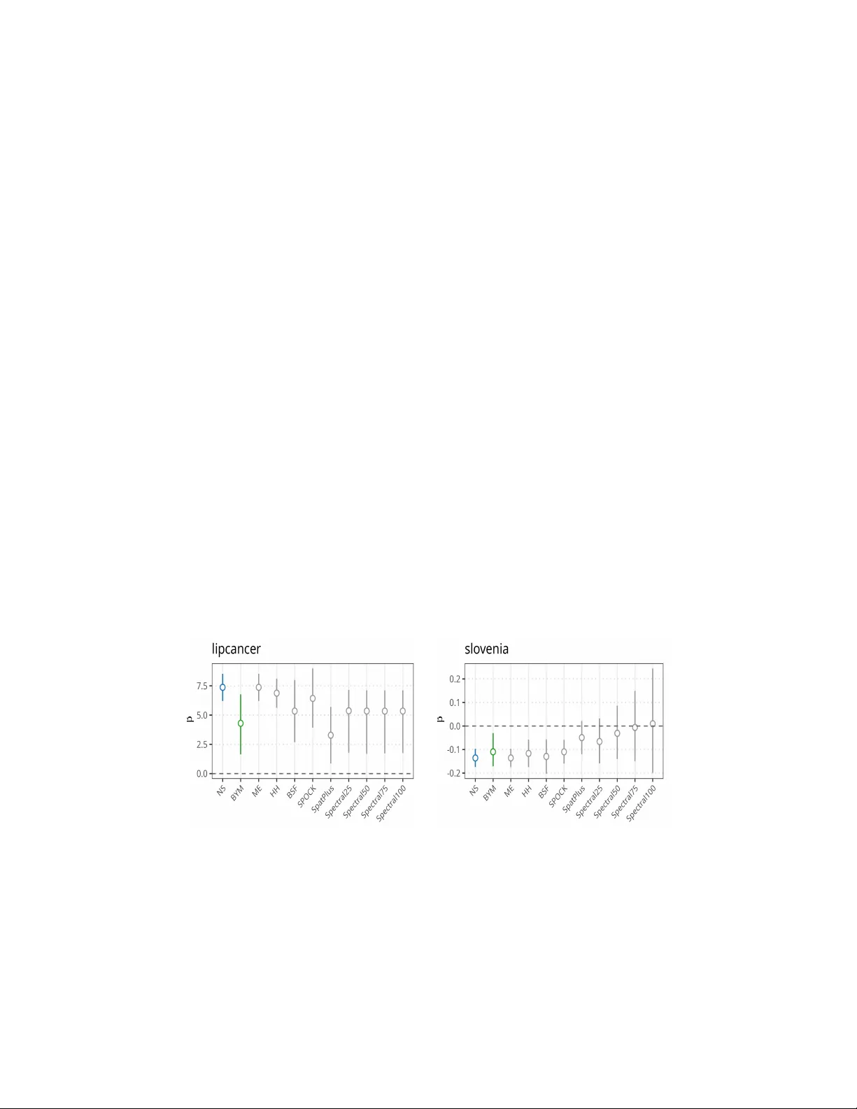
Spatial Confounding: A review of concepts, c hallenges, and curren t approac hes Isaque Vieira Mac hado Pim 1 , Marcos Oliv eira Prates 2 and Luiz Max Carv alho 1 1 Scho ol of A pplie d Mathematics, Getulio V ar gas F oundation, Br azil, e-mail: isaque.pim@fgv.br ; lmax.fgv@gmail.com 2 Dep artment of Statistics, Universidade F eder al de Minas Ger ais, Brazil, e-mail: marcosop@gmail.com Abstract: Spatial confounding is a p ersistent challenge in spatial statis- tics, inﬂuencing the validit y of statistical inference in mo dels that analyze spatially-structured data. The concept has been interpreted in v arious wa ys but is broadly deﬁned as bias in estimates arising from unmeasured spatial v ariation. In this pap er we review deﬁnitions, classical spatial mo dels, and recent metho dological adv ances, including approaches from spatial statis- tics and causal inference. W e provide an uniﬁed view of the many av ailable approaches for areal as well as geostatistical data and discuss their relative merits b oth theoretically and empirically with a head-to-head comparison on real datasets. Finally , we leverage the results of the empirical c ompar- isons to discuss directions for future research. MSC2020 sub ject classiﬁcations : Primary 62H11; secondary 62D20. Keyw ords and phrases: spatial confounding, spatial statistics, causal inference, spatial regression, bias correction. 1. In tro duction Spatially referenced data emerge in many applied areas, including environmen- tal science, ecology and epidemiology . The latter constitutes a ric h set of ap- plications, such as understanding the spread of infectious disease, p oin ting to determinan ts of increased cancer rates, and in vestigating the asso ciation b e- t w een exp osure to ﬁne particles and c hildho o d developmen t ( Elliott et al. , 2000 ; Reic h, Ho dges and Zadnik , 2006 ; P apadogeorgou, Choirat and Zigler , 2019 ). When used to draw conclusions for spatially referenced data, standard regres- sion mo dels can result in spatial dep endence in the residuals and in v alidate the indep endence assumption ( Cressie , 1993 ; Banerjee, Carlin and Gelfand , 2015 ). A common remedy is to include a ﬂexible spatial eﬀect (e.g., Gaussian pro cess, splines, CAR/SAR) so that remaining dep endence is absorbed b y a spatial ef- fect and uncertaint y is b etter calibrated, improving mo del inference ( W aller and Got w ay , 2004 ). Ho w ever, when co v ariates themselv es v ary smo othly o ver space, the spatial random eﬀect can “comp ete” with those co v ariates for the same signal. The 1 2 Pim et al. resulting collinearity mak es it diﬃcult to distinguish co v ariate eﬀects from the laten t spatial ﬁeld; coeﬃcient estimates may be atten uated, their standard errors inﬂated, and sometimes their sign or signiﬁcance can change relative to a non- spatial mo del. This lack of iden tiﬁability betw een ﬁxed eﬀects and the spatial random eﬀect is known as sp atial c onfounding ( Reic h, Hodges and Zadnik , 2006 ). Since its recognition, an active and evolving literature has clariﬁed when spatial confounding arises and is contin ually dev eloping metho ds to mitigate it. Metho ds to alleviate spatial confounding hav e already b een applied to a wide arra y of areas: joint sp ecies mo deling ( Shirota, Gelfand and Banerjee , 2019 ; V an Ee, Iv an and Hooten , 2022 ; Hui, V u and Ho oten , 2024 ); joint mo deling of cancer ( Azeve do, Prates and Bandyopadh ya y , 2021 ); incidence of p o v ert y ( Gar- cía, Quiroz and Prates , 2023 ); prev alence of psychosis ( Congdon , 2024 ); surviv al data ( Azevedo, Prates and Bandyopadh ya y , 2023 ); Student’s abilities and school facilities ( Cefalo, P ollice and Gómez-R ubio , 2025 ; Flores et al. , 2021 ); hurdle mo dels ( P ereira et al. , 2020 ); and group therap y studies ( P addo ck, Leininger and Hunter , 2016 ). Despite a rapidly expanding to olb o x for mitigating spatial confounding, the evidence is fragmented – deﬁnitions, estimands, tuning choices, and performance metrics v ary across studies – so results do not cum ulate and practitioners lack clear guidance ab out which metho d works b est under which conditions. In this pap er, we provide a thorough review of metho ds dedicated to alleviating spatial confounding: for each, we summarize the form ulation, the original con tribu- tions, reference applications to guide practitioners, and curren t implemen ta- tions. W e then place leading approaches on equal fo oting and conduct a large, standardized comparison study across div erse real datasets, harmonizing tar- gets of inference and ev aluation metrics to enable a fair, side-by-side compar- ison. The outcomes are practical scenario-based recommendations that clarify the bias–v ariance trade-oﬀs of comp eting metho ds and help readers choose an appropriate strategy for their data. The remainder of paper is organized as follo ws: In Section 2 , w e presen t the bac kground and notation for spatial confounding. Section 3 reviews early w orks on spatial statistics,exploring spatial ﬁltering methods. Restricted spatial regression (RSR) models are discussed in Section 4 for b oth areal and geostatis- tical data. W e also discuss T ransformed Gaussian Marko v random ﬁelds (TM- GRF) and the consequences of orthogonal smo othing. In Section 5 , the scale of confounding is introduced, along with adjustmen t metho ds such as spatial basis adjustmen t, geoadditive structural equation mo dels (gSEM), the Spatial+ approac h, sp ectral adjustmen t, correlating Gaussian random ﬁelds, and regu- larized spline functions. An analytical framew ork for confounding is dev elop ed in Section 6 and Section 7 presents a persp ective from causal inference, cov- ering topics such as prop ensit y score adjustment, distance-adjusted prop ensit y score matching and double mac hine learning for spatial confounding. Section 8 con tains, to the best of our knowledge, the broadest empirical study of spatial confounding metho ds in the literature. Finally , Section 9 presents conclusions and future directions. Sp atial Confounding: A r eview 3 2. Bac kground and notation Consider a spatial domain D where we observe data at lo cations s ∈ D . This spatial domain can take diﬀerent forms depending on the nature of the data; for instance, in a geostatistical setting D ⊂ R 2 , where eac h lo cation s ∈ D repre- sen ts a coordinate pair in a contin uous space. F or areal data on the other hand, the spatial domain consists of a ﬁnite set of discrete regions, D = { 1 , . . . , n } , where each s corresp onds to a predeﬁned spatial unit such as a count y , city , or coun try . In this framew ork, spatial relationships are often described using adja- cency structures or neighborho o d matrices to capture the spatial dep endencies b et ween regions ( Banerjee, Carlin and Gelfand , 2015 ). W e use W to refer to a spatial weigh t matrix throughout the text. Spatial regression mo dels are commonly used when residual spatial dep en- dence persists after accounting for observed v ariables ( Cressie , 1993 ). This resid- ual dep endence can be attributed to an unobserved spatially structured v ariable ( W aller and Got w a y , 2004 ). This in turn motiv ates the follo wing data-generating pro cess, which underpins v arious metho ds for addressing confounding: Y ( s ) = β 0 + β X X ( s ) + Z ( s ) + ε ( s ) . (1) Here, Y ( s ) represents the outcome v ariable, X ( s ) denotes the exp osure of inter- est, and Z ( s ) captures an unobserved (unmeasured) spatially structured v ari- able. The term ε accounts for random error. The primary goal is to accurately estimate the main eﬀect β X . How ever, since Z ( s ) is unobserv ed, its omission can introduce bias in the estimation of β X . This issue is known as confounding, and when the unobserv ed v ariable Z ( s ) exhibits spatial structure, it is sp eciﬁ- cally referred to as spatial confounding . Metho ds designed to address spatial confounding aim to mitigate the estimation bias in β X , ensuring more reliable inference. F ollo wing the approach of Khan and Berrett ( 2023 ), we diﬀerenti- ate betw een the data-generating model ( 1 ) and the analysis mo dels used for inference. These mo dels are, broadly: Non-Spatial Mo dels : Y ( s ) = β 0 + β N S X X ( s ) + ε ( s ) , (2) Spatial Mo dels : Y ( s ) = β 0 + β S X X ( s ) + γ ( s ) + ε ( s ) , (3) Spatially A djusted Mo dels : ˜ Y ( s ) = β 0 + β AS X ˜ X ( s ) + γ ( s ) + ε ( s ) . (4) Here, ε ( s ) represen ts independent and identically distributed (i.i.d.) noise with v ariance σ 2 , while γ ( s ) represen ts a term commonly included in spatial mo dels to accoun t for spatial dep endence. F or multiv ariate cov ariates, the slop e parameter is vector-v alued, so β X is replaced by β ∈ R p and the linear term is written as X ( s ) ⊤ β . In areal data, γ ( s ) typically represents a spatially struc- tured random eﬀect, often mo deled using spatial linear mixed mo dels suc h as Conditional Autoregressiv e (CAR, Besag , 1974 ) or Simultaneous Autoregressiv e (SAR, Anselin and Bera , 1998 ) mo dels and man y others (e.g., Besag, Y ork and Mollié , 1991 ; Prates, Dey and Lachos , 2012 ; Cruz-Rey es, Assunção and Loschi , 2023 ). These mo dels imp ose spatial correlation based on the neigh b orhoo d struc- ture, ensuring that geographically closer areas exhibit stronger dep endencies. In 4 Pim et al. geostatistical data, γ ( s ) generally represen ts a smo oth spatial surface, making the mo del a partial linear model. Alternatively , it can b e in terpreted as a re- alization of a contin uous Gaussian random ﬁeld, commonly sp eciﬁed using a Matérn cov ariance function. The Matérn ﬁeld provides a ﬂexible framew ork for mo deling spatial correlation, allo wing con trol o ver smo othness, v ariance, and range of spatial dep endence ( Matérn , 2013 ). In the adjusted model, the trans- formed v ariables ˜ Y ( s ) and ˜ X ( s ) diﬀer from the original Y ( s ) and X ( s ) due to the spatial adjustmen t, whic h alters the spatial structure of the input data used in the mo dels. W e now review the currently av ailable literature on spatial confounding, high- ligh ting the adv ances and seeking to ﬁll in the gaps b et w een pap ers in order to pro vide a coherent view of the challenges and promising directions for the area. 3. Early w ork on Spatial Statistics In order to con textualize the main methodological approaches to spatial con- founding, it pays to consider the history of Spatial Statistics as a whole. In a recen t discussion, Donegan ( 2025 ) highlights the parallels b et w een the gro w- ing literature on spatial confounding and the well-established b o dy of work on spatial auto correlation. Despite these historical insigh ts, many classical mo dels from the spatial auto- correlation literature are often ov erlo ok ed when ev aluating methods for address- ing spatial confounding. In particular, key contributions from the econometrics literature are frequently absen t from these discussions. F or instance, LeSage and P ace ( 2009 ) dedicates a section to the study of omitted v ariable bias, illustrat- ing ho w spatial regression mo dels can mitigate this bias more eﬀectively than ordinary least squares (OLS) metho ds. A key metho d in the spatial statistics literature that directly relates to spa- tial confounding is the idea of spatial ﬁltering (SF). SF aims at impro ving the robustness and accuracy of spatial data analysis by decomp osing a spatial v ari- able in to three distinct comp onen ts: a deterministic trend, a spatially structured random comp onent, and random noise ( Griﬃth and Chun , 2014 ). This decom- p osition helps isolate the eﬀects of spatial dep endence, allo wing for more reliable statistical inference. F ormally , the goal is to decomp ose a geographic v ariable Y as Y = Y ∗ ( s ) + ν ( s ) , where ν ( s ) represents the spatially auto correlated comp onen t, and Y ∗ ( s ) is the indep endent (or spatially-ﬁltered) component. The key idea b ehind this decomp osition is to remov e spatial dep endence from Y , ensuring that standard statistical metho ds can b e applied to Y ∗ ( s ) without violating assumptions of indep endence. Spatial ﬁltering techniques include eigenv ector-based metho ds (e.g., eigen- v ector spatial ﬁltering), which construct spatial basis functions from the eigen- decomp osition of a connectivity matrix ( Griﬃth , 2003 ; Griﬃth and Ch un , 2014 ; Tiefelsdorf and Griﬃth , 2007 ). Although F ourier-domain ﬁltering is less com- monly used as an explicit adjustmen t device in spatial regression, frequency- domain methods are standard in digital image pro cessing and remote sensing, Sp atial Confounding: A r eview 5 where manipulating the spatial-frequency sp ectrum is routinely used to sup- press high-frequency (small-scale) noise and remov e perio dic artifacts in im- agery ( Ric hards and Jia , 1999 ; Scho wengerdt , 2007 ; Gonzalez and W o o ds , 2022 ; Whittle , 1954 ). Once the spatial dep endence is accounted for, inference can b e p erformed on Y ∗ using traditional statistical mo dels, such as OLS regression, without concerns of spatial auto correlation distorting results. The Spatial Lag Model (SLM; Anselin and Bera , 1998 ) serves as a founda- tional example of spatial ﬁltering. By mo deling the outcome as Y = ρ W Y + X β + ε , the transformation ( I − ρ W ) Y = X β + ε eﬀectively applies a high-pass ﬁlter to the outcome v ariable. This operation subtracts lo cal means—represented b y the spatially weigh ted av erage W Y —to remo ve spatial trends and isolate the non-spatial comp onent of Y for inference on β ( Pace and LeSage , 2008 ). F ailing to account for this dep endence can lead to severe omitted v ariable bias in OLS estimates, particularly when spatial auto correlation exists across regressors and disturbances ( Pace and LeSage , 2008 ). This bias often leads to incorrect em- pirical conclusions; for instance, SLM corrections hav e b een shown to rev erse coun ter-in tuitive OLS results in environmen tal hedonic pricing ( Brasington and Hite , 2005 ) and retail sales modeling ( Lee and P ace , 2005 ), yielding estimates that align more closely with economic theory . 3.1. Sp atial ﬁltering metho ds Mo ving on to key spatial ﬁltering methods, tw o approac hes are presented in Getis and Griﬃth ( 2002 ). The ﬁrst metho d inv olves a direct transformation of the v ariable using its Local Indicator of Spatial Asso ciation (LISA, Anselin , 1995 ), sp eciﬁcally the Getis-Ord G i ( d ) statistic ( Getis , 1991 ). The Getis-Ord statistic measures the lo cal spatial auto correlation of a v ariable at a given lo- cation i by assessing the concentration of high or lo w v alues within a speciﬁed distance d . F ormally , G i ( d ) is giv en by: G i ( d ) = P j w ij ( d ) x j P j x j , where x j = X ( s j ) is the v alue of the v ariable at lo cation s j , w ij ( d ) is a spatial w eigh t that deﬁnes the neigh b oring structure within distance d . In the case of a binary adjacency matrix W for areal data, w ij = ( W ) ij that is 1 if the areas are neigh bors and 0 otherwise. The denominator ensures normalization based on the sum of all observ ations. This expression is the observe d v alue of the statistic for lo cation i . The exp e cte d v alue of the statistic for lo cation i is of the form W i / ( n − 1) , where W i is the sum of binary w eights in row i . The ﬁltering transformation of the observ ed data v al- ues X ( s i ) = x i applied is then: x ∗ i = x i Expected i Observed i , i.e. x ∗ i = x i  W i n − 1  /G i ( d ) . The second spatial ﬁltering method , in tro duced b y Griﬃth, is known as eigen v ector spatial ﬁltering (ESF) or Moran eigenv ector ﬁltering. This approac h lev erages the computational formula for Moran’s I statistic ( Moran , 1950 ) to decomp ose spatial auto correlation in to orthogonal and uncorrelated spatial com- p onen ts. Moran’s I measures global spatial autocorrelation, capturing the degree to which nearby v alues of a v ariable are similar. The ESF metho d decomp oses Moran’s I statistic into spatial eigen vectors, whic h represent uncorrelated spatial 6 Pim et al. patterns. These eigenv ectors serve as laten t v ariables that capture systematic spatial dep endence in the dataset. The eigenv ectors used for spatial ﬁltering are derived from a mo diﬁed spatial w eigh ts matrix W ∗ , which appears in the numerator of the Moran co eﬃcien t ( Griﬃth, Chun and Li , 2019 ): W ∗ = M W M , where M = I − 11 T n . (5) Here W is the spatial w eights matrix deﬁning the spatial relationship among observ ations, I is the identit y matrix, 1 is a v ector of ones, M is a cen tering matrix that ensures the eigenv ectors capture spatial v ariations while remo ving non-spatial trends. Once the eigenv ectors are extracted from the transformed matrix M W M , they represent a set of indep enden t spatial patterns present in the data. The next step is to select a subset of eigenv ectors based on their Moran’s I v alues. T ypi- cally , eigen vectors exceeding a certain Moran’s I threshold are c hosen to account for signiﬁcant spatial dep endence ( Hughes and Haran , 2013 ). Once a subset of eigen v ectors are selected, they are regressed against the dep enden t v ariable Y in a step wise fashion under a multiple regression mo del: Y = P m k =1 α k E k + ε , where E k are the selected spatial eigenv ectors, and α k are their correspond- ing regression co eﬃcien ts. The residuals of this regression correspond to the spatially ﬁltered version of Y , which are largely free of spatial auto correlation, Y ∗ ( s ) = Y − P m k =1 α k e k . Th us, the ﬁltered v ariable Y ∗ ( s ) can b e used in traditional statistical mo dels without violating the assumption of indep endence. F or more details, see Griﬃth ( 2003 ) and Griﬃth, Chun and Li ( 2019 ). A Bay esian formulation for the spatial ﬁlter was prop osed by Hughes ( 2017 ) and b y Donegan, Chun and Hughes ( 2020 ). The structure is the same as in the Moran eigen vector ﬁltering, where Hughes ( 2017 ) formulates Bay esian eigen v ector ﬁltering by augmen ting the regression with a selected subset of Moran eigen vectors and assigning spherical priors to the corresponding co eﬃcien ts, whereas Donegan, Chun and Hughes ( 2020 ) re- tains the full eigenv ector basis but places regularizing shrinkage priors on the co eﬃcien ts to control complexit y . The key adv an tage of Donegan’s approach is that it replaces ad ho c eigen v ector selection with principled regularization and mo del av eraging, propagating uncertaint y about the spatial ﬁlter into inference for the co eﬃcien ts. 4. Restricted Spatial Regressions Signiﬁcan t atten tion has b een directed tow ard the bias that arises when incor- p orating spatial smo othing in to regression frameworks in the disease mapping literature. A seminal example is pro vided by Clayton, Bernardinelli and Mon- tomoli ( 1993 ), who analyzed lung cancer incidence in Sardinia and describ ed this phenomenon as "confounding by lo cation". Building on these observ ations, Reic h, Ho dges and Zadnik ( 2006 ) reasoned on this issue, framing it as a form of Sp atial Confounding: A r eview 7 collinearit y where the spatial random eﬀects comp ete with the cov ariate matrix X to explain the same v ariation. T o mitigate this, they prop osed Restricted Spatial Regression (RSR), which constrains the spatial random eﬀects to the orthogonal complement of the column space of X . This restriction ensures the spatial comp onen t captures only residual geographic structure, prev enting it from attenuating or destabilizing inference on the regression coeﬃcients. The w ork b y Reich, Ho dges and Zadnik ( 2006 ) prov ed foundational, motiv ating a recen t spur in the spatial confounding literature. In the follo wing section, w e de- tail the core mo dels of the RSR literature, highlighting their resp ectiv e strengths and inferential trade-oﬀs. W e ﬁrst examine the foundational RSR framework for areal data, follow ed by its extension to con tin uous spatial pro cesses. Finally , we discuss recent critiques of RSR, sp eciﬁcally addressing how the orthogonal con- strain t may lead to under co v erage of uncertaint y interv als. 4.1. R estricte d Sp atial R e gr essions on ar e al data Reic h, Ho dges and Zadnik ( 2006 ) tak e a Bay esian approac h to the study of the impact of an ICAR prior on the estimation of β X . The authors employ the ICAR mo del as a spatial comp onent in the following formulation: Y | β , γ , τ ϵ ∼ N ( X β + γ , τ ϵ I ) , with γ | τ γ ∼ N ( 0 , τ γ Q ) , where γ is the ICAR spatial eﬀect, Q is the precision matrix for the ICAR, τ ϵ and τ γ are precision hyperparameters related to the Gaussian observ ations and the ICAR, resp ectiv ely . In the case of spatial linear regression, it is possible to analytically calculate the marginal mean integrating out the laten t eﬀect as: E ( β | τ ϵ , τ γ , Y ) = ( X T X ) − 1 X T ( Y − ˆ γ ) = β N S X − ( X T X ) − 1 X T ˆ γ . F rom the result ab ov e it is possible to see that spatial models diﬀer in estimation from traditional linear models by a quantit y inv olving the laten t eﬀect. If one could make the latent eﬀect orthogonal to the design matrix, the bias term in v olving the laten t eﬀect w ould v anish. T o ac hiev e this, Reich, Hodges and Zadnik ( 2006 ) prop ose the follo wing mo del sp eciﬁcation, henceforth called the RHZ mo del. First, deﬁne the pro jection matrix onto the column space of X , P X = X T ( X T X ) − 1 X , and P ⊥ X = I − P X its orthogonal complemen t. The structured random eﬀect can b e decomp osed into a comp onen t on the span of X , and a comp onen t orthogonal to the span of X b y taking γ = γ X + γ ⊥ = K γ 1 + L γ 2 . The proposed solution is to set γ 1 to zero, neutralizing the comp onen ts of the random eﬀect in the span of X . The RHZ mo del is then form ulated as Y = X β X + L γ 2 + ε, p ( γ 2 | τ s ) ∝ τ κ s exp  − τ s 2 γ T 2 L T QL γ 2  . This approach oﬀers a more computationally eﬃcient solution by utilizing L T , a ( n − p ) × n matrix, rather than P ⊥ , which is an n × n matrix. Ho w ever, 8 Pim et al. since the n umber of cov ariates p is typically muc h smaller than the n umber of areas n , this reduction do es not yield a substantial computational adv antage. A b etter computational relief came with the w ork of Hughes and Haran ( 2013 ), who noticed that the RHZ model is computationally ineﬃcient and that the mo del accounts for b oth p ositiv e and negative spatial auto correlation, arguing that the latter is not desired in spatial applications. One of the reasons for the ineﬃciency is that the precision matrix pro duced by the pro jections used b y Reich, Ho dges and Zadnik ( 2006 ) is not sparse. In addition, negative spatial correlation arises from the fact that in the construction of L , the underlying graph is not accoun ted for. T o address this, Hughes and Haran ( 2013 ) deﬁne the Moran operator P ⊥ X W P ⊥ X and replace L b y a matrix M q comp osed of eigen v ectors of the Moran op erator. Notice ho w this resembles the modiﬁed spatial weigh t matrix in Equation ( 5 ). They show ed that the Moran op erator retains the spatial patterns of the data better than the columns of L and it is only necessary to select the h ≪ n higher positive eigenv alues of the sp ectrum of the Moran operator, called attractive eigen v alues, reducing computational burden. Another ma jor improv ement in the computational p erformance for RSR mod- els w as developed by Prates, Assunção and Rodrigues ( 2019 ). Ev en though Hughes and Haran ( 2013 ) attempt to impro ve computational eﬃciency by re- ducing the dimension of the problem, muc h of the eﬀectiveness of ICAR mo dels is that the random ﬁelds are very sparse. This allows for fast sparse matrix rou- tines to b e used ( Rue and Held , 2005 ). Prates, Assunção and Ro drigues ( 2019 ) try to alleviate confounding b y preserving muc h of the structure and the rou- tines used to ﬁt ICAR mo dels b y pro jecting the graph deﬁned b y the study area onto the orthogonal space of the design matrix X , a metho d they dubb ed SPOCK (SP atial Orthogonal Centroid “K”orrection.). With the pro jected v er- tices in hand, they construct a sparse precision matrix Q ⊥ for analysis. The ﬁrst step is to calculate the new set of cen troids c ∗ b y pro jecting c on to the orthogonal space of X , that is, using the projection matrix P c X . After the new set of centroids is pro duced, a new adjacency matrix can b e pro duced by ﬁnd- ing the k -nearest-neigh b ors of eac h centroid, picking k for eac h region as the n um b er of neighbors it originally had. By doing this, the sparsity of the original adjacency matrix will b e kept, thus maintaining the eﬃciency of sparse meth- o ds. SPOCK can also b e applied in a multiv ariate con text ( Azevedo, Prates and Bandy opadh ya y , 2021 ). Another k ey asp ect explored in their work is the T yp e-S error rate in RSR mo dels for areal data, following the approac h of Hanks et al. ( 2015 ). They deﬁne a Type-S error as occurring when a regression parameter is truly zero ( β X = 0 or β ∗ X = 0 ), yet its 95% symmetric p osterior credible interv al does not con tain zero (see also Gelman and Carlin ( 2014 )). Their ﬁndings reveal an elev ated Type- S error rate in RSR mo dels, further reinforcing criticism of their reliability in spatial analyses. Nobre, Schmidt and Pereira ( 2021 ) examine spatial confounding in multilev el mo dels with clustered observ ations, showing that bias in ﬁxed eﬀects p ersists ev en with indep endent random intercepts due to within-cluster dep endencies. Sp atial Confounding: A r eview 9 They extend RSR to hierarc hical settings, concluding that while RSR reduces bias for cluster-lev el eﬀects it increases Type-S error rates and may worsen estimation of unit-level co eﬃcien ts when predictors are correlated. Their sim- ulations reveal that the magnitude of the bias dep ends on the spatial scales of co v ariates and random eﬀects, in agreement with previous work by Paciorek ( 2010 ) and Page et al. ( 2017 ) and which are reviewed in Section 5 . Hui and Bondell ( 2022 ) studies spatial confounding in the context of Generalized Esti- mating Equations (GEE) and ﬁnd that spatial confounding can also arise in the setting of GEE and prop ose a restricted spatial w orking correlation matrix to correct for confounding. 4.2. R estricte d Sp atial R e gr essions on Ge ostatistic al data Hanks et al. ( 2015 ) bring the discussion of spatial confounding to geostatistical data and extend the metho ds presented b y Reich, Ho dges and Zadnik ( 2006 ) and Hughes and Haran ( 2013 ) to data with contin uous supp ort. T o this end, the authors mo v e from a ICAR mo del speciﬁcation to a Matérn sp eciﬁcation to mo del auto correlation. That is, the mo del now follo ws Y ( s ) = X ( s ) β X + γ + ε , γ ∼ N ( 0 , Σ ) , with Σ ij = σ 2 C ν ( d ij ; ϕ ) = σ 2 1 Γ( ν )2 ν − 1  √ 2 ν d ij ϕ  ν K ν  √ 2 ν d ij ϕ  , (6) where d ij is the Euclidean distance b et ween the spatial locations of the i - th and j -th observ ations, σ 2 is the partial sill parameter, ν is the Matérn smo othness parameter, ϕ is a range parameter, and K ν ( · ) is the modiﬁed Bessel function of the second kind (e.g, Cressie , 1993 ). T o p erform RSR in a eﬃ- cien t wa y , they propose a metho d to constrain γ b y “conditioning by Kriging” ( R ue and Held , 2005 ). The orthogonalization is p erformed ad ho c during the MCMC sampling pro cess, by sampling from the Matérn ﬁeld γ ∼ N ( µ , Σ ) with the constraint X T γ = 0 . This can be accomplished by the transformation: γ ∗ ∼ N ( µ , Σ ) , and γ = γ ∗ − ΣX ( X T ΣX ) − 1 X T γ . Hanks et al. ( 2015 ) also con- tributes to the study of Type-S errors in RSR. They ﬁnd through sim ulations that Type-S errors increase as spatial range (correlation distance) increases and RSR p erforms po orly when the true model is a SGLMM. Another exploration of the same scenarios describ ed by Hanks et al. ( 2015 ) is done by Heﬂey et al. ( 2017 ). They do not use RSR, but rather explore regularized mo dels with con- founded data adapting the priors for co eﬃcien ts to include regularization. They sho w empirically that regularization reduces problems with multicollinearit y and impro v es Marko v c hain Monte Carlo (MCMC) mixing. Chiou, Y ang and Chen ( 2019 ) argue that RSR metho ds hav e b een developed primarily within a Ba y esian framework. Their contribution to the literature is to extend RSR to the frequentist setting b y formulating estimators based on an adjusted version of the generalized least squares (GLS) estimator. More recen tly , 10 Pim et al. Chiou and Chen ( 2025 ) connect RSR’s pro jection idea to low-rank geostatistical mo deling via Fixed Rank Kriging (FRK): they use an FRK representation of the laten t spatial pro cess to estimate the comp onen t aligned with the cov ariate space and then correct inference on β X for spatial confounding. In this sense, FRK serves as a practical implemen tation lay er for the same spatial-confounding mec hanism that motiv ates RSR, without relying solely on a hard orthogonalit y constrain t. 4.3. T r ansforme d Gaussian Markov R andom Fields Although not strictly an RSR metho d, transformed Gaussian Marko v Random Fields (TGMRF, Prates et al. , 2015 ) mitigate confounding by structurally iso- lating the marginal mean sp eciﬁcation from the spatial dep endence. While a standard spatial GLMM induces dependence via an additive laten t term in the link function (i.e., g ( µ i ) = x i β + ε i ), the TGMRF framework models the random mean v ector µ directly via a Gaussian copula. A random ﬁeld is de- noted µ ∼ TGMRF n ( F β , Q ρ ) if it couples indep endent marginal distributions F = ( F 1 , . . . , F n ) with a latent GMRF dep endence structure characterized b y precision matrix Q ρ . The resulting hierarchical formulation is: y i | µ i ∼ π ( y i | µ i ) , µ ∼ TGMRF n ( F β , ν , Q ρ ) . Here, the regression co eﬃcien ts β solely parameterize the marginals F , while the spatial decay ρ is restricted to the copula. The authors argue that this orthogonalit y prev ents the dependence structure from in terfering with the marginal mo dels, eﬀectiv ely alleviating confounding. Prates et al. ( 2021 ) formalized this capability , reporting that TGMRF s oﬀer a compromise b et w een standard SGLMMs and RSR metho ds. They reduce v ariance inﬂation under strong confounding while retaining b etter type-I er- ror control and interv al cov erage than restricted approaches, which can become o v erconﬁdent when confounding is absent. A spatio-temporal extension of this framew ork was prop osed by Prates et al. ( 2022 ). 4.4. Conse quenc es of ortho gonal pr oje ction of sp atial eﬀe cts RSR dominated the spatial confounding literature for more than a decade, but has since b een argued to be problematic. Khan and Calder ( 2022 ) and Zim- merman and Hoef ( 2022 ) w ere the ﬁrst to point out the inconsistencies of the RSR metho ds and argue against the use of RSR. Most of the mo dern accoun ts already accept these conclusions and reinforce them ( Urdangarin, Goicoa and Ugarte , 2023 ; Dup ont, Marques and Kneib , 2023 ; Khan and Berrett , 2023 ; Done- gan , 2025 ). Even when assuming a data-generating mechanism that agrees with RSR, co v erage of the true parameters is worse than a NS mo del. This can b e c hec ked either with Ba yesian methods by means of simulation and analysis of T yp e-S error as done by Khan and Calder ( 2022 ) or by a frequentist theoretical analysis of the bias of RSR estimators as done by Zimmerman and Ho ef ( 2022 ). Sp atial Confounding: A r eview 11 On the Ba yesian side, Prates, Assunção and Ro drigues ( 2019 ), Hanks et al. ( 2015 ) and Khan and Calder ( 2022 ) study the Type-S error for RSR mo dels. They all rep orted higher rates of Type-S error for RSR mo dels in all p ossible scenarios. Khan and Calder ( 2022 ) brings an analytical explanation for the el- ev ated error rates, where they claim that RSR metho ds will only capture the regression co eﬃcient if the non-spatial mo del do es. F urthermore, RSR metho ds will alw a ys hav e higher rates of Type-S error than the non-spatial mo del, ev en if there is no spatial confounding. Ho w ever, Bradley ( 2024 ) argues that these sub-optimal inferential prop erties arise from a sp eciﬁc interpretation that incor- rectly assumes equiv alence b et w een confounded and deconfounded eﬀects, and demonstrates that spatial deconfounding remains a reasonable statistical prac- tice when viewed as a reparameterization that pro duces inferences equiv alent to the standard spatial linear mixed mo del. On the frequen tist side, Zimmerman and Ho ef ( 2022 ) claimed that decon- founding a spatial linear mo del by orthogonalization is “bad statistical prac- tice and should b e a voided” . They come to this conclusion b y studying the prop erties of the MLE estimators of models ( 2 ), ( 3 ), and ( 4 ). When Equa- tion ( 4 ) for RSR models is specialized to a frequen tist setting we get Y = X ( s ) β X + P c X γ ( s ) + ε ( s ) . Thus, assuming the structured comp onent γ ( s ) has v ariance σ 2 G , the marginal cov ariance matrix of Y is given b y Σ RS R = σ 2 [( I − P X ) G ( I − P X ) + I ] . Then the empirical GLS estimator for the RSR mo del is ˆ β RS R =  X T ˆ Σ − 1 RSM X  − 1 X T ˆ Σ − 1 RSM Y . They also consider based on Hughes and Haran ( 2013 ), estimators deriv ed from the Moran operator. The marginal co v ariance matrix of Y is giv en b y Σ M oran = σ 2 h M q M T q G M q M T q + I i . Then the empirical GLS estimator for the β is ˆ β M oran =  X T ˆ Σ − 1 Moran X  − 1 X T ˆ Σ − 1 Moran Y . More generally deconfounded estimators can b e pro duced by transforming the structured random eﬀect using an y matrix deriv ed from the column space of P c X . Based on these estimators, they show that the CIs for RSR models are narro w er than the the standard CIs from NS mo dels. This is in contradiction with a pragmatic thinking in spatial statistics, as describ ed b y Donegan ( 2025 ), that each observ ation in a spatial context is not as informativ e as an independent sample. So any uncertaint y quantiﬁ cation that takes this into accoun t should pro duce wider interv als. F ortunately for RSR, Zimmerman and Ho ef ( 2022 ) ﬁnd that despite its inferiorit y in estimating ﬁxed eﬀects, RSR do es not signiﬁcan tly degrade spatial prediction. The b est linear unbiased predictor (BLUP) of new spatial observ ations remains identical under b oth the original spatial mo del and the deconfounded mo del. RSR metho ds play ed a crucial role in reigniting discussions on fundamen tal c hallenges in spatial regression but hav e since pro ven problematic. The literature 12 Pim et al. mo v ed on to new mo dels, but key ﬁndings are still present in many of the w orks in the area. 5. Scale of Confusion While RSR metho ds fo cus on mo del reformulation, Paciorek ( 2010 ) introduced the "scale of confounding" to explain how spatial structure dictates bias from a data-generation persp ective. Under the framew ork of Equation ( 1 ), consider an exp osure X and unmeasured confounder Z modeled as Gaussian pro cesses: X ∼ N ( 0 , σ 2 x R ( θ x )) and Z ∼ N ( 0 , σ 2 z R ( θ z )) , with Co v ( X , Z ) = ρσ x σ z R ( θ c ) . P aciorek ( 2010 ) demonstrated that standard spatial regression (kriging or GLS) do es not inherently eliminate bias. Speciﬁcally , the induced bias in the GLS estimator, E ( ˆ β x − β x | X ) = ρ σ z σ x β z , is identical to that of OLS. Ho wev er, by adopting a multiscale decomp osition X = X c + X u , where X c shares a spatial range with Z , the bias b ecomes scale-dependent: E ( ˆ β X | X ) = β x + c ( X ) ρ σ z σ c β z . Here, the function c ( X ) incorp orates the in terpla y b etw een spatial scales. This rev eals that spatial mo deling can actually exacerbate bias if the confounded spatial range is shorter than the unconfounded range; mitigation only o ccurs when the confounded range is the broader of the tw o. This foundational insight underscores that the eﬀectiveness of spatial adjustment depends entirely on the relativ e scales of the exp osure and the unmeasured confounder. P age et al. ( 2017 ) further studied the importance of scale for estimation of the parameters but also addresses prediction. Narcisi, Greco and T rivisano ( 2024 ) pro vides a analysis of confounding through the lens of quadratic forms. This concept has already b een explored in confounding adjustment metho ds for time series ( Dominici, McDermott and Hastie , 2004 ; Szpiro et al. , 2014 ). When the exp osure of in terest v aries at ﬁne spatial scales, smo othing the se- ries can help isolate this v ariation for inference. This approach also aligns with the ﬁltering metho ds discussed in Section 3 , which remov e large-scale spatial v ariation to facilitate inference using the smo othed v ariables. F ollo wing the dev elopments of P aciorek ( 2010 ) another line of methodology w as developed, fo cusing on adjusting for spatial information in the exp osure, or taking into account a joint mec hanism b ehind the generation of the exp osure. 5.1. Sp atial Basis A djustment and R e gularization T o address spatial confounding in cohort settings, Keller and Szpiro ( 2020 ) pro- p ose decomp osing the exp osure, cov ariates, and error term in to smo oth spatial surfaces via hierarc hical basis functions { h 1 , h 2 , . . . } (e.g., splines, F ourier, or w a velets) ordered by increasing resolution. Let H m denote the ﬁrst m basis functions. They introduce tw o adjustment strategies: (i) directly including H m as cov ariates in a semiparametric regression, or (ii) a spatial ﬁltering approach where the exp osure X is pro jected onto the space orthogonal to H m . By utilizing bases ordered by resolution, these metho ds isolate the ﬁne-scale v ariation of the Sp atial Confounding: A r eview 13 exp osure for inference while remo ving the large-scale spatial comp onen ts typi- cally asso ciated with unmeasured confounders. A key contribution of Keller and Szpiro ( 2020 ) is pro viding a formal mechanism for identifying the appropriate spatial scale for confounding adjustment. Because the bias and v ariance of the exp osure eﬀect are highly sensitive to the num b er of basis functions used, the authors developed criteria to estimate the "optimal" scale m for diﬀerent basis t yp es. By ev aluating the trade-oﬀ b et ween bias reduction (achiev ed by including more bases) and loss of eﬃciency (caused b y removing to o muc h exp osure v aria- tion), their framew ork allows researchers to ob jectiv ely determine the resolution at which the exp osure pro vides the most reliable signal for inference. While Keller and Szpiro ( 2020 ) approac h often requires pre-selecting this n um b er of bases m via cross-v alidation or information criteria, Zaccardi et al. ( 2025 ) introduce a Ba yesian semiparametric mo del that automates scale selec- tion through regularization. They approximate the unobserved spatial factor using principal spline basis functions B and emplo y spik e-and-slab priors to iden tify the most critical bases: β s j | γ j ∼ γ j N (0 , ψ 2 j ) + (1 − γ j ) N (0 , c 0 ψ 2 j ) . Here, the indicator γ j ∼ Bernoulli ( w ) determines basis inclusion, while a small c 0 en- courages sparsit y . This regularized framework—whic h can be implemented with v arious prior v ariances suc h as the pro duct moment (pMOM) prior ( Johnson and Rossell , 2012 )—provides a data-driven mec hanism to select the appropri- ate spatial resolution for confounding adjustment without manual tuning of the basis rank. 5.2. Sp atial+ Spatial+ ( Dup on t, W o o d and Augustin , 2022 ) is a tw o-stage approac h to spatial confounding that targets the spatial structure of the exp osure rather than al- tering the spatial eﬀect in the outcome mo del. It ﬁrst decomp oses the cov ariate in to spatial and non-spatial comp onents and then p erforms inference using the non-spatial remainder, while retaining a ﬂexible spatial term in the resp onse mo del. One again, let X ( s ) b eing the cov ariate and f ( s ) a smo oth function of space that captures the spatial eﬀect. Spatial+ then decomposes X i in to a spatially dep enden t comp onent f x ( s i ) and residuals r x i : x i = f x ( s i ) + r x i . The mo del then replaces X i with r x i in the spatial analysis mo del, resulting in: Y i = β r x i + f + ( s i ) + ϵ i , where f + ( s i ) is also assumed to b e a smo oth surface that combines the spatial eﬀects f ( s i ) and β f x ( s i ) . This adjustment reduces the collinearity b et ween X i and f ( s i ) , allowing for an unbiased estimation of β . The metho d is straightforw ard to implement using existing regression to ols like thin plate splines. Another adv antage of spatial+ is that all spatial information is retained in the mo del. Many subsequen t mo dels developed from the Spatial+. The Geoadditive Structural Equation Mo del (gSEM), introduced by Thaden and Kneib ( 2018 ), is a direct predecessor to Spatial+ designed to rectify bias from unmeasured spatial confounding. When a shared spatial process aﬀects b oth a co v ariate X ( s ) and the resp onse Y ( s ) , standard geoadditive models ma y 14 Pim et al. misattribute spatial v ariation to the cov ariate. gSEM addresses this b y sepa- rately estimating spatial comp onen ts for X ( s ) and Y ( s ) within a structural equation framew ork, thereby isolating the direct cov ariate eﬀect β x from indi- rect spatial pathw ays. The mo del is speciﬁed with tw o equations: X i = P k z ki γ 1 k + ε 1 i and Y i = X i β x + P k z ki γ 2 k + ε 2 i , where γ 1 k and γ 2 k represen t distinct spatial eﬀects. By explicitly modeling the separate spatial dep endencies, gSEM pro vides a founda- tional approach for bias adjustment that Spatial+ later reﬁnes and simpliﬁes. Marques and Wiemann ( 2023 ) dev elop ed the Ba yesian Spatial+ based on a join t mo del p erspective. The authors argue that adjusting for confounding in tw o stages using frequen tist estimators neglects uncertain ty propagation b et ween stages. They integrate the tw o stages into a joint Bay esian framew ork, allowing uncertain t y propagation and direct parameter inference. They also in tro duce join t priors to restrict spatial smo othness, ensuring unobserved eﬀects do not op erate at ﬁner spatial scales than observed co v ariates. In the original formulation ( Dup on t, W oo d and A ugustin , 2022 ) there is no in- dication on how to conduct prop er uncertaint y quantiﬁcation, but the Bay esian form ulation mak es the task straightforw ard. Urdangarin et al. ( 2024 ) prop osed a simpliﬁed version of Spatial+ for areal data, which instead of ﬁtting a thin plate spline, ﬁlters the co v ariate X ( s ) by remo ving low-frequency eigen v alues. They also extend the metho d to a multiv ariate resp onse scenario. Dup ont and Au- gustin ( 2024 ) extend their metho d to non-linear cov ariate eﬀects. They ac hiev e this by using generalized additiv e models (GAMs, Hastie and Tibshirani ( 1986 )) to mo del the spatial eﬀect, decomposing eac h elemen t of the basis used into a spatial and residual comp onents, and using the residuals as a new basis. 5.3. Sp e ctr al A djustment Motiv ated b y the idea that spatial confounding can b e scale-dep endent, Guan et al. ( 2022 ) recast the problem in the sp ectral domain and develop an adjust- men t that targets confounding at sp eciﬁc spatial frequencies. They assume data coming from a con tinuous spatial domain and the same DGM as in Equation ( 1 ). Both pro cesses X ( s ) and Z ( s ) hav e zero mean and are stationary , and thus hav e sp ectral represen tations X ( s ) = R e iω ⊤ s X ( ω ) dω , z ( s ) = R e iω ⊤ s Z ( ω ) dω , where ω ∈ R 2 is a frequency . The sp ectral pro cesses X ( ω ) and Z ( ω ) are Gaussian with E ( X ( ω )) = E ( Z ( ω )) = 0 and are indep enden t across frequencies, so that for an y ω  = ω ′ , Cov {Z ( ω ) , Z ( ω ′ ) } = Co v {X ( ω ) , X ( ω ′ ) } = Co v {X ( ω ) , Z ( ω ′ ) } = 0 . A t the same frequency , the cov ariance has joint form Co v  X ( ω ) Z ( ω )  =  σ 2 x f x ( ω ) ρσ x σ z f xz ( ω ) ρσ x σ z f xz ( ω ) σ 2 z f z ( ω )  , where σ 2 x and σ 2 z are v ariance parameters, f x ( ω ) > 0 and f z ( ω ) > 0 are sp ectral densities that determine the marginal spatial correlation of x ( s ) and z ( s ) , resp ectiv ely , and the cross-sp ectral densit y f xz ( ω ) determines the de- p endence b et ween the sp ectral pro cesses at diﬀerent frequencies. The condi- tional distribution of Y ( ω ) giv en X ( ω ) , marginalizing ov er Z ( ω ) , is Y ( ω ) | Sp atial Confounding: A r eview 15 X ( ω ) indep ∼ N  β x X ( ω ) + β z α ( ω ) X ( ω ) , τ 2 ( ω ) + σ 2  , where α ( ω ) = ρσ z f xz ( ω ) σ x f x ( ω ) = σ z √ f z ( ω ) σ x √ f X ( ω ) γ ( ω ) , τ 2 ( ω ) = β 2 z σ 2 z f z ( ω ) h 1 − ρ 2 f xz ( ω ) 2 f x ( ω ) f z ( ω ) i . The regression coeﬃcient for X ( ω ) is β ( ω ) = β x + β z α ( ω )  = β x . The addi- tional term b Z ( ω ) = E [ Z ( ω ) | X ( ω )] = α ( ω ) X ( ω ) is the result of attributing the eﬀect of the unmeasured confounder to the resp onse to the treatment v ariable, whic h could induce bias in estimating β x . It is then clear that assumptions ab out the nature of α ( ω ) are necessary to correct for confounding. The authors prop ose tw o approac hes for the correct iden tiﬁcation of the eﬀect β x : unconfoundedness at high frequencies, that is, if w e assume that α ( ω ) → 0 for large ∥ ω ∥ , then E ( Y ( ω ) | X ( ω )) ≈ β x X ( ω ) , and th us β x is identiﬁed; a parsimonious and parametric mo del with constraints on the parameters. This in turn implies that the correlations b etw een X and Z are constan t b etw een all frequencies. It is possible to verify that with this parsimonious sp eciﬁcation, all parameters are identiﬁable. Returning to the spatial domain, the adjustment for confounding is then done b y adjusting the following mo del Y ( s ) | X ( s ) , s ∈ D = β 0 + β x X ( s ) + β z b Z ( s ) + δ ( s ) , b Z ( s ) = Z exp( iω T s ) b Z ( ω ) dω = Z exp( iω T s ) α ( ω ) X ( ω ) dω . Using ˆ Z as a cov ariate can alleviate confounding in some smoothing conﬁg- urations, as describ ed by the authors. T o pro duce ˆ Z , a parsimonious biv ariate Matérn mo del can be assigned to X and Z . The other prop osal of the authors is to ﬁt a semi-parametric mo del by using B-splines to mo del α ( ω ) . In a more recent contribution, Prim et al. ( 2025 ) extend sp ectral metho ds to handle m ultiple exp osures and multiple outcomes simultaneously . They mo del m ultiscale eﬀects using a three-wa y tensor (exp osures x outcomes x spatial scales), applying canonical p oly adic decomp osition to the tensor to induce low- rank structures and enable parameter sharing across exp osures and outcomes. They implemen t it by Bay esian tensor regression using horseshoe priors ( Car- v alho, Polson and Scott , 2010 ) to promote sparsity and preven t o v erﬁtting. 5.4. Corr elating Gaussian R andom Fields Marques, Kneib and Klein ( 2022 ) also construct a metho d inspired by the joint mec hanism generating observ ed and unobserved quantities. They prop ose a joint Gaussian distribution for X ( s ) and Z ( s ) . The authors hypothesize that explic- itly correlating Gaussian random ﬁelds for X ( s ) and Z ( s ) in spatial regression mo dels can reduce bias in regression co eﬃcien t estimates caused b y spatial con- founding. Sp eciﬁcally , b y join tly mo deling the spatial random eﬀect and the co v ariates using a m ultiv ariate Gaussian random ﬁeld, the prop osed mo del aims to better account for the spatial dep endencies and reduce confounding. Let Z ∼ N ( 0 , Σ z ) . They assume that Z ( s ) and X ( s ) are join tly Gaussian distributed 16 Pim et al. suc h that  γ Z  ∼ N  0 µ z  , Σ γ ρ Σ 1 / 2 γ ( Σ 1 / 2 z ) T ρ Σ 1 / 2 z ( Σ 1 / 2 γ ) T Σ z !! . In this setup, all conditional distributions can b e easily calculated, allowing us to calculate the distribution of the spatial eﬀect conditional on the observ ations. F or the parameter ρ , a Penalized Complexity (PC) priors are used. PC priors to the correlation parameter can provide a computationally eﬃcien t w ay to shrink to ward a non-confounded base mo del. That is, the mo del allo ws non- zero ρ only if the data strongly supp orts it, ensuring that spatial confounding is addressed dynamically . The prior takes the form p ( ρ ) = c − 1 2  1 1 − ρ − 1 1 + ( c − 1) ρ  λ p − lR ( ρ ) exp( − λ p − lR ( ρ )) , where l R ( ρ ) = log ( R ( ρ )) and R ( ρ ) = (1 + ( c − 1) ρ )(1 − ρ ) c − 1 . The decay-rate λ can b e chosen by sampling p enalized complexity (PC) priors ( Simpson et al. , 2017 ) from v arious v alues of λ and choosing a λ satisfying Prob ( | ρ | > U ) = α . The metho d generalizes to cases with multiple spatially confounded co v ari- ates, improving interpretabilit y and mo del estimation. Marques, Kneib and Klein ( 2022 ) also includes the case of m ultiple cov ariates using PCA for di- mensionalit y reduction. 6. An analytical framew ork for confounding T o resolv e the long-standing confusion surrounding spatial confounding, Dupont, Marques and Kneib ( 2023 ) prop osed a unifying theoretical framework. Unlik e previous works that relied on empirical observ ations and simulations, this frame- w ork provides explicit analytical expressions for bias, iden tifying spatial smo oth- ing as the primary mechanism that reintroduces confounding. W e consider the linear spatial mo del as the data generating mechanism, an- alyzed via: Y ( s ) = β X ( s ) + B sp β sp + ε , β sp ∼ N ( 0 , λ − 1 S − ) (7) where the unobserved confounder Z ( s ) is appro ximated b y the spatial eﬀect γ ( s ) = B sp β sp . The matrix S is the p enalty matrix with eigenv alues 0 = α 1 ≤ · · · ≤ α p . The core of the confounding mec hanism lies in the prop erties of the spatial precision matrix Σ − 1 . Using the eigen-decomp osition of Σ − 1 , Dupont, Marques and Kneib ( 2023 ) deriv e w eights w i = λα i / ( σ − 2 + λα i ) , which represent the degree of smo othing applied to diﬀerent spatial frequencies. In what follows we presen t a few technical results taken from Dup ont, Marques and Kneib ( 2023 ) – the interested reader is referred to the original pap er for the pro ofs. Sp atial Confounding: A r eview 17 Lemma 6.1. L et α 1 ≤ · · · ≤ α p b e the eigenvalues of the p enalty matrix S and λ > 0 the smo othing p ar ameter. Then the eigenvalues of the pr e cision matrix Σ − 1 ar e given by { σ − 2 , σ − 2 w 1 , . . . , σ − 2 w p } , wher e w i = λα i / ( σ − 2 + λα i ) for i = 1 , . . . , p . The columns of the asso ciated eigenv ector matrix U form an orthonormal basis. The ﬁrst n − p eigenv ectors, U ns , span the non-spatial subspace, while the remaining p eigenv ectors, U sp , correspond to spatial comp onen ts. Since w i ∈ [ 0 , 1] , spatial eigenv ectors with weigh ts close to 1 are called high-fr e quency , while those with low weigh ts are low-fr e quency . Prop osition 1. The bias of the estimate d c ovariate eﬀe ct ˆ β in mo del ( 7 ) is governe d by the pr oje ction of the exp osur e and the c onfounder onto the pr e cision metric: E ( ˆ β ) − β = ⟨ X , Z ⟩ Σ − 1 ∥ X ∥ 2 Σ − 1 . By projecting X and Z onto the eigen basis U , where ξ x and ξ z are the resp ectiv e co ordinates, the bias can b e expressed as: Bias ( ˆ β ) = P p i =1 ξ x sp,i ξ z sp,i w i P n − p i =1 ( ξ x ns,i ) 2 + P p i =1 ( ξ x sp,i ) 2 w i . (8) This expression "dem ystiﬁes" several k ey phenomena. First, it identiﬁes smo oth- ing as the cause of the bias; if no smoothing is applied, then and the bias disapp ears, revealing that bias arises precisely b ecause we "p enalize" the spa- tial eﬀect to preven t o v erﬁtting (a bias-v ariance trade-oﬀ ), whic h prev ents the mo del from fully "absorbing" the confounder. Second, it highlights frequency dep endence, where confounding at high frequencies causes the most sev ere bias b ecause the mo del heavily p enalizes these comp onen ts, forcing the spatial signal in to the estimate, whereas low-frequency confounding is largely absorb ed b y the spatial random eﬀect, leaving relatively un biased. This framework also clariﬁes wh y Restricted Spatial Regression (RSR) fails to solv e the problem. RSR assumes that the spatial eﬀect and the co v ariate should b e indep endent. How ev er, as Dup ont, Marques and Kneib ( 2023 ) argue, if Z ( s ) is a true confounder, it is b y deﬁnition correlated with X ( s ) . Th us, the "indep endence" enforced by RSR eﬀectively ignores the confounding, leading to estimates that are identical to biased non-spatial mo dels. 6.1. Consistency of c ommon sp atial estimators While the framework abov e explains why spatial mo dels are biased in practice, recen t work by Gilb ert, Ogburn and Datta ( 2024 ) and Datta and Stein ( 2025 ) in v estigates whether this bias v anishes asymptotically ( n → ∞ ). Gilb ert, Og- burn and Datta ( 2024 ) demonstrate that GLS remains consistent despite mo del missp eciﬁcation, provided the exp osure contains non-spatial v ariation. This con- sistency is achiev ed b ecause the GLS transformation acts as a pr ewhitening ﬁlter. 18 Pim et al. Ho w ever, Datta and Stein ( 2025 ) reveal a "sp ectral threshold" for this con- sistency: if the exp osure X is smo other than the confounder Z ( s ) by a factor of more than d/ 2 in a d -dimensional space, the slop e is no longer consistently estimable. This aligns with the frequency-based analysis in Dup ont, Marques and Kneib ( 2023 ): when the "signal" of X ( s ) is buried in the low frequencies where smoothing is weak est, the mo del cannot distinguish the co v ariate eﬀect from the spatial confounding, resulting in p ersistent bias. 7. A Causal Inference p ersp ective While confounding lies at the v ery heart of causal inference, the term was used in the spatial statistics literature for ov er a decade b efore receiving a formal, strictly causal treatment. Recently , a growing b o dy of research has sought to pro vide a more robust meaning to spatial confounding b y explicitly drawing up on metho dologies and identiﬁcation strategies from causal inference theory ( Thaden and Kneib , 2018 ; P apadogeorgou, Choirat and Zigler , 2019 ; Schnell and Papadogeorgou , 2020 ; Reich et al. , 2021 ; Gilb ert et al. , 2021 ). Through a causal lens, confounding is deﬁned by the data-generating pro- cess: it is omitted-v ariable bias from a (possibly unobserved) common cause of exposure and outcome. In spatial settings, that omitted v ariable t ypically has spatial structure, so “spatial confounding” is treated here as bias from an unmeasured spatially structured confounder, and the goal b ecomes iden tifying what assumptions and adjustments are suﬃcien t to recov er a causal eﬀect. T o integrate spatial statistics with causal inference, we adopt the p oten tial outcomes framew ork ( R ubin , 1974 ). Let Y ( x ) denote the p otential outcome un- der exp osure level x . Iden tifying causal targets—such as the A v erage T reatmen t Eﬀect (A TE), E [ Y (1) − Y (0)] , or the dose-resp onse curve, E [ Y ( x )] —from obser- v ational data requires three standard assumptions: (i) Consistency : Y = Y ( x ) ; (ii) Positivit y : f ( x | C ) > 0 for all x in the supp ort of X ; and (iii) Exchange- abilit y : Y ( x ) ⊥ X | C . Under these conditions, the causal eﬀect is identiﬁable via the prop ensit y score e ( C ) = f ( X | C ) , typically estimated using Inv erse Probabilit y W eighting (IPW, Hirano and Imbens ( 2001 )) or Doubly Robust metho ds ( Bang and Robins , 2005 ). Though unobserved, unmeasured confounders U are t ypically spatially struc- tured, enabling the use of lo cation S as a proxy . Gilb ert et al. ( 2021 ) formal- izes this strategy through t w o key adaptations to standard causal identiﬁcation assumptions. The standard assumption of exc hangeability ( Y ( x ) ⊥ X | C ) requires us to condition on all common causes. If U is unobserved, exc hange- abilit y is violated. T o recov er identiﬁcation, we m ust assume that the spatial lo cation S con tains all the information necessary to represen t U . This leads to the Measurability Assumption : U = g ( U ) , where g ( · ) is a measurable function. Under this assumption, conditioning on the spatial co ordinates S is equiv alen t to conditioning on the confounder itself. Consequently , if we assume that potential outcomes are independent of exp osure giv en U , then they are also indep enden t given S : Y ( x ) ⊥ X | S . This justiﬁes the common practice Sp atial Confounding: A r eview 19 in spatial statistics of including a spatial random eﬀect or a smo oth surface γ ( S ) in a regression. F rom a causal p ersp ectiv e, this surface is not just a wa y to account for residuals; it is an attempt to mo del the function g ( X ) to satisfy exc hangeabilit y . While the measurability assumption allo ws us to treat S as a pro xy for the confounder, identiﬁcation still requires an ov erlap/p ositivity condition relativ e to the v ariable we condition on. If X were also a purely spatial process, meaning X = h ( S ) , then within any ﬁxed s there is essentially no remaining exp osure v ariation, so causal contrasts are unidentiﬁed without extrap olation b ey ond the observ ed ( X , S ) supp ort. Gilb ert, Ogburn and Datta ( 2024 ) therefore require that p ositivit y hold with respect to spatial lo cation, for example b y assuming directly that ( x, s ) o ccurs whenev er x ∈ supp ( X ) and s ∈ supp ( S ) , or indirectly b y com bining standard p ositivity conditional on U with the assumption that S is associated with X only through U , whic h implies p ositivit y conditional on S . In eﬀect, this aligns with the requirement iden tiﬁed by P aciorek ( 2010 ) that the exp osure must v ary at a ﬁner spatial scale than the confounder. If X is "rougher" than the confounder U , then in a small geographic neigh b orho od where U is appro ximately constant, we still observe a range of v alues for X . This lo cal v ariation provides the con trast necessary to identify the causal eﬀect. 7.1. Pr op ensity Sc or e A djustment Da vis et al. ( 2019 ) develops a doubly robust estimator for the av erage treatmen t eﬀect that accounts for spatial information. The metho d is based on the estima- tor for the CA TE: ∆ = E [ Y 1 − Y 0 | T , X ] , ˆ ∆ = n − 1 P n i =1 h T i Y i ˆ e i − (1 − T i ) Y i 1 − ˆ e i i , where ˆ e i is an estimator for the prop ensity score, usually a logistic regression. Note that in this ﬁrst estimator IPW is b eing applied to reweigh observ ations. T o pro- vide a doubly-robust estimator Da vis et al. ( 2019 ) use the metho ds by Robins, Rotnitzky and Zhao ( 1994 ) to mo dify the estimator abov e to ˆ ∆ DR = 1 n P n i =1 ˆ ∆ i suc h that ˆ ∆ i = h T i Y i ˆ e i − ( T i − ˆ e i ) ˆ Y i 1 ˆ e i i − h (1 − T i ) Y i 1 − ˆ e i + ( T i − ˆ e i ) ˆ Y i 0 1 − ˆ e i i . Here ˆ Y i 1 and ˆ Y i 0 are predicted outcomes from an outcome regression of Y on ( X, T ) , where ˆ Y i 1 includes the eﬀect of T (equiv alen tly , sets T = 1 ) and ˆ Y i 0 excludes it (equiv alen tly , sets T = 0 ). In order to accommodate spatial dep endency in this procedure, Davis et al. ( 2019 ) prop oses to substitute the outcome regressions and the logistic regression to adjust the prop ensity score to a spatial regression, in particular an ICAR mo del. 7.2. Distanc e-adjuste d pr op ensity sc or e matching P apadogeorgou, Choirat and Zigler ( 2019 ) develop a prop ensity score matching metho d applied to spatially indexed data. Prop ensit y score matc hing (PSM, Rosen baum and Rubin , 1983 ) matches observ ations with similar prop ensit y scores. This helps to construct an artiﬁcial con trol group by matching each treated unit with a non-treated unit of similar c haracteristics, thus resampling 20 Pim et al. a RCT. Matches can b e made by nearest neighbor, calip er matching (a prop en- sit y score threshold is chosen), exact matching, and many others. Distance-adjusted prop ensit y score matching (D APS) augments confound- ing adjustmen t via PSM by incorp orating spatial information as a proxy for unobserv ed spatial v ariables. DAPS combines prop ensit y score estimates and relativ e distances to deﬁne DAPS ij = w · | P S i − P S j | + (1 − w ) · D ist ij , where w ∈ [0 , 1] , and P S i and P S j are prop ensit y score estimates from mo deling treat- men t conditional on observed confounders, and D ist ij is a distance measure for observ ations i and j . The authors also dev elop a data-driven metho d to esti- mate the parameter w . The choice of D ist is made by normalizing the distances b et ween pairs of p oin ts, so D ist falls in to [0 , 1] . 7.3. Double machine le arning for sp atial c onfounding Recen tly , Wiecha, Hoppin and Reic h ( 2025 ) developed double machine learning (DML) metho ds to address spatial confounding. DML, originally prop osed b y Chernozh uk ov et al. ( 2018 ), is designed to address high-dimensional confounding and mo del selection bias by using tw o-stage semiparametric estimation, ensuring ro ot-n consistency and asymptotic normality of the estimated treatment eﬀect. They accomplish this with a similar metho d to Thaden and Kneib ( 2018 ). The ﬁrst stage comprises of adjusting a GP with Matérn cov ariance to both exp osure and outcome. Then, a ﬁnal stage is adjusted regressing the outcome on the ex- p osure. They manage to accomplish this while ensuring all desirable theoretical prop erties for DML estimators, including ro ot-n-consistency . In their notation, the method is dev elop ed for the partially linear spatial mo del Y i = A ⊤ i β 0 + Z ⊤ i θ 0 + g 0 ( S i ) + U i and A ij = Z ⊤ i θ j + m 0 j ( S i ) + V ij , j = 1 , . . . , ℓ , where S i ∈ R d is the location, g 0 ( · ) and { m 0 j ( · ) } are unkno wn spatial trends, and β 0 is the parameter of interest. T o estimate the spatial trends, Wiecha, Hoppin and Reich ( 2025 ) use Gaussian pro cess regression with a Matérn correlation function ( 6 ). Let b g 0 ( S i ) and b m 0 j ( S i ) denote (cross-ﬁtted) GP/Kriging predictors of g 0 ( S i ) and m 0 j ( S i ) , resp ectiv ely , and deﬁne residual- ized regressors b V ij = A ij −  Z ⊤ i b θ j + b m 0 j ( S i )  , j = 1 , . . . , ℓ , b U i = Y i − A ⊤ i b β DSR − Z ⊤ i b θ 0 − b g 0 ( S i ) . Stacking b V ij in to b V ∈ R n × ℓ , the Double Spatial Regression (DSR) / DML estimator is b β DSR = ( b V ⊤ A ) − 1 b V ⊤  Y − Z ⊤ b θ 0 − b g 0 ( S )  , with a closed-form heteroskedasticit y-robust v ariance estimator. 8. Results on real datasets W e now illustrate the b ehavior of comp eting metho ds on the real datasets listed ab ov e. F or eac h case study we fo cus on the coeﬃcient(s) of primary scien tiﬁc interest, and address three questions: (i) how the inclusion of spa- tial random eﬀects changes the magnitude and uncertaint y of the estimate compared with a non-spatial mo del; (ii) whether methods designed to miti- gate spatial confounding (RSR, Spatial + , sp ectral adjustmen t, SPOCK) b e- Sp atial Confounding: A r eview 21 ha v e in line with their intended purpose; and (iii) whether any method dis- pla ys anomalous b ehavior relative to the others. All results are reported as p oin t estimates with corresp onding 95% in terv als: for frequentist metho ds we displa y the estimate and its 95% conﬁdence in terv al, and for Ba yesian meth- o ds w e display the posterior mean and the 95% credible interv al. All analy- ses are fully reproducible using the co de a v ailable at our GitHub repository: https://github.com/isaquepim/spatial- confounding . 8.1. Sc otland lip c anc er W e b egin our exploration with a v ery famous dataset from spatial statistics, namely the Scotland lip cancer dataset ( Cla yton and Kaldor , 1987 ). F or the Scotland lip cancer data, the outcome is count y-level lip cancer incidence and the main cov ariate is the p ercen tage of the p opulation emplo yed in agriculture, ﬁshing and forestry (AFF) (Figure 1 , left panel). Including BYM spatial ran- dom eﬀects reduces the estimated eﬀect of AFF and increases its uncertaint y compared with the non-spatial mo del, whic h is consisten t with interpreting the spatial random eﬀects as a regularizer. The RSR estimates are close to those from the non-spatial model while still accounting for residual spatial correla- tion, in line with the goal of reco v ering the marginal AFF eﬀect. Spatial + and the sp ectral adjustments (Sp ectral25 to Sp ectral100) yield p oin t estimates that align more closely with the BYM estimates. No method pro duces an estimate that is clearly at o dds with the others, and together they supp ort a p ositiv e as- so ciation b et ween AFF and lip cancer risk, with some attenuation when spatial structure is explicitly mo deled. Fig 1 . Estimated eﬀe cts across al l metho ds. L eft: Sc otland lip c anc er (AFF). Right: Slovenia stomach c ancer (so cio-e c onomic status). fr equentist metho ds ar e shown as point estimates with 95% c onﬁdenc e intervals and Bayesian metho ds as posterior means with 95% cr e dible intervals. 22 Pim et al. 8.1.1. Slovenia stomach c anc er In the Slo v enia stomach cancer dataset ( Zadnik and Reich , 2006 ), cancer inci- dence is regressed on socio-economic status (Figure 1 , right panel). The non- spatial and BYM mo dels yield similar directions of eﬀect, with the spatial mo del mo derately atten uating the estimate, indicating that spatial structure pla ys a role but do es not o v erturn the non-spatial conclusion. F or this dataset, under sp ectral adjustment the lo w-frequency comp onents capture most of the signal, whereas the high-frequency sp ectral co eﬃcients are highly uncertain, reﬂecting limited residual information at small spatial scales. This is consistent with so cio-economic status v arying smoothly ov er space. Con- sequen tly , sp ectral estimates for the main cov ariate remain close to those from the traditional spatial mo dels, and ﬁltering out ﬁner scales do es not materially c hange the substantiv e inference. In contrast, the Spatial + sp eciﬁcation yields an estimated eﬀect of so cio- economic status that is strongly shrunk to wards zero, eﬀectiv ely remo ving the asso ciation seen in the other mo dels. The sp ectral ﬁts sho w that the con tri- bution of so cio-economic status is concen trated in the smo oth, low-frequency comp onen ts and b ecomes negligible at higher frequencies, so aggressive ﬁltering of these comp onents can substantially w eaken the estimated eﬀect, pro viding an explanation for the Spatial + result. 8.2. Pennsylvania lung c anc er F or the analysis of lung cancer in Pennsylv ania ( Kim, W akeﬁeld and Moise , 2025 ), lung cancer incidence is regressed on count y-level smoking prev alence (Figure 2 , left panel). The non-spatial mo del suggests a strong p ositiv e asso cia- tion: higher smoking prev alence is linked to higher lung cancer risk, with a 95% in terv al that excludes zero. Under the BYM model, this eﬀect is attenuated and its interv al ma y include zero, illustrating the classic signature of spatial con- founding where spatial random eﬀects absorb part of the association b et w een exp osure and outcome. The confounding-adjusted metho ds help clarify this discrepancy . In our anal- ysis, RSR and Spatial + yield estimates that are closer to the non-spatial co- eﬃcien t, while still accounting for spatial structure, thereby reco v ering a posi- tiv e and statistically important asso ciation b et ween smoking and lung cancer. SPOCK, how ever, deviates from this pattern: its co eﬃcient is noticeably diﬀer- en t from that of the other metho ds, and its interv al shows a diﬀerent degree of uncertain t y . This discrepancy suggests that, for this dataset, the SPOCK trans- formation b eha v es diﬀerently from the other confounding-adjusted approaches, and its result should b e interpreted with caution. 8.3. Dowry de aths in Uttar Pr adesh The dowry deaths data from Uttar Pradesh ( A din et al. , 2023 ) provide an exam- ple of a social outcome with strong spatial structure, mo deled as a function of Sp atial Confounding: A r eview 23 Fig 2 . Estimate d eﬀe cts acr oss al l methods. L eft: Pennsylvania lung c ancer (smoking preva- lenc e). Right: Dowry de aths in Uttar Pr adesh (key so cio-e c onomic covariate). fr e quentist metho ds ar e shown as p oint estimates with 95% conﬁdenc e intervals and Bayesian metho ds as posterior me ans with 95% cr e dible intervals. so cio-economic and demographic indicators (Figure 2 , right panel). Here, non- spatial regression suggests a clear asso ciation betw een a key so cio-economic co v ariate and dowry-related mortalit y . Introducing BYM spatial eﬀects reduces the magnitude of the association and widens the in terv al, so that the eﬀect of this v ariable is no longer statistically distinguishable from zero. The confounding-adjusted models further shrink the co eﬃcient tow ards zero, eﬀectiv ely removing the eﬀect of the cov ariate from the analysis and indicating that additional confounding mechanisms may b e present, as also noted b y Ur- dangarin, Goicoa and Ugarte ( 2023 ). In contrast, the RSR sp eciﬁcations retain an eﬀect that is similar in magnitude and signiﬁcance to that obtained under the non-spatial mo del (NS), suggesting that they recov er part of the marginal asso ciation while still accounting for spatial structure. 8.4. F or estry data The forestry dataset from Dup on t, W o o d and A ugustin ( 2022 ) consists of spa- tially referenced measuremen ts of tree gro wth, regressed on tw o k ey en viron- men tal cov ariates: tree age and May minimum temp erature. Gaussian spatial mo dels with splines capture smo oth spatial v ariation in the resp onse, while non- spatial regression treats observ ations as indep enden t, and contin uous RSR and Spatial + aim to reduce p oten tial spatial confounding. F or tree age (left panel of Figure 3 ), all metho ds yield very similar esti- mates and ov erlapping 95% interv als. The non-spatial, spatial spline, RSR and Spatial + mo dels agree b oth on the magnitude and the signiﬁcance of the age eﬀect, indicating that spatial confounding plays little role for this cov ariate and that its relev ance for tree gro wth is robust to the c hoice of mo del. F or May minimum temp erature (right panel of Figure 3 ), the picture is dif- feren t. In the non-spatial and basic spatial spline mo dels, the estimated eﬀect is 24 Pim et al. Fig 3 . F or estry data. Estimate d eﬀe cts of (left) tre e age and (right) May minimum temp er a- tur e acr oss al l methods. F r e quentist methods ar e shown as p oint estimates with 95% c onﬁdenc e intervals and Bayesian metho ds as posterior me ans with 95% cr e dible intervals. w eak er and its in terv al is closer to including zero, suggesting a more uncertain asso ciation. After correcting for spatial confounding, particularly under RSR and Spatial + , the May minimum temp erature co eﬃcien t b ecomes more clearly distinct f rom zero, indicating a meaningful asso ciation with gro wth once its correlation with the latent spatial ﬁeld is accounted for. 8.5. Malaria in Gambia The Gambia malaria dataset ( Thomson et al. , 1999 ) consists of p oint-referenced measuremen ts of malaria incidence, modeled as a function of interv ention and en vironmen tal co v ariates suc h as vegetation greenness and mosquito net usage (Figure 4 ). In the non-spatial mo del, both v egetation greenness and mosquito net us- age show clear and statistically signiﬁcant asso ciations with malaria incidence, with estimates that are consistent with the substantiv e intuition behind these v ariables. How ever, once spatial structure is in tro duced through GLS/PLM, the corresp onding coeﬃcients are shrunk to wards zero and their 95% in terv als in- clude zero, so that the eﬀects are no longer statistically signiﬁcan t. The Spatial + v arian ts follow the same pattern: for b oth co v ariates, p oint estimates remain in the same direction as in the non-spatial mo del but with reduced magnitude and wider interv als, again leading to non-signiﬁcant eﬀects. RSR preservers the signiﬁcance from the non-spatial mo del. 9. Discussion and conclusion This pap er presents a detailed review of the developmen t of methods to alle- viate spatial confounding ov er the past t wo decades. Our main goal here is to pro vide an up-to-date ov erview of spatial confounding metho ds, their diversit y of applications, and some av ailable softw are for practitioners. Although the concept of spatial confounding has b een in the literature for a while (as sho wn in Section 3 ), the term ’spatial confounding’ w as coined by Sp atial Confounding: A r eview 25 Fig 4 . Malaria in Gambia. Estimate d eﬀe cts of (left) ve getation gr eenness and (right) mosquito net usage acr oss al l metho ds. fr e quentist metho ds ar e shown as point estimates with 95% c onﬁdenc e intervals and Bayesian metho ds as posterior means with 95% cr e dible intervals. Reic h, Ho dges and Zadnik ( 2006 ) as a correlation b et ween cov ariates and the structured random eﬀect in a spatial mo del, causing bias in the estimates of the linear mo del. The ﬁrst formal prop osed solution for the concept w as a restricted the structured random eﬀect to the orthogonal complement of the space spanned b y the co v ariates. This solution has since b een shown to b e problematic, relying on strong h yp otheses and having co verage issues. Spatial ﬁltering metho ds were also used to handle spatial confounding in a diﬀerent literature ( Donegan , 2025 ). In parallel to the ﬁrst dev elopmen ts by RSR, the nature of confounding was b eing unrav eled ( Paciorek , 2010 ). The deﬁnition of confounding started to shift from a correlation of a random eﬀect, that is, a problem with the mo del in question, to an omission bias problem. The nature of the omitted v ariable and its relation to the observed v ariables sho wed to b e crucial to how eﬀective spatial metho ds are to mitigate bias and when correction for spatial confounding is necessary . It has b een shown that bias can b e eﬀectively mitigated when the observ ed v ariables v ary at a ﬁner scale than the non-observ able ones. In this con text, the Spatial+ metho d appeared as a promising alternativ e to mitigate bias ( Dup on t, W o od and Augustin , 2022 ). Spatial+ ﬁlters spatial v ariation from the observed cov ariates by adjusting a smo oth spatial surface and extracting its residuals, removing indirect eﬀects from any spatially structured cov ariate confounding the regression. Although easy to implement, the Spatial+ has a cum b ersome step in selecting a basis for ﬁtting the surface. Discussions on spatial confounding even tually spread to the causality prac- titioners ( Papadogeorgou, Choirat and Zigler , 2019 ; Reich et al. , 2021 ; Gilb ert et al. , 2021 ; W o odward, T ec and Dominici , 2024 ). There, spatial confounding w as addressed formally under the causal identiﬁcation assumptions. Those are imp ortan t con tributions b ecause they iden tify agnostic key assumptions of the mo del used to analyze if there are conditions to draw causal conclusions ab out the data. Muc h has b een developed for spatial confounding, but m uch must b e done. First, Gilb ert et al. ( 2021 ) found that spatial confounding metho ds are extremely 26 Pim et al. sensitiv e to missp eciﬁcation, esp ecially violations of linearity and homogeneity . Recen tly , man y machine learning metho ds ha ve b een adapted to deal with spa- tial data (e.g., Sigrist , 2022 ; Zhan and Datta , 2025 ), but there is still need for careful study of when these methods ma y fail to correctly estimate treatmen t eﬀects and how they react to smo oth confounders. The sensitivit y to heterogene- it y has also b een p oorly studied in the literature, but there might b e promising connections. Spatio-temp oral confounding is another topic of interest, but it has not b een thoroughly addressed to date. Some metho ds, dating almost tw o decades, resem- ble spatial confounding metho ds that w ork by scale ( Janes, Dominici and Zeger , 2007 ). The copula structure developed b y Prates et al. ( 2022 ) captures spatio- temp oral dynamics and has random eﬀects separated from the ﬁxed eﬀects, p ossibly a v oiding confounding bias. Zaccardi et al. ( 2026 ) prop ose Ba y esian dy- namic spatio-temp oral mo dels to deal with what he ﬁrst named sp atio-temp or al c onfounding . In their review, Reich et al. ( 2021 ) brieﬂy discuss extensions of the metho ds for spatial-temp oral data and Granger causalit y for this scenario. A din et al. ( 2023 ) apply RSR metho ds to spatio-temp oral data. A great adv ance for spatio-temporal confounding w ould b e an en vironmen t with benchmarking datasets and the p ossibilit y to syn thetically generate confounding for spatio- temp oral data, as we ha v e with SpaCE for spatial data ( T ec et al. , 2024 ). In terference is another phenomenon whic h in v alidates man y modeling as- sumptions made in a spatial context. Also known as a spillo ver eﬀect, interfer- ence happ ens when the outcome in one lo cation migh t be driv en b y exposures in the same and other lo cations ( P apadogeorgou and Saman ta , 2023 ). Halloran and Struchiner ( 1991 ) deﬁned all key estimates in a scenario with interference, in which we highlight the indirect eﬀect of a treatment, that is, a p ortion of a unit’s eﬀect due to the administration of treatment in other units (nearby ones, for example). In spatial econometrics, the indirect eﬀect is of imp ortan t in terest ( LeSage and Pace , 2009 ) and mo dels suc h as the SAR and Spatial Durbin mo dels are used to recov er this indirect eﬀect. Reich et al. ( 2021 ) re- view the challenges asso ciated with the interference assumption. Papadogeorgou and Saman ta ( 2023 ) studied spatial confounding in the presence of interference, with the key observ ation that interference and confounding can manifest as one another. This is of ma jor interest b ecause, in a situation where we are trying to mitigate confounding, w e commonly miss an imp ortant co v ariate, such as the indirect eﬀect. As the key estimate in spatial confounding is the true eﬀect of a v ariable on the outcome, quantiﬁcation of uncertaint y b ecomes ov erlo ok ed in the litera- ture. Marques and Wiemann ( 2023 ) show ed promising directions b y prop osing a Bay esian version of the Spatial+ metho d, where uncertaint y is naturally ad- dressed. How ever, as seen in Gilb ert et al. ( 2021 ), many p opular metho ds rely on b o otstrapping for uncertaint y quantiﬁcation, whic h ma y not hav e go o d prop- erties under dep endent data. Finally , sensitivity is another topic that has little dev elopmen t. Man y methods dep end on a speciﬁc c hoice of basis to express a spatial smo oth surface. Ho w ev er, no established method exists to study such sensitivit y , and this is a promising area for further research. Sp atial Confounding: A r eview 27 A ckno wledgments The Co ordination for the Improv ement of Higher Education P ersonnel (CAPES) and F undação Getulio V argas (FGV) for ﬁnancial supp ort. Marcos O. Prates ac kno wledges the researc h grants obtained from CNPq-Brazil (309186/2021- 8), F APEMIG (APQ-01837-22, APQ-01748-24), and CAPES, resp ectiv ely , for partial ﬁnancial supp ort. References Adin, A. , Goicoa, T. , Hodges, J. S. , Schnell, P. M. and Ugar te, M. D. (2023). Alleviating confounding in spatio-temp oral areal mo dels with an ap- plication on crimes against women in India. Statistic al Mo del ling 23 9-30. Anselin, L. (1995). Lo cal indicators of spatial asso ciation – LISA. Ge o gr aphic al analysis 27 93–115. Anselin, L. and Bera, A. K. (1998). Spatial Dep endence in Linear Regression Mo dels with an Introduction to Spatial Econometrics. In Handb o ok of Applie d Ec onomic Statistics 1st ed. (A. Ullah and D. E. A. Giles, eds.) 3–. CRC Press. Azevedo, D. R. , Pra tes, M. O. and Bandyop adhy a y, D. (2021). MSPOCK: Alleviating spatial confounding in multiv ariate disease mapping mo dels. Journal of A gricultur al, Biolo gic al and Envir onmental Statistics 26 464–491. Azevedo, D. R. , Pra tes, M. O. and Bandyop adhy a y, D. (2023). Alleviat- ing spatial confounding in frailty mo dels. Biostatistics 24 945–961. Banerjee, S. , Carlin, B. P. and Gelf and, A. E. (2015). Hier ar chic al Mo d- eling and A nalysis for Sp atial Data . CRC Press 2nd ed. Bang, H. and Robins, J. M. (2005). Doubly Robust Estimation in Missing Data and Causal Inference Mo dels. Biometrics 61 962–973. https://doi. org/10.1111/j.1541- 0420.2005.00377.x Besag, J. (1974). Spatial Interaction and the Statistical Analysis of Lattice Systems. Journal of the R oyal Statistic al So ciety. Series B (Metho dolo gic al) 36 192–236. Besag, J. , York, J. and Mollié, A. (1991). Ba yesian image restoration, with t wo applications in spatial statistics. A nnals of the institute of statistic al mathematics 43 1–20. Bradley, J. R. (2024). Spatial Deconfounding is Reasonable Statistical Prac- tice: Interpretations, Clariﬁcations, and New Beneﬁts. Brasington, D. M. and Hite, D. (2005). Demand for environmen tal quality: A spatial hedonic analysis. R e gional Scienc e and Urb an Ec onomics 35 57–82. https://doi.org/10.1016/j.regsciurbeco.2003.07.002 Car v alho, C. M. , Polson, N. G. and Scott, J. G. (2010). The Horsesho e Estimator for Sparse Signals. Biometrika 97 465–480. Cef alo, L. , Pollice, A. and Gómez-Rubio, V. (2025). Ba y esian m ultilevel biv ariate spatial mo delling of Italian school data. A nnals of Op er ations R e- se ar ch 1–25. 28 Pim et al. Chernozhuko v, V. , Chetveriko v, D. , Demirer, M. , Duflo, E. , Hansen, C. , Newey, W. and Robins, J. (2018). Double Machine Learn- ing for T reatment and Structural P arameters. The Ec onometrics Journal 21 C1–C68. https://doi.org/10.1111/ectj.12097 Chiou, Y.-H. and Chen, C.-S. (2025). A frequentist approach on ﬁxed eﬀects estimation for spatially confounded regression mo dels. Envir on- mental and Ec olo gic al Statistics 32 523–555. https://doi.org/10.1007/ s10651- 025- 00656- 8 Chiou, Y.-H. , Y ang, H.-D. and Chen, C.-S. (2019). An adjusted parameter estimation for spatial regression with spatial confounding. Sto chastic Envi- r onmental R ese ar ch and Risk A ssessment 33 1535–1551. https://doi.org/ 10.1007/s00477- 019- 01716- 9 Cla yton, D. G. , Bernardinelli, L. and Montomoli, C. (1993). Spatial Correlation in Ecological Analysis. International Journal of Epidemiolo gy 22 1193-1202. https://doi.org/10.1093/ije/22.6.1193 Cla yton, D. and Kaldor, J. (1987). Empirical Bay es estimates of age- standardized relative risks for use in disease mapping. Biometrics 671–681. Congdon, P. (2024). Psychosis prev alence in London neighbourho o ds; A case study in spatial confounding. Sp atial and Sp atio-temp or al Epidemiolo gy 48 100631. Cressie, N. A. C. (1993). Statistics for Sp atial Data , Revised ed. Wiley , New Y ork. Cruz-Reyes, D. L. , Assunçã o, R. M. and Loschi, R. H. (2023). Induc- ing High Spatial Correlation with Randomly Edge-W eighted Neigh b orho o d Graphs. Bayesian A nalysis 18 1247–1281. D a tt a, A. and Stein, M. L. (2025). Consistent Inﬁll Estimability of the Re- gression Slop e Betw een Gaussian Random Fields Under Spatial Confounding. arXiv pr eprint arXiv:2506.09267 . D a vis, M. L. , Neelon, B. , Nieter t, P. J. , Hunt, K. J. , Burgette, L. F. , La wson, A. B. and Egede, L. E. (2019). Addressing geographic confound- ing through spatial prop ensity scores: a study of racial disparities in diabetes. Statistic al Metho ds in Me dic al R ese ar ch 28 734–748. Dominici, F. , McDermott, A. and Hastie, T. J. (2004). Improv ed Semi- parametric Time Series Mo dels of Air Pollution and Mortality . Journal of the A meric an Statistic al A sso ciation 99 938–948. https://doi.org/10.1198/ 016214504000000656 Donegan, C. (2025). Plausible Reasoning and Spatial-Statistical Theory: A Critique of Recent W ritings on “Spatial Confounding”. Ge o gr aphic al A nalysis 57 152–172. Donegan, C. , Chun, Y. and Hughes, A. E. (2020). Ba y esian estimation of spatial ﬁlters with Moran’s eigenv ectors and hierarc hical shrinkage priors. Sp atial Statistics 38 100450. Dupont, E. and A ugustin, N. H. (2024). Spatial Confounding and Spatial+ for Nonlinear Cov ariate Eﬀects. Journal of A gricultur al, Biolo gic al and Envi- r onmental Statistics 29 455–470. Dupont, E. , Marques, I. and Kneib, T. (2023). Demystifying spatial con- Sp atial Confounding: A r eview 29 founding. arXiv pr eprint arXiv:2309.16861 . Dupont, E. , W ood, S. N. and A ugustin, N. H. (2022). Spatial+: A nov el approac h to spatial confounding. Biometrics 78 1279–1290. Elliott, P. , W akefield, J. C. , Best, N. G. and Briggs, D. J. , eds. (2000). Sp atial Epidemiolo gy: Metho ds and A pplic ations . Oxford Universit y Press, Oxford. A comprehensiv e collection of metho ds and case studies in spatial epidemiology . Flores, S. E. , Pra tes, M. O. , Bazán, J. L. , Bolf arine, H. B. et al. (2021). Spatial regression models for b ounded resp onse v ariables with ev aluation of the degree of dep endence. Statistics and its Interfac e 14 95. García, C. , Quiroz, Z. and Pra tes, M. (2023). Ba y esian spatial quan tile modeling applied to the incidence of extreme pov erty in Lima–Peru. Computational Statistics 38 603-621. https://doi.org/10. 1007/s00180- 022- 01235- 2 Gelman, A. and Carlin, J. (2014). Beyond p ow er calculations: Assessing type S (sign) and t yp e M (magnitude) errors. Persp e ctives on psycholo gic al scienc e 9 641–651. Getis, A. (1991). Spatial in teraction and spatial auto correlation: a cross- pro duct approach. Envir onment and Planning A 23 1269–1277. Getis, A. and Griffith, D. A. (2002). Comparative Spatial Filtering in Re- gression Analysis. Ge o gr aphic al A nalysis 34 130-140. Gilber t, B. , Ogburn, E. L. and Da tt a, A. (2024). Consistency of com- mon spatial estimators under spatial confounding. Biometrika 112 asae070. https://doi.org/10.1093/biomet/asae070 Gilber t, B. , D a tt a, A. , Casey, J. A. and Ogburn, E. L. (2021). A causal inference framework for spatial confounding. arXiv pr eprint arXiv:2112.14946 . Gonzalez, R. C. and W oods, R. E. (2022). Digital Image Pr o c essing , 4 ed. P earson. Griffith, D. A. (2003). Sp atial A uto c orr elation and Sp atial Filtering: Gain- ing Understanding Thr ough The ory and Scientiﬁc Visualization . Springer. https://doi.org/10.1007/978- 3- 642- 56043- 9 Griffith, D. and Chun, Y. (2014). Sp atial A uto c orr elation and Sp atial Filter- ing In Handb o ok of R e gional Scienc e 1477–1507. Springer Berlin Heidelberg, Berlin, Heidelb erg. https://doi.org/10.1007/978- 3- 642- 23430- 9_72 Griffith, D. A. , Chun, Y. and Li, B. (2019). Sp atial R e gr ession A nalysis U sing Eigenve ctor Sp atial Filtering . A cademic Press Inc. Guan, Y. , P age, G. L. , Reich, B. J. , Ventrucci, M. and Y ang, S. (2022). Sp ectral adjustment for spatial confounding. Biometrika 110 699-719. https: //doi.org/10.1093/biomet/asac069 Halloran, M. E. and Str uchiner, C. J. (1991). Study Designs for Dep en- den t Happ enings. Epidemiolo gy 2 331–338. Hanks, E. M. , Schliep, E. M. , Hooten, M. B. and Hoeting, J. A. (2015). Restricted spatial regression in practice: geostatistical mo dels, confounding, and robustness under mo del missp eciﬁcation. Envir onmetrics 26 243-254. https://doi.org/10.1002/env.2331 30 Pim et al. Hastie, T. J. and Tibshirani, R. J. (1986). Generalized Additiv e Mo dels. Statistic al Scienc e 1 297–310. Hefley, T. J. , Hooten, M. B. , Hanks, E. M. , Russell, R. E. and W alsh, D. P. (2017). The Ba yesian Group Lasso for Confounded Spatial Data. Journal of A gricultur al, Biolo gic al and Envir onmental Statistics 22 42– 59. Hirano, K. and Imbens, G. W. (2001). Estimation of Causal Eﬀects Us- ing Prop ensit y Score W eighting: An Application to Data on Right Heart Catheterization. He alth Servic es & Outc omes R ese ar ch Metho dolo gy 2 259– 278. https://doi.org/10.1023/A:1020371312283 Hughes, J. (2017). Spatial regression and the Bay esian ﬁlter. arXiv pr eprint arXiv:1706.04651 . Hughes, J. and Haran, M. (2013). Dimension reduction and alleviation of confounding for spatial generalized linear mixed mo dels. Journal of the R oyal Statistic al So ciety: Series B (Statistic al Metho dolo gy) 75 139-159. https: //doi.org/10.1111/j.1467- 9868.2012.01041.x Hui, F. K. and Bondell, H. D. (2022). Spatial confounding in generalized estimating equations. The A meric an Statistician 76 238–247. Hui, F. K. C. , Vu, Q. and Hooten, M. B. (2024). Spatial confounding in join t sp ecies distribution models. Metho ds in Ec olo gy and Evolution 15 1906-1921. Janes, H. , Dominici, F. and Zeger, S. L. (2007). T rends in Air Pollution and Mortalit y: An Approach to the Assessmen t of Unmeasured Confounding. Epi- demiolo gy 18 416-423. https://doi.org/10.1097/EDE.0b013e31806462e9 Johnson, V. E. and Rossell, D. (2012). Ba yesian Mo del Selection in High- Dimensional Settings. Journal of the A meric an Statistic al A sso ciation 107 649–660. Keller, J. P. and Szpiro, A. A. (2020). Selecting a Scale for Spatial Con- founding Adjustmen t. Journal of the R oyal Statistic al So ciety: Ser eies A (Statistics in So ciety) 183 1121–1143. Khan, K. and Berrett, C. (2023). Re-thinking spatial confounding in spatial linear mixed mo dels. arXiv pr eprint arXiv:2301.05743 . Khan, K. and Calder, C. A. (2022). Restricted Spatial Regression Metho ds: Implications for Inference. Journal of the A meric an Statistic al A sso ciation 117 482–494. https://doi.org/10.1080/01621459.2020.1788949 Kim, A. Y. , W akefield, J. and Moise, M. (2025). SpatialEpi: Methods and Data for Spatial Epidemiology R pac kage version 1.2.8.9000, commit 08e5da8b c822ec620ed3aae56a5ac08650595695. Lee, M. L. and P ace, R. K. (2005). Spatial distribution of retail sales. The Journal of R e al Estate Financ e and Ec onomics 31 53–69. https://doi.org/ 10.1007/s11146- 005- 1373- 0 LeSage, J. and P ace, R. K. (2009). Intr o duction to Sp atial Ec onometrics , 1st ed. Chapman and Hall/CRC, New Y ork. https://doi.org/10.1201/ 9781420064254 Marques, I. , Kneib, T. and Klein, N. (2022). Mitigating spatial confounding b y explicitly correlating Gaussian random ﬁelds. Envir onmetrics 33 e2727. https://doi.org/10.1002/env.2727 Sp atial Confounding: A r eview 31 Marques, I. and Wiemann, P. F. (2023). Ba yesian spatial+: A join t model p erspective. arXiv pr eprint arXiv:2309.05496 . Ma térn, B. (2013). Sp atial variation 36 . Springer Science & Business Media. Moran, P. A. P. (1950). Notes on Con tinuous Sto c hastic Phenomena. Biometrika 37 17–23. https://doi.org/10.2307/2332142 Narcisi, M. , Greco, F. and Trivisano, C. (2024). On the eﬀect of con- founding in linear regression mo dels: an approac h based on the theory of quadratic forms. Envir onmental and Ec olo gic al Statistics 31 433–461. https: //doi.org/10.1007/s10651- 024- 00604- y Nobre, W. S. , Schmidt, A. M. and Pereira, J. B. M. (2021). On the Ef- fects of Spatial Confounding in Hierarchical Mo dels. International Statistic al R eview 89 302-322. https://doi.org/10.1111/insr.12407 P ace, R. K. and LeSage, J. P. (2008). Biases of OLS and Spatial Lag Mo dels in the Presence of an Omitted V ariable and Spatially Dependent V ariables T ec hnical Report, SSRN Electronic Journal. https://doi.org/10.2139/ ssrn.1133438 P aciorek, C. J. (2010). The Imp ortance of Scale for Spatial-Confounding Bias and Precision of Spatial Regression Estimators. Statistic al Scienc e 25 107 – 125. https://doi.org/10.1214/10- STS326 P addock, S. M. , Leininger, T. J. and Hunter, S. B. (2016). Bay esian re- stricted spatial regression for examining session features and patient outcomes in op en-enrollment group therapy studies. Statistics in Me dicine 35 97–114. Epub 2015 Aug 13. https://doi.org/10.1002/sim.6616 P age, G. L. , Liu, Y. , He, Z. and Sun, D. (2017). Estimation and Prediction in the Presence of Spatial Confounding for Spatial Linear Mo dels. Sc andinavian Journal of Statistics 44 780-797. https://doi.org/10.1111/sjos.12275 P ap adogeorgou, G. , Choira t, C. and Zigler, C. M. (2019). A djust- ing for unmeasured spatial confounding with distance adjusted prop en- sit y score matching. Biostatistics 20 256–272. https://doi.org/10.1093/ biostatistics/kxx074 P ap adogeorgou, G. and Samant a, S. (2023). Spatial causal inference in the presence of unmeasured confounding and interference. arXiv pr eprint arXiv:2303.08218 . Pereira, J. B. M. , Nobre, W. S. , Sil v a, I. F. L. and Schmidt, A. M. (2020). Spatial Confounding in Hurdle Multilev el Beta Mo dels: the Case of the Brazilian Mathematical Olympics for Public Schools. Journal of the R oyal Statistic al So ciety: Series A (Statistics in So ciety) 183 1051-1073. Pra tes, M. O. , Assunção, R. M. and R odrigues, E. C. (2019). Alleviating Spatial Confounding for Areal Data Problems b y Displacing the Geographical Cen troids. Bayesian A nalysis 14 623 – 647. https://doi.org/10.1214/ 18- BA1123 Pra tes, M. O. , Dey, D. K. and La chos, V. H. (2012). A dengue fev er study in the state of Rio de Janeiro with the use of generalized sk ew- normal/indep enden t spatial ﬁelds. Chile an Journal of Statistics 3 . Pra tes, M. O. , Dey, D. K. , Willig, M. R. and Y an, J. (2015). T ransformed Gaussian Mark o v random ﬁelds and spatial mo deling of species abundance. 32 Pim et al. Sp atial Statistics 14 382–399. Pra tes, M. O. , Azevedo, D. R. M. , Godoy, L. C. and Bandyop ad- hy a y, D. (2021). Can transformed Gaussian Mark ov random ﬁelds handle spatial confounding? Journal of the Indian Statistic al A sso ciation 59 197– 220. Pra tes, M. O. , Azevedo, D. R. M. , MacNab, Y. C. and Willig, M. R. (2022). Non-Separable Spatio-T emp oral Models via T ransformed Multiv ariate Gaussian Mark o v Random Fields. Journal of the R oyal Statistic al So ciety: Se- ries C (A pplie d Statistics) 71 1116-1136. https://doi.org/10.1111/rssc. 12567 Prim, S.-N. , Guan, Y. , Y ang, S. , Rappold, A. G. , Hill, K. L. , Tsai, W.- L. , Keeler, C. and Rei ch, B. J. (2025). A Sp ectral Confounder Adjustmen t for Spatial Regression with Multiple Exp osures and Outcomes. Reich, B. J. , Hodges, J. S. and Zadnik, V. (2006). Eﬀects of Residual Smo othing on the Posterior of the Fixed Eﬀects in Disease-Mapping Mo dels. Biometrics 62 1197-1206. https://doi.org/10.1111/j.1541- 0420.2006. 00617.x Reich, B. J. , Y ang, S. , Guan, Y. , Giffin, A. B. , Miller, M. J. and Rap- pold, A. (2021). A Review of Spatial Causal Inference Metho ds for Environ- men tal and Epidemiological Applications. International Statistic al R eview 89 605-634. https://doi.org/10.1111/insr.12452 Richards, J. A. and Jia, X. (1999). F ourier T ransformation of Image Data. In R emote Sensing Digital Image A nalysis: A n Intr o duction 155–179. Springer, Berlin, Heidelb erg. https://doi.org/10.1007/978- 3- 662- 03978- 6_7 R obins, J. M. , R otnitzky, A. and Zhao, L. P. (1994). Estimation of regres- sion coeﬃcients when some regressors are not alwa ys observed. Journal of the A meric an statistic al A sso ciation 89 846–866. R osenbaum, P. R. and R ubin, D. B. (1983). The Central Role of the Prop en- sit y Score in Observ ational Studies for Causal Eﬀects. Biometrika 70 41–55. R ubin, D. B. (1974). Estimating Causal Eﬀects of T reatments in Randomized and Nonrandomized Studies. Journal of Educ ational Psycholo gy 66 688–701. R ue, H. and Held, L. (2005). Gaussian Markov R andom Fields: The ory and A pplic ations . Mono gr aphs on Statistics and A pplie d Pr ob ability 104 . Chapman & Hall/CRC. Schnell, P. M. and P ap adogeorgou, G. (2020). Mitigating unobserv ed spa- tial confounding when estimating the eﬀect of sup ermarket access on cardio- v ascular disease deaths. The A nnals of Applie d Statistics 14 2069 – 2095. https://doi.org/10.1214/20- AOAS1377 Schowengerdt, R. A. (2007). R emote Sensing: Mo dels and Metho ds for Image Pr o c essing , 3 ed. Academic Press. https://doi.org/10.1016/ B978- 0- 12- 369407- 2.X5000- 1 Shirot a, S. , Gelf and, A. E. and Banerjee, S. (2019). Spatial Joint Sp ecies Distribution Mo deling using Dirichlet Pro cesses. Statistic a Sinic a 29 1127- 1154. https://doi.org/10.5705/ss.202017.0482 Sigrist, F. (2022). Gaussian pro cess b o osting. Journal of Machine L e arning R ese ar ch 23 1–46. Sp atial Confounding: A r eview 33 Simpson, D. , R ue, H. , Riebler, A. , Mar tins, T. G. and Sørbye, S. H. (2017). Penalising Mo del Comp onen t Complexit y: A Principled, Practical Ap- proac h to Constructing Priors. Statistic al Scienc e 32 1–28. Szpiro, A. A. , Shepp ard, L. , Adar, S. D. and Kaufman, J. D. (2014). Es- timating acute air p ollution health eﬀects from cohort study data. Biometrics 70 164-174. Tec, M. , Triso vic, A. , A udirac, M. , Wood w ard, S. M. , Hu, J. K. , Khoshnevis, N. and Dominici, F. (2024). SpaCE: The Spatial Confounding En vironmen t. In The Twelfth International Confer enc e on L e arning R epr esen- tations . Thaden, H. and Kneib, T. (2018). Structural Equation Mo dels for Dealing With Spatial Confounding. The A meric an Statistician 72 239–252. https: //doi.org/10.1080/00031305.2017.1305290 Thomson, M. C. , Connor, S. J. , D’Alessandro, U. , Ro wlingson, B. , Diggle, P. , Cresswell, M. and Greenwood, B. (1999). Predicting malaria infection in Gam bian children from satellite data and bed net use surv eys: the imp ortance of spatial correlation in the in terpretation of results. The A meric an journal of tr opic al me dicine and hygiene 61 2–8. Tiefelsdorf, M. and Griffith, D. A. (2007). Semiparametric ﬁltering of fpatial auto correlation: the eigen vector approach. Envir onment and Planning A: Ec onomy and Sp ac e 39 1193–1221. https://doi.org/10.1068/a37378 Urdangarin, A. , Goicoa, T. and Ugar te, M. D. (2023). Ev aluating recent metho ds to o vercome spatial confounding. R evista Matemátic a Complutense 36 333–360. Urdangarin, A. , Goicoa, T. , Kneib, T. and Ugar te, M. D. (2024). A simpliﬁed spatial+ approac h to mitigate spatial confounding in m ultiv ariate spatial areal mo dels. Sp atial Statistics 59 100804. V an Ee, J. J. , Iv an, J. S. and Hooten, M. B. (2022). Comm unity confound- ing in joint sp ecies distribution mo dels. Scientiﬁc R ep orts 12 12235. W aller, L. A. and Gotw a y, C. A. (2004). A pplie d Sp atial Statistics for Public He alth Data . Wiley Series in Pr ob ability and Statistics . John Wiley & Sons, Inc. https://doi.org/10.1002/0471662682 Whittle, P. (1954). On stationary pro cesses in the plane. Biometrika 434–449. Wiecha, N. , Hoppin, J. A. and Reich, B. J. (2025). T wo-stage estimators for spatial confounding with p oin t-referenced data. Biometrics 81 ujaf093. W oodw ard, S. M. , Tec, M. and Dominici, F. (2024). An Instrumental V ariables F ramework to Unite Spatial Confounding Metho ds. arXiv pr eprint arXiv:2411.10381 . Zaccardi, C. , V alentini, P. , Ippoliti, L. and Schmidt, A. M. (2025). Reg- ularized principal spline functions to mitigate spatial confounding. Biometrics 81 ujaf076. Zaccardi, C. , V alentini, P. , Ippoliti, L. and Schmidt, A. M. (2026). On the PM2.5–mortalit y asso ciation: a Bay esian mo del for spatio-temp oral con- founding. Journal of the R oyal Statistic al So ciety Series C: A pplie d Statistics . Zadnik, V. and Reich, B. (2006). Analysis of the relationship betw een so- cio economic factors and stomach cancer incidence in Slov enia. Ne oplasma 53 34 Pim et al. 103–110. Zhan, W. and D a tt a, A. (2025). Neural netw orks for geospatial data. Journal of the A meric an Statistic al A sso ciation 120 535–547. Zimmerman, D. L. and Hoef, J. M. V. (2022). On Deconfounding Spa- tial Confounding in Linear Mo dels. The A meric an Statistician 76 159–167. https://doi.org/10.1080/00031305.2021.1946149

Spatial Confounding: A review of concepts, challenges, and current approaches

Original Paper

Comments & Academic Discussion

Leave a Comment

Original Paper

Related Papers

Comments & Academic Discussion

Leave a Comment