Inelastic Constitutive Kolmogorov-Arnold Networks: A generalized framework for automated discovery of interpretable inelastic material models

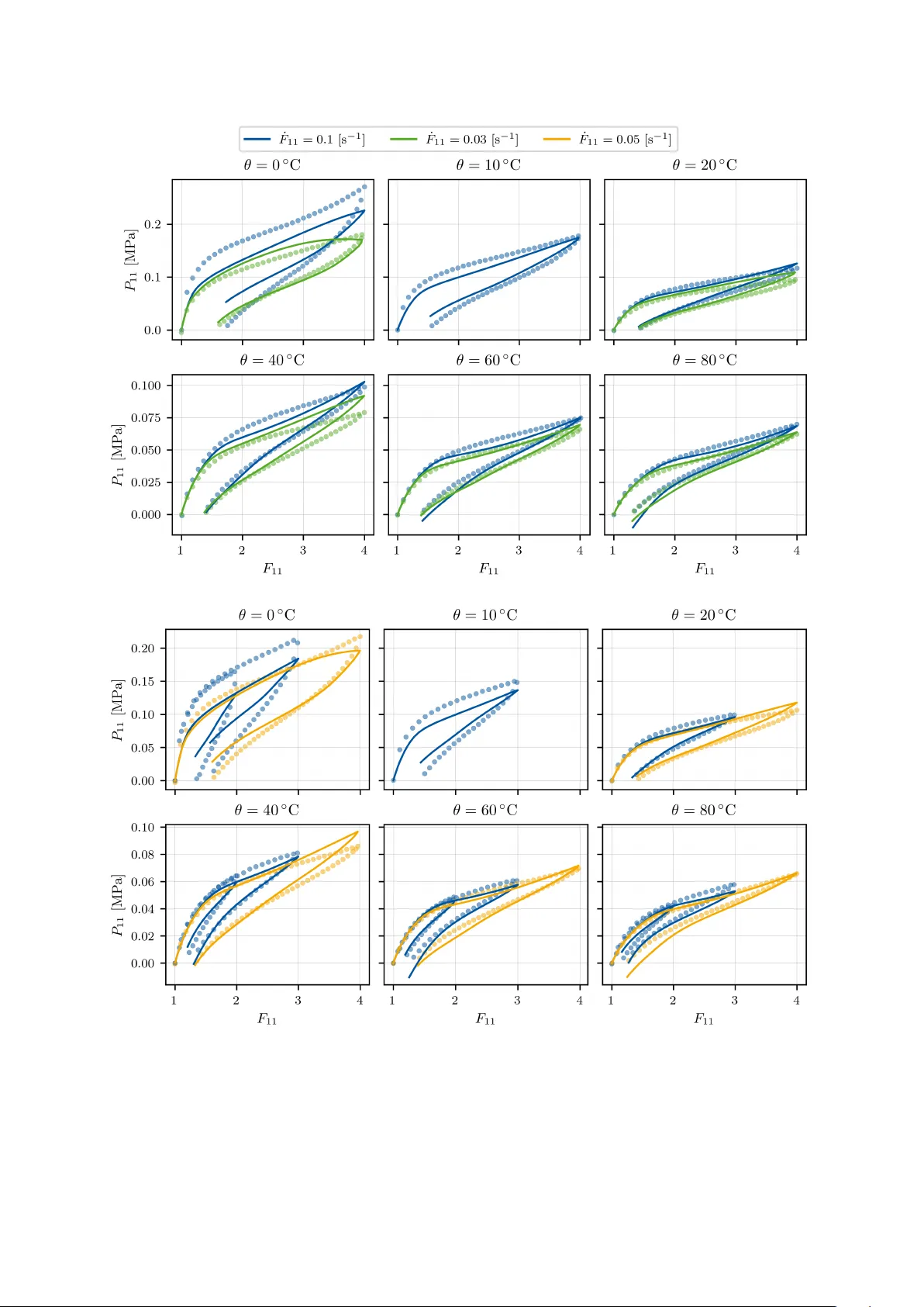
Inelastic Constituti v e K olmogoro v-Arnold Networks: A generalized frame work for automated disco v ery of interpretable inelastic material models Chenyi Ji a , Kian P . Abdolazizi b , Hagen Holthusen c , Christian J. Cyron b , d , K evin Linka a , ∗ a Computational Mechanics in Medicine, Applied Medical Engineering , RWTH Aachen Univer sity P auwelsstraße 20, 52074 Aac hen, Germany b Institute for Continuum and Material Mechanics, Hamb urg Univer sity of T echnology Eißendorfer Straße 42, 21073 Hamb urg , Germany c Institute of Applied Mechanics, University of Erlang en-Nurember g Egerlandstrasse 5, 91058 Erlang en, Germany d Institute of Material Systems Modeling, Helmholtz-Zentrum Her eon Max-Planck-Str aße 1, 21502 Geesthacht, Germany Abstract. A key problem of solid mechanics is the identiﬁcation of the constituti ve la w of a material, that is, the relation between strain and stress. Machine learning has lead to considerable advances in this ﬁeld lately . Here we introduce inelastic Constitutiv e K olmogorov–Arnold Networks (iCKANs). This nov el artiﬁcial neural network architecture can discover in an automated manner symbolic constitutive laws describing both the elastic and inelastic behavior of materials. That is, it can translate data from material testing into corresponding elastic and inelastic potential functions in closed mathematical form. W e demonstrate the advantages of iCKANs using both synthetic data and experimental data of the viscoelastic polymer materials VHB 4910 and VHB 4905. The results demonstrate that iCKANs accurately capture complex viscoelastic beha vior while preserving physical interpretability . It is a particular strength of iCKANs that they can process not only mechanical data but also arbitrary additional information available about a material (e.g., about temperature-dependent beha vior). This makes iCKANs a powerful tool to discov er in the future also how speciﬁc processing or service conditions affect the properties of materials. Keyw ords: K olmogorov-Arnold Netw orks, constituti ve modeling, inelasticity , ﬁnite strains, model disco very , symbolic re gres- sion 1 Intr oduction Accurately predicting the behavior of comple x material systems is a core challenge in engineering and the physical sciences. Con ventional computational mechanics relies on constitutive models to describe how materials respond to external stimuli. Howe ver , traditional constitutiv e models, grounded in continuum mechanics, depend on sim- plifying assumptions that often fail to capture the full complexity of real-world material beha vior—particularly for inelastic materials. Moreov er , de veloping these models is typically incremental, labor-intensiv e, and demands substantial domain expertise, with the process repeated for each no vel material system. * Corresponding author linka@ame.rwth-aachen.de 1 T o ov ercome these limitations, data-driven material modeling has emerged as a promising alternativ e, bypassing explicit constitutiv e model formulation and le veraging experimental data directly [ Fuhg et al. , 2024 ]. The model- free or direct data-driv en paradigm, pioneered by Kirchdoerfer and Ortiz [ 2016 ], eliminates predeﬁned constitutive equations in fa vor of using raw material measurements. Another avenue is symbolic regression, which constructs closed-form mathematical models from data by systematically combining analytical expressions to achiev e a bal- ance between accuracy and interpretability [ Abdusalamo v et al. , 2023 , Bomarito et al. , 2021 , Kabliman et al. , 2021 , V ersino et al. , 2017 ]. Expanding on this, EUCLID (Efﬁcient Unsupervised Constitutiv e Law Identiﬁcation and Discov ery) applies sparse re gression to a broad model library , enabling learning from full-ﬁeld data [ Flaschel , 2023 , Flaschel et al. , 2021 , 2023 ]. Recent developments hav e further enhanced these approaches to better handle noisy experimental data [ Narouie et al. , 2026 ]. A distinct class of data-driven approaches inv olves constitutiv e neural networks, which have gained prominence due to their ﬂexibility and capacity for universal function approximation [ Hornik et al. , 1989 ]. Unlike methods that impose physical constraints via the loss function [ Masi et al. , 2021 , Raissi et al. , 2019 ], these networks encode physical consistency directly through architectural design. Notable variants include Constitutive Artiﬁcial Neural Networks (CANNs) [ Linka and Kuhl , 2023 , Linka et al. , 2021 ], which fav or interpretable, sparse architectures, and Physics-Augmented Neural Networks (P ANNs) [ Linden et al. , 2023 , Rosenkranz et al. , 2024 ], which lev er- age denser , more expressiv e structures. Additional neural network classes have further broadened the modeling landscape: neural ordinary differential equations (ODEs) ha ve been used to identify polycon vex strain energy functions [ T ac et al. , 2022 ]; graph neural networks [ Maurizi et al. , 2022 ] and neural operators [ Y ou et al. , 2022 ] hav e been explored for learning complex constitutiv e and surrogate models. These methods have also found ap- plications in the design and optimization of metamaterials [ Fern ´ andez et al. , 2021 , 2022 ]. Current research pushes the boundaries by targeting increasingly complex phenomena, such as anisotropy and inelasticity [ Holthusen and Kuhl , 2026 ]. T o capture inelastic effects, the Generalized Standard Materials framew ork of fers a broad and physically grounded foundation [ Halphen and Nguyen , 1975 ]. This approach introduces an inelastic dissipation potential alongside the elastic free ener gy , governing the evolution of internal v ariables and inelastic deformation in a thermodynamically consistent manner . Integrating this framework with constituti ve neural networks has enabled the discov ery of material laws for ﬁnite-strain viscoelasticity [ As’ ad and Farhat , 2023 , Holthusen et al. , 2026 , Rosenkranz et al. , 2024 , T ac ¸ et al. , 2023 ], plasticity [ Boes et al. , 2026 , Flaschel et al. , 2025 , Jadoon et al. , 2025 ], fracture [ Dammaß et al. , 2025 ], and biological processes like growth and remodeling [ Holthusen et al. , 2025 ]. Constitutiv e models based on internal variables hav e also been successfully employed in neural ODEs and neural operators to model history- and path-dependent beha viors [ Guo et al. , 2025 , Jones et al. , 2022 ]. Furthermore, approaches such as long short-term memory networks ha ve been introduced to enhance computational ef ﬁciency in plasticity modeling [ Li et al. , 2025 ]. Constitutiv e K olmogorov–Arnold Networks (CKANs) [ Abdolazizi et al. , 2025 , Thakolkaran et al. , 2025 ] of fer a distinctive alternati ve by employing B-Splines as nonlinear , trainable activ ation functions whose mathematical forms can be extracted for interpretation [ Liu et al. , 2024 ]. The introduction of Kolmogoro v–Arnold Networks (KANs) has prompted comparativ e studies with traditional neural networks across a range of applications. KANs hav e sho wn improv ed accurac y and conv ergence in solving partial differential equations relative to multilayer perceptrons [ Abueidda et al. , 2025 , Kiyani et al. , 2025 , W ang et al. , 2025 ], with their greatest strengths evident in symbolic re gression tasks [ Ji et al. , 2024 ]. In the context of material modeling, KANs hav e been incorporated into CKANs and Input-Con ve x KANs to enhance interpretability and facilitate the discovery of con ve x strain energy functions, all while retaining the adaptability of neural network-based frameworks [ Abdolazizi et al. , 2025 , Thakolkaran et al. , 2025 ]. These developments underscore the potential of KAN-based architectures to increase the transparency of data-dri ven material models without sacriﬁcing predicti ve accuracy , though challenges in modeling 2 inelastic behavior persist. In this work, we adv ance KAN-based constitutiv e modeling by extending it to inelastic materials and introducing inelastic Constitutive K olmogorov–Arnold Networks (iCKANs). This novel approach integrates the generalized inelastic constitutive framew ork with the inherent interpretability of KANs, aiming to deli ver a rob ust, data-dri ven, and transparent model for complex inelastic behavior . iCKANs lev erage experimental stress–strain data, option- ally enriched with non-mechanical features, to uncov er the underlying elastic and inelastic potentials of materials. Crucially , the trainable activ ations of the KANs are subsequently symbolized, yielding interpretable closed-form expressions for these potentials. By enabling the automated deriv ation of symbolic inelastic potentials, pre vi- ously accessible primarily to a limited group of experts, iCKANs address a longstanding challenge in ﬁnite strain inelasticity . The ov erall workﬂow of the iCKAN frame work is illustrated in Figure 1 . Outline. Section 2 provides a concise revie w of the generalized constituti ve framework for inelastic materials at ﬁnite strains. Section 3 details the proposed iCKANs’ methodology , beginning with the foundations of K ol- mogorov–Arnold Networks and their partially input-conv ex variants, followed by their application to constituti ve modeling. Section 4 addresses the symbolic extraction process to obtain interpretable, closed-form representations of the disco vered models. Section 5 ev aluates the performance of iCKANs on both synthetic and experimental viscoelastic datasets. The paper concludes in Section 6 with a discussion of key ﬁndings and future research directions. Experimental data Kolmogor ov-Arnold Netw orks Symbolic function • T ime-dependent stress- deformation data • Non-mechanical data f f = f 1 f = f 2 f = f 3 Stretch F i Stress P i T raining with sparsiﬁcation Stress P Deformation gradient F Elastic pot. Inelastic pot. • Recurrent network architecture • Mathematical/physical constraints • (Partially) con vex splines Symboliﬁcation Stress predictions P = a ( F + b ) 2 f = f 1 f = f 2 f = f 3 Stretch F i Stress P i • Interpretability of elastic and inelastic potential • Efﬁcient numerical simulations Figure 1: Inelastic Constitutiv e Kolmogoro v-Arnold Network (iCKAN) pipeline for automated interpretable model discov ery of inelastic materials. Three-dimensional stress-strain data with optional additional features (e.g., tem- perature) collected in a feature vector f are used to train the iCKAN model, which consists of two KANs repre- senting the elastic potential ψ and the inelastic potential ω . The trained model can then be analyzed using symbolic regression to e xtract interpretable mathematical expressions. 2 Constitutiv e modeling of inelastic materials In this section, we brieﬂy re view the generalized constitutiv e frame work for inelastic materials at ﬁnite strains by Holthusen et al. [ 2023 , 2026 ], which can be seen as an equiv alence to the framework of Generalized Standard Ma- terials [ Halphen and Nguyen , 1975 ]. The frame work emplo ys the multiplicati ve decomposition of the deformation gradient and is based on tw o fundamental scalar -valued quantities, the elastic potential ψ and an inelastic potential ω [ Holthusen et al. , 2024b ]. Multiplicative decomposition. The general assumption of multiplicati ve decomposition is applied on the defor- mation gradient F , resulting into an elastic part F e and inelastic part F i , i.e., F = F e F i . Conceptually , an interme- 3 diate conﬁguration is introduced, which is reached by the inelastic deformation F i from the reference conﬁguration. The elastic deformation F e then maps the intermediate conﬁguration to the current conﬁguration. Ho we ver , the intermediate conﬁguration is ﬁctitious and not unique, since any rotation Q † ∈ S O (3) applied to the intermediate conﬁguration does not alter the physics of the resulting deformation gradient, i.e., F = F e Q † T Q † F i = F † e F † i . Fol- lowing Holthusen et al. [ 2023 , 2024b ], a unique co-rotated intermediate conﬁguration is obtained by applying the rotation of the polar decomposition of F i = R i U i to the intermediate conﬁguration, i.e., ¯ F e = F e R i = FU − 1 i , with U i and R i being the stretch part and rotation part of the inelastic deformation, respectiv ely . F F † i F † e F i F e Q † U i R i reference conﬁguration intermediate conﬁguration current conﬁguration arbitrarily rotated intermediate conﬁguration co-rotated intermediate conﬁguration B 0 B t Figure 2: Multiplicative split of the deformation gradient into elastic and inelastic part, including the non- uniqueness of the intermediate conﬁguration and the co-rotated intermediate conﬁguration [ Holthusen et al. , 2023 ]. The right Cauchy-Green deformation tensors are deﬁned as C = F T F and ¯ C e = U − 1 i CU − 1 i in the current and co-rotated intermediate conﬁguration, respecti vely . Due to the fact that ¯ C e = U − 1 i CU − 1 i serves as an unique measurement for elastic stretches, the elastic potential can be deﬁned depending on it, i.e., ψ = ψ ( ¯ C e ) , while preserving the principles of objectivity and frame indifference. T o ensure that the elastic potential is a scalar-v alued isotropic function, we deﬁne it based on the principal in variants of ¯ C e , i.e., ψ = ψ ( I ¯ C e 1 , I ¯ C e 2 , I ¯ C e 3 ) , with I ¯ C e 1 = tr( ¯ C e ) , I ¯ C e 2 = 1 2  (tr( ¯ C e )) 2 − tr( ¯ C 2 e )  , I ¯ C e 3 = det( ¯ C e ) . (1) Dissipation inequality . F ollowing the second law of thermodynamics, the dissipation D has to be non-negati ve so that thermodynamic consistency is preserv ed. This can be expressed using Clausius-Plank inequality D = S : 1 2 ˙ C − ˙ ψ ≥ 0 . By inserting the fact that the elastic potential depends on ¯ C e and applying the chain rule, we obtain D =  S − 2 U − 1 i ∂ ψ ∂ ¯ C e U − 1 i  : 1 2 ˙ C + 2 ¯ C e ∂ ψ ∂ ¯ C e : ˙ U i U − 1 i ≥ 0 , (2) which has to be fulﬁlled for any arbitrary value of ˙ C . Hence, the second Piola-Kirchhoff stress tensor and the symmetric elastic Mandel-like stress tensor are deﬁned as S = 2 U − 1 i ∂ ψ ∂ ¯ C e U − 1 i and ¯ Σ = 2 ¯ C e ∂ ψ ∂ ¯ C e , (3) respectiv ely . The ﬁrst Piola-Kirchhof f stress can be deri ved by pulling back the second Piola-Kirchhoff stress, i.e., P = FS . Moreover , by noting that ¯ Σ is symmetric, the dissipation inequality can be reduced to D = ¯ Σ : ˙ U i U − 1 i = ¯ Σ : ¯ D i ≥ 0 with ¯ D i = sym( ˙ U i U − 1 i ) . (4) 4 Evolution equation. At this stage, a suitable ev olution equation for the inelastic rate tensor ¯ D i remains to be speciﬁed. T o this end, a dual inelastic potential ω is introduced, which is assumed to be a scalar-v alued, isotropic function of the thermodynamically consistent driving force ¯ Σ , i.e., ω = ω ( ¯ Σ ) . It has been shown that if ω is constructed to be con vex, zero-valued at ¯ Σ = 0 , and non-negati ve, the reduced dissipation inequality is satisﬁed automatically [ Germain et al. , 1983 ]. While these conditions are sufﬁcient , they are not necessary to guarantee non- negati ve dissipation. Follo wing [ Holthusen et al. , 2026 ], a more general formulation is obtained by introducing an in variant-based inelastic potential of the form ω ( ¯ Σ ) = ω  I ¯ Σ 1 , q J ¯ Σ 2 , 3 q J ¯ Σ 3  , (5) which is required to be con vex, zero-v alued at its origin, and non-neg ative with respect to the three inv ari- ants * I ¯ Σ 1 = tr( ¯ Σ ) , J ¯ Σ 2 = 1 2 tr  dev( ¯ Σ ) 2  , J ¯ Σ 3 = 1 3 tr  dev( ¯ Σ ) 3  , ∂ I ¯ Σ 1 ∂ ¯ Σ = I , ∂ J ¯ Σ 2 ∂ ¯ Σ = dev( ¯ Σ ) , ∂ J ¯ Σ 3 ∂ ¯ Σ = dev  dev( ¯ Σ ) 2  . (6) Here, dev( ¯ Σ ) = ¯ Σ − 1 3 I ¯ Σ 1 I denotes the deviatoric part of a second-order tensor . It is worth emphasizing that the square and cubic roots of the second and third in variants, respecti vely , are essential to ensure non-negati ve dissipation within this frame work [ Holthusen et al. , 2026 ]. The e volution equation for the inelastic rate tensor then follows directly from the inelastic potential as ¯ D i = ∂ ω ( ¯ Σ ) ∂ ¯ Σ = ∂ ω ∂ I ¯ Σ 1 I + ∂ ω ∂ J ¯ Σ 2 dev( ¯ Σ ) + ∂ ω ∂ J ¯ Σ 3 dev  dev( ¯ Σ ) 2  . (7) Incompressible materials. For the special case of incompressible materials, i.e., det( F ) = 1 , a Lagrange multi- plier term is added to the elastic potential ψ to obtain the augmented elastic potential ˆ ψ , ˆ ψ = ψ ( ¯ C e ) − p ( I C 3 ) . (8) The term p can be considered as the hydrostatic pressure and is determined using the boundary conditions. It is important to note that the elastic part of the deformation is, in general, not incompressible, meaning that I ¯ C e 3 not necessarily remain equal to one [ Holthusen et al. , 2024b ]. 3 Inelastic Constitutiv e Kolmogor ov–Arnold Netw orks (iCKANs) Building on the constituti ve frame work presented in the pre vious section, this section e xtends the idea of CK- ANs [ Abdolazizi et al. , 2025 ] by introducing inelastic Constituti ve Kolmogoro v–Arnold Networks (iCKANs) for automatic model discovery of inelastic materials. W e start with a brief revie w of Kolmogoro v-Arnold Networks (KANs) [ Liu et al. , 2024 ] and their modiﬁed variant of monotonic input-con vex KANs [ Thak olkaran et al. , 2025 ], and then we continue with presenting partially input-con ve x KANs, in which the output is generally con vex with respect to speciﬁed inputs. Afterwards, we apply these partially input-con ve x KANs to express the elastic and inelastic potential functions of the constitutiv e material model introduced in the last section, leading to the formu- lation of iCKANs. Thus, iCKANs naturally preserve mandatory constraints and ﬂexibility due to the expression of activ ation functions via B-Splines. 3.1 Input-con vex Kolmogor ov-Ar nold Networks Serving as a promising alternati ve to mutli-layer perceptrons, KANs replace the combination of a linear layer following with a nonlinear activ ation function with a naturally nonlinear, trainable activ ation. KANs are inspired * It is worth noting that the third in variant is generally not con vex with respect to ¯ Σ . 5 by the K olmogorov-Arnold representation theorem, which states that any continuous multi variate function on a bounded domain f : [0 , 1] n → R can be represented as a ﬁnite composition of univ ariate functions f ( x 0 ) = f ( x 0 , 1 , x 0 , 2 , . . . , x 0 ,n ) = 2 n +1 X j =1 ϕ 1 , 1 ,j n X i =1 ϕ 0 ,j,i ( x 0 ,i ) ! , (9) where x 0 ,i are the elements of the input vector x 0 and ϕ 0 ,j,i : [0 , 1] → R and ϕ 1 , 1 ,j : R → R are uni variate continuous functions [ Abdolazizi et al. , 2025 , Kolmogoro v , 1961 ]. This equation can be seen as a two-layer net- work with a topology of [ n, 2 n + 1 , 1] . Extending this idea, a deeper architecture with L layers can be constructed, resulting in a KAN with the topolgy of [ n 0 , n 1 , . . . , n L ] , where n i is the number of neurons in the i -th layer . Thus, KANs can be expressed as the follo wing nested summation f ( x ) = n L − 1 X i L − 1 =1 ϕ L − 1 ,i L ,i L − 1   n L − 2 X i L − 2 =1 . . . n 2 X i 2 =1 ϕ 2 ,i 3 ,i 2 n 1 X i 1 =1 ϕ 1 ,i 2 ,i 1 n 0 X i 0 =1 ϕ 0 ,i 1 ,i 0 ( x i 0 ) !!! . . .   . (10) The activ ation function connecting the i -th neuron in the l -th layer ( l , i ) and the i -th neuron in the ( l + 1) -th layer ( l + 1 , j ) is denoted as ϕ l,j,i for l = 0 , . . . , L − 1 , i = 1 , . . . , n l and j = 1 , . . . , n l +1 . An activ ation function is deﬁned as follows ϕ l,j,i ( x ) = w b · b ( x ) + w s · s ( x ) (11) with a basis function b ( x ) , usually b ( x ) = x/ (1 + e − x ) , and a spline function s ( x ) = P i c i B i ( x ) , where c i are trainable control points and B i are B-spline basis functions. The factors w b and w s are trainable coefﬁcients. The output of neuron ( l + 1 , j ) , x l +1 ,j , is deﬁned as the sum of the inputs x l,i after transformation, i.e., x l +1 ,j = P n l i =1 ϕ l,j,i ( x l,i ) , where each input x l,i is processed by its associated univ ariate activ ation function ϕ l,j,i . For the simplicity of notation, the layer-wise mapping is deﬁned using the nonlinear function matrix Φ l as follo ws x l +1 = Φ l ( x l ) =       ϕ l, 1 , 1( • ) ϕ l, 1 , 2( • ) . . . ϕ l, 1 ,n l ( • ) ϕ l, 2 , 1( • ) ϕ l, 2 , 2( • ) . . . ϕ l, 2 ,n l ( • ) . . . . . . . . . . . . ϕ l,n l +1 , 1( • ) ϕ l,n l +1 , 2( • ) . . . ϕ l,n l +1 ,n l ( • )       x l . (12) Thus, Equation 10 can be written compactly as KAN( x ) = (Φ L − 1 ◦ Φ L − 2 ◦ · · · ◦ Φ 1 ◦ Φ 0 )( x ) . (13) 3.1.1 Fully input-con vex architectur e A function that is twice differentiable is con vex if and only if its second deriv ativ e is nonnegati ve ov er its entire domain. For instance, consider a two-layer KAN with the input x 0 = { x 0 , 1 , . . . , x 0 ,n 0 } , we can express it as the following function f ( x 0 ) = n i X j =1 ϕ 1 , 1 ,j n 0 X i =1 ϕ 0 ,j,i ( x 0 ,i ) ! . (14) The ﬁrst and second deriv atives of f with respect to x 0 ,k are giv en by ∂ f ∂ x 0 ,k = n 1 X j =1 ϕ ′ 1 , 1 ,j n 0 X i =1 ϕ 0 ,j,i ( x 0 ,k ) ! · ϕ ′ 0 ,j,k ( x 0 ,k ) , (15) ∂ 2 f ∂ x 2 0 ,k = n 1 X j =1 ϕ ′′ 1 , 1 ,j n 0 X i =1 ϕ 0 ,j,i ( x 0 ,i ) ! · ϕ ′ 0 ,j,k ( x 0 ,k ) 2 + n 1 X j =1 ϕ ′ 1 , 1 ,j n 0 X i =1 ϕ 0 ,j,i ( x 0 ,i ) ! · ϕ ′′ 0 ,j,k ( x 0 ,k ) , (16) 6 respectiv ely . Consequently , a suf ﬁcient condition for f to be conv ex with respect to the inputs x 0 is that the following criteria hold ϕ ′′ 0 ,j,i ≥ 0 ∀ i = 1 , . . . , n 0 ; ∀ j = 1 , . . . , n 1 ; ϕ ′′ 1 , 1 ,j ≥ 0 ∀ j = 1 , . . . , n 1 ; ϕ ′ 1 , 1 ,j ≥ 0 ∀ j = 1 , . . . , n 1 . (17) That is, all ﬁrst-layer activ ation functions ϕ 0 ,j,i must be conv ex, while all second-layer activ ation functions ϕ 1 , 1 ,j must be both con ve x and non-decreasing. Con vex and non-decreasing activations. Constraining all activ ations to be conv ex and monotonic non-decreasing results into a monotonic input-con vex KAN. T o satisfy the aforementioned criteria and achiev e monotonically increasing and con vex activ ations, Thakolkaran et al. [ 2025 ] proposes to constrain the control points of the B- splines activ ation functions. First, zero base functions are chosen, i.e. b ( x ) = 0 . Then, w s is constrained to be positiv e, monotonically increasing, and con vex by w ∗ s = softplus( w s ) . Finally , the control points c i are modiﬁed to become con vex coefﬁcients c ∗ i . Thus, s ∗ ( x ) = P i c ∗ i B i ( x ) is monotonically increasing and con vex, i.e., c i +2 − c i +1 ≥ c i +1 − c i ≥ 0 , ∀ i . (18) Finally , the original activ ation in Equation 11 is modiﬁed to ϕ ( x ) = w ∗ s · X i c ∗ i B i ( x ) . (19) T o ensure that the activ ations outside the initial grid range also remain con vex and monotonically increasing, linear extrapolation is applied at both ends of the grid range [ Polo-Molina et al. , 2024 , Thakolkaran et al. , 2025 ]. Generally con vex activations. The previously introduced approach provides a con vex and non-decreasing KAN- output with respect to its inputs. Howe ver , in some cases, speciﬁcally for the inelastic potential, the output is required to be con ve x with a desired stationary point. Therefore, we apply an additional activ ation function to the KAN-output to ensure the con vexity while allo wing for non-monotonic behavior . It is important to note that the network architecture remains unchanged from the monotonic input-con vex KANs and only the output of the KAN is passed through this additional activ ation function. Giv en a conv ex and non-decreasing multiv ariate function f ( x ) , one can construct a new function ˜ f ( x ) that is con ve x, zero-v alued at its origin and has a zero deriv ativ e at x = α by passing it through the following deﬁned operation H ( • ) , ˜ f ( x ) = H ( f ( x )) = f ( x ) − f ( α ) − ∇ f ( x ) | x = α · ( x − α ) , (20) For a more general case, we can apply a further manipulation step, ˆ f ( x ) = max( ˜ f ( x ) − c, 0) with c > 0 . (21) Applying the resulting functions ˜ f ( x ) and ˆ f ( x ) to the KAN-output preserve conv exity . A demonstration of this for an univ ariate simpliﬁcation is shown in Figure 3a . The proof of this theorem can be found in Appendix A.1 . 3.1.2 Partially input-con vex architectur e In general, the outputs are required to be con vex with respect to selected input arguments, but not necessarily with respect to all inputs. In particular, the elastic potential and the inelastic potential must be con vex in the in variant-based arguments, while conv exity with respect to additional non-mechanical features is not required. For this reason, we developed a partially input-conv ex KAN, as sho wn in Figure 3b [ Amos et al. , 2017 , Deschatre and W arin , 2025 ]. The output z = f ( x , y ) is con vex with respect to the input variables x = [ x 1 , x 2 , x 3 ] , but not 7 necessarily con ve x with respect to the input variable y = [ y 1 ] . This is achiev ed by modifying the ﬁrst layer of a generally input-conv ex KAN. While the activ ations corresponding to the con vex input v ariables x remain con vex and non-decreasing, the acti vations with respect to the input variable y are unconstrained. The outputs of the ﬁrst layer are then additiv ely combined and passed through the second layer . It is to note, that this implementation is a simpliﬁed v ariant of partially input-con vex networks [ Amos et al. , 2017 ], as a more generalized implementation is beyond the scope of this work. (a) Postprocessing of a con vex, non-decreasing function x 1 x 2 x 3 y 1 z (b) A partially input-con vex K olmogorov-Arnold Network Figure 3: (a) Demonstration of the postprocessing of a con vex and non-decreasing function f ( x ) to achiev e a gen- eral con vex function with the designed stationary point at x = 0 . ˜ f ( x ) is achie ved by H -operation in Equation 20 and ˆ f ( x ) is achie ved by Equation 21 . (b) A partially input-con vex Kolmogoro v-Arnold Network, where the output z is con ve x with respect to the yellow-marked input v ariables ( x 1 , x 2 , x 3 ) and unconstrained to the blue-marked input variables y 1 . 3.2 Constitutive modeling with KANs Recalling the constituti ve frame work in Section 2 , the elastic potential ψ and inelastic potential ω must be deﬁned to formulate an inelastic material. In this work, we propose using partially input-con vex KANs to model these two scalar -valued functions. Thus, we present the inelastic Constituti ve K olmogorov-Arnold Networks (iCKANs) framew ork, which can be considered an extension to the Constituti ve Kolmogoro v-Arnold Networks (CKANs) for hyperelastic materials introduced in Abdolazizi et al. [ 2025 ]. 3.2.1 Elastic potential CKANs hav e been formulated using different choices of functional bases for the elastic potential function, e.g., pricipal inv ariants and principal stretches [ Abdolazizi et al. , 2025 ]. In this work, we adopt the variant, in which the principal in variants are selected as the functional basis for constructing the KAN representing the elastic po- tential. In the original CKAN implementation, an input-monotonic KAN is employed [ Polo-Molina et al. , 2024 ]. Here, we use the previously introduced input-con vex KAN to enforce conv exity of the learned elastic potential representation. The elastic potential function ψ should be constructed polycon vex with respect to the deformation gradient F , to ensure the existence of minimizers of the elastic potential function. T o achieve a polycon vex elastic potential function, the input arguments of the KAN must be polycon vex in F [ Hartmann and Nef f , 2003 ]. It is e vident that the elastic potential should be dependent on the principal in variants of the elastic right Cauchy-Green deformation 8 tensor in the co-rotated intermediate conﬁguration ¯ C e = U − 1 i CU − 1 i . For nearly incompressible materials, it is common practice to decouple the volumetric and isochoric parts of the elastic deformation [ Flory , 1961 , Holthusen et al. , 2024b ]. Therefore, the polycon vex modiﬁed elastic inv ariants ( ˆ I ¯ C e 1 , ˆ I ¯ C e 2 , ˆ I ¯ C e 3 ) are then deﬁned using the principal in variants ( Equation 1 ) as [ Hartmann and Nef f , 2003 , Holthusen et al. , 2024a ] ˆ I ¯ C e 1 = ˜ I ¯ C e 1 − 3 , ˆ I ¯ C e 2 = ( ˜ I ¯ C e 2 ) 3 / 2 − 3 3 / 2 , ˆ I ¯ C e 3 = ( J ¯ C e − 1) 2 , (22) with J ¯ C e = q det( ¯ C e ) , ˜ I ¯ C e 1 =  J ¯ C e  − 2 / 3 I ¯ C e 1 , ˜ I ¯ C e 2 =  J ¯ C e  − 4 / 3 I ¯ C e 2 . (23) Thus, a polycon vex elastic potential is constructed using the modiﬁed inv ariants of ¯ C e as input argument for the input-con ve x KAN ψ = ψ ( ¯ C e ) = ψ ( ˆ I ¯ C e 1 , ˆ I ¯ C e 2 , ˆ I ¯ C e 3 ) . (24) It is to note that the polycon ve xity with respect to the arguments is not a necessary condition for the elastic potential to fulﬁll the physics, but rather a con venient assumption for the potential minimization. Furthermore, a proof that the output elastic potential ψ and its deri vati ve are zero at undeformed state can be found in Appendix A.2 3.2.2 Inelastic potential What remains to be deﬁned is the inelastic potential ω , which go verns the e volution equation of the inelastic strain. T o satisfy thermodynamic consistency , the inelastic potential ω must be zero-valued at its origin, nonnegati ve and con ve x with respect to its arguments, which are the modiﬁed stress in variants of the elastic Mandel stress ¯ Σ ( Equation 6 ), ˆ I ¯ Σ 1 = I ¯ Σ 1 , ˆ J ¯ Σ 2 = q J ¯ Σ 2 , ˆ J ¯ Σ 3 = 3 q J ¯ Σ 3 . (25) Thus, we deﬁne the inelastic potential dependent on the modiﬁed stress in variants as ω = ω ( ¯ Σ ) = ω  ˆ I ¯ Σ 1 , ˆ J ¯ Σ 2 , ˆ J ¯ Σ 3  . (26) Unlike the pre viously mentioned condition for the elastic potential, the inelastic potential must be con vex with respect to the modiﬁed stress in variants for the dissipation inequality to be fulﬁlled. Noteworth y , we could enhance the existing arguments as long as the con vexity condition is satisﬁed. For instance, to increase network ﬂexibility and expressibility , the negati ve stress in variants, or additional in variants, e.g., the principal in variants [ Holthusen et al. , 2026 ], can be appended to the argument of the inelastic potential network. These alternati ve constructions are presented in Appendix A.3 . Follo wing the approach of the previously presented general input-conv ex KAN, a con vex, zero-valued and non- negati ve inelastic potential ω is constructed by applying H -operator ( Equation 20 ) as a postprocessing acti vation on the output of the monotonic input-con ve x KAN, ω KAN , i.e., ω = H ( ω KAN ) = ω KAN − ω KAN   ¯ Σ = 0 −    ∂ ω /∂ ˆ I ¯ Σ 1 ∂ ω /∂ ˆ J ¯ Σ 2 ∂ ω /∂ ˆ J ¯ Σ 3           ¯ Σ =0 ·    ˆ I ¯ Σ 1 ˆ J ¯ Σ 2 ˆ J ¯ Σ 3    . (27) As pre viously stated, a further postprocessing step shown in Equation 21 can be applied to ω . Due to the special construction of the inelastic potential, which allo ws for a zero interval of the deriv ativ e of inelastic potential, meaning that no inelastic response is acti vated until a certain stress le vel is reached, and one single iCKAN model is suf ﬁcient to represent a viscoelastic material under relaxation. This can be represented as the rheological model in Figure 4 . The elastic potential ψ is associated with the spring, and the inelastic potential ω with the dashpot. Howe ver , at this end, the training of this parameter c is unstable, leading us to choose to leave out this particular step and combine two iCKANs in parallel to express a viscoelastic material. 9 ψ ( ¯ C e ) ω ( ¯ Σ ) Figure 4: Representation of the iCKAN formulation in the form of a Maxwell model. The elastic potential ψ is associated with the spring, and the inelastic potential ω with the dashpot. 3.2.3 Featur e dependency The appropriate functional form of the elastic and inelastic potential generally depend on material descriptors such as composition, microstructure, or processing conditions. W e collect this information in a feature vector f and augment the arguments of both the elastic and inelastic potentials as ψ = ψ ( ˆ I ¯ C e 1 , ˆ I ¯ C e 2 , ˆ I ¯ C e 3 , f ) and ω = ω  ˆ I ¯ Σ 1 , ˆ J ¯ Σ 2 , ˆ J ¯ Σ 3 , f  . (28) This feature is solely non-mechanical and neither the elastic potential nor the inelastic potential is con ve x with respect to it. 3.2.4 Numerical implementation The ev olution equation deﬁned by the inelastic rate tensor, D i = ∂ ω /∂ Σ (see also ( 7 )), is solved numerically . The exponential integrator map has been sho wn to be particularly effecti ve for inelastic problems and in the ﬁnite strain regime [ Holthusen et al. , 2025 , 2026 ]. Numerically , this ev olution equation can be integrated using either explicit or implicit time integration schemes. In the explicit formulation, the current inelastic stretch tensor U i,t depends solely on the pre vious time step and the current increment. Con versely , the implicit formulation introduces a nonlinear dependence on both current and pre vious states, necessitating the solution of a nonlinear system at each time step. Although the implicit scheme is generally less sensitive to time step size, it is computationally more demanding than the explicit approach. T o accelerate the solution of the nonlinear system in the implicit scheme, a Liquid Time Constant Network can be employed as an alternativ e to the traditional iterati ve Newton solver [ Holthusen and K uhl , 2026 ]. Section 5 presents a side-by-side comparison of both formulations using synthetic data. Giv en its superior robustness and performance across all numerical examples discussed in the following section, this work primarily focuses on explicit time integration. Detailed information on the implicit time integration scheme is pro vided in Appendix A.6 . Explicit time integration. F ollowing the explicit integration scheme, the inelastic right Cauchy-Green tensor at the current timestep, C i,t , is approximated using the inelastic strain rate from the previous timestep, D i,t − 1 , as C i,t = U i,t − 1 exp(2 ∆ t D i,t − 1 ) U i,t − 1 , U i,t = C 1 / 2 i,t , (29) where ∆ t is the time increment between timestep t − 1 and t [ Holthusen et al. , 2026 ]. The ov erall architecture of the explicit iCKAN is illustrated in Figure 5 . Notew orthy , while a T yler expansion might be sufﬁcient to generate the matrix squre-root under moderate deformations, a closed-form representation should be utilized for nonlinear ﬁnite strains [ Holthusen et al. , 2026 , Hudobivnik and K orelc , 2016 ]. The explicit scheme proves to be computationally efﬁcient, as no iterativ e solver is required. Stability is controlled through the selection of the time increment ∆ t , offering a straightforw ard and transparent mechanism for maintaining numerical robustness. Initial grid range. Since the KAN activ ation functions are represented by B-splines deﬁned on ﬁx ed domains, suitable input grid range must be speciﬁed for each input dimension. In the present recurrent formulation, these effecti ve inputs are not kno wn a priori, as they are generated during the forward pass and ev olve throughout training. W e therefore adopt a data-driven initialization strategy to estimate appropriate grid ranges from physically 10 ¯ C e,t − 1 ¯ Σ ¯ D i ¯ U i ¯ C e C t − 1 , U i,t − 1 State F t , ∆ t Input C t , U i,t State P t Output ψ t − 1 ψ t ω t − 1 Figure 5: Explicit iCKAN architecture at timestep t . The inputs at each step are the current deformation gradient and time increment ( F t , ∆ t ) together with the state variables ( C t − 1 , U i,t − 1 ) from the previous step. The KAN models for the elastic potential ψ and the inelastic potential ω are ev aluated to update the state variables according to Equation 29 . The updated state is then propagated to the next time step. In addition, the output stress P is computed by ev aluating the elastic potential ψ with the updated state variables. meaningful tensor inv ariants computed on the training data. The detailed construction and its justiﬁcation are provided in Appendix A.4 . Further details of computation reﬁnements, i.e. the modiﬁed deﬁnitions of square root and cubic root and the numerical implementation of the matrix square roots, are summarized in the Appendix A.5 . 4 Symbolic constitutiv e modeling T o obtain an interpretable closed-form e xpression of the constituti ve models, the trained KANs for the elastic and inelastic potentials can be symboliﬁed after model training. In this section, we brieﬂy re vie w the sparsiﬁcation and symboliﬁcation process, for more details, please refer to [ Abdolazizi et al. , 2025 , Liu et al. , 2024 ]. Sparsiﬁcation and pruning. T o achiev e a sparse network structure, L1 regularization is applied to the trainable parameters, which in this case correspond to the control points of the B-Spline acti vations. Furthermore, pruning methods can be applied to the trained KANs to remove less important connections or nodes, further simplifying the model. This can help improv e interpretability by focusing on the most relev ant features and reducing the ov erall complexity of the network. Symboliﬁcation of con vex, monotonic activations. The trained KANs can be symboliﬁed into closed-form math- ematical expressions using symbolic re gression techniques. The symboliﬁcation process aims to ﬁnd a mathemat- ical expression that closely approximates the behavior of the trained KANs while being more interpretable. This is achiev ed by searching through a space of mathematical expressions f l,j,i and selecting the one that best ﬁts the data generated by the KANs. For each activ ation ϕ l,j,i , we aim to ﬁnd the optimal symbolically approximated activ ation, y l,j,i = c l,j,i · ( f l,j,i ( a l,j,i · x l,i + b l,j,i )) + d l,j,i , (30) so that the squared error between ϕ l,j,i and y l,j,i is minimized. For this, a library of designed symbolic functions is provided and additional afﬁne parameters ( a, b, c, d ) l,j,i are introduced. Furthermore, the parameters ( a, c ) l,j,i 11 are constrained to be nonnegati ve to preserv e the monotonicity and con vexity of the acti vation functions. Due to the recurrent network architecture, only the activ ation values from the ﬁnal forward pass (i.e., the last time step) are retained. Consequently , a forward pass over the entire dataset is required to recover activ ation values across the full input domain. Otherwise, the e xtracted symbolic function does not f aithfully reproduce the original B-spline activ ation. 5 Numerical examples In this section, we validate the proposed iCKAN frame work on synthetic and experimental datasets, including VHB 4910 [ Hossain et al. , 2012 ] and temperature-dependent VHB 4905 polymer [ Liao et al. , 2020 ]. These examples demonstrate that iCKAN capture inelastic material behaviors and additional feature effects. Symbolic expressions of the trained iCKANs are presented to highlight the interpretability of the approach. For all training processes, the initial weights and biases of the KANs are initialized using a uniform random distribution. The loss function is deﬁned as the normalized mean squared error (NMSE) between the predicted and target ﬁrst Piola-Kirchhoff stresses, P and ˆ P , respecti vely . The error is normalized by the largest absolute entry of the target stress for each batch sample, computed o ver all time steps and stress components. Formally , the loss is giv en by L stress = 1 B T S B X b =1 T X t =1 S X s =1       P b,t,s − ˆ P b,t,s max t,s   ˆ P b,t,s         2 , (31) where B is the batch size, T is the number of time steps, and S is the number of stress components. The AMS- GRAD optimizer [ Reddi et al. , 2019 ], which combines the beneﬁts of ADAM and RMSPR OP , is utilized for train- ing in combination with a cyclic learning rate scheduler [ Smith , 2017 ], where the learning rate cyclically varies between a base learning rate and a maximum learning rate ov er a gi ven step size. Furthermore, L1 regularization is applied to achiev e a sparse network and gradient clipping is applied to pre vent gradient explosion. 5.1 V eriﬁcation on synthetic data Synthetic data are generated using an explicit time integration scheme on an iCKAN, where the corresponding KANs are replaced by analytical formulas. A Neo-Hookean free energy ψ = 0 . 5 · ˆ I ¯ C e 1 + 0 . 5 · ˆ I ¯ C e 3 is assumed for the elastic potential, and the inelastic potential is deﬁned as ω = 0 . 1 · ( ˆ I ¯ Σ 1 ) 2 + ( ˆ J ¯ Σ 2 ) 2 . W e only change the ﬁrst entry of the deformation gradient from the undeformed state and apply a cyclic loading case of tension, relaxation, compression and relaxation. W e set the maximum stretches to F max 11 = { 1 . 1 , 1 . 2 , 1 . 3 } and set the time of tensile loading to t load = { 0 . 2 , 0 . 5 , 1 . 0 } s, resulting into different strain rates. At the end, the dataset consists of deformation gradients F and time increments ∆ t as inputs and the corresponding ﬁrst Piola–Kirchhoff stresses P as outputs. Model training. For the training, we use only the tensile loading and relaxation part of the datasets with t load = { 0 . 2 , 0 . 5 } s for all three stretch levels. W e consider an iCKAN which can be illustrated as the rheological model in Figure 4 . Both the elastic and inelastic potentials are modeled by input-conv ex KANs with topology [3,1]. The initial grid ranges are approximated as described in Appendix A.4 . T o improve robustness and account for previously unseen input ranges, the grid bounds are extended by 20%. For arguments that may attain negati ve values, the lower bound is chosen symmetrically with respect to the upper bound. W e examine both the explicit and implicit v ariant of iCKAN. Training is performed with an initial learning rate of 5 · 10 − 4 and a cyclic scheduler between 5 · 10 − 5 and 1 · 10 − 4 with a step size of 50 iterations. L1 regularization of 10 − 5 and gradient clipping at 0.1 are applied. For the implicit iCKAN, the evolution penalty with λ ev o = 1000 and increased by a factor of two ev ery 250 epochs. 12 Symboliﬁcation. W e demonstrate the symboliﬁcation on the trained iCKAN. All activ ations in the KAN for elastic potential are approximated using a library of conv ex, non-decreasing functions f ( x ) on [0 , ∞ ) . This process is illustrated in Figure 6a and the full set of candidate functions is listed in Appendix A.7 . The symbolic formulation of the output inelastic potential ω KAN can be obtained analogously while the enforcement of con vexity , zero-v alued at its origin and non-negati vity is achie ved by applying H -operator in Equation 27 on the symboliﬁed ω KAN . Howe ver , for the presented single-layer KAN, the network output reduces to ω KAN = n 0 X i =1 ϕ 0 ,j,i ( x 0 ,i ) , (32) In this case, it is equi valent to apply H -operator to the full output ω KAN or to each activ ation function ϕ 0 , 0 ,i , H ( ω KAN ) = n 0 X i =1 H ( ϕ 0 , 0 ,i ( x 0 ,i )) . (33) Consequently , the desired inelastic potential can be obtained by directly symbolizing H ( ϕ 0 ,j 0 ,i ) using candidate functions that are conv ex, nonnegati ve, and zero at the origin (see Appendix A.7 ). The resulting symbolic e xpres- sion inherently satisﬁes all constraints without requiring further postprocessing, i.e., ω = ω KAN . This procedure is illustrated in Figure 6b . Howe ver , this simpliﬁcation does not apply to deeper network architectures. The ﬁnal symbolic expressions for the elastic and inelastic potential functions identiﬁed by the implicit and ex- plicit iCKAN approaches are presented in Figure 7 c. The corresponding predictions are shown in Figure 7 a and Figure 7 b. More detailed results re garding model validation with synthetic data are provided in Appendix A.8 . The predictions generated by iCKAN align closely with both the training and test datasets. Interestingly , both time integration approaches produced comparable results on this simple synthetic dataset, with only minor differences in the discov ered symbolic forms of the elastic and inelastic potentials. This demonstrates that, in principle, either approach leads to similar outcomes and can be effecti vely employed in practice to discover material models using iCKANs. ˆ I ¯ C e 1 ˆ I ¯ C e 2 ˆ I ¯ C e 3 ψ KAN symb . − → ˆ I ¯ C e 1 ˆ I ¯ C e 2 ˆ I ¯ C e 3 ψ KAN (a) Symboliﬁcation for elastic potential ˆ I ¯ Σ 1 ˆ J ¯ Σ 2 ˆ J ¯ Σ 3 ω KAN symb . − → ˆ I ¯ Σ 1 ˆ J ¯ Σ 2 ˆ J ¯ Σ 3 ω KAN (b) Symboliﬁcation for inelastic potential Figure 6: Symboliﬁcation of the activ ation functions of the trained iCKAN on synthetic data. Black curves de- note the learned B-spline acti vations, and red curves their symboliﬁed approximations. (a) KAN-based elastic potential: conv ex, non-decreasing acti vations are approximated by symbolic functions that preserve con vexity and monotonicity over the admissible domain. (b) KAN-based inelastic potential: acti vations are transformed by H -operator ( Equation 20 ) and then symboliﬁed by con ve x, nonne gativ e functions that are zero-valued at the origin. 13 (a) Explicit time integration (b) Implicit time integration t [s] Elastic potential ψ ( ¯ C e ) = a · ˆ I ¯ C e 1 + b · ˆ I ¯ C e 2 + c · ˆ I ¯ C e 3 Material parameters Explicit Implicit a b c a b c 0.0 0.2194 0.5027 0.2722 0.1093 0.5255 Inelastic potential ω ( ¯ Σ ) = a · ( ˆ I ¯ Σ 1 ) 2 + b · ( ˆ J ¯ Σ 2 ) 2 + c · ( ˆ J ¯ Σ 3 ) 2 Material parameters Explicit Implicit a b c a b c 0.109 0.9394 0.4286 0.1045 1.2613 0.6397 (c) Discover ed elastic and inelastic potential functions for the synthetic dataset Figure 7: Results of the symboliﬁed iCKAN on synthetic compressible material data using (a) the explicit time integration scheme and (b) the implicit time integration scheme, using the e xpressions presented in T able (c). The gray regions in (a) and (b) indicate the range of the training data, and the colored dots represent the corresponding reference data. 5.2 Model discovery f or experimental data T o access the practical applicability of iCKANs, we e xamine the frame work on experimental data of viscoelastic polymers. Due to the fact that the provided experimental data are one-dimensional, the information of volumetric modes are lacking. Thus, we assume incompressible materials [ Abdolazizi et al. , 2024 , Holthusen et al. , 2026 ]. The detailed hyperparameters are provided in Appendix A.9 , together with the loss con vergence curves ov er the training epochs. 5.2.1 Viscoelastic model disco very of VHB 4910 polymer V ery-High-Bond (VHB) 4910 is a polymer exhibiting highly nonlinear and viscoelastic behavior . Experimental uniaxial loading–unloading data for VHB 4910 are reported by Hossain et al. [ 2012 ] for four maximum stretch lev els, F 11 = { 1 . 5 , , 2 . 0 , , 2 . 5 , , 3 . 0 } , tested under three different stretch rates, ˙ F 11 = { 0 . 01 , , 0 . 03 , , 0 . 05 } s − 1 . In our framework, rate dependence is incorporated directly through the network input pair ( F , ∆ t ) , allowing the model to learn time-dependent behavior without introducing e xplicit viscosity terms. 14 T o capture more comple x material beha viors, we utilize two iCKANs in parallel, moti vated by classical rheological representations of viscoelastic materials, as illustrated in Figure 8 b . In continuum mechanics, the total stress response of viscoelastic solids is often represented as the superposition of multiple parallel mechanisms, each corresponding to a distinct elastic potential and inelastic potential. The two branches of the parallel structure are index ed by superscripts 1 ( • ) and 2 ( • ) , which share the same input deformation gradient F . Each branch learns its o wn elastic potential i ψ ( i ¯ C e ) and inelastic potential i ω ( i ¯ Σ ) , while enforcing thermodynamic consistenc y . The stress contribution i P of each branch is obtained consistently via differentiation of the learned potentials. The total stress response is then computed as the additi ve superposition P = 1 P + 2 P , which is consistent with classical rheological network models and enables the representation of multiple concurrent elastic and inelastic mechanisms with different characteristic responses. Model training . For training, we use the dataset corresponding to the highest stretch lev el, F 11 = 3 . 0 , while the remaining stretch le vels are reserved for v alidation to assess generalization for unseen data. W e approximate the initial grid range as previously and e xtend them by 20% on both sides. ˆ I 1 ¯ C e 1 ˆ I 1 ¯ C e 2 ˆ I 1 ¯ C e 3 1 ψ KAN (a) 1 ψ ( 1 ¯ C e ) ˆ I 1 ¯ Σ 1 ˆ J 1 ¯ Σ 2 ˆ J 1 ¯ Σ 3 1 ω KAN (b) 1 ω ( 1 ¯ Σ ) ˆ I 2 ¯ C e 1 ˆ I 2 ¯ C e 2 ˆ I 2 ¯ C e 3 2 ψ KAN (c) 2 ψ ( 2 ¯ C e ) 1 ψ ( 1 ¯ C e ) 2 ψ ( 2 ¯ C e ) 1 ω ( 1 ¯ Σ ) 2 ω ( 2 ¯ Σ ) P = 1 P + 2 P (a) Discover ed model for VHB4910 polymer (b) Rheological model Figure 8: KAN architectures of discovered model for VHB4910 polymer . (b) Rheological model consisting two iCKANs in parallel combination. Both iCKAN branches recei ve the same input deformation gradient F and each learns an elastic potential and an inelastic potential. The ﬁrst branch identiﬁes 1 ψ ( 1 ¯ C e ) and 1 ω ( 1 ¯ Σ ) and produces the stress 1 P while preserving thermodynamic consistency . The second branch identiﬁes 2 ψ ( 2 ¯ C e ) and 2 ω ( 2 ¯ Σ ) and produces the stress 2 P under the same thermodynamic constraints. The total stress response is obtained by summing the stresses of both branches, P = 1 P + 2 P . Symboliﬁcation and results. At the end, we utilize the same library of con vex, monotoonic functions as in the previous section to symbolify the activ ations of the trained model. The symboliﬁed discovered KAN models of the corresponding elastic and inelastic potentials are shown in Figure 8 a with their corresponding symbolic functions in Figure 9 b . The predicted results of the symboliﬁed iCKAN model are shown in Figure 9 a. 15 T raining T esting T esting T esting (a) Predictions of the symboliﬁed iCKANs f or VHB 4910 Elastic potential 1 ψ ( 1 ¯ C e ) = a · exp( b · ˆ I 1 ¯ C e 1 ) + c · ˆ I 1 ¯ C e 2 Material parameters a b c 34.654 0.1204 3.7902 Inelastic potential 1 ω ( 1 ¯ Σ ) = H ( a · exp( b · exp( c · ˆ J 1 ¯ Σ 2 ))) Material parameters a b c 0.0195 0.0002 0.036 Elastic potential 2 ψ ( 2 ¯ C e ) = a · ˆ I 2 ¯ C e 1 + b · ˆ I 2 ¯ C e 2 + c · exp( d · ˆ I 2 ¯ C e 1 ) Material parameters a b c d 2.5911 1.8997 68.73 0.0299 (b) Discover ed elastic and inelastic potential functions for VHB 4910 polymer Figure 9: Discov ered model for VHB4910 polymer . (a) Predictions by the symboliﬁed trained iCKAN under three different constant loading/unloading rates, denoted as ˙ F 11 . The prediction of the trained iCKAN model is represented by the solid lines and the experimentally measured data is represented by dots in corresponding colors. Only the experimental data corresponding to F max 11 = 3 . 0 [-] are utilized for training. (b) listes the corresponding symbolic functions. 5.2.2 Thermo-viscoelastic model discovery of VHB 4905 polymer Building on the previous section, we next consider the identiﬁcation of material models augmented by an additional feature vector f . Our goal is to ﬁnd a single iCKAN expression capable of describing the material behavior under varying non-mechanical conditions. T o this end, we study the VHB 4905 polymer, which exhibits highly 16 deformable, viscoelastic, and temperature-sensitive behavior . Uniaxial e xperimental data for VHB 4905 polymer at different temperatures, θ = { 0 , 10 , 20 , 40 , 60 , 80 } ◦ C, under multiple strain rates, F 11 = { 0 . 03 , 0 . 05 , 0 . 1 } s − 1 , and maximum stretch ratios, F 11 = { 2 . 0 , 3 . 5 , 4 . 0 } , are reported in [ Liao et al. , 2020 ]. T emperature as feature. The strain rate and deformation information are naturally incorporated into the model inputs. In addition, the temperature θ is explicitly included as a feature in the arguments of the elastic potential, i.e., [ Abdolazizi et al. , 2025 ] i ψ ( i ¯ C e ) = i ψ ( ˆ I i ¯ C e 1 , ˆ I i ¯ C e 2 , ˆ I i ¯ C e 3 , θ ) . (34) It is important to note that this approach differs from classical thermo-mechanical constitutive modeling, where temperature is included via either thermal strain decomposition or temperature-dependent material parameters. Instead, this feature-augmented construction provides a general, data-driven mechanism to capture the inﬂuence of unkno wn non-mechanical factors on the elastic potential, and consequently , on the material stress response. The initial grid range for this temperature feature is set directly by the experimental temperature range, [0 , 80] ◦ C, while the grid ranges for the in variants are approximated as before and extend by 20% on both ends. Although it is reasonable to assume the feature has inﬂuence on both elastic and inelastic potential, we choose to omit it for the inelastic potential due to network rob ustness. Symboliﬁcation. W e symbolify the trained activ ations, except for those corresponding to the temperature feature in the ﬁrst layer of each KAN for elastic energy , using the same library of con vex, monotonic functions as in the previous section. The resulting KAN architectures are shown in Figure 10 . For each branch, there remains an activ ation function associated with temperature in the elastic potential i ψ ( i ¯ C e ) , which we denote as 1 g ( θ ) and 2 g ( θ ) for the ﬁrst and second branch, respecti vely . ˆ I 1 ¯ C e 1 ˆ I 1 ¯ C e 2 ˆ I 1 ¯ C e 3 θ 1 ψ KAN (a) Model of 1 ψ ( 1 ¯ C e ) ˆ I 1 ¯ Σ 1 ˆ J 1 ¯ Σ 2 ˆ J 1 ¯ Σ 3 1 ω KAN (b) Model of 1 ω ( 1 ¯ Σ ) ˆ I 2 ¯ C e 1 ˆ I 2 ¯ C e 2 ˆ I 2 ¯ C e 3 θ 2 ψ KAN (c) Model of 2 ψ ( 2 ¯ C e ) ˆ I 2 ¯ Σ 1 ˆ J 2 ¯ Σ 2 ˆ J 2 ¯ Σ 3 2 ω KAN (d) Model of 2 ω ( 2 ¯ Σ ) Figure 10: Discovered model for VHB4905 thermo polymer As these activ ations are not constrained to be monotonic or con ve x, their shapes can be arbitrary . T o capture this ﬂexibility , we adopt higher-order polynomial functions. This approach allo ws us to automatically discover a symbolic expression for 1 g ( θ ) . For 2 g ( θ ) , howe ver , a single symbolifc function did not provide sastisfactory ﬁt. Therfore, we allow for piecewise symboliﬁcation, and manually approximate it using two piece wise quadratic functions deﬁned ov er the temperature interv als [0 , 40) and [40 , 80] ◦ C, respecti vely . The coef ﬁcients are chosen such that C 1 -continuity is enforced at θ = 40 ◦ C. Results. The predicted results of the sym boliﬁed iCKAN model are sho wn in Figure 11 . The symboliﬁed formula for the discov erd model are listed in Figure 12 . 17 (a) T raining data (b) T esting data Figure 11: (a) T raining set and (b) v alidation set of discovered model for the experimental data of VHB 4905 polymer under three different constant loading/unloading rates, denoted as ˙ F 11 . The prediction of the trained iCKAN model is represented by the solid lines and the experimentally measured data is represented by the dotts in the corresponding colors. 18 The iCKAN frame work successfully captures the temperature-dependent viscoelastic behavior of VHB 4905. Symboliﬁcation of the learned acti vations provides interpretable functional forms, rev ealing how temperature in- ﬂuences the elastic potentials in each branch. Overall, this demonstrates the model’ s ability to combine predicti ve accuracy with physical interpretability under v arying en vironmental conditions. Elastic potential 1 ψ ( 1 ¯ C e ) = a · exp( b · ˆ I 1 ¯ C e 1 + c · ˆ I 1 ¯ C e 2 + g ( θ )) Material parameters a b c 0.0349 0.0855 0.0864 T emperature dependency 1 g ( θ ) = 10 . 0746 · (0 . 5239 − 0 . 0111 · θ ) 3 Inelastic potential 1 ω ( 1 ¯ Σ ) = H ( a · exp( b · exp( c · ˆ J 1 ¯ Σ 2 ) + d · exp( e · ˆ J 1 ¯ Σ 3 ))) Material parameters a b c d e 31.918 0.1077 4.7 0.0382 10.0 Elastic potential 2 ψ ( 2 ¯ C e ) = a · exp( b · ˆ I 2 ¯ C e 2 + c · exp( d · ˆ I 2 ¯ C e 3 ) + 2 g ( θ )) Material parameters a b c d 0.319 0.0261 0.0921 10.0 T emperature dependency 2 g ( θ ) =      − 1 . 7498 · 10 − 4 · θ 2 + 3 . 256 · 10 − 3 · θ − 1 . 8712 · 10 − 1 , 0 ≤ θ < 40 − 3 . 51 · 10 − 5 · θ 2 + 2 . 344 · 10 − 3 · θ − 7 . 9019 · 10 − 2 , 40 ≤ θ ≤ 80 Inelastic potential 2 ω ( 2 ¯ Σ ) = H ( a · exp( b · ˆ I 2 ¯ Σ 1 + c · exp( d · ˆ J 2 ¯ Σ 2 ))) Material parameters a b c d 0.0589 0.2543 0.0264 2.8013 Figure 12: Discovered elastic and inelastic potential functions for VHB 4905 thermo polymer . 6 Discussion Dev eloping accurate and interpretable constitutiv e models for materials undergoing nonlinear inelastic deforma- tion, particularly at ﬁnite strains, remains a central challenge in computational mechanics. Although recent ad- vances in data-driven modeling ha ve accelerated model disco very , a persistent trade-off exists between predicti ve accuracy and physical interpretability . Thermodynamically consistent approaches often rely on highly ﬂexible neural networks, which can lack transparency , or on symbolic methods with limited expressiv eness [ Flaschel et al. , 2023 , Holthusen et al. , 2026 ]. This work bridges this divide by introducing inelastic Constitutiv e K ol- mogorov–Arnold Networks (iCKANs), which combine a generalized inelastic constitutive frame work with the interpretability of Kolmogoro v–Arnold Networks (KANs). This inte gration enables iCKANs to achie ve predicti ve accuracy , interpretability , and robust extrapolation simultaneously . Their ﬂexible architecture also facilitates sym- bolic extraction of learned potentials. Building upon pre vious KAN-based framew orks for hyperelastic materials, iCKANs establish a new paradigm for interpretable, data-dri ven discov ery of inelastic material models [ Abdolazizi et al. , 2025 , Thakolkaran et al. , 2025 ]. Interpr etability . The iCKAN framework shares the constituti ve structure of inelastic Constitutiv e Neural Net- works (iCANNs) [ Holthusen et al. , 2026 ], b ut dif fers fundamentally in its representation of the elastic and inelastic potentials. Whereas iCANNs employ custom-built con ve x neural networks, iCKANs use input-con vex KANs, en- abling a more compact and expressi ve formulation. The use of trainable B-spline activ ations enables iCKANs to achiev e high expressi veness with substantially reduced network complexity . A major advantage of KANs is their built-in support for activation-le vel symbolic regression, which facilitates the direct extraction of interpretable, closed-form analytical expressions for both elastic and inelastic potentials. This capability preserv es ﬂexibility in 19 data-driv en discov ery while yielding transparent, ph ysically meaningful models with strong predictive performance [ Abdolazizi et al. , 2025 ]. Furthermore, iCKANs naturally accommodate additional non-mechanical features, such as temperature, whose effects can be extracted as explicit mathematical expressions, providing v aluable physical insight. Extrapolability . The combination of a thermodynamically consistent constitutiv e frame work and con ve x-network architecture ensures that the learned elastic and inelastic potentials satisfy essential physical constraints across their entire input domain. Importantly , these constraints are retained in the closed-form symbolic expressions obtained through the KAN symboliﬁcation process. This structure enhances robustness and enables physically consistent extrapolation beyond the training regime [ Abdolazizi et al. , 2025 ]. As demonstrated in synthetic benchmarks (Section 5.1 ), models trained on limited deformation data can still provide reliable predictions for unseen, larger deformations using both the spline-based KAN and its symbolic form. Computational efﬁciency . By promoting sparsity in the KAN architecture, the symbolic regression process yields concise, closed-form expressions for both elastic and inelastic potentials. These analytical formulations can be seamlessly integrated into ﬁnite element solvers, eliminating the need for network ev aluation during simulation. As a result, the iCKAN approach introduces no additional computational overhead at deployment [ Abdolazizi et al. , 2025 ]. Choice of input representation. This study employs the principal in variants of the elastic right Cauchy–Green tensor as inputs for the elastic potential, but alternative objectiv e representations—such as principal stretches—are equally v alid in the iCKAN formulation [ Abdolazizi et al. , 2025 ]. For the inelastic potential, inv ariant-based stress measures are used, with the option to augment input sets by combining stress and deformation in variants. The selection of input representation inﬂuences both predicti ve accuracy and interpretability , and a systematic compar- ison across different material classes is a promising direction for future research [ Holthusen et al. , 2026 ]. Predicti ve perf ormance. The results demonstrate that iCKANs deliv er strong predicti ve performance on both synthetic and experimental viscoelastic datasets, including cases with feature-dependent material behavior . How- ev er , in certain scenarios, con ventional neural network models may still yield lo wer prediction errors. The iCKAN framew ork deliberately prioritizes interpretability and physical structure, which may result in modest accuracy trade-offs. Closing this gap remains an open challenge, motiv ating further work on training strategies, archi- tectural optimization, and advanced regularization techniques to enhance predictiv e performance while retaining interpretability . Limitations and future work. While this work primarily addresses viscoelastic material behavior , the iCKAN framew ork is broadly applicable to other classes of inelasticity , including plasticity , damage, growth and remod- eling [ Boes et al. , 2026 , Holthusen et al. , 2025 , 2026 ]. Extensions to anisotropic materials and structural-scale implementations are also feasible [ Holthusen and Kuhl , 2026 , Kalina et al. , 2025 , Thakolkaran et al. , 2025 ]. These directions open new possibilities for feature-a ware material characterization and data-dri ven design. From a numerical standpoint, KANs require the speciﬁcation of spline grid ranges, which makes initialization more in volv ed than in standard multilayer perceptrons. Although the present approximation strategy proved effecti ve, future research should focus on de veloping robust adaptive grids and training techniques. Additional opportu- nities include in vestigating partially input-con vex architectures, advanced pruning and con vexiﬁcation strategies, and automated hyperparameter selection, potentially le veraging large language models or other AI-driven tools [ Hospedales et al. , 2021 , T acke et al. , 2025 ]. Ef ﬁcient, standardized integration into ﬁnite element solvers for both forward and in verse boundary value problems represents another k ey step for broad adoption. Conclusion. Reliable and interpretable constituti ve models for inelastic materials under ﬁnite deformations are es- sential for ﬁelds where complex, feature-dependent responses arise, such as biomedical engineering. The iCKAN 20 framew ork presented in this work provides a rob ust, physically consistent, and data-driv en solution for automated discov ery of inelastic material models. By incorporating input-con vex K olmogorov–Arnold Networks, the ap- proach achie ves a unique combination of ﬂexibility , predicti ve accuracy , and transparent symbolic representations, advancing the state of the art in interpretable inelastic material modeling. A A ppendix A.1 Generation of a con vex function from a con vex, non-decreasing function Let f ( x ) be a multi variate funciton of x , which is con vex and non-decreasing with respect to each component of x . W e prove that ˜ f ( x ) = f ( x ) − f ( α ) − ∇ f ( x ) | x = α · ( x − α ) (A.1) is conv ex with respect to each component of x , nonnegati ve and has zero value and zero-valued deriv ati ve at x = α . Con vexity . Suppose f ( x ) is a twice-dif fentiable function, it holds that the second partial deriv ate with respect to each ar gument must be nonne gativ e, i.e., ∂ 2 f /∂ x 2 i ≥ 0 for all i . The ﬁrst partial deriv ativ e of ˜ f ( x ) with respect to x i is giv en as ∂ ˜ f ( x ) ∂ x i = ∂ f ( x ) ∂ x i − ∂ f ( x ) ∂ x i     x = α , (A.2) and the second partial deriv ative is ∂ 2 ˜ f ( x ) ∂ x 2 i = ∂ 2 f ( x ) ∂ x 2 i ≥ 0 for all i . (A.3) Therefore, ˜ f ( x ) is con ve x with respect to each component of x . Nonnegativity . Since f ( x ) is con vex and non-decreasing with respect to each component of x , it must hold that for any x and α , f ( x ) ≥ f ( α ) + ∇ f ( x ) | x = α · ( x − α ) . (A.4) Rearranging this inequality giv es f ( x ) − f ( α ) − ∇ f ( x ) | x = α · ( x − α ) ≥ 0 , (A.5) which implies that ˜ f ( x ) ≥ 0 for all x . Zero v alue and zero derivati ve at x = α . Evaluating ˜ f ( x ) at x = α gives ˜ f ( α ) = f ( α ) − f ( α ) − ∇ f ( x ) | x = α · ( α − α ) = 0 . (A.6) The gradient of ˜ f ( x ) at x = α is ∇ ˜ f ( x )    x = α = ∇ f ( x ) | x = α − ∇ f ( x ) | x = α = 0 . (A.7) Thus, ˜ f ( x ) has a zero v alue and deriv ativ e at x = α . A.2 Stress-fr ee undef ormed state T o ensure that the undeformed state is correctly represented, that is, that there should be no ener gy or stress at zero elastic deformation [ Holzapfel , 2000 ], the elastic potential function must satisfy the following conditions ψ ( ¯ C e = I ) = 0 and ∂ ψ ∂ ¯ C e     ¯ C e = I = 0 . (A.8) 21 This can be achiev ed by adding a correction term for stress and potential, ψ σ and ψ ϵ , respectively , to the output elastic potential of the KAN, ψ KAN , i.e., ψ = ψ KAN + ψ σ ( J ) + ψ ϵ . These two terms are calculated dependent on the output elastic potential at the undeformed state. For more detailed explanation, please refer to Appendix D in [ Abdolazizi et al. , 2025 ]. In our case, the deri v atives of the modiﬁed in variants w .r .t. ¯ C e are zero at the undeformed state [ Thakolkaran et al. , 2025 ], i.e., ∂ ˆ I ¯ C e 1 ∂ ¯ C e      ¯ C e = I = ∂ ˆ I ¯ C e 2 ∂ ¯ C e      ¯ C e = I = ∂ ˆ I ¯ C e 3 ∂ ¯ C e      ¯ C e = I = 0 . (A.9) Therefore, the stress-free undeformed state is automatically ensured. The potential-free undeformed state is achiev ed by subtracting the output elastic potential ev aluated at in the undeformed state, ψ = ψ KAN − ψ KAN   ¯ C e = I . (A.10) A.3 Alternati ve choices of argument f or inelastic potential Adding negative stress in variants. For more network expressibility , the negati ve in variants can be added addi- tionally to the positiv e in variants to enhance the input ar guments of KAN for the inelastic potential, i.e., ω = ω  ˆ I ¯ Σ 1 , ˆ J ¯ Σ 2 , ˆ J ¯ Σ 3 , − ˆ I ¯ Σ 1 , − ˆ J ¯ Σ 2 , − ˆ J ¯ Σ 3  . (A.11) This approach increases the expressivity of the inelastic potential network by additional acti vations that are mono- tonic decreasing and con ve x with respect to the in variants. In this way , the con ve xity with respect to the in variants is preserved. T o ensure that the output inelastic potential is zero-valued at its origin and non-negativ e, the same transformation step in Equation 27 should be carried out. Adding principal in variants. Additional stress in variants can be added to the input ar guments of the inelastic potential network to enhance the e xpressivity , e.g., the classical in variants I ¯ Σ 2 and I ¯ Σ 3 . These inv ariants can be expressed in terms of the stress in variants as I ¯ Σ 2 = ( I ¯ Σ 1 ) 2 6 + J ¯ Σ 2 , I ¯ Σ 3 = ( I ¯ Σ 1 ) 3 27 + 2 3 I ¯ Σ 1 J ¯ Σ 2 + J ¯ Σ 3 . (A.12) Analogously to the modiﬁcation of the stress in variants, we take the square root and cubic root of the second and third principal in variants, respecti vely , and achieve the follo wing modiﬁed in variants, ˆ I ¯ Σ 2 = q I ¯ Σ 2 , ˆ I ¯ Σ 3 = 3 q I ¯ Σ 3 . (A.13) Thus, the expression of the inelastic potential can be reformulated as ω = ω  I ¯ Σ 1 , ˆ J ¯ Σ 2 , ˆ J ¯ Σ 3 , ˆ I ¯ Σ 2 ( I ¯ Σ 1 , J ¯ Σ 2 ) , ˆ I ¯ Σ 3 ( I ¯ Σ 1 , J ¯ Σ 2 , J ¯ Σ 3 )  . (A.14) The guarantee of thermodynamic consistenc y is prov e in Holthusen et al. [ 2026 ]. Analogously , the transformation step in Equation 27 should follow . A.4 Estimation f or initial grid range of iCKANs The acti vation functions in KANs are represented by B-splines deﬁned on ﬁxed grids. In this work, we adopt the spline grid initialization strategy proposed by Thakolkaran et al. [ 2025 ]. Accordingly , each input dimension requires a prescribed grid range that speciﬁes the interval ov er which the acti vation functions are e xplicitly repre- sented. Outside this interval, linear extrapolation is applied, which may lead to numerical instabilities if the inputs extend signiﬁcantly beyond the grid bounds. Consequently , a reliable choice of the grid range for the ﬁrst KAN 22 layer is essential for stable training and ev aluation. Although one could assume a generally sufﬁciently large range, this would lead to a reduction of training ef ﬁciency and resolution. In contrast to prior work focusing on hyperelasticity [ Abdolazizi et al. , 2025 , Thakolkaran et al. , 2025 ], the effecti ve network inputs in the present iCKAN formulation are not directly giv en by the dataset ( F , P ) , b ut instead arise within a recurrent constitutive update and depend on intermediate model predictions. Their distrib ution is therefore not known a priori and cannot be determined through a simple preprocessing step. T o address this difﬁculty , we introduce an estimation procedure for suitable grid ranges based on in variant measures computed from the input and output tensors using the training data. Speciﬁcally , the initial grid range for the KAN model representing the Helmholtz free energy ψ is deﬁned based on the in variants of the right Cauchy-Green deformation tensor C = F T F , while the initial grid range for the KAN model representing the inelastic potential ω is deﬁned based on the in variants of the product of the right Cauchy-Green deformation tensor C and the second Piola-Kirchhof f stress tensor S = F − 1 P . In the following, we provide a justiﬁcation for the plausibility of this estimation scheme. A.4.1 Appr oximation for initial grid range of KAN f or inelastic potential The initial grid range of the KAN for inelastic potential should cover the range of the in variants of the symmetric elastic Mandel-like stress tensor ¯ Σ . The elastic Mandel-like stress ¯ Σ and the second Piola-Kirchhoff stress tensor S are deﬁned by ¯ Σ = 2 ¯ C e ∂ ψ ∂ ¯ C e and S = 2 U − 1 i ∂ ψ ∂ ¯ C e U − 1 i , (A.15) leading to the relation ¯ Σ = U − 1 i CSU i . W e thus deﬁne ˆ Σ = CS and proov e that ¯ Σ = U − 1 i ˆ ΣU i and ˆ Σ share the same in variants. First stress in variant. I ¯ Σ 1 = tr( ¯ Σ ) = tr( U − 1 i ˆ ΣU i ) = tr( ˆ ΣU i U − 1 i ) = tr( ˆ Σ ) = I ˆ Σ 1 . (A.16) Second stress in variant. J ¯ Σ 2 = 1 2 tr(dev( ¯ Σ ) 2 ) = 1 2 tr  ¯ Σ 2 − 2 3 I ¯ Σ 1 ¯ Σ + 1 9 ( I ¯ Σ 1 ) 2 I  = 1 2 (tr( ¯ Σ 2 ) − 5 9 ( I ¯ Σ 1 ) 2 ) = 1 2 (tr( ˆ Σ 2 ) − 5 9 ( I ˆ Σ 1 ) 2 ) = 1 2 tr(dev( ¯ Σ ) 2 ) = J ˆ Σ 2 with tr( ¯ Σ 2 ) = tr( U − 1 i ˆ ΣU i U − 1 i ˆ ΣU i ) = tr( U − 1 i ˆ Σ ˆ ΣU i ) = tr( ˆ Σ 2 ) . (A.17) Third stress in variant. J ¯ Σ 3 = 1 3 tr(dev( ¯ Σ ) 3 ) = 1 3 tr  ¯ Σ 3 − I ¯ Σ 1 ¯ Σ 2 + 1 3 ( I ¯ Σ 1 ) 2 ¯ Σ − 1 27 ( I ¯ Σ 1 ) 3 I  = 1 3 (tr( ¯ Σ 3 ) − I ¯ Σ 1 tr( ¯ Σ 2 ) + 8 27 ( I ¯ Σ 1 ) 3 ) = 1 3 (tr( ˆ Σ 3 ) − I ˆ Σ 1 tr( ˆ Σ 2 ) + 8 27 ( I ˆ Σ 1 ) 3 ) = 1 3 tr(dev( ˆ Σ ) 3 ) = J ˆ Σ 3 with tr( ¯ Σ 3 ) = tr( U − 1 i ˆ ΣU i U − 1 i ˆ ΣU i U − 1 i ˆ ΣU i ) = tr( U − 1 i ˆ Σ ˆ Σ ˆ ΣU i ) = tr( ˆ Σ 3 ) . (A.18) In conclusion, the approximated grid range using the in variants of ˆ Σ = CS is equiv alent to the grid range using the in variants of ¯ Σ . 23 A.4.2 Appr oximation for initial grid range of KAN f or elastic potential The initial grid range of the KAN for elastic potential should cover the range of the inv ariants of the elastic right Cauchy-Green deformation tensor ¯ C e . W e approximate the grid range using the inv ariants of the right Cauchy- Green deformation tensor C . For one cyclic tension test, the elastic deformation is always smaller than the total deformation, i.e., ¯ C e ≤ C . Hence, the inv ariants of ¯ C e are always smaller than or equal to the in variants of C , i.e., I ¯ C e 1 ≤ I C 1 , I ¯ C e 2 ≤ I C 2 and I ¯ C e 3 ≤ I C 3 . Therefore, the grid range using the in variants of C alw ays cov ers the grid range using the in variants of ¯ C e . It is to note, this only holds for compressible cases. For incompressible materials, we assume this approach is sufﬁcient. A.5 Reﬁnement of computations f or numerical stability Square root and cubic root. T o enable the differentiability at the origin, the square root and cubic root of the stress in variants are modiﬁed as [ Holthusen et al. , 2026 ] √ x = x ( x + ϵ 1 ) 1 / 2 , 3 √ x = x ( x + ϵ 2 ) 2 / 3 , with ϵ 1 , ϵ 2 > 0 . (A.19) Matrix square r oot. Closed-form formulation of the matrixs by Hudobi vnik and Korelc [ 2016 ] are used for computing the matrix square roots, speciﬁcally , U i = √ C i [ Holthusen et al. , 2026 ]. A.6 Implicit time integration scheme Follo wing the implicit integration scheme, the follo wing nonlinear equation hast to be solved at each timestep t to get the current inelastic stretch tensor U i,t , r := C i,t − 1 − U i,t exp( − 2 ∆ t D i,t ) U i,t ! = 0 , (A.20) where D i,t depends nonlinearly on U i,t [ Holthusen and Kuhl , 2026 ]. Classically , the initial guess for U (0) i,t is chosen as the previous timestep value U i,t − 1 and the equation is solved iterativ ely using, e.g., the Newton-Raphson method, until the residual r is suf ﬁciently small. In comparison to the explicit time integration scheme, this approach is more stable but ho we ver time consuming. A.6.1 Helper network for solving implicit e volution equation T o o vercome the drawbacks of the implicit scheme and accelerate the training, the iterative solv er can be replaced by a helper neural network N f to directly predict U i,t [ As’ ad and Farhat , 2023 , Rosenkranz et al. , 2024 ]. This helper network can be represented by a Liquid T ime-Constant Network (L TC) [ Hasani et al. , 2021 ] to predict the current inelastic stretch [ Holthusen and Kuhl , 2026 ]. For instance, we need to compute a trial value of D i,t , D trial i,t , which is D i ev aluated with the current C t but the last U i,t − 1 . Note that the outcome of the network generally not statisfy the symmetric positi ve deﬁnite condition of U i,t . T o enforce this condition, it is of advantage to work with the lower triangular matrix L i of the Cholesky decomposition of U i , i.e., U i = L i L T i [ Benoit , 1924 ]. The helper network is then designed to predict L i,t as L i,t = N f ( L i,t − 1 , C t , ¯ D trial i,t ) , (A.21) following with U i,t = L i,t L T i,t . T o ev aluate the accuracy of the predicted U i,t , the loss function is enhanced by a term corresponding to the ev olution equation, namely the residual of the implicit scheme in Equation A.20 , L total = L stress + λ ev o · L ev o with L ev o = MSE( r ) (A.22) 24 with λ ev o being a hyperparameter to balance the two loss parts and is heuristically set to 1e3 to 1e5 to bring the two loss parts to a similar scale. The ov erall architecture of the implicit iCKAN with a helper L TC is illustrated in Figure A.1 . The algorithm for the implicit iCKANs with helper network is summarized in Appendix A.6 . ¯ C trial e ¯ Σ trial ¯ D trial i L TC ¯ C e C t − 1 , U i,t − 1 State F t , ∆ t Input C t , U i,t State P t Output ψ trial ω trial ψ t Figure A.1: Implicit iCKAN architecture with helper L TC to solve the ev olution equation at timestep t . The inputs at each step are the current deformation gradient and time increment ( F t , ∆ t ) together with the state variables ( C t − 1 , U i,t − 1 ) from the pre vious step. The updated state variables is achie ved by solving Equation A.20 using a helper L TC network. The updated state is then propagated to the next time step. In addition, the output stress P is computed by ev aluating the elastic potential function ψ with the updated state variables. Liquid time constant netw orks. L TCs are a type of recurrent neural networks that is designed to model temporal dependencies in sequential data. A L TC is based on the follo wing ordinary differential equation (ODE) d h dt = f ( x , h ) − α ( x , h ) h ( t ) , (A.23) where h is the hidden state, x is the input, and α is a learnable parameter that controls the decay rate of the hidden state. Consequently , a L TC consists of two networks, the source network N f to learn the update function f , and a second network N α to learn the state-dependent time constant α , which is positi ve and scaled by the timestep ∆ t . This parameter controls the dynamics of the network, speciﬁcally , the lar ger α , the faster the state changes. Thus, the original forward Euler scheme h t +1 = h t + ∆ t · f ( h t , x ) (A.24) is modiﬁed into a semi-explicit scheme, which reads h t +1 = h t + ∆ t · ( f ( h t , x ) − α t h t ) . (A.25) In the present frame work, the current hidden state is the previous lower Cholesky decompsition of the inelastic stretch tensor L i,t − 1 and the current state is the current right Cauchy-Green tensor C t and the trial inelastic strain rate D trial i,t , i.e., L i,t = L i,t − 1 + ∆ t ·  N f ( L i,t − 1 , C t , ¯ D trial i,t ) − N α ( L i,t − 1 , C t , ¯ D trial i,t ) L i,t − 1  . (A.26) A.6.2 Pseudo code for iCKAN with implicit time integration and helper network 25 Algorithm 1 iCKAN with implicit time integration and helper network Require: ∆ t t , F t , f 1: Retrie ve C t − 1 , U i,t − 1 from history 2: Get trial v alue of ev olution equation D trial i,t 3: C t ← F T t F t 4: ¯ C trial e,t ← U − 1 i,t − 1 C t U i,t − 1 5: ψ ← cKAN( I ¯ C trial e,t 1 , I ¯ C trial e,t 2 , I ¯ C trial e,t 3 ) KAN for elastic potential 6: ¯ Σ trial ← 2 ¯ C trial e,t ∂ ψ ∂ ¯ C trial e,t 7: ω ← cKAN( I ¯ Σ trial 1 , q J ¯ Σ trial 2 , 3 q J ¯ Σ trial 3 ) KAN for inelastic potential 8: D trial i ← ∂ ω ∂ ¯ Σ trial 9: Predict L i,t ← f NN ( U i,t − 1 , C t , D trial i,t ) 10: U i,t ← L i L T i 11: Get predicted v alue of ev olution equation D i,t 12: D i ← ∂ ω ∂ ¯ Σ 13: Get residual of e volution equation: r := C i,t − 1 − U i,t exp( − 2 ∆ t D i,t ) U i,t ! = 0 14: ¯ C e,t ← U − 1 i,t C t U i,t 15: Compute in variants: I 1 ,e , I 2 ,e , I 3 ,e ← In v ariants( ¯ C e,t ) 16: ψ ← cKAN( I 1 ,e , I 2 ,e , I 3 ,e ) KAN for elastic potential 17: S t ← 2 U − 1 i ∂ ψ ∂ ¯ C e,t U − 1 i 18: P t ← F t S t 19: Update history: store C t , U i,t 20: r eturn P t A.7 Candidate functions f or symboliﬁcation Candidate functions that are con ve x and non-decreasing on the interval [0 , ∞ ) [ Thakolkaran et al. , 2025 ]: x , x 1 . 5 , x 2 , x 2 . 5 , x 3 , x 3 . 5 , x 4 , x 4 . 5 , x 5 e x , log( e x ) , log( e x ) 2 , log( e x ) 3 Candidate functions that are con ve x, zero-valued and non-neg ativ e on the interval ( −∞ , ∞ ) : | x | , | x | 1 . 5 , x 2 , | x | 2 . 5 , | x | 3 , | x | 3 . 5 , x 4 , | x | 4 . 5 , | x | 5 e x 2 − 1 , e x 4 − 1 cosh( x ) − 1 , cosh( x 2 ) − 1 log(cosh( x )) , log (cosh( x 2 )) A.8 Additional results of iCKANs on synthetic data In this section, we show the additional results of the iCKANs trained on synthetic data. Using the explicit time integration, we examine the options where the input arguments of the KAN for inelastic potential is augmented with the negati ve stress inv ariants or additional pricipal in variants. W e further examine the performance of iCKANs with implicit time intergration scheme Appendix A.6 . W e provide the details on the performance of each variant and compare the con ver gence between the explicit and implicit iCKANs. Explicit iCKAN: Full result. The prediction of the symboliﬁed version of the explicit iCKAN on the entire dataset is shown in Figure A.2 26 t load = 0 . 2 s t load = 0 . 5 s t load = 1 s Figure A.2: Predicted ﬁrst Piola-Kirchhof f stress by the symboliﬁed explicit iCKAN. The gray area shows the range of the training data and the dots with corresponding color indicate the reference data. Explicit iCKAN: Adding negativ e stress in variants to arguments of inelasitc potential. W e could enhance the arguments for the inelastic potential with the negati ve stress in variants, as sho wn in Equation A.11 . This approach provides higher e xpressibility of the network, but unfortunately sho ws lower stability in prediction. T o achiev e more interpretable symbolifc expressions of the inelasitc potential we could symbolify the combined 27 activ ations for the positive and ne gativ e parts of each input argument together , i.e. y symb 1 = y + 1 ( ˆ I ¯ Σ 1 ) + y − 1 ( − ˆ I ¯ Σ 1 ) , y symb 2 = y + 2 ( ˆ J ¯ Σ 2 ) + y − 2 ( − ˆ J ¯ Σ 2 ) , y symb 3 = y + 3 ( ˆ J ¯ Σ 3 ) + y − 3 ( − ˆ J ¯ Σ 3 ) . (A.27) The candidate functions are general conv ex functions that are not necessarily non-decreasing. The architecture of the KAN for inelastic potential before and after the symboliﬁcation is sho wn in Figure A.3 . The last three activ ations are pruned to be zero since their contribution to the output is included in the ﬁrst three acti vations. It is to note, that the H -transformation has to be applied to the network outcome to achiev e con ve x, non-negati ve and zero-valued at origin inelastic potential. ˆ I ¯ Σ 1 ˆ J ¯ Σ 2 ˆ J ¯ Σ 3 − ˆ I ¯ Σ 1 − ˆ J ¯ Σ 2 − ˆ J ¯ Σ 3 ω KAN (a) B-spline e xpression of KAN for in- elastic potential Symb . − → ˆ I ¯ Σ 1 ˆ J ¯ Σ 2 ˆ J ¯ Σ 3 − ˆ I ¯ Σ 1 − ˆ J ¯ Σ 2 − ˆ J ¯ Σ 3 ω KAN (b) Symbolic expression of KAN for in- elastic potential Figure A.3: KAN for inelastic potential using both positiv e and negati ve stress in variants as arguments (a) before and (b) after the symboliﬁcation of the activ ations. Explicit iCKAN: Adding princiap in variants to arguments of inelasitc potential. W e could enhance the argu- ments of the KAN for inelastic potential with the principal in variants, as sho wn in Equation A.14 . Implicit iCKAN. W e consider the implicit iCKAN variant using three modiﬁed stress inv ariants as inputs to the KAN for inelastic potential ( Equation 26 ). The accuracy of the inelastic stretch predicted by the helper L TC network is compared with the Newton–Raphson solution of the implicit ev olution equation in Figure A.4 for the case of F max 11 = 1 . 3 and ˙ F 11 = 0 . 6 s − 1 . Although trained only on the gray-marked range, the L TC shows good generalization to larger deformation le vels. 28 t [s] Figure A.4: Stress prediction of the implicit iCKAN. During training, the ev olution equation is solved with a trainable L TC helper network. The gray region indicate the range of training data. Predictions using the trained L TC are compared with solutions obtained by a Newton–Raphson solv er . Comparison between the explicit and implicit iCKAN. For the case where three modiﬁed stress in variants are used as input arguments for the KAN for inelastic potential, the con vergence behavior of the explicit and implicit time integration schemes is compared in Figure A.5 . (a) Explicit training (b) Implicit training with helper L TC Figure A.5: T raining loss of the iCKAN model with L1 regularization using (a) the e xplicit inte gration scheme and (b) the implicit integration scheme with helper L TC to solve the e volution equation. Detailed results. T able A.1 shows the detailed results for both explicit and implicit iCKAN before and after symboliﬁcation. The quantities L stress and L test denote the NMSE of the predicted stress on the training and full datasets, respecti vely . L symb is the NMSE of the symboliﬁed network on the full dataset, and L ev o is the loss of the implicit ev olution equation when a helper L TC is used during training. A.9 Additional data f or training iCKANs on experimental data Hyperparameters. T able A.2 lists the hyperparameters of the iCKANs from Section 5 for the material model discov ery of VHB 4910 and VHB 4905. 29 T able A.1: Detailed results of training and testing of iCKANs on the synthetic dataset. iCKAN ω KAN ( • ) L stress L ev o L test L symb Explicit ( ˆ I ¯ Σ 1 , ˆ J ¯ Σ 2 , ˆ J ¯ Σ 3 ) 2 . 0 · 10 − 5 - 6 . 3 · 10 − 4 3 . 8 · 10 − 4 Explicit ( ˆ I ¯ Σ 1 , ˆ J ¯ Σ 2 , ˆ J ¯ Σ 3 , ˆ I ¯ Σ 2 , ˆ I ¯ Σ 3 ) 4 . 2 · 10 − 4 - 9 . 7 · 10 − 4 - Implicit (L TC) ( ˆ I ¯ Σ 1 , ˆ J ¯ Σ 2 , ˆ J ¯ Σ 3 ) 6 . 9 · 10 − 5 2 . 9 · 10 − 8 7 . 3 · 10 − 4 - Implicit (NR) ( ˆ I ¯ Σ 1 , ˆ J ¯ Σ 2 , ˆ J ¯ Σ 3 ) - - 3 . 4 · 10 − 4 3 . 9 · 10 − 4 Hyperparameter V alue VHB 4910 VHB 4905 elastic potential inelastic potential elastic potential inelastic potential T opology [3,2,1] [3,2,1] [4,2,1] [3,2,1] Order of splines 3 3 3 3 Grid intervals 1 1 1 1 Optimizer AMSGrad AMSGrad Scheduler Cyclic LR Cyclic LR Base Learning rate 5 · 10 − 3 1 · 10 − 4 Max Learning rate 5 · 10 − 2 1 · 10 − 3 Clip gradient norm 0 . 1 0 . 1 L1 regularization magnitude 1 · 10 − 5 1 · 10 − 4 T able A.2: Hyperparameters for the iCKAN models used in the numerical examples in Section 5 for VHB 4910 and VHB 4905. Detailed r esults. T able A.3 sho ws the detailed results of iCKANs performance on VHB 4910 and VHB 4905 polymer . The stress loss before symboliﬁcation is denoted as L and the stress loss after symboliﬁcation is denoted as ˆ L . Figure A.6 shows the loss con vergence of training iCKANs from Section 5 for the material model disco very of VHB 4910 and VHB 4905. T able A.3: Detailed results of training and testing of iCKANs on VHB 4910 and VHB 4905 dataset. L train L test ˆ L train ˆ L test VHB 4910 7 . 6 · 10 − 5 1 . 3 · 10 − 3 1 . 9 · 10 − 4 1 . 9 · 10 − 3 VHB 4905 2 . 2 · 10 − 4 6 . 5 · 10 − 4 4 . 1 · 10 − 4 6 . 9 · 10 − 4 30 Loss (a) VHB 4910 Loss (b) VHB 4905 Figure A.6: Losses during training of the iCKAN for the experimental data of (a) VHB 4910 and (b) VHB4905 polymer . The losses are plotted on a logarithmic scale. For training, 1300 epochs were used. B Declarations B.1 Acknowledgements This work was supported by the Emmy Noether Grant 533187597 by the Deutsche Forschungsgemeinschaft to Ke vin Linka. Christian Cyron greatfully acknowledges support of the European Research Council (ERC) under the European Union’ s Horizon Europe research and innovation programme (grant agreement No 101167207 / MechV iv o). B.2 Conﬂict of interest The authors of this work certify that they hav e no af ﬁliations with or in volvement in any organization or en- tity with any ﬁnancial interest (such as honoraria; participation in speakers’ bureaus; membership, employment, consultancies, stock ownership, or other equity interest; and expert testimony or patent-licensing arrangements), or non-ﬁnancial interest (such as personal or professional relationships, afﬁliations, knowledge or beliefs) in the subject matter or materials discussed in this manuscript. B.3 Code a vailability The source code will be made publicly av ailable upon acceptance of the manuscript. B.4 Contributions by the authors Chenyi Ji: Writing – original draft, Writing – revie w & editing, V isualization, V alidation, Software, Methodol- ogy , In vestigation, Formal analysis, Data curation, Conceptualization. Kian P . Abdolazizi: Writing – revie w & editing, Supervision, Software, Methodology , Data curation, Conceptualization. Hagen Holthusen: Writing – revie w & editing, Supervision, Methodology , Conceptualization. Chrstian J. Cyr on: Writing – revie w & editing, Methodology , Conceptualization. K evin Linka: Writing – re view & editing, Supervision, Methodology , Funding acquisition, Conceptualization. 31 B.5 Declaration of generative AI and AI-assisted technologies in the manuscript prepa- ration process During the preparation of this work the authors used OpenAI’ s ChatGPT in order to reﬁne the language. After using this tool/service, the authors re viewed and edited the content as needed and take full responsibility for the content of the published article. Refer ences K. P . Abdolazizi, K. Linka, and C. J. Cyron. V iscoelastic constitutiv e artiﬁcial neural networks (vcanns)–a frame- work for data-driven anisotropic nonlinear ﬁnite viscoelasticity . J ournal of computational physics , 499:112704, 2024. K. P . Abdolazizi, R. C. A ydin, C. J. Cyron, and K. Linka. Constitutiv e Kolmogoro v–Arnold Netw orks (CKANs): Combining accuracy and interpretability in data-driv en material modeling. Journal of the Mechanics and Physics of Solids , 203:106212, oct 2025. ISSN 00225096. doi: 10.1016/j.jmps.2025. 106212. URL http://arxiv.org/abs/2502.05682https://linking hub.elsevier.com/ retrieve/pii/S0022509625001887 . R. Abdusalamov , M. Hillg ¨ artner , and M. Itskov . Automatic generation of interpretable hyperelastic material models by symbolic regression. International Journal for Numerical Methods in Engineering , 124(9):2093–2104, 2023. D. W . Abueidda, P . P antidis, and M. E. Mobasher . Deepokan: Deep operator netw ork based on kolmogoro v arnold networks for mechanics problems. Computer Methods in Applied Mec hanics and Engineering , 436:117699, 2025. B. Amos, L. Xu, and J. Z. K olter . Input con vex neural networks. In International confer ence on mac hine learning , pages 146–155. PMLR, 2017. F . As’ ad and C. Farhat. A mechanics-informed neural network framework for data-driven nonlinear viscoelasticity . In AIAA SCITECH 2023 F orum , page 0949, 2023. C. Benoit. Note sur une m ´ ethode de r ´ esolution des ´ equations normales prov enant de l’application de la m ´ ethode des moindres carr ´ es ` a un syst ` eme d’ ´ equations lin ´ eaires en nombre inf ´ erieur ` a celui des inconnues (proc ´ ed ´ e du commandant cholesky). Bulletin g ´ eod ´ esique , 2(1):67–77, 1924. B. Boes, J.-W . Simon, and H. Holthusen. Accounting for plasticity: An extension of inelastic constituti ve artiﬁcial neural networks. Eur opean Journal of Mechanics - A/Solids , 117:105998, 2026. ISSN 0997-7538. G. Bomarito, T . T o wnsend, K. Stew art, K. Esham, J. Emery , and J. Hochhalter . Dev elopment of interpretable, data-driv en plasticity models with symbolic regression. Computers & Structur es , 252:106557, 2021. F . Dammaß, K. A. Kalina, and M. K ¨ astner . Neural networks meet phase-ﬁeld: A hybrid fracture model. Computer Methods in Applied Mechanics and Engineering , 440:117937, 2025. T . Deschatre and X. W arin. Input conv ex kolmogoro v arnold networks. arXiv pr eprint arXiv:2505.21208 , 2025. M. Fern ´ andez, M. Jamshidian, T . B ¨ ohlke, K. K ersting, and O. W eeger . Anisotropic hyperelastic constitutiv e models for ﬁnite deformations combining material theory and data-driv en approaches with application to cubic lattice metamaterials. Computational Mechanics , 67(2):653–677, 2021. M. Fern ´ andez, F . Fritzen, and O. W eeger . Material modeling for parametric, anisotropic ﬁnite strain hyperelas- ticity based on machine learning with application in optimization of metamaterials. International Journal for Numerical Methods in Engineering , 123(2):577–609, 2022. 32 M. Flaschel. Automated discovery of material models in continuum solid mec hanics . PhD thesis, ETH Zurich, 2023. M. Flaschel, S. Kumar , and L. De Lorenzis. Unsupervised discov ery of interpretable h yperelastic constituti ve laws. Computer Methods in Applied Mechanics and Engineering , 381:113852, 2021. M. Flaschel, S. Kumar , and L. De Lorenzis. Automated disco very of generalized standard material models with euclid. Computer Methods in Applied Mechanics and Engineering , 405:115867, 2023. M. Flaschel, P . Steinmann, L. De Lorenzis, and E. Kuhl. Con vex neural networks learn generalized standard material models. Journal of the Mec hanics and Physics of Solids , 200:106103, 2025. P . Flory . Thermodynamic relations for high elastic materials. T ransactions of the F araday Society , 57:829–838, 1961. J. N. Fuhg, G. A. Padmanabha, N. Bouklas, B. Bahmani, W . Sun, N. N. Vlassis, M. Flaschel, P . Carrara, and L. De Lorenzis. A revie w on data-driven constituti ve la ws for solids. arXiv preprint , 2024. P . Germain, Q. S. Nguyen, and P . Suquet. Continuum thermodynamics. Journal of applied mechanics , 50:1010– 1020, 1983. B. Guo, Z. Lin, and Q. He. History-a ware neural operator: Robust data-driven constitutiv e modeling of path- dependent materials. arXiv pr eprint arXiv:2506.10352 , 2025. B. Halphen and Q. S. Nguyen. Sur les mat ´ eriaux standard g ´ en ´ eralis ´ es. J ournal de m ´ ecanique , 14(1):39–63, 1975. S. Hartmann and P . Neff. Polycon vexity of generalized polynomial-type hyperelastic strain energy functions for near-incompressibility . International journal of solids and structures , 40(11):2767–2791, 2003. R. Hasani, M. Lechner , A. Amini, D. Rus, and R. Grosu. Liquid time-constant networks. In Pr oceedings of the AAAI Confer ence on Artiﬁcial Intelligence , volume 35, pages 7657–7666, 2021. H. Holthusen and E. K uhl. A complement to neural networks for anisotropic inelasticity at ﬁnite strains. Computer Methods in Applied Mechanics and Engineering , 450:118612, 2026. ISSN 0045-7825. H. Holthusen, C. Rothkranz, L. Lamm, T . Brepols, and S. Reese. Inelastic material formulations based on a co- rotated intermediate conﬁguration—application to bioengineered tissues. J ournal of the Mechanics and Physics of Solids , 172:105174, 2023. ISSN 0022-5096. H. Holthusen, L. Lamm, T . Brepols, S. Reese, and E. Kuhl. Polycon vex inelastic constituti ve artiﬁcial neural networks. P AMM , 24(3):e202400032, 2024a. H. Holthusen, L. Lamm, T . Brepols, S. Reese, and E. Kuhl. Theory and implementation of inelastic constituti ve artiﬁcial neural networks. Computer Methods in Applied Mechanics and Engineering , 428:117063, 2024b. H. Holthusen, T . Brepols, K. Linka, and E. Kuhl. Automated model discov ery for tensional homeostasis: Consti- tutiv e machine learning in growth and remodeling. Computers in biology and medicine , 186:109691, 2025. H. Holthusen, K. Linka, E. Kuhl, and T . Brepols. A generalized dual potential for inelastic constitutive artiﬁcial neural networks: A jax implementation at ﬁnite strains. J ournal of the Mechanics and Physics of Solids , 206: 106337, 2026. ISSN 0022-5096. G. A. Holzapfel. Nonlinear Solid Mec hanics: A Continuum Appr oach for Engineering Science . John W iley & Sons, Chichester , 2000. ISBN 0-471-82319-8. 33 K. Hornik, M. Stinchcombe, and H. White. Multilayer feedforward networks are univer sal approximators. Neural networks , 2(5):359–366, 1989. T . Hospedales, A. Antoniou, P . Micaelli, and A. Storke y . Meta-learning in neural networks: A survey . IEEE transactions on pattern analysis and mac hine intelligence , 44(9):5149–5169, 2021. M. Hossain, D. K. V u, and P . Steinmann. Experimental study and numerical modelling of vhb 4910 polymer . Computational Materials Science , 59:65–74, 2012. B. Hudobivnik and J. K orelc. Closed-form representation of matrix functions in the formulation of nonlinear material models. F inite Elements in Analysis and Design , 111:19–32, 2016. A. A. Jadoon, K. A. Meyer , and J. N. Fuhg. Automated model discovery of ﬁnite strain elastoplasticity from uniaxial experiments. Computer Methods in Applied Mec hanics and Engineering , 435:117653, 2025. T . Ji, Y . Hou, and D. Zhang. A comprehensive survey on kolmogoro v arnold networks (kan). arXiv pr eprint arXiv:2407.11075 , 2024. R. E. Jones, A. L. Frankel, and K. Johnson. A neural ordinary dif ferential equation framew ork for modeling inelastic stress response via internal state variables. Journal of Mac hine Learning for Modeling and Computing , 3(3), 2022. E. Kabliman, A. H. Kolody , J. Kronsteiner , M. K ommenda, and G. Kronberger . Application of symbolic regression for constitutiv e modeling of plastic deformation. Applications in Engineering Science , 6:100052, 2021. K. A. Kalina, J. Brummund, W . Sun, and M. K ¨ astner . Neural networks meet anisotropic hyperelasticity: A frame- work based on generalized structure tensors and isotropic tensor functions. Computer Methods in Applied Mechanics and Engineering , 437:117725, 2025. T . Kirchdoerfer and M. Ortiz. Data-driven computational mechanics. Computer Methods in Applied Mechanics and Engineering , 304:81–101, 2016. E. Kiyani, K. Shukla, J. F . Urb ´ an, J. Darbon, and G. E. Karniadakis. Optimizing the optimizer for physics-informed neural networks and kolmogorov-arnold netw orks. Computer Methods in Applied Mechanics and Engineering , 446:118308, 2025. A. N. K olmogorov . On the r epr esentation of continuous functions of sever al variables by superpositions of con- tinuous functions of a smaller number of variables . American Mathematical Society , 1961. J.-Z. Li, Z.-P . Guan, J.-R. Chen, and H.-C. Jin. A long short-term memory-based constituti ve modeling framework for capturing strain path dependence in plastic deformation. Mechanics of Materials , 205:105325, 2025. Z. Liao, M. Hossain, X. Y ao, M. Mehnert, and P . Steinmann. On thermo-viscoelastic experimental characterization and numerical modelling of vhb polymer . International Journal of Non-Linear Mechanics , 118:103263, 2020. L. Linden, D. K. Klein, K. A. Kalina, J. Brummund, O. W eeger , and M. K ¨ astner . Neural networks meet hypere- lasticity: A guide to enforcing physics. Journal of the Mechanics and Physics of Solids , 179:105363, 2023. K. Linka and E. Kuhl. A new family of constituti ve artiﬁcial neural networks towards automated model discovery . Computer Methods in Applied Mechanics and Engineering , 403:115731, 2023. K. Linka, M. Hillg ¨ artner , K. P . Abdolazizi, R. C. A ydin, M. Itskov , and C. J. Cyron. Constitutiv e artiﬁcial neural networks: A fast and general approach to predictiv e data-dri ven constitutiv e modeling by deep learning. Journal of Computational Physics , 429:110010, 2021. 34 Z. Liu, Y . W ang, S. V aidya, F . Ruehle, J. Halverson, M. Solja ˇ ci ´ c, T . Y . Hou, and M. T egmark. Kan: Kolmogoro v- arnold networks. arXiv pr eprint arXiv:2404.19756 , 2024. F . Masi, I. Stef anou, P . V annucci, and V . Mafﬁ-Berthier . Thermodynamics-based artiﬁcial neural networks for constitutiv e modeling. Journal of the Mec hanics and Physics of Solids , 147:104277, 2021. M. Maurizi, C. Gao, and F . Berto. Predicting stress, strain and deformation ﬁelds in materials and structures with graph neural networks. Scientiﬁc r eports , 12(1):21834, 2022. V . K. Narouie, J.-H. Urrea-Quintero, F . Cirak, and H. W essels. Unsupervised constituti ve model discovery from sparse and noisy data. Computer Methods in Applied Mechanics and Engineering , 452:118722, 2026. A. Polo-Molina, D. Alfaya, and J. Portela. Monokan: Certiﬁed monotonic kolmogorov-arnold network. arXiv pr eprint arXiv:2409.11078 , 2024. M. Raissi, P . Perdikaris, and G. E. Karniadakis. Physics-informed neural networks: A deep learning framew ork for solving forward and in verse problems inv olving nonlinear partial differential equations. J ournal of Compu- tational physics , 378:686–707, 2019. S. J. Reddi, S. Kale, and S. K umar . On the con ver gence of adam and beyond. arXiv preprint , 2019. M. Rosenkranz, K. A. Kalina, J. Brummund, W . Sun, and M. K ¨ astner . V iscoelasticty with physics-augmented neural networks: model formulation and training methods without prescribed internal v ariables. Computational Mechanics , 74(6):1279–1301, 2024. L. N. Smith. Cyclical learning rates for training neural networks. In 2017 IEEE winter confer ence on applications of computer vision (W ACV) , pages 464–472. IEEE, 2017. V . T ac, F . S. Costabal, and A. B. T epole. Data-dri ven tissue mechanics with polycon vex neural ordinary dif ferential equations. Computer Methods in Applied Mechanics and Engineering , 398:115248, 2022. V . T ac ¸ , M. K. Rausch, F . S. Costabal, and A. B. T epole. Data-driv en anisotropic ﬁnite viscoelasticity using neural ordinary differential equations. Computer methods in applied mechanics and engineering , 411:116046, 2023. M. T acke, M. Busch, K. Bali, K. Abdolazizi, K. Linka, C. Cyron, and R. A ydin. Constituti ve scientiﬁc generativ e agent (csga): Le veraging lar ge language models for automated constituti ve model discovery . Machine Learning for Computational Science and Engineering , 1(1):23, 2025. P . Thakolkaran, Y . Guo, S. Saini, M. Peirlinck, B. Alheit, and S. Kumar . Can kan cans? input-con vex kolmogorov- arnold networks (kans) as hyperelastic constituti ve artiﬁcial neural networks (cans). Computer Methods in Applied Mechanics and Engineering , 443:118089, 2025. D. V ersino, A. T onda, and C. A. Bronkhorst. Data driv en modeling of plastic deformation. Computer Methods in Applied Mechanics and Engineering , 318:981–1004, 2017. Y . W ang, J. Sun, J. Bai, C. Anitescu, M. S. Eshaghi, X. Zhuang, T . Rabczuk, and Y . Liu. K olmogorov–arnold- informed neural network: A physics-informed deep learning framework for solving forward and in verse prob- lems based on kolmogorov–arnold networks. Computer Methods in Applied Mechanics and Engineering , 433: 117518, 2025. H. Y ou, Q. Zhang, C. J. Ross, C.-H. Lee, M.-C. Hsu, and Y . Y u. A physics-guided neural operator learning approach to model biological tissues from digital image correlation measurements. Journal of Biomechanical Engineering , 144(12):121012, 2022. 35

Inelastic Constitutive Kolmogorov-Arnold Networks: A generalized framework for automated discovery of interpretable inelastic material models

Original Paper

Comments & Academic Discussion

Leave a Comment

Original Paper

Related Papers

Comments & Academic Discussion

Leave a Comment