Detection and Classification of Cetacean Echolocation Clicks using Image-based Object Detection Methods applied to Advanced Wavelet-based Transformations

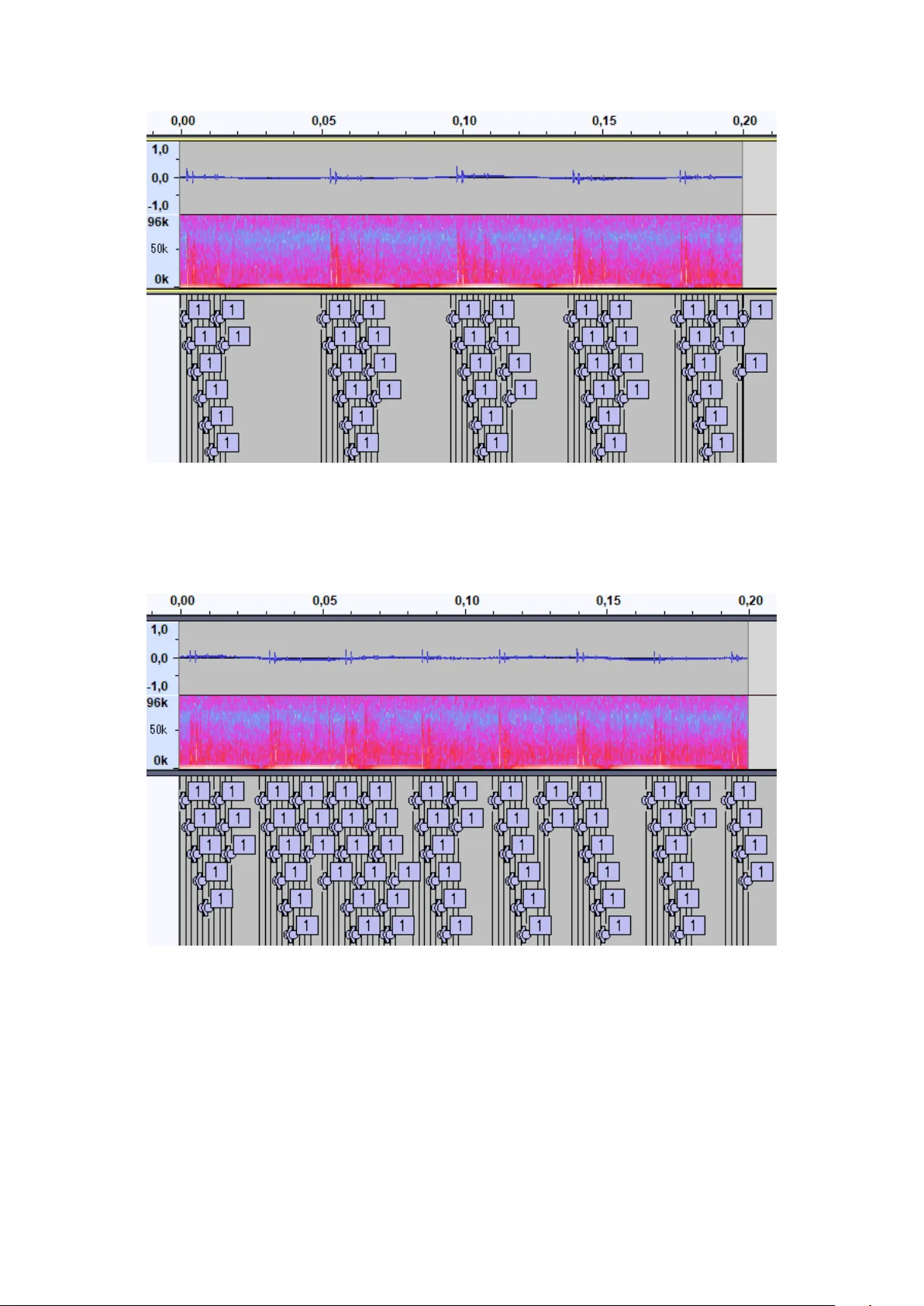
Detection and Classiﬁcation of Cetacean Ec holo cation Clic ks using Image-based Ob ject Detection Metho ds applied to Adv anced W a v elet-based T ransformations Master Thesis Handed in b y: Christopher Hauer Matriculation n um b er: 23110234 First sup ervisor: Alexander Barnhill Second sup ervisor: Prof. Dr.-ing Andreas Maier Advisor: Assistan t Prof. Dr. Heik e V ester Lehrstuhl f ¨ ur Mustererk enn ung (LME) — Martensstr. 3 — 91058 Erlangen — cs5-info@lists.fau.de Decla ration of Originalit y I, Christopher Hauer, studen t registration num b er: 23110234, hereb y conﬁrm that I completed the submitted w ork indep enden tly and without the unauthorized assistance of third parties and without the use of undisclosed and, in particular, unauthorized aids. This work has not b een previously submitted in its current form or in a similar form to an y other examination authorities and has not b een accepted as part of an examination b y an y other examination authorit y . Where the w ording has b een tak en from other p eople’s work or ideas, this has b een prop erly ac kno wledged and referenced. This also applies to drawings, sketc hes, diagrams and sources from the In ternet. In particular, I am a ware that the use of artiﬁcial intelligence is forbidden unless its use as an aid has b een expressly p ermitted b y the examiner. This applies in particular to c hatb ots (esp ecially ChatGPT) and suc h programs in general that can complete the tasks of the examination or parts thereof on m y b ehalf. F urthermore, I am aw are that working with others in one ro om or b y means of so cial media represen ts the unauthorized assistance of third parties within the ab o v e meaning, if group w ork is not expressly p ermitted. Eac h exc hange of information with others during the examination, with the exception of examiners and invigilators, ab out the structure or conten ts of the examination or an y other information such as sources is not p ermitted. The same applies to attempts to do so. An y infringements of the ab ov e rules constitute fraud or attempted fraud and shall lead to the examination b eing graded “fail” (“nic h t b estanden”). 2 Abstract A c hallenge in marine bioacoustic analysis is the detection of animal signals, like calls, whistles and clicks, for b ehavioral studies. Man ual lab eling is to o time-consuming to pro cess suﬃcient data to get reasonable results. Th us, an automatic solution to o v ercome the time-consuming data analysis is necessary . Basic mathematical mo dels can detect even ts in simple en vironmen ts, but they struggle with complex scenarios, lik e diﬀeren tiating signals with a low signal-to-noise ratio or distinguishing clic ks from ec ho es. Deep Learning Neural Netw orks, suc h as ANIMAL-SPOT, are b etter suited for such tasks. DNNs pro cess audio signals as image representations, often using sp ectrograms created by Short-Time F ourier T ransform. Ho w ev er, sp ectrograms hav e limitations due to the uncertain t y principle, whic h creates a tradeoﬀ b etw een time and frequency resolution. Alternativ es like the w av elet, which pro vides b etter time resolution for high frequencies and improv ed frequency resolution for lo w frequencies, may oﬀer adv an tages for feature extraction in complex bioacoustic en vironments. This thesis sho ws the eﬃcacy of CLICK-SPOT on Norw egian Killer whale underw ater recordings pro vided b y the cetacean biologist Dr. V ester. Keyw ords: Bioacoustics, Deep Learning, W a v elet T ransformation 3 Contents 1 Intro duction 6 1.1 Killer Whale V o cal Rep ertoire . . . . . . . . . . . . . . . . . . . . . . . . 6 1.1.1 Killer Whale Calls . . . . . . . . . . . . . . . . . . . . . . . . . . 6 1.1.2 Killer Whale Whistles . . . . . . . . . . . . . . . . . . . . . . . . 6 1.1.3 Killer Whale Clic ks . . . . . . . . . . . . . . . . . . . . . . . . . . 7 1.2 Curren t Situation . . . . . . . . . . . . . . . . . . . . . . . . . . . . . . . 7 1.2.1 Dialog with Dr. Heik e V ester . . . . . . . . . . . . . . . . . . . . 7 1.3 Related W ork . . . . . . . . . . . . . . . . . . . . . . . . . . . . . . . . . 10 1.4 Con tribution . . . . . . . . . . . . . . . . . . . . . . . . . . . . . . . . . . 11 1.5 Ov erview of the next Chapters . . . . . . . . . . . . . . . . . . . . . . . . 13 2 Theo ry 14 2.1 Sound Characteristics of Clic ks, Ec ho es and other Noises . . . . . . . . . 14 2.1.1 Sound Characteristics of Clic ks . . . . . . . . . . . . . . . . . . . 14 2.1.2 Sound Characteristics of Ec ho es . . . . . . . . . . . . . . . . . . . 14 2.1.3 Clic k and Ec ho Diﬀeren tiation . . . . . . . . . . . . . . . . . . . . 15 2.1.4 Other Noises . . . . . . . . . . . . . . . . . . . . . . . . . . . . . 16 2.2 First Order Gradien t Con v ersion . . . . . . . . . . . . . . . . . . . . . . 16 2.3 Sp ectrogram and Phase . . . . . . . . . . . . . . . . . . . . . . . . . . . . 18 2.3.1 F rom the Short Time F ourier T ransformation to the Sp ectrogram 18 2.3.2 The Phase of a Sp ectrogram . . . . . . . . . . . . . . . . . . . . . 19 2.4 W a v elet and Scalogram . . . . . . . . . . . . . . . . . . . . . . . . . . . . 19 2.4.1 The W a v elet . . . . . . . . . . . . . . . . . . . . . . . . . . . . . . 20 2.4.2 Scalogram . . . . . . . . . . . . . . . . . . . . . . . . . . . . . . . 21 2.5 Mac hine Learning . . . . . . . . . . . . . . . . . . . . . . . . . . . . . . . 21 2.5.1 P erceptron . . . . . . . . . . . . . . . . . . . . . . . . . . . . . . . 21 2.5.2 F ully Connected Neural Net w ork Mo del . . . . . . . . . . . . . . 23 2.5.3 2D Con v olutional Neural Net w ork . . . . . . . . . . . . . . . . . . 24 2.5.4 Net w ork T raining . . . . . . . . . . . . . . . . . . . . . . . . . . . 24 2.6 Decision T rees . . . . . . . . . . . . . . . . . . . . . . . . . . . . . . . . . 25 3 Metho dology 27 3.1 Sound Segmen tation using Deep Learning with ANIMAL-SPOT . . . . . 27 3.2 Ob ject Detection for Acoustic Ev en t Recognition with YOLO . . . . . . 28 3.2.1 YOLO P ost Pro cessing using F OD . . . . . . . . . . . . . . . . . 30 3.2.2 Random F orest P ost Pro cessing . . . . . . . . . . . . . . . . . . . 31 4 Data 34 5 Exp eriments and Results 37 5.1 P AMGuard Standalone Exp erimen ts . . . . . . . . . . . . . . . . . . . . 37 5.2 F OD only Exp erimen ts . . . . . . . . . . . . . . . . . . . . . . . . . . . . 38 5.3 ANIMAL-SPOT Exp erimen ts . . . . . . . . . . . . . . . . . . . . . . . . 39 4 5.4 YOLO Exp erimen ts . . . . . . . . . . . . . . . . . . . . . . . . . . . . . . 43 5.4.1 Conﬁdence Threshold Exp erimen ts . . . . . . . . . . . . . . . . . 43 5.4.2 F OD p ost-pro cessing to enhance b ounding b o x p osition . . . . . . 44 5.5 Random F orest Clic k and Ec ho Diﬀeren tiation . . . . . . . . . . . . . . . 46 5.6 Final Optimizations . . . . . . . . . . . . . . . . . . . . . . . . . . . . . . 48 6 Discussion 52 6.1 P AMGuard . . . . . . . . . . . . . . . . . . . . . . . . . . . . . . . . . . 52 6.2 Standalone F OD ev en t detection . . . . . . . . . . . . . . . . . . . . . . . 52 6.3 ANIMAL-SPOT . . . . . . . . . . . . . . . . . . . . . . . . . . . . . . . . 52 6.4 YOLO . . . . . . . . . . . . . . . . . . . . . . . . . . . . . . . . . . . . . 53 6.5 Random F orest . . . . . . . . . . . . . . . . . . . . . . . . . . . . . . . . 53 6.6 Final Optimizations . . . . . . . . . . . . . . . . . . . . . . . . . . . . . . 53 6.7 F uture W ork . . . . . . . . . . . . . . . . . . . . . . . . . . . . . . . . . . 54 7 Summa ry 56 8 Ackno wledgments 58 5 1 Intro duction The ﬁeld of bioacoustics is not just concerned with animal v o calization signal production, but also with their b ehavioral context and intra-species comm unication. T o gather insigh t in to the so cial group b ehavior and dynamics of animals, bioacousticians use data analysis on collected audio data from observed target animals. This analysis helps create hypotheses based on observ ed b ehavior, correlates reo ccurrences of acoustic signals, and predicts the semantic meaning of animal comm unication. T o that regard, one successful starting strategy is trying to map reo ccurring signals to wards a sp eciﬁc animal b ehavior [37], for example, to iden tify mating calls, w arning calls, con tact calls, b egging calls, alarm calls, search calls and more [33]. While this pro cess has b een successful in man y species, such as man y a vian species [34, 51] and mammals [50], the metho d fails in deciphering the con textual meaning from more complex comm unications [22]. One suc h animal sp ecies is the charismatic to othed killer whale ( Or cinus or c a ) [18, 19, 20, 21, 53, 54, 39, 17, 16, 1, 29]. A killer whale vocal rep ertoire has b een catalogued for killer whale p opulations in diﬀerent regions around the world, suc h as the resident p opulation in Canada [18, 19, 20, 21, 17, 16, 41], Iceland [49] and Norwa y [56]. F or similar animals, such as the b ottlenose dolphin, speciﬁc call t yp es lik e signature whistles [30] w ere found. While similar hypotheses w ere put forward on the observ ation of captive killer whales [55], so far, single call t yp es hav e not y et b een assigned to a sp eciﬁc animal b ehavior [58]. The pro cess of deciphering killer whale vocalizations and assigning them to animal behavior is particularly c hallenging because killer whales are p er se hard to observ e. The marine en vironmen t complicates eﬀorts to trac k their b ehavior, and the migratory patterns mak e long-term study virtually impossible. T o gain deep er insigh t in to killer whale comm unication, diﬀeren t approac hes to semantic communication, suc h as call phonetics and turn-taking dialogs and con v ersations could help to determine con text-dep enden t v o calizations. 1.1 Killer Whale V o cal Rep ertoire The v o cal repertoire for killer whales is region-dep endent, as suc h there are diﬀerences b et w een the Canadian call catalog [8], the Icelandic call catalog [49, 25] and the Norwegian call catalog [56]. Y et the underlying structure of the catalog is similar. The killer whale v o calizations are categorized as calls, whistles and clic ks. 1.1.1 Killer Whale Calls Killer whales use stereot yp ed calls for b oth short-range and long-range comm unication [36]. Low-frequency long-range calls can ha v e a p ossible range of 16 kilometers and are more commonly recorded during feeding and foraging. Short-range calls are recorded during so cializing and resting p erio ds and can ha v e a range of up to 9 kilometers. 1.1.2 Killer Whale Whistles Whistles are recorded more often during so cial interaction. As stated, it is susp ected that killer whales use signature whistles for group recognition or kin recognition [55]. 6 Ho w ev er, pro ving the hypothesis is diﬃcult due to the killer whales’ elusive underw ater lifest yle. 1.1.3 Killer Whale Clicks In the o cean, sunligh t decreases rapidly with depth and the visibilit y strongly reduces dep ending on w ater quality and depth [40]. Given these circumstances, to othed whales, suc h as the killer whale, rely on ec holo cation for h unting and na vigation. Echolocation w orks just lik e a biological sonar [48], the killer whale pro duces a p o w erful impulse using its phonic lips in the nasal sacs. The impulse is guided and emitted through the melon, a round-shap ed organ in the killer whale’s forehead which consists of fat. The melon acts lik e an acoustical lens to focus the clic ks in to a directional b eam. The returning ec ho is captured by the fat-ﬁlled ca vities in the lo wer jar b one and received in the auditory bulla. During na vigation or h un ting, the killer whale can emit hundreds of clicks in rapid succession, known as a click train or burst, to target sp eciﬁc areas of interest or gather con tin uous information about their prey [28]. Ho wev er, it is also suspected that clic ks could pla y a role in comm unication. 1.2 Current Situation T o b etter understand the killer whale’s use of clic ks, they should b e analyzed in con text to determine whether they serv e a comm unicativ e purp ose. T o do this, the clic ks need to b e detected and annotated, which can p ose n umerous problems. The most common problem is that b oth the killer whale clicks and the returning echoes are recorded. As ec ho es are reﬂected clic ks from surfaces, suc h as the o cean ﬂo or and the water surface, they share man y characteristics with their original clic k. Since ec ho es are dep enden t on the en vironment, they should b e diﬀerentiated from the clicks for b etter quantiﬁable measuremen ts. Y et, the diﬀerentiation b etw een clic ks and ec ho es is diﬃcult, as the v ersatilit y of clicks in diﬀeren t environmen ts and the similarit y b etw een clic ks and ec ho es mak es it diﬃcult to diﬀeren tiate the t wo in isolation. The six images in Figure 1 sho w some examples of the diﬀeren t clicks and echoes encoun tered in the ﬁeld from diﬀeren t signal-to-noise ratio (SNR) en vironmen ts. 1.2.1 Dialog with Dr. Heike V ester T o understand the problem with detecting and annotating clic ks, Dr. Heik e V ester, a biologist who sp ecializes in the so cial b ehavior and bioacoustic of marine mammals, w as in terview ed to share her exp eriences with detecting and hand labeling clic ks from the Norw egian killer whale p opulation. Stationed in Bo dø, Norwa y , she is the founder of Ocean Sounds e.V. [15] and provided b oth the task and the data for this master thesis. F ollo wing is a repro duced summary of the interview with Dr. V ester at the Ocean Sounds studio. 1. Ho w is the data collected? The data are only collected when the orca is visible and iden tiﬁed via PhotoID. A matriline can b e iden tiﬁed b y its mem b ers, whic h can b e identiﬁed b y their saddle 7 (a) W a v eform and sp ectrogram of a high SNR clic k (b) W a v eform and sp ectrogram of a medium SNR clic k (c) W a v eform and sp ectrogram of a lo w SNR clic k (d) W a v eform and sp ectrogram of a high SNR ec ho (e) W a v eform and sp ectrogram of a medium SNR ec ho (f ) W av eform and sp ectrogram of a lo w SNR ec ho Figure 1: Six example images of the w a v eform and sp ectrogram of diﬀeren t clic ks and ec ho es in isolation. The diﬀering SNR v alues can happ en due to the distance of the emitted clic k to the h ydrophone and the directionalit y of clic ks. The sp ectrogram w as generated with a segmen t size of 16 samples and a hop of 8 samples. The n um b er of samples are v ery lo w when compared to the more commonly used 1024 segmen t size and 512 hop. This is necessary due to the small windo w size of only 384 samples (2 milliseconds using 192kHz). This explanation also holds for other pictures. patc h and ﬁn. A single h ydrophone with a sampling rate of 192 kHz is lo w ered from the b oat to record the animals. In addition, the animals’ b eha vior during the recording is noted [56]. 2. Wh y are clic ks so n umerous and imp ortan t? Killer whales primarily use ec holo cation to b oth orien t themselv es and to ﬁnd and trac k prey during a hun t. But clicks are also emitted n umerously during so cial in teractions. Observing more animals, like during so cial interaction, will gain more clic ks than observing a single group with fewer animals, of course. But the purp ose of clic ks during so cial in teractions, where the animals can visually see eac h other, remains a mystery . A quantiﬁable analysis of clic ks could help to decipher the meaning and usage of clic ks for killer whales in situations where it migh t not b e necessarily used for ec holo cation alone. 8 3. Ho w are the data hand lab eled? The data is hand lab eled using Audacity [52]. By searching through the wa veform of a signal to ﬁnd high-frequency Dirac-lik e impulses or energy-ric h impulses. These impulses, which span through the entire bandwidth, can also b e found in the sp ectrogram. The ev en ts are marked with text annotations using a separate lab el trac k. 4. Ho w can one tell clic ks and ec ho es apart from eac h other? Clic ks and ec ho es are diﬀeren tiated through the con text of the ev ent. Lo oking at an individual impulse usually do es not pro vide enough information. The killer whales emit bursts of clic ks to generate an image of their surrounding. These clic ks are generated in somewhat equidistan t time in terv als. Of course, they are not exactly equidistan t, these bursts can sp eed up and slow do wn in ev en t frequency when the killer whale zo oms into an area of interest. Strong and obvious clic ks and ec ho es can b e told apart b y their diﬀeren t phases, a clic k usually starts with a p ositiv e amplitude, an ec ho with an in v erted negative phase, but that is not alw ays the case as can b e seen in Figure 2. The robust wa y of distinguishing clic ks and ec ho es is b y comparing the impulse with their neigh b oring patterns. F or instance, if the time in terv als are roughly equidistan t, like in a burst, or if the click is signiﬁcantly more in tense than the echo, distinguishing b et w een them becomes easy , as can be seen in Figure 3. If a clic k is weak er or does not follow the burst structure, then it is more diﬃcult to distinguish, in those cases, it tak es some exp erience and in tuition to diﬀeren tiate b et w een clic ks and ec ho es. 5. What types of lab els are used? The obvious clic ks are divided into three subtypes based on their p eak (most energy) frequency range in the sp ectrogram. If a click has a peak b elow 5 kHz, it is lab eled as a low-frequency (LF) clic k. If it has a peak b etw een 5 kHz and 40 kHz, it is lab eled as a high-frequency (HF) clic k. In the case of a p eak abov e 40 kHz, the clic k is lab eled as an ultrasonic-frequency (US) click. Figure 4 sho ws the three diﬀerent lab eled clicks. In comparison to LF and HF clic ks, US clicks are rare. Sometimes it is diﬃcult to determine the max energy in w eak er clic ks, which do not ha v e a lot of energy and are barely visible in the spectrogram and time signal. These w eak clicks are sometimes annotated with a suggestion on what the frequency could probably b e, lik e w eak LF clic ks. Since the echoes are less critical to the analysis, they are not diﬀeren tiated b y p eak frequency and are simply lab eled as ec ho es. 6. Are there problems with the hand lab eling? The biggest problem is time. During a burst, a killer whale can emit more than a h undred clic ks in less than a second. These clicks can ha v e m ultiple ec ho es, so it is p ossible to hav e hundreds of even ts in a single second. Assuming it tak es an exp erienced bioacoustician ten seconds to lo cate, mark, and compare an ev en t with its surrounding con text to create a lab el, the task b ecomes signiﬁcan tly more time-consuming when there are m ultiple even ts to lab el. F or instance, if a burst con tains 150 clic ks and 210 echoes within a single second, the bioacoustician would need approximately one hour to lab el just that one second of data. Of course, not 9 ev ery second of the data material con tains a burst. Ho w ever, it to ok t welv e hours to label a single min ute of data material. This is just not sustainable for a goo d data analysis, ev en with the help of a team. 7. F or a start, w ould an ev en t detector help in sp eeding up the analysis? If an even t detector can ﬁnd and pre-mark the clic ks and echoes, then that could help, but it w ould not solv e the actual problem. The lab eling of the ev en t still tak es a signiﬁcan tly long time. Ev en if the annotation pro cess could b e accelerated to b e t wice as fast, taking six hours to lab el just one min ute of data is still unsustainable for thorough data analysis. This task demands a fully automated solution. 8. Giv en the problem, there is a high probabilit y that the mac hine would not b e as reliable as an exp erienced biologist. What w ould b e a go o d compromise? The ﬁrst goal is to quan tify the click occurrences and correlate them to animal b eha vior, so that w e predict their b eha vior in the future without the need to see the animals, e.g. feeding ev en ts versus so cializing or trav eling. T o ac hiev e this, the clic ks need to b e compared with the animal’s activity and b ehavior. How ever, the pro cess does not need to b e ﬂa wless from the outset. F or instance, if the mac hine is accurate in 90% of the cases, the results can still b e used for further analysis. 9. Concerning true p ositiv e, false p ositiv e, true negativ e, false negative cases, what should b e the fo cus? The fully automated solution should maximize the ov erall accuracy . If a compromise exists b et w een missing click edge cases and minimizing false p ositive ﬁndings, then the focus should be on minimizing the total n um b er of errors b et w een both false p ositiv e and false negativ e cases. 10. Human in tuition is diﬃcult to deﬁne, what features could b e used for clic k and ec ho diﬀeren tiation? Assuming that the ev en t detection is working, the in ter-arriv al-time b et w een ev en ts, the energy densit y and max energy as well as the starting phase could b e useful features for distinguishing clic ks and echoes. These w ould need to be compared b et w een multiple ev ents to get the bigger picture. Of course, the maxim um energy o v er the frequency is needed for the LF, HF and US diﬀeren tiation. 1.3 Related Wo rk Bioacoustic click ev en t detection is not a new ﬁeld of study . There are many bioacoustic to olkits whic h provide click detectors for passiv e acoustic monitoring based on diﬀeren t approac hes. SEDNA [12], developed b y the Bioacoustic Researc h Program at Cornell Univ ersit y and the Lab of Ornithology , pro vides a bioacoustic click detector based on MA TLAB to ols for the use of environmen tal impact assessmen t. The work of C. Gerv aise et al. [24] uses a click detector based on the kurtosis of a signal to researc h the psyc hological impact of noise p ollution. T o the b est of the author’s kno wledge, the most widely used op en-source click detector would b e the P AMGuard clic k detector [42], 10 (a) W a v eform and sp ectrogram of a common clic k and ec ho pair (b) W a v eform and sp ectrogram of a pair with the same starting amplitude (c) W a v eform and sp ectrogram of a pair with in v erted starting amplitude Figure 2: Three example images of clic k and ec ho pairs. Image (a) sho ws a usual clic k and ec ho pair, with a p ositiv e starting amplitude clic k and a negativ e starting amplitude ec ho. Due to a w eak initial phase, the ec ho in image (b) app ears to ha v e a p ositiv e starting amplitude. In Image (c), due to the strong impulse compared to the initial amplitude, it lo oks lik e the clic k starts with a negativ e amplitude and ec ho with a p ositiv e amplitude. dev elop ed by Jamie Macaula y , Doug Gillespie and Mic hael Oswald. The P AMGuard clic k detector is based on Ja v a and uses energy o ver frequency thresholds to ﬁnd clicks. Another approach for calls rather than clic ks is ANIMAL-SPOT [3], a ResNet18-based Con v olutional Neural Netw ork (CNN) that p erforms detection segmentation using a sliding window approach. The ANIMAL-SPOT mo del has b een a ma jor inﬂuence on the developmen t of this thesis. The tw o w orks of Berman t et al. [4, 5] provide mac hine learning to ols to ﬁnd and annotate clic ks and codas of sp erm whales. The ﬁrst machine learning techniques were based on Con v olutional Neural Netw orks (CNNs) to extract ﬁner-scale details from cetacean sp ectrograms [4]. The later work pro vided a self-sup ervised deep learning metho d which uses Noise Contrastiv e Estimation to ﬁnd sp ectral changes [5]. The Listening-Lab Annotator developed by McEw en et al. [35] utilizes a w a v elet-based segmen tation metho d that automatically extracts transient features. Ho w ev er, the approach still relies on h uman-in-the-lo op in terven tion for classiﬁcation. This work has signiﬁcantly inﬂuenced the developmen t of this thesis, serving as a k ey inspiration for the metho dology emplo y ed here. 1.4 Contribution Man y of the bioacoustic click detectors in passive acoustic monitoring use threshold-based baseline metho ds, whic h do not p erform well in environmen ts with a lo w signal-to-noise (SNR) ratio or do not p erform adequate clic k ec ho diﬀerentiation without the need for h uman correction. This thesis fo cuses on the detection and diﬀeren tiation of killer whale clic ks and ec ho es to dev elop an even t detector capable of iden tifying both clicks and ec ho es, along with implementing a metho d for distinguishing b etw een the tw o. T o ac hiev e this, several approac hes were tested, utilizing wa veform, sp ectrogram, and 11 Figure 3: An example of the w a v eform, sp ectrogram and lab els in Audacit y . The equidistan t clic k ec ho pairs mark ed within green b o xes are part of a burst. The clic k and ec ho pairs mark ed with orange b o xes are also easy to distinguish, but not part of the same burst as the ones mark ed with green. The ev en ts mark ed with red b o xes are lab eled, but diﬃcult to iden tify and p oten tially wrong. scalogram audio represen tations in conjunction with ANIMAL-SPOT and YOLO mo dels. In this w ork, the to ol-chain CLICK-SPOT is introduced. CLICK-SPOT is enhancing a YOLO mo del with a First order detection (F OD) p ost processor and a random forest con text classiﬁer to ﬁnd, annotate and label clic k and ec ho es from an audio ﬁle of an underw ater recording. CLICK-SPOT was dev elop ed in three stages, the ﬁrst alpha v ersion only consisted of the YOLO mo del and merged b ounding b o xes. The second b eta v ersion added the FOD p ost processor to enhance the b ounding boxes. The ﬁnal CLICK-SPOT v ersion added a random forest con text classiﬁer to diﬀeren tiate clic ks from ec ho es. Although these to ols are sp eciﬁcally designed for detecting killer whale clic ks and ec ho es, many of the metho ds and mo dels can b e adapted for iden tifying target signals of other animal sp ecies as w ell. 12 (a) Lo w-F requency (LF) clic k (b) High-F requency (HF) clic k (c) Ultrasonic-F requency (US) clic k Figure 4: Example of a lo w-frequency clic k [image (a)], a high-frequency clic k [image (b)] and an ultrasonic-frequency clic k [image (c)]. 1.5 Overview of the next Chapters The follo wing chapters are structured as follo ws. In the theory c hapter, the underlying theory for ANIMAL-SPOT and YOLO are describ ed and summarized. The metho dology pro vides an o verview of the ANIMAL-SPOT and YOLO mo dels, as well as the context approac h used in the exp eriments and results. The Data chapter pro vides a description of the data pro vided b y Dr. V ester from Ocean Sounds, as well as its usage and prepro cessing for ANIMAL-SPOT and YOLO training. The exp erimen ts c hapter describ es the exp eriments performed in this thesis and rep orts on the results achiev ed in the exp eriments. The discussion chapter explains what problems occurred during the exp erimen ts, what could b e learned from the exp erimen t, and what problems o ccurred during the exp erimen ts. The conclusion summarizes this thesis and giv es a further outlook on what could b e done in the future. 13 2 Theo ry This chapter will give a summary of all the theories necessary to describ e the task and metho dology used in this thesis. It will ﬁrst start with the physical attributes of clic ks, ec ho es and the surrounding noise in underwater bioacoustics b efore diving into the tec hnical asp ects of First Order Detection (F OD), ANIMAL-SPOT, YOLO and con text-dep enden t analysis. 2.1 Sound Characteristics of Clicks, Echo es and other Noises Sound trav els faster underw ater (appro ximately 1500 m/s ) than through the air (appro ximately 343 m/s ). While there are diﬀerences in tra v el time and distance atten uation b et w een underwater and air acoustics, the underlying theory remains the same for b oth systems. T o understand the problems and challenges in the follo wing c hapters, the attributes of orca clicks and ec ho es as well as other noises ha v e to b e analyzed and explored ﬁrst. 2.1.1 Sound Characteristics of Clicks A click is a Dirac-like impulse, typically starting with a p ositiv e amplitude. As stated in the introduction, the killer whale emits these clic ks, which usually feature low-frequency (LF) p eaks b et w een 20 Hz and 5 kHz, high-frequency (HF) p eaks b etw een 5 kHz and 40 kHz [27], or ultrasonic-frequency (US) peaks ov er 40 kHz. US clic ks are less commonly observ ed compared to LF and HF clicks. This ma y be due to the shorter transmission range of higher-frequency sounds underw ater, coupled with the greater directionalit y of these clicks, making them less lik ely to be recorded. Alternativ ely , it could simply b e that these clicks are used less frequen tly in vocalizations. Examples of these clicks can b e seen in Figure 4. The energy intensit y of a killer whale clic k is diﬃcult to estimate [27] due to the directional beam forming and high v ariation. The killer whale can produce clic ks with a strength similar to that of the sp erm whale, ranging from 188 decib els (dB) to p ossibly as high as 230 dB. F rom measurements of the pro vided data, on a verage, a killer whale click lasts less than 1 millisecond, and the in ter-arriv al time b etw een clicks in a burst can be shorter than 2 milliseconds. The click t ypically b egins with a positive amplitude impulse, but due to the underlying electrical noise ﬂo or and electrical system noise, determining the starting amplitude b ecomes c hallenging for clic ks emitted far a wa y from the h ydrophone. The noise can distort the signal and aﬀect b oth the minim um and maxim um energy spikes. As a result, the prominent energy spik es are, while still useful, not fully reliable indicators for distinguishing b et w een clic ks and ec ho es. 2.1.2 Sound Characteristics of Echo es Ec ho es are b ounced reﬂections of the clic k from a surface. F rom the pro vided data it can b e seen that the echoes can arriv e an ywhere betw een less than a millisecond and 20 or more milliseconds dep endent on the underw ater tra vel time. On a v erage, surface reﬂected ec ho es arriv e 1.5 milliseconds after the click. V ariations in click ec ho interarriv al time can also b e seen in Figure 2. The ec ho exhibits a similar structure to the click but with 14 an in verted starting amplitude. Both clic ks and ec ho es exp erience atten uation as they tra v el through w ater, causing rev erb eration eﬀects. The p eak frequency of the ec ho can shift b y 0.1 kHz to 2 kHz, inﬂuenced b y factors suc h as the angle and prop erties of the reﬂectiv e surface. These rev erb erations complicate the precise identiﬁcation of the echo’s start and end p oin ts, as can b e seen in Figure 5a. (a) An example of a clic k and ec ho pair. The ec ho is more diﬃcult to determine due to rev erb erations. (b) An example of a clic k and ec ho pair. Due to the frequency shift of the ec ho and rev erb eration, the energy in certain bands can b e higher than the original clic k, leading to a higher p eak and/or a v erage energy in the ec ho rather than the clic k. Figure 5: Examples of a rev erb erated ec ho in image (a) and a frequency shifted rev erb erated ec ho in image (b). The ec ho in image (b) has a higher p eak and a v erage energy than the clic k. In terestingly , due to frequency shifts and p oten tial o verlap with underlying noise, the ec ho can hav e a higher p eak and/or av erage energy than the clic k. One example of such an o ccurrence of a clic k and echo pair with a stronger ec ho can b e seen in Figure 5b. That means that the maxim um and a verage energy alone are unreliable indicators for diﬀeren tiating b et w een clic k and ec ho. 2.1.3 Click and Echo Diﬀerentiation When seen as a pair, diﬀerences from attenuation and reverberation are apparen t, as can b e seen in Figures 2 and 3. Y et, when lo oked at in isolation, the clicks and echoes are to o v ariable, as can b e seen in Figure 1. F eatures like p eak and av erage energy , phase, and structure alone are insuﬃcient for diﬀerentiation b et w een clicks and ec ho es. T o ac hiev e accurate diﬀeren tiation b et w een clic ks and ec ho es, these characteristics should be 15 analyzed in conjunction with other metrics, such as context information like inter-arriv al times, as w ell as the diﬀerences in p eak v alues, a v erages, and the structural patterns of m ultiple ev en ts. 2.1.4 Other Noises Unfortunately , pulsed Dirac-like impulses, suc h as clicks, are common in nature. After all, the killer whale is not the only whale that uses ec holo cation. In addition, other sources suc h as raindrops, b oat noises, or technical interferences like mechanical or electrical noise can also pro duce diﬀeren t Dirac-like impulses which aren’t alwa ys pulsed, but are still similar enough to be diﬃcult to discern from clic ks as can be seen in Figure 6. These in terferences can be a challenge, when distinguishing those from killer whale (a) W a v eform and sp ectrogram of an in terference (b) W a v eform and sp ectrogram of a dolphin clic k (c) W a v eform and sp ectrogram of a pilot whale clic k Figure 6: Three examples of p ossible noises. Image (a) sho ws mec hanical or electrical in terference. Image (b) depicts a clic k and echo pair from a dolphin, image (c) from a pilot whale. clic ks, esp ecially when the even ts are rev erb erated and attenuated. Consequently , simple mathematical assumptions are insuﬃcient for reliable diﬀerentiation b etw een clicks, ec ho es and noise in suc h complex underw ater en vironmen ts. 2.2 First Order Gradient Conversion As clic ks and echoes are Dirac-like in nature, they usually p ossess a steep er gradient in comparison to their surroundings. As suc h, the gradien t of an audio signal could b e used as a go o d feature for click and ec ho ev en t detection. The ﬁrst order gradient conv ersion can b e used to transform the signal into its gradien t representation b y subtracting a v alue from its previous v alue. It is identical to the ﬁrst step of the contin uous w a v elet transformation of the Haar wa velet. The ﬁrst-order gradien t con v ersion does not provide a clean transformation of the signal. T o eﬀectiv ely extract the gradient p eaks, it is necessary to remo v e the noise. Ho w ev er, due to factors suc h as distance, reverberation, 16 (a) The original signal represen ted in its w a v eform and sp ectrogram. (b) The ﬁrst order gradien t con v erted signal. The sp ectrogram shows that a lot of noise is still presen t in b et w een the gradien t p eaks. (c) Mo ving a v erage. The lo cal gradien t a v erage o v er 1000 samples for ev ery sample. (d) Noise reduction. The mo ving a v erage and samples are calculated against a threshold function. Figure 7: This ﬁgure w as generated using Audacit y . It displa ys the pro cess of the ﬁrst order Dirac-lik e impulse detection (F OD). Image (a) sho ws an example of an original signal. Image (b) displa ys the absolute v alues of the ﬁrst order of the signal. Image (c) is a moving a v erage ov er the signal, which is used to increase or reduce a threshold function. Image (d) sho ws the noise-reduced Dirac-lik e remains of the absolute v alues of the ﬁrst order signal. Some of the remains are so short that they do not app ear on the sp ectrogram. and atten uation, a simple threshold is insuﬃcien t for eﬀective noise suppression. Instead, the lo cal mean energy ﬂuctuations of the signal m ust b e considered when determining the noise remov al threshold. T o account for this, a mo ving a verage function ov er 1000 lo cal gradien ts w as applied. The noise reduction equation: N r ( s ) =  s for s ≥ 8 m 2 + 2 . 4 m + 0 . 024 0 for s < 8 m 2 + 2 . 4 m + 0 . 024 (1) Nr(s) represents the noise-reduced gradien t sample, where s is the gradient sample of the con v erted signal, and m is the lo cal mo ving a v erage of the sample (calculated o ver 1000 samples). This equation was derived b y ﬁtting a curve to a test dataset, and it applies to the ﬁrst-order noise-reduced Dirac-lik e impulse detector (F OD). Using the noise reduction equation, the mo ving av erage and the gradient of the signal are calculated against a 17 threshold function to transform the gradient signal into a noise-reduced Dirac-lik e impulse p eak represen tation. This pro cess can b e seen in Figure 7. The ﬁrst order gradien t can also b e padded to gain the gradien t for lo w er frequencies. In this work, only the unpadded ﬁrst order gradien t con v ersion is used. This application of the F OD can also b e used as a standalone detector. 2.3 Sp ectrogram and Phase The sp ectrogram [38] is one of the most widely used visual represen tations of audio signals. It is derived from the Short-Time F ourier T ransform (STFT), whic h analyzes the signal in small, o v erlapping time segmen ts. 2.3.1 From the Sho rt Time F ourier T ransfo rmation to the Spectrogram The STFT performs sp ectral analysis on a time windo w of the target signal [38]. The windo w size is typically a p o w er of 2, whic h corresp onds to the n um b er of frequency bins, represen ting the num b er of o v erlapping sinusoidal wa ves used to approximate the signal inside the time window. The STFT calculates tw o components for eac h frequency bin, the in-phase comp onen t and the out-of-phase comp onen t. These are returned as a complex n um b er, with the in-phase comp onen t corresp onding to the real part and the out-of-phase comp onen t corresponding to the imaginary part. By com bining b oth components, w e can calculate the magnitude, whic h represents the strength (as in amplitude) of the signal as the absolute v alue of the complex num b er, and the phase, which corresp onds to the angle betw een the real and imaginary comp onents. The magnitude is represented as a one-dimensional array of amplitudes across the frequency bins, reﬂecting the frequency sp ectrum of the signal. This array can then b e transformed into a 1D pixel array , represen ting the time window. This pro cess of generating 1D pixel arra ys is repeated m ultiple times by shifting the window with a hop ov er the signal. F or eac h windo w, a new 1D pixel arra y is generated, whic h are com bined in to a 2D image, whic h is kno wn as the sp ectrogram. The Uncertaint y Principle The uncertaint y principle concerning the sp ectrogram states that either a high-frequency resolution or a high time resolution can be ac hiev ed, dep ending on the windo w size, but not b oth simultaneously . A larger windo w provides more frequency bins, resulting in higher frequency resolution. Ho w ev er, the larger windo w also blurs the time resolution. Conv ersely , a smaller windo w size oﬀers a b etter time resolution, but b ecause it allows for few er frequency bins, the frequency resolution decreases. This problem is depicted in Figure 8. It is p ossible to in terp olate v alues in b oth the time and frequency domain to generate additional pixels, but this interpolation do es not improv e the resolution. Another option for generating more pixels in the time domain is to reduce the hop size. How ever, a larger windo w will still blur the time resolution o ver multiple pixels, ev en with a smaller hop size. The choice of windo w size is t ypically a trade-oﬀ b etw een frequency and time resolution, dep ending on the sp eciﬁc task at hand. F or example, in the case of a Dirac-like click sound, which is a brief signal that spans the entire frequency range, time resolution b ecomes more imp ortan t 18 than frequency resolution. If time resolution is blurred, it could b e diﬃcult to accurately pinp oin t the start and end of the signal. (a) W a v eform and sp ectrogram with windo w size 64 samples (0.3 Milliseconds). (b) W a v eform and sp ectrogram with windo w size 128 samples (0.7 Milliseconds). (c) W a v eform and sp ectrogram with windo w size 256 samples (1.3 Milliseconds). Figure 8: Three examples of the same clic k and ec ho with diﬀeren t sp ectrogram windo w sizes. Image (a) shows the w a v eform and sp ectrogram of a signal with an FFT windo w size of 64. With this windo w size, the clic k and ec ho can still b e distinguished, although there is a p o or tradeoﬀ b et w een frequency and time resolution. Image (b) uses a windo w size of 128 samples. With this larger windo w, it b ecomes diﬃcult to diﬀeren tiate b et w een the clic k and the ec ho, and pinp oin ting their exact start or end is challenging. Finally , Image (c) uses a windo w size of 256 samples, where the clic k and ec ho ha v e merged due to the reduced time resolution, th us making them indistinguishable. 2.3.2 The Phase of a Sp ectrogram The phase is the angle b et w een the real and the complex part of the sp ectrogram. It pro vides further information on the angle of the w a v eform, which, in addition to the amplitudes of the sp ectrogram, can b e used so that the unique w a v e co eﬃcien ts can b e reconstructed. 2.4 W avelet and Scalogram The w av elet transformation [6, 10] is similar to ﬁlter transformations, suc h as Gaussian or Laplace ﬁlters. Ev en though m ultidimensional wa v elets exist, this work fo cuses solely on one-dimensional audio signal streams to generate a 2D image representation also known as a scalogram. Therefore, in this thesis only one-dimensional w a v elet transformations are discussed. 19 2.4.1 The Wavelet Unlik e the inﬁnite sin usoidal ﬁlters used in the STFT transformation, w a v elet ﬁlters are ﬁnite in length. A w av elet can b e though t of as a window function that transforms a signal in to a ﬁltered representation using the Con tin uous W av elet T ransform (CWT) function. Typically , the windo w is shifted b y one sample at a time, which ensures that the ﬁltered representation has the same sample size as the original signal. By increasing the window size, the resulting represen tation b ecomes smaller. There are several t yp es of wa velets, such as the Haar w a v elet, Mexican Hat w a v elet, Meyer w a v elet, and Morlet w a v elet, to name a few. The Haar w a v elet and Mexican Hat wa velet are b oth depicted in Figure 9. In this w ork, after careful consideration, the Mexican Hat w a v elet was c hosen for the CWT function to transform the signal. This decision w as based on the fact that the Mexican Hat is a compact and symmetrical wa velet which p erforms the second order con v ersion, making it particularly eﬀectiv e for detecting higher frequency c hanges. (a) The discon tin uous, unsymmetrical Haar w a v elet. (b) The con tin uous, symmetrical Mexican Hat w a v elet. Figure 9: Examples of w a v elets tak en from Wikip edia [59] The ﬁrst step of the Haar con tin uous w a v elet transformation of image (a) w as used for the ﬁrst order gradien t con v ersion and ﬁrst order Dirac-lik e ev en t detection (F OD). The Mexican Hat wa velet from image (b) w as used to generate the scalogram. The Mexican Hat is the smallest symmetrical w a v elet in terms of used samples. Scaling A single wa velet transformation is not enough to transform the signal into a 2D represen tation. The windo w size of a w a v elet corresp onds to the frequency range it represents. By increasing the windo w size, the frequency range co v ered b y the transformation c hanges. The window size of a wa velet can be adjusted through scaling. Eac h scaled version of the wa velet represents a diﬀeren t frequency range, and eac h v ersion corresp onds to a pixel on the scalogram. Scaling the wa velet also aﬀects the time-frequency resolution. A smaller w a v elet window pro vides lo w-frequency resolution 20 but high time resolution for high frequencies, while a larger windo w oﬀers a high frequency resolution for lo w frequencies but lo w er time resolution. 2.4.2 Scalogram By stac king the scaled w av elet transformations, a 2D image representation of the signal is generated based on the scaled wa velets. An example of a scalogram is depicted in Figure 10. The frequency axis follows a logarithmic distribution, where higher frequencies hav e high time resolution and lo w er frequencies ha v e high-frequency resolution. The main adv an tage of the scalogram, compared to the spectrogram, is that Dirac-lik e impulses are b etter visualized at high frequencies, and the scalogram also pro vides a denoising eﬀect. How ever, similar to the spectrogram, the phase information is lost in the wa velet represen tation. Overall, the denoising eﬀect and high-frequency time resolution make the scalogram particularly useful for a deep learning-based clic k detector. In order to impro v e p erformance, the scalogram w as built using 20 v alues from a geom space b etw een 1 and 50. This means that the scalogram represents a frequency range b et w een 960 Hz and 48 kHz. This means that frequencies higher than 48 kHz are not depicted. Y et, the gradient energy of higher frequencies are still presen t in the scalogram in lo w er frequencies. They lo ok lik e protruding double cones that appear from the top of the scalogram, as can b e seen in Figure 10. 2.5 Machine Learning With the adven t of more p ow erful computers, increasingly complex tasks can b e tackled. Ho w ev er, these tasks often cannot be fully deﬁned through mathematical assumptions alone. This is where supervised machine learning comes in, allo wing algorithms to improv e b y learning from prior experiences. I n sup ervised learning, the training data is pre-lab eled with a ground truth lab el, enabling a direct comparison b etw een the mo del’s predictions and the annotated results. This section provides an o v erview of the k ey comp onents of deep neural netw orks and supervised mac hine learning, la ying the foundation for a clearer understanding of the netw orks and mo dels presented in the subsequen t metho dology c hapter. 2.5.1 Perceptron The p erceptron [46] is a fundamen tal building blo c k of neural net w orks and consists of four k ey comp onen ts: the input, trainable w eights, a non-linear activ ation function, and the output. In operation, each input X is m ultiplied b y its corresponding trainable w eight W. The sum of these weigh ted inputs is then passed through an activ ation function to compute the p erceptron’s output. A depiction of the Rosen blatt p erceptron can b e seen in Figure 11. The activ ation function must be non-linear. Otherwise, a stack of p erceptrons could b e reduced to a single matrix-matrix m ultiplication, whic h would limit the mo del’s abilit y to solv e more complex tasks. Common examples of non-linear activ ation functions include the binary step, sigmoid, tanh, and the Rectiﬁed Linear Unit (ReLU), along with v arian ts such as leaky ReLU, Exp onential Linear Units (ELU), and softmax, among others. Depictions of the Sigmoid, T anh and ReLU can b e seen in Figure 12. 21 Figure 10: An example of a Scalogram with its resp ectiv e w a v eform. The Dirac-lik e impulses can b e easily seen and trac k ed as the outlying cones protruding from the top of the image. The represen tation can b e particularly useful for a clic k detector. Figure 11: A visual represen tation of the Rosen blatt p erceptron using TikZ [9]. The inputs X are m ultiplied b y their corresp onding trainable w eigh ts W, and the w eigh ted sum is calculated. This sum is then passed through an activ ation function to pro duce the ﬁnal output. 22 (a) Sigmoid activ ation function (b) T anh activ ation function (c) ReLU activ ation function Figure 12: Depiction of the Sigmoid(a), T anh(b) and ReLU(c) activ ation functions tak en from Wikip edia. 2.5.2 Fully Connected Neural Net w o rk Mo del A neural netw ork is a mo del made up of stac k ed p erceptron lay ers. In a fully connected neural net w ork, ev ery output from a previous la y er is connected to the input of eac h p erceptron in the following la y er. A mo del depiction of a fully connected neural netw ork can b e seen in Figure 13. The netw ork learns by adjusting the p erceptron weigh ts during Figure 13: A depiction of a small fully connected deep neural net w ork tak en from stac k exc hange [23], where ev ery output from a previous la y er is connected to the input of eac h p erceptron in the follo wing la y er. training to minimize the error b etw een the predicted and the annotated outputs ov er m ultiple examples. 23 2.5.3 2D Convolutional Neural Net wo rk A fully connected neural netw ork p erforms optimally when the inputs are indep endent of eac h other. Ho wev er, this is not alw a ys the case. In images, pixels that are close together are more lik ely to b e related to a common shap e than those that are farther apart. In suc h scenarios, conv olutional neural net w orks (CNNs) are designed to exploit the spatial lo calit y of data to extract meaningful features. While con volutions can exist in higher dimensions, this thesis fo cuses on 2D con v olutions for image pro cessing. A 2D conv olution Figure 14: Depiction of a 2D con v olution with a stride of 1 and no padding. The original 6x6 image is pro cessed in to a smaller 4x4 represen tation using a 3x3 k ernel. The image w as tak en from zaforf GitHub [60]. is a t yp e of p erceptron where the inputs are arranged into a ﬁlter, t ypically a square ﬁlter suc h as 3x3, 5x5, or 7x7. These trainable ﬁlters help generate a new representation of the original image based on the p erceptron’s learned weigh ts. Figure 14 depicts ho w a 2D con v olution transforms an image in to a feature map represen tation. Additionally , these conv olutional ﬁlters can b e stack ed, allowing subsequen t 2D conv olutions in deep er la y ers to op erate on the feature maps generated b y earlier la yers, as depicted in Figure 15. Moreov er, con v olution can b e used to reduce the spatial dimensions b y increasing the hop or stride of the image while preserving the essen tial features and relev ant information extracted b y the ﬁlters. 2.5.4 Netw o rk T raining Sup ervised training of a neural net w ork typically requires three datasets comprised of annotated data. A training dataset, a v alidation dataset and a test dataset. The training dataset is used to iterativ ely impro v e the netw ork in tw o steps. First, the training data is fed into the net w ork to calculate an output. This output is then compared to the exp ected output of the training data, kno wn as the lab el, to calculate the loss of the netw ork on the sample. In the second step, a small learning rate is used to backpropagate the loss through the net w ork. This pro cess adjusts the trainable weigh ts, bringing the output closer to the 24 Figure 15: Depiction of a t ypical deep CNN mo del. In the ﬁrst la y er, the original image is transformed into m ultiple represen tativ e feature maps, every feature map is a con v olution of the original image o v er a k ernel ﬁlter. This step is rep eated iterativ ely , the subsequen t 2D con v olutions in deep er la y ers are stac k ed on the feature maps generated b y earlier lay ers until the feature map is ﬂattened in to a 1D arra y and further pro cessed using a fully connected neural net w ork. The image w as tak en from P ark explanation of CNN mo dels[26]. exp ected v alue. These steps are rep eated o ver m ultiple iterations of the entire training set, also kno wn as an ep o ch, to reﬁne the netw ork’s p erformance. The v alidation dataset is used to monitor the netw ork’s progress and ensure it is improving. Sometimes, instead of learning the task at hand, the netw ork ma y start memorizing sp eciﬁc patterns or c haracteristics of the training data that are not related to the task, a problem kno wn as o v erﬁtting. T o mitigate ov erﬁtting, the v alidation dataset is passed through the net w ork after eac h iteration to calculate the loss, but without backpropagation. If the loss on the v alidation dataset stops decreasing, it indicates that the net w ork has stopp ed impro ving on the task and ma y b e ov erﬁtting on the training data. Finally , the test dataset is used after training to ev aluate the net w ork’s p erformance on unseen data, pro viding insight in to its generalization abilit y and o v erall eﬀectiv eness. 2.6 Decision T rees Due to the similarities b et w een clicks and ec ho es, it can b e challenging to distinguish b et w een them based on isolated ev ents alone. Biologists, ho w ev er, use the surrounding con text of an even t to aid in lab eling. By comparing an ev en t with its neigh b oring con text, it b ecomes easier to iden tify whether the ev en t is a clic k or an ec ho. T o replicate this approac h, the results of isolated ev ent detection can b e enriched with con textual information and then pro cessed through a decision tree. A classiﬁcation decision tree is a supervised learning metho d in which the leav es of the tree represen t class lab els, while the branc hes corresp ond to combinations of features that lead to those lab els [43]. Figure 16 visualizes an example decision tree. Decision trees are trained by selecting the b est feature to split the dataset into subsets, using criteria suc h as information gain and Gini impurit y . Information gain measures the reduction in uncertain t y after a split, while Gini impurit y quantiﬁes the distribution of samples from diﬀerent classes within a no de. A pure node, where all samples b elong to a single class, is considered a leaf in the decision tree and has a Gini impurit y of zero. During tree construction, the feature 25 Figure 16: A visualization of an example decision tree based on the iris dataset using sklearn and graph viz. This visualization w as tak en from the scikit-learn examples [47].The Iris dataset is a w ell-kno wn in tro ductory dataset used for classifying three sp ecies of ﬂo w ers (Setosa, V ersicolor, and Virginica) based on the measuremen ts of their p etal and sepal width and length. that maximizes information gain and minimizes Gini impurity is c hosen for the split. This pro cess is rep eated recursively until one of the stopping conditions is met: the tree reac hes a predeﬁned depth, a no de con tains few er than a minimum num b er of samples, or no further signiﬁcan t reduction in impurit y is p ossible. 26 3 Metho dology The following section gives a detailed ov erview of the corresp onding metho dologies emplo y ed within this w ork, suc h as the to ols utilized during the exp erimen tation, as w ell as the settings and c hanges applied. No animals were directly inv olved in this study . 3.1 Sound Segmentation using Deep Lea rning with ANIMAL-SPOT ANIMAL-SPOT [3] is a window ed deep learning classiﬁer based on the ResNet-18 arc hitecture. It is capable of both binary ev en t detection and m ulti-class classiﬁcation. The mo del has b een successfully trained on audio data from v arious sp ecies for diﬀerent researc h pro jects, including calls from co ck atiels, co ck ato os, conures, monk parak eets, w arblers, p enguins, A tlan tic co d, harb or seals, killer whales, pygm y pipistrelles, and c himpanzees [3]. A depiction of the ANIMAL-SPOT architecture and sp ectrograms of the target input signals can be seen in Figure 17. The mo del transforms a window Figure 17: Depiction of the ANIMAL-SPOT mo del arc hitecture and sp ectrograms of some of the sp ecies’ target calls tak en from the ANIMAL-SPOT publication b y Bergler et al. [3] of input audio data in to sp ectrograms and then p erforms image recognition on these sp ectrograms. During prediction, the trained ANIMAL-SPOT mo del pro cesses the audio ﬁle b y splitting the data stream in to ﬁxed-size windo ws. The windo w size is selected to b e large enough to capture the ma jority of the target signals, but small enough that, on a v erage, only one signal ﬁts within eac h window. The windo w is typically shifted by a hop size equal to half the window length, resulting in a 50% o verlap b etw een adjacen t windo ws. ANIMAL-SPOT calculates a certaint y score (ranging from 0 to 1) for eac h windo w, indicating the lik eliho o d of a speciﬁc class b eing presen t in the windo w. This certain t y score is compared to a predeﬁned threshold, if no class exceeds the threshold, the windo w is lab eled as noise. If one or more classes exceed the threshold, the class with the 27 highest certaint y is assigned to the windo w, or all classes ab ov e the threshold are assigned, dep enden t on the task. F or this thesis, ANIMAL-SPOT’s prepro cessing was adapted to include w av eform and contin uous wa velet transform (CWT) image representations, in addition to the standard sp ectrogram. This mo diﬁcation allo ws the prepro cessing pip eline to generate signal, CWT and sp ectrogram images, as depicted in Figure 18 from the audio data. (a) (b) (c) Figure 18: Three example depictions of the adjusted ANIMAL-SPOT input. T o simplify the viewing, the w a v eform (top), CWT (middle) and sp ectrogram (b ottom) images w ere stac k ed v ertically and not o v er the color c hannels. A c hannel stac k ed example can b e found in Figure 23. 3.2 Object Detection fo r Acoustic Event Recognition with YOLO YOLO (Y ou Only Look Once) [44] is a conv olutional neural net work with fast training and inference time [45]. The YOLO netw ork p erforms b oth the detection of b ounding b o xes and the classiﬁcation by dividing the input image into a grid of cells. Eac h cell is resp onsible for detecting ob jects within its region by predicting b ounding b o xes and class probabilities. These predictions are then com bined using non maxima suppression (NMS) based on the in tersection-o v er-union (IoU) metric to calculate the ﬁnal set of bounding b o xes p er ob ject detection. Ob ject classiﬁcation is determined by a conﬁdence threshold applied to these b ounding boxes. A simpliﬁed workﬂo w can be seen in Figure 19. Ov er time, YOLO has ev olved through v arious v ersions, from the original net work based on Go ogleNet or V GG16 architectures to the curren t state-of-the-art YOLOv10 [57]. Belo w is a summary of the k ey dev elopmen ts in these iterations [11]: 28 S × S g r id on input B ounding bo x es + c on  denc e Class pr obabilit y map F inal det ec tions Figure 19: An example of ho w YOLO predicts b ounding b o xes based on a grid of cells. The image is tak en from the YOLO publication b y Redmon et al. [44]. The mo del divides the image in to a grid and for eac h grid cell it predicts b ounding b o xes, conﬁdence for those b o xes, and class probabilities. 1. YOLO The original v ersion divided the image in to a single grid (typically 7x7), due to the coarse cell size the ﬁrst YOLO has issues handling larger ob jects that span multiple grid cells or ob jects that are to o small. 2. YOLOv2 YOLOv2 adopts the Darknet-19 arc hitecture [13], which has few er lay ers than the Go ogleNet or V GG16 arc hitecture. It also adds batc h normalization to stabilize the learning pro cess. In addition, YOLOv2 uses anc hor b oxes to simplify the b ounding b o x generation and adds the abilit y to ﬁnd m ultiple b ounding b o xes p er cell. 3. YOLOv3 YOLOv3 uses the deep er Darknet-53 arc hitecture [14], whic h also has residual connections. In addition, the deep er netw ork also in tro duced three diﬀerent scales of gran ularit y . A coarse scale of 13x13, medium scale of 26x26, and ﬁne scale of 52x52. The diﬀeren t scales are used to improv e ob ject detection for diﬀerent-sized ob jects. 4. YOLOv4 YOLOv4 is designed with a stronger fo cus on hardware eﬃciency , the main additions are p erformance optimizations and a new cross-stage partial netw ork (CSP) Darknet53 bac kb one whic h is optimized for GPU p erformance. 29 5. YOLOv5 Unlik e the prior models, which were developed b y Joseph Redmon and his team, YOLOv5 and the follo wing YOLO versions are dev elop ed b y Ultralytics [11]. One of the new asp ects is the in tro duction of mo del sizes (YOLOv5s, YOLOv5m, YOLOv5l, YOLOv5x) for diﬀeren t applications, whic h allo ws the users to balance sp eed and accuracy dep ending on the task. 6. YOLOv6 YOLOv6 in tro duced the EﬃcientNet [11] bac kb one, an arc hitecture with fewer parameters designed to run on low er-p ow ered hardware, such as mobile devices or IoT systems. It also uses more adv anced data augmen tation techniques (e.g., CutMix, Mixup) and adv ersarial training to impro v e robustness. 7. YOLOv7 YOLOv7 impro ved upon YOLOv6 b y oﬀering signiﬁcan t arc hitectural enhancemen ts for b oth low er-p ow ered edge devices and high-p erformance computing en vironmen ts. Th us oﬀering ﬂexibility for real-time applications and cloud-based deplo ymen ts. 8. YOLOv8 YOLOv8 is an optimized version of YOLOv7, the main impro v emen t was YOLOv8 enhanced compatibilit y with more deploymen t framew orks, including T ensorFlow Lite and PyT orc h. YOLOv8 is used as a standard due to its enhanced Python compatibilit y . 9. YOLOv9 YOLOv9 introduced ma jor changes in the core structure. It uses a more shallo w net w ork with residual connections and dilated con v olutions to improv e information preserv ation and feature extraction in deep net w orks. 10. YOLOv10 YOLOv10 is the current state-of-the-art v ersion as of the time of this writing. YOLOv10 fo cuses on latency reduction, eﬃciency impro v emen ts, and increased generalization when compared to prior iterations. It ac hiev es this b y replacing the non-maxim um suppression with dual assignmen t. In this w ork, the YOLOv8 net work, pro vided by Ultralytics [11, 31], was ﬁrst tested for the CLICK-SPOT alpha to olc hain dev elopmen t due to its enhanced Python compatibility . It serv es as the bac kb one of the CLICK-SPOT to olchain. F urthermore, the YOLOv10 net w ork w as also tested for comparative purp oses but w as found to ha v e no ma jor detection impro v emen ts when compared to the YOLOv8 net w ork for this task. 3.2.1 YOLO Post Pro cessing using FOD While the results from the YOLO mo del are more accurate than the ANIMAL-SPOT windo w lab els, they still require reﬁnemen t and con v ersion into usable text lab els. Since clic ks and ec ho es are distinctly brief and the likelihoo d of ov erlap is minimal, Dr. V ester 30 and her team c hose not to account for o v erlapping annotations. One impro vemen t w as merging b ounding b o xes to eliminate ov erlaps along the time axis, just like the provided ground truth labels. But this improv ement also carried the risk of larger merged bounding b o xes with b oth the clic k and ec ho presen t. T o reduce this problem, the ﬁrst-order gradien t con version was applied to iden tify the gradient p eaks of the clic k and ec ho within the YOLO b ounding boxes. These p eaks can enhance detection results, as grouping them helps separate merged b o xes and adjust the b ounding b oxes to b etter align with the clicks. A depiction of the YOLO p ost-pro cessing can b e seen in Figure 20. The YOLO post-pro cession FOD and the standalone F OD detector diﬀer in that the lo cal mo ving av erage of the YOLO post-pro cession w as based on the YOLO b ounding b o x sample size instead of 1000 samples. In all other regards, it works the same as the stand alone F OD detector. 3.2.2 Random Fo rest Post Pro cessing A random forest classiﬁer [7] is a sup ervised ensem ble learning method that constructs m ultiple decision trees [43]. The k ey concept b ehind a random forest is to train these trees using diﬀeren t subsets of the same training data. The results of all trees are then aggregated, typically b y av eraging their class predictions, to enhance the mo del’s ov erall p erformance. Figure 21 depicts a diagram of the random forest classiﬁer model. In this study , the random forest classiﬁer w as utilized as a follow-up mo del for diﬀeren tiating clic ks from ec ho es. The approac h lev eraged the idea that b y analyzing m ultiple results from the YOLO p ost-pro cessing, along with additional con textual features—suc h as in terarriv al time, energy diﬀerence, conﬁdence diﬀerence, and prior labels—the random forest could eﬀectiv ely distinguish clic ks from ec ho es by considering ev ents in context rather than in isolation. While alternative mo dels, suc h as a linear neural netw ork, could ha v e been used for this task, the random forest classiﬁer implemen tation from scikit-learn [47] was chosen primarily for its simplicity in training and robustness in handling complex, high-dimensional data. 31 (a) The ra w YOLO Ev en t Windo ws of a high SNR ev en t. Due to o v erlap, the YOLO b ounding b o xes merge together in to one large ev en t, as can b e seen in image (b) (b) The F OD extracts gradien t p eaks from the large merged ev en t. The p eaks are group ed based on sample distance. These p eak groups are forw arded to the clic k and ec ho diﬀeren tiator to generate the new lab els. (c) The resulting clic k and ec ho from the group ed gradient p eaks. A padding is added to obtain more samples around the gradien t p eaks. The padding cannot o v erlap with other groups. Figure 20: A depiction of the YOLO p ost-pro cessing using the F OD. The images w ere made in Audacit y . Figure (a) sho ws a scene of a lo w SNR signal with the corresp onding YOLO b ounding b o xes. Due to o v erlap, the b ounding b o xes merged in to a large ev en t whic h includes b oth the clic k and ec ho. Through F OD p eak detection and F OD p eak grouping sho wn in Figure (b), the clic k and ec ho are extracted from the merged ev en t, as can b e seen in Figure (c). 32 Figure 21: Diagram of the random forest classiﬁer mo del, sho wing the construction of m ultiple decision trees and the aggregation of their results. The example was tak en from freesion [32] 33 4 Data As stated, the audio recordings used in this thesis w ere pro vided b y Dr. V ester from Ocean Sounds e.V. [15]. These recordings were collected from the Norwegian west coast, sp eciﬁcally from the fjords near Bo dø. Along with the recordings, Dr. V ester and her team also supplied hand-lab eled annotations for a total of 3 minutes and 12 seconds of training material. In total, 6994 annotations were made, whic h are categorized in to clicks and echoes. A summary of these annotations can b e found in T able 1. According to time logs, the annotation process took 99 hours, 25 minutes, and 29 seconds. How ever, this total time includes duplications, as m ultiple team mem b ers annotated the same audio ﬁles to cross-c hec k and compare their results. The pro vided train data of 3 min utes and Lab el T rain T rain P ercen tage Ev aluation Ev aluation Percen tage LF 119 3.3 115 4.0 HF 3491 96.6 2742 95.8 US 3 0.1 6 0.2 Clic ks 3613 51.7 2863 53.8 Ec ho 3381 48.3 2459 46.2 All 6994 5322 T able 1: Summary of the pro vided lab eled data. ”LF” represen ts lo w-frequency clic ks (b elo w 5 kHz), ”HF” refers to high-frequency clic ks (b et w een 5 kHz and 40 kHz), and ”US” corresp onds to ultrasonic-frequency clic ks (ab o v e 40 kHz). 12 seconds w as divided into 38,405 input windo ws without ov erlap. Each input windo w has a 5 millisecond duration, equiv alent to 960 samples at a sampling frequency of 192 kHz. Every input windo w also has a corresp onding YOLO lab el text ﬁle. The lab els were extracted from the hand annotations and transformed into YOLO train data based on the Label, x, y , width, heigh t enco ding. F or the even t detection, the clicks and ec ho es w ere not diﬀeren tiated in the text lab el ﬁle. An annotation ma y be split across m ultiple input windows, whic h results in the num b er of annotation training en tries b eing larger than the 6994 hand-lab eled annotations. Ho w ev er, m ultiple annotation en tries can exist within a single input window, this can b e seen in Figure 22. As a result, only 5479 of the 38,405 ﬁles contain at least one annotation entry , which is fewer than the 6994 hand-lab eled annotations. The remaining 32,926 input windo ws are empt y , con taining no annotation entries or YOLO b ounding b o xes. T o prepare the data for netw ork training, eac h windo w w as prepro cessed into a square 960x960x3 image representation, since the default YOLO uses square input images. The image representations were created using the wa veform, sp ectrogram, and contin uous w a v elet transform (CWT). Sp eciﬁcally , the w a v eform, CWT, and sp ectrogram were enco ded into the R GB c hannels of the resulting images. An example of these images, 34 Figure 22: A depiction on ho w m ultiple hand lab eled annotations can exist in one input windo w, and ho w a hand lab eled annotation can b e split in to m ultiple train en tries in Audacit y . On the top is the w a v eform of the t w o 5 millisecond input windo ws. The ﬁrst text trac k displa ys the hand lab eled annotations. The second text trac k sho ws the input windo ws. The last text trac k sho ws the train en tries. referred to as SCWTSPEC images, is sho wn in Figure 23. Although these images are c hallenging to in terpret visually for humans, the color channels provide distinct features that are distinguishable for the netw ork. F or training the net w orks, the dataset was split in to three subsets: a training set consisting of 70% of the samples (26,883), a v alidation set with 15% of the samples (5761), and a test set containing the remaining 15% (5761). The samples w ere randomly assigned to these subsets. T o ev aluate the exp erimen ts, an additional 2 min ute and 23 second ﬁle w as provided with 5063 hand lab eled ev en t annotations (112 LF, 2617 HF, 3 US, 2732 clicks and 2331 ec ho es). During the developmen t, it w as found that the ﬁrst hand lab eled annotations were missing p ossible en tries. As suc h, the hand annotations w ere expanded to a new impro ved v ersion con taining 5322 hand annotations (115 LF, 2742 HF, 6 US, 2863 clicks and 2459 echoes), as can b e seen in T able 1. 35 Figure 23: Example of an SCWTSPEC input image. The image has dimensions of 960x960 pixels, with the red c hannel con taining the w a v eform, the green c hannel con taining the con tin uous w a v elet transform (CWT), and the blue c hannel con taining the sp ectrogram. 36 5 Exp eriments and Results This c hapter presen ts the exp eriments conducted to explore and v alidate the key concepts in tro duced in this thesis. The discussion follo ws a logical progression, b eginning with the initial approac hes tested and adv ancing through subsequent iterations. F or eac h exp erimen t, the results and shortcomings of the metho ds are summarized, and the rationale b ehind the transition to the next approach is pro vided. This structure highligh ts the iterative nature of the research, emphasizing how each experiment inﬂuenced the dev elopmen t of the next step in the pro cess. 5.1 P AMGua rd Standalone Exp eriments T o obtain comparable results, the ﬁrst annotated data set with 6994 annotations w as pro cessed using P AMGuard and its built-in click detector. The exp erimen t was conducted using the default click detector settings to assess how accurately P AMGuard could annotate the data based on the adjustable decib el threshold. Unfortunately , P AMGuard do es not oﬀer a direct metho d for conv erting clic k detections in to Audacity annotations, so a small plugin was written to generate this conv ersion. The results of this exp erimen t are 9dB 10dB 13dB 15dB 17dB 20dB 30dB 40dB Detection 47786 38887 19902 13607 9442 5673 672 103 TP 13686 12650 9776 8185 6416 4354 617 96 FP 34100 26237 10126 5422 3026 1319 55 7 Precision 28.64 32.53 49.12 60.15 67.95 76.74 91.81 93.20 All 6994 6994 6994 6994 6994 6994 6994 6994 F ound 6472 6218 5419 4617 3799 2709 437 79 Missed 522 776 1575 2377 3195 4285 6557 6915 Recall 92.53 88.90 77.48 66.01 54.31 38.73 6.24 1.12 T able 2: Results of the P AMGuard clic k detector on the train data with diﬀeren t decib el(dB) thresholds. The sum of all detections is the n um b er of all P AMGuard detections using the threshold. The n um b er of true p ositiv es (TP) is the n um b er of P AMGuard detections that w ere within an ev en t annotation. The n um b er of false p ositiv es (FP) is the n um b er of P AMGuard detections outside an ev en t annotation. Precision is the p ercen tage of correct predictions o v er all predictions. All is the n um b er of annotations. The n um b er of F ound annotations is the n um b er of even t annotations that w ere found by at least one P AMGuard clic k detection. The n um b er of Missed annotations is the n um b er of annotations that ha v e no P AMGuard clic k detection. The Recall is the p ercen tage of found annotations o v er all annotations. The b est o v erall accuracy w as ac hiev ed with the 15 dB threshold, where P AMGuard iden tiﬁed 66.0% of annotations with an accuracy of 60.2%, resulting in an o v erall annotation accuracy of 39.7%. The exp eriment w as p erformed on the ﬁrst data set with 6994 annotations later used for training. 37 summarized in T able 2. At low er decib el thresholds, P AMGuard successfully iden tiﬁes man y of the annotations, but it also generates a signiﬁcantly higher n um b er of false p ositiv es than true p ositives. As the decib el threshold increases, false p ositives decrease, but the ov erall num b er of detected even ts also drops. The optimal p erformance was ac hiev ed with the 15 dB threshold, where P AMGuard identiﬁed 66.0% of annotations with an accuracy of 60.2%, resulting in an o verall annotation accuracy of 39.7%. Due to the low o v erall accuracy and tec hnical issues during developmen t, exp erimen ts on the impro v ed datasets or exp eriments to diﬀerentiate b et ween clic ks and ec ho es were not conducted on P AMGuard to sa v e time. 5.2 F OD only Exp eriments The FOD pro cess for Dirac-lik e impulse detection, illustrated in Figure 7, can itself be utilized as an ev ent detection algorithm. T o ev aluate its p erformance, an exp eriment w as conducted to compare the accuracy of FOD detection with that of machine learning mo dels. T o summarize, the F OD detection metho d was able to ﬁnd 87.5% of annotated F OD Detection 4834 TP 4231 FP 603 Precision 87.52 All 5322 F ound 3232 Missed 2090 Recall 60.72 T able 3: Summary of results from the F OD-only mathematical approach. The Detection ro w represen ts the total n um b er of F OD detections. T rue P ositiv es (TP) are the F OD detections that correctly matc h an ev en t annotation, while F alse P ositiv es (FP) are detections that do not matc h an y annotation. Precision is the prop ortion of correct predictions (TP) o v er total detections. All refers to the total n um b er of annotations, with F ound indicating annotations that w ere detected b y at least one F OD, and Missed represen ting annotations with no F OD detections. Recall measures the prop ortion of found annotations o v er all annotations. Ov erall, 60.7% of annotations w ere correctly found with an accuracy of 87.5%, resulting in a ﬁnal precision of 53.1%. The exp erimen t w as p erformed on the later impro v ed dataset with 5322 ev en t annotations. ev en ts with an annotation accuracy of 60.7%. The ov erall accuracy of the F OD impulse detection w as 53.1%, which is a noticeable impro v emen t o v er the P AMGuard click detections of 39.7%. This exp eriment was performed at the same time the FOD b ox 38 splicing solutions describ ed in c hapter 3.2.1 were added to CLICK-SPOT b eta. As such, the exp erimen t w as p erformed on the later impro v ed dataset with 5322 annotations. 5.3 ANIMAL-SPOT Exp eriments The next step in this researc h w as a proof-of-concept exp eriment using the ANIMAL-SPOT model to ev aluate whether deep learning could b e eﬀectiv ely applied to enhance clic k detection. The ANIMAL-SPOT mo del was initially trained using 20ms windo ws for binary even t detection to determine whether the netw ork could learn to p erform the task with the limited dataset. The net w ork settings used for this exp eriment are detailed in T able 4. Figure 24: Depiction of the ANIMAL-SPOT 20ms results in Audacit y . Ov erall, the net w ork w as able to learn ho w to diﬀeren tiate ev en ts from noise, but due to the large window size, the results are not usable for further progression. This depiction displa ys the 20ms ANIMAL-SPOT windo w results in a lo w er clic k densit y situation. While the pro of-of-concept exp erimen t w as successful in demonstrating that deep learning could b e applied to click detection as seen in Figures 24 and 25, the results were ultimately not suitable for further exp erimen tation. The task required the detection of individual ev en ts, but the 20ms o v erlapping windows w ere to o large for accurate single-ev en t binary classiﬁcation. As a result, m ultiple ev en ts were to o often grouped together within the same windo w, as sho wn in Image 25, making it imp ossible to isolate individual ev ents. T o sa v e on time, no further analysis or exp eriments w ere performed using the 20ms windo ws mo del, since the approac h was ﬂaw ed fundamentally . Instead, a follo w-up exp erimen t w as conducted, where the window size w as reduced from 20ms to 4ms.This exp erimen t aimed to test whether the ANIMAL-SPOT model could b e adapted for single-even t detection. The net w ork settings for the 4ms window exp eriment are outlined in T able 4. 39 windo w size 20ms/4ms windo w hop 10ms/2ms lr 10e-5 b eta1 0.5 lr patience 8 lr deca y 0.5 early stopping 20 batc h size 16 n freq bins 256 n ﬀt 128 hop 32 k ernel size 7 sampling rate 192,000 fmin 2000 fmax 90,000 augmen tation true min max norm true T able 4: The settings used to train the ANIMAL-SPOT mo del. The windo w size sp eciﬁes the size of the input images in milliseconds. The windo w hop represen ts the adv ancemen t time b et w een consecutiv e windo ws in milliseconds. The learning rate (lr) is the preset learning rate. The adam optimizer (Beta1) con trols the exp onen tial deca y rate of the ﬁrst momen t. Learning rate patience (lr patience) is the n um b er of ep o c hs without impro v emen t on the v alidation set b efore the learning rate starts deca ying. The learning rate deca y (lr deca y) factor determines the decay applied after the sp eciﬁed patience. Early stopping (early stopping) deﬁnes the n um b er of ep o c hs after whic h training stops if no impro v emen t is observ ed, to prev en t o v erﬁtting. Batc h size is the n um b er of images in eac h batc h. The n um b er of frequency bins (n freq bins) is the n um b er of bins used to represent the giv en frequency range, from fmin to fmax. Num b er of FFT p oin ts (n ﬀt) refers to the FFT windo w size in samples, and hop is the FFT hop size. The con v olutional k ernel size is the size of the initial square con v olution in the ResNet arc hitecture. Sampling rate is the rate at whic h the input signal is sampled. fmin and fmax represen t the lo w er and upp er-frequency thresholds for the ANIMAL-SPOT input image, resp ectiv ely . Augmen tation and min-max normalization w ere applied during training. Ov erall, the 4ms exp erimen t achiev ed its b est accuracy of 63.9% (86.4% lab el accuracy and 73.9% detection accuracy) with a threshold of 80. This is a ma jor impro v emen t o v er the P AMGuard and F OD only approach. Despite these adjustmen ts, the results of the 4ms exp eriment rev ealed that while it was possible to train the netw ork to detect clic ks and ec ho es, the ANIMAL-SPOT mo del’s binary classiﬁcation con tinued to group m ultiple windo ws into one block, as can b e seen in Figures 26 and 27. Additionally , isolated blocks containing single even ts w ere still too large to precisely deﬁne the single 40 Figure 25: Depiction of the ANIMAL-SPOT 20ms blo c king problem in Audacit y . The windo ws all merge in to one large ev en t, whic h mak es it diﬃcult to diﬀeren tiate m ultiple ev en ts from eac h other. 0.10 0.20 0.30 0.40 0.50 0.60 0.70 0.80 0.90 Detection 32294 24483 19918 16572 13885 11636 9652 7662 5520 TP 11411 10814 10240 9679 9065 8364 7638 6620 5155 FP 20883 13669 9678 6893 4820 3272 2014 1042 365 Precision 35.33 44.16 51.41 58.40 65.28 71.88 79.13 86.40 93.38 All 5322 5322 5322 5322 5322 5322 5322 5322 5322 F ound 5149 5011 4903 4799 4685 4505 4288 3936 3316 Missed 173 311 419 523 637 817 1034 1386 2006 Recall 96.74 94.15 92.12 90.17 88.03 84.64 80.57 73.95 62.30 T able 5: This table presents the results of the ANIMAL-SPOT 4ms approac h at v arying thresholds from 0.1 to 0.9. The TP (true p ositiv es) ro w sho ws the n um b er of ANIMAL-SPOT windo ws that corresp ond to an ev en t, and the FP (false p ositiv es) ro w indicate the n um b er of ANIMAL-SPOT windo ws that detected ev en ts without annotations. Finally , the Precision ro w pro vides the detection accuracy at eac h threshold. The Detection ro w sho ws the total n um b er of ev en ts for eac h threshold, while the F ound ro w indicate the n um b er of ev en ts detected b y ANIMAL-SPOT. The Missed ro w represen ts the n um b er of ev en ts that w ere missed b y ANIMAL-SPOT. The Recall measures the prop ortion of found annotations o v er all annotations. Ov erall, ANIMAL-SPOT ac hiev ed its b est accuracy of 63.9% (86.4% lab el accuracy and 73.9% detection accuracy) with a threshold of 80. The exp erimen t w as p erformed on the impro v ed ev aluation ﬁle with 5322 annotations. ev en ts. While the 4ms windows improv ed on the 20ms windo ws in burst, as can b e seen when comparing Figure 25 and 27, the 4ms windows are still too large. Creating smaller windo ws is diﬃcult as the n um b er of samples gets to o small to generate a go o d image depiction. These limitations indicated that the ANIMAL-SPOT mo del, despite 41 Figure 26: Depiction of the ANIMAL-SPOT 4ms results in Audacit y . Ov erall, the 4ms results are more precise than the 20ms results. Y et, the windo ws are still to o large to diﬀeren tiate b et w een clic ks and ec ho es. This depiction displa ys the 4ms ANIMAL-SPOT windo w results in a lo w er clic k densit y situation. Figure 27: This image w as made in Audacit y . Unlik e the 20ms windo ws, the 4ms windo ws do not blo c k in to one ev en t, so while it is b etter in diﬀeren tiating ev en ts, it still blo c ks clic ks and ec ho together. This depiction displa ys the 4ms ANIMAL-SPOT windo w results in a higher clic k densit y situation. its p oten tial, w as not suitable for the level of precision required for this task. Based on the insigh ts gained from the ANIMAL-SPOT exp eriments, it b ecame clear that a new approac h, in v olving a diﬀerent netw ork architecture, would b e necessary for subsequen t exp erimen ts. 42 5.4 YOLO Exp eriments After initial exp erimen tation, the medium size YOLOv8 net work mo del (YOLOv8m) w as used as the baseline for the ev en t detection task. In the ﬁrst experiment, a 20ms time windo w w as con verted into a 416x416 sp ectral image, similar to the prepro cessing metho d used for the ANIMAL-SPOT dataset. Ho w ev er, this approac h failed as the YOLO mo del struggled to conv erge on this image represen tation. This prompted a reev aluation of the image con version strategy . Unlike the 4ms input windo w used in ANIMAL-SPOT, the YOLO net w ork emplo ys a 5ms windo w. With a sampling rate of 192,000 samples p er second, this 5ms window corresp onds to 960 samples. This adjustmen t was made to giv e the YOLO netw ork more ﬂexibilit y in handling m ultiple b ounding b o xes within a single input window, while also reducing the num b er of annotations split across windows. Additionally , it allo ws for a direct con v ersion of the 5ms window in to a 960x960 pixel image without compression, as detailed in Chapter 4. This direct con v ersion has several adv an tages. First, the sample count and image width are now consistent, enabling the use of v arious image represen tations, suc h as the con tin uous w a v elet transform (CWT) and signal represen tations. Moreo v er, since all three con version metho ds—signal, sp ectrogram, and CWT—generate single-c hannel grayscale images of the same size, these images can b e com bined in to the red, green, and blue (RGB) c hannels of a standard color image. A fourth represen tation could theoretically b e enco ded into the alpha channel, but this approac h w as not explored in the context of this work. The ﬁrst experiment aimed to iden tify the optimal com bination of conv ersion methods. The h yp othesis w as that if a particular con version method did not con tribute to impro ving model predictions, its corresp onding channel could b e remo v ed, thereb y reducing mo del size and enhancing p erformance. The results of this exp erimen t are summarized in T able 6. 5.4.1 Conﬁdence Threshold Experiments The next exp erimen t fo cused on iden tifying the most suitable conﬁdence threshold for the even t analysis task. The goal w as to ﬁnd a threshold that maximized recall, ensuring that as man y clicks as p ossible w ere detected, even if it led to a higher false p ositiv e rate. The results of this conﬁdence threshold experiment are detailed in T able 7. One c hallenge encoun tered during this exp eriment w as the mo del generating multiple b ounding b o xes for the same ev en t, due to the hop size of 2.5ms. This issue could result in up to three boxes for a single even t, esp ecially if the ev en t w as split, as can b e seen in Figure 28. Additionally , ev ents o ccurring within 2 milliseconds of eac h other often resulted in o v erlapping b o xes. Since ov erlapping even ts were not desired, a solution was needed to merge these b o xes. The ﬁrst approac h inv olved a simple full merge, where any ov erlapping b ounding b o xes w ere com bined in to a single larger b ox. While this eliminated the o v erlapping b oxes, it introduced a new issue: the merged b oxes often contained m ultiple ev en ts, leading to misclassiﬁcations. T o address this, tw o b o x-slicing metho ds w ere tested. 43 SIGNAL CWT SPEC SCWT SSPEC CWTSPEC SCWTSPEC Detection 3545 5982 8678 5168 8359 5487 6255 TP Partial 3118 4433 4970 3997 4894 4221 4675 TP F ull 2120 3998 4352 3478 4294 3697 4110 TP Partial% 87.95 74.11 57.27 77.34 58.54 76.92 74.74 TP F ull% 59.80 66.83 50.14 67.29 51.36 67.37 65.70 FP 427 1549 3708 1171 3465 1266 1580 FP% 12.04 25.89 42.72 22.65 41.45 23.07 25.25 All 5063 5063 5063 5063 5063 5063 5063 P artial 3164 4656 4652 4329 4615 4470 4761 F ull 2035 4195 3983 3700 3997 3897 4269 P artial% 62.49 91.96 91.88 85.50 91.15 88.28 94.03 F ull% 40.19 82.85 78.66 73.07 78.94 76.97 84.31 Missed 1899 407 411 734 448 593 302 Missed% 37.50 8.03 8.11 14.49 8.84 11.71 5.96 T able 6: Results of the represen tation com bination exp erimen t. The columns represen t diﬀeren t com binations of image represen tations: SIGNAL (signal represen tation), CWT (con tin uous w a v elet transformation), SPEC (sp ectrogram), SCWT (signal and con tin uous w a v elet), SSPEC (signal and sp ectrogram), CWTSPEC (con tin uous w a v elet transformation and sp ectrogram), and SCWTSPEC (all three represen tations com bined). The Detection ro w indicates the n um b er of detected ev en ts, while TP P artial and TP F ull describ e the true p ositiv e detections with o v erlaps of more than 20% and 90% with the hand annotated ev en ts, resp ectiv ely . TP P artial% and TP F ull% show the p ercentage of partial and full detections o v er all detections. FP describ es the n um b er of false p ositiv es, detected windo ws that ha v e an o v erlap b elo w 20% or no o v erlap. FP% is the p ercen tage of false p ositiv es o v er all detection. All describ es the n um b er of all hand annotated ev en ts, P artial and F ull describ e the hand annotated ev en ts with o v erlaps of more than 20% and 90% with the detections. P artial% and F ull% sho w the p ercen tage of annotated ev en ts with partial and full o v erlaps o v er all annotated ev en ts. Missed describ es the n um b er of annotations with less than 20% detection o v erlap, or no o v erlap. Missed% is the p ercen tage of missed annotations o v er all annotations. SCWTSPEC ac hiev ed the b est partial and full o v erlap p ercen tages for ground truth lab els. This prov es that every representation adds a noticeable impro v emen t to the mo del. This early exp erimen t w as p erformed on the ﬁrst ev aluation dataset with 5063 ev en t annotations. An exp erimen t on the impro v ed dataset w as deemed unnecessary . 5.4.2 FOD post-processing to enhance b ounding b ox p osition The ﬁrst slicing metho d attempted to divide the merged boxes based on conﬁdence v alues and o v erlap of the b ounding b oxes, aiming to determine which parts of a b ox belonged to the same ev en t. How ever, this approac h was not eﬀective when the even t was split, leading 44 13 14 15 16 17 19 Detection 4487 4491 4515 4520 4496 4504 TP P artial 3018 3068 3115 3183 3250 3337 TP F ull 2723 2753 2780 2835 2876 2916 TP P artial% 67.26 68.31 68.99 70.42 72.28 74.08 TP F ull% 60.68 61.30 61.57 62.72 63.96 64.74 FP 1469 1423 1400 1337 1246 1167 FP% 32.73 31.68 31.00 29.57 27.71 25.91 All 5063 5063 5063 5063 5063 5063 P artial 4794 4781 4761 4749 4730 4707 F ull 4386 4346 4306 4268 4216 4138 P artial% 94.68 94.43 94.03 93.79 93.42 92.96 F ull% 86.62 85.83 85.04 84.29 83.27 81.73 Missed 269 282 302 314 333 356 Missed% 5.31 5.56 5.9 6.2 6.57 7.03 T able 7: Results of the conﬁdence threshold exp erimen t. The table sho ws the p erformance of the YOLO mo del at diﬀeren t conﬁdence threshold v alues (ranging from 13 to 19 from a conﬁdence b et w een 1 and 100) for ev en t detection. The results are p ortioned the same as in T able 6. The exp erimen t demonstrates that adjusting the conﬁdence threshold serv es as a tradeoﬀ b et w een false p ositiv es and the n um b er of detected ev en ts, with higher thresholds increasing partial o v erlaps in b oth YOLO detections and ground truth ev en ts. This exp erimen t w as also p erformed on the ﬁrst ev aluation dataset with 5063 ev en t annotations instead of the later impro v ed dataset with 5322. A redo of this exp erimen t w as deemed unnecessary . Figure 28: Example depiction of a split even t. The windows end and start in the middle of the clic k, as suc h three ev en ts w ere generated instead of one. to a consisten t problem where t wo b ounding b oxes w ere part of the same ev en t with no o v erlap, which w as deemed to o diﬃcult to eliminate based on the approac h. The second metho d inv olv ed using the ﬁrst order detection (FOD) tec hnique to accurately deﬁne the time frames for even ts, allowing more precise splicing decisions based on conﬁdence lev els and in ter-arriv al times. The pro cess of this approach can b e seen in Figure 7. The 45 results of the F OD-based splicing method are presen ted in T able 8. In addition, a new adjustable conﬁdence threshold based on the F OD was added to reduce the num b er of false p ositiv es, while this new addition slightly decreased the ov erall ﬁndings it impro v ed the false p ositiv e rate remark ably . This metho d successfully enabled the mo del to output single-ev en t windo ws, resolving the issue of o v erlapping ev en ts. Detection 6416 TP P artial 5103 TP F ull 2967 TP P artial% 79.53 TP F ull% 46.24 FP 1313 FP% 20.46 All 5322 P artial 4780 F ull 2628 P artial% 89.81 F ull% 49.37 Missed 542 Missed% 10.18 T able 8: The exp erimen t w as p erformed on the impro v ed ev aluation data. As suc h, there are 5322 instead of 5063 Ground truth lab els. The b ounding b o xes w ere pro vided with a conﬁdence threshold of 0.15 (see T able 7). The results are partitioned the same as in T able 6. The F OD splitting increased the n um b er of ev en ts from 4487 to 6416. In addition, the split b ounding b o xes w ere less likely to ha v e a full o v erlap. Due to the F OD conﬁdence threshold adjustmen t, the o v erall ﬁndings of the lab els w ere partially reduced from 94.0% to 89.8%, but the accuracy of the detector rose from 69.0% to 79.5% leading to a reduction of false p ositiv es. These c hanges increased the o v erall accuracy from 63.0% to 71.4%. 5.5 Random Fo rest Click and Echo Diﬀerentiation Despite successfully iden tifying single-ev ent windows, the mo del still struggled to diﬀeren tiate b etw een clic ks and ec ho es. This c hallenge arises from the similarit y in the in tensit y , reverberation, and duration of clic k signals, which makes it diﬃcult to distinguish clic ks from ec ho es when analyzed in isolation. How ever, when clic ks and ec ho es are observ ed in pro ximit y and considered as pairs, diﬀerentiation b ecomes more feasible. T o address this issue, a new p ost-pro cessing metho d was developed to distinguish clic ks, ec ho es and misclassiﬁcations (group ed as other) within the iden tiﬁed single-even t 46 windo ws. This metho d leverages the spatial and temp oral relationships b et w een detected ev en ts, enhancing the accuracy of clic k-ec ho classiﬁcation. The chosen approac h inv olved using k ey deﬁning features and introducing a random forest classiﬁer for clic k and other diﬀeren tiation. The input v ector v alues for the random forest classiﬁer are provided in T able 9. Three exp erimental approaches were tested. T en binary trees were constructed Random F orest Classiﬁer input v ector start end conﬁdence length n um b er F OD minim um energy maxim um energy mean energy max F OD F OD direction strongest frequency in terarriv al T able 9: The start and end represen t the ev en t’s b eginning and end times. The conﬁdence represen ts the conﬁdence of the YOLO detection for the b ounding b o x. The length describ es the ev en t’s duration, and the n um b er F OD refers to the n um b er of F OD p eaks within the b ounding b o x. Additional features include the minim um and maxim um energy lev els, the mean energy , and the max F OD p eak, whic h represen ts the strongest F OD p eak. The F OD direction reﬂects the phase of the strongest F OD p eak, and the strongest frequency iden tiﬁes the frequency bin with the highest energy . Finally , the in terarriv al time measures the gap b et w een the curren t and next b ounding b o x. to test for consistency . The ﬁrst exp erimen t used three even ts, one from the past, the curren t one and one from the future, to diﬀerentiate clic ks from others. The best accuracy ac hiev ed w as 85.3%, which w as promising but left ro om for impro v emen t. The second exp erimen t employ ed ﬁv e even ts, with four from the past and the curren t one. This metho d operated under the assumption that buﬀering window even ts to access future ev en ts w as unnecessary . This approac h yielded a signiﬁcant impro v emen t, with the b est accuracy reac hing 90.4%. The third exp erimen t incorp orated nine ev en ts, with four from the past, the current one and four from the future. The b est of this metho d ac hiev ed an accuracy of 89.1%, which is comparable to the four from the past mo del. Since it did not oﬀer signiﬁcant improv ements o v er the ﬁve-ev ent metho d, the ﬁve-ev ent approac h was selected for clic k and other diﬀerentiation. When disregarding the echo and misclassiﬁcation lab els, the b est clic k lab el accuracy that the random forest classiﬁer 47 ac hiev ed w as 95.93%. 5.6 Final Optimizations Un til this p oint, recall w as the primary metric for optimizing detection. This meant that the mo del aimed to iden tify as many clic ks as p ossible, accepting a reasonable n um b er of false p ositives. T able 10 and T able 11 show that the mo del with a low er conﬁdence threshold was most eﬀectiv e for this purp ose. In a subsequen t meeting with Dr. V ester, it was decided that the mo del’s results should op erate indep endently , with a fo cus on the clic ks themselves. The goal w as for the mo del to function without human sup ervision or the need for corrections. As a result, the optimization shifted to w ards maximizing o v erall accuracy rather than recall. While this decision inevitably led to a reduction in recall and, consequen tly , the n umber of calls detected, it also reduced the o ccurrence of false p ositiv es. T o assess this change, the conﬁdence threshold w as reev aluated. The results of this accuracy fo cused exp erimen t are presen ted in T ables 10 and 11. Another k ey p oin t of discussion w as the emphasis on clic k rate rather than the sheer n um b er of ﬁndings. F or Dr. V ester and her team, the clic k rate would serve as an indicator of activit y for individual animals or groups. Therefore, the up dated approach did not require p erfect click detection. Instead, it aimed for a strong correlation b et w een the detected clic k rate and the actual clic k rate. T o this end, the even t rate, clic k rate and ec ho rate were calculated o v er the annotated ev aluation ﬁle and the CLICK-SPOT ﬁnal to olchain output using m ultiple thresholds. The outcomes of the click rate analysis are sho wn in T able 12. 48 conﬁdence 15 20 25 30 35 40 YOLO detection Detection 6416 6070 5793 5559 5360 5181 TP Partial 5103 4947 4809 4691 4571 4472 TP F ull 2967 2861 2770 2688 2608 2544 TP Partial% 79.53 81.49 83.01 84.38 85.27 86.31 TP F ull% 46.24 47.13 47.81 48.35 48.65 49.10 FP 1313 1123 984 868 789 709 FP% 20.46 18.50 16.98 15.61 14.72 13.68 YOLO click Detection 2988 2880 2793 2683 2707 2730 TP Partial 2600 2586 2565 2574 2529 2496 TP F ull 1733 1687 1648 1629 1576 1538 TP Partial% 87.01 89.79 91.83 95.93 93.42 91.42 TP F ull% 57.99 58.57 59.01 60.71 58.21 56.33 FP 388 294 228 109 178 234 FP% 12.98 10.20 8.16 4.06 6.57 8.57 YOLO echo Detection 3428 3190 3000 2876 2653 2451 TP Partial 2207 2125 2042 1991 1901 1810 TP F ull 1060 1029 994 970 935 897 TP Partial% 64.38 66.61 68.06 69.22 71.65 73.84 TP F ull% 30.92 32.25 33.13 33.72 35.24 36.59 FP 1221 1065 958 885 752 641 FP% 35.61 33.38 31.93 30.77 28.34 26.15 Hand Annotation All 5322 5322 5322 5322 5322 5322 P artial 4780 4686 4598 4517 4437 4370 F ull 2628 2562 2508 2456 2401 2358 P artial% 89.81 88.04 86.39 84.87 83.37 82.11 F ull% 49.37 48.13 47.12 46.14 45.11 44.30 Missed 542 636 724 805 885 952 Missed% 10.18 11.95 13.60 15.12 16.62 17.88 Annotated click All 2864 2864 2864 2864 2864 2864 P artial 2535 2516 2497 2502 2469 2449 F ull 1704 1659 1623 1605 1556 1522 P artial% 88.51 87.84 87.18 87.36 86.20 85.50 F ull% 59.49 57.92 56.66 56.04 54.32 53.14 Missed 329 348 367 362 395 415 Missed% 11.48 12.15 12.81 12.63 13.79 14.49 Annotated echo All 2458 2458 2458 2458 2458 2458 P artial 1911 1867 1820 1796 1737 1669 F ull 835 826 818 819 806 785 P artial% 77.74 75.95 74.04 73.06 70.66 67.90 F ull% 33.97 33.60 33.27 33.31 32.79 31.93 Missed 547 591 638 662 721 789 Missed% 22.25 24.04 25.95 26.93 29.33 32.09 T able 10: Results of the optimization exp erimen ts. The exp erimen t w as p erformed on the impro v ed dataset with 5322 lab eled ev en ts. The ro ws are describ ed iden tical to T able 6. The conﬁdence threshold w ere increased to see if a b etter recall can b e ac hiev ed. Clic ks and ec ho es w ere also separated to see ho w the mo del conﬁdence threshold w ould c hange the o v erlap with the annotations. This table only sho ws the ﬁrst half of the exp erimen t, from the conﬁdence threshold 15 to 40. The second half from 45 to 75 is displa y ed in T able 11. The 30 conﬁdence threshold ga v e the b est recall from the exp erimen t. As suc h, a threshold of 30 w as used for the rest of this study . 49 conﬁdence 45 50 55 60 65 70 75 YOLO detection Detection 5024 4887 4770 4664 4556 4457 4362 TP Partial 4391 4304 4224 4156 4082 4013 3953 TP F ull 2490 2438 2387 2326 2290 2262 2236 TP Partial% 87.40 88.07 88.55 89.10 89.59 90.03 90.62 TP F ull% 49.56 49.88 50.04 49.87 50.26 50.75 51.26 FP 633 583 546 508 474 444 409 FP% 12.59 11.92 11.44 10.89 10.40 9.96 9.37 YOLO click Detection 2726 2735 2730 2714 2716 2691 2680 TP Partial 2452 2424 2405 2378 2361 2334 2301 TP F ull 1505 1486 1468 1433 1423 1403 1381 TP Partial% 89.94 88.62 88.09 87.61 86.92 86.73 85.85 TP F ull% 55.20 54.33 53.77 52.80 52.39 52.13 51.52 FP 274 311 325 336 355 357 379 FP% 10.05 11.37 11.90 12.38 13.07 13.26 14.14 YOLO echo Detection 2298 2152 2040 1950 1840 1766 1682 TP Partial 1737 1665 1604 1563 1506 1459 1412 TP F ull 860 829 794 770 737 717 695 TP Partial% 75.58 77.36 78.62 80.15 81.84 82.61 83.94 TP F ull% 37.42 38.52 38.92 39.48 40.05 40.60 41.31 FP 561 487 436 387 334 307 270 FP% 24.41 22.63 21.37 19.84 18.15 17.38 16.05 Hand Annotations All 5322 5322 5322 5322 5322 5322 5322 Partial 4306 4245 4186 4125 4060 4001 3952 F ull 2321 2289 2259 2209 2185 2171 2156 Partial% 80.90 79.76 78.65 77.50 76.28 75.17 74.25 F ull% 43.61 43.01 42.44 41.50 41.05 40.79 40.51 FP 1016 1077 1136 1197 1262 1321 1370 FP% 19.09 20.23 21.34 22.49 23.71 24.82 25.74 Annotated click All 2864 2864 2864 2864 2864 2864 2864 Partial 2412 2390 2374 2351 2339 2313 2287 F ull 1491 1472 1455 1423 1415 1396 1377 Partial% 84.21 83.44 82.89 82.08 81.66 80.76 79.85 F ull% 52.06 51.39 50.80 49.68 49.40 48.74 48.07 FP 452 474 490 513 525 551 577 FP% 15.78 16.55 17.10 17.91 18.33 19.23 20.14 Annotated echo All 2458 2458 2458 2458 2458 2458 2458 Partial 1610 1550 1505 1472 1423 1385 1346 F ull 757 735 715 697 672 660 643 Partial% 65.50 63.05 61.22 59.88 57.89 56.34 54.75 F ull% 30.79 29.90 29.08 28.35 27.33 26.85 26.15 FP 848 908 953 986 1035 1073 1112 FP% 34.49 36.94 38.77 40.11 42.10 43.65 45.24 T able 11: Second half of the exp erimen t from T able 10. 50 Conﬁdence Ev en t Correlation Clic k correlation Ec ho correlation 15 94.51 97.84 84.87 20 94.79 98.24 85.20 25 95.04 98.37 85.86 30 95.06 98.48 84.36 35 95.03 98.00 85.37 40 94.92 98.10 86.34 45 94.94 97.57 86.29 50 94.95 97.32 86.18 55 94.69 97.02 85.84 60 94.60 96.75 86.39 65 94.34 96.52 86.62 70 94.20 96.51 85.93 75 93.92 95.92 86.24 T able 12: The ev en t rate, clic k rate and ec ho rate correlation results based on the ﬁnal CLICK-SPOT mo del conﬁdence threshold. Ov erall, the correlation b et w een the found clic k ev en ts and the annotated clic k ev en ts is higher than b et w een the ec ho es. The b est results w ere ac hiev ed with a conﬁdence threshold of 30. 51 6 Discussion In this c hapter, the ﬁndings from the previous exp erimen ts are analyzed to highligh t the k ey insights gained from the solutions, as w ell as the c hallenges that remain to b e addressed in future researc h. 6.1 P AMGua rd The lo w o v erall accuracy of 39.7% (see T able 2) for P AMGuard can b e attributed to the fact that its clic k detector w as not designed for this speciﬁc task. Originally , the clic k detector w as intended to b e used in conjunction with the click-bearing lo calizer to determine the direction of incoming clicks, whic h is essen tial for trac king animals. The lo calizer do es not require all clic ks to track an animal, only the most prominent p eak clic ks. As a result, a higher decib el threshold for the clic k detector can serv e as an eﬀective prepro cessor for the clic k-b earing calculator. Additionally , the plugin that con v erted click detections in to Audacity annotations w as unstable. This instability lead to unexp ected crashes during the exp erimen t. The cause of this instability was not iden tiﬁed. T o w ork around this, the input data w as split in to smaller 10-second segmen ts, and failed exp erimen ts w ere rerun un til successful. 6.2 Standalone FOD event detection With an ov erall accuracy of 53.1% (see T able 3) and no crashes, the FOD ev ent detection p erformed b etter for the clic k annotation task compared to the P AMGuard clic k detector. Ho w ev er, the F OD detector alone pro duced a high num b er of false positives. Despite this, it prov ed eﬀectiv e for identifying p eaks within YOLO b ounding b oxes and was therefore incorp orated in to the b o x-slicing solution to more accurately diﬀeren tiate individual ev en ts. 6.3 ANIMAL-SPOT The ANIMAL-SPOT model was originally designed for call classiﬁcation using windo w segmen tation. It is designed to ﬁnd and classify longer calls in an audio ﬁle, usually in seconds, not milliseconds. Since most animals comm unicate vividly when so cializing, it is not uncommon to hav e multiple o v erlapping calls from multiple animals. While it pro v ed eﬀectiv e for detecting calls with an ov erall accuracy of 63.9% (86.4% lab el accuracy and 73.9% detection accuracy , see T able 5) with a threshold of 80, ANIMAL-SPOT w as not designed to isolate calls within a window. Overall, its segmen tation approac h w as not precise enough for the millisecond-level even ts and short inter-arriv al times in v olv ed in clic k and ec ho even t detection. The problem w as that the ov erlapping windo ws w ould blo ck together, making single-even t diﬀeren tiation unfeasible. Giv en that ANIMAL-SPOT wa s not intended for this type of task, augmenting the mo del to meet these sp eciﬁc requiremen ts w ould hav e b een more complex than simply adopting a diﬀeren t mo del approach. Ho wev er, the training process with ANIMAL-SPOT provided v aluable insights into the feasibilit y of single-ev ent detection. Despite the limitations in segmen tation, the netw ork demonstrated that the training data could indeed b e used 52 to dev elop a mo del capable of detecting isolated even ts, laying the groundw ork for the CLICK-SPOT to olc hain. 6.4 YOLO YOLO w as deemed the most suitable solution for the ev en t detection task. By transforming the b ounding boxes in to timestamps and applying a ﬁrst-order detection metho d, the CLICK-SPOT b eta isolated ev ent detector mo del ac hieved an accuracy of 68.86% (with an even t detection precision of 74.08% and a detection recall of 92.96%, see T able 7). How ever, the main limitation of the YOLO approach w as its treatmen t of eac h image as an isolated input, prev enting the mo del from utilizing in terconnected information b etw een images. While YOLO excelled at detecting the Dirac-like clic ks and ec ho es amidst surrounding noise, it struggled to diﬀeren tiate betw een these ev ents due to their high v ariabilit y and similarities. 6.5 Random Fo rest There are several approaches av ailable for diﬀeren tiating clicks and ec ho es. In this w ork, the random forest classiﬁer w as selected due to its ease of training and implementation. Additionally , the task w as expanded to identify p otential misclassiﬁcations from YOLO and ﬁlter them out alongside the ec ho es. Ov erall, with a lab el accuracy of 71.42% (with an even t detection precision of 79.53% and a detection recall of 89.81%, see T able 8), the random forest mo del pro v ed eﬀective when com bined with YOLO, forming a robust to olc hain for the task. 6.6 Final Optimizations With the addition of the random forest, the ﬁnal task in this w ork w as to optimize the ﬁnal CLICK-SPOT to olc hain. After discussions with Dr. V ester, the goal for this netw ork w as to operate fully autonomously , meaning without human sup ervision. Com bining all results, CLICK-SPOT achiev es a click classiﬁcation accuracy of 82.56%, with a clic k detection precision of 86.32% and a click lab el recall of 95.93% (see T able 10). The detected clic ks ha v e a correlation of 98.01% with the annotations (see T able 12). This is a ma jor improv ement when compared to the prior attempts. While the primary ob jective of the click detector was to use its results as an indicator of activity , the error and accuracy rates were secondary to the correlation with observ ed data. As long as the detector’s results strongly aligned with the seen results, the exact accuracy w as less critical. The strong correlation indicates that the model’s error of 17.44% is distributed relativ ely ev enly across the results, meaning that despite the relativ ely high error rate compared to the correlation, the tool can still p erform its intended function eﬀectively . Additionally , the net w ork tak es 25 min utes of real-time pro cessing to analyze just 1 min ute of material. With a real-time factor of 25, this means the to ol is not yet eﬀectiv e for ﬁeld use in its curren t iteration. Ho w ev er, the task of lab eling a data corpus can b e parallelized, since multiple CLICK-SPOT instances can w ork independently on m ultiple ﬁles, as can b e seen in a similar approach by ANIMAL-SPOT during the ORCA-SLANG runtime 53 exp erimen ts[2]. In this work, ANIMAL-SPOT w as used to pro cess 20,000h of underw ater recordings to remo ve noise. The ORCA-SLANG pro cess was able to reduce the 20,000 hours (833 da ys) in to 3000 hours (125 da ys) through parallel pro cessing in 14 da ys. This pro cess could also b e done with a data stream of a passiv e observ ation h ydrophone, but it would not w ork in a restrictive ﬁeldw ork en vironmen t where pro cessing or p o w er are limited. 6.7 F uture W o rk The developmen t of the CLICK-SPOT to olc hain has not only led to v aluable insigh ts but has also generated several promising directions for further ideas and additions to the to olc hain. The most prominent enhancemen ts for CLICK-SPOT are summarized b elo w. T o use the CLICK-SPOT to olchain in the ﬁeld, the netw ork has to b e optimized for real-time processing. This w ould enable ﬁeld deploymen t where immediate feedback is critical, signiﬁcantly impro ving the to ol’s applicabilit y in dynamic en vironmen ts. T o that regard, the YOLO netw ork could b e integrated with contextual information. Combining ob ject detection with context ov er m ultiple windo ws, lik e a recurrent neural netw ork YOLO, could impro v e the detection accuracy of the toolchain and the inference sp eed of the mo del. It could also b e used to p ossibly diﬀerentiate b et w een clicks and ec ho directly , without the need of another con text classiﬁer. Another improv ement could b e the reduction of the input image. By combining the information of the 960x960x3 images in to smaller dimensions, the mo del inference time would decrease as w ell. y et, ev en with all these p ossible impro vemen ts realized, it is unlik ely that the model w ould ha v e a real-time factor of 1. A weak er, but faster, detection system, like P AMGUARD, ANIMAL-SPOT, or a v ariation of the FOD detector could b e used as a pre-detector to ﬁlter out areas of no interest. Through this, the CLICK-SPOT mo del would act as a detection v alidator to gain more precise time windo ws. These time windo ws could then b e used b y a follo wing lo calizer algorithm to ﬁnd and monitor the animal. Another addition would b e the diﬀerentiation b etw een low-frequency (LF), high-frequency (HF), and ultrasonic-frequency (US) clic ks. A future v ersion of CLICK-SPOT could incorp orate a classiﬁcation system to automatically diﬀeren tiate b et w een v arious types of clicks based on the frequency ranges. The current ﬁnal iteration of CLICK-SPOT already had an approac h for click diﬀeren tiation, but due to the high amoun t of noise in the lo w er frequency range and the small amoun t of av ailable US clic ks, the approach has diﬃculties diﬀeren tiating b etw een LF, HF and US clic ks. Through metho ds, such as high pass ﬁlter and noise remo v al detraction, the diﬀerentiator ac hieved an accuracy of 77%. While this is a go o d start, b etter metho ds could improv e this accuracy in the future. With that in mind, t w o more additions would b e to add the clic k rate to the to olc hain and to calculate and displa y the frequency of detected clic ks o ver time. While CLICK-SPOT w as initially developed for clic k and ec ho diﬀeren tiation in killer whales, the tool is adaptable to other sp ecies through retraining and transfer learning. Giv en the Dirac-lik e nature of clicks, whic h is consistent across sp ecies, transfer learning tec hniques can b e applied to existing mo dels on new datasets with minimal additional training. F ollo wing optimization, the model was tested on recordings from three other 54 sp ecies: A tlantic white-sided dolphins, sp erm whales, and pilot whales, to assess how the mo del resp onded to clicks from these diﬀerent sp ecies. Dr. V ester provided 13 min utes and 25 seconds of unlabeled recordings from these sp ecies for testing purp oses. Tw o exp eriments w ere conducted using the pro vided recordings. The ﬁrst exp eriment in v olv ed applying the killer whale-optimized mo del without any adjustmen ts to observ e the results. The second exp eriment included adjustmen ts to the conﬁdence threshold and post-pro cessing in an attempt to improv e the results without retraining the mo del. Retraining w as not feasible due to the lack of lab eled data, and no training set w as generated. The results of these experiments are sho wn in Figure 31. How ever, these results are more anecdotal, as no annotation lab els w ere a v ailable for comparison. Figure 29: Extract of the A tlan tic white sided Dolphins trac k in Audacit y . The ﬁrst text lab els sho w the results of the unoptimized approac h. The second text lab el sho ws the optimized approac h. Ov erall the unoptimized netw ork had diﬃculties with the new data as the new SNR en vironmen t would trigger the YOLO threshold and, as such, the netw ork was pro ducing to o man y false p ositive cases. The optimized netw ork show ed visible improv ements, but 55 Figure 30: Extract of the pilot whale trac k in Audacit y . The ﬁrst text lab els sho w the results of the unoptimized approac h. The second text lab el sho ws the optimized approac h. without prop er lab els, no mathematical comparisons were made. Finally , another exciting p ossibilit y is the p ossibilit y of in v estigating the phonetic structure of animal calls. The YOLO model’s curren t usage as a click detector could b e repurp osed to b e used as a detector for phonetic-lik e structures within animal calls and whistles, instead of ﬁnding Dirac-lik e pulsed impulses. A future to ol could p oten tially identify subtle v ariations in calls that are indicativ e of diﬀerent b eha viors or in tentions, further expanding its use in animal b eha vior studies. 7 Summa ry The detection and annotation of clic ks and ec ho es are crucial for understanding the role of clic ks in communication during so cial interactions. How ever, man ual annotation of large datasets is time-consuming and impractical, necessitating the developmen t of automated solutions. While existing methods exist, many threshold-based approac hes struggle in lo w signal-to-noise ratio (SNR) en vironments or fail to adequately diﬀerentiate clic ks and echoes without human in terv en tion. Given that clicks and ec ho es are 56 Figure 31: Extract of the sp erm whale trac k in Audacit y . The ﬁrst text lab els sho w the results of the unoptimized approac h. The second text lab el sho ws the optimized approac h. Dirac-lik e pulsed signals, alternative audio representations to the sp ectrogram and w a v eform, suc h as contin uous wa v elet transforms, can conv ert audio into scalograms, allo wing for ﬁner-grained signal analysis. These spectrogram, scalogram and w av eform represen tations can b e enco ded as grayscale images, with the option to map them to the RGB c hannels of an image for further pro cessing. Building on the limitations of the ANIMAL-SPOT mo del, whic h was to o restrictive for individual ev en t detections, the CLICK-SPOT to olc hain utilized YOLO for even t detection, follo wed b y FOD p ost-pro cessing to reﬁne b ounding b ox outputs. How ever, YOLO alone lack ed the ability to distinguish b et w een clicks and ec ho es due to insuﬃcient con textual information in the input windo ws. T o address this, a random forest decision tree w as implemen ted to incorp orate con textual features such as interarriv al times and energy diﬀerences b et w een peaks and means, enabling eﬀectiv e click-ec ho diﬀeren tiation. The model was trained on a dataset of 32,926 input windows and ev aluated on a 2-min ute, 23-second annotated recording con taining 5,322 ev en ts. Exp erimen tal results indicated that while the ANIMAL-SPOT mo del did not p erform well for this task due to tec hnical limitations, the SCWTSPEC image represen tation demonstrated p otential for expanding 57 ANIMAL-SPOT’s applicability to other tasks. The YOLO net wor k w as eﬀective for ev ent detection, ac hieving an accuracy of 86.32% with F OD p ost-pro cessing. By in tegrating the random forest classiﬁer to rein tro duce contextual information, the CLICK-SPOT to olc hain reached a clic k lab el accuracy of 95.93% and an ov erall click detection accuracy of 82.56%, outp erforming other metho ds tested, suc h as P AMGuard (39.7%), FOD-only (53.1%), and ANIMAL-SPOT (63.9%). This ﬁnal iteration of CLICK-SPOT shows considerable promise as an addition to bioacoustics to olkits. F uture improv ements in inference time could mak e it suitable for ﬁeldwork as a real-time detector or v alidation to ol. Additionally , the mo del could be adapted for detecting other animal vocalizations or phonetic structures in v arious t yp es of acoustic data. 8 Ackno wledgments As the author of this thesis, I’m extremely grateful to Dr. Heike V ester and her team of biologists for pro viding the training data and hand labeled material. Without their dedication, time and exp erience this thesis w ould not ha v e b een p ossible. 58 References [1] Robin William Baird. Status of killer whales, Or cinus or c a , in Canada. Canadian Field-Natur alist , 115:676–701, 2001. [2] Christian Bergler, Man uel Schmitt, Andreas Maier, Helena Symonds, Paul Sp ong, Stev en Ness, George Tzanetakis, and Elmar N¨ oth. ORCA-SLANG: An Automatic Multi-Stage Semi-Sup ervised Deep Learning F ramew ork for Large-Scale Killer Whale Call Type Iden tiﬁcation. In Pr o c e e dings of the Annual Confer enc e of the International Sp e e ch Communic ation Asso ciation, INTERSPEECH 2021 . In ternational Sp eec h Comm unication Asso ciation, 2021. [3] Christian Bergler, Stephen Smeele, Simeon T yndel, Sara T. Ortiz, Anna N. Osiec k a, Jak ob T ougaard, Rac hael Xi Chen, Elmar N¨ oth, Andreas Maier, and Barbara C. Klump. ANIMAL-SPOT: An Animal Indep endent Deep Learning F ramew ork for Bioacoustic Signal Segmentation and Classiﬁcation. TBD , pages – submitted, 2021. [4] P eter C. Bermant. Deep machine learning techniques for the detection and classiﬁcation of sp erm whale bioacoustics. Scientiﬁc R ep orts , 9, 2019. [5] P eter C. Berman t, Leandra Bric kson, and Alexander J. Titus. Bioacoustic ev en t detection with self-sup ervised con trastiv e learning. bioRxiv , 2022. [6] Vicen te J. Bol´ os and Rafael Ben ´ ıtez. ”The Wavelet Sc alo gr am in the Study of Time Series” , pages 147–154. Springer In ternational Publishing, Cham, 2014. [7] Leo Breiman. Random forests. Machine L e arning , 45, 2001. [8] Southern Resident Killer Whale Call Catalogue. Southern resident killer whale call catalogue. https://orca.research.sfu.ca/call- library/?f= eyJwb3B1bGF0aW9uIjpbIlNSS1ciXSwiU1JLVyI6eyJjbGFuIjpbIkoiXSwicG9kIjpbIkoiLCJLIiwiTC JdfX0% 3D&p=1&s=call_type&sa=as&ps=240 . [9] m0nha wk Danilo Bargen and T oscho. Tikz: Diagram of a perceptron. https://github.com/dbrgn/blog/blob/master/content/images/2013/3/ 26/perceptron.tex https://tex.stackexchange.com/questions/104334/ tikz- diagram- of- a- perceptron . [10] PyW a v elets Dev elop ers. PyW a v elets - W av elet T ransforms in Python. https:// pywavelets.readthedocs.io/en/latest/ . [11] Ultralytics Dev elop ers. Ultralytics - YOLO Vision. https://docs.ultralytics. com/ . [12] P eter J. Dugan, Dimitri W. P onirakis, John A. Zollweg, Michael S. Pitzric k, Janelle L. Morano, Ann M. W arde, Aaron N. Rice, Christopher W. Clark, and Soﬁe M. V an Parijs. Sedna - bioacoustic analysis to olb ox. In OCEANS’11 MTS/IEEE K ONA , pages 1–10, 2011. 59 [13] Redmon et al. Y olo9000: Better, faster, stronger. https://paperswithcode.com/ paper/yolo9000- better- faster- stronger . [14] Redmon et al. Y olov3: An incremen tal impro vemen t. https://paperswithcode. com/paper/yolov3- an- incremental- improvement . [15] Ocean Sounds e.V. Ocean sounds. https://www.ocean- sounds.org/de/ ueber- uns/aktive- mitglieder/ . [16] Olga A. Filatov a, Filipa I.P . Samarra, V olker B. Deeck e, John K.B. F ord, P atrick J.O. Miller, and Harald Y urk. Cultural ev olution of killer whale calls: Background, mec hanisms and consequences. Behaviour , 152:2001–2038, 2015. [17] Filato v a, Olga and F edutin, Iv an D. and Burdin, Alexander M. and Erich Ho yt. The structure of the discrete call rep ertoire of killer whales Or cinus or c a from Southeast Kamc hatk a. Bio ac oustics , 16, 2007. [18] John K. B. F ord. A catalogue of underw ater calls produced b y killer whales ( Or cinus or c a ) in British Columbia. T ec hnical Rep ort 633, Department of Fisheries and Oceans, Fisheries Research Branch, Paciﬁc Biological Station, Nanaimo, British Colum bia, Canada V9R 5K6, Jan. 1987. [19] John K. B. F ord. Acoustic b eha viour of resident killer whales ( Or cinus or c a ) oﬀ V ancouv er Island, British Colum bia. Canadian Journal of Zo olo gy , 67:727–745, Jan uary 1989. [20] John K. B. F ord. V o cal traditions among residen t killer whales ( Or cinus or c a ) in coastal waters of British Columbia. Canadian Journal of Zo olo gy , 69:1454–1483, June 1991. [21] John K.B. F ord, G.M. Ellis, and K.C. Balcomb. Kil ler whales: The natur al history and gene alo gy of Or cinus or c a in British Columbia and Washington . U BC Press, 2000. [22] T o dd F reeb erg, Robin Dun bar, and T erry Ord. So cial complexit y as a pro ximate and ultimate factor in communicativ e complexit y . Philosophic al tr ansactions of the R oyal So ciety of L ondon. Series B, Biolo gic al scienc es , 367:1785–801, 07 2012. [23] Gab orous. What is the diﬀerence b et w een a neural netw ork, a deep learning system and a deep b elief net w ork? https://cs.stackexchange.com/questions/16545/ what- is- the- difference- between- a- neural- network- a- deep- learning- system- and- a- de . [24] C. Gerv aise, A. Barazzutti, S. Busson, Y. Simard, and N. Ro y . Automatic detection of bioacoustics impulses based on kurtosis under w eak signal to noise ratio. Applie d A c oustics , 71(11):1020–1026, 2010. Pro ceedings of the 4th International W orkshop on Detection, Classiﬁcation and Lo calization of Marine Mammals Using P assiv e Acoustics and 1st International W orkshop on Density Estimation of Marine Mammals Using P assiv e Acoustics. 60 [25] Giorgia Giov annini, Patric k Miller, Paul W ensveen, and Filipa Samarra. Sound pro duction during feeding in icelandic herring-eating killer whales ( orcin us orca ). Etholo gy Ec olo gy and Evolution , pages 1–20, 01 2025. [26] P ark Ji Ho. W eek 9 ”Seeing text as a picture” Con volutional Neural Net work (CNN). https://jiho- ml.com/weekly- nlp- 9/ . [27] Marla Holt. Sound Exp osure and Southern Resident Killer Whales (Orcinus orca): A Review of Curren t Kno wledge and Data Gaps. Co gnitive Il lusions , 02 2008. [28] Marla M. Holt, M. Bradley Hanson, Candice K. Emmons, Da vid K. Haas, Deb orah A. Giles, and Jeﬀrey T. Hogan. Sounds asso ciated with foraging and prey capture in individual ﬁsh-eating killer whales, orcin us orcaa). The Journal of the A c oustic al So ciety of Americ a , 146(5):3475–3486, 11 2019. [29] T.V. Ivko vich, O.A. Filatov a, A.M. Burdin, H. Sato, and E. Hoyt. The so cial organization of residen t-type killer whales ( Or cinus or c a ) in Av ac ha Gulf, North w est P aciﬁc, as rev ealed through association patterns and acoustic similarit y . Mammalian Biolo gy , 75:198-210, Ma y 2010. [30] Vincen t M. Janik and Peter J.B. Slater. Context-speciﬁc use suggests that bottlenose dolphin signature whistles are cohesion calls. Animal Behaviour , 56(4):829–838, 1998. [31] Glenn Jo c her, Ayush Chaurasia, and Jing Qiu. Ultralytics y olo v8, 2023. [32] Prateek Joshi. A Simple Analogy of Decision T rees and Random F orests. h ttps://www.freesion.com/article/8487894148/. [33] NORIK O KONDO and SHIGER U W A T ANABE. Con tact calls: Information and so cial function. Jap anese Psycholo gic al R ese ar ch , 51(3):197–208, 2009. [34] PETER MARLER and CHRISTOPHER EV ANS. Bird cal ls: just emotional displays or something more? Ibis , 138(1):26–33, 1996. [35] Ben McEwen, Kaspar Soltero, Stefanie Gutsc hmidt, Andrew Bainbridge-Smith, James A tlas, and Ric hard Green. Activ e few-shot learning for rare bioacoustic feature annotation. Ec olo gic al Informatics , 82:102734, 2024. [36] P atric k J. O. Miller. Diversit y in sound pressure levels and estimated active space of residen t killer whale v o calizations. Journal of Comp ar ative Physiolo gy A , 192(5):449–459, Ma y 2006. [37] Rosemary Mosco. A b eginner’s guide to common bird sounds and what they mean. https://www.audubon.org/news/ a- beginners- guide- common- bird- sounds- and- what- they- mean . [38] Meinard M ¨ uller. The F ourier T r ansform in a Nutshel l , pages 39–57. 08 2015. 61 [39] Stev en Ness. The Or chive : A system for semi-automatic annotation and analysis of a lar ge c ol le ction of bio ac oustic r e c or dings . PhD thesis, Departmen t of Computer Science, Univ ersit y of Victoria, 3800 Finnerty Road, Victoria, British Columbia, Canada, V8P 5C2, 2013. [40] NO AA. Ho w far do es ligh t trav el in the o cean? h ttps://o ceanservice.noaa.go v/facts/ligh t tra vel.h tml. [41] Orcasound. Orca call catalog. https://www.orcasound.net/data/product/SRKW/ call- catalog/srkw- orca- call- catalog.html . [42] P amGUARD. P AMGuard, Open Source Softw are for passiv e acoustic monitoring. h ttps://www.pamguard.org/ (Ma y 2021). [43] J. R. Quinlan. Random forests. Machine L e arning , 1, 1986. [44] Joseph Redmon, San tosh Kumar Divv ala, Ross B. Girshic k, and Ali F arhadi. Y ou only lo ok once: Uniﬁed, real-time ob ject detection. CoRR , abs/1506.02640, 2015. [45] Joseph Redmon and Ali F arhadi. Y olo v3: An incremen tal impro vemen t. CoRR , abs/1804.02767, 2018. [46] F. Rosenblatt. The p erceptron: A probabilistic model for information storage and organization in the brain. Psycholo gic al R eview , 65(6):386–408, 1958. [47] scikit learn. scikit-learn. https://scikit- learn.org/stable/ . [48] Sea w orld. Ho w far do es ligh t tra vel in the o cean? h ttps://sea w orld.org/animals/all-ab out/killer-whale/comm unication/. [49] Anna Selbmann, V olker B. Deeck e, Olga A. Filatov a, Iv an D. F edutin, P atric k J. O. Miller, Malene Simon, Ann E. Bowles, Thomas Lyrholm, Claire Lacey , Edda E. Magn ´ usd´ ottir, William Maunder, P aul J. W ensv een, J¨ orundur Sv av arsson, and Filipa I. P . Samarra. Call t yp e rep ertoire of killer whales (orcin us orca) in iceland and its v ariation across regions. Marine Mammal Scienc e , 39(4):1136–1160, 2023. [50] Cheney DL. Seyfarth RM. motion in animal vocalizations. Ann N Y A c ad Sci. , 1000(1000):32–55, 2003. [51] T oshitak a N. Suzuki. Animal linguistics: Exploring referentialit y and comp ositionalit y in bird calls. Ec olo gic al R ese ar ch , 36(2):221–231, 2021. [52] Audacit y Dev elopmen t T eam. Audacit y . https://www.audacityteam.org/ . [53] J.R. T ow ers, G. M. Ellis, and J. K. B. F ord. Photo-Identiﬁcation catalogue and status of the northern residen t killer whale p opulation in 2014. T ec hnical Rep ort 3139, Fisheries and Oceans Canada, Science Branch, Paciﬁc Region, Paciﬁc Biological Station, 3190 Hammond Ba y Road, Nanaimo, British Colum bia, Canada V9T 6N7, Septem b er 2015. 62 [54] JR T o w ers, GJ Sutton, TJH Sha w, M Malleson, D Matkin, B Gisborne, J F orde, D Ellifrit, GM Ellis, JKB F ord, and T. Doniol-V alcroze. Photo-identiﬁcation Catalogue, P opulation Status, and Distribution of Bigg’s Killer Whales known from Coastal W aters of British Columbia, Canada. Can. T e ch. R ep. Fish. A quat. Sci. 3311: vi + 299 p , 2019. [55] Soﬁe M. V an P arijs, T eo Leyssen, and Tiu Simil¨ a. Sounds produced b y norwegian killer whales, orcinus orca, during capture. The Journal of the A c oustic al So ciety of A meric a , 116(1):557–560, 07 2004. [56] Heik e V ester. V o c al r ep ertoir es of two matriline al so cial whale sp e cies L ong-ﬁnne d Pilot whales (Globic ephala melas) and Kil ler whales (Or cinus or c a) in northern Norway . PhD thesis, Nord Univ ersit y , 05 2017. [57] Ao W ang, Hui Chen, Lihao Liu, Kai Chen, Zijia Lin, Jungong Han, and Guiguang Ding. YOLOv10: Real-Time End-to-End Ob ject Detection, 2024. [58] Brigitte M. W eiß, Helena Symonds, Paul Sp ong, and F riedrich Ladich. In tra- and in tergroup vocal b ehavior in resident killer whales, Orcinus orca. The Journal of the A c oustic al So ciety of Americ a , 122(6):3710–3716, 2007. [59] Wikip edia. W a v elet. https://de.wikipedia.org/wiki/Wavelet . [60] zaforf. Con v olutional Neural Netw orks. https://zaforf.github.io/isp/study/ CNN/ . 63

Detection and Classification of Cetacean Echolocation Clicks using Image-based Object Detection Methods applied to Advanced Wavelet-based Transformations

Original Paper

Comments & Academic Discussion

Leave a Comment

Original Paper

Related Papers

Comments & Academic Discussion

Leave a Comment