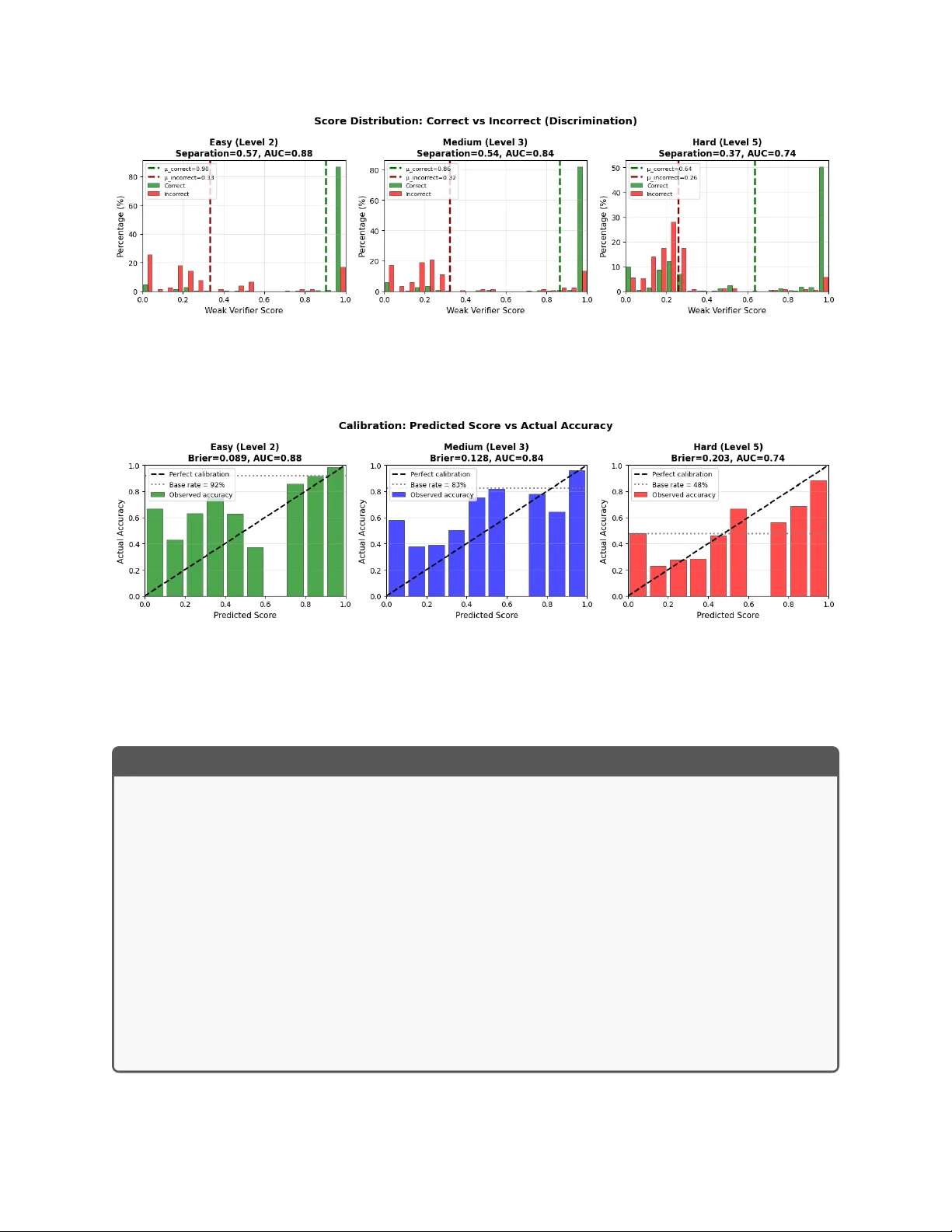
When to Trust the Cheap Check: Weak and Strong Verification for Reasoning

When to T rust the Cheap Chec k: W eak and Strong V erification for Reasoning Sha yan Kiy ani 1 , Sima No orani 1 , George P appas 1 , and Hamed Hassani 1 1 Univ ersity of Pennsylv ania {shayank, nooranis, pappasg, hassani}@seas.upenn.edu F ebruary 20, 2026 Abstract Reasoning with LLMs increasingly unfolds inside a broader v erification lo op. In ternally , systems use c heap chec ks, such as self-consistency or pro xy rew ards, which w e call we ak verific a- tion . Externally , users inspect outputs and steer the mo del through feedback un til results are trust worth y , whic h we call str ong verific ation . These signals differ sharply in cost and reliability: strong v erification can establish trust but is resource-intensiv e, while w eak verification is fast and scalable but noisy and imp erfect. W e formalize this tension through we ak–str ong verific ation p olicies , which decide when to accept or reject based on weak verification and when to defer to strong verification. W e introduce metrics capturing incorrect acceptance, incorrect rejection, and strong-verification frequency . Ov er p opulation, we show that optimal p olicies admit a t wo-threshold structure and that c alibr ation and sharpness gov ern the v alue of weak verifiers. Building on this, we dev elop an online algorithm that pro v ably con trols acceptance and rejection errors without assumptions on the query stream, the language mo del, or the w eak verifier. Exp erimen ts 1 on mathematical reasoning and sequential decision-making demonstrate that our algorithm achiev es reliability comparable to exhaustive strong v erification while significan tly reducing verification cost. 1 In tro duction Recen t adv ances in the reasoning capabilities of large language models hav e b een driv en not only by larger models or increased test-time computation, but critically b y the incorp oration of verification in to the inference pro cess. In practice, verification arises on t wo complemen tary fronts: On the user side, mo del outputs are treated as high-p otential candidates that are sub ject to careful ev aluation. This ev aluation ma y in volv e insp ecting outputs line b y line or, dep ending on the domain, testing them externally in the real world. Crucially , this pro cess is informed b y context, preferences, and domain knowledge that may extend b ey ond what can b e captured textually . While this form of verification enforces the highest level of trust, it is inherently costly; w e refer to it as str ong verific ation . 1 Co de a v ailable at https://github.com/nooranisima/weak- and- strong- verification/tree/main 1 On the model side, verification is engineered to op erate at scale, with the goal of approximating the judgmen ts users mak e under strong v erification. This includes self-consistency , learned critiques, or proxy rewards that attempt to an ticipate what users would agree with. A dditionally , in some domains, sp ecialized tools can pro vide fast, lo cal c hecks of correctness (e.g., b y executing code), but these t ypically certify narrow asp ects of an output rather than whether a line of reasoning is promising ov erall, as an expert would judge. W e refer to this form of fast, scalable verification as we ak verific ation . This con trast highlights a fundamental tension: the mec hanisms that most effectiv ely establish trust are costly to deplo y at scale, while the mec hanisms that scale effortlessly are often insufficient to supp ort reliable use on their own. Therefore, what is missing in current reasoning systems is a principled wa y to orc hestrate v erification sources. W e ask: Can we match the r eliability we would get if str ong verific ation wer e applie d at every step, while deploying it on only a smal l, c ar eful ly chosen fr action of the r e asoning pr o c ess? W e answ er this question affirmatively by developing a principled framework in which internal v erification signals are used not only to refine candidate solutions, but also to inform when stronger v erification should b e called. Our core contribution is a nov el online calibration algorithm, Selective Strong V erification (SSV), that explicitly controls the mismatc h b etw een weak and strong v erification signals on the subset of instances where decisions are made solely based on weak verification, without consulting the strong signal. This enables strong verification resources to b e deploy ed selectiv ely , while preserving reliable end-to-end b eha vior. W e now outline our con tributions and the structure of the pap er. (1) In Section 3 , we formalize we ak–str ong verific ation p olicies : an algorithmic framework that go verns when a system should rely solely on a weak verifier and when it should defer to a strong v erifier. W e introduce three performance metrics that capture the fundamen tal tradeoffs in this setting. The first t wo are typ e-I and typ e-II errors, capturing incorrect trust in the w eak verifier when it disagrees with the strong v erifier: accepting incorrect resp onses or rejecting correct ones. The third metric is the frequency with which the strong verifier is queried. (2) In Section 4 , we characterize optimal w eak–strong verification p olicies under p opulation as- sumptions and sho w that they admit a t wo-threshold structure, whic h underpins our algorithm. Along the wa y , our analysis highligh ts c alibr ation and sharpness as tw o k ey prop erties go verning the effectiv eness of w eak v erifiers, a p ersp ectiv e that ma y b e of indep endent interest. (3) In Section 5 , we develop SSV, a finite-sample, online algorithm that prov ably con trols t yp e-I and t yp e-I I errors. Our guaran tees are fully distribution-free and mak e no assumptions on the query stream, the b ehavior of the language mo del, or the quality of the w eak verifier. (4) In Section 6 , w e ev aluate SSV on outcome-lev el mathematical reasoning and pro cess-lev el sequen tial puzzle solving. W e demonstrate that our algorithm maintains target error rates in finite- samples while enabling principled navigation of the reasoning-verification cost fron tier, ac hieving near-oracle accuracy with significantly few er costly calls. 2 2 Related W orks LLM reasoning and verification. Recent progress in LLM reasoning is driven largely on tw o main axes. First, a large b o dy of work fo cuses on improving the reasoning pro cess via inference-time reasoning, including structured prompting [ 29 , 33 , 34 ], search [ 31 , 32 ], deco ding strategies [ 23 , 30 ], as w ell as training approac hes that elicit longer reasoning c hains [ 22 , 27 ]. These metho ds treat weak signals as fixed and strategize reasoning traces to impro ve final p erformance. Second, complementary work impro ves the w eak v erification signal itself, including LLM-as-judge ev aluation [ 13 ], sp ecialized verifiers [ 19 , 24 ], judge-time scaling [ 11 , 20 ], and pro cess-reward mo dels [ 26 , 28 , 35 ]. Our work is orthogonal to b oth: w e tak e the w eak v erifier and reasoning pro cedure as fixed, and study the lay er ab ov e, orchestrating when to trust the weak signal and when to inv oke costly strong verification. This framew ork applies to an y reasoning pro cedure (single pass, iterative refinemen t, or tree searc h) and any scoring mo del. T o the b est of our knowledge, this in teraction has not b een explicitly form ulated or analyzed. Selectiv e prediction and learning to defer. Algorithmically , our setup relates to selective prediction and learning-to-defer (L2D). Early w ork established theoretical frameworks for classification with a reject option, p osing the problem as risk minimization with explicit rejection costs [ 2 , 6 ]. Rather than fixing confidence thresholds p ost ho c, subsequen t work learns when to abstain as part of training [ 4 , 7 , 8 ], with extensions to the online setting [ 7 ]. The L2D literature extends selectiv e prediction to human-AI collab oration, studying the optimal division of lab or b et ween mo del and exp ert [ 14 – 16 , 25 ]. Our setting can b e viewed as an instance of L2D, where deferral means inv oking strong verification. The combination of distribution-free online calibration, partial feedback, and separate Type-I/I I error control, together with the algorithmic techniques w e dev elop, ma y b e of indep enden t in terest to the broader umbrella of L2D. 3 W eak–Strong V erification P olicies and Metrics W e consider a general v erification-guided reasoning setting inv olving a language mo del and tw o sources of verification. Language mo del and v erification oracles. Let P ∈ P denote a problem instance or prompt that requires reasoning. Let f : P → R denote a language mo del that, given P , generates a (p ossibly random) resp onse R := f ( P ) . W e consider tw o forms of verification. First, let g : P × R → { 0 , 1 } denote a str ong verific ation oracle, whic h outputs a binary judgmen t indicating whether a resp onse is correct. This oracle represents the strongest form of verification av ailable, such as human insp ection or domain sp ecific executions, and serves as the ultimate criterion against which reasoning outcomes are ev aluated. Second, let w : P × R → [0 , 1] denote a we ak verific ation or acle , whic h assigns a real-v alued score to a prompt–resp onse pair, aiming to approximate strong v erification, for example through pro xy rew ards or domain-specific to ols. The contin uous nature of w reflects uncertain t y: it pro vides a confidence signal, with larger v alues indicating greater confidence in correctness. 3 Stream of queries and resp onses. W e assume there exists an arbitrary and unkno wn stream of queries. A t eac h time step t = 1 , 2 , . . . , the language model receives a query P t and pro duces a resp onse R t = f ( P t ) . W e use the notation w t := w ( P t , R t ) and g t := g ( P t , R t ) . W e place no assumptions on how the stream { P t } t ≥ 1 is generated. In particular, queries may b e indep enden t user prompts, in termediate reasoning steps, or any combination thereof, and the stream ma y dep end arbitrarily on past verification outcomes. This mo deling is flexible enough to capture a range of reasoning strategies. F or example, - Eac h P t ma y corresp ond to a user prompt, eac h R t to a full model output. This resembles to a strategy known as output rew ard mo deling in the literature [ 3 ]. - In step-b y-step reasoning, eac h P t ma y consist of a prompt together with the partial solution so far, and eac h R t corresp onds to a single reasoning step. This resembles pro cess reward mo deling in the literature [ 12 ]. In b oth cases, rejecting/accepting resp onses can influence future queries, either by triggering another sample for the same prompt until a budget is exhausted, or by mo ving on to a different prompt. W eak-strong v erification p olicy . A w eak–strong v erification p olicy is a sequence of (p ossibly randomized) functions π t ( · ) : [0 , 1] → { A , R , SV } , ∀ t ≥ 1 , whic h maps a weak verification score to one of three actions: A: accept the resp onse without asking for strong v erification. R: reject the resp onse without asking for strong v erification. SV: query the strong v erifier; accept the resp onse if g ( P , R ) = 1 and reject it otherwise. A t iteration t = 1 , 2 , . . . , the system pro ceeds as follows: - The language mo del generates a resp onse R t = f ( P t ) . - The weak verifier is queried, yielding a score w t . - The p olicy π t ( w t ) determines whether to accept or reject the resp onse, with or without calling strong verification. The p olicy { π t } t> 0 th us gov erns when the weak signal is sufficien t to accept or reject a resp onse, and when the algorithm defers to strong verification g t . Figure 1 depicts the ov erall flo w. P erformance metrics. W e ev aluate a verification p olicy along the interaction sequence, without imp osing any distributional assumptions on the stream { ( P t , R t ) } t ≥ 1 . F or a fixed horizon T ≥ 1 , define the index sets S 0 ( T ) := { t ≤ T : g t = 0 } , S 1 ( T ) := { t ≤ T : g t = 1 } , and their sizes N 0 ( T ) := |S 0 ( T ) | and N 1 ( T ) := |S 1 ( T ) | . W e emphasize that g t alw ays exists conceptually , but is only observed when the strong verifier is queried. W e define the following empirical p erformance quan tities: 4 Figure 1: The arc hitecture of w eak-strong v erification for LLM reasoning. T yp e-I error (incorrect acceptance): 2 Err I ( T ) := 1 N 0 ( T ) T X t =1 1 { g t = 0 , π t ( r t ) = A } . This is the empirical frequency of accepting a resp onse among those rounds where the strong verifier w ould deem it incorrect, i.e., acceptance errors c onditione d on g t = 0 . T yp e-I I error (incorrect rejection): Err II ( T ) := 1 N 1 ( T ) T X t =1 1 { g t = 1 , π t ( r t ) = R } . This is the empirical frequency of rejecting a resp onse among those rounds where the strong v erifier w ould deem it correct, i.e., rejection errors c onditione d on g t = 1 . Strong v erification frequency: SV( T ) := 1 T T X t =1 1 { π t ( r t ) = SV } . This is the a verage rate at whic h the algorithm calls strong verification and th us reflects verification cost or latency . T yp e-I I error and strong v erification frequency impose additional system load, such as increased user latency or higher computational and op erational costs. In con trast, type-I error corresp onds to degraded output qualit y , manifesting as hallucinations or incorrect resp onses, whic h reduces system v alue and ero des trust among downstre am decision mak ers. A go o d verification policy m ust therefore seek to k eep all three quantities small. How ever, there are inherent tradeoffs b etw een them. F or a fixed language mo del, w eak v erifier, and strong verifier, enforcing sufficien tly small t yp e-I and type-I I error rates ma y necessarily require a higher frequency of strong verification calls. This leads to an engineering tradeoff on the service pro vider side: given 2 If N 0 ( T ) = 0 (resp ectiv ely , N 1 ( T ) = 0 ), we set Err I ( T ) = 0 (resp ectiv ely , Err II ( T ) = 0 ). 5 the quality of the language mo del and the av ailable v erification signals, how should one prioritize these comp eting ob jectives? In the next section, w e first take a different route by studying the P areto-optimal tradeoff achiev able b y v erification p olicies ov er p opulation. This allows us to derive the structure of optimal p olicies and to motiv ate sp ecific algorithmic design c hoices. Building up on that, w e then turn to the the goal of con trolling t yp e-I and type-I I errors while minimizing the use of strong verification in the sequen tial setting. 4 F undamen tal T radeoffs of W eak-Strong V erification Here we study the fundamen tal tradeoffs among the three quantities introduced in Section 3 through a simplified, population-level formulation. This is not intended to address the sequen tial problem of Section 3 , but rather to isolate a one-shot v ersion of the problem where tradeoffs can b e c haracterized explicitly . The insights from this p opulation p ersp ectiv e will guide the design of the se quential, distribution-fr e e algorithm developed in the next section. P opulation-lev el form ulation. W e consider a one-shot setting in whic h a prompt–resp onse pair ( P , R ) is drawn from a join t distribution D , with R = f ( P ) . The language mo del f , weak verifier w : P × R → [0 , 1] , and strong v erifier g : P × R → { 0 , 1 } are treated as fixed. A weak–strong verification p olicy is a mapping π : [0 , 1] → { A , R , SV } , whic h assigns an action based on the weak score w ( P , R ) . Time indices are unnecessary in this one-shot setting. P opulation metrics. W e define probabilistic coun terparts of the empirical quantities from Sec- tion 2: • T yp e-I error: Pr D [ π ( w ( P , R )) = A | g ( P , R ) = 0] . • T yp e-I I error: Pr D [ π ( w ( P , R )) = R | g ( P , R ) = 1] . • Strong v erification rate: Pr D [ π ( w ( P , R )) = SV] . These metrics abstract aw ay temp oral dep endence and allo w us to study intrinsic tradeoffs in exp ectation. P areto-optimal tradeoffs. F or λ 1 , λ 2 ≥ 0 , we study π ⋆ ( λ 1 ,λ 2 ) ∈ arg min π Pr[ π ( w ( P , R )) = SV] (1) + λ 1 Pr[ π ( w ( P , R )) = A | g ( P , R ) = 0] + λ 2 Pr[ π ( w ( P , R )) = R | g ( P , R ) = 1] . Sw eeping ( λ 1 , λ 2 ) v aries the relativ e p enalty assigned to t yp e-I errors, type-I I errors, and strong- v erification calls, thereby encoding differen t operating points (e.g., prioritize reliabilit y vs. la- tency/cost). The resulting optimizers π ⋆ ( λ 1 ,λ 2 ) trace the set of P areto-optimal p olicies, revealing whic h p erformance lev els are ac hiev able. 6 Assumption 4.1 (Calibration of the w eak verifier) . The weak v erification oracle r is calibrated with resp ect to the strong verifier g in the following sense: for all p ∈ [0 , 1] , Pr  g ( P , R ) = 1   w ( P , R ) = p  = p, where ( P , R ) is distributed as P ∼ D and R = f ( P ) . Assumption 4.1 is a natural starting p oint: without some link b etw een the w eak score w ( P , R ) and the correctness signal g ( P , R ) , the weak v erifier could in principle b e arbitrary and carry no actionable information. While we do not rely on calibration in the next section, it provides a clean p opulation mo del in whic h we can derive structural insights ab out how weak and strong verification should interact. Theorem 4.2 (Structure of an optimal p olicy) . Supp ose Assumption 4.1 holds. F or any λ 1 , λ 2 ≥ 0 , ther e exists an optimal p olicy π ⋆ ( λ 1 , λ 2 ) that has a thr eshold structur e: ther e exist thr esholds t low , t high ∈ [0 , 1] such that π ⋆ ( w ) ∈      { R } , w < t low , { SV } , t low ≤ w ≤ t high , { A } , w > t high . Theorem 4.2 aligns with the follo wing intuition: when the weak v erifier is sufficien tly confiden t that a resp onse is incorrect (small w ), it is optimal to reject; when it is sufficiently confiden t that a resp onse is correct (large w ), it is optimal to accept; and when the w eak signal is am biguous (intermediate w ), it is optimal to defer to strong verification. In particular, calibration makes the w eak score directly in terpretable as a probabilit y of correctness, which in turn mak es it easy to translate into A/R/SV decisions. Ho wev er, calibration is not the only relev an t prop ert y of a w eak verifier. Ev en a calibrated weak v erifier can b e unhelpful if it is uninformative . F or example, a v erifier that alw ays outputs the marginal probabilit y Pr [ g ( P , R ) = 1] is p erfectly calibrated, y et carries no instance-sp ecific information and is therefore uninformative. What prop erties of the weak v erifier matter? The next proposition characterizes the v alue of the optimal ob jective and makes precise how the distribution of weak scores go verns the ac hiev able tradeoff. Prop osition 4.3 (V alue of the optimal ob jective) . Assume Assumption 4.1 . L et W := w ( P , R ) ∈ [0 , 1] , α 0 := Pr [ g ( P , R ) = 0] and α 1 := Pr [ g ( P , R ) = 1] . Then the minimum value of the obje ctive in ( 1 ) c an b e written as V ( λ 1 , λ 2 ) = E  min n 1 , λ 1 α 0 (1 − W ) , λ 2 α 1 W o  . Interpr etation. The three terms inside the min corresp ond to the three actions at a given weak score W : (i) calling strong verification costs 1 ; (ii) accepting without strong verification risks a type-I mistake, which under calibration o ccurs with probabilit y 1 − W and is weigh ted by λ 1 (after normalizing by ho w often g = 0 o ccurs, via α 0 ); (iii) rejecting without strong v erification risks a type-I I mistake, which under calibration o ccurs with probabilit y W and is weig hted by λ 2 (normalized by α 1 ). Thus the optimal policy , p oin twise in W , chooses the cheapest of these three options, and the optimal v alue is the exp ected cost of that choice. 7 This expression makes clear that, b eyond calibration, the sharpness of the w eak verifier plays a crucial role. Here, sharpness refers to how often W tak es v alues near 0 or 1 , i.e., confidently accepts or rejects. If W is often close to 0 , then rejection is cheap b ecause the type-I I risk W is small; if W is often close to 1 , then acceptance is cheap b ecause the t yp e-I risk 1 − W is small. In b oth cases, the p olicy can av oid strong v erification while k eeping errors small. In contrast, if W is typically am biguous (e.g., concentrated near 1 / 2 ), then b oth risks W and 1 − W are non-negligible, so the minim um is t ypically close to 1 , forcing the policy to rely more frequently on strong v erification. T ak eaw ay . T w o complementary prop erties gov ern the usefulness of a weak verifier: c ali- br ation mak es its scores in terpretable as correctness probabilities, while sharpness makes it effectiv e by pro ducing decisive scores near 0 or 1 . This message may b e useful for practitioners designing and ev aluating scalable w eak v erifiers, although w e do not revisit it further in this pap er. In con trast, the threshold structure of Theorem 4.2 will serv e as a key structural cornerstone for the algorithm developed in the next section. 5 Selectiv e Strong V erification and Guaran tees In this section, we design Selectiv e Strong V erification (SSV), an algorithm for the sequential problem in tro duced in Section 3 , fixing a language mo del f , a w eak verifier w , and a strong verifier g . Building on the t wo-thresho ld structure identified in Section 4 , w e construct a p olicy that adaptively decides, based on the weak score w t , whether to accept, reject, or query strong v erification. W e make no assumptions on the query stream, the verification signals, or the b eha vior of the language mo del. Our goal is to control the empirical type-I and type-I I errors Err I ( T ) and Err II ( T ) , defined as in Section 3 , b y enforcing these constraints uniformly over time , in the sense that for every T and user-defined α and β , Err I ( T ) ≤ α and Err II ( T ) ≤ β . This goal is ac hieved by the end of this section: Theorem 5.1 establishes that the prop osed algorithm enjo ys distribution-free, uniform-in-time control of type-I and type-I I errors up to finite-sample slac k terms. Algorithm design. Algorithm 1 induces a p olicy via tw o adaptiv e thresholds ( τ t R , τ t A ) and ex- ploration probabilities ( q t A , q t R ) . Looking at the Thr e e r e gions step of Algorithm 1 , at time t , the w eak score w t places the resp onse into one of three regions: an ac c ept r e gion ( w t > τ t A ), a r eje ct r e gion ( w t < τ t R ), or an unc ertain r e gion (b etw een the thresholds). In the uncertain region, the p olicy alwa ys queries the strong verifier. In the accept and reject regions, the resp onse is accepted or rejected, without observing the strong signal g t , with high probabilit y (think of ( q t A , q t R ) as small). With a small probability , the p olicy instead queries the strong verifier and follo ws its outcome. W e explain the necessity of this randomized exploration later. Threshold up dates. As is clear from the Thr eshold up date step of Algorithm 1 , the thresholds are up dated only at rounds where the strong signal g t is observed. Consider the up date of the accept threshold, τ t +1 A ← max ( τ t R , τ t A + η t 1 { g t = 0 }  1 { w t > τ t A } − α  q t ) . 8 Algorithm 1 Selective Strong V erification (SSV) Require: T argets α, β ∈ (0 , 1) ; exploration probabilities { q t A , q t R } t ≥ 1 ; step sizes { η t } t ≥ 1 ; initial thresholds τ 1 R ≤ τ 1 A for t = 1 , 2 , . . . do Receiv e query and resp onse ( P t , R t ) w t ← w ( P t , R t ) {weak verification score} Thr e e r e gions if w t > τ t A then a t ← A w.p. 1 − q t A , else a t ← SV. Also, set q t = q t A . else if w t < τ t R then a t ← R w.p. 1 − q t R , else a t ← SV. Also, set q t = q t R . else a t ← SV. Also, set q t = 1 . end if Final de cision and fe e db ack if a t = A then accept R t ; contin ue else if a t = R then reject R t ; contin ue else Observ e g t ← g ( P t , R t ) {strong verification} if g t = 1 then accept R t else reject R t end if Thr eshold up dates τ t +1 A ← max  τ t R , τ t A + η t 1 { g t =0 }  1 { w t >τ t A }− α  q t  τ t +1 R ← min  τ t +1 A , τ t R + η t 1 { g t =1 }  β − 1 { w t <τ t R }  q t  end if if a t  = SV then τ t +1 R ← τ t R , τ t +1 A ← τ t A end if end for The outer max {·} acts as a pro jection step that enforces the ordering constraint τ t R ≤ τ t A at all times and prev ents the thresholds from crossing. The second term inside the maximum is resp onsible for error tracking: since τ t A con trols incorrect acceptances, the up date is active only when g t = 0 , corresp onding to a p oten tial type-I error. The term 1 { w t > τ t A } − α driv es the empirical rate of accepting among such rounds to ward the target lev el α . Finally , the division by q t corrects for the fact that strong feedbac k is observ ed at random times with probabilities that dep end on the weak signal, yielding an unbiased update via standard imp ortance weigh ting. The update for τ t +1 R is defined analogously to control t yp e-I I error. Wh y randomized strong verification is necessary . The error quan tities ab o ve are defined c onditional ly on the str ong verifier . F or example, the type-I error measures the rate of acceptances among times when g t = 0 . If the p olicy deterministically accepts or rejects without querying the strong verifier, then g t remains unobserved, and the algorithm receives no direct feedback ab out whether that decision con tributed to t yp e-I or t yp e-I I error. This w ay , the interaction ma y enter a regime where (for instance) w t > τ t A almost alw ays, leading to many acceptances but essen tially no strong-v erification feedback. In such regimes, violations of the error constraints cannot b e detected 9 or corrected without additional assumptions. Algorithm 1 av oids this issue b y querying the strong v erifier with small probabilities q t A and q t R ev en in decisiv e regions. The following theorem shows that Algorithm 1 controls the empirical errors for any T (up to finite-sample slack terms), without an y assumptions on the stream { ( P t , R t ) } t ≥ 1 . Theorem 5.1 (Finite-time empirical error control) . Fix a horizon T ≥ 1 . Run Algorithm 1 with a c onstant step size η t = η > 0 ( ∀ , t ) and pr e dictable str ong-query pr ob abilities { q t } T t =1 satisfying q t ∈ (0 , 1] and q min := min t ≤ T  q t A , q t R  > 0 . Assume the initial thr esholds satisfy τ 1 R ≤ τ 1 A with τ 1 R , τ 1 A ∈ [0 , 1] . Then for any δ ∈ (0 , 1) , with pr ob ability at le ast 1 − δ over the algorithm’s internal r andomness, Err I ( T ) ≤ α + ∆  N 0 ( T ) , δ  , Err II ( T ) ≤ β + ∆  N 1 ( T ) , δ  , wher e ∆( N , δ ) := 1 + 2 η q min η N + s 2 log(4 /δ ) N q min + log(4 /δ ) 3 N q min , with the c onvention ∆(0 , δ ) = 0 . The error b ound decomp oses into tw o qualitatively differen t sources. The first term, of order 1 / ( η N ) , reflects the intrinsic error of trackin g a target quan tile with an online threshold up date: ev en in an idealized setting where the strong signal were alw ays revealed after eac h decision, this term would remain. It is the same fundamental limitation that app ears in online conformal prediction and other quan tile-trac king pro cedures [ 1 , 9 , 18 ]. The remaining tw o terms arise from partial access to the strong signal and the randomized exploration required to obtain unbiased feedback. Their dep endence on q min is insightful: larger exploration probabilities make error control easier, but increase the frequency of strong v erification calls. This highlights an inherent algorithmic trade-off induced by our design—balancing statistical accuracy against v erification cost—and suggests that, in practice, the exploration probabilities should b e treated as tunable hyperparameters to ac hieve the b est p erformance. 6 Exp erimen tal Results In this section, we empirically ev aluate SSV (Algorithm 1 ) across tw o distinct reasoning paradigms, demonstrating the generality of the problem formulation in Section 3 . The first scenario considers outcome-level v erification, consisten t with the Outcome Rew ard Mo deling (ORM) paradigm [ 3 ]. Here, the system ev aluates a complete candidate solution after it has b een fully generated. W e utilize the MA TH dataset [ 10 ], a rigorous benchmark for mathematical problem- solving. F ollo wing the notation in Section 3 , a query P t represen ts a user prompt, and R t is a complete resp onse candidate. The mo del generates resp onses sequentially; the policy π t ev aluates eac h via its weak score w t un til a candidate is accepted or the budget n is exhausted. T o test SSV across v arying complexities, w e conduct exp eriments on problems from difficulty levels 2, 3, and 5. The second scenario fo cuses on step-by-step verification, mirroring Pro cess Reward Mo deling (PRM) [ 12 ]. W e ev aluate this using Sudoku puzzles [ 21 ], where the fo cus shifts to granular, sequential 10 (a) MA TH: Type-I Error (Ac- cept) (b) MA TH: T yp e-II Error (Reject) (c) Sudoku: Combined Er- rors Figure 2: Empirical Error Rate Con vergence. Running-av erage error rates 1 T P T t =1 err t for target lev els α = β = 0 . 15 . Left and Cen ter (MA TH): Con vergence of T yp e-I and T yp e-I I errors across three difficulty levels in the outcome level verification task. Right (Sudoku): Conv ergence in the sequential step-by-step reasoning task. decision-making. In this task, P t represen ts the curren t b oard state (initial puzzle plus all accepted digits), and R t is the mo del’s prop osed next digit and its co ordinates. Sudoku is a high-stakes en vironment where a single incorrect step often renders the entire puzzle unsolv able, testing the p olicy’s abilit y to in tercept errors at the step level while minimizing calls to the costly strong v erifier. W e provide sp ecific implementation details for the weak and strong verifiers used in each task in App endix B.4 . Our goal is to show that across b oth tasks, SSV (Algorithm 1 ) successfully controls empirical Type-I and T yp e-I I errors at their nominal levels. F urthermore, w e show that our approac h allows a service pro vider to principledly in terp olate b etw een tw o op erational extremes. On one end is the W e ak-Only r e gime , where the system relies solely on the weak verifier. This represen ts the absolute lo wer b ound for computation ov erhead and latency caused b y using a strong verification as it bypasses strong v erifier entirely; ho wev er this efficiency comes at the cost of reasoning accuracy and user trust. On the opp osite end is the Str ong-Only r e gime , where ev ery query is routed to the strong verifier. while this maximizes reasoning p erformance and reliabilit y , it incurs the highest p ossible op erational costs and latency . W e demonstrate that SSV can identify a fav orable balance, maintaining high reasoning p erformance while significantly reducing the load on the strong verifier. Exp erimen tal Setup and Metrics. W e report results along tw o primary axes. First, w e measure empirical Type-I and T yp e-I I error rates (Section 3 ) to v alidate that our algorithm controls these quantities under non-stationary conditions. Second, w e assess the reasoning p erformance vs. v erification-cost (measured by the strong-verification frequency SV ( T ) ) trade-off b y sw eeping the target error levels ( α, β ) . Baselines. W e compare our p olicy against tw o baselines that represent the theoretical and practical b oundaries of the system. The Strong-Only (Oracle) baseline in vok es the strong v erifier for ev ery query , representing the maxim um achiev able reasoning accuracy and the upp er b ound for op erational cost. Conv ersely , the W eak-Only (Greedy) baseline represents the minimum-cost regime; here, the system generates n candidates and selects the one with the highest weak verification score to b e accepted as the final result or the next reasoning step, bypassing the strong v erifier en tirely . 11 6.1 Empirical Error Con trol W e first ev aluate the abilit y of SSV (Algorithm 1 ) to maintain target error lev els. Figure 2 displays the running aver age of the Type-I and Type-I I error rates as the in teraction sequence progresses, defined at time step T as 1 T P T t =1 err t . Here, the index t iterates ov er the global stream of verification decisions across all problems in each dataset. A cross b oth the mathematical reasoning tasks (Fig. 2 a, b) and the sequential Sudoku steps (Fig. 2 c), the running a verage errors stabilize near the nominal targets of α = β = 0 . 15 . This confirms the result of Theorem 5.1 . The tra jectories reflect the t ypical b ehavior of online quantile trac king, where the learning rate η go verns the trade-off b etw een adaptation sp eed and stabilit y . 3 (a) MA TH (Level 2) (b) MA TH (Level 3) (c) MA TH (Level 5) (d) Sudoku Figure 3: Reasoning A ccuracy vs. V erification Cost T radeoffs. SSV (Algorithm 1 ) (A daptive: solid colored lines) interpolates b et ween the Strong-Only Oracle (black star) and the W eak-Only baselines (colored circles). Left (MA TH): T radeoff curves for Easy , Medium, and Hard problems; Righ t (Sudoku): T radeoff curv e for Sudoku step-by-step reasoning task. p oints are lab eled with nominal error targets where α = β . 6.2 Reasoning Performance vs. V erification Cost T o c haracterize our framework’s op erational p otential, we sw eep the error targets ( α, β ) and plot reasoning accuracy against the av erage num b er of strong-verifier calls p er problem. This visualization rev eals the P areto fron tier of the accuracy-v erification-cost trade-off, spanning the zero-cost W eak- Only baseline to the high-reliabilit y Strong-Only Oracle. SSV serves as a principled mechanism to na vigate and realize this fron tier, allowing service providers to interpolate b et ween these regimes by desired reliability b ounds. The intrinsic efficiency of the Pareto curve (as reflected b y its slop e, that is, ho w m uch accuracy is gained p er unit of strong v erification cost) is fundamentally go verned b y the w eak v erifier signals. The algorithm’s role is then to leverage this sharpness b y dynamically iden tifying whic h reasoning steps require strong verification. In the Easy MA TH subsets and the Sudoku task, the w eak signals exhibit high sharpness, resulting in steep er curves. In these cases, the inheren t quality of the signals enables near-Oracle accuracy with only a fraction of the strong verifier calls. F or instance, in Sudoku, the Strong-Only Oracle reaches an accuracy of 44.2% with 5.32 strong calls p er puzzle. In contrast, 3 Larger v alues of η facilitate faster initial conv ergence but result in noisier tra jectories, while smaller v alues produce smo other curves with slow er conv ergence. 12 our adaptive p olicy achiev es a comparable 43.1% accuracy (at α = β = 0 . 01 ) while requiring only 2.87 strong calls—a 46% reduction in the load on the strong verifier. In the hardest MA TH setting (lev el 5), the relationship is more linear: as the w eak signals b ecome less decisiv e, higher accuracy requires an appro ximately prop ortional increase in strong verification. Y et SSV still concen trates resources where they are most needed, reac hing 60% accuracy with 2 calls p er problem, compared to the Oracle’s 2.8 calls for 63.5% accuracy . F or a detailed analysis of the w eak verification scores, refer to App endix B.3 . Finally , w e observe a compounded verification efficiency in the sequen tial reasoning setting. As sho wn in the last column of T able 1 , SSV is more query-efficient with the w eak verifier than the W eak-Only baseline. While the W eak-Only baseline requires 6.00 weak calls p er puzzle to reach its lo wer success rate, our p olicy a verages b etw een 4.8–5.2 weak calls across all op erating p oin ts. This suggests that b y explicitly mo deling uncertain ty through adaptiv e thresholds, SSV a voids redundant reasoning steps. It achiev es this in t wo wa ys: by accepting a confiden t result early or b y escalating immediately to the strong verifier when the weak signal is deemed insufficient to supp ort the target reliabilit y . This immediate escalation b ypasses further weak verification cycles that are statistically lik ely to b e uninformative. T able 1: P erformance T radeoffs on Sudoku. Detailed comparison across different error regimes. Method Accuracy Strong/Puzzle W eak/Puzzle Strong Baseline (Oracle) 44.2% 5.32 – SSV ( α = β = 0 . 001 ) 43.1% 3.31 5.22 SSV ( α = β = 0 . 01 ) 43.1% 2.87 5.19 SSV ( α = β = 0 . 03 ) 42.7% 2.14 5.20 SSV ( α = β = 0 . 05 ) 42.1% 2.06 5.22 SSV ( α = β = 0 . 10 ) 39.0% 1.24 5.18 SSV ( α = β = 0 . 20 ) 36.2% 0.76 5.04 SSV ( α = β = 0 . 30 ) 34.5% 0.68 4.84 W eak Baseline (Greedy) 33.6% 0.00 6.00 Summary of Results. A cross b oth mathemat- ical reasoning and sequen tial puzzle-solving, our exp erimen ts yield three k ey findings. First, SSV consisten tly maintains target error rates with- out prior kno wledge of the query distribution or v erifier quality . Second, our framework provides a smo oth Pareto frontier that allo ws users to prioritize either reasoning quality or op erational cost. Finally , by identifying and acting up on the "sharpness" of the w eak signal, SSV achiev es near-oracle p erformance with a fraction of the exp ensiv e v erification load when possible. 7 Discussion and F uture W ork W e in tro duced a principled algorithmic framework for orchestrating weak and strong verification in LLM reasoning, showing–both theoretically and empirically–that it is p ossible to achiev e reasoning p erformance comparable to alwa ys applying strong verification while querying the strong verifier only a small fraction of the time. A key limitation of the current framework is that the decision to use strong verification dep ends only on the weak score, and not on the broader prompt–resp onse con text ( P t , R t ) ; consequently , our guarantees con trol type-I and type-I I errors only in a marginal sense, av eraged o ver all rounds. W e view this as a mo deling choice rather than a fundamental limitation. Incorp orating contextual dep endence in to weak–strong v erification p olicies could enable finer-grained and more efficien t allo cation of strong verification, but requires more complex online calibration procedures, including context-dependent thresholds and conditional error con trol under partial feedback. W e leav e this as an imp ortan t direction for future work. 13 Impact Statement This work provides a principled framework for allo cating costly verification resources in reasoning systems, enabling reliable use of large language mo dels at scale. By reducing unnecessary human and computational v erification while preserving correctness guarantees, our approach can lo wer deplo yment costs and improv e the safet y and trustw orthiness of AI-assisted decision making across high-stak es domains. References [1] Angelop oulos, A. N., Candes, E. J., and Tibshirani, R. J. Conformal pid control for time series prediction, 2023. URL . [2] Bartlett, P . L. and W egk amp, M. H. Classification with a reject option using a hinge loss. J. Mach. L e arn. R es. , 9:1823–1840, June 2008. ISSN 1532-4435. [3] Cobb e, K., K osara ju, V., Bav arian, M., Chen, M., Jun, H., Kaiser, L., Plapp ert, M., T worek, J., Hilton, J., Nak ano, R., Hesse, C., and Sc hulman, J. T raining verifiers to solv e math word problems, 2021. URL . [4] Cortes, C., DeSalvo, G., and Mohri, M. Theory and algorithms for learning with rejection in binary classification. A nnals of Mathematics and Artificial Intel ligenc e , pp. 1–39, 2023. URL https://api.semanticscholar.org/CorpusID:266252172 . [5] DeepSeek-AI. Deepseek-v3 technical rep ort, 2024. [6] El-Y aniv, R. and Wiener, Y. On the foundations of noise-free selective classification. Journal of Machine L e arning R ese ar ch , 11(53):1605–1641, 2010. URL http://jmlr.org/papers/v11/ el- yaniv10a.html . [7] Gangrade, A., Kag, A., Cutkosky , A., and Saligrama, V. Online selective classification with limited feedback, 2021. URL . [8] Geifman, Y. and El-Y aniv, R. Selectiv e classification for deep neural net works, 2017. URL https://arxiv.org/abs/1705.08500 . [9] Gibbs, I. and Candès, E. A daptive conformal inference under distribution shift, 2021. URL https://arxiv.org/abs/2106.00170 . [10] Hendryc ks, D., Burns, C., Kada v ath, S., Arora, A., Basart, S., T ang, E., Song, D., and Steinhardt, J. Measuring mathematical problem solving with the math dataset, 2021. URL https://arxiv.org/abs/2103.03874 . [11] Kalra, N. and T ang, L. V erdict: A library for scaling judge-time compute, 2025. URL https://arxiv.org/abs/2502.18018 . [12] Ligh tman, H., K osara ju, V., Burda, Y., Edw ards, H., Baker, B., Lee, T., Leike, J., Sc hulman, J., Sutskev er, I., and Cobbe, K. Let’s verify step by step, 2023. URL 2305.20050 . 14 [13] Liu, Y., Iter, D., Xu, Y., W ang, S., Xu, R., and Zhu, C. G-ev al: Nlg ev aluation using gpt-4 with b etter human alignment, 2023. URL . [14] Mozannar, H. and Sontag, D. Consisten t estimators for learning to defer to an exp ert, 2021. URL . [15] Mozannar, H., Lang, H., W ei, D., Sattigeri, P ., Das, S., and Son tag, D. Who should predict? exact algorithms for learning to defer to humans, 2023. URL . [16] Ok ati, N., De, A., and Gomez-Rodriguez, M. Differentiable learning under triage, 2021. URL https://arxiv.org/abs/2103.08902 . [17] Op enAI. Gpt-4o system card, 2024. URL https://openai.com/index/gpt- 4o- system- card/ . [18] Ramalingam, R., Kiy ani, S., and Roth, A. The relationship b etw een no-regret learning and online conformal prediction. arXiv pr eprint arXiv:2502.10947 , 2025. [19] Saad-F alcon, J., Khattab, O., P otts, C., and Zaharia, M. Ares: An automated ev aluation framew ork for retriev al-augmented generation systems, 2024. URL 2311.09476 . [20] Saad-F alcon, J., Lafuen te, A. G., Natara jan, S., Maru, N., T o dorov, H., Guha, E., Buchanan, E. K., Chen, M., Guha, N., Ré, C., and Mirhoseini, A. Archon: An arc hitecture search framework for inference-time techniques, 2025. URL . [21] Shahab, A. mini-sudoku dataset. https://huggingface.co/datasets/asadshahab/ mini- sudoku , 2023. Accessed: 2026-01-27. [22] Shao, Z., W ang, P ., Zhu, Q., Xu, R., Song, J., Bi, X., Zhang, H., Zhang, M., Li, Y. K., W u, Y., and Guo, D. Deepseekmath: Pushing the limits of mathematical reasoning in op en language mo dels, 2024. URL . [23] Sun, H., Haider, M., Zhang, R., Y ang, H., Qiu, J., Yin, M., W ang, M., Bartlett, P ., and Zanette, A. F ast b est-of-n deco ding via sp eculative rejection, 2024. URL 20290 . [24] T ang, L., Laban, P ., and Durrett, G. Minic heck: Efficient fact-chec king of llms on grounding do cumen ts, 2024. URL . [25] V erma, R. and Nalisnic k, E. Calibrated learning to defer with one-vs-all classifiers, 2022. URL https://arxiv.org/abs/2202.03673 . [26] W ang, P ., Li, L., Shao, Z., Xu, R. X., Dai, D., Li, Y., Chen, D., W u, Y., and Sui, Z. Math- shepherd: V erify and reinforce llms step-b y-step without h uman annotations, 2024. URL https://arxiv.org/abs/2312.08935 . [27] W ang, Y., Y ang, Q., Zeng, Z., Ren, L., Liu, L., P eng, B., Cheng, H., He, X., W ang, K., Gao, J., Chen, W., W ang, S., Du, S. S., and Shen, Y. Reinforcement learning for reasoning in large language mo dels with one training example, 2025. URL . [28] W ang, Z., Dong, Y., Zeng, J., Adams, V., Sreedhar, M. N., Egert, D., Delalleau, O., Scow croft, J. P ., Kant, N., Sw op e, A., and Kuchaiev, O. Helpsteer: Multi-attribute helpfulness dataset for steerlm, 2023. URL . 15 [29] W ei, J., W ang, X., Sch uurmans, D., Bosma, M., Ic hter, B., Xia, F., Chi, E., Le, Q., and Zhou, D. Chain-of-though t prompting elicits reasoning in large language mo dels, 2023. URL https://arxiv.org/abs/2201.11903 . [30] Xia, H., Ge, T., W ang, P ., Chen, S.-Q., W ei, F., and Sui, Z. Sp eculativ e deco ding: Exploiting sp eculativ e execution for accelerating seq2seq generation, 2023. URL 2203.16487 . [31] Xie, Y., Kaw aguc hi, K., Zhao, Y., Zhao, X., Kan, M.-Y., He, J., and Xie, Q. Self-ev aluation guided b eam search for reasoning, 2023. URL . [32] Xie, Y., Goy al, A., Zheng, W., Kan, M.-Y., Lillicrap, T. P ., Kaw aguc hi, K., and Shieh, M. Mon te carlo tree search b o osts reasoning via iterative preference learning, 2024. URL https://arxiv.org/abs/2405.00451 . [33] Y ao, S., Y u, D., Zhao, J., Shafran, I., Griffiths, T. L., Cao, Y., and Narasimhan, K. T ree of thoughts: Deliberate problem solving with large language mo dels, 2023. URL https: //arxiv.org/abs/2305.10601 . [34] Y ao, S., Zhao, J., Y u, D., Du, N., Shafran, I., Narasimhan, K., and Cao, Y. React: Synergizing reasoning and acting in language mo dels, 2023. URL . [35] Zhang, L., Hosseini, A., Bansal, H., Kazemi, M., Kumar, A., and Agarwal, R. Generativ e v erifiers: Rew ard mo deling as next-token prediction, 2025. URL . 16 App endix T able of Con ten ts A Pro ofs 18 B Additional Exp erimen ts 24 B.1 Additional Error Con trol Results . . . . . . . . . . . . . . . . . . . . . . . . . . . . . 24 B.1.1 Outcome-Lev el V erification (MA TH Dataset) . . . . . . . . . . . . . . . . . . 24 B.1.2 Step-b y-step V erification (Sudoku) . . . . . . . . . . . . . . . . . . . . . . . . 24 B.2 Detailed Reasoning-Cost T radeoffs . . . . . . . . . . . . . . . . . . . . . . . . . . . . 26 B.3 Analysis of W eak V erifier Scores . . . . . . . . . . . . . . . . . . . . . . . . . . . . . . 27 B.4 V erifier Implementation Details and Prompt Specifications . . . . . . . . . . . . . . . 29 17 A Pro ofs Pro of of Theorem 4.2 and Prop osition 4.3 : Pr o of. Let ( P , R ) be distributed as P ∼ D and R = f ( P ) . Define the random v ariables W := w ( P , R ) ∈ [0 , 1] , g := g ( P , R ) ∈ { 0 , 1 } , and let α 0 := Pr [ g = 0] and α 1 := Pr [ g = 1] . Assume α 0 , α 1 > 0 (otherwise the conditional error terms in (1) are v acuous and the problem is trivial). F or λ 1 , λ 2 ≥ 0 , consider the p opulation ob jective V ( λ 1 , λ 2 ) := min π :[0 , 1] →{ A,R,S V } Pr[ π ( W ) = S V ] + λ 1 Pr[ π ( W ) = A | g = 0] + λ 2 Pr[ π ( W ) = R | g = 1] . Define the effective weigh ts a := λ 1 α 0 , b := λ 2 α 1 . Claim A.1 (Unconditional and p oin twise form) . Under Assumption 3.1 (c alibr ation), the obje ctive c an b e written as V ( λ 1 , λ 2 ) = min π :[0 , 1] →{ A,R,S V } E  ℓ  W , π ( W )  , wher e the p ointwise action c osts ar e ℓ ( w , S V ) = 1 , ℓ ( w , A ) = a (1 − w ) , ℓ ( w, R ) = bw . Mor e over, an optimal p olicy c an b e chosen deterministic al ly and p ointwise: π ⋆ ( w ) ∈ arg min u ∈{ A,R,S V } ℓ ( w , u ) for al l w ∈ [0 , 1] , and henc e V ( λ 1 , λ 2 ) = E [min { 1 , a (1 − W ) , bW } ] . Pr o of. First rewrite the conditional terms: Pr[ π ( W ) = A | g = 0] = Pr[ π ( W ) = A, g = 0] α 0 , Pr[ π ( W ) = R | g = 1] = Pr[ π ( W ) = R, g = 1] α 1 . Th us, V ( λ 1 , λ 2 ) = min π  Pr[ π ( W ) = S V ] + a Pr[ π ( W ) = A, g = 0] + b Pr[ π ( W ) = R, g = 1]  . Conditioning on W and using the law of total exp ectation, Pr[ π ( W ) = A, g = 0] = E [ 1 { π ( W ) = A } Pr( g = 0 | W )] , Pr[ π ( W ) = R, g = 1] = E [ 1 { π ( W ) = R } Pr( g = 1 | W )] . By Assumption 3.1, Pr( g = 1 | W ) = W and Pr( g = 0 | W ) = 1 − W , so V ( λ 1 , λ 2 ) = min π E [ 1 { π ( W ) = S V } + a 1 { π ( W ) = A } (1 − W ) + b 1 { π ( W ) = R } W ] = min π E  ℓ  W , π ( W )  , 18 with ℓ as stated. F or the p oin twise optimalit y: for each w , the quan tity inside the exp ectation dep ends on π only through the c hosen action at w . If π is randomized, then conditional on W = w its exp ected cost is a con vex combination of { ℓ ( w , A ) , ℓ ( w , R ) , ℓ ( w , S V ) } , whic h is minimized b y placing all mass on an action that attains the minim um. Th us an optimal p olicy exists that is deterministic and satisfies π ⋆ ( w ) ∈ arg min u ℓ ( w , u ) for all w , and the optimal v alue is V ( λ 1 , λ 2 ) = E [min { 1 , a (1 − W ) , bW } ] . The v alue iden tity in the claim is exactly Prop osition 3.3. It remains to sho w the threshold structure of an optimal p olicy (Theorem 3.2) by comparing the three affine costs. If a = 0 , then ℓ ( w , A ) ≡ 0 is p oin twise minimal and π ⋆ ( w ) ≡ A . If b = 0 , then ℓ ( w , R ) ≡ 0 is p oint wise minimal and π ⋆ ( w ) ≡ R . Assume henceforth a > 0 and b > 0 , and define t low := 1 b , t high := 1 − 1 a . Observ e that ℓ ( w , S V ) ≤ ℓ ( w , R ) iff 1 ≤ bw iff w ≥ t low , and ℓ ( w , S V ) ≤ ℓ ( w , A ) iff 1 ≤ a (1 − w ) iff w ≤ t high . Therefore, whenever t low ≤ t high , we hav e for every w ∈ [ t low , t high ] that ℓ ( w , S V ) = 1 ≤ bw = ℓ ( w , R ) and ℓ ( w , S V ) = 1 ≤ a (1 − w ) = ℓ ( w , A ) , so S V is p oin twise optimal on [ t low , t high ] . F or w < t low , w e ha ve bw < 1 , and also w < t low ≤ t high implies w < 1 − 1 a , i.e. a (1 − w ) > 1 . Hence ℓ ( w , R ) = bw < 1 = ℓ ( w , S V ) < a (1 − w ) = ℓ ( w , A ) , so R is p oin twise optimal. Similarly , for w > t high , we hav e a (1 − w ) < 1 , and w > t high ≥ t low implies bw > 1 , so ℓ ( w , A ) < ℓ ( w , S V ) ≤ ℓ ( w , R ) and A is p oint wise optimal. Th us, when t low ≤ t high , one optimal p olicy is π ⋆ ( w ) =      R, w < t low , S V , t low ≤ w ≤ t high , A, w > t high , with arbitrary tie-breaking at the thresholds, establishing the t wo-threshold structure in Theorem 3.2. Finally , in the three-region regime t low ≤ t high , the v alue formula can b e expanded by splitting the ev ent { W < t low } , { t low ≤ W ≤ t high } , and { W > t high } : V ( λ 1 , λ 2 ) = b E [ W 1 { W < t low } ] + Pr( t low ≤ W ≤ t high ) + a E [(1 − W ) 1 { W > t high } ] . This completes the pro of of b oth results. Pro of of Theorem 5.1 : Pr o of. W e pro ve the type-I and t yp e-I I b ounds simultaneously via a common template. The key idea is that the threshold up dates track (via imp ortance weigh ting) the deviation b etw een a thr eshold- induc e d error rate and its target level, and the p olicy errors are p oin twise dominated by these threshold-induced rates. W e con trol the tracking error with a martingale concen tration b ound (F reedman), and con trol the drift of the thresholds b y a deterministic b ound. 19 Notation and setup. Let F t denote the sigma-field generated b y the full in teraction history up to time t (including w 1: t , the algorithm’s past actions, and all queried strong lab els). Let O t := 1 { a t = SV } ∈ { 0 , 1 } and q t := P ( O t = 1 | F t − 1 , P t , R t ) , so that q t is predictable and q min := min t ≤ T q t > 0 by assumption. Define the latent counts N 0 ( T ) := T X t =1 1 { g t = 0 } , N 1 ( T ) := T X t =1 1 { g t = 1 } . It will b e conv enient to define the follo wing thr eshold-induc e d error rates: Err I ( T ) := 1 N 0 ( T ) T X t =1 1 { g t = 0 } 1 { w t > τ t A } , Err II ( T ) := 1 N 1 ( T ) T X t =1 1 { g t = 1 } 1 { w t < τ t R } , with the conv ention that eac h ratio is 0 when its denominator is 0 . These differ from the p olicy errors in the theorem, Err I ( T ) = 1 N 0 ( T ) T X t =1 1 { g t = 0 , π t ( w t ) = A } , Err II ( T ) = 1 N 1 ( T ) T X t =1 1 { g t = 1 , π t ( w t ) = R } , b ecause the p olicy ma y choose SV (exploration) ev en when w t lies in the A/R regions. F or the accept side, define x A t := 1 { w t > τ t A } − α ∈ [ − 1 , 1] , e A t := 1 { g t = 0 } x A t , b e A t := 1 { g t = 0 } O t q t x A t . F or the reject side, define x R t := 1 { w t < τ t R } − β ∈ [ − 1 , 1] , e R t := 1 { g t = 1 } x R t , b e R t := 1 { g t = 1 } O t q t x R t . Finally , define ε ( N , δ ) := s 2 log(4 /δ ) N q min + log(4 /δ ) 3 N q min , ε (0 , δ ) := 0 , B := 1 + 2 η q min . Note that ∆( N , δ ) = B η N + ε ( N , δ ) (with ∆(0 , δ ) = 0 ). Claim A.2 (Unbiased imp ortance w eighting) . F or e ach t , E  b e A t | F t − 1 , P t , R t , g t  = e A t , E  b e R t | F t − 1 , P t , R t , g t  = e R t . Conse quently, Z A t := b e A t − e A t and Z R t := b e R t − e R t ar e martingale differ enc es. 20 Pr o of. W e prov e the accept statement; the reject statement is identical. Condition on ( F t − 1 , P t , R t , g t ) . Then 1 { g t = 0 } and x A t are fixed, while O t ∼ Bernoulli( q t ) with conditional mean q t . Hence E  b e A t | F t − 1 , P t , R t , g t  = 1 { g t = 0 } x A t E  O t q t | F t − 1 , P t , R t , g t  = 1 { g t = 0 } x A t = e A t . Therefore E [ Z A t | F t − 1 , P t , R t , g t ] = 0 , i.e., { Z A t } is a martingale-difference sequence. Claim A.3 (T elescoping inequalities from the threshold up dates) . F or every T ≥ 1 , T X t =1 b e A t ≤ τ T +1 A − τ 1 A η , T X t =1 b e R t ≤ τ 1 R − τ T +1 R η . Pr o of. F or the accept threshold, Algorithm 1 up dates (in terms of O t ) τ t +1 A = max { τ t R , τ t A + η b e A t } ≥ τ t A + η b e A t , so b e A t ≤ ( τ t +1 A − τ t A ) /η , and summing yields P t ≤ T b e A t ≤ ( τ T +1 A − τ 1 A ) /η . F or the reject threshold, Algorithm 1 up dates τ t +1 R = min { τ t +1 A , τ t R − η b e R t } ≤ τ t R − η b e R t , so b e R t ≤ ( τ t R − τ t +1 R ) /η , and summing yields P t ≤ T b e R t ≤ ( τ 1 R − τ T +1 R ) /η . Claim A.4 (Uniform b oundedness of thresholds) . F or al l t ≤ T + 1 , τ t A , τ t R ∈ h − η q min , 1 + η q min i , and henc e | τ T +1 A − τ 1 A | ≤ B , | τ T +1 R − τ 1 R | ≤ B . Pr o of. W e pro ve the b ound for τ t A ; the argument for τ t R is analogous. First, note that | x A t | ≤ 1 and O t /q t ≤ 1 /q min imply | b e A t | = 1 { g t = 0 } O t q t | x A t | ≤ 1 q min . Th us whenever τ A c hanges at all, its r aw increment is b ounded: | η b e A t | ≤ η /q min . No w use the fact that w t ∈ [0 , 1] . If τ t A ≥ 1 , then 1 { w t > τ t A } = 0 , so x A t = − α ≤ 0 and any raw up date can only decrease τ A . If τ t A ≤ 0 , then 1 { w t > τ t A } = 1 , so x A t = 1 − α ≥ 0 and an y ra w up date can only increase τ A . Therefore, starting from τ 1 A ∈ [0 , 1] , the pro cess can o vershoot the in terv al [0 , 1] by at most one raw step, i.e., b y at most η /q min , whic h yields τ t A ∈ h − η q min , 1 + η q min i for all t ≤ T + 1 . The b ound | τ T +1 A − τ 1 A | ≤ 1 + 2 η /q min = B follo ws since τ 1 A ∈ [0 , 1] . The same reasoning applies to τ t R . 21 Claim A.5 (F reedman b ound; v ariance computed explicitly) . L et M A T := T X t =1 ( b e A t − e A t ) , M R T := T X t =1 ( b e R t − e R t ) . Then, with pr ob ability at le ast 1 − δ / 2 , | M A T | ≤ N 0 ( T ) ε  N 0 ( T ) , δ  , | M R T | ≤ N 1 ( T ) ε  N 1 ( T ) , δ  , with the c onvention that the right-hand side is 0 when the c orr esp onding N i ( T ) = 0 . Pr o of. W e pro ve the accept statemen t; the reject statement is iden tical. Define Z A t := b e A t − e A t = 1 { g t = 0 } x A t  O t q t − 1  . Then M A T = P t ≤ T Z A t , and b y Claim A.2 it is a martingale. Bounde d incr ements. Since | x A t | ≤ 1 and q t ≥ q min , | Z A t | = 1 { g t = 0 } | x A t | ·    O t q t − 1    ≤    O t q t − 1    ≤ max n 1 , 1 q t − 1 o ≤ 1 q t ≤ 1 q min . Conditional varianc e (explicit c omputation). Because E [ Z A t | F t − 1 , P t , R t , g t ] = 0 , V ar( Z A t | F t − 1 , P t , R t , g t ) = E  ( Z A t ) 2 | F t − 1 , P t , R t , g t  . No w ( Z A t ) 2 = 1 { g t = 0 } ( x A t ) 2  O t q t − 1  2 . Conditioning on ( F t − 1 , P t , R t , g t ) mak es 1 { g t = 0 } ( x A t ) 2 fixed, so it remains to compute E   O t q t − 1  2    F t − 1 , P t , R t , g t  . Since O t ∼ Bernoulli( q t ) giv en ( F t − 1 , P t , R t ) , w e ha ve E   O t q t − 1  2  = q t  1 q t − 1  2 + (1 − q t )  0 − 1  2 = q t · (1 − q t ) 2 q 2 t + (1 − q t ) = (1 − q t ) 2 q t + (1 − q t ) = (1 − q t )  1 − q t q t + 1  = 1 − q t q t . Therefore, V ar( Z A t | F t − 1 , P t , R t , g t ) = 1 { g t = 0 } ( x A t ) 2 1 − q t q t ≤ 1 { g t = 0 } 1 q t ≤ 1 { g t = 0 } q min . Summing ov er t ≤ T gives the predictable v ariance proxy V A T := T X t =1 V ar( Z A t | F t − 1 , P t , R t , g t ) ≤ N 0 ( T ) q min . 22 Apply F r e e dman ’s ine quality. F reedman’s inequality for martingales with increment b ound b = 1 /q min and v ariance proxy V A T ≤ N 0 ( T ) /q min implies that, allocating tail probability δ / 4 to eac h side (t wo-sided b ound), | M A T | ≤ s 2 N 0 ( T ) q min log 4 δ + 1 3 q min log 4 δ = N 0 ( T ) ε  N 0 ( T ) , δ  , with the conv en tion N 0 ( T ) ε ( N 0 ( T ) , δ ) = 0 if N 0 ( T ) = 0 . Con trol the threshold-induced rates. Observ e that N 0 ( T )  Err I ( T ) − α  = T X t =1 1 { g t = 0 }  1 { w t > τ t A } − α  = T X t =1 e A t . Also P T t =1 e A t = P T t =1 b e A t − M A T . Using Claim A.3 and Claim A.4 , T X t =1 b e A t ≤ τ T +1 A − τ 1 A η ≤ | τ T +1 A − τ 1 A | η ≤ B η . Com bining with Claim A.5 gives, with probabilit y at least 1 − δ / 2 , T X t =1 e A t ≤ B η + | M A T | ≤ B η + N 0 ( T ) ε  N 0 ( T ) , δ  . Divide by N 0 ( T ) (or use the N 0 ( T ) = 0 conv en tion) to obtain Err I ( T ) ≤ α + B η N 0 ( T ) + ε  N 0 ( T ) , δ  = α + ∆  N 0 ( T ) , δ  . The same argument on the reject side yields, with probabilit y at least 1 − δ / 2 , Err II ( T ) ≤ β + ∆  N 1 ( T ) , δ  . F rom threshold-induced to p olicy errors (domination). If π t ( w t ) = A , then the algorithm m ust b e in the accept region, hence w t > τ t A . Therefore, 1 { g t = 0 , π t ( w t ) = A } ≤ 1 { g t = 0 } 1 { w t > τ t A } , and summing and dividing by N 0 ( T ) gives Err I ( T ) ≤ Err I ( T ) . Similarly , if π t ( w t ) = R then necessarily w t < τ t R , so Err II ( T ) ≤ Err II ( T ) . Finish b y a union b ound. Eac h of the tw o even ts { Err I ( T ) ≤ α + ∆( N 0 ( T ) , δ ) } and { Err II ( T ) ≤ β + ∆( N 1 ( T ) , δ ) } holds with probability at least 1 − δ / 2 . By a union b ound, b oth hold with probabilit y at least 1 − δ . Using domination then yields, on the same ev ent, Err I ( T ) ≤ α + ∆  N 0 ( T ) , δ  , Err II ( T ) ≤ β + ∆  N 1 ( T ) , δ  , whic h prov es the theorem. 23 B A dditional Exp erimen ts B.1 A dditional Error Con trol Results In this section, we provide additional evidence of the algorithm’s con vergence across v arying target error configurations ( α, β ) . The primary goal is to demonstrate that the online calibration mec hanism is effective regardless of the specific reliability requirements set b y the service provider. B.1.1 Outcome-Lev el V erification (MA TH Dataset) Figures 4 , 5 , and 6 show the running error conv ergence for the MA TH dataset across three difficult y lev els. These plots include a histogram on the left of each panel, which visualizes the final cumulativ e running errors at the last iteration. The sp ecific hyperparameters used for these runs, including the learning rates ( η ) and initial thresholds ( τ 0 ), are detailed in the accompanying tables. T ables 2 , 3 , and 4 detail the specific h yp erparameter used—including the learning rates ( η ) and initial thresholds ( τ 0 )—and pro vide the final empirical error rates (Err A/R) attained at the end of the interaction sequence for repro ducibilit y . Figure 4: Best-of- n (MA TH): error conv ergence for α = β = 0 . 05 . Diff. η A /η R τ A, 0 /τ R, 0 Err (A/R) Lvl 2 0.05 / 0.02 0.70 / 0.15 .053 / .047 Lvl 3 0.05 / 0.01 0.90 / 0.15 .052 / .043 Lvl 5 0.05 / 0.01 0.80 / 0.15 .047 / .047 T able 2: Hyp erparameters and final errors for Figure 4 ( α = β = 0 . 05 ). B.1.2 Step-b y-step V erification (Sudoku) In the sequential Sudoku task, the algorithm must adapt to a non-stationary en vironment where the distribution of w eak scores changes as the b oard reac hes completion. Below, we provide conv ergence plots and parameter tables for α = β = 0 . 10 and α = β = 0 . 05 . These results confirm that the "t wo-threshold" p olicy effectively intercepts errors step-b y-step, maintaining a stable error rate o ver the stream of sequential v erification decisions. 24 Figure 5: Best-of- n (MA TH): error conv ergence for α = β = 0 . 10 . Diff. η A /η R τ A, 0 /τ R, 0 Err (A/R) Lvl 2 0.005 / 0.008 0.50 / 0.40 .103 / .127 Lvl 3 0.010 / 0.001 0.90 / 0.15 .097 / .125 Lvl 5 0.040 / 0.010 0.60 / 0.10 .088 / .117 T able 3: Hyp erparameters and final errors for Figure 5 ( α = β = 0 . 10 ). Figure 6: Best-of- n (MA TH): error conv ergence for α = β = 0 . 20 . Diff. η A /η R τ A, 0 /τ R, 0 Err (A/R) Lvl 2 0.020 / 0.001 0.45 / 0.40 .204 / .196 Lvl 3 0.050 / 0.020 0.60 / 0.30 .195 / .196 Lvl 5 0.040 / 0.010 0.60 / 0.10 .192 / .194 T able 4: Hyp erparameters and final errors for Figure 6 ( α = β = 0 . 20 ). 25 Figure 7: Error conv ergence for Sudoku ( α = β = 0 . 10 ). η A /η R τ A, 0 /τ R, 0 τ A,f /τ R,f Err (A/R) 0.005 / 0.02 0.90 / 0.10 0.80 / 0.24 .100 / .101 T able 5: Parameters for Sudoku ( α = β = 0 . 10 ). Figure 8: Error conv ergence for Sudoku ( α = β = 0 . 05 ). η A /η R τ A, 0 /τ R, 0 τ A,f /τ R,f Err (A/R) 0.05 / 0.05 0.95 / 0.05 0.988 / 0.147 .054 / .053 T able 6: Parameters for Sudoku ( α = β = 0 . 05 ). B.2 Detailed Reasoning-Cost T radeoffs W e next refine the reasoning–cost analysis b y decoupling the error targets α and β . In the main text, w e swept targets under the constraint α = β , whic h pro vides a con venien t one-parameter summary of the accuracy–cost tradeoff. Here we p erform one-side d swe eps : w e fix one target and v ary the other. This pro duces a family of tradeoff curv es and lets us see ho w the operating frontier changes when a service provider prioritizes one type of reliabilit y ov er the other. Wh y one-sided sweeps pro duce differen t curves. At the p opulation level, the Pareto for- m ulation in Section 4 mak es clear that type-I and t yp e-I I errors enter the ob jective with separate w eights ( λ 1 , λ 2 ) (cf. ( 1 ) ). V arying these weigh ts c hanges the relative p enalty assigned to accepting incorrect resp onses v ersus rejecting correct ones, and therefore c hanges where the optimal p olicy places its tw o thresholds. In our sequen tial algorithm, ( α, β ) play an analogous role: smaller α forces the accept threshold τ A up ward, shrinking the accept region to reduce incorrect acceptances; smaller β forces the reject threshold τ R do wnw ard, shrinking the reject region to reduce incorrect rejections. Fixing one target therefore fixes the corresp onding constraint pressure, while sweeping the other mo ves the remaining threshold and traces a different tradeoff curve. The key observ ation across these plots is the v ariation in slop e and curv ature as the fixed target c hanges. Figure 9 shows tradeoff curves obtained by holding α fixed and sweepi ng β , for three difficult y subsets. Eac h line corresp onds to a differen t fixed α , and p oin ts along a line corresp ond to differen t β v alues. Figure 10 rep orts the complementary exp erimen t, where β is fixed and α is swept. Here, the fixed β anc hors the reject threshold τ R , while v arying α primarily controls how m uch of the high-score region can b e accepted without strong verification. Figure 11 shows the analogous one-sided sweeps for step-by-step Sudoku. The additional plots in this appendix sho w that different fixed v alues of α or β lead to differen t P areto fron tiers, enabling finer-grained operating p oints. Decoupling ( α, β ) rev eals that there is not a single accuracy–cost fron tier, but a family of fron tiers indexed b y whic h error type is held fixed. This gives a service provider a more precise con trol knob for selecting an op erating p oin t that 26 matc hes task requiremen ts and deplo yment constrain ts. Figure 9: Best-of- n (MA TH): one-sided sweeps with fixed α and v arying β . Reasoning accuracy vs. verification cost (strong-v erification usage) for three difficulty subsets (left to righ t: Lev els 2, 3, and 5). Each curve corresp onds to a fixed v alue of α (t yp e-I target), and p oin ts along a curv e are obtained by sweeping β (type-I I target), tracing a family of accuracy–cost tradeoffs. B.3 Analysis of W eak V erifier Scores T o b etter interpret the accuracy–cost frontiers in Section 6 , we analyze the weak v erifier scores on the MA TH outcome-lev el v erification stream. The p opulation analysis in Section 4 highligh ts t wo prop erties that gov ern whether weak scores can reduce strong-verification usage without sacrificing reliabilit y: sharpness (scores are decisiv e) and c alibr ation (scores are in terpretable). This app endix section quantifies b oth and connects them to the observ ed tradeoff curv es. Sharpness. Sharpness refers to the abilit y of the w eak v erifier to pro duce decisiv e scores near 0 (confidently incorrect) or 1 (confiden tly correct), effectiv ely separating the distributions of the scores. In this section, we quantify sharpness using the metric | S cor e − 0 . 5 | , where 0 represen ts total uncertain ty and 0 . 5 represen ts maxim um confidence. As sho wn in T able 7 and the corresp onding distributions in Figure 12 , the w eak verifier for the Easy and Medium datasets exhibits exceptionally high sharpness. The mean sharpness v alues ( 0 . 467 and 0 . 448 ) and high separation scores ( 0 . 57 and 0 . 54 ) indicate the verifier is "certain" ab out its assessment for most queries. This decisive b eha vior is the primary driv er for the relativ ely steep slop es observed in the accuracy-cost tradeoff curv es in Section 6 . Because scores are concen trated at the extremes, adaptiv e thresholds can safely accept or reject a large p ortion of the query stream without manual in terven tion, achieving near-Oracle accuracy with significan tly reduced strong verification calls. In contrast, the Hard dataset demonstrates significan tly lo wer sharpness (Mean = 0 . 358 ). As visualized in the score distributions in Figure 13 , the ov erlap b etw een correct and incorrect resp onses 27 Figure 10: Best-of- n (MA TH): one-sided sw eeps with fixed β and v arying α . Reasoning accuracy vs. verification cost for three difficulty subsets (left to right: Lev els 2, 3, and 5). Eac h curve corresp onds to a fixed v alue of β (t yp e-I I target), and p oin ts along a curv e are obtained b y sw eeping α (t yp e-I target). T ogether with Figure 9 , these plots show how asymmetric error requiremen ts induce different tradeoff frontiers. is m uch larger in this regime, with a separation of only 0 . 37 . This lack of sharpness explains the more linear slop e in the Leve l 5 tradeoff curv es. When the weak signal is ambiguous, the algorithm iden tifies that the risk-w eighted cost of an automated mistake is high, forcing the p olicy to defer to the strong verifier more frequen tly . T able 7: Sharpness of w eak verifier scores across MA TH difficult y . W e report summary statistics of the sharpness metric | w − 0 . 5 | (range [0 , 0 . 5] ), where larger v alues indicate more decisive w eak scores. Difficult y Mean Median Std. Easy (Level 2) 0.467 0.496 0.084 Medium (Level 3) 0.448 0.495 0.100 Hard (Level 5) 0.358 0.342 0.120 Calibration. Bey ond sharpness, w eak scores m ust correlate with correctness. T able 8 reports standard discrimination and calibration statistics, including AUC and Brier score, along with the mean weak score for correct and incorrect resp onses and their gap (“separation”). Figure 13 visualizes the score distributions conditioned on g ( P , R ) ∈ { 0 , 1 } . The Easy and Medium subsets sho w stronger separation b et ween correct and incorrect resp onses (T able 8 ) and clearer conditional distributions (Figure 13 ), whic h supp orts reliable accept/reject decisions at the extremes of the score range. F or Hard, the conditional distributions ov erlap substan tially and separation decreases, so the w eak score is less informative and strong v erification remains necessary more often. Finally , Figure 14 summarizes calibration by comparing predicted 28 (a) Fixed α , sweep β . Eac h line fixes the t yp e-I target α ; p oints sweep β , yielding different accuracy– cost curves. (b) Fixed β , sweep α . Eac h line fixes the t yp e-I I target β ; p oints sweep α , yielding different accuracy– cost curves. Figure 11: Step-by-step (Sudoku): asymmetric accuracy–cost tradeoffs under one-sided sw eeps. Decoupling ( α, β ) pro duces a family of operating curves rather than a single fron tier (cf. the main-text sweeps with α = β ). Figure 12: Sharpness distributions across MA TH difficulty . Histograms of | w − 0 . 5 | : higher mass near 0 . 5 indicates more decisive weak scores. score ranges to empirical correctness rates. B.4 V erifier Implementation Details and Prompt Sp ecifications A cross b oth tasks, w e emplo y a multi-agen t LLM pip eline to generate, score, and v erify solutions. F or the outcome-level (MA TH) task, W e utilize GPT-4o-mini [ 17 ] as the solution generator and DeepSeek-Chat [ 5 ] as the weak verifier providing a contin uous confidence signal w ∈ [0 , 1] used by our adaptiv e p olicy . The strong v erifier for the MA TH dataset is GP T-4o, which assesses mathematical equiv alence b etw een generated answers and ground-truth lab els. F or the pro cess-level (Sudoku) task, we emplo y GPT-4o-mini as the step-b y-step mo ve generator and DeepSeek-Chat as the weak verifier. Unlike the math task, the strong v erifier for Sudoku is a deterministic programmatic chec k that v alidates mo ves directly against the unique ground-truth solution of the 4 × 4 grid, remo ving the need for an additional LLM for ground-truth verification. 29 Figure 13: W eak-score separation for correct vs. incorrect resp onses. Score distributions conditioned on g ( P , R ) = 1 vs. g ( P , R ) = 0 ; greater o verlap implies weak er discrimination and higher reliance on strong verification. Figure 14: W eak-score calibration on MA TH. Comparing empirical correctness rates to w eak scores (p erfect calibration lies on the diagonal). Belo w we pro vide all prompt templates for b oth tasks; each is titled and categorized for clarity . Generato r (GPT-4o-mini) — Prompt for Full-Solution Generation (MA TH) Solve this math problem step by step. Show your reasoning, then give the final answer. PROBLEM: {{problem}} Return JSON only: { "reasoning": "", "final_answer": "" } CRITICAL RULES: - Return only the JSON object (no extra text). - final_answer must be just the final answer (no explanation). 30 T able 8: W eak verifier discrimination and calibration diagnostics on MA TH. AUC measures discrimination b etw een correct vs. incorrect resp onses (higher is b etter). Brier is mean squared error b et ween w and g (lo wer is b etter). µ correct and µ incorrect are mean scores conditioned on g = 1 and g = 0 , and Separation is µ correct − µ incorrect . Difficult y Base Acc. A UC Brier µ correct µ incorrect Separation Easy (Level 2) 92.2% 0.88 0.089 0.90 0.33 0.57 Medium (Level 3) 82.7% 0.84 0.128 0.86 0.32 0.54 Hard (Level 5) 47.9% 0.74 0.203 0.64 0.26 0.37 W eak V erifier (DeepSeek-Chat) — Prompt for Scoring a Solution (MA TH) Rate the correctness of this math solution on a scale from 0.00 to 1.00. PROBLEM: {{problem}} REASONING: {{reasoning}} FINAL ANSWER: {{final_answer}} Scoring guidance: 1. Is the reasoning mathematically sound? 2. Are all calculations correct? 3. Does the final answer follow from the reasoning? Return JSON only (nothing else): { "score": 0.XX } 31 Strong V erifier (GPT-4o) — Prompt fo r Answ er Equivalence Checking (MA TH) Determine whether two math answers are equivalent. PROBLEM: {{problem}} STUDENT’S REASONING: {{reasoning}} STUDENT’S ANSWER: {{generated_answer}} CORRECT ANSWER: {{ground_truth_answer}} Equivalence guidance: - Different formats can be equivalent (e.g., 5, 5.0, 5/1, \boxed{5}). - Simplified vs. unsimplified fractions can be equivalent (e.g., 2/4 = 1/2). - Notation differences can be equivalent when implied by the question (e.g., x=3 vs. 3). Return JSON only: { "is_correct": true or false, "explanation": "" } Generato r (GPT-4o-mini) — System Prompt (Sudoku: one-move-at-a-time) You solve 4x4 mini Sudoku by proposing ONE move at a time. Rules: - Grid is 4x4 with 2x2 boxes. - Fill each cell with 1–4. - Each row/column/2x2 box must contain 1,2,3,4 exactly once. - 0 means empty. Return JSON only with keys: row, col, value, why, confidence. { "row": 0–3, "col": 0–3, "value": 1–4, "why": "One short LOCAL deduction (row/col/box).", "confidence": 0.00–1.00 } CRITICAL: Output only JSON. No extra keys. No markdown. 32 W eak V erifier (DeepSeek-Chat) — Prompt for Scoring a Cell Placement (Sudoku) You are scoring a proposed move in 4x4 Sudoku. Current state: {{current_grid}} Previous moves: {{previous_steps}} Proposed move: place {{value}} at ({{row}}, {{col}}). Question: What is the probability (0.00 to 1.00) that this value is the correct value for this cell? Consider legality, whether logic forces this value, and whether alternatives remain. Return only a single decimal number in [0.00, 1.00]. 33