Towards Anytime-Valid Statistical Watermarking

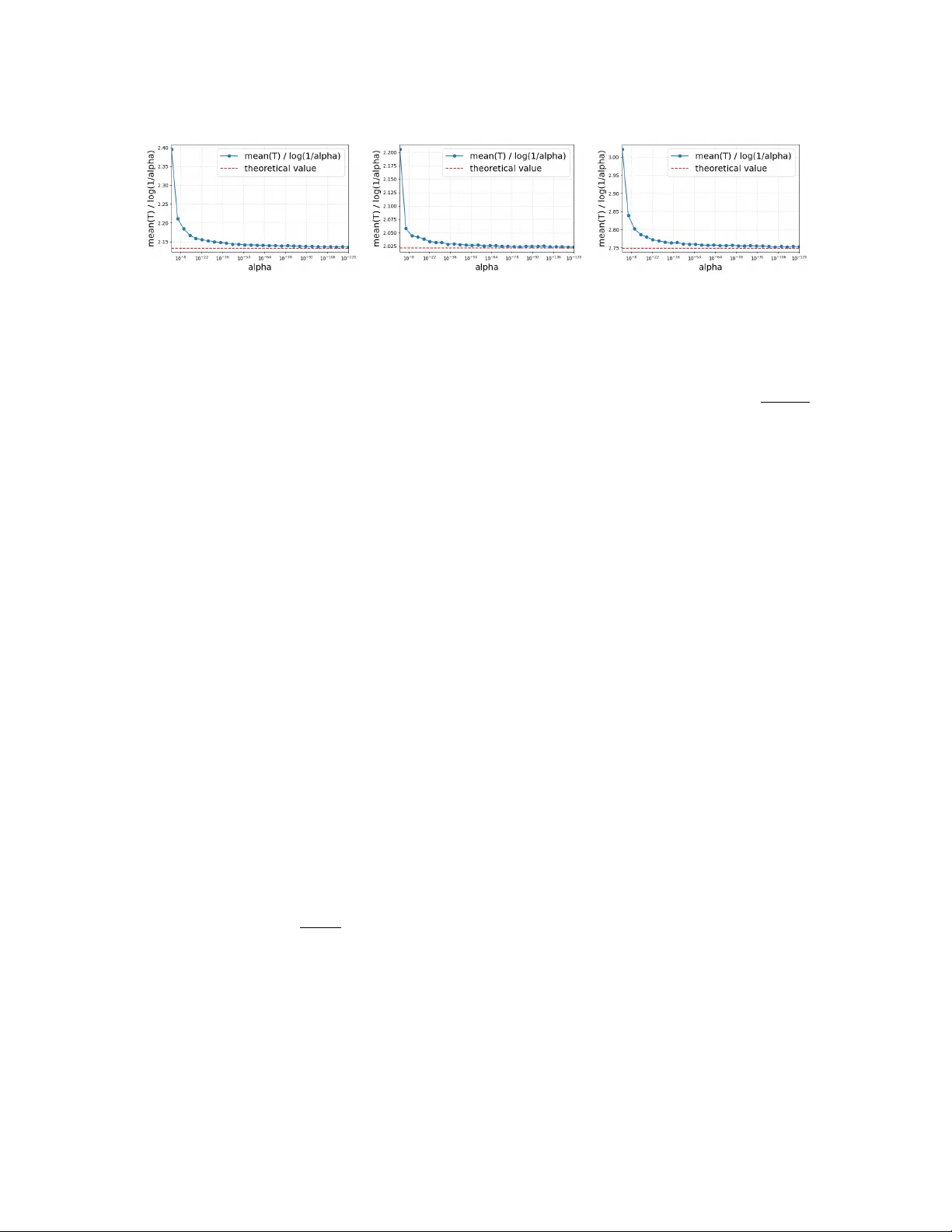
T o wards An ytime-V alid Statistical W atermarking Baihe Huang * Eric Xu † Kannan Ramchandran ‡ Jiantao Jiao § Michael I. Jordan ¶ Abstract The proliferation of Lar ge Language Models (LLMs) necessitates efﬁcient mech- anisms to distinguish machine-generated content from human text. While statistical watermarking has emer ged as a promising solution, existing methods suf fer from two critical limitations: the lack of a principled approach for selecting sampling distri- butions and the reliance on ﬁxed-horizon hypothesis testing, which precludes v alid early stopping. In this paper , we bridge this gap by de veloping the ﬁrst e-v alue-based watermarking framew ork, Anchor ed E-W atermarking , that uniﬁes optimal sampling with anytime-v alid inference. Unlike traditional approaches where optional stopping in validates T ype-I error guarantees, our frame work enables v alid, an ytime-inference by constructing a test supermartingale for the detection process. By le veraging an anchor distribution to approximate the tar get model, we characterize the optimal e-v alue with respect to the worst-case log-gr owth rate and deriv e the optimal expected stopping time. Our theoretical claims are substantiated by simulations and e valuations on es- tablished benchmarks, sho wing that our frame work can signiﬁcantly enhance sample ef ﬁciency , reducing the av erage token b udget required for detection by 13-15% relativ e to state-of-the-art baselines. 1 Intr oduction The re volutionary success of Lar ge Language Models (LLMs) at generating human-like texts (Bro wn et al., 2020; Bubeck et al., 2023; Cho wdhery et al., 2023) has raised se veral societal concerns re garding the misuse of LLM outputs. Unregulated LLM outputs pose risks ranging from the contamination of future training corpora (Shumailo v et al., 2023; Das et al., 2024) to the propagation of disinformation (Zellers et al., 2019; V incent, 2022) and academic misconduct (Jarrah et al., 2023; Milano et al., 2023). Consequently , there is an * baihe huang@berkeley.edu . Univ ersity of California, Berkeley . † erx@berkeley.edu . Uni versity of California, Berkele y . ‡ kannanr@berkeley.edu . Uni versity of California, Berkele y . § jiantao@eecs.berkeley.edu . Uni versity of California, Berkele y . ¶ jordan@cs.berkeley.edu . Uni versity of California, Berkele y . 1 urgent need for reliable detection mechanisms capable of distinguishing LLM-generated text from human-authored content. T o address this challenge, Aaronson (2022a) and Kirchenbauer et al. (2023) propose sta- tistical watermarking as a theoretically-grounded method to distinguish machine-generated content from a target distribution. These methods operate by injecting statistical signals into the generated texts in the decoding phase of LLMs. Mechanistically , the watermark generator couples the output tokens by a sequence of pseudorandom seeds. During detection, the detector reconstructs the seeds and performs a hypothesis test to check the dependence between the seeds and the observed tokens. This formulation allo ws the detection prob- lem to be treated as a rigorous statistical hypothesis test (Huang et al., 2023) where the detection po wer and sample complexity are gov erned by the randomness in the target distri- bution. V arious designs for the underlying seed distrib utions hav e been explored, such as binary (Christ et al., 2023), exponential (Kuditipudi et al., 2023), and Gaussian (Block et al., 2025). Recently , Huang et al. (2025) advanced the concept of using an auxiliary open-source model as an anchor to generate random seeds and coupling them with tokens via speculati ve decoding (Le viathan et al., 2023). This approach is motiv ated by the theoretical insight that watermarking achie ves the optimal po wer when the seed distribution approximates the tar get distribution (Huang et al., 2023). By exploiting the distributional proximity between modern LLMs, anchor-based methods hav e shown promise in impro ving both detection efﬁcienc y and rob ustness to remo ving-attacks (Piet et al., 2023). Empirically , watermarked te xts can be detected within short token horizons ( < 100 tokens) and high success rate (nearly 50% under paraphrasing) under v arious attacks. Despite these successes, state-of-the-art watermarking remains constrained by two fundamental limitations. First, the design of generation and detection schemes lacks a unifying guiding principle. Huang et al. (2025) utilize a hashed green-red-list seed adapted from Kirchenbauer et al. (2023), b ut this heuristic lacks rigorous justiﬁcation. What is needed is a characterization of optimal generation and detection schemes under gi ven anchor distributions. Second, there e xists a methodological disconnect between generation and detection. While text generation is inherently autoregressi ve and v ariable in length, current detection paradigms are ﬁxed-horizon and ad hoc . In practice, for example, a detector may wish to process a stream of tokens and stop as soon as conﬁdence is high. Ho we ver , with the standard statistical paradigm based on p-v alues, it is not allo wed to continuously monitor the test statistic and decide when to stop based on the current value—this is kno wn as “p-hacking” and it in validates the T ype-I error guarantee. This inability to perform post-hoc sequential analysis se verely limits detection ef ﬁciency . These gaps highlight a critical research challenge: How can we design pr ovably ef ﬁcient watermarking schemes lever aging anchor distributions that allow for valid early stopping? In this w ork, we pro vide the ﬁrst formal resolution to this question. W e formulate the problem of Anchor ed E-W atermarking , where both the generator and detector share access to an anchor distrib ution p 0 , aiming to watermark a f amily of distrib utions in the δ -proximity 2 of p 0 . Departing from classical p-value analysis, we adopt e-values as the central detection paradigm. E-values (V ovk, 1993; Shafer et al., 2011; V ovk & W ang, 2021) are nonnegati ve random v ariables E satisfying E H 0 [ E ] ≤ 1 under the null. Unlike p-v alues, e-v alues arise from supermartingales, and it is therefore possible to preserve T ype-I error guarantees under optional stopping based on ongoing analysis of data. W e analyze the optimal e-value for watermark detection with respect to the worst-case log-gro wth rate (Kelly, 1956) and the expected stopping time (Gr ¨ unwald et al., 2020; W audby-Smith et al., 2025), thus fully characterize the a verage per-step gro wth rate of e vidence and sample efﬁcienc y . Our main theoretical contributions are summarized informally as follo ws: Theorem 1.1 (Informal v ersion of Theorem 4.1 and Theorem 4.3) . The optimal worst-case log-gr owth r ate E H 1 [log E ] under the alternative H 1 is given by: J ∗ = h +  1 − δ 2  log  1 − δ 2  + δ 2 log  δ 2( n − 1)  , wher e h = H ( p 0 ) is the Shannon entr opy of the anchor distribution p 0 and δ > 0 is a r ob ustness tolerance parameter . Furthermor e, the optimal e xpected stopping time to ac hieve a T ype-I err or α scales as log(1 /α ) J ∗ . T o the best of our knowledge, this work represents the ﬁrst application of e-values to the domain of statistical watermarking. By enabling valid sequential testing, our framew ork signiﬁcantly improv es detection efﬁcienc y , allo wing the system to ﬂag machine-generated text with fe wer tokens than ﬁxed-horizon counterparts. W ith the ability to early-stop, this sequential paradigm enhances robustness against adaptiv e attacks: because the detector can terminate immediately upon accumulating suf ﬁcient evidence, the w atermark remains ef fective e ven if the attacker perturbs the text heavily in later segments (post-stopping). Consequently , our approach offers a theoretically rigorous and practically superior alterna- ti ve to existing heuristic detection methods. Through e xperiments on real watermarking benchmark (Piet et al., 2023), we show that the theoretical scheme implied by Theorem 1.1 achie ves consistently higher sample ef ﬁciency than state-of-the-art methods, reducing the token consumption by 13-15% across v arious temperature settings. 1.1 Related works Statistical watermarking. W atermarking of fers a white-box provenance mechanism for detecting LLM-generated te xt (T ang et al., 2023), complementing post-hoc detectors and prov enance tools developed for neural te xt generation (Zellers et al., 2019). Classical digital watermarking and steg anography provide a broad toolbox for embedding and extracting imperceptible signals under benign or adv ersarial channel edits (Cox et al., 2007). Early works in NLP literature studied watermarking and tracing of text via editing or synonym substitutions (V enugopal et al., 2011; Rizzo et al., 2019; Abdelnabi & Fritz, 2021; Y ang et al., 2022; Kamaruddin et al., 2018). In contrast, modern statistical (a.k.a. generati ve) watermarking (Aaronson, 2022a; Kirchenbauer et al., 2023) injects a secret, testable dis- tributional bias into the sampling process, and detects this bias via hypothesis testing on 3 the generated token sequence. A rapidly gro wing theory studies ef ﬁciency and optimality of watermarking tests and encoders: results include ﬁnite-sample guarantees, information- theoretic limits, and constructions that are distortion-free or unbiased (Huang et al., 2023; Zhao et al., 2023; Li et al., 2024; Block et al., 2025; K uditipudi et al., 2023; Hu et al., 2023; Xie et al., 2025). Neg ative and hardness results highlight fundamental limitations against adapti ve or distrib ution-matching adversaries (Christ et al., 2023; Christ & Gunn, 2024; Golowich & Moitra, 2024), motiv ating alternativ e design considerations such as distribution-preserving and public-ke y schemes (W u et al., 2023; Liu et al., 2023; F airoze et al., 2023). Empirical robustness is commonly assessed under paraphrasing, editing and translation, with recent work studying cross-lingual failure modes and defenses (He et al., 2024b), and benchmarks/frame works such as MarkMyW ords and scalable pipelines for watermark ev aluation and deplo yment (Piet et al., 2023; Zhang et al., 2024; Lau et al., 2024; Dathathri et al., 2024). Finally , a complementary line of work lev erages semantic structure and auxiliary models to boost detection po wer under benign distrib utional structure, including semantic/paraphrastic watermarks and speculati ve-sampling-based schemes (Ren et al., 2024; Liu & Bu, 2024; Hou et al., 2024b,a; Fu et al., 2024; Huang et al., 2025; Le viathan et al., 2023). Our anchored e-value approach b uilds on these works by explicitly treating detection as anytime-v alid sequential testing (Chen & W ang, 2024), and by allo wing model-assisted calibration under distribution shift (Huang et al., 2025; He et al., 2024a, 2025). E-values and sequential h ypothesis testing. Sequential hypothesis testing studies infer- ence procedures that remain valid under data-dependent stopping and streaming data (W ald, 1947; Robbins, 1952; Breiman, 1961). Classical likelihood-ratio and p -v alue based methods can fail under optional stopping or composite hypotheses, motiv ating the use of nonnegati ve supermartingales / test martingales whose stopped values are valid evidence measures (Shafer et al., 2011; V ovk & W ang, 2021; Shafer, 2021; Gr ¨ unwald et al., 2020; Ramdas et al., 2023). The resulting e-values and e-pr ocesses unify betting scores, likelihood ratios, and (stopped) Bayes factors. Additionally , e-values and e-processes support modular operations such as merging and calibration (V ovk & W ang, 2021; Ramdas & W ang, 2025). This frame work has enabled principled notions of po wer and optimality , including log-/gro wth-rate criteria and sharp asymptotic rates for broad classes of betting-based tests (Gr ¨ unwald et al., 2020; W audby-Smith et al., 2025). E-values also interact fruitfully with multiple testing and online testing, yielding e-v alue analogues of the BH and wealth-based procedures and their extensions to structured settings (W ang & Ramdas, 2022; Ramdas et al., 2017, 2018, 2019). Recent work further broadens the reach of e-values to new ML settings, such as conformal prediction and sequential monitoring of strategic systems (Gauthier et al., 2025, 2026; Aolaritei & Jordan, 2025), and connects e-v alues to model-assisted ef ﬁciency gains via prediction-po wered inference (W asserman et al., 2020; Csillag et al., 2025). Our work draws on these foundations to construct e-values tailored to watermark detection which ensures v alidity under arbitrary stopping rules and enables sequential e vidence accumulation in practical prov enance audits. 4 2 Pr eliminaries 2.1 Statistical watermarking Statistical w atermarking for Large Language Models (LLMs) provides a probabilistic frame work for distinguishing machine-generated text from human-written text. Unlike post-hoc detection methods that rely on classiﬁers trained on model artifacts, watermarking acti vely embeds a statistical signal into the generation process. This signal is designed to be imperceptible to humans yet statistically signiﬁcant to an algorithmic detector possessing a secret ke y . Statistical watermarking as a hypothesis testing pr oblem. Formally , statistical water- marking is cast as a hypothesis testing problem. Let q denote the target distribution over the sample space V , and let S represent the space of pseudorandom seeds. The watermark- ing protocol modiﬁes the standard decoding mechanism of the LLM such that the output tokens V ∈ V and the pseudorandom seeds S ∈ S are sampled jointly from a watermarked distribution P W . The detection task seeks to determine if a gi ven observ ed text v was generated by the watermarked model: D : V × S → { W atermarked , Unwatermark ed } . This reduces to testing for independence between the tok ens v and the seeds s reconstructed via the detector’ s key . W e deﬁne the null and alternati ve hypotheses as follo ws (Huang et al., 2023): • Null hypothesis H 0 : The text v is generated independently of the seeds s (e.g., by a human or an unwatermarked model). • Alternati ve h ypothesis H 1 : The text v and seeds s are sampled from the joint watermarked distrib ution P W , implying they come from the w atermarked model. It is pertinent to distinguish this distributional watermarking approach from classical instance-le vel watermarking techniques applied to static media, such as images or audio Cox et al. (2007). While classical methods embed a signature into a speciﬁc, ﬁxed outcome (post-generation), statistical watermarking modiﬁes the stochasti c sampling process itself, ensuring that an y realization from the model carries the statistical evidence of its origin without requiring rigid alterations to the ﬁnal output. Statistical guarantees. A rob ust watermarking scheme is characterized by its ability to provide three fundamental guarantees. First, to preserv e generation quality and ensure watermark ed content remains indistin- guishable from ordinary samples, the distance (e.g., KL-di ver gence) between the water- marked distrib ution P W and the original tar get distribution q must be minimized. Ideally , we seek a scheme that introduces zero distributional shift (Hu et al., 2023). 5 Deﬁnition 2.1 (Distortion-free) . A watermark is considered distortion-fr ee (or unbiased) if the outcome marginal of the watermark ed distribution P W matches the target distrib ution q . Formally , a distortion-free watermark satisﬁes: X s ∈S P W ( A, s ) = q ( A ) , ∀ A ⊆ V . Second, it is often required in practice that the detector operates without access to the watermarked distrib ution since the underlying model’ s parameters are generally unkno wn to the detector . This means that the detection scheme needs to be designed for a family of tar get distrib utions in a model-agnostic way (Kuditipudi et al., 2023), leading to the ne xt concept. Deﬁnition 2.2 (Model-agnosticity) . A watermark is model-agnostic if the seed-marginal of P W is chosen independently of the target distrib ution q . That is, the distribution of seeds S does not depend on the model’ s logits. Third, the reliability of the watermark is quantiﬁed by standard statistical error rates. The T ype I err or (false positi ve rate) measures the probability of incorrectly identifying non-watermarked te xt (e.g., human-written) as watermarked. Giv en the high stakes of false accusations (e.g., in academic integrity), this error must be bounded by a small signiﬁcance le vel α : P H 0 ( D ( V , S ) = W atermarked ) ≤ α. The T ype II err or (false negati ve rate) measures the probability that w atermarked text f ails to be detected. Minimizing this error is equiv alent to maximizing the statistical power of the test. For a target error rate β , we require: P H 1 ( D ( V , S ) = Unwatermarked ) ≤ β . 2.2 Sequential hypothesis testing and e-v alues Consider a measurable space (Ω , F ) and a family of probability distributions P . W e are interested in testing a null hypothesis H 0 : P ∈ P 0 ⊂ P against an alternativ e H 1 : P ∈ P 1 = P \ P 0 . An e-value is a random v ariable whose expectation is bounded by unity under the null hypothesis (V ovk & W ang, 2021). Deﬁnition 2.3 (E-v alue) . A nonnegati ve random v ariable E is an e-v alue for H 0 if for all P ∈ P 0 , E P [ E ] ≤ 1 . Intuiti vely , an e-v alue represents the amount of wealth a gambler would ha ve after betting against the null hypothesis, in a g ame where the game is fair or unf av orable under H 0 , and starting with an initial wealth of one. On the other hand, if E becomes lar ge, this suggests that the null hypothesis is unlikely to be true. 6 Sequential evidence and stopping time guarantees. The primary advantage of e-v alues lies in their beha vior re garding stopping times. In a sequential setting, we are gi ven a ﬁltration ( F t ) t ≥ 0 and construct a sequence of e-v alues ( E t ) t ≥ 0 . If ( E t ) t ≥ 0 is a nonneg ative supermartingale with respect to the null distributions (often called a test martingale ), it allo ws for anytime-valid inference. This property deri ves from V ille’ s inequality , a time- uniform generalization of Marko v’ s inequality . Theorem 2.4 (V ille’ s inequality) . Let ( E t ) t ≥ 0 be a nonne gative supermartingale with r espect to P ∈ P 0 such that E 0 ≤ 1 . Then for any α ∈ (0 , 1) , P  ∃ t ≥ 0 : E t ≥ 1 α  ≤ α . This result guarantees that a researcher can track the e-v alue process continuously and stop at any data-dependent time τ (a stopping time) while maintaining T ype-I error control. Speciﬁcally , E P [ E τ ] ≤ 1 holds for any stopping time τ (possibly unbounded), a kind of guarantee which is not av ailable for p-v alues. 3 Pr oblem Formulation In this section, we formulate the problem of Anc hored E-W atermarking . Similar to statistical watermarking, the goal is to embed statistical signals into samples from a target distribution to enable detection. Howe ver , in Anchored E-W atermarking, the generator and the detector share access to an anchor distrib ution that serves as a rob ust a priori estimate of the tar get distribution. This setting is common in practice; for example, when watermarking Large Language Models or image generators, the tar get distribution is known to be human language or natural images, respecti vely . Consequently , watermarking ef ﬁcacy can be impro ved by le veraging this structure. Besides, Anchored E-W atermarking uses e-v alues for detection, thus enjoying impro ved ef ﬁciency in sequential testing. In the following, we introduce the speciﬁc components of Anchored E-W atermarking. Anchor distribution. In the Anchored E-W atermarking framework, we assume that both the generator and the detector share access to an anchor distribution p 0 ∈ ∆( V ) , which is in the same probability simple x as the target distrib ution q . This p 0 serves as the best a priori estimate of the target distribution. For instance, in the context of watermarking Large Language Models (LLMs), p 0 could be an open-source, smaller-scale LLM such as Qwen3- 8B (T eam, 2025). Lev eraging its role as a known reference, we designate p 0 as the marginal distribution for the w atermark signal (or random seed), denoted as s . Therefore, the seed space S is equal to V in our frame work. Throughout the paper , we assume p 0 satisﬁes the condition inf v ∈V p 0 ( v ) > δ for a positi ve rob ustness tolerance parameter δ . This condition ensures p 0 has enough randomness as required for watermarking (Aaronson, 2022a) and that the δ -neighborhood deﬁned belo w is a strict subset of the probability simplex. 7 T arget distribution. The target distrib ution q ∈ ∆( V ) represents the desired distrib ution from which (watermarked) output samples v are generated. Consistent with the deﬁnition of the anchor , we premise that q remains suf ﬁciently proximal to p 0 . Formally , we assume q resides within the δ -neighborhood of the anchor: Q ( p 0 , δ ) = { q ∈ ∆( V ) : ∥ q − p 0 ∥ 1 ≤ δ } . Here ∥ · ∥ 1 is the ℓ 1 distance and the radius δ > 0 represents a robustness tolerance parameter that controls how the true target distrib ution q can deviate from the anchor . This assumption holds for most practical statistical w atermarking scenarios; for example, in the LLM domain, high-performing models tend to con verge towards the same underlying distribution of natural language, resulting in lo w statistical div ergence between them. Generator . The objectiv e of the generator is to sample an output v from the target distri- bution q while embedding a statistical signal s . T o achiev e this, the generator constructs a joint distrib ution (or coupling) w ov er v and s , subject to the constraint that the marginals recov er the target and anchor distributions, respecti vely . The feasible set of valid couplings is deﬁned as: P ( p 0 , q ) =  w ∈ ∆( V × V ) : X s ∈V w ( v , s ) = q ( v ) , X v ∈V w ( v , s ) = p 0 ( s )  . Note that the generator has access to q , as is common in practice (e.g., when the generator is a service provider). During generation, the system samples the outcome v and the signal s jointly from w . This procedure ensures that the mar ginal distrib ution of the outcome v is unbiased (satisfying Theorem 2.1), while the watermark signal is embedded within the statistical dependency between v and s . E-value. In the detection phase, the detector recei ves an outcome-signal pair ( v , s ) and computes an e-value e ( v , s ) ≥ 0 . The objectiv e is to distinguish between the following hypotheses: H 0 : v and s are sampled independently , H 1 : ( v , s ) are sampled from the joint coupling w . The detector rejects the null h ypothesis if e ( v , s ) > 1 /α . T o guarantee a T ype-I error rate of at most α , the e xpectation of the e-v alue under the null hypothesis must be bounded by 1 . Adhering to the model-agnostic constraint (Theorem 2.2), the scoring function e ( · , · ) must be deﬁned prior to observing the speciﬁc target distribution q . The design of the e-v alue relies solely on the constraint that the tar get distribution lies within the anchor’ s neighborhood, i.e., q ∈ Q ( p 0 , δ ) . Consequently , to ensure v alidity , the e-value must satisfy the expectation bound uniformly across the entire uncertainty set Q : sup q ∈Q ( p 0 ,δ ) E v ∼ q,s ∼ p 0 [ e ( v , s )] ≤ 1 . (1) W e let E denote the set of all nonnegati ve functions e : V × V → R satisfying Eq. (1). 8 3.1 Rob ust log-optimality While the deﬁnition of an e-value ensures validity (safety) under the null, it does not guarantee po wer (growth) under the alternativ e. T o reject H 0 ef fectively , we desire the e-v alue to be large when the data is generated from the alternati ve distrib ution H 1 . The standard criterion for selecting an e-v alue is log-optimality , often referred to as the “K elly criterion” in the ﬁnance literature (Kelly, 1956). This approach seeks to maximize the expected logarithmic gro wth rate of e vidence against the null, under the alternative. For simple hypotheses where P 0 = { P } and P 1 = { Q } , the likelihood ratio e ∗ = dQ dP is log-optimal, such that E Q [log e ∗ ] ≥ E Q [log e ] for any v alid e-v alue e . In Anchored E-W atermarking, the alternati ve is deﬁned by the joint coupling w con- structed by the generator . Ho wev er , since the target distribution q lies in a set Q ( p 0 , δ ) that is unknown to the detector (i.e., the designer of the e-value), we must optimize the worst-case log-gro wth rate ov er arbitrary q ∈ Q ( p 0 , δ ) . This giv es rise to the following robust log-optimality problem. Problem 3.1 (Robust log-optimality) . An e-v alue e is r ob ust log-optimal in Anchored E-W atermarking if it optimizes the follo wing objectiv e: sup e ∈E inf q ∈Q ( p 0 ,δ ) sup w ∈P ( p 0 ,q ) X v ,s ∈V w ( v , s ) · log e ( v , s ) . (2) In this formulation, the objectiv e P w ( v , s ) log e ( v , s ) represents the log-gro wth rate un- der the alternati ve. The inner maximization sup w ∈P ( p 0 ,q ) reﬂects the generator’ s optimization of the coupling w gi ven kno wledge of q ; the minimization inf q ∈Q ( p 0 ,δ ) enforces rob ustness against the worst-case tar get distribution in the f amily; and the outer maximization sup e ∈E seeks the optimal detector without access to q subject to model-agnostic y (Theorem 2.2). Remark 3.2 (Relationship to gro wth rate optimality in the worst case (GR O W) (Gr ¨ unwald et al., 2020)) . GR O W studies the worst-case optimal e xpected capital gr owth r ate under composite null P 0 and alternative P 1 : GR OW( P 1 ) = sup E ∈E ( P 0 ) inf θ ∈P 1 E P θ [ l og E ] , wher e E ( P 0 ) is the set of all valid e-values for the null P 0 . Therefor e, our pr oblem in Eq. (2) can be seen as generalizing GR O W into an ‘active’ scenario wher e a generator (corr esponding to sup w ∈P ( p 0 ,q ) ) seeks to maximizes the power after the worst-case hypothesis selection inf θ ∈P 1 . Note that by designing the coupling w , the gener ator essentially alters the alternative, so our pr oblem can not be r educed to GR O W even if the watermark generator is ﬁxed. 9 3.2 Stopping time While Theorem 3.1 addresses the one-step gro wth rate, it remains to analyze the sample complexity of the framework. In the context of sequential hypothesis testing, sample ef ﬁciency is characterized by the stopping time τ α = inf { n ∈ Z + : W n ≥ log (1 /α ) } under the alternati ve, where W n = n X t =1 log e ( v t , s t ) , is the accumulated wealth process. This quantity represents the number of samples required to reject the null hypothesis. W e consider a stochastic process µ ( A , G ) gov erned by the interaction between an adversary A and a generator G . At each step t ∈ Z + : • The adversary A selects q t ∈ Q ( p 0 , δ ) based on the e-v alue e and the history ( v 1 , s 1 ) , . . . , ( v t − 1 , s t − 1 ) ; • The generator G speciﬁes the joint coupling w t gi ven q t and p 0 , and draws the sample ( v t , s t ) ∼ w t . Due to the adaptive nature of the adversary , the outcome sequence v 1 , v 2 , . . . may be generated autoregressi vely , conditional on pre vious outcomes. This formulation extends the i.i.d. setting of Huang et al. (2023) to arbitrary dependent distrib utions. In this setting, we write the stopping time as τ α ( e ) to highlight the dependence on the e-value e . In the context of sequential testing (Breiman, 1961; Chugg et al., 2023; Shekhar & Ramdas, 2023; Kaufmann & K oolen, 2021; W audby-Smith et al., 2025), the expected stopping time E [ τ α ] typically scales linearly with log(1 /α ) , modulated by an information-theoretic quantity capturing the complexity of the testing problem. Therefore, we are e xplicitly interested in the follo wing question: Problem 3.3 (Sample ef ﬁciency) . For any e-v alue e satisfying the constraint in Eq. (1) , deﬁne its sample complexity by SC( e ) = sup A inf G lim inf α → 0 E µ ( A , G ) [ τ α ( e )] log(1 /α ) . W e are interested in identifying the e-v alue that minimizes this sample complexity . Note that this formulation is stronger than the classical expected stopping time because we allo w the adversary to alter the distribution at each time step. This implies that samples are not generated in an i.i.d. fashion, a distinction crucial for applications such as the watermarking of autore gressiv e language models. 4 Theor etical Results In this section, we answer the questions posed in the pre vious section. W e ﬁrst deri ve the optimal detector for the single-step decision problem and then extend this analysis to the 10 sequential setting to characterize the fundamental limit of sample ef ﬁciency . Let n denote the cardinality of the sample space V and e v denote the one-hot vector (i.e., Dirac measure) that assigns mass 1 to v ∈ V . 4.1 Optimal log-gr owth rate W e begin by solving the robust log-optimality problem deﬁned in Theorem 3.1. The follo wing theorem provides a closed-form solution for both the optimal e-v alue and the worst-case-optimal generator beha vior . Theorem 4.1 (Log-gro wth rate) . The optimal e-value that solves the objective in Eq. (2) is given by: e ∗ ( v , s ) = ( 1 − δ / 2 p 0 ( s ) , s = v , δ 2( n − 1) p 0 ( s ) , s  = v , (3) wher e n = |V | . Furthermor e, for any targ et distrib ution q ∈ Q ( p 0 , δ ) decomposed as q = P k i =1 λ i q i wher e q i = p 0 + δ 2 · ( e v i − e s i ) , v i  = s i ∈ V ar e the extr eme points of Q ( p 0 , δ ) , the optimizer of the inner maximization pr oblem (the generator’ s optimal coupling) is: w ∗ = k X i =1 λ i ·  δ 2 · ( e v i e ⊤ s i − e s i e ⊤ s i ) + diag ( p 0 )  . (4) The optimal r ob ust log-gr owth r ate is equal to: J ∗ = h +  1 − δ 2  log  1 − δ 2  + δ 2 log  δ 2( n − 1)  , (5) wher e the term h = H ( p 0 ) is the Shannon entr opy of the anc hor distribution p 0 . The result in Equation (5) fundamentally express the optimal growth rate of e-v alues in Anchored E-W atermarking. The ﬁrst term is the entropy of the anchor distrib ution, which mathematically formalizes the intuition that watermarking is inherently easier for distribu- tions with high entrop y . The second term can be written as − H ( ν δ ) , the ne gativ e entropy of the categorical distribution ν δ = (1 − δ / 2 , δ / (2( n − 1)) , . . . , δ / (2( n − 1))) ∈ ∆([ n ]) , which is a decreasing function of δ . This explicitly characterizes the power -robustness tradeof f determined by the tolerance parameter δ . Written as H ( p 0 ) − H ( ν δ ) , the optimal log-gro wth rate is the achiev ed information rate of an Additiv e Noise Channel Y = X ⊕ Z where X ∼ p 0 , Z ∼ ν δ . Remark 4.2 (Relationship to SEAL (Huang et al., 2025)) . SEAL pr oposes to use a smaller language model as p 0 and speculative decoding as the gener ator . Note that the optimizer of the inner pr oblem given in Eq. (4) is e xactly the maximal coupling given by speculative decoding. Ther efor e, Theor em 4.1 conﬁrms that the choice of generator in Huang et al. (2025) is optimal. Howe ver , the optimal detector given by Eq. (3) is differ ent fr om the detection rule in SEAL: this gap is corr oborated by e xperiments in Section 5.2. 11 4.2 Sample efﬁciency Having characterized the one-step optimal growth rate, we no w analyze the long-term performance of the watermark in a sequential setting. The following theorem connects the log-gro wth rate J ∗ to the sample comple xity required to reject the null hypothesis against an adapti ve adversary . Theorem 4.3 (Expected stopping time) . Let µ ( A , G ) be the stochastic pr ocess deﬁned in Theor em 3.3 and τ α ( e ) be the stopping time under e-value e . Let J ∗ be the optimal rate deﬁned in Eq. (5) . W e have the following bounds on sample efﬁciency: • Lower bound (con verse): F or any valid e-value e ∈ E : sup A inf G lim inf α → 0 E µ ( A , G ) [ τ α ( e )] log(1 /α ) ≥ 1 J ∗ . • Upper bound (achievability): F or the optimal e-value e ∗ deﬁned in Theor em 4.1: sup A inf G lim inf α → 0 E µ ( A , G ) [ τ α ( e ∗ )] log(1 /α ) = 1 J ∗ . Theorem 4.3 establishes 1 /J ∗ as the fundamental information-theoretic limit of sample complexity for Anchored E-W atermarking. It demonstrates that the e-value e ∗ deri ved from the one-step greedy optimization is not only locally optimal but also globally optimal for sequential testing. Crucially , this optimality holds e ven against an adapti ve adv ersary that can v ary the target distrib ution at e very step, pro vided the distribution remains within the δ -neighborhood of the anchor . Remark 4.4 (Relationship with the rates in Huang et al. (2023)) . Huang et al. (2023) shows that the minimum number of samples r equir ed to watermark with T ype I err or α scales as log(1 /α ) · log(1 /h ) h , wher e h is the averag e entr opy per token. While our rate log(1 /α ) h has the same scaling in terms of α , its dependence on the entr opy h is impr oved. This is because Huang et al. (2023) study an asymptotic r egime wher e h → 0 , while we ﬁx an anchor distribution with lower bounded entr opy arising fr om the condition inf v ∈V p ( v ) > δ . 5 Experiments 5.1 Synthetic experiments In this section, we v erify our theoretical results with synthetic experiments on a f amily of simple target distributions. Here, we consider the two-token case where |V | = 2 and for simplicity of notation, we let V = { 0 , 1 } . Any anchor distribution we consider belongs to a one-parameter Bernoulli family p 0 =  p 1 − p  for p ∈ (0 , 1) . 12 (a) p = 0 . 2 (b) p = 0 . 5 (c) p = 0 . 75 Figure 1: Simulation of the two-token case for the log growth problem in Eq. (2) . Three separate anchor distrib utions are used each with parameter δ = 0 . 01 . W e solve the simpliﬁed maxmin problem using the CLARABEL interior point method solver which is run for 30 steps. The theoretical optimum is computed as in Eq. (5). Log-gro wth optimality . W e solve the optimization problem in Eq. (2) numerically and compare the objecti ve curve with the theoretical prediction. W ith n = 2 , the problem can be simpliﬁed to the follo wing maxmin problem: sup e X v p 0 ( v ) log e ( v , v ) + δ 2 min  log e (0 , 1) e (1 , 1) , log e (1 , 0) e (0 , 0)  subject to the constraint in Eq. (1) with Q ( p 0 , δ ) replaced with the set of vertices Q ext ( p 0 , δ ) := { p 0 ± δ 2 ( e 0 − e 1 ) } . Using the CLARABEL interior point method solver Goulart & Chen (2024), we obtain the results in Fig. 1. W e choose δ = 0 . 01 and p = 0 . 2 , 0 . 5 , 0 . 75 corre- sponding to three separate anchor distributions p 0 . For each p 0 , we cold start the IPM solver and run it for 30 steps with maximum allo wed step size 0 . 99 . W e observe that our numerical solution to Eq. (2) con ver ges to the proposed theoretical v alue in Eq. (5) , hence v erifying our theoretical results in the two-token case. Stopping time. In this setting, we simulate sequential testing with the optimal e-value e ∗ , as in Eq. (3) . Follo wing Theorem 4.1, we let A ∗ be the adversary that chooses q t = q ∗ for all t and G ∗ be the generator that selects w t = w ∗ in response to A ∗ for all t . Under this setting, we simulate the stopping time over se veral α v alues to obtain the results in Fig. 2. Here, we choose the parameters δ = 0 . 1 and p = 0 . 2 , 0 . 5 , 0 . 75 . For each anchor p 0 , we compute the corresponding q ∗ , w ∗ , and e ∗ using the closed-form equations in Theorem 4.1. W e select 30 v alues of α e venly log-spaced from 10 − 2 to 10 − 120 . F or each α , we compute 10000 stopping-times by generating sequences ( V t , S t ) t ≥ 1 ∼ w ∗ and computing the resulting log e ∗ ( V t , S t ) . W e then average the stopping times to form an estimate of E µ ( A ∗ , G ∗ ) [ τ α ( e ∗ )] . In Fig. 2, we plot our estimates of E µ ( A ∗ , G ∗ )[ τ α ( e ∗ )] / (log(1 /α )) which sho w that as α ↓ 0 , the estimates con ver ge to the theoretical rate of 1 /J ∗ , thereby v alidating the result in Theorem 4.3. 13 (a) p = 0 . 2 (b) p = 0 . 5 (c) p = 0 . 75 Figure 2: Simulation of the two-token case for the stopping time problem SC ( e ∗ ) . W e simulate for three dif ferent anchor distributions p 0 =  p 1 − p  with δ = 0 . 1 and estimate av erage stopping times E [ τ α ] for α v alues ranging from 10 − 2 to 10 − 120 . Each E [ τ α ] is estimated by simulating 10000 stopping times τ α . The plots above display graphs of E [ τ α ] log(1 /α ) with red dashed lines equal to 1 /J ∗ where J ∗ is as in Eq. (5) . W e observe that con ver gence to the theoretical optimum is obtained for suf ﬁciently small α . 5.2 Experiments on r eal data W e e valuate the performance of our w atermarking scheme in Theorem 4.1 by comparing it with se veral baselines on a real watermarking task. Setup. W e select Llama2-7B-chat (T ouvron et al., 2023) with temperature 0 . 7 as target distribution (i.e., the model to be watermark ed) and Phi-3-mini-128k-instruct (Abdin et al., 2024) as the anchor distrib ution. W e ev aluate our watermark using the M A R K M Y W O R D S benchmark (Piet et al., 2023), which is an open-source benchmark designed to ev aluate symmetric ke y watermarking schemes. M A R K M Y W O R D S generates 300 outputs spanning three tasks—book summarization, creati ve writing, and news article generation—which mimic potential misuse scenarios. Then, watermarked outputs under go a set of transformations mimicking realistic user pertur- bation or attacks: (1) character-le vel perturbations (contractions, e xpansions, misspellings and typos); (2) word-le vel perturbations (random remov al, addition, and swap of words in each sentence, replacing words with synon yms); (3) text-le vel perturbations (paraphrasing, translating the output to another language and back). Detection is run in a sequential test set- ting with early stopping. For baseline methods, we apply Bonferroni corrections to preserve anytime valid T ype-I error guarantees: let p k denote the p-v alue at time step k ∈ Z + , reject at the ﬁrst time p k < α k ( k +1) . Results. In this section, we present a comprehensi ve comparison of our m ethod against these baselines in terms of quality and size. Quality measures the utility of the watermarked text. It is computed using Llama-3 (Dubey et al., 2024) with greedy decoding as a judge model, and ranges from zero to one. Size represents the median number of tokens required to detect the w atermark at a gi ven p-v alue, computed ov er a range of perturbations listed abov e. 14 All experiments enforce a T ype-I error constraint of α = 0 . 02 . Lower v alues indicate higher ef ﬁciency . W e compare against ﬁ ve state-of-the-art w atermarking schemes: “Distribution Shift” (Kirchenbauer et al., 2023), “Exponential” (Aaronson, 2022b), “Binary” (Christ et al., 2023), “In verse T ransform” (Kuditipudi et al., 2023), and “SEAL ” (Huang et al., 2025). Scheme Quality ( ↑ ) Size ( ↓ ) Exponential 0.907 ∞ In verse T ransform 0.917 734.0 Binary 0.919 ∞ Distribution Shift 0.912 145.0 SEAL 0.901 84.5 Theorem 4.1 0.919 72.0 T able 1: Comparison of our e-value-based watermarking scheme in Theorem 4.1 with baselines across quality and size. W e report the median over dif ferent priv ate keys and perturbation methods. The best result in each category is highlighted in bold. ∞ size suggests over half of the watermarked generations fail to be detected after perturbation. E-v alue-based watermarking demonstrates higher efﬁcienc y comparing with all baselines. As shown in T able 1, our Anchored E-W atermarking framework signiﬁcantly outper- forms baseline methods in terms of detection ef ﬁciency while maintaining high generation quality . Speciﬁcally , our method improv es o ver SEAL, conﬁrming the superiority of the optimal e-va lue. Furthermore, we achiev es nearly 2 × speed improv ement (from 145 to 72 . 0 tokens) compared to the best non-anchored baseline. Crucially , this ef ﬁciency gain does not come at the cost of te xt quality: the quality score of our method remains competiti ve with the baselines, demonstrating that E-value-based watermarking of fers a superior trade-off between detectability and utility . Due to space constraints, we defer additional experiment results to Appendix D. 6 Discussions W e have introduced Anchored E-W atermarking, a no vel frame work that bridges the gap between optimal sampling and an ytime-valid inference in statistical w atermarking. By shifting the detection paradigm from p-v alues to e-v alues, we addressed the critical limitation of ﬁxed-horizon testing, enabling v alid optional stopping without compromising T ype-I error guarantees. Moreov er , we characterized the optimal e-value with respect to the worst-case log-growth rate and deriv ed the optimal expected stopping time, providing a rigorous foundation for watermarking in the presence of an anchor distribution. Empirically , our results on real- world language models demonstrate that this principled approach translates into substantial 15 gains in ef ﬁciency . Our method identiﬁes watermarked content with signiﬁcantly fewer tokens than state-of-the-art heuristics while preserving generation quality . As the ﬁrst application of e-values to statistical watermarking, this framework opens ne w av enues for efﬁcient detection mechanisms, with future works including extension to more ﬂexible anchor distrib utions or in vestigating the game-theoretic implications of e-watermarking against incenti vized adversaries. Refer ences Aaronson, S. My AI safety lecture for UT effecti ve altruism. Shtetl-Optimized: The blog of Scott Aar onson. Retrie ved on September , 11:2023, 2022a. URL https:// scottaaronson.blog/?p=6823 . Aaronson, S. W atermarking GPT outputs. Scott Aar onson , 2022b. URL https://www. scottaaronson.com/talks/watermark.ppt . Abdelnabi, S. and Fritz, M. Adversarial watermarking transformer: T ow ards tracing text prov enance with data hiding. In 2021 IEEE Symposium on Security and Privacy (SP) , pp. 121–140. IEEE, 2021. Abdin, M., Aneja, J., A wadalla, H., and et al. Phi-3 technical report: A highly capable language model locally on your phone, 2024. URL 2404.14219 . Aolaritei, L. and Jordan, M. I. Stopping rules for stochastic gradient descent via anytime- v alid conﬁdence sequences. arXiv pr eprint arXiv:2512.13123 , 2025. doi: 10.48550/arXi v . 2512.13123. URL . Block, A., Sekhari, A., and Rakhlin, A. Gaussmark: A practical approach for structural watermarking of language models. arXiv pr eprint arXiv:2501.13941 , 2025. Breiman, L. Optimal gambling systems for f av orable games. F ourth Berkele y Symposium on Pr obability and Statistics , pp. 65–78, 1961. Bro wn, T ., Mann, B., Ryder , N., Subbiah, M., Kaplan, J. D., Dhariwal, P ., Neelakantan, A., Shyam, P ., Sastry , G., Askell, A., et al. Language models are few-shot learners. Advances in Neural Information Pr ocessing Systems , 33:1877–1901, 2020. Bubeck, S., Chandrasekaran, V ., E ldan, R., Gehrke, J., Horvitz, E., Kamar , E., Lee, P ., Lee, Y . T ., Li, Y ., Lundberg, S., et al. Sparks of artiﬁcial general intelligence: Early experiments with GPT-4. arXiv pr eprint arXiv:2303.12712 , 2023. Chen, C. and W ang, J.-K. Online detection of llm-generated texts via sequential hypothesis testing by betting. arXiv pr eprint arXiv:2410.22318 , 2024. 16 Cho wdhery , A., Narang, S., De vlin, J., Bosma, M., Mishra, G., Roberts, A., Barham, P ., Chung, H. W ., Sutton, C., Gehrmann, S., et al. Palm: Scaling language modeling with pathways. J ournal of Machine Learning Resear ch , 24(240):1–113, 2023. Christ, M. and Gunn, S. Pseudorandom error -correcting codes. In Annual International Cryptology Confer ence , pp. 325–347. Springer , 2024. Christ, M., Gunn, S., and Zamir , O. Undetectable watermarks for language models. arXiv pr eprint arXiv:2306.09194 , 2023. Chugg, B., Cortes-Gomez, S., W ilder , B., and Ramdas, A. Auditing f airness by betting. Advances in Neural Information Pr ocessing Systems , 36:6070–6091, 2023. Cox, I., Miller , M., Bloom, J., Fridrich, J., and Kalker , T . Digital W atermarking and Ste ganography . Morgan Kaufmann, Burlington, MA, 2 edition, 2007. ISBN 978-0-12- 372585-1. Csillag, D., Struchiner , C. J., and Goedert, G. T . Prediction-po wered e-values. arXiv pr eprint arXiv:2502.04294 , 2025. doi: 10.48550/arXiv .2502.04294. URL https: //arxiv.org/abs/2502.04294 . Accepted at ICML 2025. Das, D., De Langis, K., Martin, A., Kim, J., Lee, M., Kim, Z. M., Hayati, S., Owan, R., Hu, B., Parkar , R., et al. Under the surface: T racking the artifactuality of llm-generated data. arXiv pr eprint arXiv:2401.14698 , 2024. Dathathri, S., See, A., Ghaisas, S., Huang, P .-S., McAdam, R., W elbl, J., Bachani, V ., Kaskasoli, A., Stanforth, R., Matejo vicov a, T ., Hayes, J., Vyas, N., Al-Mere y , M., et al. Scalable watermarking for identifying lar ge language model outputs. Natur e , 2024. doi: 10.1038/s41586- 024- 08025- 4. URL https://www.nature.com/ articles/s41586- 024- 08025- 4 . Dubey , A., Jauhri, A., Pandey , A., Kadian, A., Al-Dahle, A., Letman, A., Mathur , A., Schelten, A., Y ang, A., F an, A., et al. The Llama 3 herd of models. arXiv pr eprint arXiv:2407.21783 , 2024. Fairoze, J., Gar g, S., Jha, S., Mahloujifar , S., Mahmoody , M., and W ang, M. Publicly- detectable watermarking for language models. arXiv pr eprint arXiv:2310.18491 , 2023. doi: 10.48550/arXiv .2310.18491. URL . Fu, Y ., Xiong, D., and Dong, Y . W atermarking conditional text generation for ai detection: Un veiling challenges and a semantic-aw are watermark remedy . In Pr oceedings of the AAAI Confer ence on Artiﬁcial Intelligence , v olume 38, pp. 18003–18011, 2024. Gauthier , E., Bach, F ., and Jordan, M. I. E-values expand the scope of conformal prediction. arXiv pr eprint arXiv:2503.13050 , 2025. doi: 10.48550/arXiv .2503.13050. URL https: //arxiv.org/abs/2503.13050 . 17 Gauthier , E., Bach, F ., and Jordan, M. I. Betting on equilibrium: Monitoring strategic behavior in multi-agent systems. arXiv pr eprint arXiv:2601.05427 , 2026. doi: 10.48550/ arXi v .2601.05427. URL . Golo wich, N. and Moitra, A. Edit distance robust watermarks for language models. arXiv pr eprint arXiv:2406.02633 , 2024. Goulart, P . J. and Chen, Y . Clarabel: An interior-point solver for conic programs with quadratic objecti ves, 2024. Gr ¨ unwald, P ., de Heide, R., and K oolen, W . M. Safe testing. In 2020 Information Theory and Applications W orkshop (IT A) , pp. 1–54. IEEE, 2020. He, H., Liu, Y ., W ang, Z., Mao, Y ., and Bu, Y . Theoretically grounded frame work for LLM watermarking: A distrib ution-adaptive approach. arXiv pr eprint arXiv:2410.02890 , 2024a. doi: 10.48550/arXiv .2410.02890. URL . He, H., Liu, Y ., W ang, Z., Mao, Y ., and Bu, Y . Distributional information embedding: A frame work for multi-bit watermarking. arXiv preprint , 2025. doi: 10.48550/arXi v .2501.16558. URL . He, Z., Zhou, B., Hao, H., Liu, A., W ang, X., T u, Z., Zhang, Z., and W ang, R. Can watermarks survi ve translation? on the cross-lingual consistency of text watermark for large language models. In Pr oceedings of the 62nd Annual Meeting of the Association for Computational Linguistics (ACL) , 2024b. URL https://aclanthology.org/ 2024.acl- long.226/ . Hou, A. B., Zhang, J., He, T ., W ang, Y ., Chuang, Y .-S., W ang, H., Shen, L., Durme, B. V ., Khashabi, D., and Tsvetk ov , Y . Semstamp: A semantic w atermark with paraphras- tic robustness for text generation, 2024a. URL 03991 . Hou, A. B., Zhang, J., W ang, Y ., Khashabi, D., and He, T . k-semstamp: A clustering- based semantic watermark for detection of machine-generated text. arXiv pr eprint arXiv:2402.11399 , 2024b. Hu, Z., Chen, L., W u, X., W u, Y ., Zhang, H., and Huang, H. Unbiased watermark for large language models. arXiv pr eprint arXiv:2310.10669 , 2023. Huang, B., Zhu, H., Zhu, B., Ramchandran, K., Jordan, M. I., Lee, J. D., and Jiao, J. T ow ards optimal statistical watermarking. arXiv pr eprint arXiv:2312.07930 , 2023. Huang, B., Zhu, H., Piet, J., Zhu, B., Lee, J. D., Ramchandran, K., Jordan, M., and Jiao, J. W atermarking using semantic-aw are speculati ve sampling: from theory to practice, 2025. URL https://openreview.net/pdf?id=LdIlnsePNt . 18 Jarrah, A. M., W ardat, Y ., and Fidalgo, P . Using ChatGPT in academic writing is (not) a form of plagiarism: What does the literature say . Online J ournal of Communication and Media T echnologies , 13(4):e202346, 2023. Kamaruddin, N. S., Kamsin, A., Por, L. Y ., and Rahman, H. A revie w of text watermarking: theory , methods, and applications. IEEE Access , 6:8011–8028, 2018. Kaufmann, E. and K oolen, W . M. Mixture martingales revisited with applications to sequential tests and conﬁdence intervals. Journal of Machine Learning Resear ch , 22 (246):1–44, 2021. K elly , J. L. A new interpretation of information rate. The Bell System T echnical J ournal , 35 (4):917–926, 1956. Kirchenbauer , J., Geiping, J., W en, Y ., Katz, J., Miers, I., and Goldstein, T . A w atermark for large language models. arXiv pr eprint arXiv:2301.10226 , 2023. Kuditipudi, R., Thickstun, J., Hashimoto, T ., and Liang, P . Robust distortion-free watermarks for language models. arXiv pr eprint arXiv:2307.15593 , 2023. Lau, G. K. R., Niu, X., Dao, H., Chen, J., Foo, C.-S., and Low , B. K. H. W aterfall: A frame work for robust and scalable te xt watermarking and provenance for lar ge language models. arXiv pr eprint arXiv:2407.04411 , 2024. doi: 10.48550/arXiv .2407.04411. URL https://arxiv.org/abs/2407.04411 . Le viathan, Y ., Kalman, M., and Matias, Y . F ast inference from transformers via speculativ e decoding. In International Confer ence on Machine Learning , pp. 19274–19286. PMLR, 2023. Li, X., Ruan, F ., W ang, H., Long, Q., and Su, W . J. A statistical frame work of watermarks for large language models: Piv ot, detection efﬁcienc y and optimal rules. arXiv pr eprint arXiv:2404.01245 , 2024. Liu, A., P an, L., Hu, X., Li, S., W en, L., King, I., and Y u, P . S. An unforgeable publicly veriﬁable w atermark for large language models. arXiv pr eprint arXiv:2307.16230 , 2023. doi: 10.48550/arXiv .2307.16230. URL . Liu, Y . and Bu, Y . Adapti ve text watermark for large language models. arXiv pr eprint arXiv:2401.13927 , 2024. Milano, S., McGrane, J. A., and Leonelli, S. Large language models challenge the future of higher education. Natur e Machine Intelligence , 5(4):333–334, 2023. Piet, J., Sita warin, C., Fang, V ., Mu, N., and W agner , D. Mark my words: Analyzing and e valuating language model watermarks. arXiv pr eprint arXiv:2312.00273 , 2023. 19 Ramdas, A. and W ang, R. Hypothesis testing with e-values. F oundations and T r ends in Statistics , 2025. doi: 10.1561/3600000002. URL 23614 . arXi v:2410.23614. Ramdas, A., Y ang, F ., W ainwright, M. J., and Jordan, M. I. Online control of the f alse disco v- ery rate with decaying memory . In Advances in Neural Information Pr ocessing Systems , 2017. URL . arXi v:1710.00499. Ramdas, A., Zrnic, T ., W ainwright, M. J., and Jordan, M. I. SAFFR ON: an adapti ve algorithm for online control of the f alse discovery rate. In Pr oceedings of the 35th International Confer ence on Machine Learning (ICML) , 2018. URL https://arxiv. org/abs/1802.09098 . arXi v:1802.09098. Ramdas, A., Chen, J., W ainwright, M. J., and Jordan, M. I. A sequential algorithm for false discov ery rate control on directed acyclic graphs. Biometrika , 106(1):69–86, 2019. doi: 10.1093/biomet/asy066. URL https://doi.org/10.1093/biomet/asy066 . arXi v:1709.10250. Ramdas, A., Gr ¨ unwald, P ., V o vk, V ., and Shafer , G. Game-theoretic statistics and safe anytime-v alid inference. Statistical Science , 38(4):576–601, 2023. doi: 10.1214/ 23- sts894. Ren, J., Xu, H., Liu, Y ., Cui, Y ., W ang, S., Y in, D., and T ang, J. A robust semantics- based watermark for large language model against paraphrasing, 2024. URL https: //arxiv.org/abs/2311.08721 . Rizzo, S. G., Bertini, F ., and Montesi, D. Fine-grain watermarking for intellectual property protection. EURASIP J ournal on Information Security , 2019:1–20, 2019. Robbins, H. E. Some aspects of the sequential design of experiments. Bulletin of the American Mathematical Society , 58:527–535, 1952. URL https://api. semanticscholar.org/CorpusID:15556973 . Shafer , G. T esting by betting: A strate gy for statistical and scientiﬁc communication. J ournal of the Royal Statistical Society: Series A , 184(2):407–431, 2021. Shafer , G., Shen, A., V ereshchagin, N., and V o vk, V . T est martingales, bayes factors and p-v alues. arXiv pr eprint arXiv:0912.4269 , 2011. doi: 10.48550/arXiv .0912.4269. URL https://arxiv.org/abs/0912.4269 . Shekhar , S. and Ramdas, A. Nonparametric two-sample testing by betting. IEEE T ransac- tions on Information Theory , 70(2):1178–1203, 2023. Shumailov , I., Shumaylov , Z., Zhao, Y ., Gal, Y ., Papernot, N., and Anderson, R. The curse of recursion: T raining on generated data makes models forget. arXiv pr eprint arXiv:2305.17493 , 2023. 20 T ang, R., Chuang, Y .-N., and Hu, X. The science of detecting LLM-generated texts. arXiv pr eprint arXiv:2303.07205 , 2023. T eam, Q. Qwen3 technical report, 2025. URL 09388 . T ouvron, H., Martin, L., Stone, K., Albert, P ., Almahairi, A., Babaei, Y ., Bashlyko v , N., Batra, S., Bharg av a, P ., Bhosale, S., et al. Llama 2: Open foundation and ﬁne-tuned chat models. arXiv pr eprint arXiv:2307.09288 , 2023. V enugopal, A., Uszk oreit, J., T albot, D., Och, F ., and Ganitke vitch, J. W atermarking the outputs of structured prediction with an application in statistical machine translation. In Pr oceedings of the 2011 Confer ence on Empirical Methods in Natural Language Pr ocessing , pp. 1363–1372, Edinb urgh, Scotland, UK., July 2011. V incent, J. AI-generated answers temporarily banned on coding Q&A site Stack Overﬂo w . The V er ge , 5, 2022. V ovk, V . and W ang, R. E-values: Calibration, combination and applications. The Annals of Statistics , 49(3):1736–1754, 2021. V ovk, V . G. A logic of probability , with application to the foundations of statistics. Journal of the Royal Statistical Society Series B: Statistical Methodology , 55(2):317–341, 1993. W ald, A. Sequential Analysis . John W iley & Sons, Ne w Y ork, 1947. W ang, R. and Ramdas, A. False disco very rate control with e-v alues. J ournal of the Royal Statistical Society: Series B , 84(3):822–852, 2022. URL https://academic.oup. com/jrsssb/article/84/3/822/7056146 . arXi v:2009.02824. W asserman, L., Ramdas, A., and Balakrishnan, S. Univ ersal inference. Pr oceedings of the National Academy of Sciences , 2020. doi: 10.1073/pnas.1922664117. URL https: //www.pnas.org/doi/10.1073/pnas.1922664117 . arXi v:1912.11436. W audby-Smith, I., Sandov al, R., and Jordan, M. I. Uni versal log-optimality for general classes of e-processes and sequential hypothesis tests. arXiv preprint , 2025. W u, Y ., Hu, Z., Guo, J., Zhang, H., and Huang, H. A resilient and accessible distrib ution- preserving watermark for large language models. arXiv pr eprint arXiv:2310.07710 , 2023. doi: 10.48550/arXiv .2310.07710. URL . Xie, Y ., Li, X., Mallick, T ., Su, W ., and Zhang, R. Debiasing watermarks for large language models via maximal coupling. J ournal of the American Statistical Association , (just- accepted):1–21, 2025. 21 Y ang, X., Zhang, J., Chen, K., Zhang, W ., Ma, Z., W ang, F ., and Y u, N. T racing text prov enance via context-aw are le xical substitution. In Pr oceedings of the AAAI Confer ence on Artiﬁcial Intelligence , v olume 36, pp. 11613–11621, 2022. Zellers, R., Holtzman, A., Rashkin, H., Bisk, Y ., F arhadi, A., Roesner , F ., and Choi, Y . Defending against neural fak e ne ws. Advances in Neural Information Pr ocessing Systems , 32, 2019. Zhang, R., Hussain, S. S., Neekhara, P ., and K oushanfar , F . REMARK-LLM: A robust and ef ﬁcient watermarking framew ork for generativ e large language models. In Pr oceedings of the 33r d USENIX Security Symposium (USENIX Security 24) , 2024. URL https: //arxiv.org/abs/2310.12362 . arXi v:2310.12362. Zhao, X., Ananth, P ., Li, L., and W ang, Y .-X. Prov able robust watermarking for AI-generated text. arXiv pr eprint arXiv:2306.17439 , 2023. 22 Notation. Let [ n ] be a the set { 1 , . . . , n } and ∆([ n ]) denote the probability simplex o ver [ n ] . For the simplicity of notations, we let V = [ n ] . Let S n denote the permutation group of { 1 , . . . , n } . For any σ ∈ S n , σ i means applying permutation σ i -times. For any matrix M ∈ R n × n , let M ( x, y ) , M ( x, :) , M (: , y ) denote the entry on x -th ro w and y -th column, the x -th ro w , and the y -th column respecti vely . A Pr oof of Theorem 4.1 Pr oof. Let R = ( r ∈ R n × n : X s ∈V r ( v , s ) = 1 , r ( v , s ) ≥ 0 , ∀ v , s ∈ V ) . By Theorem A.7, the original problem is equi valent to J ′ : sup r ∈R inf q ∈Q ( p 0 ,δ ) sup w ∈P ( p 0 ,q ) X v ,s ∈V w ( v , s ) · (log r ( v , s ) − log p 0 ( s )) , with r ( v , s ) = p 0 ( s ) e ( v , s ) ∈ R . Note that X v ,s ∈V w ( v , s ) · ( − log p 0 ( s )) = X s ∈V p 0 ( s ) · ( − log p 0 ( s )) = H ( p 0 ) where H ( p 0 ) is the entropy of p 0 . By Theorem A.6, the optimum value of J ′ is equal to (1 − δ 2 ) log  1 − δ 2  + δ 2 log  δ 2( n − 1)  , achie ved at r ∗ ( v , s ) = ( 1 − δ / 2 , s = v , δ / (2 n − 2) , s  = v , and for any q ∈ Q ( p 0 , δ ) written as q = P k i =1 λ i · q i for q i = p 0 + δ 2 · ( e v i − e s i ) , the optimizer of the inner problem is gi ven by k X i =1 λ i ·  δ 2 · ( e v i e ⊤ s i − e s i e ⊤ s i ) + diag ( p 0 )  . Therefore, the optimum v alue of the original problem is equal to (1 − δ 2 ) log  1 − δ 2  + δ 2 log  δ 2( n − 1)  + H ( p 0 ) . In particular , this is achie ved at e ∗ ( v , s ) = ( 1 − δ / 2 p 0 ( s ) , s = v , δ 2( n − 1) p 0 ( s ) , s  = v , and the optimizer of the inner problem is giv en in the same way . This completes the proof. 23 A.1 Supporting lemma Lemma A.1 (Diagonal Dominance) . Let V be a the set { 1 , . . . , n } . F or any matrix M 0 ∈ R n × n , ther e exists a permutation matrix P ∈ R n × n such that the following condition holds for any v ∈ V and permutation σ ∈ S n : κ v − 1 X i =0 ( M 0 P )( σ i ( v ) , σ i ( v )) ≥ κ v − 1 X i =0 ( M 0 P )( σ i ( v ) , σ i +1 ( v )) . (6) wher e κ v is the minimum positive inte ger suc h that σ κ v ( v ) = v . Pr oof. Let P be the set of all permutation matrices and P ∗ = arg sup P ∈P tr[ M 0 P ] . Then we claim that P ∗ is the permutation matrix s.t. M = M 0 P ∗ satisfying Eq. (6). Denote C = { v , σ ( v ) , . . . , σ κ v − 1 ( v ) } . Suppose for the sake of contradiction that there e xists σ ( · ) and v such that κ v − 1 X i =0 M ( σ i ( v ) , σ i ( v )) < κ v − 1 X i =0 M ( σ i ( v ) , σ i +1 ( v )) . (7) Deﬁne permutation ¯ σ ( u ) = ( σ − 1 ( u ) , u ∈ C, u, u / ∈ C . and permutation matrix P ¯ σ =  e ¯ σ (1) · · · e ¯ σ ( n )  ⊤ Then we hav e M P ¯ σ = n X i =1 M (: , i ) · e ⊤ ¯ σ ( i ) = X i / ∈ C M (: , i ) · e ⊤ ¯ σ ( i ) + X i ∈ C M (: , i ) · e ⊤ ¯ σ ( i ) = M + X i ∈ C M (: , i ) · ( e ⊤ ¯ σ ( i ) − e ⊤ i ) = M + κ v − 1 X j =0 M (: , ¯ σ j ( v )) · ( e ⊤ ¯ σ j +1 ( v ) − e ⊤ ¯ σ j ( v ) ) . 24 Notice tr[ P ¯ σ M ] = tr[ M ] + tr[ κ v − 1 X j =0 M (: , ¯ σ j ( v )) · ( e ⊤ ¯ σ j +1 ( v ) − e ⊤ ¯ σ j ( v ) )] = tr[ M ] + tr[ κ v − 1 X j =0 M (: , ¯ σ j ( v )) · e ⊤ ¯ σ j +1 ( v ) ] − tr[ κ v − 1 X j =0 M (: , ¯ σ j ( v )) · e ⊤ ¯ σ j ( v ) ] = tr[ M ] + κ v − 1 X j =0 M ( ¯ σ j +1 ( v ) , ¯ σ j ( v )) − κ v − 1 X j =0 M ( ¯ σ j ( v ) , ¯ σ j ( v )) = tr[ M ] + κ v − 1 X j =0 M ( σ j ( v ) , σ j +1 ( v )) − κ v − 1 X j =0 M ( σ j ( v ) , σ j ( v )) > tr[ M ] where the last inequality follo ws from Eq. (7). But P is a group so P ∗ P ¯ σ ∈ P . This contradicts with the deﬁnition of P ∗ . Lemma A.2 (Optimizer of Inner Problem) . Let V be the set { 1 , . . . , n } and p 0 ∈ ∆( V ) be a distrib ution over V such that inf v ∈V p 0 ( v ) > δ . Let M : V × V 7→ R be a matrix that satisﬁes κ v − 1 X i =0 M ( σ i ( v ) , σ i ( v )) ≥ κ v − 1 X i =0 M ( σ i ( v ) , σ i +1 ( v )) (8) for any v ∈ V , σ ∈ S n , wher e κ v = inf { k ≥ 1 : σ k ( v ) = v } . F ix distinct a, b ∈ V and deﬁne q = p 0 + δ 2 · ( e a − e b ) . Consider the optimization pr oblem sup w ∈P ( p 0 ,q ) J ( w ) , J ( w ) := X v ,s ∈V w ( v , s ) M ( v , s ) , wher e P ( p 0 , q ) = ( w : V × V → R +    X s ∈V w ( v , s ) = q ( v ) ∀ v ∈ V , X v ∈V w ( v , s ) = p 0 ( s ) ∀ s ∈ V ) . Then ther e exists a permutation σ ∈ S n such that w ∗ = δ 2 κ − 2 X i =0  e σ i ( a ) e ⊤ σ i +1 ( a ) − e σ i +1 ( a ) e ⊤ σ i +1 ( a )  + diag ( p 0 ) (9) is an optimizer of J , wher e κ is the minimum positive inte ger such that σ κ ( a ) = a . 25 Pr oof. First, we establish existence of an optimizer . Deﬁne w feas by w feas ( a, b ) = δ 2 , w feas ( v , v ) = ( p 0 ( b ) − δ 2 , v = b, p 0 ( v ) , v  = b, w feas ( v , s ) = 0 , ( v, s ) / ∈ { ( a, b ) } ∪ { ( v , v ) : v ∈ V } . Because inf v p 0 ( v ) > δ > δ / 2 , we ha ve w feas ≥ 0 . Its row sums satisfy X s w feas ( a, s ) = p 0 ( a ) + δ 2 = q ( a ) , X s w feas ( b, s ) = p 0 ( b ) − δ 2 = q ( b ) , X s w feas ( v , s ) = p 0 ( v ) = q ( v ) , v / ∈ { a, b } , and its column sums satisfy X v w feas ( v , b ) = p 0 ( b ) − δ 2 + δ 2 = p 0 ( b ) , X v w feas ( v , s ) = p 0 ( s ) , s  = b. Thus w feas ∈ P ( p 0 , q ) . The set P ( p 0 , q ) is a nonempty bounded polytope, and J is linear , so there exists w (0) ∈ arg sup p ∈P ( p 0 ,q ) J ( w ) . For a feasible w , let G w be the directed graph on vertex set V with an edge ( v , s ) whene ver v  = s and w ( v , s ) > 0 . A directed cycle in G w is a k -tuple ( v 0 , . . . , v k − 1 ) of distinct vertices, k ≥ 2 , such that w ( v i , v i +1 ) > 0 , i = 0 , . . . , k − 1 , with indices understood modulo k (so v k = v 0 ). Next, we sho w that for an optimal distrib ution ¯ w , the graph G ¯ w has no directed cycles. Fix any feasible w and such a cycle ( v 0 , . . . , v k − 1 ) . For ε > 0 deﬁne ˜ w by ˜ w ( v i , v i +1 ) = w ( v i , v i +1 ) − ε, i = 0 , . . . , k − 1 , (10) ˜ w ( v i , v i ) = w ( v i , v i ) + ε, i = 0 , . . . , k − 1 , (11) ˜ w ( x, y ) = w ( x, y ) , ( x, y ) / ∈ { ( v i , v i +1 ) , ( v i , v i ) : 0 ≤ i ≤ k − 1 } . Choose 0 < ε ≤ inf 0 ≤ i ≤ k − 1 w ( v i , v i +1 ) , so that ˜ w ≥ 0 . 26 Row sums. For each i , X s ∈V ˜ w ( v i , s ) = ( w ( v i , v i +1 ) − ε ) + ( w ( v i , v i ) + ε ) + X s / ∈{ v i ,v i +1 } w ( v i , s ) = X s ∈V w ( v i , s ) . All other ro ws are unchanged, so X s ˜ w ( v , s ) = X s w ( v , s ) = q ( v ) , ∀ v ∈ V . (12) Column sums. For each i , X x ∈V ˜ w ( x, v i ) = ( w ( v i − 1 , v i ) − ε ) + ( w ( v i , v i ) + ε ) + X x / ∈{ v i − 1 ,v i } w ( x, v i ) = X x ∈V w ( x, v i ) , where again indices are taken modulo k . All other columns are unchanged, so X v ˜ w ( v , s ) = X v w ( v , s ) = p 0 ( s ) , ∀ s ∈ V . (13) Thus ˜ w ∈ P ( p 0 , q ) . Objective value. Only entries on the cycle and the corresponding diagonals change, hence J ( ˜ w ) − J ( w ) = k − 1 X i =0 h ˜ w ( v i , v i ) M ( v i , v i ) + ˜ w ( v i , v i +1 ) M ( v i , v i +1 ) (14) − w ( v i , v i ) M ( v i , v i ) − w ( v i , v i +1 ) M ( v i , v i +1 ) i = ε k − 1 X i =0 ( M ( v i , v i ) − M ( v i , v i +1 )) . (15) Let σ ∈ S n be the permutation whose cycle on the set { v 0 , . . . , v k − 1 } is ( v 0 v 1 . . . v k − 1 ) and which ﬁxes all other v ertices. For v = v 0 we hav e κ v = k and σ i ( v 0 ) = v i , σ i +1 ( v 0 ) = v i +1 , i = 0 , . . . , k − 1 , so by Eq. (8), k − 1 X i =0 M ( v i , v i ) = κ v − 1 X i =0 M ( σ i ( v 0 ) , σ i ( v 0 )) ≥ κ v − 1 X i =0 M ( σ i ( v 0 ) , σ i +1 ( v 0 )) = k − 1 X i =0 M ( v i , v i +1 ) . (16) Combining Eq. (15) and Eq. (16) yields J ( ˜ w ) − J ( w ) ≥ 0 . (17) No w start from the optimizer w (0) . If G w (0) has no directed cycles, set ¯ w = w (0) . 27 Otherwise, choose a directed cycle in G w (0) , apply the above transformation with maximal ε as chosen abov e, and obtain w (1) ∈ P ( p 0 , q ) with J ( w (1) ) ≥ J ( w (0) ) . Since w (0) is optimal, J ( w (1) ) = J ( w (0) ) , so w (1) is also optimal. Moreover , at least one edge of the chosen cycle has w (1) ( v i , v i +1 ) = 0 . Iterating this construction, we obtain a sequence of optimal plans w ( m ) in P ( p 0 , q ) in which the set of off-diagonal edges with positi ve mass strictly decreases whene ver there is a directed cycle. Since there are only ﬁnitely man y off-diagonal entries, this procedure must terminate. W e thus obtain an optimal plan ¯ w such that G ¯ w contains no directed cycle. Deﬁne the of f-diagonal ﬂow F ( v , s ) := ( ¯ w ( v , s ) , v  = s, 0 , v = s. For v ∈ V deﬁne out ( v ) := X s  = v F ( v , s ) , in ( v ) := X u  = v F ( u, v ) . Using the marginal constraints of ¯ w , q ( v ) = X s ¯ w ( v , s ) = ¯ w ( v , v ) + out ( v ) , p 0 ( v ) = X u ¯ w ( u, v ) = ¯ w ( v , v ) + in ( v ) , so out ( v ) − in ( v ) = q ( v ) − p 0 ( v ) =      δ 2 , v = a, − δ 2 , v = b, 0 , v / ∈ { a, b } . (18) Thus F is a nonnegati ve ﬂo w of value δ/ 2 from a to b on the directed acyclic graph G ¯ w . W e no w decompose F into simple a – b paths. Deﬁne F (0) := F and proceed inductiv ely . Assume F ( m ) is a nonne gativ e ﬂo w from a to b with balance equation Eq. (18) . Since out ( a ) − in ( a ) = δ / 2 > 0 , there exists s 1  = a with F ( m ) ( a, s 1 ) > 0 . Set v ( m ) 0 := a and v ( m ) 1 := s 1 . Suppose v ( m ) 0 = a, . . . , v ( m ) j  = b are already recursi vely constructed such that we use Eq. (18) and nonnegati vity to obtain for j ≥ 1 , in ( v ( m ) j ) ≥ F ( m ) ( v ( m ) j − 1 , v ( m ) j ) > 0 . For v ( m ) j / ∈ { a, b } , Eq. (18) gi ves out ( v ( m ) j ) = in ( v ( m ) j ) > 0 , so there exists v ( m ) j +1  = v ( m ) j with F ( m ) ( v ( m ) j , v ( m ) j +1 ) > 0 . Since G ¯ w is acyclic and ﬁnite, the sequence v ( m ) 0 , v ( m ) 1 , . . . cannot visit a verte x twice; hence the process must terminate at a vertex with no outgoing edges. By (18) , such a vertex must satisfy out ( v ) − in ( v ) ≤ 0 . Because all intermediate vertices hav e balance 0 , the only possible terminal verte x is b . Thus we obtain a simple path P m +1 : a = v ( m ) 0 → v ( m ) 1 → · · · → v ( m ) k m = b. 28 Let α m := inf 0 ≤ i ≤ k m − 1 F ( m ) ( v ( m ) i , v ( m ) i +1 ) > 0 , and deﬁne F ( m +1) ( v , s ) := F ( m ) ( v , s ) − α m · 1 { ( v , s ) = ( v ( m ) i , v ( m ) i +1 ) for some i = 0 , . . . , k m − 1 } . Then F ( m +1) ≥ 0 and satisﬁes the same balance equations Eq. (18) , but has strictly smaller total ﬂo w P v ,s F ( m +1) ( v , s ) = P v ,s F ( m ) ( v , s ) − α m . Since the total ﬂo w is initially δ / 2 and decreases by a positiv e amount at each step, this procedure terminates after some L steps with F ( L ) ≡ 0 . For ℓ = 1 , . . . , L , we obtain simple paths P ℓ : a = v ℓ 0 → v ℓ 1 → · · · → v ℓ k ℓ = b, ℓ = 1 , . . . , L, and coef ﬁcients α ℓ > 0 such that F ( v , s ) = L − 1 X ℓ =0 α ℓ 1 { ( v , s ) = ( v ℓ i , v ℓ i +1 ) for some i = 0 , . . . , k ℓ − 1 } , v  = s, (19) L − 1 X ℓ =0 α ℓ = δ 2 . (20) Finally , we prove that the optimal G w ∗ contains only a single path and deriv e the closed form solution w ∗ . For a general feasible w ∈ P ( p 0 , q ) , the column constraints gi ve w ( v , v ) = p 0 ( v ) − X u  = v w ( u, v ) , v ∈ V . (21) Thus J ( w ) = X v w ( v , v ) M ( v , v ) + X u  = v w ( u, v ) M ( u, v ) = X v p 0 ( v ) − X u  = v w ( u, v ) ! M ( v , v ) + X u  = v w ( u, v ) M ( u, v ) = X v p 0 ( v ) M ( v , v ) | {z } =: J 0 + X u  = v w ( u, v ) ( M ( u, v ) − M ( v , v )) . (22) For the optimal plan ¯ w , the off-diagonal part is F , so J ( ¯ w ) = J 0 + X u  = v F ( u, v ) ( M ( u, v ) − M ( v , v )) . (23) For each path P ℓ , deﬁne its gain W ( P ℓ ) := k ℓ − 1 X i =0  M ( v ℓ i , v ℓ i +1 ) − M ( v ℓ i +1 , v ℓ i +1 )  . (24) 29 Using the decomposition Eq. (19), we obtain from Eq. (23) J ( ¯ w ) = J 0 + X u  = v L X ℓ =1 α ℓ 1 { ( u, v ) = ( v ℓ i , v ℓ i +1 ) for some i = 0 , ..., k ℓ − 1 } ! ( M ( u, v ) − M ( v , v )) = J 0 + L X ℓ =1 α ℓ k ℓ − 1 X i =0  M ( v ℓ i , v ℓ i +1 ) − M ( v ℓ i +1 , v ℓ i +1 )  = J 0 + L X ℓ =1 α ℓ W ( P ℓ ) . (25) By Eq. (20), J ( ¯ w ) = J 0 + δ 2 L X ℓ =1 θ ℓ W ( P ℓ ) , θ ℓ := α ℓ δ / 2 , θ ℓ ≥ 0 , X ℓ θ ℓ = 1 . (26) Let W ∗ := sup { W ( P ) : P is a simple directed path from a to b } . (27) Since the graph on V is ﬁnite, the maximum exists. From Eq. (26) we deduce J ( ¯ w ) ≤ J 0 + δ 2 W ∗ . (28) No w ﬁx an arbitrary simple directed path P : a = u 0 → u 1 → · · · → u K = b with distinct vertices u 0 , . . . , u K . Deﬁne w P by w P := δ 2 K − 1 X i =0  e u i e ⊤ u i +1 − e u i +1 e ⊤ u i +1  + diag ( p 0 ) . (29) W e ﬁrst verify w P ∈ P ( p 0 , q ) . The diagonal entries of w P are w P ( u 0 , u 0 ) = p 0 ( u 0 ) , w P ( u j , u j ) = p 0 ( u j ) − δ 2 , 1 ≤ j ≤ K, (30) w P ( v , v ) = p 0 ( v ) , v / ∈ { u 0 , . . . , u K } . Since inf v p 0 ( v ) > δ , we hav e p 0 ( u j ) − δ / 2 > δ / 2 > 0 for 1 ≤ j ≤ K ; thus all diagonals are nonnegati ve. Of f-diagonal entries are either 0 or δ / 2 , so w P ≥ 0 . For v = u 0 = a , X s w P ( a, s ) = w P ( a, a ) + w P ( a, u 1 ) = p 0 ( a ) + δ 2 = q ( a ) . 30 For an internal v ertex u j with 1 ≤ j ≤ K − 1 , X s w P ( u j , s ) = w P ( u j , u j ) + w P ( u j , u j +1 ) =  p 0 ( u j ) − δ 2  + δ 2 = p 0 ( u j ) = q ( u j ) . For v = u K = b , X s w P ( b, s ) = w P ( b, b ) = p 0 ( b ) − δ 2 = q ( b ) . For v / ∈ { u 0 , . . . , u K } , the only nonzero entry in ro w v is the diagonal, so X s w P ( v , s ) = p 0 ( v ) = q ( v ) . Thus the ro w constraints are satisﬁed. For a v ertex u i +1 on the path (with 0 ≤ i ≤ K − 1 ), X v w P ( v , u i +1 ) = w P ( u i +1 , u i +1 ) + w P ( u i , u i +1 ) =  p 0 ( u i +1 ) − δ 2  + δ 2 = p 0 ( u i +1 ) . For s / ∈ { u 1 , . . . , u K } , the only nonzero entry in column s is w P ( s, s ) = p 0 ( s ) , so X v w P ( v , s ) = p 0 ( s ) . Hence w P ∈ P ( p 0 , q ) . From Eq. (29) and linearity of J , J ( w P ) − J 0 = δ 2 K − 1 X i =0 ( M ( u i , u i +1 ) − M ( u i +1 , u i +1 )) = δ 2 W ( P ) , (31) where W ( P ) is deﬁned as in Eq. (24) for this path P . No w choose a path P ∗ attaining the maximum gain W ( P ∗ ) = W ∗ in Eq. (27) , and set w ∗ := w P ∗ . Then J ( w ∗ ) = J 0 + δ 2 W ∗ ≥ J 0 + δ 2 W ( P ℓ ) ∀ ℓ, ≥ J 0 + δ 2 L X ℓ =1 θ ℓ W ( P ℓ ) = J ( ¯ w ) ≥ J ( w ) , ∀ p ∈ P ( p 0 , q ) , (32) where we used Eq. (26) and Eq. (28) in the last line. Thus, w ∗ is an optimizer of J ov er P ( p 0 , q ) with only a single path. Write the maximizing path as P ∗ : a = u 0 → u 1 → · · · → u K = b. 31 Deﬁne a permutation σ ∈ S n by σ ( u i ) = u i +1 , i = 0 , . . . , K − 1 , σ ( u K ) = u 0 , σ ( v ) = v , v / ∈ { u 0 , . . . , u K } . Then the orbit of a under σ is a, σ ( a ) , . . . , σ K ( a ) = u 0 , u 1 , . . . , u K , and σ K +1 ( a ) = a , so the minimal positiv e integer κ with σ κ ( a ) = a is κ = K + 1 . In particular , σ i ( a ) = u i , i = 0 , . . . , K. Therefore, the deﬁnition Eq. (29) of w ∗ can be re written as w ∗ = δ 2 K − 1 X i =0  e u i e ⊤ u i +1 − e u i +1 e ⊤ u i +1  + diag ( p 0 ) = δ 2 κ − 2 X i =0  e σ i ( a ) e ⊤ σ i +1 ( a ) − e σ i +1 ( a ) e ⊤ σ i +1 ( a )  + diag ( p 0 ) , which is exactly Eq. (9). This completes the proof. Lemma A.3 (Optimizer of Middle Problem) . Let V be a the set { 1 , . . . , n } , p 0 ∈ ∆( V ) be a distribution o ver V such that inf v ∈V p 0 ( v ) > δ , and M : V × V 7→ R be a matrix. Consider the optimization pr oblem J : inf q ∈Q ( p 0 ,δ ) sup w ∈P ( p 0 ,q ) X v ,s ∈V w ( v , s ) · M ( v , s ) wher e Q ( p 0 , δ ) = { q ∈ ∆( V ) : ∥ q − p 0 ∥ 1 ≤ δ } P ( p 0 , q ) = ( w ( v , s ) : X s w ( v , s ) = q ( v ) , X v w ( v , s ) = p 0 ( s ) ) Then ther e exists an optimal solution q ∗ of J coming fr om the set Q ext ( p 0 , δ ) :=  p 0 + δ 2 · ( e a − e b ) : a  = b ∈ V  . Pr oof. By Theorem C.1, Q ext ( p 0 , δ ) is the set of extreme points of the con vex polytope Q ( p 0 , δ ) . Deﬁne J ( q ) = sup w ∈P ( p 0 ,q ) P v ,s ∈V w ( v , s ) · M ( v , s ) . W e sho w that J ( q ) is a concav e function. Indeed for all q 1  = q 2 , we let w 1 := arg sup w ∈P ( p 0 ,q 1 ) X v ,s ∈V w ( v , s ) · M ( v , s ) w 2 := arg sup w ∈P ( p 0 ,q 2 ) X v ,s ∈V w ( v , s ) · M ( v , s ) . 32 W e ha ve J (( q 1 + q 2 ) / 2) = sup w ∈P ( p 0 , ( q 1 + q 2 ) / 2) X v ,s ∈V w ( v , s ) · M ( v , s ) ≥ X v ,s ∈V ( w 1 ( v , s ) + w 2 ( v , s )) / 2 · M ( v , s ) = ( J ( q 1 ) + J ( q 2 )) / 2 , where the second step is because the feasibility of ( w 1 ( v , s ) + w 2 ( v , s )) / 2 : X s ( w 1 ( v , s ) + w 2 ( v , s )) / 2 = ( q 1 ( v ) + q 2 ( v )) / 2 . Since J ( q ) is conca ve ov er a con ve x feasible set, its optimizer must be found on the extreme set Q ext ( p 0 , δ ) . This completes the proof. Lemma A.4 (Optimal Subpaths) . Let V be a the set { 1 , . . . , n } , p 0 ∈ ∆( V ) be a distribution over V such that inf v ∈V p 0 ( v ) > δ . Let M : V × V 7→ R be a matrix that satisﬁes κ v − 1 X i =0 M ( σ i ( v ) , σ i ( v )) ≥ κ v − 1 X i =0 M ( σ i ( v ) , σ i +1 ( v )) for any v ∈ V , σ ∈ S n , wher e κ v = inf { k ≥ 1 : σ k ( v ) = v } . Consider the optimization pr oblem J ( q ) = sup w ∈P ( p 0 ,q ) X v ,s ∈V w ( v , s ) · M ( v , s ) wher e P ( p 0 , q ) = ( w ( v , s ) : X s w ( v , s ) = q ( v ) , X v w ( v , s ) = p 0 ( s ) ) . If ther e e xists q = p 0 + δ 2 · ( e a − e b ) for s ome a  = b ∈ V and w ∗ q such that w ∗ q is t he optimizer of J ( q ) and for a permutation σ we have that w ∗ ( q ) = δ 2 · κ − 2 X i =0 ( e σ i ( a ) e ⊤ σ i +1 ( a ) − e σ i +1 ( a ) e ⊤ σ i +1 ( a ) ) + diag ( p 0 ) , wher e κ is the minimum positive inte ger suc h that σ κ ( a ) = a . Then deﬁne c := σ i ( a ) and d := σ i +1 ( a ) with i < κ , and let q ′ = p 0 + δ 2 · ( e c − e d ) . W e have that the w ∗ ( q ′ ) that optimizes J ( q ′ ) is given by w ∗ ( q ′ ) = δ 2 · ( e c e ⊤ d − e d e ⊤ d ) + diag ( p 0 ) . Pr oof. Let c = σ i ( a ) and d = σ i +1 ( a ) . Deﬁne the local transport term corresponding to the edge ( c, d ) as: T c,d := δ 2 · ( e c e ⊤ d − e d e ⊤ d ) . Note that the proposed optimizer for the subproblem J ( q ′ ) is gi ven by ˆ w = diag ( p 0 ) + T c,d . 33 W e proceed by contradiction. Assume that ˆ w is not the optimizer for J ( q ′ ) . Then there exists a feasible transport plan ˜ w ∈ P ( p 0 , q ′ ) such that: X v ,s ∈V ˜ w ( v , s ) M ( v , s ) > X v ,s ∈V ˆ w ( v , s ) M ( v , s ) . By Theorem A.2, ˜ w can be chosen to tak e the form of ˜ w = δ 2 ¯ κ − 2 X i =0  e ¯ σ i ( c ) e ⊤ σ i +1 ( c ) − e ¯ σ i +1 ( c ) e ⊤ ¯ σ i +1 ( c )  + diag ( p 0 ) for some ¯ σ ∈ S n and ¯ κ = inf { k : ¯ σ k ( c ) = c } . It follo ws that inf v ∈V ( ˜ w − diag( p 0 )) ( v , v ) ≥ − δ / 2 and inf v  = s ∈V ( ˜ w − diag( p 0 )) ( v , s ) ≥ 0 . Substituting ˆ w = diag( p 0 ) + T c,d into the inequality , we hav e: X v ,s ∈V ( ˜ w ( v , s ) − diag ( p 0 ) v ,s ) M ( v , s ) > X v ,s ∈V ( T c,d ) v ,s M ( v , s ) . (33) No w , consider the global optimizer w ∗ ( q ) . By the hypothesis, w ∗ ( q ) decomposes into a sum of path segments. W e can separate the speciﬁc term T c,d from the rest of the path: w ∗ ( q ) = diag( p 0 ) + δ 2 κ − 2 X j  = i ( e σ j ( a ) e ⊤ σ j +1 ( a ) − e σ j +1 ( a ) e ⊤ σ j +1 ( a ) ) ! | {z } R + T c,d , where R represents the ﬂo w on the path excluding the step from d to c . W e construct a new global transport plan w new by replacing the local step T c,d in w ∗ ( q ) with the “better” local ﬂo w deriv ed from ˜ w : w new := R + ( ˜ w − diag ( p 0 )) . Substituting R = w ∗ ( q ) − T c,d , we get: w new = w ∗ ( q ) − T c,d + ˜ w − diag( p 0 ) . W e verify that w new is feasible for the original problem J ( q ) : Since ˜ w ∈ P ( p 0 , q ′ ) , its row sum is q ′ = p 0 + δ 2 ( e c − e d ) . The term T c,d also corresponds to a ro w marginal shift of δ 2 ( e c − e d ) . Thus, w new preserves the ro w sums of w ∗ ( q ) , which equal q . Both ˜ w and diag( p 0 ) + T c,d maintain column sums equal to p 0 . Thus, w new maintains the column sums of w ∗ ( q ) , which equal p 0 . Since inf v p 0 ( v ) > δ , inf v T c,d ( v , v ) ≥ − δ / 2 , and inf v ( ˜ w − diag( p 0 )) ( v , v ) ≥ − δ/ 2 , we hav e inf v w new ( v , v ) ≥ 0 . Furthermore, all of f-diagonal entries of w ∗ ( q ) − T c,d and ˜ w − diag ( p 0 ) are non-ne gativ e, thus we conclude that w new is non-negati ve. 34 Finally , we compare the objectiv e value of w new to w ∗ ( q ) : J ( w new ) = X v ,s ( R v ,s + ˜ w ( v , s ) − diag ( p 0 ) v ,s ) M ( v , s ) = X v ,s R v ,s M ( v , s ) + X v ,s ( ˜ w ( v , s ) − diag ( p 0 ) v ,s ) M ( v , s ) > X v ,s R v ,s M ( v , s ) + X v ,s ( T c,d ) v ,s M ( v , s ) (by Ineq. 33) = J ( w ∗ ( q )) . W e ha ve constructed a feasible solution w new ∈ P ( p 0 , q ) with a strictly higher objecti ve value than w ∗ ( q ) . This contradicts the optimality of w ∗ ( q ) . Therefore, ˆ w must be the optimizer for J ( q ′ ) . Corollary A.5 (Equiv alence) . Let V be a the set { 1 , . . . , n } and p 0 ∈ ∆( V ) be a distrib ution over V such that inf v ∈V p 0 ( v ) > δ . The following pr oblem sup r inf q ∈Q ( p 0 ,δ ) sup w ∈P ( p 0 ,q ) X v ,s ∈V w ( v , s ) · log r ( v , s ) s.t. X s ∈V r ( v , s ) = 1 , ∀ v ∈ V r ( v , s ) ≥ 0 , ∀ v , s ∈ V wher e Q ( p 0 , δ ) = { q ∈ ∆( V ) : ∥ q − p 0 ∥ 1 ≤ δ } P ( p 0 , q ) = ( w ( v , s ) : X s ∈V w ( v , s ) = q ( v ) , X v ∈V w ( v , s ) = p 0 ( s ) ) is equivalent to the following pr oblem sup r inf q ∈Q ext ( p 0 ,δ ) sup w ∈P ﬂow ( p 0 ,q ) X v ,s ∈V w ( v , s ) · log r ( v , s ) s.t. X s ∈V r ( v , s ) = 1 , ∀ v ∈ V n − 1 X i =0 log r ( v , s )( σ i ( v ) , σ i ( v )) ≥ n − 1 X i =0 log r ( v , s )( σ i ( v ) , σ i +1 ( v )) , ∀ σ ∈ S n , r ( v , s ) ≥ 0 , ∀ v , s ∈ V wher e Q ext ( p 0 , δ ) =  p 0 + δ 2 · ( e a − e b ) : a  = b ∈ V  P ﬂow ( p 0 , q ) = ( δ 2 · κ − 2 X i =0 ( e σ i ( a ) e ⊤ σ i +1 ( a ) − e σ i +1 ( a ) e ⊤ σ i +1 ( a ) ) + diag ( p 0 ) : a, b ∈ V , κ = inf { k ∈ Z + : σ k ( a ) = a } ) 35 Pr oof. Let R = ( r ∈ R n × n : X s ∈V r ( v , s ) = 1 , r ( v , s ) ≥ 0 , ∀ v , s ∈ V ) R diag = R ∩ ( r : n − 1 X i =0 log r ( v , s )( σ i ( v ) , σ i ( v )) ≥ n − 1 X i =0 log r ( v , s )( σ i ( v ) , σ i +1 ( v )) , ∀ σ ∈ S n ) . Combining Theorem A.1, Theorem A.2, and Theorem A.3, we hav e sup r ∈R inf q ∈Q ( p 0 ,δ ) sup w ∈P ( p 0 ,q ) X v ,s ∈V w ( v , s ) · log r ( v , s ) = sup r ∈R diag inf q ∈Q ( p 0 ,δ ) sup w ∈P ( p 0 ,q ) X v ,s ∈V w ( v , s ) · log r ( v , s ) = sup r ∈R inf q ∈Q ext ( p 0 ,δ ) sup w ∈P ( p 0 ,q ) X v ,s ∈V w ( v , s ) · log r ( v , s ) = sup r ∈R inf q ∈Q ext ( p 0 ,δ ) sup w ∈P ﬂow ( p 0 ,q ) X v ,s ∈V w ( v , s ) · log r ( v , s ) where the ﬁrst step uses Theorem A.1 and the f act that permuting V and the columns of r by the same σ ∈ S n does not change the objecti ve, the second step uses Theorem A.3, and the last step uses Theorem A.2. This completes the proof. Proposition A.6 (Reformulated Problem) . Let V be a the set { 1 , . . . , n } and p 0 ∈ ∆( V ) be a distribution o ver V suc h that inf v ∈V p 0 ( v ) > δ . Consider the following pr oblem sup r inf q ∈Q ( p 0 ,δ ) sup w ∈P ( p 0 ,q ) X v ,s ∈V w ( v , s ) · log r ( v , s ) (34) s.t. X s ∈V r ( v , s ) = 1 , ∀ v ∈ V (35) r ( v , s ) ≥ 0 , ∀ v , s ∈ V wher e p 0 is a ﬁxed distribution o ver the sample space V suc h that inf v ∈V p 0 ( v ) > δ , and Q ( p 0 , δ ) = { q ∈ ∆( V ) : ∥ q − p 0 ∥ 1 ≤ δ } P ( p 0 , q ) = ( w ( v , s ) : X s ∈V w ( v , s ) = q ( v ) , X v ∈V w ( v , s ) = p 0 ( s ) ) . Then the optimum value is J ∗ = (1 − δ 2 ) log  1 − δ 2  + δ 2 log  δ 2( n − 1)  . In particular , this is ac hieved at r ∗ a,b ( v , s ) = ( 1 − δ / 2 , s = v , δ / (2 n − 2) , s  = v , and for any q ∈ Q ( p 0 , δ ) written as q = P k i =1 λ i · q i for q i = p 0 + δ 2 · ( e v i − e s i ) ∈ Q ext ( p 0 , δ ) :=  p 0 + δ 2 · ( e a − e b ) : a  = b ∈ V  36 the optimizer of the inner pr oblem is given by k X i =1 λ i ·  δ 2 · ( e v i e ⊤ s i − e s i e ⊤ s i ) + diag ( p 0 )  . Pr oof. By Theorem A.5, WLOG it suf ﬁces to consider q in the form of p 0 + δ 2 · ( e a − e b ) for a  = b ∈ V and p written as δ 2 · P κ − 2 i =0 ( e σ i ( a ) e ⊤ σ i +1 ( a ) − e σ i +1 ( a ) e ⊤ σ i +1 ( a ) ) + diag( p 0 ) for σ ∈ S n , κ = inf { k ∈ Z + : σ k ( a ) = a } and a, b ∈ V . Deﬁne J ( r, w , q ) = X v ,s ∈V w ( v , s ) · log r ( v , s ) J ∗ = sup r inf q ∈Q ext ( p 0 ,δ ) sup w ∈P ﬂow ( p 0 ,q ) J ( r, w , q ) R ∗ = { r : inf q ∈Q ext ( p 0 ,δ ) sup w ∈P ﬂow ( p 0 ,q ) J ( r, w , q ) = J ∗ } r ∗ = arg sup { tr[ r ] : r ∈ R ∗ } . W e say a solution ( ¯ w , ¯ q ) is acti ve if ¯ w = arg sup w ∈P ﬂow ( p 0 , ¯ q ) J ( r ∗ , w , ¯ q ) ¯ q = arg inf q ∈Q ext ( p 0 ,δ ) sup w ∈P ﬂow ( p 0 ,q ) J ( r ∗ , w , q ) J ( ¯ w , ¯ q ) = J ∗ . Fix v  = s ∈ V and consider the perturbation for sufﬁciently small ϵ > 0 ¯ r ( v , v ) ← r ∗ ( v , v ) + ϵ ¯ r ( v , s ) ← r ∗ ( v , s ) − ϵ ¯ r ( v ′ , s ′ ) ← r ∗ ( v ′ , s ′ ) , ∀ ( v ′ , s ′ )  = ( v , s ) . Then ¯ r cannot be a v alid solution since it has higher trace than r ∗ . It follows that dJ ( ¯ r , ¯ w , ¯ q ) dϵ = ¯ w ( v , v ) r ∗ ( v , v ) − ¯ w ( v , s ) r ∗ ( v , s ) ≤ 0 , ∀ activ e ( ¯ w , ¯ q ) . Notice that the deri vati ve dJ ( ¯ r , ¯ w , ¯ q ) dϵ must be either • No-transport: ¯ w ( v , v ) = p 0 ( v ) , ¯ w ( v , s ) = 0 so dJ ( ¯ r , ¯ w , ¯ q ) dϵ = p 0 ( v ) r ∗ ( v ,v ) > 0 . • Middle-way: ¯ w ( v , v ) = p 0 ( v ) − δ / 2 , ¯ w ( v , s ) = δ / 2 so dJ ( ¯ r , ¯ w , ¯ q ) dϵ = p 0 ( v ) − δ/ 2 r ∗ ( v ,v ) − δ / 2 r ∗ ( v ,s ) . • Transport-start: ¯ w ( v , v ) = p 0 ( v ) , ¯ w ( v , s ) = δ / 2 so dJ ( ¯ r , ¯ w , ¯ q ) dϵ = p 0 ( v ) r ∗ ( v ,v ) − δ / 2 r ∗ ( v ,s ) . • Transport-end: ¯ w ( v , v ) = p 0 ( v ) − δ / 2 , ¯ w ( v , s ) = 0 so dJ ( ¯ r , ¯ w , ¯ q ) dϵ = p 0 ( v ) − δ/ 2 r ∗ ( v ,v ) > 0 . Since dJ ( ¯ r , ¯ w ,q ) dϵ < 0 , we can rule out the ﬁrst and last cases. Now we can summarize that for any v  = s ∈ V we have either Middle-way: ¯ w ( v , v ) = p 0 ( v ) − δ / 2 , ¯ w ( v , s ) = δ / 2 or 37 T ransport-start: ¯ w ( v , v ) = p 0 ( v ) , ¯ w ( v , s ) = δ / 2 , and in any case p 0 ( v ) − δ/ 2 r ∗ ( v ,v ) − δ / 2 r ∗ ( v ,s ) ≤ 0 holds. Since p 0 ( v ) > δ , in either Middle-way or T ransport-start case we ha ve 0 ≥ p 0 ( v ) − δ / 2 r ∗ ( v , v ) − δ / 2 r ∗ ( v , s ) > δ / 2 r ∗ ( v , v ) − δ / 2 r ∗ ( v , s ) . It follows that r ∗ ( v , v ) > r ∗ ( v , s ) . Since this argument holds for all v  = s ∈ V , r ∗ must satisfy r ∗ ( v , v ) > r ∗ ( v , s ) for all v  = s ∈ V . Next, we show that all activ e ¯ q , ¯ w can be written as ¯ q = p 0 + δ 2 · ( e v − e s ) , ¯ w = δ 2 · ( e v e ⊤ s − e s e ⊤ s ) + diag ( p 0 ) for some v  = s ∈ V . In either Middle-way or Transport-start case, there e xists a  = b ∈ V and σ ∈ S n and i ∈ Z such that ¯ q = p 0 + δ 2 · ( e a − e b ) and v = σ i ( a ) , s = σ i +1 ( a ) , due to Theorem A.2. By Theorem A.4, with respect to ¯ q = p 0 + δ 2 · ( e v − e s ) , the optimizer of the inner problem must be written as δ 2 · ( e v e ⊤ s − e s e ⊤ s ) + diag ( p 0 ) = arg sup w ∈P ﬂow ( p 0 , ¯ q ) J ( r ∗ , w , ¯ q ) . Since this ar gument holds for all v  = s ∈ V , we establish a one-to-one correspondence between ¯ q = p 0 + δ 2 · ( e v − e s ) and ¯ w = δ 2 · ( e v e ⊤ s − e s e ⊤ s ) + diag ( p 0 ) for all acti ve ¯ q , ¯ w . W e can no w explicitly write: inf q ∈Q ext ( p 0 ,δ ) sup w ∈P ﬂow ( p 0 ,q ) J ( r ∗ , w , q ) = inf q ∈Q ext ( p 0 ,δ ) sup w ∈P ﬂow ( p 0 ,q ) X v ,s ∈V w ( v , s ) · log r ∗ ( v , s ) = inf v  = s ∈V X x ∈V p 0 ( x ) log r ∗ ( x, x ) − δ 2 · (log r ∗ ( s, s ) − log r ∗ ( v , s )) Deﬁne J ( r, v , s ) = P x ∈V p 0 ( x ) log r ( x, x ) − δ 2 · (log r ( s, s ) − log r ( v , s )) , we claim that J ( r ∗ , v , s ) must be the same for all v  = s ∈ V . Otherwise suppose J ( r ∗ , ¯ v , ¯ s ) = sup v ,s J ( r ∗ , v , s ) > J ∗ . Set ¯ r ( ¯ v , ¯ v ) ← r ∗ ( ¯ v , ¯ v ) + ϵ ¯ r ( ¯ v , ¯ s ) ← r ∗ ( ¯ v , ¯ s ) − ϵ ¯ r ( v ′ , s ′ ) ← r ∗ ( v ′ , s ′ ) , ∀ ( v ′ , s ′ )  = ( ¯ v , ¯ s ) for suf ﬁciently small ϵ > 0 . Then for any ( v ′ , s ′ )  = ( ¯ v , ¯ s ) we hav e dJ ( ¯ r , v , s ) dϵ = p 0 ( s ) − δ / 2 r ∗ ( s, s ) ≥ 0 and thus inf q ∈Q ext ( p 0 ,δ ) sup w ∈P ﬂow ( p 0 ,q ) J ( r ∗ , w , q ) = inf v  = s ∈V , ( v ,s )  =( ¯ v , ¯ s ) J ( r ∗ , v , s ) ≥ J ∗ . But tr[ ¯ r ] > tr[ r ∗ ] , this is a contradiction. 38 From the last argument, we kno w that the optimal solution r ∗ is of the form r ∗ a,b ( v , s ) = ( a, s = v , b, s  = v , a ≥ 0 , b ≥ 0 , a + ( n − 1) b = 1 , with a > b (strict diagonal dominance). W e now optimize over the two parameters ( a, b ) subject to this constraint: sup a,b Φ( a, b ) s.t. a + ( n − 1) b = 1 , a > 0 , b > 0 , a > b. straightforward algebra sho ws the optimal objectiv e value: Φ( a ∗ , b ∗ ) = (1 − δ 2 ) log a ∗ + δ 2 log b ∗ = (1 − δ 2 ) log  1 − δ 2  + δ 2 log  δ 2( n − 1)  . attained at a ∗ = 1 − δ 2 and b ∗ = δ 2( n − 1) . Thus, the optimal v alue is J ∗ = (1 − δ 2 ) log  1 − δ 2  + δ 2 log  δ 2( n − 1)  . This completes the proof. Lemma A.7 (Row Normalization) . Let V be a the set { 1 , . . . , n } and p 0 ∈ ∆( V ) be a distribution o ver V suc h that inf v ∈V p 0 ( v ) > δ . Consider the pr oblem sup e inf q ∈Q ( p 0 ,δ ) sup w ∈P ( p 0 ,q ) X v ,s ∈V w ( v , s ) · log e ( v , s ) s.t. X v ,s ∈V q ( v ) p 0 ( s ) e ( v , s ) ≤ 1 , ∀ q ∈ Q e ( v , s ) ≥ 0 , ∀ v , s ∈ V wher e Q ( p 0 , δ ) = { q ∈ ∆( V ) : ∥ q − p 0 ∥ 1 ≤ δ } P ( p 0 , q ) = ( w ( v , s ) : X s w ( v , s ) = q ( v ) , X v w ( v , s ) = p 0 ( s ) ) Now deﬁne the kernel matrix r : V × V 7→ R such that each of its entries ar e deﬁned as r ( v , s ) = p 0 ( s ) e ( v , s ) A ( v ) , ∀ v , s ∈ V , wher e A ( v ) := P s p 0 ( s ) e ( v , s ) . Then A ∗ ( v ) = P s p 0 ( s ) e ∗ ( v , s ) = 1 at the optimizer e ∗ . Pr oof. Let e ( v , s ) be any feasible solution to the optimization problem. W e deﬁne the scaling factor of e at node v as: A ( v ) := X s ∈V p 0 ( s ) e ( v , s ) . Since we are maximizing an objective in v olving log e ( v , s ) , we can assume e ( v , s ) > 0 strictly (otherwise the objecti ve is −∞ ), and consequently A ( v ) > 0 . 39 W e can decompose the matrix e ( v , s ) into a scale-independent ”shape” matrix ¯ e ( v , s ) and the scaling factors A ( v ) as follows: e ( v , s ) = A ( v ) · ¯ e ( v , s ) , where ¯ e ( v , s ) = e ( v , s ) A ( v ) . By construction, the normalized matrix ¯ e satisﬁes the normalization property: X s ∈V p 0 ( s ) ¯ e ( v , s ) = X s ∈V p 0 ( s ) e ( v , s ) A ( v ) = 1 A ( v ) X s ∈V p 0 ( s ) e ( v , s ) = 1 . No w , let us analyze the constraint gi ven in the problem statement. The condition is: X v ,s ∈V q ( v ) p 0 ( s ) e ( v , s ) ≤ 1 , ∀ q ∈ Q . Substituting the decomposition of e ( v , s ) : X v ∈V q ( v ) X s ∈V p 0 ( s ) e ( v , s ) ! = X v ∈V q ( v ) A ( v ) ≤ 1 , ∀ q ∈ Q . Next, we substitute the decomposition into the objecti ve function. Using the property that w ∈ P ( p 0 , q ) implies P s w ( v , s ) = q ( v ) , we hav e: X v ,s ∈V w ( v , s ) log e ( v , s ) = X v ,s ∈V w ( v , s ) log ( A ( v ) · ¯ e ( v , s )) = X v ,s ∈V w ( v , s ) log ¯ e ( v , s ) + X v ,s ∈V w ( v , s ) log A ( v ) = X v ,s ∈V w ( v , s ) log ¯ e ( v , s ) + X v ∈V q ( v ) log A ( v ) . The ﬁrst term depends only on the normalized shape ¯ e , while the second term depends only on the scaling factors A ( v ) . T o maximize the total objective, we must maximize the second term subject to the feasibility constraint deri ved abov e. Consider the term P v ∈V q ( v ) log A ( v ) . Since the logarithm is a concave function, we can apply Jensen’ s inequality: X v ∈V q ( v ) log A ( v ) ≤ log X v ∈V q ( v ) A ( v ) ! . From the feasibility constraint, we kno w that P v ∈V q ( v ) A ( v ) ≤ 1 . Therefore: X v ∈V q ( v ) log A ( v ) ≤ log (1) = 0 . Thus for e very q , sup w ∈P ( p 0 ,q ) X v ,s w ( v , s ) log e ( v , s ) ≤ sup w ∈P ( p 0 ,q ) X v ,s w ( v , s ) log ¯ e ( v , s ) . And the inequality is strict unless P v q ( v ) A ( v ) = 1 and A ( v ) is constant on the support of q . 40 T aking the minimum ov er q , we conclude: inf q sup p X v ,s w ( v , s ) log e ( v , s ) ≤ inf q sup p X v ,s w ( v , s ) log ¯ e ( v , s ) . Equality is achie ved if and only if A ( v ) = 1 for all v ∈ V . Thus, for any optimal solution e ∗ , the scaling factors must be set to 1 . Consequently: A ∗ ( v ) = X s ∈V p 0 ( s ) e ∗ ( v , s ) = 1 . B Pr oof of Theorem 4.3 Pr oof. W e prov e the ﬁrst claim: Let q ∗ and p ∗ be the solution of the problem in Eq. (2) for the e-v alue e . Deﬁne the adv ersary A ∗ that selects q t ≡ q ∗ for all t ∈ Z + . Then Theorem 4.1 implies that sup G E µ ( A ∗ , G ) [log e ( v t , s t )] = sup w ∈P ( p 0 ,q ∗ ) X v ,s ∈V w ( v , s ) · log e ( v , s ) ≤ J ∗ . Applying Theorem B.1, we hav e inf G lim inf α ↓ 0 E µ ( A ∗ , G ) [ τ α ( e )] log(1 /α ) = 1 sup w ∈P ( p 0 ,q ∗ ) P v ,s ∈V w ( v , s ) · log e ( v , s ) ≥ 1 J ∗ . This establishes the ﬁrst claim. For the e-v alue gi ven by e ∗ ( v t , s t ) = ( 1 − δ / 2 p 0 ( s t ) , v t = s t , δ 2( n − 1) p 0 ( s t ) , v t  = s t , Theorem 4.1 implies that inf q ∈Q ( p 0 ,δ ) sup w ∈P ( p 0 ,q ) X v ,s ∈V w ( v , s ) · log e ∗ ( v , s ) ≥ J ∗ . It follo ws that for any adversary A , there e xists a generator G such that E µ ( A , G ) [log e ∗ ( v t , s t )] ≥ J ∗ , ∀ t ∈ Z + . Applying Theorem B.2, we hav e for any adv ersary A inf G lim inf α ↓ 0 E µ ( A , G ) [ τ α ( e ∗ )] log(1 /α ) ≤ 1 J ∗ . This establishes the second claim. B.1 Useful r esults Theorem B.1 (Dynamic robust sample complexity with conv erging drift) . F ix a ﬁlter ed pr ob- ability space (Ω , F , ( F t ) t ≥ 0 , P ) . Let ( Y t ) t ≥ 1 be a sequence of inte gr able random variables 41 adapted to ( F t ) , and deﬁne the partial sums S t := t X i =1 Y i , t ≥ 1 , with the con vention S 0 := 0 . Assume the following. (A1) ( Bounded increments ) Ther e exists a constant M ∈ (0 , ∞ ) suc h that | Y t | ≤ M almost sur ely for all t ≥ 1 . In particular , Y t ≤ M almost sur ely for all t . (A2) ( Positi ve, con ver ging conditional drift ) Ther e exists a deterministic sequence ( J t ) t ≥ 1 and a constant J inf > 0 such that E  Y t   F t − 1  = J t almost sur ely for all t ≥ 1 , and J inf ≤ J t ≤ J sup < ∞ for all t ≥ 1 , for some ﬁnite J sup , and mor eover J t − → J ∞ ∈ (0 , ∞ ) as t → ∞ . (A3) ( Stopping rule ) F or each thr eshold B > 0 , deﬁne the stopping time τ B := inf { t ≥ 1 : S t ≥ B } , with the usual con vention inf ∅ := + ∞ . Then for every B > 0 the stopping time τ B is inte grable , and as B → ∞ , E [ τ B ] B − → 1 J ∞ . Equivalently , if we deﬁne B α := log(1 /α ) and τ α := inf { t ≥ 1 : S t ≥ B α } , α ∈ (0 , 1) , then lim α ↓ 0 E [ τ α ] log(1 /α ) = 1 J ∞ . Pr oof. W e break the proof into sev eral steps. The argument is self-contained and uses only basic properties of conditional expectation and stopping times. W e ﬁrst establish boundedness of S τ B on the e vent that τ B is ﬁnite. For each ﬁxed B > 0 , let τ B be as in (A3). Because ( Y t ) is adapted and the condition { S t ≥ B } depends only on Y 1 , . . . , Y t , τ B is a stopping time with respect to ( F t ) . By deﬁnition of τ B , S τ B ≥ B on the e vent { τ B < ∞} , 42 On the ev ent { τ B < ∞} , we hav e S τ B − 1 < B and Y τ B ≤ M from the bounded increments assumption (A1). Hence S τ B = S τ B − 1 + Y τ B < B + M on { τ B < ∞} . Combining the two inequalities gi ves B 1 { τ B < ∞} ≤ S τ B 1 { τ B < ∞} < ( B + M ) 1 { τ B < ∞} . (36) Next, we sho w that τ B is integrable and obtain a crude upper bound on its e xpectation that will be used later . For n ∈ N deﬁne the truncated stopping time τ ( n ) B := inf { τ B , n } , which is integrable for each ﬁx ed n . On the one hand, S τ ( n ) B = τ ( n ) B X t =1 Y t = n X t =1 Y t 1 { τ B ≥ t } , because the sum stops at t = τ B if τ B ≤ n , and otherwise at t = n if τ B > n . Linearity of expectation yields E  S τ ( n ) B  = n X t =1 E  Y t 1 { τ B ≥ t }  . (37) This exchange of summation and expectation is justiﬁed because Y t is bounded a.s. for all t . No w we use the conditional drift assumption (A2). Because Y t is F t -measurable and F t − 1 -adapted, and { τ B ≥ t } = { τ B > t − 1 } ∈ F t − 1 (by the deﬁnition of a stopping time), we hav e E  Y t 1 { τ B ≥ t }  = E h 1 { τ B ≥ t } E  Y t   F t − 1  i = E h 1 { τ B ≥ t } J t i = J t P ( τ B ≥ t ) , where in the second line we used (A2), and in the third line we used that J t is deterministic. Thus from (37) we obtain E  S τ ( n ) B  = n X t =1 J t P ( τ B ≥ t ) . (38) W e no w lower -bound the right-hand side by using that J t ≥ J inf > 0 for all t : E  S τ ( n ) B  ≥ J inf n X t =1 P ( τ B ≥ t ) = J inf E [ τ ( n ) B ] , because n X t =1 P ( τ B ≥ t ) = n X t =1 E  1 { τ B ≥ t }  = E h n X t =1 1 { τ B ≥ t } i = E [ τ ( n ) B ] . Note that, S τ ( n ) B ≤ B + M for all n , because whene ver we stop (either at time τ B or at 43 time n before reaching B ) we cannot exceed B + M by the same argument as in (36) . Thus E  S τ ( n ) B  ≤ B + M for all n. W e therefore ha ve J inf E [ τ ( n ) B ] ≤ B + M for all n. Letting n → ∞ and using monotone con v ergence τ ( n ) B ↑ τ B , we obtain E [ τ B ] ≤ B + M J inf < ∞ . (39) In particular , τ B is integrable for e very B > 0 . No w that we know τ B is integrable, we can safely expand S τ B as an inﬁnite sum and swap e xpectation and summation. Indeed, we can write S τ B = τ B X t =1 Y t = ∞ X t =1 Y t 1 { τ B ≥ t } , where the second equality holds because only ﬁnitely many terms are non-zero (those with t ≤ τ B ). T aking absolute values, ∞ X t =1 | Y t | 1 { τ B ≥ t } ≤ ∞ X t =1 M 1 { τ B ≥ t } = M τ B , and E [ M τ B ] < ∞ by (39). Therefore the sum is integrable and Fubini’ s theorem giv es E  S τ B  = ∞ X t =1 E  Y t 1 { τ B ≥ t }  . (40) Using { τ B ≥ t } ∈ F t − 1 and (A2), we obtain E  Y t 1 { τ B ≥ t }  = E h 1 { τ B ≥ t } E  Y t   F t − 1  i = E  1 { τ B ≥ t } J t  = J t P ( τ B ≥ t ) . Therefore, E  S τ B  = ∞ X t =1 J t P ( τ B ≥ t ) . (41) Recall from (36) that B ≤ S τ B < B + M on { τ B < ∞} . Since P ( τ B < ∞ ) = 1 , taking expectations gi ves B ≤ E  S τ B  < B + M . (42) Combining (41) and (42) yields the ke y inequality B ≤ ∞ X t =1 J t P ( τ B ≥ t ) < B + M . (43) Deﬁne the de viation sequence ∆ t := J t − J ∞ , t ≥ 1 . 44 Then | ∆ t | ≤ J sup + J ∞ < ∞ for all t , and by assumption, ∆ t − → 0 as t → ∞ . W e re write the sum in (43) as ∞ X t =1 J t P ( τ B ≥ t ) = ∞ X t =1  J ∞ + ∆ t  P ( τ B ≥ t ) = J ∞ ∞ X t =1 P ( τ B ≥ t ) + ∞ X t =1 ∆ t P ( τ B ≥ t ) . (44) The ﬁrst sum is simply J ∞ E [ τ B ] , because ∞ X t =1 P ( τ B ≥ t ) = ∞ X t =1 E  1 { τ B ≥ t }  = E h ∞ X t =1 1 { τ B ≥ t } i = E [ τ B ] , where the interchange of summation and expectation is justiﬁed because ∞ X t =1 1 { τ B ≥ t } = τ B and E [ τ B ] < ∞ . Thus (44) becomes ∞ X t =1 J t P ( τ B ≥ t ) = J ∞ E [ τ B ] + R B , (45) where we hav e deﬁned the remainder term R B := ∞ X t =1 ∆ t P ( τ B ≥ t ) . Plugging (45) into (43), we obtain B ≤ J ∞ E [ τ B ] + R B < B + M . (46) W e no w show that R B is negligible compared to B as B → ∞ . Fix an arbitrary ε > 0 . By the con vergence ∆ t → 0 , there exists an integer T = T ( ε ) ≥ 1 such that | ∆ t | ≤ ε for all t ≥ T . Also deﬁne C := sup 1 ≤ t 0 . (47) From (46) we hav e J ∞ E [ τ B ] ≥ B − R B . (48) Using R B ≤ | R B | together with (47), J ∞ E [ τ B ] ≥ B − C T − ε E [ τ B ] . Rearranging, ( J ∞ + ε ) E [ τ B ] ≥ B − C T , so E [ τ B ] ≥ B − C T J ∞ + ε . (49) Similarly , from the upper inequality in (46), − R B ≤ | R B | , and (47), J ∞ E [ τ B ] − | R B | < B + M = ⇒ J ∞ E [ τ B ] − C T − ε E [ τ B ] < B + M , so ( J ∞ − ε ) E [ τ B ] < B + M + C T . Because ε > 0 is arbitrary , we obtain E [ τ B ] ≤ B + M + C T J ∞ − ε . (50) No w divide both (49) and (50) by B : E [ τ B ] B ≥ 1 − ( C T ) /B J ∞ + ε , E [ τ B ] B ≤ 1 + ( M + C T ) /B J ∞ − ε . Letting B → ∞ (so that ( C T ) /B → 0 and ( M + C T ) /B → 0 ) gi ves lim inf B →∞ E [ τ B ] B ≥ 1 J ∞ + ε , lim sup B →∞ E [ τ B ] B ≤ 1 J ∞ − ε . Since ε > 0 was arbitrary , we may let ε ↓ 0 to obtain lim inf B →∞ E [ τ B ] B ≥ 1 J ∞ , lim sup B →∞ E [ τ B ] B ≤ 1 J ∞ . Hence the limit exists and equals 1 /J ∞ : lim B →∞ E [ τ B ] B = 1 J ∞ . 46 Finally , choosing B = B α := log(1 /α ) for α ∈ (0 , 1) yields lim α ↓ 0 E [ τ α ] log(1 /α ) = 1 J ∞ , which completes the proof. Theorem B.2 (Dynamic hitting-time upper bound with con ver ging lo wer drift) . F ix a ﬁlter ed pr obability space (Ω , F , ( F t ) t ≥ 0 , P ) . Let ( Y t ) t ≥ 1 be a sequence of inte grable random variables adapted to ( F t ) , and deﬁne the partial sums S t := t X i =1 Y i , t ≥ 1 , with the con vention S 0 := 0 . Assume the following. (A1) ( Bounded increments ) Ther e exists a constant M ∈ (0 , ∞ ) suc h that | Y t | ≤ M almost sur ely for all t ≥ 1 . (A2 ≥ ) ( Positi ve, con ver ging lower conditi onal drift ) Ther e e xists a deterministic sequence ( J t ) t ≥ 1 and constants 0 < J inf ≤ J sup < ∞ such that E [ Y t | F t − 1 ] ≥ J t almost sur ely for all t ≥ 1 , and J inf ≤ J t ≤ J sup for all t ≥ 1 , with J t − → J ∞ ∈ (0 , ∞ ) as t → ∞ . (A3) ( Stopping rule ) F or each thr eshold B > 0 , deﬁne the stopping time τ B := inf { t ≥ 1 : S t ≥ B } , with the con vention inf ∅ := + ∞ . Then for every B > 0 , the stopping time τ B is inte grable . Moreo ver , for every ε ∈ (0 , J ∞ ) ther e exists a ﬁnite constant C ε such that E [ τ B ] ≤ B + M + C ε J ∞ − ε for all B > 0 . Consequently , lim sup B →∞ E [ τ B ] B ≤ 1 J ∞ . Equivalently , if B α := log(1 /α ) and τ α := inf { t ≥ 1 : S t ≥ B α } , α ∈ (0 , 1) , then lim sup α ↓ 0 E [ τ α ] log(1 /α ) ≤ 1 J ∞ . 47 Pr oof. Deﬁne the deterministic partial sums A t := t X i =1 J i , A 0 := 0 , and the excess process Z t := S t − A t = t X i =1 ( Y i − J i ) , Z 0 := 0 . By assumption (A2 ≥ ), E [ Z t | F t − 1 ] = Z t − 1 + E [ Y t − J t | F t − 1 ] ≥ Z t − 1 a.s. , so ( Z t ) is a submartingale. For n ∈ N deﬁne the bounded stopping time τ ( n ) B := τ B ∧ n. W e claim that for e very n , S τ ( n ) B ≤ B + M a.s. Indeed, on { τ B ≤ n } we hav e τ ( n ) B = τ B and S τ B − 1 < B by deﬁnition of τ B , while Y τ B ≤ M a.s., hence S τ B = S τ B − 1 + Y τ B < B + M . On { τ B > n } we have τ ( n ) B = n and S n < B , so again S τ ( n ) B < B + M . This proves the claim. Next, we sho w that E [ Z τ ( n ) B ] ≥ 0 , or equi valently , E [ S τ ( n ) B ] ≥ E [ A τ ( n ) B ] . Since τ ( n ) B ≤ n , Z τ ( n ) B = τ ( n ) B X t =1 ( Y t − J t ) = n X t =1 1 { τ ( n ) B ≥ t } ( Y t − J t ) . For t ≤ n , { τ ( n ) B ≥ t } = { τ B ≥ t } ∈ F t − 1 , since τ B is a stopping time. Therefore, E h 1 { τ ( n ) B ≥ t } ( Y t − J t ) i = E h E h 1 { τ ( n ) B ≥ t } ( Y t − J t ) | F t − 1 ii = E h 1 { τ ( n ) B ≥ t } E [ Y t − J t | F t − 1 ] i ≥ 0 , where the inequality follo ws from assumption (A2 ≥ ). Summing over t = 1 , . . . , n yields E [ Z τ ( n ) B ] ≥ 0 . Thus, we hav e that E [ A τ ( n ) B ] ≤ E [ S τ ( n ) B ] ≤ B + M for all n. 48 Since J t ≥ J inf > 0 , the sequence ( A t ) is increasing and A t → ∞ as t → ∞ . Because τ ( n ) B ↑ τ B , the monotone con ver gence theorem yields E [ A τ B ] = lim n →∞ E [ A τ ( n ) B ] ≤ B + M . Moreov er , since A τ B ≥ J inf τ B , J inf E [ τ B ] ≤ E [ A τ B ] ≤ B + M , so τ B is integrable. Fix ε ∈ (0 , J ∞ ) . Since J t → J ∞ , there exists N = N ( ε ) such that J t ≥ J ∞ − ε for all t ≥ N . Deﬁne the ﬁnite constant C ε := sup 0 ≤ t ≤ N − 1  ( J ∞ − ε ) t − A t  . Then for all t ≥ 0 , A t ≥ ( J ∞ − ε ) t − C ε . Applying the bound from in the previous display at the random time τ B and taking expectations yields E [ A τ B ] ≥ ( J ∞ − ε ) E [ τ B ] − C ε . Combining this with E [ A τ B ] ≤ B + M yields ( J ∞ − ε ) E [ τ B ] ≤ B + M + C ε , and therefore E [ τ B ] ≤ B + M + C ε J ∞ − ε . Di viding by B and letting B → ∞ , then letting ε ↓ 0 , gi ves lim sup B →∞ E [ τ B ] B ≤ 1 J ∞ . This completes the proof. C Useful Claims Lemma C.1. Let V be the set { 1 , . . . , n } and p 0 ∈ ∆( V ) be a distribution over V such that min v ∈V p 0 ( v ) > δ . Deﬁne Q ( p 0 , δ ) = { q ∈ ∆( V ) : ∥ q − p 0 ∥ 1 ≤ δ } Then Q ( p 0 , δ ) is a con vex polytope whose verte x set is given by: Q ext ( p 0 , δ ) := { p 0 + ( e i − e j ) · δ / 2 : ( i, j ) ∈ V × V , i  = j } . Pr oof. Recall Q ( p 0 , δ ) := { q ∈ ∆ n : ∥ q − p 0 ∥ ℓ 1 ≤ δ } . First, we note that Q ( p 0 , δ ) is the intersection of two con ve x polytopes, hence it must also be a conv ex polytope. W e claim that Q ( p 0 , δ ) = Conv( Q ext ( p 0 , δ )) . Suppose q ∈ Q ( p 0 , δ ) , then we can write that q i − p i = s i for s i ∈ [ − δ / 2 , δ / 2] , P s i = 0 , and P | s i | ≤ δ . Next, suppose for contradiction 49 that s j > δ / 2 , then P i  = j s i = − s j and hence, X k | s k | ≥ | s j | + | X i  = j s i | > δ, which violates the TV constraint. No w we show: for any q ∈ Q ( p 0 , δ ) , there exist nonnegati ve weights λ ij summing to 1 such that q = X i  = j λ ij  p 0 + δ 2 ( e i − e j )  . W e construct the decomposition as follo ws: • Let P = { i : s i > 0 } , N = { j : s j < 0 } . • Necessarily P i ∈ P s i = − P j ∈ N s j = 1 2 P k | s k | ≤ δ / 2 . • Deﬁne nonnegati ve coef ﬁcients α ij for i ∈ P , j ∈ N such that X j ∈ N α ij = s i δ / 2 , X i ∈ P α ij = − s j δ / 2 . The existence follo ws from Hof fman’ s circulation theorem. • Then set λ ij = α ij . Summing, p 0 + δ 2 X i  = j λ ij ( e i − e j ) = p 0 + s = q . This sho ws q lies in the con vex hull of the v ij . It is no w enough to show that any v ∈ Q ext ( p 0 , δ ) cannot be generated by a con vex combination of two distinct points in Q ( p 0 , δ ) which will prove that v ∈ Q ext ( p 0 , δ ) is a vertex of Q ( p 0 , δ ) and hence, Q ( p 0 , δ ) is generated by the conv ex hull of Q ext ( p 0 , δ ) . Suppose for contradiction that this is the case. Then there e xists q , q ′ ∈ Q ( p 0 , δ ) and λ ∈ (0 , 1) such that p 0 + ( e i − e j ) δ 2 = λq + (1 − λ ) q ′ . Let q = p + η δ 2 and q ′ = p + η ′ δ 2 where η  = η ′ then we hav e that e i − e j = λη + (1 − λ ) η ′ . Then we must hav e that λη i + (1 − λ ) η ′ i = 1 , λη j + (1 − λ ) η ′ j = − 1 , and λη k + (1 − λ ) η ′ k = 0 . But for either of the ﬁrst two conditions to be true, we must hav e that η i = η ′ i = 1 and η j = η ′ j = − 1 Since all elements η k and η ′ k are bounded in magnitude by 1 . Furthermore, because | η i | + | η j | = 2 , all other η k = 0 (same for η ′ ). Thus, η = η ′ which is the desired contradiction. 50 D Additional Experiments This section summarizes the complete experiment results on the M A R K M Y W O R D S bench- mark (Piet et al., 2023) under three temperature settings ( 0 . 3 , 0 . 7 , 1 . 0 ). For the gener- ation scheme, we follow the hyperparameter conﬁgurations in Huang et al. (2025) with K = 20 , | Ω h | = 2 , δ = 0 . 3 . T able 2 reports generation quality across watermarking schemes. Overall, quality is relati vely stable across schemes, and our method achie ves quality that is comparable to (and in some cases close to the best among) the baselines at each temperature. T able 3 reports detection size, measuring the average number of tokens needed to detect the watermark under a range of perturbations, where lo wer is better . Here, our scheme consistently attains the smallest size at ev ery temperature, substantially outperforming prior methods. This indicates that our detector can reliably identify watermarked text using fe wer tokens. T ogether , these results conﬁrm that our e-v alue-based scheme improv es detection ef ﬁciency without sacriﬁcing generation quality . T emp. Exponential In verse T ransform Binary Distribution Shift SEAL Theorem 4.1 0.3 0.906 0.910 0.905 0.900 0.905 0.909 0.7 0.907 0.917 0.919 0.912 0.901 0.919 1.0 0.898 0.917 0.905 0.907 0.871 0.902 T able 2: Quality ( ↑ ) across different temperature settings. Best (per temperature) is high- lighted in bold. T emp. Exponential In verse T ransform Binary Distribution Shift SEAL Theorem 4.1 0.3 ∞ ∞ ∞ 112.5 106.0 97.0 0.7 ∞ 734.0 ∞ 145.0 84.5 72.0 1.0 240.5 163.5 ∞ 317.0 133.0 97.5 T able 3: Size ( ↓ ) across different temperature settings. Best (per temperature) is highlighted in bold. 51

Towards Anytime-Valid Statistical Watermarking

Original Paper

Comments & Academic Discussion

Leave a Comment

Original Paper

Related Papers

Comments & Academic Discussion

Leave a Comment