SOLVAR: Fast covariance-based heterogeneity analysis with pose refinement for cryo-EM
Cryo-electron microscopy (cryo-EM) has emerged as a powerful technique for resolving the three-dimensional structures of macromolecules. A key challenge in cryo-EM is characterizing continuous heterogeneity, where molecules adopt a continuum of confo…
Authors: Roey Yadgar, Roy R. Lederman, Yoel Shkolnisky
SOL V AR: F ast co v ariance-based heterogeneit y analysis with p ose refinemen t for cry o-EM Ro ey Y adgar 1 , Ro y R. Lederman 2 , and Y o el Shk olnisky 3 F ebruary 20, 2026 Abstract Cry o-electron microscop y (cry o-EM) has emerged as a p o werful tec hnique for resolv- ing the three-dimensional structures of macromolecules. A key c hallenge in cryo-EM is c haracterizing con tinuous heterogeneity , where molecules adopt a contin uum of con- formational states. Cov ariance-based metho ds offer a principled approac h to mo deling structural v ariabilit y . Ho w ever, estimating the co v ariance matrix efficiently remains a c hallenging computational task. In this pap er, we present SOL V AR (Sto c hastic Op- timization for Low-rank V ariability Analysis), whic h leverages a low-rank assumption on the co v ariance matrix to provide a tractable estimator for its principal comp o- nen ts, despite the apparen tly prohibitiv e large size of the co v ariance matrix. Under this low-rank assumption, our estimator can b e form ulated as an optimization prob- lem that can b e solv ed quickly and accurately . Moreo v er, our framew ork enables re- finemen t of the p oses of the input particle images, a capabilit y absen t from most heterogeneit y-analysis metho ds, and all cov ariance-based methods. Numerical exp eri- men ts on both syn thetic and experimental datasets demonstrate that the algorithm ac- curately captures dominan t comp onen ts of v ariability while main taining computational efficiency . SOL V AR achiev es state-of-the-art p erformance across m ultiple datasets in a recen t heterogeneity b enc hmark. The co de of the algorithm is freely a v ailable at h ttps://gith ub.com/Ro eyY adgar/SOL V AR. 1 Departmen t of Applied Mathematics, Y ale Univ ersit y 2 Departmen t of Statistics and Data Science, Y ale Universit y 3 Sc ho ol of Mathematical Sciences, T el Aviv Univ ersit y 1 1 In tro duction Cry o-electron microscopy (cry o-EM) single-particle analysis is a metho d for determining the high-resolution structures of molecules, enabling biologists to analyze their function. In this metho d, copies of a molecule are suspended in a thin la y er of vitrified ice, which preserv es them in their native state, with each copy assuming a random orien tation and position in the ice la yer [4]. An electron microscop e then captures t w o-dimensional noisy pro jection images of these molecules, resulting in up to sev eral million particle images, whic h are the input to the subsequent data pro cessing pip eline. The classic simplified mo del of analyzing cryo-EM data often assumes that all the imaged particles are exact copies of the same molecular structure. Ho w ever, in practice, biological molecules exhibit structural heterogeneit y that is often crucial to the biological pro cesses in whic h they participate. In such cases, the imaged molecules can no longer b e considered to b e identical copies. T raditional cry o-EM analysis soft w are mo dels the heterogeneity as a small n um b er of discrete states; while this approac h has b een very successful in man y applications, it cannot resolve more complex dynamics exhibited b y man y molecular com- plexes, nor ac hieve high-resolution reconstructions. It is therefore necessary to develop new tec hniques that can accurately reco ver the molecule’s structure while accommo dating its inheren t v ariabilit y . This problem, kno wn as the ”contin uous heterogeneity problem,” is an activ e and challenging research area. In this pap er, we in tro duce SOL V AR, a new metho d for analyzing structural heterogene- it y in cryo-EM. Our metho d uses the cov ariance based approac h to heterogeneity analysis; this approach has significant theoretical adv antages [16] and has b een shown to outp erform other metho ds in recent b enc hmarks. T raditionally , co v ariance-based metho ds w ere limited in their resolution due to the sheer size of the cov ariance matrix they attempted to compute. More recen t cov ariance-based metho ds [39, 31, 9] tackle this limitation b y exploiting lo w dimensional structure of the cov ariance matrix and estimate the matrix’s principal comp o- nen ts directly . Despite the adv ancements in resolution, all co v ariance-based metho ds (and most other metho ds) share a critical limitation: they all require the user to provide parti- cle images’ p oses, and they are inherently unable to refine these initial p oses. In realistic pip elines, suc h p oses are computed b y soft ware that ignores the heterogeneity in the data; these estimates are distorted b y heterogeneity , and existing cov ariance-based metho ds are unable to correct the error. Building on this line of w ork, SOL V AR lev erages the lo w rank of the co v ariance to reform ulate the estimation into an optimization problem, whic h enables the direct estimation of principal comp onents using gradien t-based metho ds. Unlik e prior metho ds, our framework readily accommodates particle image p oses within the optimization 2 problem. W e show, using recent b enc hmarks, that our algorithm, SOL V AR, outp erforms existing algorithms while remaining computationally efficien t. 2 Bac kground and Related W ork Cry o-EM particle images are tomographic pro jections of the electrostatic p otential of the imaged biomolecules. F or con venience, we consider the particle images and volumes in F ourier space. W e will denote the F ourier transform of a particle image b y Y i ∈ C N × N , where N × N are the dimensions in pixels of each particle image. F or brevity , we refer to the F ourier transform of a particle image also as the particle image. W e will denote the F ourier transform of the electrostatic p otential of the biomolecule by X i ∈ C N × N × N and refer to it as the v olume or structure. The main adv an tage of the F ourier domain represen tation is that the complicated tomographic pro jection in real space can b e describ ed as a simple 2-d slice through the cen ter of the 3-d space (the F ourier slice theorem [25]). Using this notation, the imaging mo del under the usual weak phase assumption [34] can b e written as Y i = a i C i T t i P ϕ i X i + e i , (1) where P ϕ i is the 2-d slice operator corresponding to orien tation ϕ i , T t i is the in-plane trans- lation op erator (in the F ourier domain) corresp onding to the in-plane shift t i from the center of the particle, C i is the contrast transfer function (CTF), whic h is a filter related to the imaging procedure, a i is the p er-image con trast scaling factor, and e i is additiv e Gaussian noise which we will assume throughout the pap er to b e white e i ∼ N (0 , σ 2 I ). In practice, a prepro cessing step is p erformed to whiten the particle stack and estimate the v ariance σ 2 . F or the sake of simplicity , since all the transformations applied to the v olume X i are linear, we will merge them in to a single op erator P i = a i C i T i P ϕ i to whic h w e will refer as the pro jection op erator. Using this notation, the imaging mo del is giv en b y Y i = P i X i + e i . (2) W e refer to the pair ( ϕ i , t i ) as the pose of the i -th image. The classic simplified mo del for analyzing cry o-EM data often assumes homogeneous data, i.e., all the imaged particles are exact copies of the same molecular structure, that is, X i = X for all i . If the p ose corresp onding to eac h particle image is known, the problem of estimating the v olume X is a linear inv erse problem with kno wn matrices P i . In this case, the problem can b e written as a standard least squares problem with a closed form solution [34, 32, 1]. How ev er, the p oses are unkno wn, therefore, they must b e jointly estimated with the structure X . 3 Standard homogeneous refinement algorithms employ Exp ectation-Maximization (EM) to iterativ ely up date the estimated p oses and structure [34, 35, 32]. In a more complex heterogeneous setting, the structure X i corresp onding to eac h particle image is different. The traditional solution is to mo del the heterogeneit y as discrete, where there is a small n umber M of distinct structures { V 1 , ...V M } , and eac h imaged structure is a cop y of one of these structures X i ∈ { V 1 , ...V M } . This approac h is implemen ted in some of the most p opular cryo-EM data processing pac k ages [35, 32]. While this approac h has b een successfully used to uncov er structures in many datasets with limited discrete heterogeneity , it is inadequate for analyzing con tinuous conformational changes. In recen t y ears, v arious approaches hav e b een proposed for analyzing contin uous hetero- geneit y , including, among others, manifold learning (e.g., [5, 8, 22, 36, 24]), normal modes (e.g., [15, 11, 43, 44]), co v ariance-based metho ds (e.g.,[16, 1, 2, 31, 9]), non-linear metho ds (e.g., [19, 18]), and deep learning based non-linear approac hes (e.g.,[47, 20, 21]). These meth- o ds attempt to reco v er some lo w-dimensional description of plausible structures and their distribution. Detailed surv eys of con tin uous heterogeneity analysis metho ds can b e found in [37, 42]. Man y recen t algorithms for analyzing contin uous heterogeneity in cry o-EM use ideas and comp onen ts from machine learning and neural net w orks. One notable line of algorithms is Cry oDR GN [47] and Cry oDRGN2 [46], which are based on a V ariational Auto enco der (V AE) arc hitecture; the recen t versions can estimate the p oses of particle images in the ab-initio setting (where the user provides no initial p ose estimates). Cry oDRGN’s success sparked the dev elopmen t of many subsequen t deep learning-based approaches. An ov erview of these metho ds can b e found in [7, 40]. Our pap er follows a linear approach to represen ting the con tin uum of structures X i , where differen t conformations are linear combinations of “basis” volumes, and are given explicitly b y X i = X 0 + k X j =1 z i,j v j , (3) where X 0 is the mean of the distribution describing the heterogeneit y in the volumes, v j are basis volumes, z i,j are the expansion co efficien ts in that basis (the laten t v ariables), and k is the dimension of the mo del. If the volumes X i w ere av ailable, a set of basis vectors v j could hav e b een estimated (in principle) b y estimating the co v ariance matrix of the volumes and using standard PCA [12], with the v j s b eing the principal comp onen ts of the cov ariance matrix. How ev er, w e recall that all w e ha ve are the particle images, { Y i } n i =1 , not the v olumes, { X i } n i =1 , whic h w e would need to compute the PCA of the volumes. Co v ariance-based metho ds in cryo-EM attempt to estimate the co v ariance matrix of the v olumes from the 4 input particle images and then apply PCA. Earlier w ork on the cov ariance-based approach [27] attempted to construct m ultiple v olumes from subsets of particle images and compute the PCA from these v olumes. Later w orks (e.g., [16, 1, 2]) rev ealed the remark able fact that if the p oses are kno wn, the mean v olume and the cov ariance matrix for computing the PCA can b e estimated directly from the observ ed particle images { Y i } n i =1 using a least squares estimation approac h, which yields the explicit estimates for the mean ˆ µ and cov ariance ˆ Σ of the volumes ˆ µ = arg min µ n X i =1 ∥ Y i − P i µ ∥ 2 + ∥ µ ∥ 2 W − 1 µ , (4) ˆ Σ = arg min Σ n X i =1 ∥ ( Y i − P i ˆ µ )( Y i − P i ˆ µ ) ∗ − P i Σ P ∗ i − σ 2 I ∥ 2 F + X i,j | Σ i,j | 2 ( R Σ ) i,j , (5) where ∥ µ ∥ 2 W − 1 µ = µ ∗ W − 1 µ µ , and P i,j | Σ i,j | 2 ( R Σ ) i,j are regularization terms (given in detail in App endix A.2). The metho ds cited ab ov e estimate the en tire cov ariance matrix of the v olumes, whose size is prohibitively large for practical computations ( N 3 × N 3 ), which limited their use to v ery lo w resolutions. Subsequent co v ariance-based metho ds [39, 31, 9], whic h hav e prov en to b e highly effective, tac kle this limitation by a voiding estimating the full co v ariance matrix in order to approximate its eigenv ectors v j . The authors of [39, 31] take the PPCA (Probabilistic PCA) approac h, in which the v j s are estimated by maximizing the lik eliho o d of the observed data. This maximization is implemented using the EM algorithm by marginalizing o v er the p osterior distribution of the laten t v ariables z i,j . The recent RECO V AR [9] in tro duces new ideas to the least squares estimation approach, whic h together o vercome many of the traditional limitations of co v ariance-based metho ds. First, it uses the particle images directly and do es not estimate the full cov ariance matrix. Second, it is very efficien t computationally and pro duces high-resolution v olumes. Finally , it provides elab orate to ols for interpreting the conformational landscape that w ere not av ailable in previous soft ware. RECOV AR has b een shown to outp erform many other algorithms in recent benchmarks [14]. Unfortunately , all existing co v ariance-based algorithms share a fundamen tal limitation: they require the user to provide the p ose of eac h particle image as input, and cannot up date these parameters. In practice, users must first apply a homogeneous refinement pro cess to the input particle images, ignoring heterogeneit y , to obtain estimates of the rotations and offsets, and provide these estimates to the heterogeneity analysis algorithms. As heterogeneity b ecomes more complex, alignmen t of the particle images b ecomes less accurate (and, in fact, the concept of “correct alignment” across conformations is p o orly defined), whic h can lead to significant errors and lo wer the resolution of the estimated structures. 5 In this pap er, we introduce SOL V AR – Sto c hastic Optimization for Low-rank V ariability Analysis – that efficien tly estimates the eigen vectors of the cov ariance matrix of the con- formations’ distribution by exploiting a sp ecial mathematical structure of the estimation problem. The main nov el contributions in SOL V AR are: 1) Reformulating (5) so it is amenable to efficien t gradien t-based optimization. 2) Introducing a maximum likelihoo d alternativ e to (5) and to the formulations in [39, 31]. 3) Introducing p ose refinement in to the cov ariance-based approac h. 3 SOL V AR algorithm Despite the fact that the optimization problem in (5) is a standard least squares problem, whic h is con vex and has a closed form solution, the co v ariance matrix Σ ∈ C N 3 × N 3 is pro- hibitiv ely large, con taining N 6 elemen ts, whic h precludes its estimation for ev en mo derate N , b oth in terms of memory and run time complexity . W e show b elo w that it is p ossible to reform ulate (5) as an optimization ov er the eigenv ectors of Σ directly by imp osing a low- rank assumption r ≪ N 3 on Σ. W e also sho w that we can efficien tly ev aluate the resulting ob jective function and its gradien ts, enabling us to use sto c hastic gradien t descent (SGD) to optimize it quic kly . T o construct a low rank approximation of Σ, w e substitute Σ = P r i =1 v i v ∗ i in to (5), resulting in the optimization problem (see App endix B.1 for a detailed deriv ation) ˆ v 1 , . . . , ˆ v r = arg min v 1 ,...,v r f LS ( v 1 , . . . , v r ) , f LS ( v 1 , . . . , v r ) = n X i =1 ∥ Y i − P i ˆ µ ∥ 4 − 2( r X j =1 ⟨ Y i − P i ˆ µ, P i v j ⟩ 2 + σ 2 ∥ Y i − P i ˆ µ ∥ 2 ) + r X j,k =1 ⟨ P i v j , P i v k ⟩ 2 + 2 σ 2 r X j =1 ∥ P i v j ∥ 2 + σ 4 N 2 ! + m X l =1 r X j,k =1 ⟨ √ r l ⊙ v j , √ r l ⊙ v k ⟩ 2 , (6) 6 with the deriv ativ e of the ob jectiv e function f LS giv en by ∂ f LS ∂ v k = 4 " 1 n n X i =1 P ∗ i r X j =1 ⟨ P i v j , P i v k ⟩ P i v j − ⟨ Y i − P i ˆ µ, P i v k ⟩ ( Y i − P i ˆ µ ) + σ 2 P i v k ! + m X l =1 r X j =1 ⟨ √ r l ⊙ v j , √ r l ⊙ v k ⟩ ( r l ⊙ v j ) # , (7) where the v ectors r l are a decomposition of the regularization term R Σ (see (5)) suc h that R Σ = P m l =1 r l r T l , and ⊙ is element-wise multiplication. While the ob jectiv e f LS in (6) is not con v ex and its optim um has no closed form (in con trast to (5)), ev aluating (6) and (7) requires O ( nr 2 N 2 + mr 2 N 3 ) op erations, whic h leads to a total time complexity of O ( K ( nr 2 N 2 + ( nm/B ) r 2 N 3 )) op erations when using SGD with K epo c hs and a mini-batch size of B particle images (see Appendix B.1). W e note that the total time complexit y scales linearly with the size N 3 of the principal comp onents v j ∈ C N 3 . Moreo v er, optimizing (6) via SGD using (7) only requires applying the op erators P i and their adjoints to vectors, regardless of ho w these op erators are represented or stored. Th us, while other metho ds (suc h as [9, 31]) are restricted to using the crude nearest-neighbor n umerical interpolation in the implemen tation of the pro jection op erator P i (see details in [9]), our metho d can use an y mathematical form ulation of P i , trading accuracy for sp eed as needed. F or impro ved accuracy , our default implemen tation uses trilinear in terp olation with an ov ersampling factor of 2, a relatively common choice in cry o-EM algorithms that are not sub ject to the nearest-neigh b or limitation. Our implemen tation allows the user to c ho ose b et w een the nearest-neigh b ors interpolation, trilinear interpolation, or the NUFFT algorithm [10]; see [45, 41] for a discussion on interpolation metho ds and App endix E for run time comparisons. W e note that the v ectors v j are not required to b e orthogonal for the matrix Σ = P r j =1 v j v T j to b e lo w rank and for the arguments throughout this pap er. Therefore, w e do not imp ose the orthogonality constrain t during training and instead orthogonalize the final estimate of Σ via SVD. Effectiv e, frequency-dep enden t, regularization has b een observed to b e crucial in homo- geneous reconstruction metho ds suc h as [35, 32], and cov ariance-based metho ds [2]. A reg- ularization metho d based on splitting the data in to t wo halv es w as in tro duced in [35], and generalized in RECO V AR [9] for the cov ariance case. In this w ork, we follo w RECOV AR’s approac h to the regularization term R Σ in (5), with some mo difications describ ed in Ap- 7 p endix A.2. 3.1 Maxim um lik eliho o d estimator Later in this pap er, we introduce an algorithm for updating the particles’ poses (section 3.2), thereb y removing a critical limitation of previous cov ariance-based algorithms, which rely on unrealistic pose estimates pro duced b y homogeneous refinemen t algorithms. A straight- forw ard attempt to use the least-squares estimator (5) to jointly estimate b oth the principal comp onen ts and the poses fails to ac hiev e satisfactory performance (see App endix A.3). Mo- tiv ated b y this observ ation, w e propose an alternative estimator that enables effectiv e p ose refinemen t and p erforms well in our exp erimen ts. W e define the maxim um lik eliho o d estimator of Σ under the assumption that the hetero- geneit y is Gaussian (i.e., X ∼ N ( µ, Σ)) b y ˆ Σ = arg min Σ n X i =1 ( Y i − P i ˆ µ ) ∗ ( P i Σ P ∗ i + σ 2 I ) − 1 ( Y i − P i ˆ µ ) + log | P i Σ P ∗ i + σ 2 I | ! . (8) While the assumption of Gaussian heterogeneity is not physically grounded and some- what arbitrary , it is closely related to commonly used mo dels in cryo-EM softw are (see, for example, [35]); the resulting estimator is consistent with the particle images’ formation mo del, and w e observe that it p erforms w ell empirically . W e add to (8) a Gaussian prior P r j =1 ∥ √ R V ⊙ v j ∥ 2 for the eigen vectors of Σ, with R V = p diag( R Σ ) estimated as in (5) (see App endix A.2). The optimization problem (8) does not hav e a closed-form solution, and it is computa- tionally exp ensiv e since it in volv es in verting N 2 × N 2 matrices. How ev er, making the same lo w rank substitution Σ = P r i =1 v i v ∗ i = V V ∗ , V ∈ C N 3 × r , as b efore yields the ob jective function f M L ( V ) = n X i =1 1 σ 2 " ∥ Y i − P i ˆ µ ∥ 2 − 1 σ 2 ( Y i − P i ˆ µ ) ∗ ( P i V ) M − 1 i ( P i V ) ∗ ( Y i − P i ˆ µ ) # + log | M i | + N 2 log σ 2 ! + r X j =1 ∥ p R V ⊙ v j ∥ 2 , (9) where M i = I + 1 σ 2 ( P i V ) ∗ P i V ∈ C r × r . Optimizing the latter using stochastic optimization requires O ( K ( n ( r 2 N 2 + r 3 ) + n/B r 2 N 3 )) operations (see App endix B.2 for a deriv ation of (9) and the computational complexity of its optimization). Despite the r 3 term in the latter complexit y , the practical runtime of the optimization is dominated by the computation of P i 8 and P ∗ i . So the time required to optimize (6) and (9) is essentially the same (see Figure 10). W e note that [39, 31] also solve a maxim um lik eliho o d problem. W e describ e the differ- ences b et w een these metho ds and SOL V AR’s maxim um lik eliho o d estimation in Appendix C. 3.2 Optimization o v er particles’ p ose and con trast As mentioned ab ov e, a t ypical assumption in man y heterogeneity analysis algorithms, and all previous co v ariance-based heterogeneity algorithms, is that the p oses (and usually the con trast) of the input images are known, so that the op erators P i = a i C i T t i P ϕ i in (2) are kno wn. In typical pip elines for recent heterogeneity analysis algorithms, the p oses ( ϕ i , t i ) are estimated b y homogeneous refinemen t of the entire set of particle images b efore the heterogeneit y analysis algorithms are in v oked. How ev er, given that the data is heterogeneous, the estimated p oses are inevitably inaccurate. These inaccuracies reduce the resolution of the estimated heterogeneit y and can ev en create spurious heterogeneit y not present in the data, where an algorithm incorrectly in terprets global rotation and offset as part of the structural v ariabilit y . W e incorp orate the particles’ p oses into the maxim um likelihoo d ob jective (9) b y applying gradien t descent on the particle orientations ϕ i , and a second-order metho d for the particle offsets t i (see App endix A.3). Additionally , w e up date the estimated mean volume ˆ µ of the data b y performing homogeneous reconstruction every 5 epo c hs. The incorporation of pose parameters renders the optimization problem susceptible to lo cal minima, an effect that is more pronounced in the high-frequency regime, as discussed in [3]. T o mitigate this effect, w e apply a frequency-marching-lik e approach, where we apply a lo wpass filter to the estimated principal comp onents (the columns V in (9)) during the optimization pro cess, and gradually increase the cutoff frequency (until arriving at the Nyquist frequency). As pointed out in [9], accurate estimation of particle images’ contrasts is another imp or- tan t comp onant in the analysis of heterogeneit y . T o incorp orate con trast estimation into our algorithm, w e apply the contrast estimation approach of [31] (see Appendix A.3) ev ery 5 ep o c hs. 4 Results In this section, we demonstrate SOL V AR on syn thetic and experimental cry o-EM data. W e use SOL V AR to estimate the principal comp onents of the volumes and up date the p ose estimates of the particle images. As noted in [38], reconstructing volumes with the straigh tforw ard PCA approach (3) 9 requires sufficien tly high SNR. RECOV AR [9] circum ven ts the problem through clev er use of a subset of the original particle images, which is carefully c hosen and weigh ted based on the principal comp onents (see [9] for details); we adopt RECOV AR’s pro cedure using the principal comp onents and p ose estimates pro duced by SOL V AR. When visualizing reconstructed v olumes in the figures b elow, we use relion postprocess , whic h estimates the B-factor from reconstructed half-maps (according to [33]) and sharp ens the final v olume. V olume figures are generated using the ChimeraX soft ware [29]. 4.1 Results on syn thetic datasets W e ev aluate SOL V AR using the syn thetic datasets published in the Cry oBench [14] b ench- mark, which con tains 5 datasets with differen t types of heterogeneit y . Since the CryoBenc h syn thetic tests use the ground-truth p oses, w e do not examine the p ose optimization of SOL V AR in this set of tests. Comparing the outputs of differen t algorithms for analyzing heterogeneity in cryo-EM turns out to b e a difficult problem in itself, and there is not y et a consensus in the commu- nit y on the b est metric. Cry oBenc h proposes to ev aluate differen t methods using the Area Under the Curv e (AUC) of the “p er-image FSC” based on the F ourier Shell Correlation (FSC) metric that is very p opular in cry o-EM; for details, see [14]. W e follow CryoBenc h’s approac h, but w e note that this metric is susceptible to bias (as highlighted b y [9]) due to the misleading nature of the FSC curv e in heterogeneit y analysis, where, for example, t wo distinct conformations could still hav e high correlation. F or each dataset, we use the maxim um-likelihoo d estimator (9) (with the giv en ground truth p oses) and estimate the r = 10 leading principal comp onents. T able 1 shows the A UC of the p er-image FSC of our approach together with other state-of-the-art metho ds ev aluated in Cry oBench. W e observe that our metho d ac hiev es the highest score for most of Cry ob enc h’s datasets. W e note that while CryoDR GN outp erforms SOL V AR with the default r = 10 rank parameter, using SOL V AR with a higher v alue of r , whic h is more appropriate for a dataset with 100 discrete classes, yields state-of-the art results; see Appendix D.2. In Figure 1, we visualize the laten t embedding of the different CryoBenc h datasets using UMAP [23], whic h are consisten t with the em b eddings pro duced b y other metho ds ev aluated b y Cry ob enc h [14], and for some of the datasets, reflect more clearly the exp ected structure of the laten t space. A more nuanced comparison across differen t algorithms is presen ted in the next section. 10 Method IgG-1D IgG-RL Ribosembly T omotwin-100 Spike-MD Mean (std) Median Mean (std) Median Mean (std) Median Mean (std) Median Mean (std) Median CryoDR GN 0.351 (0.028) 0.356 0.331 (0.016) 0.333 0.412 (0.023) 0.415 0.316 (0.046) 0.321 0.340 (0.009) 0.340 CryoDR GN-AI-fixed 0.364 (0.002) 0.364 0.348 (0.012) 0.350 0.372 (0.032) 0.375 0.202 (0.044) 0.207 0.301 (0.012) 0.303 Opus-DSD 0.335 (0.026) 0.339 0.343 (0.016) 0.346 0.362 (0.083) 0.382 0.237 (0.049) 0.251 0.229 (0.027) 0.242 3DFlex 0.335 (0.003) 0.335 0.337 (0.007) 0.337 - - - - 0.304 (0.011) 0.306 3DV A 0.349 (0.004) 0.350 0.333 (0.014) 0.335 0.375 (0.038) 0.375 0.088 (0.04) 0.077 0.324 (0.010) 0.323 RECOV AR 0.386 (0.005) 0.388 0.363 (0.011) 0.363 0.429 (0.018) 0.432 0.258 (0.109) 0.254 0.362 (0.011) 0.365 3D Class 0.297 (0.019) 0.291 0.309 (0.01) 0.307 0.289 (0.081) 0.288 0.046 (0.026) 0.037 0.307 (0.023) 0.308 SOL V AR (ours) 0.388 (0.003) 0.389 0.369 (0.009) 0.368 0.431 (0.017) 0.432 0.246 (0.104) 0.238 0.354 (0.012) 0.355 T able 1: A UC of p er-image FSC. Bold and underlined text denotes b est and second-b est results. Figure 1: UMAP embedding of SOL V AR using 10 estimated principal comp onents, for each dataset in Cry ob ench, colored b y the published ground truth labels. See [14] for a detailed description of eac h dataset. 11 Dataset Out of plane error (deg) In plane error (deg) Offset error (pixels) IgG-1D 2.944 → 1.021 (65.3%) 2.036 → 1.026 (49.6%) 0.534 → 0.091 (82.9%) IgG-RL 1.500 → 1.587 (-5.8%) 1.356 → 1.452 (-7.1%) 0.129 → 0.108 (16.8%) Ribosembly 1.336 → 1.029 (23.0%) 1.146 → 0.884 (22.8%) 0.187 → 0.065 (65.0%) T omotwin-100 87.532 → 87.535 (-0.0%) 87.697 → 87.718 (-0.0%) 2.697 → 2.293 (15.0%) Spike-MD 56.413 → 56.382 (0.1%) 35.423 → 35.549 (-0.4%) 7.451 → 7.846 (-5.3%) IgG-1D Noisiest 18.399 → 18.015 (2.1%) 17.576 → 17.272 (1.7%) 1.111 → 0.877 (21.1%) T able 2: Pose errors for Cryobench’s datasets in the ab-initio setting. Left v alue is the p ose er- ror obtained by running homogeneous refinement, righ t v alue is the error after SOL V AR pose refinemen t, and the v alue in parentheses is the percen tage of improv emen t made by SOL V AR. The errors for T omotwin-100 and Spike-MD are particularly large due to the large num b er of discrete states (100) in T omotwin-100 and an ’appro ximate symmetry’ in Spike-MD. These large errors are consisten t with other ab initio metho ds ev aluated b y Cry ob ench. 4.2 P articles’ p ose refinemen t and con trast correction In order to test SOL V AR in a more realistic pip eline, w e ev aluate it in the ab-initio setting, where we use RELION’s [35] homogeneous refinement ( relion refine ) to obtain initial p ose estimates for each of Cryobench’s datasets, and then apply SOL V AR with p ose optimization enabled. In T able 2, we compare the error in the p oses estimated by RELION with the error after the p oses are refined by SOL V AR; the error is defined as the mean ov er all particle images of the difference b etw een the p ose and the ground-truth p ose provided in Cry ob enc h (after a global alignment of the v olume to the reference v olume). As sho wn in T able 2, SOL V AR significan tly impro ves RELION’s estimated p oses across most datasets. In addi- tion, we compute the AUC of the p er-image FSC of SOL V AR’s output (in the ab-initio setting describ ed ab o v e). The results in T able 3 demonstrate that the RELION → SOL V AR pip eline outp erforms all other ab-initio methods ev aluated b y Cryobench. T o illustrate the impact of p ose errors on the resulting v olumes, we compare the recon- structed volumes from the IgG-1D dataset for differen t metho ds in Figure 2. The comparison illustrates that SOL V AR is able to correct the p oses and reconstruct a b etter-aligned and cleaner volume compared to other metho ds. Running Cry oDRGN [47] and RECO V AR [9] on the IgG-1D dataset (with 100,000 par- ticle images and image size of 128) and a latent space dimension of r = 10, takes 60 and 20 min utes resp ectively , while SOL V AR tak es 25 minutes without optimization ov er poses and 90 minutes with optimization ov er p oses. The comparison w as made on a no de equipp ed with an NVIDIA A100 GPU. W e test SOL V AR under a more c hallenging setting by introducing con trast v ariabilit y to Cry ob enc h’s IgG-1D dataset. W e apply a random scaling to eac h particle image with a factor of α ∼ N (1 , 0 . 2 2 ) and use the same ab-initio approach (run homogeneous refinement and use its initial p ose estimates). Figure 3 sho ws the differen t p ose and con trast errors during 12 Method IgG-1D IgG-RL Ribosembly T omotwin-100 Spike-MD Mean (std) Median Mean (std) Median Mean (std) Median Mean (std) Median Mean (std) Median CryoDR GN2 0.32 (0.062) 0.342 0.301 (0.03) 0.306 0.341 (0.059) 0.356 0.076 (0.016) 0.072 0.245 (0.042) 0.260 CryoDR GN-AI 0.351 (0.01) 0.352 0.329 (0.028) 0.333 0.341 (0.083) 0.367 0.072 (0.015) 0.072 0.279 (0.017) 0.281 3D Class abinit 0.13 (0.046) 0.119 0.184 (0.022) 0.188 0.144 (0.036) 0.138 0.032 (0.012) 0.031 0.206 (0.009) 0.208 SOL V AR-Fixed p ose (ours) 0.348 (0.011) 0.347 0.333 (0.011) 0.330 0.419 (0.025) 0.420 0.047 (0.010) 0.046 0.311 (0.020) 0.313 SOL V AR-Pose opt (ours) 0.385 (0.006) 0.387 0.334 (0.010) 0.332 0.424 (0.020) 0.424 0.103 (0.051) 0.084 0.324 (0.028) 0.327 T able 3: AUC of p er-image FSC of Cry ob enchs’ datasets for ab-initio metho ds. Bold and underlined text marks metho ds that achiev e the b est and second-b est metric v alue. F or SOL V AR w e hav e used RELION’s homogeneous refinemen t as the initial p oses. the optimization process. SOL V AR’s final estimate impro ves the out-of-plane, in-plane, and offset errors b y 56% , 29%, and 69%, resp ectively , and corrects 70% of the v ariabilit y in the con trast. 4.3 Exp erimen tal datasets W e ev aluate SOL V AR on the EMPIAR-10076 dataset [6], whic h comprises 130,000 particle images of Escheric hia coli large rib osomal-subunit (50S) assem bly in termediates lacking the rib osomal protein L17. This dataset con tains 14 distinct states iden tified through rep eated use of 3D classification algorithms. W e run SOL V AR on the downsampled 128 × 128 particle images and estimate the first r = 15 principal components. W e then reconstruct the v olumes from the estimated laten t space co ordinates using the original particle image size of 256 × 256 pixels. W e sho w the resulting UMAP em b edding and reconstructed states in Figure 4. W e observ e that the UMAP visualization of the laten t space produced b y SOL V AR is very similar to that of other metho ds (such as [9, 47]). Next, we ev aluate our prop osed method on the EMPIAR-10180 dataset [30] of the pre- catalytic spliceosome (B-complex) in multiple conformational states of the SF3b/helicase region in an ab-initio setting. W e ran homogeneous refinement in cry oSP ARC [32] to obtain initial p ose estimates, then ran SOL V AR with p ose optimization and estimated r = 10 princi- pal components on the en tire dataset, comprising ov er 320,000 particle images, do wnsampled to 128 × 128 pixels. The results in Figure 5 demonstrate SOL V AR’s ability to iden tify con- tin uous motion of the precatalytic spliceosome, and to identify a distinct structure with ov er 60,000 particle images in a visibly separate cluster in the UMAP embedding. 13 (a) (b) Figure 2: Comparison of reconstructed v olumes using different metho ds for the syn thetic IgG-1D dataset. ?? Reconstructed volume from Cry oDR GN (using ground truth p oses), RECO V AR (using the p oses obtained by RELION’s refinement), and SOL V AR (using the p oses obtained by RELION’s refinement and optimizing ov er the particles’ p oses), o verla yed b y the ground truth conformation (green). The red parts sho w the binary X OR b et w een the reconstructed volume and the o verla yed ground truth volume. ?? FSC curv e of the three reconstructed volumes with the ground truth conformation. CryoDR GN pro duces a noisier v olume despite using ground-truth p oses, while RECO V AR’s is not fully aligned due to errors in the input p oses. SOL V AR is able to correct the p oses and output an aligned and clean v olume. RECOV AR and SOL V AR were sharp ened with relion postprocess . Since Cry oDR GN do es not output half-maps, it w as sharp ened with a B-factor of -250 ˚ A 2 (the a v erage B-factor RELION uses for RECOV AR and SOL V AR). 5 Conclusions A fast algorithm for analyzing contin uous heterogeneit y in cryo-EM data has b een intro- duced. The metho d is based on direct estimation of the principal comp onents from cryo-EM particle image data, without first estimating v olumes or a costly direct estimate of the co v ari- 14 0 20 40 60 80 100 120 Epoch 0.0 0.5 1.0 1.5 2.0 2.5 R otation Er r or (degr ees) out- of -plane r otation in-plane r otation offset contrast L owpass cutoff transition 0.0 0.1 0.2 0.3 0.4 0.5 Offset Er r or (MAE) (pix els) 0.00 0.02 0.04 0.06 0.08 0.10 0.12 0.14 0.16 Contrast Er r or (MAE) Figure 3: P articles p ose error obtained by SOL V AR on the syn thetic IgG-1D dataset. Initial p ose error is obtained from homogeneous refinemen t pro cess. The lo wpass cutoff frequency applied to the estimated principal comp onen ts increases by a factor of 2 every 40 ep o chs. SOL V AR impro v es the out-of-plane, in-plane, offset, and contrast errors by 56%, 29%, 69%, and 70%, respectively . (a) (b) Figure 4: SOL V AR results for EMPIAR-10076 using 15 estimated principal comp onents. ?? Reconstructed volumes of each identified state, colored by published lab els. V olumes are sharp ened with relion postprocess (except for state A) with an a v erage B-factor of − 101 ˚ A 2 . ?? UMAP embedding colored by the published lab els. Eac h class is annotated b y the mean of the laten t co ordinates of this class 1 | S i | P j ∈ S i ˆ z j . The resulting v olumes and UMAP embedding are consisten t with those of other metho ds [47, 9]. 15 (a) (b) Figure 5: SOL V AR results for EMPIAR-10180 using 10 estimated principal comp onents in an ab-initio setting. ?? UMAP embedding of the resulting latent coordinates. ?? Recon- structed volumes at the tra jectory p oin ts shown in ?? . The contour of the first volume (dark green) is placed on top of eac h volume as a reference. The v olumes were sharp ened with relion postprocess by masking the core and fo ot of the spliceosome (with an av erage B-factor of − 102 ˚ A 2 ) and k eeping the helicase and SF3B parts unsharpened. 16 ance matrix of v olumes. Compared with previous cov ariance-based w orks, the new algorithm uses a lo w-rank represen tation of the cov ariance matrix that is amenable to SGD optimiza- tion and an alternative maximum-lik eliho o d estimator. Unlik e prior w ork, the algorithm can up date p ose and contrast estimates, making it applicable in realistic scenarios where heterogeneit y in the data makes it difficult to obtain optimal p ose estimates separately from the analysis of the heterogeneity . Our n umerical exp eriments demonstrate that the algorithm ac hiev es state-of-the-art p er- formance on b enc hmarks with kno wn p oses. F urthermore, they indicate that the algorithm can b e combined with traditional ab-initio soft ware suc h as RELION or CryoSP ARC in real- istic pipelines where initial pose estimates are inaccurate and should be refined together with the analysis of heterogeneity . The exp erimen ts demonstrate the algorithm’s ability to im- pro v e p ose and con trast estimates, yielding more accurate volume estimates. The algorithm is computationally efficien t and scales well with the particle size N . Sev eral directions for future work remain. First, our algorithm requires the num b er of comp onen ts to estimate as an input from the user, whic h is t ypically not known a priori. Ho w ever, the complexity of our algorithm scales as O ( r 2 ) for optimizing (6) and as O ( r 3 ) for optimizing (9). In practice, the num b er of estimated principal components tends to affect the runtime only linearly . Th us, one direction for impro v ement is to estimate the actual rank of the cov ariance after estimating a sufficiently large n umber of principal components, and prune the num b er of comp onents used in the laten t em b edding, thus reducing noise in the latent space. Second, the algorithm can b e extended to fully ab-initio setting, or at least to settings with w orse initializations, by employing the EM algorithm to join tly refine the mean and principal comp onen ts as well as the particle p oses, in a fashion similar to common homogeneous refinemen t metho ds. Finally , there remains significan t p otential to improv e SOL V AR’s run time, such as im- pleman ting efficient frequency marching [3] within SOL V AR’s framew ork. Ac kno wledgmen ts W e thank Marc Gilles for helpful discussions. W e are grateful to the dev elop ers of ASPIRE, Cry oDR GN, RECOV AR, and RELION for making their softw are op en source; p ortions of our implemen tation rely on functionalities provided by these pack ages. W e also thank the Y ale Cen ter for Researc h Computing (YCRC) for providing computing resources and supp ort. The w ork w as supp orted b y NIH/NIGMS (1R35GM157226), the Alfred P . Sloan F oundation (F G-2023-20853), and the Simons F oundation (1288155). 17 App endix A Metho ds A.1 General details SOL V AR is implemen ted in PyT orc h [26], and uses its auto diff framew ork to compute the deriv ativ es of optimization ob jectiv es (6),(9) (i.e. deriv ativ e expressions are not explicitly implemen ted). W e use the Adam optimizer [17] with a learning rate of 10 − 6 and a batch size of 1024. A.2 Co v ariance FSC-based Regularization W e follo w the approach of RECOV AR [9], which generalizes the FSC-based regularization sc heme to the cov ariance case (see [9, Supplemen tary section C]) with some mo difications. In con trast to RECO V AR, whic h applies this approac h on eac h column of the cov ariance matrix indep enden tly , we use it on eac h “frequency shell pair” or “sub-matrix” of the co v ariance in F ourier space. Let S i denote the frequencies which corresp ond to the i -th shell, that is, S i = { f ∈ M 3 N |∥ f ∥ ∈ [ i − 0 . 5 , i + 0 . 5] } where M N = {−⌊ N / 2 ⌋ , . . . , ⌈ N / 2 − 1 ⌉} . Then, the sub-matrix Σ S i ,S j con tains the rows and columns of Σ corresp onding to the i -th and j -th shells, resp ectiv ely . W e define the co v ariance FSC b et w een tw o cov ariance estimates A, B to b e the correlation of eac h pair of frequency shells C ov ar F S C ( A, B ) i,j = ⟨ A, B ⟩ S i ,S j ∥ A ∥ S i ,S j ∥ B ∥ S i ,S j , (10) where, ⟨ A, B ⟩ S i ,S j = X i ∈ S i ,j ∈ S j A [ i ][ j ] B [ i ][ j ] . W e note that w e can compute the inner pro ducts in (10) efficien tly using Lemma B.1, since any sub-matrix of a lo w-rank matrix is also low-rank, whic h results in ⟨ A, B ⟩ S i ,S j = r X m 1 =1 r X m 2 =1 ⟨ a m 1 , b m 2 ⟩ S i ⟨ a m 1 , b m 2 ⟩ S j . In fact, we can also compute these inner pro ducts for all pairs of shells at once ( ⟨ A, B ⟩ S i ,S j , ∀ i, j ∈ { 1 , . . . , N } ) b y denoting G ∈ C N 3 × r 2 and C = GG ∗ where G is defined by G k,l = ⟨ a m 1 , b m 2 ⟩ S k , l = r ( m 1 − 1) + m 2 . Then, C i,j = ( GG ∗ ) i,j = ⟨ A, B ⟩ S i ,S j . The multiplication C = GG ∗ requires O ( N 3 r 2 ) op- 18 erations, while computing G itself requires computing the inner pro ducts b etw een all pairs of eigen vectors and o ver all N shells, resulting in a complexity of O ( P i r 2 | S i | ) = O ( r 2 N 3 ) op erations (that is since the differen t shells cov er the v olume), whic h is the same complexity w e had for computing the regular F rob enius inner pro duct in Lemma B.1. The matrix R Σ in (5) is then computed b y ( R Σ ) k,l = 1 − C ov ar F S C ( A, B ) i,j C ov ar F S C ( A, B ) i,j T i,j ∀ k ∈ S i , l ∈ S j , where T i,j = 1 | S i || S j | P n m =1 P k ′ ∈ S i ,l ′ ∈ S j | ( p m ) k ′ ( p m ) l ′ | 2 and ( p m ) k ′ is the k ′ -th diagonal entry of the pro jection op erator of the m -th particle (in the nearest-neigh b or interpolation of the pro jection op erator in F ourier domain). W e then appro ximate the matrix R Σ with its first m = 5 eigen vectors R Σ = P m i r i r T i . A.3 Optimizing particles’ p ose W e use different tec hniques to refine the rotation, offset, and predict the con trast of eac h particle image. F or the rotation, we use gradient descen t ov er the particle rotation vector θ i ∈ R 3 where its magnitude represen ts the angle of rotation in radians ∥ θ i ∥ ≤ π and θ i ∥ θ i ∥ is its axis of rotation. W e note that the additional computation of the gradien t with resp ect to the rotation ∂ f ∂ θ i do es not increase the ov erall computational complexity of the algorithm. W e note that the nearest-neigh b or interpolation is not differen tiable with resp ect to the rotation vector; therefore, this form of p ose refinement cannot b e applied when this in terp olation scheme is used. F or the optimizing ov er the offsets of the particle images, we use a combination of New- ton’s metho d and a line searc h algorithm, i.e. δ ( n ) = δ ( n − 1) − α n H − 1 ∂ f ∂ δ | δ = δ ( n − 1) where δ ∈ [ − N , N ] 2 is the particle image offset, and α ∈ [0 , 1] is the taken to b e the largest α suc h that f ( δ ( n ) ) < f ( δ ( n − 1) ). W e hav e found that replacing standard gradien t descen t with Newton’s metho d and line search is crucial for b eing able to improv e the initial p ose estima- tion consisten tly (See Figure 7). W e up date the particle image offsets ev ery 5 ep o c hs using 10 Newton iterations. F or the estimation of the con trast p er particle image, w e follo w the approach prop osed b y 3DV A [31], and estimate the con trast of the i -th particle image by ˆ α i = P i ( ˆ µ + ˆ V ˆ z i ) ∗ Y i ∥ P i ( ˆ µ + ˆ V ˆ z i ) ∥ 2 , 19 where ˆ z i are the laten t coordinates giv en b y ˆ z i = (( P i ˆ V ) ∗ ( P i ˆ V ) + σ 2 I ) − 1 ( 1 σ 2 P i ˆ V ) ∗ Y i . W e then incorp orate the estimated con trast by up dating the pro jection op erator ¯ P i = ˆ α i P i during the optimization pro cess. In order to improv e the con v ergence of the optimization pro cess and mitigate its suscep- tibilit y to lo cal-minima, we apply a lowpass filter on the estimated principal comp onents after eac h sto chastic iteration V ( n +1) = L f ( V ( n ) − α ∂ f ∂ V ) where L f applies the lo wpass filter with cutoff frequency f on each of the columns of V . W e start by f = π / 4 and m ultiply it b y a factor of 2 ev ery K = 40 ep o c hs, until reac hing f = π . Figure 6 sho ws the effect of p ose and contrast correction on the resulting UMAP em b ed- ding, and that the maxim um lik eliho o d estimator p erforms considerably b etter compared to the least squares estimator when optimizing ov er the particle p oses. W e defer to future work the theoretical analysis of the difference betw een the tw o ob jectives in the context of p ose estimation. App endix B Deriv ation of ob jectiv e function B.1 Least squares estimator W e start with the follo wing useful iden tit y . Lemma B.1. L et A, B ∈ C n × n b e two low-r ank p ositive semi-definite (PSD) matric es, wher e A = P r 1 i =1 a i a ∗ i and B = P r 2 i =1 b i b ∗ i . Then, their F r ob enius inner pr o duct ⟨ A, B ⟩ F (that is, their dot pr o duct when c onsider e d as ve ctors) satisfies ⟨ A, B ⟩ F = P r 1 i =1 P r 2 j =1 ⟨ a i , b j ⟩ 2 . Pr o of. ⟨ A, B ⟩ F = tr( A ∗ B ) = tr ( r 1 X i =1 a i a ∗ i )( r 2 X i =1 b i b ∗ i ) ! = tr r 1 X i =1 r 2 X j =1 a i a ∗ i b j b ∗ j ! = tr r 1 X i =1 r 2 X j =1 ⟨ a i , b j ⟩ a i b ∗ j ! = r 1 X i =1 r 2 X j =1 ⟨ a i , b j ⟩ tr a i b ∗ j = r 1 X i =1 r 2 X j =1 |⟨ a i , b j ⟩ | 2 , 20 LS - no p ose refinemen t ML - no pose refinement LS with pose refinement ML with pose refinement Figure 6: Comparison of UMAP em b eddings on the syn thetic IgG-1D Cry ob ench dataset, with and without (b ottom and top) optimization o v er p oses and con trast, using least squares (left) and maxim um likelihoo d (righ t) estimators. The least-squares estimator do es not p erform well when optimizing o ver the particle p oses. The maxim um lik eliho o d estimator, com bined with p ose optimization, is able to reduce the width of the manifold and uncov ers the single degree of freedom in this dataset. 21 0 20 40 60 80 100 120 Epoch 0.0 0.5 1.0 1.5 2.0 2.5 3.0 Er r or (degr ees) R otation er r or Newton out- of -plane SGD out- of -plane Newton in-plane SGD in-plane L owpass cutoff transition 0 20 40 60 80 100 120 Epoch 0.0 0.1 0.2 0.3 0.4 0.5 0.6 Er r or (pix els) Offset er r or Newton offset SGD offset L owpass cutoff transition Figure 7: SGD vs Newton’s metho d for offset refinemen t for the IgG-1D dataset (p oses initialized by RELION homogeneous refinement). Standard SGD on the particle offset de- grades the error of the initial homogeneous refinemen t, which leads to a degradation in the particle’s rotation as w ell. where the last equality follows since the diagonal of a rank-1 matrix is simply the elemen t- wise pro duct of the t wo v ectors, that is ( a i b ∗ j ) kk = ( a i ) k ( b j ) k . Lemma B.1 allo ws us to compute the F rob enius inner pro duct of t w o low-rank PSD matrices using just inner pro ducts of their eigenv ectors. Thus, given that we hav e the eigen- decomp osition of the matrices, w e can compute their inner pro duct in O ( r 1 r 2 n ) op erations. Since the optimization ob jectiv e in (5) contains a F rob enius norm of a low-rank matrix (plus a scaled identit y matrix), w e can easily rewrite it using the eigen v ectors of the cov ariance matrix, as follo ws. Lemma B.2. It holds that ∥ ( Y i − P i ˆ µ )( Y i − P i ˆ µ ) ∗ − P i Σ P ∗ i − σ 2 I ∥ 2 F = ∥ Y i − P i ˆ µ ∥ 4 − 2 r X j =1 ⟨ Y i − P i ˆ µ, P i v j ⟩ 2 + σ 2 ∥ Y i − P i ˆ µ ∥ 2 ! + r X j,k =1 ⟨ P i v j , P i v k ⟩ 2 + 2 σ 2 r X j =1 ∥ P i v j ∥ 2 + σ 4 N 2 . (11) 22 Pr o of. Expanding the left-hand-side of (11), w e get ∥ ( Y i − P i ˆ µ )( Y i − P i ˆ µ ) ∗ − ( P i Σ P ∗ i + σ 2 I ) ∥ 2 F = ∥ ( Y i − P i ˆ µ )( Y i − P i ˆ µ ) ∗ ∥ 2 F − 2 ⟨ ( Y i − P i ˆ µ )( Y i − P i ˆ µ ) ∗ , P i Σ P ∗ i + σ 2 I ⟩ F + ∥ P i Σ P ∗ i + σ 2 I ∥ 2 F . (12) The first term on the righ t-hand-side of (12) is a rank-1 matrix and so ∥ ( Y i − P i ˆ µ )( Y i − P i ˆ µ ) ∗ ∥ 2 F = ∥ Y i − P i ˆ µ ∥ 4 . (13) The second term on the right-hand side of (12) can b e split in to an inner pro duct of a rank-1 matrix with a rank- r matrix, plus an inner product b etw een a rank-1 matrix and a scaled iden tit y matrix, that is ⟨ ( Y i − P i ˆ µ )( Y i − P i ˆ µ ) ∗ , P i Σ P ∗ i + σ 2 I ⟩ F = ⟨ ( Y i − P i ˆ µ )( Y i − P i ˆ µ ) ∗ , r X j =1 P i v j ( P i v j ) ∗ ⟩ F + ⟨ ( Y i − P i ˆ µ )( Y i − P i ˆ µ ) ∗ , σ 2 I ⟩ F = r X j =1 ⟨ Y i − P i ˆ µ, P i v j ⟩ 2 + σ 2 ∥ Y i − P i ˆ µ ∥ 2 , (14) where we ha ve used Lemma B.1 and the iden tit y ⟨ y y ∗ , I ⟩ F = tr( y y ∗ ) = ∥ y ∥ 2 . The F rob enius norm in the third term on the righ t-hand-side of (12) can be split similarly ∥ P i Σ P ∗ i + σ 2 I ∥ 2 F = ∥ r X j =1 P i v j ( P i v j ) ∗ ∥ 2 F − 2 ⟨ r X j =1 P i v j ( P i v j ) ∗ , σ 2 I ⟩ F + ∥ σ 2 I ∥ 2 F = r X j,k =1 ⟨ P i v j , P i v k ⟩ 2 + 2 σ 2 r X j =1 ∥ P i v j ∥ 2 + σ 4 N 2 . (15) Com bining (13)–(15) yields the desired result. Lemma B.3. If R Σ = P m l =1 r l r T l , then X i,j | Σ i,j | 2 ( R Σ ) i,j = m X l =1 r X j,k =1 ⟨ √ r l ⊙ v j , √ r l ⊙ v k ⟩ 2 . Pr o of. Let C l = P r j =1 ( √ r l ⊙ v j )( √ r l ⊙ v j ) ∗ . Then, C l is of rank r , and Lemma B.1 giv es ∥ C l ∥ 2 F = r X j,k =1 ⟨ √ r l ⊙ v j , √ r l ⊙ v k ⟩ 2 . 23 On the other hand, C l satisfies ( C l ) i,j = r X k =1 q ( r l ) i ( r l ) j ( v k ) i ( v k ) ∗ j , and so | ( C l ) i,j | 2 = | Σ i,j | 2 p ( r l ) i ( r l ) j . Summing ov er all l = 1 , . . . , m yields the desired result. Lemmas B.2 and B.3 enable us to rewrite the least squares ob jective in Equation (5) as a function of the cov ariance eigenv ectors in Equation (6). Ev aluating Equation (6) at some point requires p erforming n ( r + 1) pro jections, namely , computing P i ˆ µ and P i v j , for i = 1 , . . . , n and j = 1 , . . . , r , which requires O ( nr N 2 ) op erations, as well as computing O ( nr 2 ) inner pro ducts b et w een the pro jected volumes P i v j , also in a complexit y of O ( nr N 2 ) op erations. Ev aluating the regularization term (last row of (6)) requires mr 2 inner pro ducts b et w een principal comp onen ts of size N 3 , resulting in a complexity of O ( mr 2 N 3 ) op erations. In total, the run time complexity required to ev aluate f LS in (6) is O ( nr N 2 + mr 2 N 3 ). Next, w e deriv e the gradient of f LS and show that ev aluating this gradien t can be done in the same complexit y as ev aluating f LS . Lemma B.4. The gr adient of f LS ( v 1 , . . . , v r ) satisfies ∂ f LS ∂ v k = 4 " 1 n n X i =1 P ∗ i r X j =1 ⟨ P i v j , P i v k ⟩ P i v j − ⟨ Y i − P i ˆ µ, P i v k ⟩ ( Y i − P i ˆ µ ) + σ 2 P i v k ! + m X l =1 r X j =1 ⟨ √ r l ⊙ v j , √ r l ⊙ v k ⟩ ( r l ⊙ v j ) # . (16) Pr o of. W e tak e the deriv ativ e of eac h term in f LS that dep ends on the v ectors v 1 , . . . , v r to obtain ∂ ∂ v k r X j =1 ⟨ Y i − P i ˆ µ, P i v j ⟩ 2 = 2 ⟨ Y i − P i ˆ µ, P i v k ⟩ ∂ ∂ v k ⟨ Y i − P i ˆ µ, P i v k ⟩ = 2 ⟨ Y i − P i ˆ µ, P i v k ⟩ P ∗ i ( Y i − P i ˆ µ ) 24 and ∂ ∂ v k r X j,l =1 ⟨ P i v j , P i v l ⟩ 2 = ∂ ∂ v k 2 r X j = k ⟨ P i v j , P i v k ⟩ 2 + ⟨ P i v k , P i v k ⟩ 2 ! = 4 r X j = k ⟨ P i v j , P i v k ⟩ P ∗ i P i v j + 4 ⟨ P i v k , P i v k ⟩ P ∗ i P i v k = 4 r X j =1 ⟨ P i v j , P i v k ⟩ P ∗ i P i v j . (17) The first equalit y in (17) follo ws since inner pro ducts where j , l = k do not contribute to the deriv ativ e, other pairs where either j or l are equal to k are summed t wice, while the last inner pro duct where j, l = k is summed once. Next, ∂ ∂ v k 2 σ 2 r X j =1 ∥ P i v j ∥ 2 ! = 4 σ 2 P ∗ i P i v k , ∂ ∂ v k m X l =1 r X j,k =1 ⟨ √ r l ⊙ v j , √ r l ⊙ v k ⟩ 2 ! = 4 m X l =1 r X j =1 ⟨ √ r l ⊙ v j , √ r l ⊙ v k ⟩ ( r l ⊙ v j ) , where the deriv ation of the last expression is the same as in (17). Com bining all expressions and extracting the bac k-pro jection op erator P ∗ i from the first 3 terms results in the expression in (16). W e note that ev aluating the gradient in Equation (16) for all k = 1 , . . . , r and for a single particle image (fixed i ), requires computing P i v k for k = 1 , . . . , r , as w ell as calling P ∗ i for each k = 1 , . . . , r , amoun ting to O ( r N 2 ) op erations. In addition, the deriv ativ e with resp ect to a single v k requires a linear combination of the pro jected principal comp onents P r j =1 ⟨ P i v j , P i v k ⟩ P i v j . This term contains inner products of all pairs of pro jected principal comp onen ts, whic h can be written as ⟨ P i v j , P i v k ⟩ = S j,k = (( P i V )( P i V ) ∗ ) j,k , hence computed in O ( r 2 N 2 ) operations (as a matrix m ultiplication of matrices of sizes r × N 2 b y N 2 × r ). Finally , computing P r j =1 ⟨ P i v j , P i v k ⟩ P i v j for eac h v k can also b e written as ( P i V ) S , whic h is a matrix multiplication of sizes N 2 × r by r × r , hence is also done in O ( r 2 N 2 ) operations. The term P m l =1 P r j =1 ⟨ √ r l ⊙ v j , √ r l ⊙ v k ⟩ ( r l ⊙ v j ) is computed in the exact same manner, but here, the inner pro ducts and linear combinations are of v olumes (instead of images) and so require O ( mr 2 N 3 ) operations. How ever, this term do es not need to b e computed for each particle image. Thus, summing the gradien t ov er all observed particle images results in a total complexit y of O ( nr N 2 + mr 2 N 3 ) operations, which is same as the complexity required to ev aluate f LS itself. 25 B.2 Maxim um lik eliho o d estimator W e deriv e the run time complexity required to ev aluate (8), whose ob jectiv e function is f M L i ( V ) = ( Y i − P i ˆ µ ) T ( P i Σ P ∗ i + σ 2 I ) − 1 ( Y i − P i ˆ µ ) + log | P i Σ P ∗ i + σ 2 I | (18) and compute its gradien t. Lemma B.5. L et V ∈ C N 3 × r b e the eigenve ctors of Σ = V V ∗ . Then, Equation (18) (the lo g-likeliho o d with r esp e ct to a single p article image) satisfies f M L i ( V ) = 1 σ 2 ∥ Y i − P i ˆ µ ∥ 2 − 1 σ 2 ( Y i − P i ˆ µ ) ∗ ( P i V ) M − 1 i ( P i V ) ∗ ( Y i − P i ˆ µ ) + log | M i | + N 2 log σ 2 , (19) wher e M i = I + 1 σ 2 ( P i V ) ∗ P i V ∈ C r × r . Pr o of. Since Σ = V V ∗ , we ha ve that P i Σ P ∗ i + σ 2 I = P i V V ∗ P ∗ i + σ 2 I = ( P i V )( P i V ) ∗ + σ 2 I . (20) Using the W o o dbury matrix iden tit y , whic h states that ( A + U C S ) − 1 = A − 1 − A − 1 U ( C − 1 + S A − 1 U ) − 1 S A − 1 , and setting A = σ 2 I , U = P i V , C = I , S = ( P i V ) ∗ yields (( P i V )( P i V ) ∗ + σ 2 I ) − 1 = 1 σ 2 I − 1 σ 4 ( P i V ) M − 1 i ( P i V ) ∗ , (21) whic h results in ( Y i − P i ˆ µ ) ∗ ( P i Σ P ∗ i + σ 2 I ) − 1 ( Y i − P i ˆ µ ) = 1 σ 2 ∥ Y i − P i ˆ µ ∥ 2 − 1 σ 2 ( Y i − P i ˆ µ ) ∗ ( P i V ) M − 1 i ( P i V ) ∗ ( Y i − P i ˆ µ ) . (22) As for the determinant term log | P i Σ P ∗ i + σ 2 I | , w e can use the matrix determinant lemma, whic h states that | A + U S ∗ | = | I + S ∗ A − 1 U || A | , with A = σ 2 I , U = P i V , S = P i V , and get log | P i Σ P ∗ i + σ 2 I | = log | I + 1 σ 2 ( P i V ) ∗ P i V | + log | σ 2 I N 2 × N 2 | = | M i | + N 2 log σ 2 . (23) Com bining (22) and (23) concludes the pro of. 26 Using Lemma B.5, all required matrix pro ducts can b e computed in no more than max( N 2 r , r 2 ) op erations. T o see that, we first note that the term ( P i V ) ∗ ( Y i − P i ˆ µ ) is a matrix-v ector pro duct where ( P i V ) ∗ is of size r × N 2 and Y i − P i ˆ µ is a vector of size N 2 , hence computing ( P i V ) ∗ ( Y i − P i ˆ µ ) requires O ( N 2 r ) op erations. Next, once this v ector of size r is computed, we need to compute the bilinear form ( Y i − P i ˆ µ ) ∗ ( P i V ) M − 1 i ( P i V ) ∗ ( Y i − P i ˆ µ ), with the same v ector ( P i V ) ∗ ( Y i − P i ˆ µ ) on b oth sides. Since M i is of size r × r , this computation is done in O ( r 2 ) operations. F urthermore, in verting M i = I + 1 σ 2 ( P i V ) ∗ P i V and computing its determinant can b e done in O ( r 3 ) op erations. Additionally , w e need to compute the pro jected mean P i ˆ µ and co v ariance eigenv ectors P i V , whic h is done in O ( r N 2 ) op erations. In total, ev aluating (18) for all particle images can be done in O ( n ( N 2 r 2 + r 3 )) op erations. W e next analyze the complexity of ev aluating the gradien t ∂ f M L i ∂ V , without deriving its explicit form. Lemma B.6 ([28]) . L et A ∈ R n × m , x ∈ R n , y ∈ R m . Then, ∂ x T Ay ∂ A = ∂ y T A T x ∂ A = xy T , (24) ∂ x T AA T y ∂ A = ( xy T + y x T ) A. (25) F urthermor e, for n = m ∂ x T A − 1 y ∂ A = − A − T xy T A − T , (26) ∂ log | A | ∂ A = A − T . (27) Lemma B.7. L et f M L i ( V ) b e the function define d in (19) , then, the gr adient ∂ ∂ V P n i =1 f M L i ( V ) c an b e evaluate d in O ( n ( r N 3 l og N + r 2 N 2 + r 3 )) op er ations using NUFFT (in sp atial domain), or in O ( n ( r 2 N 2 + r 3 )) op er ations using ne ar est-neighb or/tri-line ar interp olation (in F ourier domain). Pr o of. W e start b y noting that f M L i in (19) also dep ends on the matrix M i ∈ C r × r , whic h is in itself a function of P i V . Denote Z i = P i V and define g M L i ( M i , Z i ) = f M L i ( V ), whic h can b e written as g M L i ( M i , Z i ) = 1 σ 2 ∥ Y i − P i ˆ µ ∥ 2 − 1 σ 2 ( Y i − P i ˆ µ ) ∗ Z i M − 1 i Z ∗ i ( Y i − P i ˆ µ ) + log | M i | + N 2 log σ 2 . 27 Then, using the c hain rule, w e ha ve that ∂ f M L i ∂ V = P ∗ i ∂ f M L i ∂ Z i = P ∗ i r X k,l =1 ( ∂ g M L i ∂ M i ) k,l ∂ ( M i ) k,l ∂ Z i + ∂ g M L i ∂ Z i ! . (28) First, w e derive the gradient of g M L i with resp ect to M i (defined in Lemma B.5). Using Lemma B.6 (specifically (26) and (27)) with resp ect to M i results in ∂ g M L i ∂ M i = 1 σ 4 M − 1 i ( Z ∗ i ( Y i − P i ˆ µ )( Y i − P i ˆ µ ) ∗ Z i ) M − T i + M − 1 i , (29) where M − T i = M − 1 i since M i is symmetric. Note that just like in the case of ev aluating f M L i itself, this gradient only requires computing Z ∗ i ( Y i − P i ˆ µ ) and ( M i ) − 1 once, result- ing in a complexit y of O ( N 2 r ) and O ( r 3 ) op erations, resp ectively . F urthermore, the term M − 1 i Z ∗ i ( Y i − P i ˆ µ ) is a m ultiplication of a matrix of size r × r and a vector of size r and so can b e ev aluated in O ( r 2 ) op erations. Finally , w e need to ev aluate the outer pro duct of the latter resulting v ector with itself, requiring an additional O ( r 2 ) op erations. Overall, the gradien t with resp ect to M i is ev aluated in O ( N 2 r + r 3 ) op erations. Next, w e set Z i = Z 0 + α d Z , and tak e the directional deriv ative in the direction d Z , that is, w e ev aluate ∂ f M L i ∂ α α =0 (w e will omit the notation ·| α =0 in the deriv ation b elo w, except for where it is necessary for clarit y). Using the c hain rule, we ha ve that ∂ f M L i ∂ α = r X k,l =1 ( ∂ g M L i ∂ M i ) k,l ( ∂ M i ∂ α ) k,l + ( ∂ g M L i ∂ Z i ) k,l ∂ ( Z i ) k,l ∂ α = tr( ∂ g M L i ∂ M i ∗ ∂ M i ∂ α ) + tr( ∂ g M L i ∂ Z i ∗ ∂ Z i ∂ α ) , (30) where the latter follows since P r k,l =1 A k,l B k,l = tr( A ∗ B ). The gradien t of M i with respect to α satisfies ∂ M i ∂ α α =0 = 1 σ 2 ∂ ∂ α (( Z 0 + αd Z ) ∗ ( Z 0 + αd Z )) α =0 = 1 σ 2 (( d Z ) ∗ Z i + Z ∗ i ( d Z )) , 28 and so substituting ∂ M i ∂ α in (30) giv es ∂ f M L i ∂ α = tr( ∂ g M L i ∂ M i ∗ 1 σ 2 (( d Z ) ∗ Z i + Z ∗ i ( d Z ))) + tr( ∂ g M L i ∂ Z i ∗ ∂ Z i ∂ α ) = 1 σ 2 tr( ∂ g M L i ∂ M i ∗ ( d Z ) ∗ Z i ) + tr( ∂ g M L i ∂ M i ∗ Z ∗ i ( d Z )) + tr( ∂ g M L i ∂ Z i ∗ ∂ Z i ∂ α ) = 1 σ 2 tr(( d Z ) ∗ Z i ∂ g M L i ∂ M i ∗ ) + tr( ∂ g M L i ∂ M i ∗ Z ∗ i ( d Z )) + tr( ∂ g M L i ∂ Z i ∗ ∂ Z i ∂ α ) . (31) Next, w e set d Z = E kl , where E kl has v alue 1 at index k , l and 0 ev erywhere else (i.e. the deriv ativ e w.r.t each en try of Z i ). Using the iden tit y tr( A ∗ E kl ) = tr( E ∗ kl A ) = A k,l , it follo ws that the matrix ∂ f M L i ∂ Z i , which is defined elemen t-wise b y ∂ f M L i ∂ Z i k,l = ∂ f M L i ∂ α α =0 ,d Z = E kl = 1 σ 2 tr(( E kl ) ∗ Z i ∂ g M L i ∂ M i ∗ ) + tr( ∂ g M L i ∂ M i ∗ Z ∗ i ( E kl )) + tr( ∂ g M L i ∂ Z i ∗ E kl ) , results in ∂ f M L i ∂ Z i = 1 σ 2 Z i ∂ g M L i ∂ M i ∗ + Z i ∂ g M L i ∂ M i ∗ + ∂ g M L i ∂ Z i = 2 σ 2 Z i ∂ g M L i ∂ M i + ∂ g M L i ∂ Z i , (32) where we ha ve used the symmetry of ∂ g M L i ∂ M i . Mo ving on to the term ∂ g M L i ∂ Z i , it can b e expanded by using (24) t wice – once with x ∗ = ( Y i − P i ˆ µ ) ∗ , A = Z i , y = M − 1 i Z ∗ i ( Y i − P i ˆ µ ), and once with x = Y i − P i ˆ µ , A ∗ = Z ∗ i , y ∗ = ( Y i − P i ˆ µ ) ∗ Z i M − 1 i – which results in ∂ g M L i ∂ Z i = 1 σ 4 ( Y i − P i ˆ µ )(( Y i − P i ˆ µ ) ∗ Z i ) M − T i + ( Y i − P i ˆ µ )(( Y i − P i ˆ µ ) ∗ Z i ) M − 1 i = 2 σ 4 ( Y i − P i ˆ µ )(( Y i − P i ˆ µ ) ∗ Z i ) M − 1 i . (33) Analyzing the computational complexit y required to ev aluate (32), we see that the matrix m ultiplication Z i ∂ g M L i ∂ M i is ev aluated in O ( N 2 r 2 ) op erations due to the sizes of Z i ∈ R N 2 × r and ∂ g M L i ∂ M i ∈ R r × r . The latter com bined with the complexit y of ev aluating ∂ g M L i ∂ M i (explained ab o v e (29)), which is O ( N 2 r + r 3 ) op erations, amoun ts to O ( N 2 r 2 + r 3 ) op erations. Next, ev aluating ∂ g M L i ∂ Z i requires ev aluating the term (( Y i − P i ˆ µ ) ∗ Z i ) M − 1 i , whic h is exactly the same quan tit y as in (29) (and is ev aluated in O ( N 2 r + r 3 ) op erations). Moreo ver (33) requires an outer product of Y i − P i ˆ µ with the term (( Y i − P i ˆ µ ) ∗ Z i ) M − 1 i , whic h tak es an additional 29 O ( N 2 r 2 ) op erations. Ov erall, the complexit y of ev aluating the deriv ative ∂ f M L i ∂ Z i do es not exceed a complexit y of O ( N 2 r 2 + r 3 ) op erations. Finally , the gradien t with resp ect to V is ∂ f M L i ∂ V = P ∗ i ∂ f M L i ∂ Z i , whic h simply means p erform- ing r back-pro jections (notice that this was also the case for the deriv ativ e of the least squares estimator in Lemma B.4), hence requires O ( r N 3 log N ) or O ( r N 2 ) operations, dep ending if NUFFT or nearest-neighbor/trilinear in terp olation in F ourier domain is used. Combining the bac k-pro jection complexity with the complexit y of the gradient with respect to Z i sho wn ab o v e completes the pro of. App endix C Comparison of ob jectiv e function with other co v ariance-based metho ds 3D V A [31] maximizes the likelihoo d P n i =1 log p ( y i , z i | V ) giv en the principal components and the latent v ariables (the conditioning is also tak en ov er the mean ˆ µ , but it is assumed to b e known and fixed) under the mo del y i ∼ N ( P i ( ˆ µ + V z i ) , σ 2 I ), whic h is equiv alent to minimizing the ob jectiv e f 3 DV A ( V , z ) = n X i =1 ∥ Y i − P i ( ˆ µ + V z i ) ∥ 2 . (34) Since the laten t v ariables z are unkno wn, the EM algorithm is emplo yed to marginalize ov er the p osterior of z . How ever, in practice, 3DV A omits marginalization ov er z and instead uses a point estimate of z in the maximization step o v er V . RECO V AR [9] solv es the least-squares problem (5) for the co v ariance matrix. Instead of solving the full least-squares problem, only a subset of the columns of the cov ariance matrix is computed, whic h is possible due to the diagonal structure of the least-squares operator under the nearest-neighbor approximation of the pro jection op erator P i . RECO V AR then takes adv an tage of the low-rank assumption of the co v ariance matrix, whic h enables to estimate the eigenv ectors from the subset of columns. SOL V AR has t wo options for the ob jective function to b e optimized. In the first one, the least squares problem (5) is rewritten as a function of the principal comp onents V (see App endix B.1). Compared to RECOV AR [9], this approac h obviates the heuristic selection of subsets of columns for the computation. In the second option, SOL V AR maximizes the lik eliho o d given the co v ariance matrix, given by P n i =1 log p ( y i | Σ), under the mo del y i ∼ N ( P i ˆ µ, P i Σ P ∗ i + σ 2 I ), which is equiv alen t to minimizing the ob jective (8). The latter ob jectiv e can also b e rewritten in a form amenable to efficien t optimization, which results in (9) (see 30 (a) (b) . Figure 8: Comparison of UMAP embedding of SOL V AR ?? and other metho ds ?? ev aluated b y Cryobench on the IgG-1D dataset. Subfigure ?? is adapted from Jeon et al. [14], licensed under CC BY 4.0. App endix B.2). Compared to 3D V A [31], this approach eliminates the need to optimize ov er the latent v ariables z ij of (3). App endix D Cry ob enc h results D.1 UMAP comparison with existing metho ds W e compare the UMAP embedding pro duced by SOL V AR with that of other metho ds ev al- uated by Cry ob ench. Figure 8 shows the UMAP embedding on IgG-1D dataset, and observe that out of the con tin uous heterogeneity metho ds, only RECOV AR [9] and SOL V AR are able to fully capture the one-dimensional nature of this dataset. F or a comparison of on the remaining datasets in Cry oBenc h, w e refer the reader to the Cry oBench pap er [14]. D.2 T omot win-100 F or the T omot win-100 dataset, our method fails to ac hieve comp etitive results in T able 1. W e note that this dataset is particularly c hallenging for cov ariance-based metho ds (indeed, RECO V AR and 3D V A also fail to achiev e goo d results) since it contains 100 discrete volumes with highly v arying structures [14], whic h requires a high-dimensional linear subspace to capture their v ariabilit y . It is important to note that single particle cry o-EM datasets lik e 31 these are somewhat rare, and it is unlikely that such datasets will b e accompanied by very go o d p ose estimates if suc h p ose estimates are produced earlier in the pipeline using soft w are that do es not already classify the particles when it estimates their p oses. Nev ertheless, our algorithm can estimate a larger num b er of principal comp onents in this case, which considerably improv es the p er-image FSC results from 0.246 using 10 principal comp onen ts to 0.312 and 0.333 using 25 and 50 principal components, respectively (see Figure 9), allowing it to ac hieve the highest p er-image FSC metric out of all the methods ev aluated b y CryoBenc h. App endix E Run time analysis As mentioned in Section 3, SOL V AR is not restricted to a particular formulation of the pro jection op erator P i , which allo ws the user to select the pro jection implementation for a p oten tial tradeoff of run time and accruacy . In Figure 10, we sho w the optimization runtime for different pro jection implementations, and the tw o ob jectiv es (least squares and maxi- m um likelihoo d). W e observ e that the nearest and trilinear in terp olations are considerablly faster than then using NUFFT for pro jections (where the FINUFFT library implemen tation [13] is used). Moreo v er, the difference in runtime b etw een the t w o different ob jectiv es is practically unnoticable, despite the additional O ( r 3 ) term in the maxim um likliho o d ob jec- tiv e. This is b ecause the computional b ottleneck still remains applying the pro jection (and bac k-pro jection P T i ) op erator. References [1] Joakim Anden, Eugene Katsevic h, and Amit Singer. Cov ariance estimation using con- jugate gradient for 3d classification in cry o-em. In 2015 IEEE 12th International Sym- p osium on Biome dic al Imaging (ISBI) , page 200–204. IEEE, April 2015. [2] Joakim And ´ en and Amit Singer. Structural v ariabilit y from noisy tomographic pro jec- tions, 2018. [3] Alex Barnett, Leslie Greengard, Andras P ataki, and Marina Spiv ak. Rapid solution of the cryo-em reconstruction problem b y frequency marc hing, 2017. [4] David Bhella. Cry o-electron microscop y: an in tro duction to the technique, and consid- erations when w orking to establish a national facilit y . Biophysic al R eviews , 11:515–519, 08 2019. 32 (a) (b) (c) (d) (e) Figure 9: ?? UMAP embedding of Cryobench’s T omot win-100 dataset using 10, 25, and 50 estimated principal comp onents. A larger num b er of principal comp onents allows to distinguish b et w een more conformations. ?? - ?? Reconstructed v olumes of the T omot win- 100 dataset, using 10,25 and 50 estimated principal comp onen ts. ?? Ground truth states of the T omot win-100 dataset. 33 50 100 150 200 250 Image Size 1 0 2 1 0 3 1 0 4 1 0 5 Optimization run time (seconds) ML - near est ML - trilinear ML - NUFF T LS - near est LS - trilinear LS - NUFF T Figure 10: Run time (for estimating r = 10 leading eigenv ectors) as a function of image size using NVIDIA A100 GPU for a dataset of 100,000 images and using 40 ep o chs. ML and LS are the maximum lik eliho o d and least squares estimators, resp ectiv ely . Nearest and trilinear are the 0-th and first order interpolation of the pro jection op erator in the F ourier domain (with up-sampling factor of 2); for a detailed description of Non-Uniform FFT (NUFFT) see [10]. 34 [5] Ali Dashti, P eter Sch wander, Rob ert Langlois, Russell F ung, W en Li, Ahmad Hos- seinizadeh, Hstau Y. Liao, Jesp er Pallesen, Gy anesh Sharma, V era A. Stupina, Anne E. Simon, Jonathan D. Dinman, Joachim F rank, and Abbas Ourmazd. T ra jectories of the rib osome as a brownian nanomachine. Pr o c e e dings of the National A c ademy of Scienc es , 111(49):17492–17497, 2014. [6] Joseph H Davis, Y ong Zi T an, Bridget Carragher, Clin ton S P otter, Dmitry Lyumkis, and James R Williamson. Mo dular assem bly of the bacterial large ribosomal subunit. Cel l , 167(6):1610–1622.e15, Decem b er 2016. [7] Claire Donnat, Axel Levy , F r´ ed ´ eric P oitevin, Ellen D Zhong, and Nina Miolane. Deep generativ e modeling for volume reconstruction in cryo-electron microscopy . J. Struct. Biol. , 214(4):107920, Decem b er 2022. [8] Joachim F rank and Abbas Ourmazd. Con tinuous c hanges in structure mapp ed by man- ifold embedding of single-particle data in cryo-em. Metho ds , 100:61–67, 2016. Single P article Cryo-EM, from sample to reconstruction. [9] Marc Aur ` ele Gilles and Amit Singer. Cryo-EM heterogeneity analysis using regularized co v ariance estimation and kernel regression. Pr o c e e dings of the National A c ademy of Scienc es , 122(9):e2419140122, Marc h 2025. [10] Leslie Greengard and June-Y ub Lee. Accelerating the nonuniform fast fourier transform. SIAM R eview , 46(3):443–454, 2004. [11] Mohamad Harastani, Mikhail Eltsov, Am ´ elie Leforestier, and Slavica Jonic. HEMNMA- 3D: Cryo electron tomography method based on normal mo de analysis to study con- tin uous conformational v ariability of macromolecular complexes. F r ont. Mol. Biosci. , 8:663121, May 2021. [12] Harold Hotelling. Analysis of a complex of statistical v ariables in to principal comp o- nen ts. Journal of Educ ational Psycholo gy , 24:498–520, 1933. [13] Y u hsuan Shih, Garrett W righ t, Joakim And ´ en, Johannes Blaschk e, and Alex H. Bar- nett. cufinufft: a load-balanced gpu library for general-purp ose non uniform ffts, 2021. [14] Minkyu Jeon, Rishw anth Raghu, Miro Astore, Geoffrey W o ollard, Ryan F eathers, Alkin Kaz, Sony a M. Hanson, Pilar Cossio, and Ellen D. Zhong. Cryobench: Div erse and c hallenging datasets for the heterogeneity problem in cry o-em, 2025. 35 [15] Qiyu Jin, Carlos Oscar S. Sorzano, Jos ´ e Miguel de la Rosa T rev ´ ın, Jos ´ e Rom´ an Bilbao- Castro, Rafael N ´ u ˜ nez-Ram ´ ırez, Oscar Llorca, Florence T ama, and Sla vica Joni´ c. It- erativ e elastic 3d-to-2d alignmen t metho d using normal mo des for studying structural dynamics of large macromolecular complexes. Structur e , 22(3):496–506, 2014. [16] E. Katsevich, A. Katsevic h, and A. Singer. Cov ariance matrix estimation for the cry o-em heterogeneit y problem. SIAM Journal on Imaging Scienc es , 8(1):126–185, 2015. [17] Diederik P . Kingma and Jimm y Ba. Adam: A method for stochastic optimization, 2017. [18] Roy R. Lederman, Joakim And ´ en, and Amit Singer. Hyp er-molecules: on the rep- resen tation and recov ery of dynamical structures, with application to flexible macro- molecular structures in cry o-em. CoRR , abs/1907.01589, 2019. [19] Roy R. Lederman and Amit Singer. Con tin uously heterogeneous h yp er-ob jects in cry o- em and 3-d mo vies of man y temporal dimensions, 2017. [20] Axel Levy , Mic hal Grzadk o wski, F r´ ed ´ eric P oitevin, F rancesca V allese, Oliv er Biggs Clark e, Gordon W etzstein, and Ellen D. Zhong. Revealing biomolecular structure and motion with neural ab initio cry o-em reconstruction. bioRxiv , 2024. [21] Zhenw ei Luo, F engyun Ni, Qingh ua W ang, and Jianpeng Ma. Opus-dsd: deep structural disen tanglemen t for cryo-em single-particle analysis. Natur e Metho ds , 20(11):1729–1738, No v 2023. [22] Suvra jit Ma ji, Hstau Liao, Ali Dashti, Ghoncheh Masha y ekhi, Abbas Ourmazd, and Joac him F rank. Propagation of conformational co ordinates across angular space in mapping the con tinuum of states from cry o-em data b y manifold embedding. Journal of Chemic al Information and Mo deling , 60(5):2484–2491, Ma y 2020. [23] Leland McInnes, John Healy , and James Melville. Umap: Uniform manifold approxi- mation and pro jection for dimension reduction, 2020. [24] Amit Moscovic h, Amit Halevi, Joakim And´ en, and Amit Singer. Cry o-EM recon- struction of contin uous heterogeneit y b y laplacian sp ectral volumes. Inverse Pr obl. , 36(2):024003, F ebruary 2020. [25] F. Natterer. The Mathematics of Computerize d T omo gr aphy . So ciety for Industrial and Applied Mathematics, 2001. 36 [26] Adam P aszk e, Sam Gross, F rancisco Massa, Adam Lerer, James Bradbury , Gregory Chanan, T rev or Killeen, Zeming Lin, Natalia Gimelshein, Luca Antiga, Alban Des- maison, Andreas K¨ opf, Edw ard Z. Y ang, Zach DeVito, Martin Raison, Alykhan T e- jani, Sasank Chilamkurth y , Benoit Steiner, Lu F ang, Junjie Bai, and Soumith Chin- tala. Pytorch: An imp erativ e st yle, high-p erformance deep learning library . CoRR , abs/1912.01703, 2019. [27] Pa wel A. P enczek, Marek Kimmel, and Christian M. T. Spahn. Identifying conforma- tional states of macromolecules b y eigen-analysis of resampled cryo-em images. Struc- tur e , 19 11:1582–90, 2011. [28] K. B. P etersen and M. S. P edersen. The matrix co okb o ok, Octob er 2008. V ersion 20081110. [29] E. F. Pettersen, T. D. Go ddard, C. C. Huang, E. C. Meng, G. S. Couc h, T. I. Croll, J. H. Morris, and T. E. F errin. Ucsf chimerax: Structure visualization for researchers, educators, and dev elop ers. Pr otein Scienc e , 30(1):70–82, 2021. [30] Clemens Plasc hk a, P ei-Ch un Lin, and Kiy oshi Nagai. Structure of a pre-catalytic spliceo- some. Natur e , 546(7660):617–621, Jun 2017. [31] Ali Punjani and Da vid J. Fleet. 3d v ariability analysis: Resolving contin uous flexibilit y and discrete heterogeneit y from single particle cryo-em. Journal of Structur al Biolo gy , 213(2):107702, 2021. [32] Ali Punjani, John L Rubinstein, Da vid J Fleet, and Marcus A Brubak er. cry oSP AR C: algorithms for rapid unsup ervised cry o-EM structure determination. Natur e Metho ds , 14(3):290–296, March 2017. [33] Peter B Rosenthal and Ric hard Henderson. Optimal determination of particle orien- tation, absolute hand, and contrast loss in single-particle electron cry omicroscop y . J. Mol. Biol. , 333(4):721–745, Octob er 2003. [34] Sjors H.W. Sc heres. A bay esian view on cryo-em structure determination. Journal of Mole cular Biolo gy , 415(2):406–418, 2012. [35] Sjors H.W. Scheres. Relion: Implemen tation of a ba y esian approach to cryo-em structure determination. Journal of Structur al Biolo gy , 180(3):519–530, 2012. [36] Ev an Seitz, F rancisco Acosta-Reyes, Suvra jit Ma ji, P eter Sch wander, and Joachim F rank. Reco very of conformational contin uum from single-particle cryo-EM images: 37 Optimization of ManifoldEM informed b y ground truth. IEEE T r ans. Comput. Imag- ing , 8:462–478, Ma y 2022. [37] C O S Sorzano, A Jim´ enez, J Mota, J L Vilas, D Maluenda, M Mart ´ ınez, E Ram ´ ırez- Ap ortela, T Ma jtner, J Segura, R S´ anchez-Garc ´ ıa, Y Rancel, L Del Ca ˜ no, P Conesa, R Melero, S Jonic, J V argas, F Cazals, Z F reyberg, J Krieger, I Bahar, R Marabini, and J M Carazo. Surv ey of the analysis of contin uous conformational v ariabilit y of biological macromolecules b y electron microscop y . A cta Crystal lo gr. F Struct. Biol. Commun. , 75(Pt 1):19–32, Jan uary 2019. [38] Carlos Oscar S. Sorzano and Jose Maria Carazo. Principal component analysis is limited to low-resolution analysis in cry oEM. A cta Crystal lo gr aphic a. Se ction D, Structur al Biolo gy , 77(Pt 6):835–839, June 2021. [39] Hemant D T agare, Alp Kucuk elbir, F red J Sigw orth, Hongw ei W ang, and Murali Rao. Directly reconstructing principal comp onen ts of heterogeneous particles from cry o-EM images. J. Struct. Biol. , 191(2):245–262, August 2015. [40] W ai Shing T ang, Ellen D Zhong, Sony a M Hanson, Erik H Thiede, and Pilar Cossio. Conformational heterogeneity and probability distributions from single-particle cry o- electron microscopy . Curr. Opin. Struct. Biol. , 81(102626):102626, August 2023. [41] Bogdan T oader, Marcus A Brubak er, and Ro y R Lederman. Efficient high-resolution refinemen t in cryo-EM with sto ch astic gradient descent. A cta Crystal lo gr. D Struct. Biol. , 81(Pt 7):327–343, July 2025. [42] Bogdan T oader, F red J. Sigw orth, and Ro y R. Lederman. Metho ds for cryo-em single particle reconstruction of macromolecules having con tinuous heterogeneity . Journal of Mole cular Biolo gy , 435(9):168020, 2023. New F ron tier of Cryo-Electron Microscop y T echnology . [43] R´ emi V uillemot and Sla vica Joni´ c. Com bined bay esian and normal mo de flexible fitting with hamiltonian mon te carlo sampling for cryo electron microscopy . In 2021 29th Eur op e an Signal Pr o c essing Confer enc e (EUSIPCO) , pages 1211–1215, 2021. [44] R´ emi V uillemot, Osamu Miy ashita, Florence T ama, Isab elle Rouiller, and Sla vica Jonic. Nmmd: Efficient cryo-em flexible fitting based on simultaneous normal mo de and molec- ular dynamics atomic displacemen ts. Journal of Mole cular Biolo gy , 434(7):167483, 2022. [45] Zhengfan Y ang and Pa wel A. Penczek. Cryo-em image alignment based on non uniform fast fourier transform. Ultr amicr osc opy , 108(9):959–969, 2008. 38 [46] Ellen Zhong, Adam Lerer, Joseph Davis, and Bonnie Berger. Cryodrgn2: Ab initio neural reconstruction of 3d protein structures from real cryo-em images. pages 4046– 4055, 10 2021. [47] Ellen D Zhong, T ristan Bepler, Bonnie Berger, and Joseph H Da vis. Cry oDRGN: re- construction of heterogeneous cry o-EM structures using neural netw orks. Nat. Metho ds , 18(2):176–185, F ebruary 2021. 39
Original Paper
Loading high-quality paper...
Comments & Academic Discussion
Loading comments...
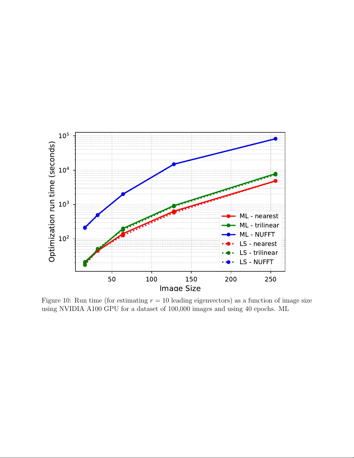
Leave a Comment