A Theoretical Framework for Modular Learning of Robust Generative Models

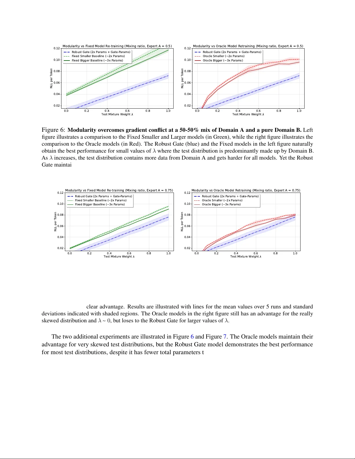
A Theoretical Frame work for Modular Learning of Rob ust Generati ve Models Corinna Cortes Google Research Ne w Y ork, NY 10011 corinna@google.com Mehryar Mohri Google Research & CIMS Ne w Y ork, NY 10011 mohri@google.com Y utao Zhong Google Research Ne w Y ork, NY 10011 yutaozhong@google.com Contents 1 Introduction 3 2 Related W ork 4 3 Setup & Problem F ormulation 5 4 Theoretical Analysis 7 4.1 Fixed Mixture . . . . . . . . . . . . . . . . . . . . . . . . . . . . . . . . . . . . . . . . . . . . . 7 4.2 Robust Existence . . . . . . . . . . . . . . . . . . . . . . . . . . . . . . . . . . . . . . . . . . . 7 4.3 Prior Kno wledge on Mixture W eights . . . . . . . . . . . . . . . . . . . . . . . . . . . . . . . 9 4.4 The Least-Fav orable Mixture . . . . . . . . . . . . . . . . . . . . . . . . . . . . . . . . . . . . 12 4.5 Comparison with Monolithic Baselines: Interference vs. Decoupling . . . . . . . . . . . . . . 12 4.5.1 The Monolithic Barrier: Di versity as Interference . . . . . . . . . . . . . . . . . . . . 12 4.5.2 The Modular Adv antage: Div ersity as Separability . . . . . . . . . . . . . . . . . . . 13 4.5.3 The Decoupling Hypothesis . . . . . . . . . . . . . . . . . . . . . . . . . . . . . . . . 14 4.5.4 Safety in Con ve x Settings . . . . . . . . . . . . . . . . . . . . . . . . . . . . . . . . . . 14 4.6 Generalization and Sample Ef ﬁciency . . . . . . . . . . . . . . . . . . . . . . . . . . . . . . . 15 5 Optimization Algorithms 18 5.1 Reformulation via Linearization . . . . . . . . . . . . . . . . . . . . . . . . . . . . . . . . . . 18 5.2 Scalable Primal-Dual Algorithm . . . . . . . . . . . . . . . . . . . . . . . . . . . . . . . . . . 20 5.3 Ef ﬁciency and Con ver gence . . . . . . . . . . . . . . . . . . . . . . . . . . . . . . . . . . . . . 20 5.4 Practical Implementation . . . . . . . . . . . . . . . . . . . . . . . . . . . . . . . . . . . . . . . 22 6 Sampling from the Rob ust Gated Model 23 6.1 Sampling-Importance-Resampling (SIR) . . . . . . . . . . . . . . . . . . . . . . . . . . . . . . 23 6.2 Exact Rejection Sampling . . . . . . . . . . . . . . . . . . . . . . . . . . . . . . . . . . . . . . 25 6.3 Baseline: Ef ﬁcient Sampling via Monolithic Distillation . . . . . . . . . . . . . . . . . . . . . 26 6.4 Inference Bottleneck . . . . . . . . . . . . . . . . . . . . . . . . . . . . . . . . . . . . . . . . . 26 1 7 Efﬁcient Inference: Structural Distillation 26 7.1 Monolithic vs. Structural Distillation . . . . . . . . . . . . . . . . . . . . . . . . . . . . . . . . 27 7.2 The Causal Router & Objective . . . . . . . . . . . . . . . . . . . . . . . . . . . . . . . . . . . 27 7.3 Cached-Logit Distillation Algorithm . . . . . . . . . . . . . . . . . . . . . . . . . . . . . . . . 28 7.4 Discussion . . . . . . . . . . . . . . . . . . . . . . . . . . . . . . . . . . . . . . . . . . . . . . . 28 8 Experiments 29 8.1 Empirical Comparison: Gate vs. Monolithic . . . . . . . . . . . . . . . . . . . . . . . . . . . . 29 8.2 Algorithm Stability and Con vergence . . . . . . . . . . . . . . . . . . . . . . . . . . . . . . . . 31 8.3 Experiments with Structural Distillation . . . . . . . . . . . . . . . . . . . . . . . . . . . . . . 32 8.4 Modularity for Real-W orld Data . . . . . . . . . . . . . . . . . . . . . . . . . . . . . . . . . . 32 8.5 Real-W orld Rob ustness to Distribution Shift . . . . . . . . . . . . . . . . . . . . . . . . . . . . 33 9 Conclusion 34 A Fixed-Mixture Optimal Solution: Characterization 39 B Capacity Lower Bound 40 C Discussion: Tightness vs. Inter pretability of the Bound 41 D Scalable Implementation and Inference 42 D.1 Architecture Parameterization . . . . . . . . . . . . . . . . . . . . . . . . . . . . . . . . . . . . 42 D.2 The Stochastic Primal-Dual Algorithm . . . . . . . . . . . . . . . . . . . . . . . . . . . . . . . 42 D.3 Practical Implementation Details . . . . . . . . . . . . . . . . . . . . . . . . . . . . . . . . . . 44 E Theoretical Analysis of Structured Distillation 45 2 Abstract T raining large-scale generati ve models is resource-intensiv e and relies heavily on heuristic dataset weighting. W e address two fundamental questions: Can we train Large Language Models (LLMs) modularly—combining small, domain-speciﬁc experts to match monolithic performance—and can we do so robustly for any data mixture, eliminating heuristic tuning? W e present a theoretical frame work for modular generative modeling where a set of pre-trained e xperts are combined via a gating mechanism. W e deﬁne the space of normalized gating functions, G 1 , and formulate the problem as a minimax game to ﬁnd a single robust g ate that minimizes div ergence to the worst-case data mixture. W e prove the e xistence of such a robust gate using Kakutani’ s ﬁxed-point theorem and show that modularity acts as a strong regularizer , with generalization bounds scaling with the lightweight gate’ s complexity . Furthermore, we prov e that this modular approach can theoretically outperform models retrained on aggregate data, with the gap characterized by the Jensen-Shannon Div ergence. Finally , we introduce a scalable Stochastic Primal-Dual algorithm and a Structural Distillation method for ef ﬁcient inference. Empirical results on synthetic and real-world datasets conﬁrm that our modular architecture effecti vely mitigates gradient conﬂict and can robustly outperform monolithic baselines. 1 Intr oduction T raining large-scale generati ve models, such as Lar ge Language Models (LLMs), is notoriously expensi ve and often impractical to repeat for e very new dataset [ Brown et al. , 2020 , Hoffmann et al. , 2022 ]. The computational cost and en vironmental footprint of these dense models hav e raised signiﬁcant sustainability concerns [ Strubell et al. , 2019 , Schwartz et al. , 2020 ]. This monolithic paradigm faces two critical challenges. First, sustainability and adaptability: can we train LLMs modularly , learning small, accurate models on indi vidual domains (e.g., math, coding) and combining them to match a giant model? If so, training becomes dramatically cheaper and greener; updates require training only a new module and the lightweight combiner , av oiding catastrophic forgetting [ Kirkpatrick et al. , 2017 , Parisi et al. , 2019 ] and enabling the efﬁcient reuse of pretrained e xperts [ Pfeiffer et al. , 2023 ]. In future, pri vac y regulations could also restrict access to data domains, smaller models trained by the data owners could constitute the only viable path to data access. Second, r ob ustness: standard training relies on heuristic importance weights across datasets [ Gao et al. , 2020 , T ouvron et al. , 2023 ], or static optimization targets [ Xie et al. , 2023 ], often failing when test distributions dif fer from training assumptions [ K oh et al. , 2021 ]. Can we b uild a modular LLM that is accurate for any mixture of datasets, eliminating heuristic weighting entirely? W e provide an afﬁrmati ve answer to both questions, offering the ﬁrst rigorous game-theoretic frame- work for robust modularity . Unlike heuristic approaches like simple parameter averaging (Model Soups) [ W ortsman et al. , 2022 ], task arithmetic [ Ilharco et al. , 2022 ], or standard Mixture of Experts which rely on auxiliary load-balancing losses [ Shazeer et al. , 2017 , Fedus et al. , 2022 ], we seek a single system that is robust to any arbitrary mixture of the underlying source distributions. W e propose a gated solution , π g ( x ) = ∑ k g ( x, k )  π k ( x ) , where an adaptiv e gate dynamically reweights frozen e xperts. Our goal is to ﬁnd a robust gate g ∗ that minimizes the div ergence to the worst-case data mixture, akin to Distributionally Rob ust Optimization (DR O) [ Sagaw a et al. , 2020 ]. Contributions. Our main contributions are: 1. Theor etical F rame work: W e deﬁne the normalized gate space G 1 and formulate robustness as a minimax game. W e prove the existence of a robust gate using Kakutani’ s ﬁxed-point theorem, establishing a stable upper bound on the worst-case risk (Theorem 3 ). 2. Generalization Analysis: W e deriv e bounds showing that sample complexity scales with the lightweight gate complexity and the expert coincidence norm C Π , rather than the massiv e expert parameters (Section 4.6 ). 3 3. Comparison with Retr aining: W e prov e an information-theoretic bound sho wing our modular approach can outperform monolithic retraining, with the performance gap characterized by the Jensen-Shannon Di vergence (Theorem 6 ). 4. Scalable Algorithm & Infer ence: W e introduce a Stochastic Primal-Dual algorithm for the constrained game and a Structur al Distillation method to map the non-causal gate to a causal router for efﬁcient autoregressi ve inference. 5. Empirical V alidation: W e demonstrate on synthetic benchmarks and real-w orld datasets (W ikipedia, Code, FineW eb) that our approach mitigates gradient conﬂict [ Y u et al. , 2020 ], outperforming baselines in high-interference regimes. Organization. Section 3 formalizes the problem. Section 4 presents existence proofs and comparisons. Section 5 details the optimization algorithm. Sections 6 and 7 addresses inference and distillation. Section 8 presents empirical results. 2 Related W ork Our proposed framew ork for robust modularity intersects with sev eral active areas of research, including model composition, theoretical routing, and the emerging economics of modular AI ecosystems. Robustness and Multiple-Source Adaptation. Our approach is rooted in the theory of multiple-source domain adaptation (MSA) [ Mansour et al. , 2008 , 2009 , Hof fman et al. , 2018 , Mohri et al. , 2021 , Hoffman et al. , 2022 , Cortes et al. , 2021 ], which seeks to learn predictors robust to mixtures of source domains. Recently , Dann et al. [ 2025 ] applied similar minimax principles to the problem of model routing. Their work addresses value-based routing, where the goal is to maximize a scalar reward (linear re gret). Our work can be vie wed as the generati ve counterpart to this line of research. By moving from linear rewards to the standard KL div ergence objecti ve which is needed for tackling generative modeling, we face a fundamentally dif ferent mathematical challenge: the resulting optimization problem is conv ex b ut non-linear , and crucially , requires enforcing a global normalization constraint ( Z g = 1 ) on the mixture model. This necessitates the constrained minimax analysis dev eloped in this paper , distinguishing our contribution from the unconstrained or locally-constrained optimization found in value-based routing or standard MSA. Our problem formulation also shares historical roots with the Meta-Pi network [ Hampshire II and W aibel , 1992 ], which combined expert outputs via a gating mechanism. Howe ver , their primary goal was rob ustness for the average dataset, whereas we target the worst-case mixture. Furthermore, while they demonstrated source-independence empirically , we provide rigorous existence and con vergence guarantees. Mixtures, Merging, and Composition. The concept of combining models has a rich history . Mixture of Experts (MoE) [ Jacobs et al. , 1991 , Fedus et a l. , 2022 ] trains a routing mechanism jointly with specialized sub-networks. In contrast, our framework operates on fr ozen, pr e-trained experts, decoupling the routing learning from the generativ e training. Another approach is Model Mer ging or Model Soups [ W ortsman et al. , 2022 ], which av erages weights to ﬁnd a single high-performing static model. Our approach differs by maintaining the experts as discrete entities and using an input-dependent gate g ( x, ⋅ ) to adapt to distribution shifts dynamically . Recent work explores deeper architectural integration. For example, Bansal et al. [ 2024 ] introduce Composition to Augment Language Models (CALM) , which le verages cross-attention to merge representations from a base LLM and specialized models, expanding capabilities without full retraining. Distinct from a symmetric modular vie w , this method designates one model as an anchor and the other as an augmenting 4 counterpart. It is also not clear how this construction scales beyond two models, as it may require a quadratic number of pairwise cross-attention connections. Complementary to this is model stitching [ Jiang and Li , 2024 ], where pre-trained blocks from disparate models, such as BER T and GPT , are integrated directly . Similarly , recent frameworks like StitchLLM [ Hu et al. , 2025 ] dynamically route requests across stitched blocks—for instance, feeding the lo wer layers of one model into the upper layers of another—to optimize the trade-of f between latency and accuracy . Crucially , neither approach provides theoretical analysis or guarantees for the resulting composed model. In contrast, our approach preserves experts as black boxes and of fers strong theoretical guarantees for a gating mechanism robust to worst-case distrib ution mixtures. Theoretical Routing and Learning to Defer . Our problem shares conceptual similarities with routing in learning to defer , where a learner chooses between predicting or deferring to experts. Foundational work by Cortes, DeSalvo, and Mohri [ 2016a , 2024 ], Mohri, Andor, Choi, Collins, Mao, and Zhong [ 2024 ] established the theory for learning with rejection in binary classiﬁcation. This line of work was signiﬁcantly expanded to multi-class settings and predictor-rejector frameworks by Mao et al. [ 2024a , b , 2023 , 2024c , e , d , 2025 ], DeSalvo et al. [ 2025 ], Mao [ 2025 ]. Our approach div erges from this literature in three key aspects. First, unlike standard routing which performs a hard selection of a single e xpert, our gated frame work induces a distribution over base models. Second, rather than optimizing for average-case performance, we address r ob ustness against adversarial distrib ution mixtures. Finally , while computational cost is a primary consid- eration in standard model routing, our current framework focuses purely on statistical performance guarantees. Modular Marketplaces and Ecosystems. Beyond functional integration, the rise of LLMs has spurred inter- est in the economic dynamics of modular systems. Bhawalkar et al. [ 2025 ] analyze “modular marketplaces” from a game-theoretic perspective, focusing on price equilibria where module owners act strategically to maximize proﬁt. Broader analyses of the AI ecosystem’ s ev olutionary dynamics [ Jacobides et al. , 2021 ] further highlight how the interplay between large upstream providers (e.g., cloud and foundation models) and specialized do wnstream modules is fundamentally reshaping industrial organization. Our work comple- ments these economic and ecosystem perspecti ves by pro viding the statistical equilibria—ensuring that the aggregated output of these traded modules remains rob ust regardless of ho w they are combined. 3 Setup & Pr oblem Formulation Let D k , k ∈ [ 1 , p ] , denote p datasets with empirical distributions  p k . W e assume access to pre-trained models  π k approximating each distribution with guarantees D KL (  p k ∥  π k ) ≤ ϵ k . W e consider gated solutions π g ( x ) = ∑ p k = 1 g ( x, k )  π k ( x ) , where g ( x, ⋅ ) ∈ ∆ is a gating function (see Figure 1 ). Our goal is to approximate any mixture  p λ = ∑ p k = 1 λ k  p k for λ ∈ ∆ . W e deﬁne the space of normalized gating functions G 1 as the subset of gates g ∈ ∏ x ∈ X 0 ∆ ([ 1 , p ]) , that is g ( x, k ) ≥ 0 and ∑ k g ( x, k ) = 1 for all x ∈ X 0 , satisfying the global normalization constraint: G 1 =  g ∶ Z g = ∑ x ∈ X 0 ∑ p k = 1 g ( x, k )  π k ( x ) = 1  , where X 0 =  k supp (  p k ) and is hence ﬁnite. For an y g ∈ G 1 , the resulting model π g is a v alid probability distribution. Lemma 1. The family G 1 is non-empty , compact, and conve x. Pr oof. G 1 is non-empty since for any λ ∈ ∆ ([ 1 , p ]) it contains the constant gate g λ ( x, k ) = λ k . G 1 is con ve x since G is con vex, as a product of simplices, and since the af ﬁne equality Z g = 1 is preserved by con ve x combinations. The base family G = ∏ x ∈ X 0 ∆ ([ 1 , p ]) is compact since each simplex ∆ ([ 1 , p ]) is compact and the product of compact sets (over the ﬁnite support X 0 , or e ven countable sets) is compact by T ychonof f ’ s theorem. The constraint function g ↦ Z g = ∑ x,k g ( x, k )  π k ( x ) is continuous since linear . The set G 1 = G ∩ { g ∶ Z g = 1 } is the intersection of a compact set, G , and a closed set, the lev el set { g ∶ Z g − 1 = 0 } 5 Input x Adaptive Gate g ( x, ⋅ ) Expert  π 1 ⋮ Expert  π p F r ozen / Pre-tr ained ∑ Robust Mixtur e π g ( x ) W eights g ( x, k ) Figure 1: Conceptual Architecture of the Modular Gated Solution. of a continuous function. Therefore, G 1 is closed. Since it is a closed subset of a compact set, it is also compact. Gi ven the setup, our objectiv e is to ﬁnd a single gating function g ∈ G 1 such that the resulting model π g is a high-quality approximation of an y data mixture  p λ . W e use the relati ve entrop y , D KL di vergence, as our measure of dissimilarity . This leads to two primary formulations. First, as a preliminary question, we can ask what performance is achiev able for a single, ﬁxed mixture λ . This corresponds to the standard con ve x optimization problem: min g ∈ G 1 D KL (  p λ ∥ π g ) . Finding a solution to this problem would pro vide an optimal gate for a known, static test distrib ution. Second, and more central to our goal of modularity and robustness, we ask for a single gate g ∗ that performs well against the worst-case mixture λ ∈ ∆ . This is a robust optimization problem that can be formulated as a minimax game: min g ∈ G 1 max λ ∈ ∆ ([ 1 ,p ]) D KL (  p λ ∥ π g ) . The solution g ∗ to this game would be a truly robust model, providing a uniform performance guarantee across the entire ambiguity set of possible data mixtures. Remark on Objective. Our use of the relative entrop y , rather than the cross-entropy loss, is essential. While minimizing KL is equiv alent to minimizing cross-entropy for a ﬁxed target distrib ution (since entropy is constant), this equiv alence breaks do wn in the robust setting. The entropy term H (  p λ ) v aries with the adversarial choice of λ . Consequently , minimizing the worst-case cross-entrop y max λ E  p λ [ − log π ] is not equi valent to minimizing the worst-case di vergence max λ D KL (  p λ  π ) . W e target the latter to ensure the model approximates the distribution  p λ itself, rather than merely cov ering its support. Our work aims to answer se veral fundamental theoretical and algorithmic questions arising from these formulations: 1. F ixed-mixtur e performance: For a ﬁxed mixture λ , does there exist a gated solution π g with small di vergence D KL (  p λ ∥ π g ) ? More speciﬁcally , how does this optimal error min g ∈ G 1 D KL (  p λ ∥ π g ) compare to the baseline errors ϵ k ? 2. Robust guarantee: Does there exist a r obust gated solution π g ∗ that achie ves small di ver gence for all λ ∈ ∆ ? This is a question of existence for the minimax problem min g max λ D KL (  p λ ∥ π g ) . 3. Construction and bounds: If such a robust solution exists, how can we construct it algorithmi- cally? What explicit, non-asymptotic guarantees can we provide for its worst-case performance, max λ D KL (  p λ ∥ π g ∗ ) , in terms of the indi vidual expert guarantees ϵ k ? 6 4. Comparison to ag gre gate training: For a ﬁxed mixture λ , ho w does the performance of our modular solution π g compare to that of a model  π λ trained from scratch on the aggregate data  p λ = ∑ p k = 1 λ k  p k ? Understanding this trade-of f is k ey to justifying the modular approach ov er the expensi ve, non-adaptive retraining baseline. In Section 4 , we will address these questions, starting with the existence and bounds for the ﬁxed and rob ust solutions. 4 Theor etical Analysis W e no w establish the existence of a rob ust gate and quantify its advantages o ver monolithic retraining. 4.1 Fixed Mixture First, we consider a simple non-adaptive baseline. If we ﬁx the mixture weights λ , a constant gate g λ ( x, k ) = λ k (which belongs to G 1 ) achie ves an av erage error bound. Proposition 2 (Fixed Mixture Guarantee) . F or any ﬁxed λ ∈ ∆ , the constant gate π λ = ∑ k λ k  π k satisﬁes D KL (  p λ ∥ π λ ) ≤ ∑ p k = 1 λ k ϵ k ≤ max k ϵ k . Pr oof. The result follows directly from the joint con vexity of the KL di ver gence: D KL (  p λ ∥ π λ ) = D KL  p  k = 1 λ k  p k ∥ p  k = 1 λ k  π k  ≤ p  k = 1 λ k D KL (  p k ∥  π k ) ≤ p  k = 1 λ k ϵ k . This completes the proof. This proposition guarantees average performance for a known mixture λ using a simple non-adaptive gate. (W e deri ve the e xact, though complex, optimal gate for a ﬁxed λ in Appendix A ). Ho wev er , we prove in Appendix B (Theorem 16 ) that any static weighting scheme is fundamentally limited by a capacity lower bound of log ( ∑ k e ϵ k ) , for disjoint domains. T o ov ercome this barrier and achiev e robustness to unknown λ , we require an input-dependent gate. 4.2 Robust Existence Here, we sho w the existence of a g ate model with a fa vorable guarantee for an y target mixture λ . W e will use the linearized game , which is deﬁned by the payoff  L ( λ, g ) = ∑ p k = 1 λ k D KL (  p k ∥ π g ) . Our analysis is presented in terms of the J ensen-Shannon Diver gence (JSD), which is a measure of di versity . For a mixture  p λ = ∑ k λ k  p k , JSD is deﬁned as the av erage KL div ergence from each source to the mixture: D λ JSD ({  p k }) = p  k = 1 λ k D KL (  p k ∥  p λ ) . JSD is non-negati ve and upper bounded by the Shannon entrop y H ( λ ) = − ∑ p k = 1 λ k log λ k . Theorem 3 (Rob ust Existence) . The linearized modular game admits a saddle point ( λ ∗ , g ∗ ) ∈ ∆ ([ 1 , p ]) × G 1 . F or any mixtur e λ ∈ ∆ , the r obust gate g ∗ satisﬁes for any λ ∈ ∆ ([ 1 , p ]) : D KL (  p λ ∥ π g ∗ ) ≤ log  p  k = 1 e ϵ k  − H λ ∗ σ ( K  X ) − D λ JSD ({  p k }) , wher e H λ ∗ σ ( K  X ) = ∑ p k = 1 λ ∗ k E x ∼  p k  − log σ k  π k ( x ) π σ ( x )  is the tar get-weighted conditional entr opy of the expert assignment under the r obust constant gate π σ = ∑ p k = 1 σ k  π k deﬁned by the softmax weights σ k = e ϵ k  ∑ p j = 1 e ϵ j . 7 Here, H λ ∗ σ ( K  X ) can be viewed as the overlap gain and D λ JSD as the diversity gain . Pr oof. The proof consists of casting the problem as a two-player , zero-sum game and showing the existence of a saddle point via Kakutani’ s Fixed Point Theorem. The original payoff function is L ( λ, g ) = D KL (  p λ ∥ π g ) . Since L is conv ex in λ , its maximizers lie strictly at the vertices. T o satisfy the con vexity requirement of Kakutani’ s theorem, we consider the linearized game with payof f:  L ( λ, g ) = p  k = 1 λ k D KL (  p k ∥ π g ) . W e deﬁne the best-response functions: Λ ∗ ( g ) = argmax λ ′ ∈ ∆ ([ 1 ,p ])  L ( λ ′ , g ) , G ∗ ( λ ) = argmin g ′ ∈ G 1  L ( λ, g ′ ) . W e show that the correspondence T ( λ, g ) = ( Λ ∗ ( g ) , G ∗ ( λ )) satisﬁes Kakutani’ s conditions: For G ∗ ( λ ) ,  L is con ve x in g (as a con ve x combination of con ve x KL terms), so the set of minimizers is con vex. For Λ ∗ ( g ) ,  L is linear in λ , so the set of maximizers is a con vex f ace of the simplex. Since  L is continuous and the domains are compact, Ber ge’ s Maximum Theorem implies Λ ∗ and G ∗ hav e closed graphs. Kakutani’ s ﬁxed-point theorem thus guarantees the e xistence of a ﬁxed point ( λ ∗ , g ∗ ) ∈ ( Λ ∗ ( g ∗ ) , G ∗ ( λ ∗ )) , which is a saddle point for  L . Bounding the V alue. W e now bound the worst-case risk of this optimal solution. By the saddle point property ,  L ( λ ∗ , g ∗ ) = max λ  L ( λ, g ∗ ) . W e use the fundamental identity relating the mixture risk L and the linearized risk  L : for any λ ∈ ∆ ([ 1 , p ]) , D KL (  p λ ∥ π g ∗ ) =  L ( λ, g ∗ ) − D λ JSD (  p 1 , . . . ,  p p ) ≤  L ( λ ∗ , g ∗ ) − D λ JSD (  p 1 , . . . ,  p p ) . (1) W e must bound  L ( λ ∗ , g ∗ ) . Since g ∗ is the minimizer of  L ( λ ∗ , ⋅ ) ov er G 1 , its loss is bounded by that of any speciﬁc witness gate. W e choose the Robust Constant Gate π σ deﬁned by the softmax weights σ k = e ϵ k  Z , where Z = ∑ e ϵ j (the solution of the proof of Theorem 16 ):  L ( λ ∗ , g ∗ ) ≤  L ( λ ∗ , π σ ) = p  k = 1 λ ∗ k D KL (  p k ∥ π σ ) . W e expand the component KL di ver gence D KL (  p k ∥ π σ ) . Since π σ ( x ) ≥ σ k  π k ( x ) : D KL (  p k ∥ π σ ) = E x ∼  p k  log  p k ( x ) π σ ( x )  = E x ∼  p k  log  p k ( x ) σ k  π k ( x ) + log σ k  π k ( x ) π σ ( x )  = D KL (  p k ∥  π k )      ϵ k − log σ k − E x ∼  p k  − log σ k  π k ( x ) π σ ( x )      H k ( K ∣ x ) . Substituting σ k = e ϵ k  Z , we hav e − log σ k = log Z − ϵ k . The ϵ k terms cancel: D KL (  p k ∥ π σ ) = log Z − H k ( K  x ) . A veraging over λ ∗ yields  L ( λ ∗ , g ∗ ) ≤ ∑ p k = 1 λ ∗ k ( log Z − H k ( K  x )) = log Z − H λ ∗ σ ( K  X ) . Sub- stituting this upper bound back into Eq. ( 1 ) completes the proof. While a numerically tighter bound is possible in the theorem statement, we leveraged the witness π σ in the proof to derive an explicit geometric form (see Appendix C for a detailed discussion on the trade-off between tightness and interpretability). The upper bound ( V ∗ ≤ LSE − Overlap − Div ersity ) re veals how the rob ust gate lev erages task geometry in three limiting regimes: 8 Case 1: The Specialization Limit (Disjoint Experts). Consider the case where task supports are mutually disjoint ( supp (  p k ) ∩ supp (  p j ) = ∅ ). • Geometry: The expert assignment is deterministic, so the ov erlap gain vanishes: H λ ∗ σ ( K  X ) = 0 . • Diversity: The diversity gain depends on the test mixture λ . For disjoint supports, it is equal to the entropy: D λ JSD = H ( λ ) . • Result: The bound becomes D KL (  p λ ∥ π g ∗ ) ≤ log ( ∑ e ϵ k ) − H ( λ ) . If the test mixture is difﬁcult (high entropy , e.g., balanced tasks), then H ( λ ) ≈ log p , canceling the capacity cost. This guarantees that the modular model incurs no capacity penalty precisely when the task is most complex. Case 2: The Redundancy Limit (Identical Experts). Consider the simpliﬁed case where all experts and targets are identical and ha ve equal error ϵ . • Geometry: T asks are indistinguishable ( D JSD = 0 ) and weights are uniform ( H ( σ ) = log p ). • Result: The capacity cost log ( pe ϵ ) = ϵ + log p is exactly refunded by the ov erlap gain ( log p ). V ∗ ≤ ( ϵ + log p ) − log p = ϵ. Thus, the modular system recov ers the performance of a single expert. Case 3: The Ensemble Mechanism (Exact Cancellation). W e now analyze the general mechanism of ov erlap for arbitrary errors. Consider the case where e xperts ov erlap fully (identical targets, D JSD = 0 ) b ut hav e different errors ϵ k . The ov erlap gain becomes the entropy of the robust weights H ( σ ) . W e recall that for the robust g ate, H ( σ ) = log Z − ∑ k σ k ϵ k . Substituting this into the bound: V ∗ ≤ log Z  Capacity Cost −  log Z − p  k = 1 σ k ϵ k       Overlap Gain H ( σ ) − 0  Div ersity (2) V ∗ ≤ p  k = 1 σ k ϵ k . (3) This deri v ation prov es that in the high-o verlap regime, the “Capacity Cost” (LogSumExp) is exactly cancelled by the ambiguity of the gate. The bound collapses to the weighted average err or of the experts. The modular system ef fectiv ely transforms into a static ensemble, pooling the experts to minimize risk. 4.3 Prior Knowledge on Mixtur e W eights In certain applications, we may have prior kno wledge suggesting that the mixture weights encountered at test time will be restricted to a con v ex subset Λ ⊂ ∆ ([ 1 , p ]) . This kno wledge can be lev eraged to deriv e a more specialized solution with signiﬁcantly stronger performance guarantees. The existence result from Theorem 3 extends directly to this scenario. By considering the linearized game restricted to the compact con vex set Λ , the con ve xity of the best-response sets is preserved, ensuring the existence of a saddle point via Kakutani’ s theorem. The value of this restricted g ame, V ∗ Λ , is guaranteed to be no worse than the original game value, V ∗ ∆ . The adversary ( λ -player) has a smaller set of strategies, which limits their ability to ﬁnd high-loss mixtures. This results in a lo wer worst-case loss for our solution: V ∗ Λ = min g ∈ G 1 max λ ∈ Λ L ( λ, g ) ≤ min g ∈ G 1 max λ ∈ ∆ ([ 1 ,p ]) L ( λ, g ) = V ∗ ∆ . 9 ∆ ([ 1 , p ]) (Full Simplex) Λ (Prior) λ ′ t (Unconstrained) λ t + 1 (Projected) Safety Margin Figure 2: Geometry of Prior Knowledge (Section 4.3 ). The outer triangle represents the full probability simple x ∆ . The green region Λ represents the subset of valid mixtures deﬁned by prior kno wledge. The algorithm projects the adversary’ s updates (red point) back onto Λ (blue point), tightening the w orst-case bound as per Theorem 5 . Intuiti vely , the gating function no longer needs to defend against unrealistic mixture weights outside of Λ . It can therefore specialize its performance for the kno wn set of likely scenarios. W e no w formalize the superiority of this specialized solution. Let g ∗ ∆ be the optimal robust gate found by solving the original problem over the full simplex ∆ , and let g ∗ Λ be the optimal gate found by solving the restricted problem ov er Λ (see Figure 2 ). Theorem 4 (Dominance of the Specialized Solution) . Let g ∗ ∆ be the optimal r obust gate over the full simplex ∆ ([ 1 , p ]) , and let g ∗ Λ be the optimal gate over the r estricted conve x set Λ ⊂ ∆ ([ 1 , p ]) . Then the worst-case performance of g ∗ Λ over Λ is at least as good as the performance of g ∗ ∆ over the same set: max λ ∈ Λ D KL (  p λ ∥ π g ∗ Λ ) ≤ max λ ∈ Λ D KL (  p λ ∥ π g ∗ ∆ ) . Pr oof. By deﬁnition of the restricted minimax solution g ∗ Λ , we hav e max λ ∈ Λ D KL (  p λ ∥ π g ∗ Λ ) = min g ∈ G 1 max λ ∈ Λ D KL (  p λ ∥ π g ) . Since g ∗ ∆ ∈ G 1 is a feasible gate, its performance must be greater than or equal to the minimum over all gates: min g ∈ G 1 max λ ∈ Λ D KL (  p λ ∥ π g ) ≤ max λ ∈ Λ D KL (  p λ ∥ π g ∗ ∆ ) . Combining the two statements gi ves the claimed inequality . T o make the beneﬁt more concrete, we can quantify the impro vement under a Lipschitz assumption. Theorem 5 (Quantitati ve Impro vement in Game V alue) . Assume that for any ﬁxed gate g ∈ G 1 , the mapping λ ↦ D KL (  p λ ∥ π g ) is L -Lipschitz with r espect to the ℓ 1 -norm:  D KL (  p λ ∥ π g ) − D KL (  p λ ′ ∥ π g ) ≤ L  λ − λ ′  1 , for all λ, λ ′ ∈ ∆ ([ 1 , p ]) . Let V ∗ ∆ = min g max λ ∈ ∆ D KL (  p λ ∥ π g ) be the minimax value o ver the full simplex, and let V ∗ Λ = min g max λ ∈ Λ D KL (  p λ ∥ π g ) be the value over the r estricted set. The impr ovement is bounded by: 0 ≤ V ∗ ∆ − V ∗ Λ ≤ L ⋅ d H ( Λ , ∆ ([ 1 , p ])) , wher e d H ( Λ , ∆ ([ 1 , p ])) = max λ ∈ ∆ ([ 1 ,p ]) min λ ′ ∈ Λ  λ − λ ′  1 is the Hausdorff distance between the sets. 10 Pr oof. For any ﬁx ed gate g , deﬁne the worst-case loss o ver a set S as F ( g , S ) = max λ ∈ S D KL (  p λ ∥ π g ) . Let λ ∗ ∈ ∆ ([ 1 , p ]) be a mixture that achie ves the maximum for the full simplex, i.e., D KL (  p λ ∗ ∥ π g ) = F ( g , ∆ ) . Let λ proj be the point in Λ closest to λ ∗ in the ℓ 1 -norm. By the deﬁnition of the Hausdorf f distance,  λ ∗ − λ proj  1 ≤ d H ( Λ , ∆ ) . Using the Lipschitz assumption: F ( g , ∆ ) − F ( g , Λ ) = D KL (  p λ ∗ ∥ π g ) − max λ ∈ Λ D KL (  p λ ∥ π g ) ≤ D KL (  p λ ∗ ∥ π g ) − D KL (  p λ proj ∥ π g ) (Since λ proj ∈ Λ ) ≤ L  λ ∗ − λ proj  1 ≤ L ⋅ d H ( Λ , ∆ ([ 1 , p ])) . This inequality holds for any gate g . Therefore: F ( g , ∆ ) ≤ F ( g , Λ ) + L ⋅ d H ( Λ , ∆ ) . T aking the minimum ov er g ∈ G 1 on both sides preserves the inequality: min g F ( g , ∆ ) ≤ min g F ( g , Λ ) + L ⋅ d H ( Λ , ∆ ) . Substituting the deﬁnitions V ∗ ∆ = min g F ( g , ∆ ) and V ∗ Λ = min g F ( g , Λ ) yields the upper bound. The lower bound V ∗ ∆ − V ∗ Λ ≥ 0 follo ws immediately because Λ ⊂ ∆ , so the maximum ov er Λ can nev er exceed the maximum ov er ∆ . Explicit Lipschitz Constant. In practice, if the support X 0 is ﬁnite and all probabilities are strictly positiv e, an explicit Lipschitz constant is L = max k ∈ [ 1 ,p ] max g ∈ G 1  x ∈ X 0  p k ( x ) log  p k ( x ) π g ( x )  . This constant bounds the maximum gradient of the loss with respect to the mixture weights λ . Crucially , it depends only on the extremal geometry of the e xperts and is independent of the mixture λ . Example. Consider a case with two e xperts: a high-quality model  π 1 ( ϵ 1 = 0 . 01 ) and a lo w-quality model  π 2 ( ϵ 2 = 0 . 5 ). The general solution g ∗ ∆ must be robust against the worst-case mixture λ = ( 0 , 1 ) , so its guaranteed performance V ∗ will be close to 0 . 5 . Howe ver , if we hav e prior knowledge that the second source will ne ver constitute more than 5% of the mixture (i.e., Λ = { λ  λ 2 ≤ 0 . 05 } ), the specialized solution g ∗ Λ can largely ignore this w orst-case scenario. Its guaranteed performance V ∗ Λ will be dramatically lower , focusing on mixtures dominated by the high-quality expert. Robustness to Mis-speciﬁcation. The specialized gate is naturally robust to small mis-speciﬁcations of the set Λ . The Lipschitz assumption allows us to bound the performance on a slightly expanded set Λ δ = { λ ∈ ∆ ([ 1 , p ])  ∃ λ ′ ∈ Λ ,  λ − λ ′  1 ≤ δ } . The performance of the gate g ∗ Λ degrades gracefully: max λ ∈ Λ δ L ( λ, g ∗ Λ ) ≤ V ∗ Λ + L δ. Algorithmic Adaptation. The optimization algorithm presented in Section 5 is easily modiﬁed to adapt to this scenario. The update step for the λ -player is simply augmented with a projection back onto the con v ex set Λ . First, we compute the standard intermediate update λ ′ t + 1 : λ ′ t + 1 ( k ) = λ t ( k ) exp ( η λ ℓ t ( k )) ∑ p j = 1 λ t ( j ) exp ( η λ ℓ t ( j )) . 11 Then, we project this distribution onto the restricted set Λ to obtain the new weights: λ t + 1 = P Λ ( λ ′ t + 1 ) = argmin q ∈ Λ D KL ( q ∥ λ ′ t + 1 ) . This ensures that the mixture weights always remain within the speciﬁed prior constraints. 4.4 The Least-F av orable Mixture Our minimax solution provides two crucial outputs: the robust gate g ∗ , and the least-fav orable mixture λ ∗ . It is important to note that λ ∗ corresponds to the saddle point of the linearized game  L ( λ, g ) = ∑ k λ k D KL (  p k ∥ π g ) , rather than the original con ve x-con vex payof f L . Consequently , λ ∗ identiﬁes the speciﬁc weighting of source domains that is maximally challenging for the modular ensemble in the linearized re gime. This insight is highly v aluable in practical scenarios where engineers must train a single, static model  π on the aggregated data  p λ (e.g., for reduced inference latency). Instead of resorting to heuristic choices for the mixture weights λ (such as uniform λ k = 1  p or weights based on dataset size), the optimal λ ∗ resulting from the no-regret algorithm provides a statistically principled alternati ve. By training a ne w model on the data mixture  p λ ∗ = ∑ k λ ∗ k  p k , the resulting model  π λ ∗ is optimized for the distribution where the underlying e xpert ensemble is most vulnerable (in terms of the upper bound  L ). This strategy ef fecti vely turns the worst-case scenario for the gated model into the training objective for the static model. 4.5 Comparison with Monolithic Baselines: Interference vs. Decoupling W e rigorously contrast the proposed Modular Robustness with standard Monolithic training by analyzing ho w each architecture interacts with the geometry of the task distributions. 4.5.1 The Monolithic Barrier: Diversity as Interfer ence Consider a monolithic model π mono trained to minimize the loss on the mixture  p λ = ∑ p k = 1 λ k  p k . The performance on individual tasks is go verned by the Jensen-Shannon Decomposition Identity . For any model π , the av erage task risk decomposes exactly into two terms: p  k = 1 λ k D KL (  p k ∥ π )      A verage T ask Risk = D KL (  p λ ∥ π )     Mixture Fit + D λ JSD (  p 1 , . . . ,  p p )     Interference . This equality rev eals a fundamental limitation. Even in the limit of inﬁnite capacity where the model ﬁts the global mixture perfectly ( D KL (  p λ ∥ π ) → 0 ), the av erage risk is strictly determined by the task diversity , measured by the Jensen-Shannon Di vergence ( D JSD ). W e formalize this in the follo wing theorem. Theorem 6 (The JSD Gap) . Let {  p k } p k = 1 be sour ce distributions and let ϵ k = min π ∈ Π D KL (  p k ∥ π ) be the best-in-class err or for each sour ce. Then, the risk of the optimal r etrained model  π λ satisﬁes: D KL (  p λ ∥  π λ ) ≥ p  k = 1 λ k ϵ k − D λ JSD (  p 1 , . . . ,  p p ) . 12 Pr oof. The proof relies on a fundamental identity for the KL div ergence of a mixture. For any model π and letting X = ∪ k supp (  p k ) , the follo wing equality holds: p  k = 1 λ k D KL (  p k ∥ π ) = p  k = 1 λ k  x ∈ X  p k ( x ) log  p k ( x ) π ( x ) = p  k = 1 λ k  x ∈ X  p k ( x )  log  p λ ( x ) π ( x ) + log  p k ( x )  p λ ( x )  =  x ∈ X  p  k = 1 λ k  p k ( x ) log  p λ ( x ) π ( x ) + p  k = 1 λ k   x ∈ X  p k ( x ) log  p k ( x )  p λ ( x )  = D KL (  p λ ∥ π ) + p  k = 1 λ k D KL (  p k ∥  p λ ) = D KL (  p λ ∥ π ) + D λ JSD (  p 1 , . . . ,  p p ) . Rearranging gi ves the identity: D KL (  p λ ∥ π ) = p  k = 1 λ k D KL (  p k ∥ π ) − D λ JSD (  p 1 , . . . ,  p p ) . This holds for an y π ∈ Π . W e select the optimal model for the mixture,  π λ , and use the f act that D KL (  p k ∥  π λ ) ≥ ϵ k for all k : D KL (  p λ ∥  π λ ) = p  k = 1 λ k D KL (  p k ∥  π λ ) − D λ JSD ({  p k }) ≥ p  k = 1 λ k ϵ k − D λ JSD ({  p k }) . This completes the proof. Since the av erage task risk is lower -bounded by D λ JSD , the worst-case domain loss max k D KL (  p k  π ) is also necessarily lower -bounded by this quantity . For a monolithic architecture, diversity manifests as Geometric Interference : the model is forced to collapse distinct distrib utions into a single centroid. Consequently , performance is dominated by the geometry of the problem rather than the difﬁculty of the tasks; e ven if tasks are tri vial to solve indi vidually ( ϵ k ≈ 0 ), the model fails if they are distinct ( D JSD ≫ 0 ). 4.5.2 The Modular Advantage: Diversity as Separability In contrast, the modular gating network effecti vely in v erts this relationship. The worst-case risk of the robust gate is bounded by (Theorem 3 ): Risk mod ≤ log   e ϵ k      Capacity Cost − D λ JSD (  p 1 , . . . ,  p p )     Separability Gain − H λ ∗ σ ( K  X )     Overlap . Here, the di vergence term appears with a negat ive sign. For the modular system, task div ersity acts as a Geometric Gain . In the high-diversity re gime (disjoint supports), the overlap v anishes ( H ≈ 0 ). Crucially , if the test mixture is diverse, the separability gain becomes maximal ( D λ JSD → H ( λ ) ). As sho wn in our geometric analysis (Section 4.2 ), this gain effecti vely cancels the entropy term in the capacity cost ( log ( ∑ e ϵ k ) ≈ ϵ max + H ( λ ) ). Consequently , for div erse mixtures, the bound simpliﬁes to the intrinsic error of the worst-case e xpert: D KL (  p λ ∥ π g ∗ ) ≤ max k ϵ k . 13 x Density 1 ( E x p e r t 1 ) 2 ( E x p e r t 2 ) The ar ea between the blue peaks and the r ed curve r epr esents the JSD Gap. G a t e d M i x t u r e g * ( L o w E n t r o p y ) R e t r a i n e d M o d e l Figure 3: V isualizing the JSD Gap. A gated model (blue) ﬁts distinct modes perfectly by routing inputs. A retrained model (red) suffers from capacity interference, forcing an entrop y increase proportional to the JSD. 4.5.3 The Decoupling Hypothesis This analysis identiﬁes a structural phase transition governed by data geometry . W e observe a Symmetric Diver gence Ef fect : the same quantity D λ JSD that acts as an interference penalty for the monolithic model acts as a separability bonus for the modular gate. In the High Diversity Re gime (large D λ JSD ), the Monolithic model hits an interference ﬂoor ( Risk ≥ D λ JSD ), forced to increase entropy to co ver disjoint supports (broad red curve in Figure 3 ). In contrast, the Modular model exploits this separation to cancel the capacity cost, maintaining the lo w-entropy precision of the original experts (sharp blue peaks). By effecti vely decoupling risk from geometry , the modular system is guaranteed to outperform the monolithic baseline on any mixture λ where the intrinsic task dif ﬁculty is lower than the geometric cost of mixing: max k ( ϵ k ) < D λ JSD (  p ) . 4.5.4 Safety in Con vex Settings Finally , one might ask: does modularity sacriﬁce performance when tasks are simple and compatible? W e prov e that in conv ex settings, the answer is no. W e assume Π is a linear model family (e.g., exponential families). Theorem 7 (Gated Model Coincides with Retraining) . Let Π be a linear model. F or a mixture  p λ , let π k = π ∗ (  p k ) denote the pr ojection of eac h component. Then, the best model trained on the mixtur e π ∗ (  p λ ) coincides exactly with the gated mixtur e of the best component models: π ∗ (  p λ ) = p  k = 1 λ k π k . Pr oof. By the Pythagorean equality for linear models applied to each component  p k and to an arbitrary model π ∈ Π [ Csiszár , 1975 , Csiszár and Matus , 2003 ], for an y p and any π ∈ Π , D KL ( p ∥ π ) = D KL ( p ∥ π ∗ ( p )) + D KL ( π ∗ ( p ) ∥ π ) . Denoting π k = π ∗ (  p k ) , we obtain for each k , D KL (  p k ∥ π ) = D KL (  p k ∥ π k ) + D KL ( π k ∥ π ) . Multiplying by λ k and summing up yields p  k = 1 λ k D KL (  p k ∥ π ) = p  k = 1 λ k D KL (  p k ∥ π k ) + p  k = 1 λ k D KL ( π k ∥ π ) . (4) 14 The functions π ↦ D KL (  p λ ∥ π ) and π ↦ ∑ k λ k D KL (  p k ∥ π ) dif fer by a constant independent of π . Speciﬁcally , p  k = 1 λ k D KL (  p k ∥ π ) − D KL (  p λ ∥ π ) = D λ JSD ( p 1 , . . . , p p ) . This constant difference implies they share the same unique minimizer over π ∈ Π . The minimizer of π ↦ ∑ k λ k D KL (  p k ∥ π ) ov er π ∈ Π is the same as the minimizer of π ↦ ∑ k λ k D KL ( π k ∥ π ) , which is equiv alent to minimizing − E π g [ log π ] , where π g = ∑ k λ k π k . Since Π is a linear model, the con vex combination π g lies in Π . Therefore, the unique minimizer of D KL ( π g ∥ π ) is π = π g . This establishes that π g is the minimizer of D KL (  p λ ∥ π ) , proving the ﬁrst claim: π g = π ∗ (  p λ ) . T o prov e the second claim, we set π = π g in ( 4 ): p  k = 1 λ k D KL (  p k ∥ π g ) = p  k = 1 λ k D KL (  p k ∥ π k ) + p  k = 1 λ k D KL ( π k ∥ π g ) . The second term on the right-hand side is, by deﬁnition, the Jensen-Shannon di ver gence of the projections, D λ JSD ( π 1 , . . . , π p ) . The left-hand side can be re written using the constant-shift identity we established earlier: p  k = 1 λ k D KL (  p k ∥ π g ) = D KL (  p λ ∥ π g ) + D λ JSD ( p 1 , . . . , p p ) . Substituting this back yields the claimed identity . This theorem ensures that modularity is a “safe” architectural prior: it loses nothing in con vex re gimes while providing strictly superior robustness guarantees in the presence of conﬂicting, non-con ve x distributions. The best model trained on the mixture  p λ coincides with the gated model obtained by mixing the best component models π k . In particular , retraining on the mixture does not improv e upon gating. 4.6 Generalization and Sample Efﬁciency The guarantees in Theorem 3 establish the existence of a robust gate on the empirical distributions  p k . A critical advantage of the modular frame work is that this robustness transfers ef ﬁciently to the true population distributions p k . The generalization gap of the gated model scales with the complexity of the lightweight gating network G 1 , rather than the massi ve complexity of the generati ve e xperts. T o formalize this, we present generalization bounds in terms of Rademacher complexity , using vector - v alued function classes. Assumption 8 (Bounded Expert Lik elihoods) . W e assume that the pr e-trained experts are bounded away fr om zer o on the support of the data distrib ution. That is, ther e exists a constant M > 0 such that for all x ∈ X 0 and all k ∈ [ 1 , p ] , the ne gative log-likelihood is bounded:  log  π k ( x ) ≤ M . This implies that for any valid pr obability mixtur e π g ( x ) , the pr obability is lower -bounded by e − M . In the conte xt of Large Language Models (LLMs) with ﬁnite vocab ulary sizes, this assumption is naturally satisﬁed. The standard Softmax function yields strictly positiv e probabilities for all tokens. Unless an expert explicitly masks a tok en to −∞ (assigning it zero probability), the log-likelihood remains ﬁnite. 15 V ector -V alued Rademacher Complexity . Let F be a class of functions mapping X 0 to R p and denote by f j the j -th component of f ∈ F . The empirical Rademacher comple xity associated to such a vector -valued class of functions is deﬁned by  R S ( F ) = 1 m E σ       sup f ∈ F m  i = 1 p  j = 1 σ i,j f j ( x i )       , with σ i,j ’ s independent Rademacher variables, that is independent uniformly distributed random v ariables taking values in { − 1 , + 1 } . Its expectation, R m ( F ) = E S   R S ( F )  , is the Rademacher comple xity of F . Note that for p = 1 , this coincides with the standard notion of Rademacher complexity for real-v alued functions. The vectorial e xtension is also called factor gr aph Rademacher comple xity in Cortes et al. [ 2016b ], in the context of structured prediction. W e will denote by p k the true distrib ution according to which the dataset D k is drawn (or a sample S k ), and will denote by R k m k ( G 1 ) the Rademacher complexity of G 1 for the distribution p k and a sample size m k . The Expert Coincidence Norm ( C Π ). Before stating the main bound, we introduce a data-dependent constant that captures the geometric relationship between the experts. Let  π ( x ) = (  π 1 ( x ) , . . . ,  π p ( x )) be the vector of e xpert likelihoods at input x . W e deﬁne the maximum e xpert coincidence norm C Π as: C Π = sup x ∈ X 0   π ( x ) 2 . This quantity naturally measures the di versity and conﬁdence of the ensemble. It satisﬁes C Π ∈ [ 0 , √ p ] . • Orthogonal Experts (Best Case): If the experts represent distinct tasks with disjoint supports (perfect modularity), then for any x , at most one expert assigns non-negligible probability . In this case,   π ( x ) 2 ≈  π k ( x ) ≤ 1 , so C Π ≤ 1 . • High Entropy (T ypical Case): For LLMs with large v ocabularies, indi vidual token probabilities are typically small (e.g., 10 − 5 ). Even if e xperts are correlated, the ℓ 2 norm of tiny probabilities remains small, often satisfying C Π ≪ 1 . • Redundant Experts (W orst Case): The upper bound C Π = √ p is reached only if all p experts are fully redundant and assign probability 1 to the same input simultaneously . Thus, C Π acts as a condition number for modularity: lo wer values indicate better separation between experts. Theorem 9 (Generalization Bound for Modular Gate Models) . Under Assumption 8 , for any δ > 0 , with pr obability at least 1 − δ over the dr aw of samples S k ∼ p m k k , the following inequality holds simultaneously for all g ∈ G 1 and λ ∈ ∆ : E x ∼ p λ [ − log π g ( x )] ≤ E x ∼  p λ [ − log π g ( x )] + p  k = 1 λ k        2 √ 2 C Π e M R k m k ( G 1 ) + M     log p δ 2 m k        . Pr oof. Let L G 1 = { x ↦ − log π g ( x )  g ∈ G 1 } be the loss class associated with the gating hypothesis space G 1 . For a ﬁx ed k ∈ [ p ] , by the standard Rademacher complexity generalization bounds (see e.g., Mohri et al. [ 2018 ]) for functions bounded by M , for any δ > 0 , with probability at least 1 − δ , the follo wing inequality holds for all g ∈ G 1 : E x ∼ p k [ − log π g ( x )] ≤ E x ∼  p k [ − log π g ( x )] + 2 R k m k ( L G 1 ) + M     log 1 δ 2 m k . 16 Thus, by the union bound, the following inequality holds simultaneously for all k ∈ [ p ] with probability at least 1 − δ : E x ∼ p k [ − log π g ( x )] ≤ E x ∼  p k [ − log π g ( x )] + 2 R k m k ( L G 1 ) + M     log p δ 2 m k . Multiplying each inequality by λ k and summing up yields that with probability at least 1 − δ , the follo wing holds for all g ∈ G 1 and λ ∈ ∆ : E x ∼ p λ [ − log π g ( x )] ≤ E x ∼  p λ [ − log π g ( x )] + p  k = 1 λ k        2 R k m k ( L G 1 ) + M     log p δ 2 m k        . W e now bound R k m k ( L G 1 ) in terms of R k m k ( G 1 ) , using the vector contraction established in [ Cortes, Kuznetso v , Mohri, and Y ang , 2016b ] (Lemma A.1) and [ Maurer , 2016 ]. This inequality holds for ℓ 2 -Lipschitz functions. W e vie w the gate function class G 1 as a vector -valued hypothesis class mapping inputs x ∈ X 0 to the simplex ∆ ⊂ R p . The loss function for a function g ∈ G 1 and a sample x i is deﬁned as − log ( π g ( x i )) = Ψ i ( u ) = − log ( u ⋅  π ( x i )) , where  π ( x i ) = (  π 1 ( x i ) , . . . ,  π p ( x i )) and u = ( g ( x i , 1 ) , . . . , g ( x i , p )) . Under Assumption 8 , for any ﬁxed sample x i , Ψ i is Lipschitz continuous with respect to the ℓ 2 norm. The gradient of Ψ i with respect to the vector u is: ∇ Ψ i ( u ) = − 1 u ⋅  π ( x i )  π ( x i ) . T o determine the Lipschitz constant, we examine the ℓ 2 norm of the gradient:  ∇ Ψ i ( u ) 2 =   π ( x i ) 2  u ⋅  π ( x i ) . First, consider the numerator . By the deﬁnition of the coincidence norm, we ha ve   π ( x i ) 2 ≤ C Π . Second, consider the denominator . By Assumption 8 , the mixture probability is lower -bounded by e − M . Thus:  ∇ Ψ i ( u ) 2 ≤ C Π e − M = C Π e M . The function is therefore C Π e M -Lipschitz with respect to the ℓ 2 norm. Thus, by the vector contraction lemma [ Cortes et al. , 2016b , Maurer , 2016 ], we hav e R k m k ( L G 1 ) ≤ √ 2 C Π e M R k m k ( G 1 ) . Plugging the right-hand side into the inequality pre viously proven completes the proof. Corollary 10 (Equal Sample Sizes) . In the common setting wher e all e xperts have equal sample sizes m k = m and the comple xity is uniform acr oss distributions (denoted R m ( G 1 ) ), the bound simpliﬁes. F or any δ > 0 , with pr obability at least 1 − δ , for all g ∈ G 1 and λ ∈ ∆ : E x ∼ p λ [ − log π g ( x )] ≤ E x ∼  p λ [ − log π g ( x )] + 2 √ 2 C Π e M R m ( G 1 ) + M  log p δ 2 m . 17 Comparison with Retrained Models. T o appreciate the theoretical adv antage of the modular approach, we compare Theorem 9 with the generalization error of a standard model retrained from scratch. Let Π be the hypothesis class of a full generativ e model (e.g., a Transformer with parameters Θ ). A model  π scratch trained on the aggregate data minimizes the empirical risk o ver Π . Standard generalization bounds for such models scale with the complexity of the full class: GenGap (  π scratch ) ≈ O ( R m ( Π )) . In contrast, our modular solution π g freezes the experts and only learns the gating function. Its generalization gap scales with the complexity of the g ate: GenGap ( π g ) ≈ O  C Π e M R m ( G 1 )  + O   M  log ( p  δ ) m   . Since G 1 is typically a lightweight network (e.g., a simple linear projection or small MLP with 10 3 - 10 5 parameters) while Π represents a Large Language Model (with 10 9 - 10 11 parameters), we ha ve R m ( G 1 ) ≪ R m ( Π ) . Furthermore, the impact of the number of experts p is mitigated by the orthogonality of the tasks. While a worst-case analysis suggests a √ p dependency (if C Π ≈ √ p ), in practical modular systems where e xperts are specialized (disjoint supports), we hav e C Π ≈ 1 . Consequently , the cost of robustness across p experts appears primarily as a negligible log arithmic term √ log p . This implies that the modular approach requires signiﬁcantly fe wer samples to learn a robust policy than retraining a monolithic model from scratch. 5 Optimization Algorithms The existence result (Theorem 3 ) guarantees a rob ust gate g ∗ but is non-constructi ve. T o compute this gate, we must solve the minimax game. Originally , we formulated the problem as min g ∈ G 1 max λ ∈ ∆ L ( λ, g ) with payof f L ( λ, g ) = D KL (  p λ ∥ π g ) . This payof f is con vex in both parameters (since  p λ is linear in λ and D KL is con ve x in ﬁrst argument), pre venting the direct application of standard descent-ascent guarantees. 5.1 Ref ormulation via Linearization T o deri ve a tractable algorithm, we reformulate the problem into an equi valent con vex-conca ve game. Since the function λ ↦ L ( λ, g ) is con ve x, its maximum ov er the simplex ∆ is alw ays achiev ed at a verte x. Thus, max λ L ( λ, g ) = max k D KL (  p k ∥ π g ) . This observ ation allows us to introduce a linearized payof f function:  L ( λ, g ) = p  k = 1 λ k D KL (  p k ∥ π g ) . This ne w game shares the same value as the original problem b ut is con vex-concave : linear in λ and con ve x in g . This structure allows us to apply standard no-regret dynamics. Speciﬁcally , if the λ -player uses Exponentiated Gradient and the g -player uses Online Gradient Descent, the system is guaranteed to conv erge (Algorithm 1 ). Theorem 11 (Con vergence of Dynamics) . Let  V = min g ∈ G 1 max λ ∈ ∆  L ( λ, g ) . If the pr ojection Π G 1 onto the normalized gate space can be computed, then with step sizes η λ ∝ 1  √ T and η g ∝ 1  √ T , the time-avera ged gate g T con ver ges to the optimal r obust solution: max λ ∈ ∆  L ( λ, g T ) −  V ≤ O    log p T   . 18 Algorithm 1 Robust Gate via No-Re gret Dynamics (EG + OGD) 1: Input: Models  π 1 , . . . ,  π p ; datasets D 1 , . . . , D p ; learning rates η λ , η g ; iterations T . 2: Initialize: λ 0 ( k ) = 1  p ; g 0 ( x, k ) = 1  p for all x, k . 3: for t = 0 to T − 1 do 4: (Compute Gains) For each e xpert k ∈ [ 1 , p ] , compute its gain for the λ -player: ℓ t ( k ) = D KL (  p k  π g t ) . 5: ( λ -update) Update mixture weights using Exponentiated Gradient on gains ℓ t : λ t + 1 ( k ) ∝ λ t ( k ) exp ( η λ ℓ t ( k )) and re-normalize. 6: ( g -update) Construct mixture  p λ t + 1 from new λ t + 1 . 7: Compute gradient v t ( x, k ) = − (  p λ t + 1 ( x ) π g t ( x ))  π k ( x ) for all ( x, k ) . 8: Compute intermediate update g ′ t + 1 = g t − η g v t . 9: Project onto constrained space: g t + 1 = Π G 1 ( g ′ t + 1 ) . 10: end for 11: Output: The time-averaged g ate g T = 1 T ∑ T t = 1 g t . Pr oof. The proof relies on the regret bounds for the players’ algorithms and the connection between average regret and the duality gap for time-averaged strategies in con vex-conca ve games. Let R λ T be the regret of the λ -player (using EG) and R g T be the regret of the g -player (using OGD ov er G 1 ). Standard bounds yield: R λ T ≤ M λ √ 2 T log p and R g T ≤ D G 1 M g √ T . Let λ T = 1 T ∑ T t = 1 λ t and g T = 1 T ∑ T t = 1 g t . By the properties of con ve x-concav e games, the duality gap of the time-av eraged strategies is bounded by the sum of average regrets: max λ ∈ ∆  L ( λ, g T ) − min g ∈ G 1  L ( λ T , g ) ≤ R λ T + R g T T . The value of the game is  V = min g max λ  L ( λ, g ) . By weak duality , we know for any λ T , min g ∈ G 1  L ( λ T , g ) ≤  V . Therefore, we can bound the suboptimality of g T : max λ ∈ ∆  L ( λ, g T ) −  V ≤ max λ ∈ ∆  L ( λ, g T ) − min g ∈ G 1  L ( λ T , g ) ≤ R λ T + R g T T ≤ M λ √ 2 T log p + D G 1 M g √ T T = D G 1 M g √ T + M λ √ 2 log p √ T . This prov es con ver gence of the time-averaged strate gy g T to the v alue of the game  V . As established in the reformulation,  V is the v alue of the original problem, and thus g T is a near-optimal rob ust gate. This theorem provides a solid theoretical foundation: if we could enforce the constraints exactly , we would prov ably ﬁnd the robust gate. Howe ver , the projection Π G 1 is computationally intractable for large sequence models because the global normalization constraint Z g = ∑ x ∈ X 0 π g ( x ) = 1 couples the updates across all inputs x in the support. The analysis extends to the case where a subset Λ ⊆ ∆ ([ 1 , p ]) is used (Section 4.3 ). Theorem 12 (Algorithmic Con ver gence on Λ ) . Let  V Λ = min g ∈ G 1 max λ ∈ Λ  L ( λ, g ) be the value of the r estricted con vex-concave game, wher e  L ( λ, g ) = ∑ k λ k D KL (  p k ∥ π g ) . Let g T be the time-averaged gate obtained by running the no-r e gr et algorithm (Algorithm 1 , modiﬁed with λ -updates pr ojected onto Λ ). Assume the gains and gradients ar e bounded. Then, the algorithm admits the following con verg ence guarantee: E  max λ ∈ Λ  L ( λ, g T ) −  V Λ ≤ O    log p T   . 19 Pr oof. The proof is a direct extension of Theorem 11 . The game remains con v ex-concav e. The g -player’ s algorithm and regret bound are unchanged. The λ -player no w runs a projected online mirror descent (OMD) algorithm, speciﬁcally , Exponentiated Gradient with a projection. The regret of this algorithm is still bounded relati ve to the best ﬁxed strategy in Λ ⊆ ∆ ([ 1 , p ]) . Since the OMD algorithm uses the negati ve entropy regularizer (which leads to EG), the regret bound remains R λ T ≤ O ( √ T log p ) . The standard analysis bounding the duality gap by the av erage regret, 1 T ( R λ T + R g T ) , applies directly , yielding the O (  log p  T ) con ver gence rate. 5.2 Scalable Primal-Dual Algorithm T o scale to lar ge generativ e models, we parameterize the gate g θ (e.g., as a T ransformer Encoder) and enforce the global constraint via Lagrangian relaxation. W e introduce a dual variable µ ∈ R corresponding to the equality constraint Z g = 1 , transforming the problem into a 3-player primal-dual game : min θ max λ ∈ ∆ ,µ ∈ R L ( θ , λ, µ ) = p  k = 1 λ k L NLL ( k , θ )     Robust NLL + µ ( Z g θ − 1 )      Penalty . The system simulates dynamics between three players: 1. λ -player (Adversary): Maximizes the mixture dif ﬁculty using Exponentiated Gradient. This ef fectiv ely upweights experts where the gate is currently underperforming. 2. µ -player (Constr aint): Performs Dual Ascent to enforce global normalization. If the total mass Z g θ > 1 , µ increases, penalizing the gate; if Z g θ < 1 , µ decreases. 3. g -player (Gate): Updates parameters θ to minimize the Lagrangian via AdamW . W e solve this using stochastic estimates, see Algorithm 2 and a detailed description in Algorithm 6 (Ap- pendix D.2 ). Algorithm 2 Stochastic Primal-Dual T raining Loop 1: for iteration t = 1 to T do 2: Data Sampling: Sample batch B = ∪ k B k from experts. 3: Forward P ass: Compute logits g θ ( x ) and expert log-probs for x ∈ B . 4: Constraint Est.: Estimate  Z ≈ 1 ∣ B ∣ ∑ x ∈ B π g ( x ) q ( x ) via Importance Sampling, where q ( x ) = 1 p ∑  π k ( x ) is the uniform mixture proposal. 5: λ -Step (Adversary): Update mixture weights: 6: λ k ← λ k ⋅ exp ( η λ ⋅ ℓ k ) { ℓ k : loss on domain k } 7: µ -Step (Constraint): µ ← µ + η µ (  Z − 1 ) . 8: g -Step (Gate): Update θ to minimize L via AdamW . 9: end for 5.3 Efﬁciency and Con ver gence The Primal-Dual formulation fundamentally alters the computational proﬁle of the problem, making it feasible for LLMs. Optimization Complexity . The standard projection onto G 1 requires solving a constrained quadratic program ov er the entire support X 0 , which is impossible for sequence models. In contrast, our constraint is enforced 20 via a scalar update µ , costing O ( 1 ) per parameter . The partition function Z is estimated efﬁciently using the training batch itself as the importance sampling proposal, av oiding auxiliary data generation. Theoretical Guarantee. Crucially , replacing the hard projection with a Lagrangian penalty does not sacriﬁce the con ver gence guarantee. The Primal-Dual dynamics approximate the solution to the constrained game with the same asymptotic rate. Theorem 13 (Conv ergence of Primal-Dual Dynamics) . Consider the Lagrangian payoff L ( g , λ, µ ) =  L ( λ, g ) + µ ( Z g − 1 ) . Under the same con vexity assumptions as Theor em 11 , the time-averag ed iterates ( g T , λ T ) gener ated by Algorithm 2 conver ge to the optimal r obust solution with err or O ( 1  √ T ) , and the constraint violation decays at r ate O ( 1  √ T ) : max λ  L ( λ, g T ) −  V ≤ O  1 √ T  and  Z g T − 1  ≤ O  1 √ T  . Pr oof. The proof relies on viewing the optimization of the Lagrangian L ( θ , λ, µ ) as a zero-sum game between a primal player (controlling g θ ) and a dual player (controlling λ, µ ). W e analyze the con ver gence using the frame work of online con ve x optimization (OCO) and regret bounds. 1. The Lagrangian and Duality Gap. Recall the Lagrangian of the reformulated game: L ( g , λ, µ ) =  L ( λ, g ) + µ ( Z g − 1 ) = p  k = 1 λ k D KL (  p k ∥ π g ) + µ    x ∈ X 0 π g ( x ) − 1   . This function is con vex in the primal v ariable g (as established in Lemma 1 and Section 5.1 ) and linear (concav e) in the dual variables λ, µ . Let w = ( λ, µ ) denote the combined dual variables. The algorithm generates a sequence of iterates ( g t , w t ) T t = 1 . W e deﬁne the duality gap for the time-av eraged iterates ( g T , w T ) as: Gap ( g T , w T ) = max w ∈ W L ( g T , w ) − min g ∈ G 1 L ( g , w T ) , where W is a compact subset of the dual space containing the optimal dual solution w ∗ . 2. Regret Decomposition. A standard result in game dynamics (e.g., Freund and Schapire , 1999 , Cesa- Bianchi and Lugosi , 2006 ) states that the duality gap is bounded by the sum of the av erage regrets of the players. Let R g T be the regret of the g -player minimizing L ( ⋅ , w t ) and R w T be the combined regret of the dual players maximizing L ( g t , ⋅ ) . Gap ( g T , w T ) ≤ R g T + R w T T . 3. Bounding the Regrets. W e analyze the regret for each player based on their speciﬁc update rules in Algorithm 2 : • The λ -player (Simple x): Updates λ using Exponentiated Gradient (EG). F or linear losses with gradients bounded by M λ , the regret of EG o ver the simplex is bounded by: R λ T ≤ M λ  2 T log p. • The µ -player (Scalar Constraint): Updates µ using Gradient Ascent (Dual Ascent). Assuming the constraint violation (gradient w .r .t µ ) is bounded by M µ = max g  Z g − 1  and the optimal µ ∗ lies in a bounded range [ − D µ , D µ ] , standard Gradient Ascent bounds gi ve: R µ T ≤ D µ M µ √ T . 21 • The g -player (Gate P arameters): Updates g (via θ ) using AdamW (a v ariant of Online Mirror Descent). Under the con ve xity assumption of  L w .r .t g and bounded gradients M g , the regret is bounded by: R g T ≤ D G 1 M g √ T . 4. Con vergence Rate. Summing these terms, the total average re gret scales as: R total T T ≤ C √ T T = O  1 √ T  . Thus, the duality gap decays at a rate of O ( 1  √ T ) . 5. Recovering the Objectiv es. The con ver gence of the duality gap implies con ver gence of both the objecti ve v alue and the constraint satisfaction: • Rob ust Loss: max λ  L ( λ, g T ) −  V ≤ Gap ( g T , w T ) ≤ O ( 1  √ T ) . • Constraint V iolation: The Lagrangian term µ ( Z g − 1 ) implies that if the constraint is violated (  Z g T − 1  > ϵ ), the dual player µ would exploit this to maximize the gap. Therefore, the constraint violation is also bounded by the gap:  Z g T − 1  ≤ Gap ( g T , w T )  µ ∗  ≤ O  1 √ T  . This completes the proof that the Primal-Dual algorithm con ver ges to the optimal robust solution while asymptotically satisfying the normalization constraint. This theorem ensures that e ven without the expensiv e projection step, the algorithm pro vably reco vers the robust modular g ate. Gap between Theory and Practice. The con ver gence guarantees provided in Theorem 11 and Theorem 13 rely on the con vexity of the optimization problem with respect to the gate g . In our scalable implementation, the gate g θ is parameterized by a deep neural network, rendering the objecti ve non-con v ex with respect to θ . While strict no-regret guarantees do not apply to this non-con vex setting, we empirically observe that the Primal-Dual algorithm conv erges to effecti ve robust solutions, consistent with the success of similar game-theoretic optimization dynamics in deep learning (e.g., GANs or adversarial training). 5.4 Practical Implementation T ranslating the theoretical algorithm into a stable training loop requires addressing tw o speciﬁc numerical challenges: estimating the global partition function Z g and av oiding underﬂow . See Appendix D for a more detailed discussion. Estimating the Partition Function. Calculating the global sum Z g = ∑ x ∈ X 0 π g ( x ) exactly is intractable. W e rely on a Monte Carlo estimate using the current training batch B . Crucially , to av oid expensi ve auxiliary sampling, we use the training batch itself as the proposal distribution for Importance Sampling. The batch is constructed by sampling uniformly from the p source datasets, ef fectiv ely drawing x ∼ 1 p ∑ k  p k . Under the assumption that experts approximate their sources (  π k ≈  p k ), the empirical mixture closely matches the model mixture proposal q ( x ) = 1 p ∑ k  π k ( x ) . The estimator becomes:  Z = 1 ∣ B ∣ ∑ x ∈ B π g ( x ) q ( x ) . This allo ws us to reuse the logits computed during the forward pass, estimating the global constraint with zero additional inference cost. T o reduce v ariance in the µ -update, we track  Z using an Exponential Moving A verage (EMA). 22 T eacher Inference System A. Monolithic Distillation Non-Causal Gate g ∗ Frozen Experts {  π k } x Train via D robust (Next-token pred.) Causal Student π causal ( x ) (All knowledge baked in) Experts Discarded B. Structural T ransfer Non-Causal Gate g ∗ x Distill Routing W eights Only Causal Router γ ϕ ( x < t ) Original Frozen Experts {  π k } W eighted Mixing Figure 4: Efﬁ ciency Strategies. (A) Monolithic Distillation trains a single large model to mimic the ensemble, discarding the original experts. (B) Structural Distillation trains a lightweight Causal Router to mimic only the gating decisions ( g ∗ ), preserving the original experts. This maintains modularity: upgrading an expert in (B) improv es the system immediately . Log-Space Stability . The mixture probability π g ( x ) = ∑ k g ( x, k )  π k ( x ) in volv es summing probabili- ties that may be extremely small (e.g., 10 − 100 for long sequences). Direct computation leads to catas- trophic underﬂo w . W e strictly perform all operations in log-space using the LogSumExp trick: log π g ( x ) = LogSumExp k ( log g ( x, k ) + log  π k ( x )) . Quadratic Penalty . An alternativ e to the Lagrangian method is to relax the hard constraint into a soft quadratic penalty , min g max λ L ′ ( λ, g ) + β ( Z g − 1 ) 2 . This eliminates the need for the µ -player , reducing the problem to a standard regularized minimax optimization. Ho wev er , it only guarantees approximate normalization. W e ﬁnd the Primal-Dual approach superior as it dynamically adjusts the penalty strength µ to satisfy the constraint exactly in the limit. 6 Sampling fr om the Robust Gated Model The optimization procedure yields a robust gate g ∗ ∈ G 1 that guarantees the mixture model π g ∗ ( x ) = ∑ k g ∗ ( x, k )  π k ( x ) is globally normalized. Ho wev er , sampling from this model presents a unique challenge: the optimal gate g ∗ ( x, ⋅ ) is non-causal . It determines the mixture weights based on the com plete sequence x , meaning the probability of the ﬁrst token theoretically depends on the last. This breaks the standard autoregressi ve property required for ef ﬁcient token-by-tok en generation. T o sample from π g ∗ , we must rely on methods that treat the model as an unnormalized density or a re-weighted approximation. W e explore two Monte Carlo strategies. 6.1 Sampling-Importance-Resampling (SIR) The primary goal in this section is to draw sequence samples from the robust, gated model π g ∗ . While our optimization successfully ﬁnds a gate g ∗ that ensures the distribution π g ∗ ( x ) = ∑ k g ∗ ( x, k ) ˆ π k ( x ) is globally normalized, the resulting model presents a unique challenge for standard LLM inference. Standard LLMs generate text autore gressiv ely , predicting the next token based solely on past tokens. Ho wev er , our optimal gate g ∗ ( x, ⋅ ) is non-causal: it determines the mixture weights based on the complete sequence x , meaning the probability of the ﬁrst tok en theoretically depends on the last. Since we cannot generate tokens one by one if the routing logic depends on the ﬁnished sentence, we must resort to approximation methods like Sampling-Importance-Resampling (SIR) that generate complete candidates ﬁrst and score them later . 23 Algorithm 3 Sampling via Sampling-Importance-Resampling (SIR) 1: Input: Robust gate g ∗ ∈ G 1 , expert models {  π k } p k = 1 , number of candidates N . 2: Initialize: Empty lists C ← [] (candidates) and W ← [] (weights). 3: {Step 1: Generate N candidates from the proposal q ( x ) .} 4: for i = 1 to N do 5: Sample expert k ∼ Uniform ({ 1 , . . . , p }) . 6: Sample sequence x ( i ) ∼  π k ( x ) (autoregressi vely). 7: Append x ( i ) to C . 8: end for 9: {Step 2: Compute importance weights.} 10: for i = 1 to N do 11: x ← C [ i ] . 12: {This step requires ev aluating g ∗ and all p experts on x .} 13: Compute π g ∗ ( x ) = ∑ p k = 1 g ∗ ( x, k )  π k ( x ) . 14: Compute q ( x ) = 1 p ∑ p k = 1  π k ( x ) . 15: w i ← π g ∗ ( x ) q ( x ) if q ( x ) > 0 else ( 0 if π g ∗ ( x ) = 0 , ∞ otherwise). {Handle q ( x ) = 0 case.} 16: Append w i to W . 17: end for 18: {Step 3: Resample one candidate based on weights.} 19: Filter out candidates with non-ﬁnite weights. Let indices be I f inite . 20: Calculate total weight W sum = ∑ j ∈ I f inite W [ j ] . 21: if W sum = 0 or not is ﬁnite( W sum ) then {If all weights are zero or inﬁnite} 22: Sample i ∗ uniformly from { 1 , . . . , N } . {Fallback: uniform choice or error} 23: else 24: Deﬁne normalized probabilities P i = W [ i ] W sum for i ∈ I f inite (0 otherwise). 25: Sample an index i ∗ ∼ Categorical ({ P i } N i = 1 ) . 26: end if 27: x ∗ ← C [ i ∗ ] . 28: Return: The ﬁnal sample x ∗ . The SIR algorithm deri ves its name from its three distinct stages, each addressing a speciﬁc part of this non-causal hurdle: 1. Sampling: Since we cannot sample directly from the target π g ∗ , we ﬁrst generate a set of N candidate sequences from a pr oposal distribution q ( x ) that is easy to sample from. W e deﬁne this proposal as the uniform mixture of our e xperts, q ( x ) = 1 p ∑ ˆ π k ( x ) . This allo ws us to use standard autoregressi ve generation: we simply pick an expert at random and ha ve it generate a full sequence. 2. Importance: W e ackno wledge that these candidates were drawn from the wr ong distribution ( q instead of π g ∗ ). T o correct for this, we assign an importance weight w ( x ) to each candidate, calculated as the likelihood ratio w ( x ) = π g ∗ ( x ) q ( x ) = ∑ p k = 1 g ∗ ( x,k )  π k ( x ) 1 p ∑ p k = 1  π k ( x ) . This step is computationally e xpensiv e but feasible because we are e v aluating completed sequences; we can pass the full candidate x to the non-causal gate g ∗ to compute its true probability under the robust model. 3. Resampling: Finally , to obtain samples that approximate the robust target distrib ution, we resample from our pool of candidates. A candidate is selected with probability proportional to its importance weight, ensuring that sequences with high probability under the robust model π g ∗ are more likely to be chosen as the ﬁnal output. The pseudocode of the SIR algorithm is shown in Algorithm 3 . The inclusion of the fallback mechanism (Line 19) is a safe guard against numerical instability (underﬂo w), rather than a theoretical necessity . Struc- 24 turally , the absolute continuity assumption required for SIR consistency is strictly satisﬁed: since both the target π g ∗ and the proposal q are mixtures of the same set of e xperts {  π k } , the support of the target is con- tained within the support of the proposal ( supp ( π g ∗ ) ⊆  k supp (  π k ) = supp ( q ) ). Therefore, the theoretical case where q ( x ) = 0 and π g ∗ ( x ) > 0 (leading to inﬁnite weights) is impossible. Biased uniform sampling is thus only triggered in rare cases of ﬂoating-point underﬂo w . The computational cost is concentrated in the weight calculation (Line 11). Evaluating the tar get density π g ∗ ( x ) requires a full forward pass of the gate and all p experts for each of the N candidate sequences. Thus, the inference cost scales as O ( N p ) , moti vating the need for the ef ﬁcient distillation methods proposed in Section 6.3 . 6.2 Exact Rejection Sampling While SIR provides asymptotic guarantees, Rejection Sampling offers a method to obtain exact samples from the robust distrib ution π g ∗ , provided we can strictly bound the ratio between the tar get and the proposal. Recall that Rejection Sampling is a fundamental Monte-Carlo technique used to generate observ ations from a complex target distribution π ( x ) using a simpler , tractable proposal distribution q ( x ) . The main idea is: if we can ﬁnd a constant M such that the scaled proposal M q ( x ) always envelopes t he target (i.e., π ( x ) ≤ M q ( x ) for all x ), we can sample from q ( x ) and stochastically accept points that fall under the curve of π ( x ) . Samples where M ⋅ q ( x ) is much larger than π ( x ) are rejected more frequently , effecti vely carving out the correct distribution from the proposal. In our frame work, we can again use the uniform mixture of experts as the proposal, q ( x ) = 1 p ∑ p k = 1  π k ( x ) . A crucial property of our normalized gate space G 1 allo ws us to deriv e the strictly required bound M . Since the gating weights g ∗ ( x, k ) are probabilities bounded by 1 , the robust model’ s likelihood is strictly bounded by the sum of the indi vidual experts: π g ∗ ( x ) = p  k = 1 g ∗ ( x, k )  π k ( x ) ≤ p  k = 1  π k ( x ) = p q ( x ) . This provides the strict en velope constant M = p . Algorithm 4 Exact Sampling via Rejection Sampling 1: Input: Robust gate g ∗ ∈ G 1 , expert models {  π k } p k = 1 . 2: Output: An exact sample x ∗ ∼ π g ∗ . 3: loop 4: Sample expert k ∼ Uniform ({ 1 , . . . , p }) . 5: Sample candidate x ∼  π k ( x ) . {Proposal x ∼ q ( x ) } 6: Compute acceptance probability: A ( x ) = π g ∗ ( x ) M q ( x ) = π g ∗ ( x ) p q ( x ) 7: Sample u ∼ Uniform ([ 0 , 1 ]) . 8: if u ≤ A ( x ) then 9: retur n x 10: end if 11: end loop The ef ﬁciency of Rejection Sampling is strictly determined by the constant M = p , which represents the ratio of the area under the en veloping proposal M q ( x ) to the area under the target π g ∗ ( x ) . Geometrically , the algorithm samples points uniformly under the en velope; the probability that such a point also falls under the target curv e is exactly 1  M . Consequently , the number of trials required to ﬁnd a successful sample follows a geometric distribution with an e xpected value of M = p . 25 This re veals a clear trade-of f: for a moderate number of e xperts (e.g., p ≤ 10 ), the computational waste of rejecting candidates is a reasonable price for obtaining unbiased, exact samples. Ho wev er , because the bound M = p gro ws linearly with the ensemble size, the acceptance rate 1  p drops rapidly . For large p (e.g., p = 100 ), one would discard approximately 99% of generated candidates, making the method prohibitiv e. In these high-dimensional regimes, SIR becomes the preferred alternati ve. 6.3 Baseline: Efﬁcient Sampling via Monolithic Distillation While the Rejection Sampling and SIR algorithms provide exact or asymptotically exact samples from the robust model π g ∗ ( x ) , their inference cost scales linearly with the number of experts ( O ( p ) or O ( N p ) per sample), which may be prohibitiv e for large-scale deployment. The bottleneck is the non-causal nature of the optimal gate g ∗ ( x, k ) , which depends on the complete sequence x , pre venting ef ﬁcient caching or standard token-by-token generation. T o achie ve ef ﬁcient, constant time with respect to p , autor e gr essive sampling , we can distill the robust kno wledge from the non-causal target model π g ∗ into a new causal student model π causal , in a way somewhat similar to [ Hinton et al. , 2015 ]. This student model is parameterized as a standard causal T ransformer with parameters θ , ensuring the factorization π causal ( x ) = ∏ T t = 1 π causal ( x t  x < t ) . W e train the student model by minimizing the Kullback-Leibler di vergence from the rob ust target π g ∗ to the student π causal ov er the space of sequences: min θ D KL ( π g ∗ ∥ π causal ) = min θ E x ∼ π g ∗  − T  t = 1 log π causal ( x t  x < t ) − H ( π g ∗ ) . In practice, this is equiv alent to maximizing the log-likelihood of the student model on a dataset of synthetic sequences generated from π g ∗ . The training procedure is as follo ws: 1. Generate Data: Use the exact Rejection Sampling method (Algorithm 4 ) or SIR (Algorithm 3 ) to generate a large dataset of rob ust sequences D robust = { x ( i ) } M i = 1 drawn from π g ∗ . 2. T rain Student: T rain the causal T ransformer π causal on D robust using standard cross-entropy loss (ne xt- token prediction). This distillation step transfers the robustness guarantees of the non-causal gate into the weights of the causal student. At inference time, the expensi ve ensemble π g ∗ is discarded, and samples are drawn ef ﬁciently from π causal using standard autoregressi ve decoding. 6.4 Inference Bottleneck While these methods preserve the theoretical rob ustness guarantees, their inference cost scales linearly with the number of experts p . Evaluating the acceptance probability or importance weight requires running a forward pass on all p experts for e very candidate sequence. For lar ge ensembles (e.g., p = 100 ), this cost is prohibiti ve for real applications, moti vating the need for distillation. 7 Efﬁcient Infer ence: Structural Distillation While the robust gate g ∗ guarantees optimal performance, its non-causal nature requires expensiv e sampling methods like SIR or Rejection Sampling (Section 6 ) during inference. With Structural Distillation , we recov er efﬁcient O ( 1 ) autoregressi ve generation while preserving the beneﬁts of modularity . 26 7.1 Monolithic vs. Structural Distillation Standard distillation would in volv e training a single large student model to mimic the input-output behavior of the ensemble π g ∗ (see Section 6.3 ). While efﬁcient at inference time, this Monolithic Distillation (Figure 4 (A)) discards the modular structure: if one expert is updated or a ne w domain is added, the entire student model must be retrained from scratch. In contrast, our Structural Distillation approach (Figure 4 (B)) preserves the pre-trained experts (see detailed analysis in Appendix E ). W e distill the robust, non-causal gate g ∗ into a lightweight Causal Router γ ϕ . The inference system remains a mixture of experts, but the routing decisions are no w made causally . 7.2 The Causal Router & Objective W e deﬁne the student model π γ as a causal mixture of the frozen experts, parameterized by a learnable router γ ϕ : π γ ( x ) = T  t = 1 π γ ( x t  x < t ) = T  t = 1 p  k = 1 γ ϕ ( x < t , k )  π k ( x t  x < t ) . Here, γ ϕ ( x < t , ⋅ ) ∈ ∆ is a distribution over experts predicted by a small causal network (e.g., a shallo w T ransformer) gi ven only the history . Our goal is to train ϕ to minimize the KL di ver gence from the rob ust teacher π g ∗ to the student π γ ov er the sequence space X : min ϕ J ( ϕ ) = D KL ( π g ∗ ∥ π γ ) = E x ∼ π g ∗  log π g ∗ ( x ) π γ ( x )  . Crucially , this global sequence-lev el objectiv e decomposes into a tractable token-le vel optimization. Proposition 14 (Decomposition of Structural Distillation) . Minimizing the sequence-level diverg ence D KL ( π g ∗ ∥ π γ ) is equivalent to maximizing the expected log-likelihood of the student model on trajec- tories sampled fr om the r ob ust teacher . Speciﬁcally , the gradient is: ∇ ϕ J ( ϕ ) = − E x ∼ π g ∗  T  t = 1 ∇ ϕ log  p  k = 1 γ ϕ ( x < t , k )  π k ( x t  x < t ) . Pr oof. W e expand the deﬁnition of the KL di ver gence: J ( ϕ ) = E x ∼ π g ∗ [ log π g ∗ ( x )] − E x ∼ π g ∗ [ log π γ ( x )] . The ﬁrst term is the ne gati ve entropy of the teacher distribution π g ∗ and is ﬁx ed. Thus, minimizing the KL di vergence is equiv alent to maximizing the second term. Unlike the teacher , the student model π γ is deﬁned to be causal and autoregressi ve. Therefore, its log-probability factors into a sum of conditional log-probabilities: log π γ ( x ) = T  t = 1 log π γ ( x t  x < t ) . Substituting this back into the expectation yields: max ϕ E x ∼ π g ∗  T  t = 1 log  p  k = 1 γ ϕ ( x < t , k )  π k ( x t  x < t ) . T aking the gradient gi ves the result. This result allows us to train the router using standard MLE on a dataset of “rob ust sequences" generated by the teacher (using Rejection Sampling). Furthermore, we prove in Theorem 18 (Appendix E ) that this objecti ve minimizes the Router Appr oximation Err or , with no irreducible structural mismatch. 27 7.3 Cached-Logit Distillation Algorithm A naive gradient update requires ev aluating all p experts at e very step. T o av oid this bottleneck, we exploit the fact that experts are frozen and propose a Cached-Logit training loop (Algorithm 5 ). First, we generate a dataset D from π g ∗ using Rejection Sampling, caching the expert probability vectors P t = [  π 1 ( x t  x < t ) , . . . ,  π p ( x t  x < t )] for every token. Second, we train the router ϕ to maximize the likelihood of these cached sequences by minimizing L = − log ( γ ϕ ( x < t ) ⋅ P t ) . This decouples the expensi ve expert e valuation (one-time cost) from router training, yielding a system that is rob ust, modular , and efﬁcient. Algorithm 5 Ef ﬁcient Structural Distillation via Cached Logits 1: Input: Robust gate g ∗ , frozen experts {  π k } , dataset size M , router γ ϕ . 2: Phase 1: Data Generation & Caching 3: Generate M sequences { x ( i ) } from π g ∗ using Rejection Sampling (Alg. 4 ) or SIR. 4: Initialize dataset D ← ∅ . 5: for each sequence x ( i ) and time step t do 6: Run all p experts to get ne xt-token probabilities: 7: p ( i ) t,k =  π k ( x ( i ) t  x ( i ) < t ) for k ∈ { 1 , . . . , p } . 8: Store tuple ( x ( i ) < t , x ( i ) t , p ( i ) t ) in D . { p ( i ) t is a vector of size p } 9: end for 10: Phase 2: Router T raining 11: repeat 12: Sample batch of tuples ( h, y, p ) from D . { h : history , y : target token} 13: Compute router weights: w = γ ϕ ( h ) ∈ ∆ ([ 1 , p ]) . 14: Compute mixture probability: P mix = w ⋅ p = ∑ p k = 1 w k p k . 15: Compute Loss: L = − log ( P mix ) . 16: Update ϕ ← ϕ − η ∇ ϕ L . 17: until Con vergence 18: Output: Causal Router γ ϕ . 7.4 Discussion W e have presented a hierarchy of sampling strategies for the robust gated model, establishing a trade-of f between theoretical exactness, inference latenc y , and modularity . Exactness vs. Efﬁciency . The sampling-based methods (SIR and Rejection Sampling) provide the strongest theoretical guarantees. As N → ∞ , SIR recovers the exact robust distrib ution π g ∗ , and Rejection Sam- pling provides exact samples for any N . These methods ensure that the worst-case performance bound ( D KL ≤ max ϵ k ) established in Theorem 3 holds precisely . Ho wev er , the computational cost of ev aluating all p experts for e very candidate sample is often prohibiti ve for real-time applications. The Role of Distillation. The distillation approaches (Sections 6.3 and 7 ) bridge the gap between theory and practice. By compressing the non-causal knowledge of g ∗ into a causal student model, we recov er standard autoregressi ve inference speeds. This comes at the cost of introducing a distillation error , D KL ( π g ∗ ∥ π student ) , which represents the loss in robustness due to approximation. Modularity and Structural Distillation. Standard causal distillation results in a monolithic student model, discarding the modular nature of the original experts. In contrast, the Structural Distillation method preserves the pre-trained experts, learning only a lightweight routing polic y . This maintains the system’ s adaptability (if an e xpert is improv ed, the ov erall system improves without full retraining) while signiﬁcantly reducing 28 the inference o verhead compared to the ra w non-causal gate. This structural approach represents the most promising direction for deploying rob ust, modular generativ e models at scale. 8 Experiments 8.1 Empirical Comparison: Gate vs. Monolithic In this section, we compare our gated model ag ainst standard retrained baselines on synthetic data. Before presenting the results, we discuss the nuances of a fair comparison. F airness and Gradient Conﬂict. Comparing a modular architecture (frozen experts) with a monolithic model (trained from scratch) is non-tri vial. Standard metrics like parameter count are insuf ﬁcient. While a gated model might ha ve a larger total parameter count, its ef fecti ve hypothesis space is constrained to the con ve x hull of the experts. A retrained monolithic model theoretically enjoys greater ﬂexibility , as it can mov e freely in weight space to minimize aggregate loss. Howe ver , this ﬂexibility comes at a cost: gradient conﬂict . When source distrib utions contain conﬂicting signals (e.g., distinct tasks or contradictory rules), a single model trained on the aggre gate objecti ve suf fers from destructi ve interference. The optimization settles for a high-entropy compr omise that underperforms on individual components. Our modular architecture structurally orthogonalizes these conﬂicts. Therefore, we frame our comparison not just on capacity , b ut on r ob ustness to distribution shift . Experimental Pr otocol. W e deﬁne p = 2 experts ( N k parameters each), pre-trained to con vergence on source domains D k . W e e valuate three model classes: 1. Robust Gate Model (Ours): Combines frozen experts via a gate trained with the Primal-Dual Algorithm (Algorithm 6 in Appendix D.2 ) on the union dataset. The total size is N gate ≈ 1 . 24 ∑ N k (only 24% trainable parameters). 2. Retrained Model (F ixed λ ): Monolithic models trained on the aggregate data (ﬁxed λ = 0 . 5 ). W e e valuate a Smaller version ( N = ∑ N k ) and a Lar ger version ( N = 1 . 5 ∑ N k ) to test if increased capacity ov ercomes interference. 3. Oracle Model: “Cheating" baselines retrained from scratch on the exact test mixture λ for e very e valuation point. W e again test Smaller and Larger v ariants. Synthetic V eriﬁcation. W e deﬁne a sequence modeling task over a v ocabulary of size 100, V = { 0 , . . . , 99 } partitioned into two domains, A and B , which share the same support but follow contradictory determin- istic rules. Domain A follows x t + 1 = ( x t + 1 ) ( mo d 100 ) , while Domain B follows x t + 1 = ( x t − 1 ) ( mo d 100 ) , where x 1 is chosen uniformly at random in { 0 , 1 , . . . , 99 } . This setup ensures that for any giv en token x t , the gradients from Domain A and Domain B are directly opposed. W e ev aluate performance across the full spectrum of distrib ution shifts by varying the mixture weight λ ∈ [ 0 , 1 ] in steps of 0 . 1 in the test distribution p λ ( x ) = λp A ( x ) + ( 1 − λ ) p B ( x ) . That is, λ = 0 means all the test data comes from Domain B. Implementation Details. All models are standard T ransformer Encoders (masked for autoregression) with L = 1 layer , H = 2 attention heads, and feedforward dimension d ff = 32 . The different-sized models are obtained by v arying the embedding dimension, which is d=6 for the Robust Gate model, d=8 for the basic Expert, d=16 for the Smaller-Retrained model and d=20 for the Larger -Retrained model. Since various parts of the transformers scale either linearly or quadradically (like the feedforward network), the number of parameters do not exactly scale linearly in the embedding dimension. T wo e xpert models plus the small gate 29 0.0 0.2 0.4 0.6 0.8 1.0 T e s t M i x t u r e W e i g h t 0.02 0.04 0.06 0.08 0.10 0.12 NLL per T ok en Modularity vs F ix ed Model R e-training (Mixing ratio, Expert A = 0) R obust Gate (2x P arams + Gate-P arams) F ix ed Smaller Baseline (~2x P arams) F ix ed Bigger Baseline (~3x P arams) 0.0 0.2 0.4 0.6 0.8 1.0 T e s t M i x t u r e W e i g h t 0.02 0.04 0.06 0.08 0.10 0.12 NLL per T ok en Modularity vs Oracle Model R etraining (Mixing ratio, Expert A = 0) R obust Gate (2x P arams + Gate-P arams) Oracle Smaller (~2x P arams) Oracle Bigger (~3x P arams) Figure 5: Modularity over comes gradient conﬂict. Left ﬁgure illustrates a comparison to the Fixed Smaller and Larger models (in Green), while the right ﬁgure illustrates the comparison to the Oracle models (in Red). Results are illustrated with lines for the mean v alues ov er 5 runs and standard deviations indicated with shaded regions. The Robust Gate (blue) maintains consistently lo w loss across all mixture weights. The Fixed models share the same consistent behavior b ut both at signiﬁcantly higher loss values. The Oracle models in the right ﬁgure naturally obtains a better loss in the ske wed distribution regions ( λ < 0 . 3 and λ > 0 . 7 ), but both the Smaller (dashed) and Larger (solid) Oracles suffer from interference in the high-entropy region ( λ ≈ 0 . 5 ), forming a concave error curve. Remarkably , the modular system outperforms the monolithic Lar ger Oracle in this mixed re gime despite having a signiﬁcantly smaller total parameter count. match approximately the smaller -retrained model, while the larger retrained model has approximately 1 . 5 × the number of parameters as the combined Robust Gate. For these e xperiments, the vocab ular size is 100, the sequence length is T = 10 and batch size is B = 64 . Optimization uses AdamW with β 1 = 0 . 9 , β 2 = 0 . 999 and zero dropout. The experts and baselines are trained for 800 steps with learning rate η = 10 − 2 . The Robust Gate is trained for 800 steps with η gate = 5 × 10 − 3 , and the dual v ariables are updated with η λ = 0 . 2 , η µ = 0 . 1 . The partition function Z is estimated using a running exponential mo ving av erage ( α = 0 . 9 ) for v ariance reduction. The training set size for each expert was 800 batches of 64 examples or ∼ 50K examples. Both the gate and the smaller and larger models were trained with the union of ∼ 100K examples. For all ﬁgures, we provide mean values ov er 5 runs and indicate the standard de viation with shaded regions. Results: The Interference Gap. Figure 5 (Left) compares the Robust Gate against the Fixed baselines. The Fixed models, trained on the conﬂict-heavy mixture ( λ = 0 . 5 ), learn a high-entropy policy that fails to specialize for either domain. The Gate achiev es consistently lower loss, conﬁrming that modularity is superior to ERM when tasks are disjoint. Figure 5 (Right) re veals a more profound insight: the Interference Gap . In the high-entropy region ( λ ∈ [ 0 . 3 , 0 . 7 ] ), the Gate outperforms ev en the “cheating" Larger Oracle. This empirically validates Theorem 6 (The JSD Gap). The Oracle’ s performance curve is distinctly concav e: even with perfect knowledge of λ , a single set of weights cannot simultaneously master contradictory rules without increasing entropy (di vergence). The modular system av oids this penalty because the experts remain disjoint, and the gate simply routes queries to the correct specialist. At the extremes ( λ ≈ 0 or 1 ), the task collapses to a single domain, allo wing the Oracles to specialize and naturally surpass the Gate. W e further carried out experiments where the distributions of our two experts A and B were less contradictory . W e did so by mixing up Domain A to have a fraction of Domain B. W e experimented with fractions of zero (the just described experiment with ‘clean’ distributions), a fraction of 0.5 and a fraction of 0.75, at which point Domain A only contains 25% of its original data. 30 0.0 0.2 0.4 0.6 0.8 1.0 T e s t M i x t u r e W e i g h t 0.02 0.04 0.06 0.08 0.10 0.12 NLL per T ok en Modularity vs F ix ed Model R e-training (Mixing ratio, Expert A = 0.5) R obust Gate (2x P arams + Gate-P arams) F ix ed Smaller Baseline (~2x P arams) F ix ed Bigger Baseline (~3x P arams) 0.0 0.2 0.4 0.6 0.8 1.0 T e s t M i x t u r e W e i g h t 0.02 0.04 0.06 0.08 0.10 0.12 NLL per T ok en Modularity vs Oracle Model R etraining (Mixing ratio, Expert A = 0.5) R obust Gate (2x P arams + Gate-P arams) Oracle Smaller (~2x P arams) Oracle Bigger (~3x P arams) Figure 6: Modularity overcomes gradient conﬂict at a 50-50% mix of Domain A and a pure Domain B. Left ﬁgure illustrates a comparison to the Fixed Smaller and Larger models (in Green), while the right ﬁgure illustrates the comparison to the Oracle models (in Red). The Robust Gate (blue) and the Fixed models in the left ﬁgure naturally obtain the best performance for small v alues of λ where the test distrib ution is predominantly made up by Domain B. As λ increases, the test distribution contains more data from Domain A and gets harder for all models. Y et the Rob ust Gate maintains its clear adv antage. The Oracle models in the right ﬁgure still has an advantage for the really ske wed distribution and λ ∼ 0 , but loses to the Rob ust Gate for larger v alues of λ . 0.0 0.2 0.4 0.6 0.8 1.0 T e s t M i x t u r e W e i g h t 0.02 0.04 0.06 0.08 0.10 0.12 NLL per T ok en Modularity vs F ix ed Model R e-training (Mixing ratio, Expert A = 0.75) R obust Gate (2x P arams + Gate-P arams) F ix ed Smaller Baseline (~2x P arams) F ix ed Bigger Baseline (~3x P arams) 0.0 0.2 0.4 0.6 0.8 1.0 T e s t M i x t u r e W e i g h t 0.02 0.04 0.06 0.08 0.10 0.12 NLL per T ok en Modularity vs Oracle Model R etraining (Mixing ratio, Expert A = 0.75) R obust Gate (2x P arams + Gate-P arams) Oracle Smaller (~2x P arams) Oracle Bigger (~3x P arams) Figure 7: Modularity over comes gradient conﬂict at a 25-75% mix of Domain A and Domain B. Left ﬁgure illustrates a comparison to the Fixed Smaller and Larger models (in Green), while the right ﬁgure illustrates the comparison to the Oracle models (in Red). The Robust Gate (blue) and the Fixed models in the left ﬁgure naturally obtain the best performance for small v alues of λ where the test distrib ution is predominantly made up by Domain B. As λ increases, the test distribution contains more data from Domain A and gets harder for all models. Y et the Rob ust Gate maintains its clear advantage. Results are illustrated with lines for the mean values ov er 5 runs and standard deviations indicated with shaded regions. The Oracle models in the right ﬁgure still has an advantage for the really ske wed distribution and λ ∼ 0 , but loses to the Rob ust Gate for larger v alues of λ . The two additional experiments are illustrated in Figure 6 and Figure 7 . The Oracle models maintain their adv antage for very ske wed test distributions, b ut the Robust Gate model demonstrates the best performance for most test distributions, despite it has fe wer total parameters than the lar ger-sized models. 8.2 Algorithm Stability and Con ver gence A key concern with minimax optimization is stability . W e monitored the dynamics of the Primal-Dual v ariables during training. The adversary’ s mixture weights λ t rapidly con ver ged to λ ≈ [ 0 . 5 , 0 . 5 ] . This indicates that the gate successfully balanced the performance across domains ( ϵ A ≈ ϵ B ), reaching a maximum- entropy equilibrium where the adv ersary has no incenti ve to concentrate on a speciﬁc task. Simultaneously , the dual variable µ t , initialized at 0 , increased steadily during the ﬁrst epoch as the gate i nitialization ( Z ≈ 1  p ) 31 violated the constraint, before stabilizing once the gate learned to satisfy the partition unity Z g ≈ 1 . The system exhibited stable con v ergence without the oscillations typical of adversarial training, likely due to the con ve xity of the inner maximization over λ . 8.3 Experiments with Structural Distillation W e also e valuate the Structured Distillation algorithm (Section 7 ), which distills the robust mixture π g ∗ into a Causal Router γ ϕ . The Causal Router w as implemented with the same transformer architecture as already described. W e sampled 5,000 sequences from π g ∗ using rejection sampling. Learning rate and number of training steps are as for the baseline models. About 3% of these sequences contained in versions (switching between rules), reﬂecting the non-trivial nature of the rob ust policy . W e trained a causal T ransformer router with embedding dimension d = 10 (matching the parameter count of the Larger Fixed Retrained baseline) on these sequences. 0.0 0.2 0.4 0.6 0.8 1.0 T e s t M i x t u r e W e i g h t 0.02 0.04 0.06 0.08 0.10 0.12 NLL per T ok en Structural Distillation P erfor mance (Mixing ratio, Expert A = 0) R obust Gate (T eacher) Causal R outer (Student) F ix ed Smaller Baseline F ix ed Bigger Baseline Figure 8: Structured distillation. Experimental data comparing the Rob ust Gate (blue) with the Causal Gate (c yan) for experts trained on pure Domain A and Domain B distributions. The Causal Gate has equiv alent number of parameters to the Larger Fix ed model (solid green), yet it outperforms this model across all test distributions as it only loses little performance as compared to the Robust Gate. As sho wn in Figure 8 , the distilled Causal Router (cyan) performs nearly identically to the optimal non- causal Robust Gate (blue), losing minimal performance despite the architectural constraint. It signiﬁcantly outperforms the monolithic Lar ger Fixed model (green), demonstrating that we can transfer the rob ustness beneﬁts into an ef ﬁcient autoregressi ve form. 8.4 Modularity f or Real-W orld Data Finally , we experimented with three distinct HuggingFace datasets to test real-w orld transfer: wikimedia/wikipedia : High-quality factual prose; bigcode/the-stack-smol : Source code across 30+ languages; f ineweb-edu : Filtered high-quality educational web content. While W ikipedia and FineW eb share domain characteristics, the Code dataset represents a signiﬁcant distribution shift. Merging code (strict syntax, high repetition) with natural language (ambiguous, ﬂuid) is kno wn to cause negati ve transfer in monolithic models. W e trained 3 experts and a lightweight gate with a combined ∼ 20M parameters. W e compared this against a monolithic Retrained model of matching size (19.8M, 3 layers). 32 T able 1: Performance Metrics Across Specialized Experts, Gate Model, and Retrained Model. W e report losses as av erages ov er 5 runs carried out with dif ferent initialization seeds and same data, as well as same seed and dif ferent data. Model NLL per token NLL per token Diff seed Dif f data W iki Expert 5.122 ± 0.005 5.118 ± 0.011 Code Expert 4.722 ± 0.045 5.267 ± 0.788 FineW eb Expert 5.623 ± 0.004 5.623 ± 0.006 Retrained Model 5.133 ± 0.010 5.306 ± 0.257 Gate Model 4.994 ± 0.013 5.087 ± 0.141 W e trained 3 e xperts each on 80K sequences of length 128 on these dataset using the gpt2 tokenizer . The experts were chosen as tw o-layer transformers with 2 heads and an embedding dimension of 256, providing them with about 6.5M parameters. The gate model was implemented as a 2-headed 2-layered transformer with an internal dimension of 256. It has just about 290K parameters, making the combined Robust Gate of size 20M parameters. In comparison, we trained a 19.8M parameter model, a transformer with 4 heads, 3 layers and an internal dimension of 184. The Gate model and the Retrained model were trained on the union of the dataset. All models were tested on a hold out sample of 20K sequences. The learning rate for the AdamW optimizer was set to 1 e − 4 for the experts, the gate, and the retrained model. For the gate, the additional learning parameters were set to η λ = 0.05, η µ = 0.02 and α = 0 . 9 . T able 1 details the results (av erages over 5 runs) across two settings: varying initialization seeds and v arying data splits. In both cases, the Gate Model outperforms the Retrained model. This result is signiﬁcant: e ven with a small-scale experiment (20M parameters), the modular approach na vigates the conﬂict between code and natural language better than a monolithic model trained on the union. This validates our hypothesis that structural modularity acts as a regularizer against negati ve transfer in real-world deployments. Note, there is no guarantee that a modular models will always outperform a model retrained on all the data. As stated in Theorem 6 , the JSD gap gov erns the relativ e performance. 8.5 Real-W orld Rob ustness to Distribution Shift T o further assess the stability of the method presented in Section 8.4 , we tested the models on different compositions of the test data. In T able 2 , we pro vide the results from testing the Retrained and the Gate model on these distrib utions. The distributions are characterized by λ -test, with ( 1  3 , 1  3 , 1  3 ) corresponding to the uniform distribution. The order of the distributions is (1) wikimedia/wikipedia : High-quality factual prose; (2) bigcode/the-stack-smol : Source code across 30+ languages; (3) f ineweb-edu : Filtered high-quality educational web content. The performance of the models naturally varies with the distrib ution, but the Gate model is more rob ust against these changes and systematically exhibits a lo wer NLL loss. 33 T able 2: Robustness test results for different test distributions. The results are mean values ± 1 standard de viation, obtained ov er 5 runs with different initialization of the model training. λ -test Retrained, NLL ± std.dev . Gate, NLL ± std.dev . 1/3, 1/3, 1/3 5.133 ± 0.010 4.994 ± 0.013 1/3, 1/2, 1/6 5.190 ± 0.080 5.068 ± 0.014 1/6, 1/3, 1/2 5.226 ± 0.011 5.099 ± 0.014 1/2, 1/3, 1/6 5.042 ± 0.011 4.890 ± 0.005 1/2, 1/6, 1/3 5.298 ± 0.006 5.117 ± 0.005 1/3, 1/6, 1/2 5.363 ± 0.054 5.187 ± 0.057 1/6, 1/2, 1/3 5.279 ± 0.017 5.181 ± 0.020 9 Conclusion W e presented a game-theoretic frame work for robust generati ve modeling, deri ving a gate g ∗ with bounded worst-case risk. Our analysis identiﬁes a phase transition: while monolithic models suffer interference proportional to the Jensen-Shannon Div ergence, modularity decouples tasks to cancel capacity costs. W e prov ed modularity acts as a “safe” prior , matching optimal retraining in con vex re gimes while superior for conﬂicting distributions. Finally , we v alidated our scalable Primal-Dual algorithm and Structural Distillation on synthetic and real-world datasets. 34 Refer ences R. Bansal, B. Samanta, S. Dalmia, N. Gupta, S. Ganapathy , A. Bapna, P . Jain, and P . T alukdar . LLM augmented LLMs: Expanding capabilities through composition. In International Conference on Learning Repr esentations , 2024. K. Bhaw alkar , J. Dean, C. Lia w , A. Mehta, and N. Patel. Equilibria and learning in modular marketplaces. arXiv pr eprint arXiv:2502.20346 , 2025. T . Bro wn, B. Mann, N. Ryder , M. Subbiah, J. D. Kaplan, P . Dhariwal, A. Neelakantan, P . Shyam, G. Sastry , A. Askell, et al. Language models are fe w-shot learners. In Advances in Neur al Information Pr ocessing Systems , pages 1877–1901, 2020. N. Cesa-Bianchi and G. Lugosi. Pr ediction, Learning, and Games . Cambridge Univ ersity Press, 2006. C. Cortes, G. DeSalvo, and M. Mohri. Learning with rejection. Algorithmic Learning Theory , pages 67–82, 2016a. C. Cortes, V . Kuznetso v , M. Mohri, and S. Y ang. Structured prediction theory based on factor graph complexity . In Advances in Neural Information Pr ocessing Systems , pages 2357–2365, 2016b. C. Cortes, M. Mohri, A. T . Suresh, and N. Zhang. A discriminative technique for multiple-source adaptation. In International Confer ence on Machine Learning , pages 2132–2143, 2021. C. Cortes, G. DeSalvo, and M. Mohri. Theory and algorithms for learning with rejection in binary classiﬁca- tion. Annals of Mathematics and Artiﬁcial Intelligence , 92(2):277–315, 2024. I. Csiszár . I-diver gence geometry of probability distributions and minimization problems. The Annals of Pr obability , 3(1):146–158, 1975. I. Csiszár and F . Matus. Information projections revisited. IEEE T ransactions on Information Theory , 49(6): 1474–1490, 2003. C. Dann, Y . Mansour , T . V . Marinov , and M. Mohri. Principled model routing for unknown mixtures of source domains. In Advances in Neur al Information Pr ocessing Systems , 2025. G. DeSalvo, C. Mohri, M. Mohri, and Y . Zhong. Budgeted multiple-expert deferral. arXiv pr eprint arXiv:2510.26706 , 2025. W . Fedus, B. Zoph, and N. Shazeer . Switch transformers: Scaling to trillion parameter models with simple and ef ﬁcient sparsity . Journal of Mac hine Learning Researc h , 23(120):1–39, 2022. Y . Freund and R. E. Schapire. Adapti ve game playing using multiplicati ve weights. Games and Economic Behavior , 29(1-2):79–103, 1999. L. Gao, S. Biderman, S. Black, L. Golding, T . Hoppe, C. Foster , J. Phang, H. He, A. Thite, N. Nabeshima, et al. The pile: an 800gb dataset of di verse text for language modeling. arXiv preprint , 2020. J. Hampshire II and A. W aibel. The meta-pi network: Building distributed kno wledge representations for robust multisource pattern recognition. IEEE T ransactions on P attern Analysis & Machine Intelligence , 14 (07):751–769, 1992. 35 G. Hinton, O. V inyals, and J. Dean. Distilling the knowledge in a neural network. arXiv pr eprint arXiv:1503.02531 , 2015. J. Hoffman, M. Mohri, and N. Zhang. Algorithms and theory for multiple-source adaptation. In Advances in Neural Information Pr ocessing Systems , pages 8256–8266, 2018. J. Hoffman, M. Mohri, and N. Zhang. Multiple-source adaptation theory and algorithms–addendum. Annals of Mathematics and Artiﬁcial Intelligence , 90(6):569–572, 2022. J. Hoffmann, S. Borgeaud, A. Mensch, E. Buchatskaya, T . Cai, E. Rutherford, D. d. L. Casas, L. A. Hendricks, J. W elbl, A. Clark, et al. Training compute-optimal large language models. arXiv pr eprint arXiv:2203.15556 , 2022. B. Hu, S. Li, S. Agarwal, M. Lee, A. Jajoo, J. Li, L. Xu, G.-W . Kim, D. Kim, H. Xu, et al. Stitchllm: Serving llms, one block at a time. In Pr oceedings of the 63r d Annual Meeting of the Association for Computational Linguistics , pages 26887–26903, 2025. G. Ilharco, M. T . Ribeiro, M. W ortsman, S. Gururangan, L. Schmidt, H. Hajishirzi, and A. F arhadi. Editing models with task arithmetic. arXiv pr eprint arXiv:2212.04089 , 2022. M. G. Jacobides, S. Brusoni, and F . Candelon. The ev olutionary dynamics of the artiﬁcial intelligence ecosystem. Str ate gy Science , 6(4):412–435, 2021. R. A. Jacobs, M. I. Jordan, S. J. Nowlan, and G. E. Hinton. Adaptiv e mixtures of local experts. Neural Computation , 3(1):79–87, 1991. J. J. Jiang and X. Li. Look ahead text understanding and llm stitching. In Pr oceedings of the International AAAI Confer ence on W eb and Social Media , pages 751–760, 2024. J. Kirkpatrick, R. P ascanu, N. Rabinowitz, J. V eness, G. Desjardins, A. A. Rusu, K. Milan, J. Quan, T . Ra- malho, A. Grabska-Barwinska, et al. Overcoming catastrophic forgetting in neural networks. Pr oceedings of the National Academy of Sciences , 114(13):3521–3526, 2017. P . W . K oh, S. Sagawa, H. Marklund, S. M. Xie, M. Zhang, A. Balsubramani, W . Hu, M. Y asunaga, R. L. Phillips, I. Gao, et al. W ilds: A benchmark of in-the-wild distribution shifts. In International Confer ence on Machine Learning , pages 5637–5664, 2021. Y . Mansour , M. Mohri, and A. Rostamizadeh. Domain adaptation with multiple sources. In Advances in Neural Information Pr ocessing Systems , 2008. Y . Mansour , M. Mohri, and A. Rostamizadeh. Multiple source adaptation and the rényi diver gence. In Pr oceedings of the T wenty-F ifth Confer ence on Uncertainty in Artiﬁcial Intelligence , pages 367–374, 2009. A. Mao. Theory and Algorithms for Learning with Multi-Class Abstention and Multi-Expert Deferral . PhD thesis, Ne w Y ork Univ ersity , 2025. A. Mao, C. Mohri, M. Mohri, and Y . Zhong. T wo-stage learning to defer with multiple experts. In Advances in Neural Information Pr ocessing Systems , 2023. A. Mao, M. Mohri, and Y . Zhong. Theoretically grounded loss functions and algorithms for score-based multi- class abstention. In International Confer ence on Artiﬁcial Intelligence and Statistics , pages 4753–4761, 2024a. 36 A. Mao, M. Mohri, and Y . Zhong. Predictor -rejector multi-class abstention: Theoretical analysis and algorithms. In International Confer ence on Algorithmic Learning Theory , pages 822–867, 2024b. A. Mao, M. Mohri, and Y . Zhong. Principled approaches for learning to defer with multiple experts. In International Symposium on Artiﬁcial Intelligence and Mathematic , pages 107–135, 2024c. A. Mao, M. Mohri, and Y . Zhong. Realizable H -consistent and Bayes-consistent loss functions for learning to defer . In Advances in Neural Information Pr ocessing Systems , 2024d. A. Mao, M. Mohri, and Y . Zhong. Regression with multi-expert deferral. In International Confer ence on Machine Learning , pages 34738–34759, 2024e. A. Mao, M. Mohri, and Y . Zhong. Mastering multiple-expert routing: Realizable H -consistency and strong guarantees for learning to defer . In International Confer ence on Machine Learning , 2025. A. Maurer . A vector-contraction inequality for rademacher complexities. In International Confer ence on Algorithmic Learning Theory , pages 3–17, 2016. C. Mohri, D. Andor , E. Choi, M. Collins, A. Mao, and Y . Zhong. Learning to reject with a ﬁxed predictor: Application to decontextualization. In International Confer ence on Learning Representations , 2024. M. Mohri, A. Rostamizadeh, and A. T alwalkar . F oundations of Machine Learning . Adapti ve computation and machine learning. MIT Press, second edition, 2018. M. Mohri, J. Hof fman, and N. Zhang. Multiple-source adaptation theory and algorithms. Annals of Mathematics and Artiﬁcial Intelligence , 89(3):237–270, 2021. G. I. Parisi, R. Kemker , J. L. Part, C. Kanan, and S. W ermter . Continual lifelong learning with neural networks: A revie w . Neural Networks , 113:54–71, 2019. J. Pfeiffer , S. Ruder , I. V uli ´ c, and E. Ponti. Modular deep learning. T ransactions on Machine Learning Resear ch , 2023. S. Saga wa, P . W . Koh, T . B. Hashimoto, and P . Liang. Distrib utionally robust neural networks for group shifts: On the importance of regularization for w orst-case generalization. In International Confer ence on Learning Repr esentations , 2020. R. Schwartz, J. Dodge, N. A. Smith, and O. Etzioni. Green AI. Communications of the A CM , 63(12):54–63, 2020. N. Shazeer , A. Mirhoseini, K. Maziarz, A. Davis, Q. Le, G. Hinton, and J. Dean. Outrageously large neural networks: The sparsely-gated mixture-of-experts layer . In International Confer ence on Learning Repr esentations , 2017. E. Strubell, A. Ganesh, and A. McCallum. Ener gy and policy considerations for deep learning in NLP. In Pr oceedings of the 57th Annual Meeting of the Association for Computational Linguistics , pages 3645–3650, 2019. H. T ouvron, L. Martin, K. Stone, P . Albert, A. Almahairi, Y . Babaei, N. Bashlyko v , S. Batra, P . Bharga va, S. Bhosale, et al. Llama 2: Open foundation and ﬁne-tuned chat models. arXiv pr eprint arXiv:2307.09288 , 2023. 37 M. W ortsman, G. Ilharco, S. Y . Gadre, R. Roelofs, R. Gontijo-Lopes, A. S. Morcos, H. Namkoong, A. Farhadi, Y . Carmon, S. Kornblith, and L. Schmidt. Model soups: averaging weights of multiple ﬁne-tuned models improv es accuracy without increasing inference time. In International Confer ence on Machine Learning , pages 23965–23998, 2022. S. M. Xie, H. Pham, X. Dong, N. Du, H. Liu, Y . Lu, P . Liang, Q. V . Le, T . Ma, and A. W . Y u. DoReMi: Optimizing data mixtures speeds up language model pretraining. In Advances in Neural Information Pr ocessing Systems , 2023. T . Y u, S. Kumar , A. Gupta, S. Levine, K. Hausman, and C. Finn. Gradient surgery for multi-task learning. In Advances in Neural Information Pr ocessing Systems , 2020. 38 A Fixed-Mixtur e Optimal Solution: Characterization For a ﬁxed mixture weights v ector λ ∈ ∆ ([ 1 , p ]) , we consider the con vex optimization problem of ﬁnding the best normalized gated model: min g ∈ G 1 D KL (  p λ ∥ π g ) . The follo wing lemma characterizes the unique optimal model π g ∗ . AAANy3icrVdbc9tEFHbLrSQEWnjk5aRNZ+xUUSXFTkLBMy1NmTJDL0BvM5abWUkreyery+yuY7tCTwz/gOHX8Ar/of+Gs5J8kdO0paCXrM/unvOdy37nxEs5k8qyXp47/977H3z40YWP19Y/2fj0s4uXPn8ik5Hw6WM/4Yl45hFJOYvpY8UUp89SQUnkcfrUO76t95+eUCFZEj9S05T2IzKIWch8olB0dGn9uuvRAYszxY5fpMxXI0HzNcCvkpMJk3mvkOhvzAI17NqWHxkwpGwwVN19XM/39XHQYGQ3YkHA6WJrwolHeTf7Pk5HCn5OiU9ha7KVL05MqxMPReIRj3GmpnBIY4l/l05dBduEe8kJhR/0cQkqAXKSsABQJjhJVyyCVFNOuxlR3axZ4Auo9AVLdQTAlzds0zJ2LNNq5QaJ/WEiunEi1PAUsDcq0koswzIPUJNIFFG0+5U104kpq+mcKOYfd10apWpqwHT518JuxOKuhbsRmXRt0166Xe1Mih1rJQEIRyXpcsicWcjogMaBDlnTwDjarfkZXu4s+2iZe4Y+kxuwHBgYU6kMCJNYdV0ZEc6X3PI5S7sh4ZIWov7aWgngziSlQoFd1hYJgpQnqheTiEJKsKTu2AYESUS0WzfQIZAkSjmWkWPpH1GSqKEBaohhMmAgKI03O9amx4l/3Ie59cwy23ANLNPubEsWNwM6aNqmsz1ptQqx1dn2E1mId7Uw/7q4WsfonInR+Z8w7s0wzsBofDslvhlsp8JXYbudxCd0AndHnNfhDQSZbjpWH0LGOXhUjdFuLwkxopi1AO44/ZqTbRMeETGgCg6RXgTzRkX5Ng+JOIafaNA6y/vy1usiEBA5pIEBggabB5XjVTzq/ncK/9vLObLr7u6a8ADfFRYX1m2Ab695GwsrRXhIQViCD8JQUlUdvhUENIBrGD67o0tbDSnoWk7CcjlBSpSaAvUmZ6EqxB4f0YKqZpGRXPMZn+K98iL6UflUnpMJeJhiIILCCZMMSdasR+vs2CA1TWeloS33l2Fl8+Dgs27OfxQCMqkL9Hd2BA04dfiUyoWWf/VWjDOUvHUxn7pfl6wYOMPx/wj5XeEuflWW7E4hWVRs1Yz0k7sVx5r9MbOyLI8YS7hXEkJ7/i5K/gyRNPA0lewF1gRRUHYW7Cawb3YMNLXbaUFWUdOWOyQqc1OWH9lbFXm9o/aO6RTqD+xXqne2lrlxZgOp5uA1JrBP4BuKuz6NFRUrBtumc6ANth00uERnrgtu2Ua1Cmh+R0nxtJCMBhjCOkmXQOoEs9SI5o1Kt6gV+07l8L6OZ0WBpcNpfuRynJkCAtfBjUbPt1/hvH60M1seko9gVL7Z6J65W9jcQ5szQtvCAB9lg+fb+RY0SyKbM58bCDLufbNjLLii6B4Ljba5X2hsY9XurMpxlGktGKDATTzs+/XE1ELWh8xVdKK8MCsolsUDeOD7IyFz111KzCxkdOJTGqBNghOcnszeHnq7DIazuwK9kuObWgWPTyoZvx78HDTGHQ9TgRw9ioM5qnKuyQyjwt88xFLFAkKqnCWkeQvnXsJbeXVFny/m3rViWRuNjy5e0VOe/uD0wq4WV25edq/9/vLm9OHRpXO/ukHijyJE73MiZc+2UtXPiMCRj6NGdyQphvKYDGgPl7rhyn5WjPY5XEVJgB6LwmsopMs3MhJJOY08PBlhk5are1r4qr3eSIUH/YzpWZzGfmkoHPGifeL/CRBgjHzdDANGsAYQK/hDIoiPKahb0eEpvdArzjxBxDRLExzb8fliZrATDklKJWaO4fzg4b2B0DlCCREiGUszoooYWFLcR00xHftJFCGTZq5/P89cjR73svt5LVpZOgh115WVtPo1Q6DnoWocKtJmrybp9OKJY9p75t6PmL9vG+V3ofFl43Kj2bAb+42bjbuNh43HDX/9j/U/1/9a/3vj3obceLHxS3n0/LnqzheN2rfx2z+AXA1Z Expert ˆ ω 1 Expert ˆ ω 2 Con vex Hull (F easible Region)) T arget ˆ p ω /µ → Optimal ω g → (O ! set) Clipping Occurs Ta r g e t e x c e e d s c a p a c i t y Clipping at low er b ound Input Space x Probability Densit y T arget (Desired) Optimal (Actual) Figure 9: Geometric Interpretation of Lemma 15 . The shaded gray region represents the con ve x hull of the experts  π 1 and  π 2 . The target distrib ution (red dashed) exceeds this feasible capacity . The optimal gate π g ∗ (solid blue) traces the target where possible b ut is “clipped" to the expert boundaries when the tar get falls outside the hull. Lemma 15 (Structure of the Optimal Fixed-Mixture Model) . Let  p λ = ∑ k λ k  p k . The optimal model π g ∗ solving the minimization pr oblem is unique and takes the form of a clipped version of the mixtur e distribution  p λ . Speciﬁcally , there e xists a unique scalar µ ∗ > 0 such that for all x ∈ X 0 : π g ∗ ( x ) = clip   p λ ( x ) µ ∗ , m ( x ) , M ( x ) , wher e m ( x ) = min k  π k ( x ) and M ( x ) = max k  π k ( x ) . The scalar µ ∗ is the unique solution to the normaliza- tion equation ∑ x ∈ X 0 π g ∗ ( x ) = 1 . Pr oof. The optimization problem is: minimize  x ∈ X 0  p λ ( x ) log  p λ ( x ) π g ( x ) subject to π g ( x ) = p  k = 1 g ( x, k )  π k ( x ) ∀ x, p  k = 1 g ( x, k ) = 1 , g ( x, k ) ≥ 0 ∀ x, k ,  x ∈ X 0 π g ( x ) = 1 . 39 Minimizing the D KL di vergence is equiv alent to maximizing the expected log-likelihood: ∑ x  p λ ( x ) log π g ( x ) . The local constraints on g ( x, ⋅ ) imply that for any x , the value π g ( x ) must lie in the con vex hull of the e xpert predictions {  π 1 ( x ) , . . . ,  π p ( x )} . Since these are scalars, the con vex hull is simply the interval [ m ( x ) , M ( x )] . Thus, we can reformulate the problem in terms of the model v alues q x = π g ( x ) : maximize  x ∈ X 0  p λ ( x ) log q x subject to m ( x ) ≤ q x ≤ M ( x ) ∀ x,  x ∈ X 0 q x = 1 . This is a conv ex optimization problem. W e introduce a Lagrange multiplier µ for the global equality constraint ∑ x q x = 1 . The Lagrangian is: L ( q , µ ) =  x ∈ X 0  p λ ( x ) log q x − µ        x ∈ X 0 q x − 1       . W e solve this by maximizing L with respect to q x subject to the local interval constraints. The problem decomposes for each x : max m ( x ) ≤ q x ≤ M ( x )  p λ ( x ) log q x − µ q x . Let f x ( q ) =  p λ ( x ) log q − µ q . The deriv ativ e is f ′ x ( q ) =  p λ ( x ) q − µ . Setting this to zero gi ves the unconstrained optimum q ∗ =  p λ ( x ) µ . Since f x ( q ) is concav e, the constrained optimum is the projection of the unconstrained optimum onto the interv al [ m ( x ) , M ( x )] . This is exactly the clipping operation (see Figure 9 ): q ∗ x ( µ ) = clip   p λ ( x ) µ , m ( x ) , M ( x ) . The optimal µ ∗ is found by enforcing the global constraint Z ( µ ) = ∑ x q ∗ x ( µ ) = 1 . The function Z ( µ ) is continuous and monotonically decreasing in µ . Since ∑ x m ( x ) ≤ 1 and ∑ x M ( x ) ≥ 1 (as each expert π k sums to 1), there exists a unique µ ∗ such that Z ( µ ∗ ) = 1 . B Capacity Lower Bound Theorem 16 (Fundamental Capacity Lo wer Bound for Static Gating) . Assume the datasets D k have mutually disjoint supports. Consider the class of static gating functions G const ⊂ G 1 , deﬁned as gates wher e g ( x, k ) = w k is independent of x for all k . F or any static gate w ∈ G const , the worst-case K ullback-Leibler diver gence is lower-bounded by: max k ∈ { 1 ,...,p } D KL (  p k  π w ) ≥ log   p  j = 1 e ϵ j   . (5) Pr oof. Let w = [ w 1 , . . . , w p ] be the weight vector . The global normalization constraint on G 1 requires: p  k = 1  g ( x, k )  π k ( x ) dx = p  k = 1 w k   π k ( x ) dx      1 = p  k = 1 w k = 1 . (6) Thus, the static weights must lie on the simplex. Under the disjoint support assumption, for any x ∈ supp ( D k ) , the other experts ha ve zero density (  π j ( x ) = 0 for j ≠ k ). Thus, the mixture density simpliﬁes exactly to: π w ( x ) = w k  π k ( x ) . (7) 40 W e e valuate the KL di ver gence for task k using this exact form: D KL (  p k  π w ) = E x ∼  p k  log   p k ( x ) w k  π k ( x )  (8) = E x ∼  p k  log   p k ( x )  π k ( x )       ϵ k − E x ∼  p k [ log w k ] (9) = ϵ k − log w k . (10) Let δ = max k D KL (  p k  π w ) be the worst-case risk. Then for all k : δ ≥ ϵ k − log w k ⇒ w k ≥ e ϵ k − δ . (11) Summing the weights ov er all p experts: 1 = p  k = 1 w k ≥ p  k = 1 e ϵ k − δ = e − δ p  k = 1 e ϵ k . (12) Rearranging to solve for the risk δ : e δ ≥ p  k = 1 e ϵ k Ô ⇒ δ ≥ log  p  k = 1 e ϵ k  . (13) This establishes that no static weighting scheme can surpass this capacity limit. C Discussion: Tightness vs. Interpr etability of the Bound In the proof of Theorem 3 , we upper-bounded the minimax value  L ( λ ∗ , g ∗ ) using a speciﬁc witness, the Rob ust Constant Gate π σ . A careful reader might observ e that this step introduces a looseness in the bound: by deﬁnition, the optimal gate g ∗ achie ves a strictly lower loss than any static witness, i.e.,  L ( λ ∗ , g ∗ ) ≤  L ( λ ∗ , π σ ) . One might naturally ask: why not use g ∗ directly to deri ve a tighter result? The choice of π σ represents a deliberate trade-off between numerical tightness and analytical inter- pretability . While using g ∗ would yield the mathematically tightest quantity , deri ving an explicit closed-form expression for its loss solely in terms of the expert errors ϵ k is intractable. As shown in Lemma 15 , the optimal gate g ∗ depends entirely on the point-wise geometry of the expert predictions (speciﬁcally , the position of the target within the con ve x hull [ m ( x ) , M ( x )] ). This geometric dependency pre vents the error from being reduced to simple integral quantities lik e ϵ k without introducing complex, data-dependent terms that obscure the mechanism of the model. In contrast, π σ is the optimal static witness . As proven in Theorem 16 , the term log ( ∑ k e ϵ k ) represents the fundamental capacity limit for any data-independent gating scheme. By using π σ as the baseline, our bound explicitly isolates the adv antage of the modular architecture. The gap between the static capacity and the realized risk is precisely captured by the di vergence terms: Risk ≤ Static Capacity − ( Div ersity + Overlap )     Dynamic Gain . Thus, while a tighter bound exists implicitly , the bound provided by π σ is the tightest possible explicit bound that relies only on intrinsic expert performance, successfully re vealing the structural phase transition (Section 4.5 ) where dynamic routing ov ercomes the static capacity limits. 41 D Scalable Implementation and Infer ence T o scale the rob ust modular framew ork to high-dimensional generati ve models such as T ransformers, we must address two practical challenges: characterizing the functional form of the gate g , and enforcing the global normalization constraint Z g = 1 during stochastic optimization. This section details the system architecture and the Primal-Dual algorithm used to solve the minimax game. D.1 Ar chitecture P arameterization W e parameterize the components of the modular system as follo ws: 1. The Experts (  π k ): The ensemble consists of p pre-trained, frozen autoregressi ve models (e.g., GPT - style Causal T ransformers). For a sequence x = ( x 1 , . . . , x T ) , each e xpert k provides a conditional probability distribution  π k ( x t  x < t ) . The total log-probability of a sequence is log  π k ( x ) = ∑ T t = 1 log  π k ( x t  x < t ) . 2. The Gate ( g θ ): Unlike the e xperts, the gate function is non-causal . It observes the entire sequence x to determine the optimal routing weights. W e parameterize g θ as a T ransformer Encoder (e.g., BER T -style) with parameters θ . Here’ s a mathematical deﬁnition of the gate function. W e parameterize the gate function g θ as a non- causal, bidirectional T ransformer Encoder . Unlike the experts, which must be causal to generate text, the gate observes the full input sequence x = ( x 1 , . . . , x T ) to determine the optimal mixing weights. The computation is deﬁned as follo ws: H ( 0 ) = Embed ( x ) + PosEnc ∈ R T × d H ( L ) = TransformerEncoder θ  H ( 0 )  ∈ R T × d v = Pool ( H ( L ) ) = 1 T T  t = 1 H ( L ) t ∈ R d ( Global Mean Pooling ) w = W out v + b out ∈ R p g θ ( x ) = Softmax ( w ) ∈ ∆ ([ 1 , p ]) . Here, d is the hidden dimension of the gate model, L is the number of encoder layers, and p is the number of experts. The global pooling step aggregates the bidirectional context into a single vector v , ensuring that the routing decision g θ ( x ) is based on the entire sequence content. D.2 The Stochastic Primal-Dual Algorithm The algorithm solves the saddle-point problem deﬁned by the Lagrangian: min θ max λ ∈ ∆ ,µ ∈ R  p  k = 1 λ k L NLL ( k , θ ) + µ ( Z g θ − 1 ) Hyperparameters: • η g : Learning rate for Gate (e.g., 10 − 4 , using AdamW). • η λ : Learning rate for Adversary (e.g., 0 . 1 , using SGD/Exponentiated Gradient). • η µ : Learning rate for Constraint (e.g., 10 − 2 , using SGD). • α : Moving av erage factor for estimating global Z (e.g., 0.9). 42 Initialization: • Initialize Gate parameters θ . • Initialize log λ = [ 0 , . . . , 0 ] (uniform distribution). • Initialize µ = 0 . • Initialize Global Normalization Estimate Z = 1 . 0 . Algorithm 6 Stochastic Primal-Dual T raining Loop 1: for iteration t = 1 to T do 2: 1. Data Sampling: 3: Sample a batch B k of size M from each source dataset D k . 4: Combine into a super-batch B =  k B k of size p × M . 5: 2. Forward P ass (Gate & Experts): 6: for e very x ∈ B do 7: Compute expert log-probs: L k ( x ) = log  π k ( x ) for all k . 8: Compute gate logits g θ ( x ) and weights w ( x ) = Softmax ( g θ ( x )) . 9: Compute mixture log-prob via LogSumExp: 10: log π g ( x ) = LogSumExp k ( log w k ( x ) + L k ( x )) . 11: Compute unnormalized mass density: m ( x ) = exp ( log π g ( x )) . 12: end for 13: 3. Constraint Estimation (Importance Sampling): 14: The proposal distribution is the uniform mixture q ( x ) = 1 p ∑  π k ( x ) . 15: Note: Samples x ∈ B follow the empirical mixture 1 p ∑  p k . 16: Assumption:  π k ≈  p k , so B serves as samples from q ( x ) . 17: Estimate IS weights: w I S ( x ) = π g ( x ) q ( x ) . 18: Estimate Z:  Z = 1 ∣ B ∣ ∑ x ∈ B w I S ( x ) . 19: Update moving a verage: Z ← αZ + ( 1 − α )  Z . 20: 4. λ -Player Update (Adversary): 21: Calculate loss per domain k : ℓ k = 1 ∣ B k ∣ ∑ x ∈ B k − log π g ( x ) . 22: Update λ (Exponentiated Gradient): 23: λ k ← λ k ⋅ exp ( η λ ⋅ ℓ k ) . 24: Renormalize: λ ← λ  ∑ j λ j . 25: 5. µ -Player Update (Dual Ascent): 26: Goal: Maximize µ ( Z − 1 ) . 27: µ ← µ + η µ ( Z − 1 ) . 28: 6. g -Player Update (Primal Minimization): 29: Construct T otal Loss J : 30: J = ∑ p k = 1 λ k ℓ k    Robust NLL + µ (  Z − 1 )    Lagrangian Penalty 31: Compute gradients ∇ θ J . 32: Update θ using Optimizer (AdamW). 33: end for W e solve the constrained minimax problem by relaxing the global normalization constraint via a Lagrange multiplier µ ∈ R . The objectiv e function is the Lagrangian: min θ max λ ∈ ∆ ,µ ∈ R L ( θ , λ, µ ) = p  k = 1 λ k E x ∼  p k [ − log π g θ ( x )]     Robust NLL + µ    x ∈ X 0 π g θ ( x ) − 1        Normalization Penalty 43 λ -Player (Adversary) g -Player (Gate) µ -Player (Constraint) Mixture  p λ Loss ℓ k (KL Div) Norm Z g Penalty µ ( Z − 1 ) Exp. Gradient AdamW Dual Ascent Figure 10: Dynamics of the Primal-Dual Game (Algorithm 6 ). The optimization is modeled as a 3-player game. The λ -player maximizes the mixture dif ﬁculty using Exponentiated Gradient. The g -player minimizes the robust loss. The µ -player enforces the global normalization constraint ( Z g = 1 ) via Dual Ascent. Algorithm 6 details the stochastic updates. W e use three distinct optimizers: Exponentiated Gradient for the simplex-constrained adv ersary λ , Dual Ascent for the constraint µ , and AdamW for the gate parameters θ (see Figure 10 ). D.3 Practical Implementation Details Log-Space Stability . The mixture probability π g ( x ) = ∑ k g ( x, k )  π k ( x ) in volv es summing probabilities that may be e xtremely small (e.g., 10 − 100 for long sequences). Direct computation leads to underﬂo w . W e strictly perform all operations in log-space using the LogSumExp: log π g ( x ) = log   k exp  log g ( x, k ) + log  π k ( x )   . Estimating the P artition Function Z g . Calculating the global sum Z g = ∑ x ∈ X 0 π g ( x ) exactly is intractable. W e rely on a Monte Carlo estimate using the current training batch B . T o estimate Z , consistent with Algorithm 6 , we use importance sampling as in Section 6.1 :  Z = 1  B   x ∈ B π g ( x ) 1 p ∑ p k = 1  π k ( x ) . T o reduce variance in the µ -update, we maintain an Exponential Moving A verage (EMA) of the normalization constant Z . A warm-up period where µ is ﬁxed to 0 allo ws the gate to learn discriminati ve features before the constraint forces the probability mass to contract. In our implementation, we use the training batch B itself to compute this estimate. The batch B is constructed by sampling uniformly from the source datasets D k , so x ∼ 1 p ∑ p k = 1  p k . Under the assumption that the pre-trained experts are reasonable approximations of their training data ( ˆ π k ≈  p k ), the empirical mixture closely approximates the model mixture proposal q ( x ) ≈ 1 p ∑ p k = 1  p k . This allows us to reuse the forward-pass data for the constraint estimation without generating separate synthetic samples from the experts. Crucially , this estimator relies on the batch mean to approximate the expectation o ver q ( x ) , rather than summing ov er the entire support X 0 . This av oids the need to know the total support size  X 0  (which is intractable for sequence models), making the constraint enforcement computationally feasible. 44 E Theor etical Analysis of Structured Distillation T o establish a rigorous theoretical footing for structural distillation (Section 7 ), here, we analyze the di- ver gence between the distribution induced by the non-causal teacher , π g ∗ , and the causal student, π γ . W e explicitly decompose this error into the sum of step-wise div ergences between the student router and the optimal Bayesian posterior of the teacher , proving that there is no irreducible structural mismatch. Deﬁnitions and Model Classes. Let X be the token v ocabulary and X T be the space of trajectories. The T eacher (Mixture of Products). The robust gate g ∗ ∈ G 1 deﬁnes a mixture over e xpert trajectories. The likelihood of a sequence x is: π g ∗ ( x ) = p  k = 1 g ∗ ( x, k )  T  t = 1  π k ( x t  x < t )     Expert k trajectory . This represents a Mixtur e of Pr oducts . The latent expert choice k is sampled once per sequence, maintaining mode consistency (e.g., sticking to one domain for the whole sentence). The Student (Product of Mixtures). The causal router γ ϕ deﬁnes a distribution where mixing happens at e very step t : π γ ( x ) = T  t = 1  p  k = 1 γ ϕ ( x < t , k )  π k ( x t  x < t )     Step-wise mixture . This represents a Pr oduct of Mixtur es . The ef fectiv e expert weight γ can change at every tok en. The Bayes-Optimal Causal Router . W e do not merely assume a good router exists. Instead, we deriv e the optimal causal policy γ ∗ that minimizes the approximation error to the teacher . Proposition 17 (The Posterior Mean Router) . F or any history h = x < t , the optimal causal r outing weights γ ∗ k ( h ) ar e given by the posterior probability of expert k given the history , under the teacher distrib ution π g ∗ : γ ∗ k ( x < t ) = P π g ∗ ( K = k  x < t ) = E x ′ ∼ π g ∗ [ I [ x ′ < t = x < t ] ⋅ g ∗ ( x ′ , k )] π g ∗ ( x < t ) . Pr oof. The student model is a product of mixtures: π γ ( x t  h ) = ∑ k γ k ( h )  π k ( x t  h ) . The teacher model, despite being non-causal in parameterization, implies a v alid marginal conditional distrib ution: π g ∗ ( x t  h ) = p  k = 1 P π g ∗ ( k  h )  π k ( x t  h ) . By setting γ ∗ k ( h ) = P π g ∗ ( k  h ) , the student’ s conditional distribution becomes identical to the teacher’ s conditional distribution at e very step. Thus, this choice of γ ∗ is optimal (achie ving zero local div ergence). Exact Decomposition of the Distillation Err or . W e no w provide an e xact decomposition of the total distilla- tion error D KL ( π g ∗ ∥ π γ ) using the chain rule of relati ve entropy . This replaces heuristic approximations with a rigorous bound. Theorem 18 (Exact Chain Rule Decomposition) . Let π γ be the student model parameterized by ϕ . The total diver gence decomposes e xactly into a sum of step-wise diver gences: D KL ( π g ∗ ∥ π γ ) = T  t = 1 E x < t ∼ π g ∗ [ D KL ( π g ∗ ( ⋅  x < t ) ∥ π γ ( ⋅  x < t ))] . 45 Furthermor e, this err or is upper-bounded by the diver gence between the r outing policies: D KL ( π g ∗ ∥ π γ ) ≤ T  t = 1 E x < t ∼ π g ∗  D KL  γ ∗ ( ⋅  x < t ) ∥ γ ϕ ( ⋅  x < t )  . Pr oof. The ﬁrst equality is the standard Chain Rule for K ullback-Leibler di vergence applied to autoregressiv e sequence models. For the inequality , recall that the conditional distributions are mixtures: P ( ⋅  h ) = ∑ k γ ∗ k ( h )  π k ( ⋅  h ) and Q ( ⋅  h ) = ∑ k γ ϕ,k ( h )  π k ( ⋅  h ) . By the joint con ve xity of the KL div ergence, D KL ( ∑ k λ k P k ∥ ∑ k µ k P k ) ≤ D KL ( λ ∥ µ ) . Applying this to our mixtures: D KL   k γ ∗ k  π k ∥  k γ ϕ,k  π k  ≤ D KL ( γ ∗ ∥ γ ϕ ) . Summing this bound ov er all time steps t completes the proof. Interpr etation. This theorem clariﬁes that there is no irreducible “structural mismatch" error ( E struct = 0 ) because the teacher’ s distribution is perfectly realizable by a causal product of mixtures using the posterior weights γ ∗ . The total error is driv en entirely by the Router Appr oximation Err or : the inability of the parame- terized router γ ϕ (e.g., a small Transformer) to perfectly match the complex posterior distribution γ ∗ induced by the non-causal gate. Consistency of the Algorithm. Finally , we conﬁrm that the standard distillation objectiv e minimized by Algorithm 5 is equi valent to minimizing the router approximation error . Corollary 19. Minimizing the sequence-level objective J ( ϕ ) = D KL ( π g ∗ ∥ π γ ) is equivalent to minimizing the expected step-wise diver gence between the true posterior r outer γ ∗ and the student r outer γ ϕ . Pr oof. From Theorem 18 , the total div ergence is e xactly the sum of expected local di vergences: D KL ( π g ∗ ∥ π γ ) = T  t = 1 E x < t ∼ π g ∗  D KL  γ ∗ ( ⋅  x < t ) ∥ γ ϕ ( ⋅  x < t )  . The terms γ ∗ ( ⋅  x < t ) are ﬁxed targets deriv ed from the teacher . Therefore, gradient descent on the global objecti ve J ( ϕ ) directly minimizes the discrepancy between the student’ s routing decisions and the optimal Bayesian update at e very time step. 46

A Theoretical Framework for Modular Learning of Robust Generative Models

Original Paper

Comments & Academic Discussion

Leave a Comment

Original Paper

Related Papers

Comments & Academic Discussion

Leave a Comment