Nested Sampling with Slice-within-Gibbs: Efficient Evidence Calculation for Hierarchical Bayesian Models

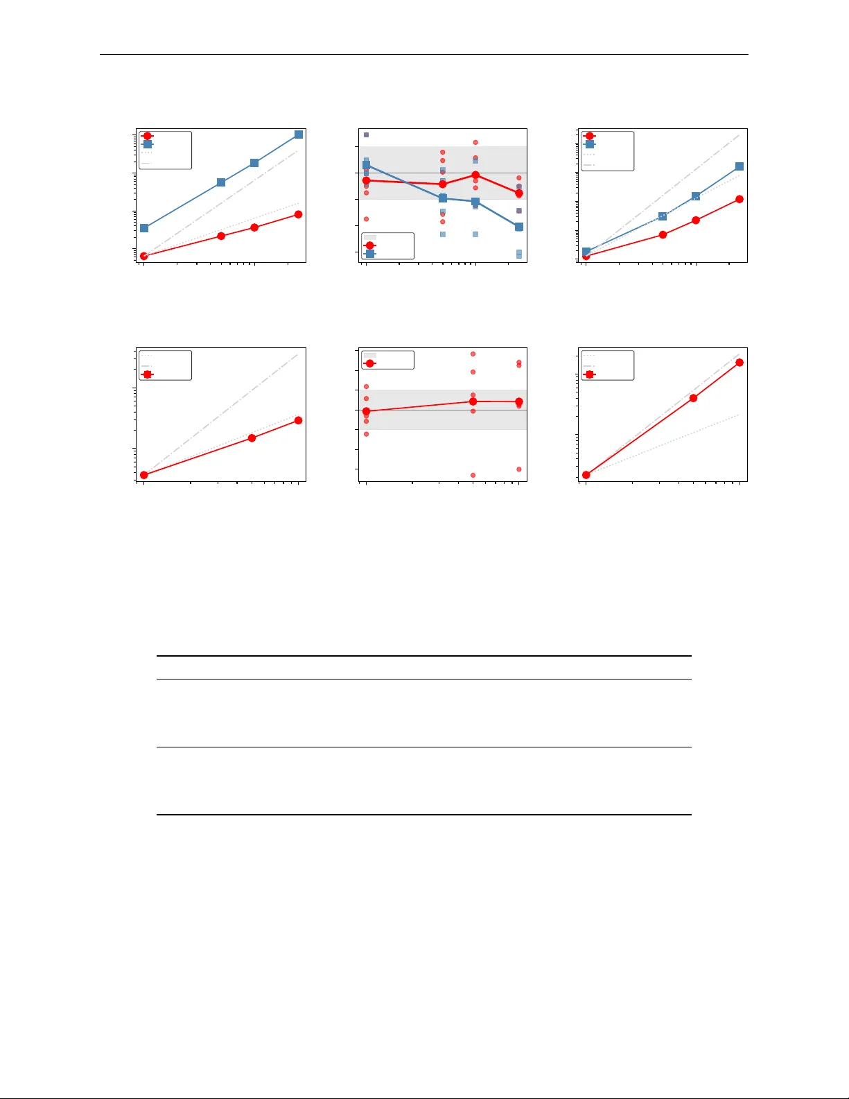
Nested Sampling with Slice-within-Gibbs: Eﬃcient Evidence Calculation fo r Hiera rchical Ba y esian Mo dels Da vid Y allup dy297@c am.ac.uk K avli Institute for Cosmolo gy Cambridge, University of Cambridge Institute of A str onomy, University of Cambridge Abstract W e presen t Nested Sampling with Slice-within-Gibbs (NS-SwiG), an algorithm for Bay esian inference and evidence estimation in high-dimensional mo dels whose likelihoo d admits a factorization, suc h as hierarc hical Bay esian models. W e construct a procedure to sample from the likelihoo d-constrained prior using a Slice-within-Gibbs kernel: an outer up date of h yp erparameters follo w ed b y inner blo ck updates ov er lo cal parameters. A likelihoo d-budget decomp osition cac hes p er-blo ck contributions so that each lo cal up date chec ks feasibility in constan t time rather than recomputing the global constraint at linearly growing cost. This reduces the p er-replacement cost from quadratic to linear in the num b er of groups, and the o v erall algorithmic complexit y from cubic to quadratic under standard assumptions. The decomp osition extends naturally beyond indep endent observ ations, and w e demonstrate this on Marko v-structured latent v ariables. W e ev aluate NS-SwiG on challe nging b enchmarks, demonstrating scalability to thousands of dimensions and accurate evidence estimates even on p osterior geometries where state-of-the-art gradient-based samplers can struggle. 1 Intro duction Nested sampling (Skilling, 2006) has b ecome a cornerstone of Ba yesian inference in the ph ysical sciences (Ash ton et al., 2022; Buchner, 2023). Unlik e Marko v chain Mon te Carlo (MCMC), nested sampling directly estimates the Bay esian evidence Z = R L ( D | θ ) π ( θ ) dθ , enabling rigorous mo del comparison. This is central to hypothesis testing tasks such as comparing physical mo dels, distinguishing signal from noise, or selecting among p opulation mo dels. Practical implementations treat constrained-prior sampling—dra wing from the prior truncated to a lik eliho o d threshold—largely as a blac k-b o x task (F eroz et al., 2009; Handley et al., 2015a; Sp eagle, 2020; Buc hner, 2021), with limited exploitation of mo del-sp eciﬁc factorisation. In high dimensions, the a v ailable constrained MCMC mutation kernels can mix p o orly , often resem bling local random-walk exploration. The dominant paradigm for scaling Bay esian methods to high dimensions is to use the gradient of the tar- get distribution to suppress this random-w alk b eha viour (F earnhead et al., 2024). Gradient-based samplers suc h as Hamiltonian Monte Carlo (HMC) (Neal, 2011) and the No-U-T urn Sampler (NUTS) (Hoﬀman & Gelman, 2014) hav e b ecome ubiquitous general-purp ose inference to ols, and the success of Stan (Carp en- ter et al., 2017) has reinforced a widespread view—particularly among practitioners—that gradien ts are essen tial for scalability . Designing eﬃcient gradient-based samplers for hard lik eliho o d constraints remains c hallenging; existing approac hes for nested sampling (F eroz & Skilling, 2013; Lemos et al., 2023) ha ve not y et demonstrated robust p erformance across generic problem classes (Kroupa et al., 2025), outside settings with additional structure (e.g., log-concav e mo dels amenable to pro ximal metho ds (Cai et al., 2022)). This has left nested sampling view ed as well suited for low-dimensional problems with pathological geometries, but requiring alternatives for high-dimensional inference (Piras et al., 2024). This pap er in tro duces Neste d Sampling with Slic e-within-Gibbs (NS-SwiG), a constrained-sampling inner lo op that exploits the conditional indep endence structure of mo dels with factorised likelihoo ds. Consider a hierarc hical mo del with J groups, lo cal parameters θ j , and shared hyperparameters ψ , where the log- lik eliho o d decomp oses as ℓ ( ψ , { θ j } ) = P J j =1 ℓ j ( θ j , ψ ) . Standard nested sampling chec ks the global constrain t 1 ℓ > ℓ ∗ at every MCMC prop osal, costing O ( J ) p er ev aluation; with O ( J ) parameters requiring up dates, this yields O ( J 2 ) p er replacement. NS-SwiG decomp oses the global constrain t into p er-blo ck budgets chec kable in O (1) , reducing the cost to O ( J ) . This builds on contemporary work reviving interest in co ordinate-wise Metr op olis-within-Gibbs schemes as scalable alternatives to join t-gradient metho ds (Ascolani et al., 2024; Luu et al., 2025). W e em b ed a Slice- within-Gibbs k ernel within a nested sampling outer lo op, targeting the join t constrained prior with blo ck up dates: an outer slice up date of h yp erparameters follow ed b y an inner sweep ov er the J lo cal blo cks. W e demonstrate the scalability this unlo cks on challenging b enchmarks up to d ∼ 2500 dimensions. In summary , w e make the following contributions: (i) Lik eliho o d-budget decomp osition. W e show that the global nested sampling constraint can be decomp osed into p er-blo ck budgets updated in O (1) from a cac hed total, extending naturally to Mark o v-structured latent v ariables where budgets dep end on lo cal neighbourho o ds. (ii) Constrained Slice-within-Gibbs kernel. W e construct an MCMC kernel for the joint constrained prior using blo ck ed slice updates, yielding O ( J ) p er sweep compared to O ( J 2 ) for standard join t-space constrained sampling. (iii) Implemen tation and v alidation. W e provide a fully vectorised JAX implemen tation building on Y allup et al. (2026), v alidate p osterior recov ery against NUTS on four b enchmarks, and demon- strate accurate evidence estimates at scale. W e motiv ate a num b er of immediate applications within astroph ysics, where nested sampling is already widely used for ob ject-level inference problems. The remainder of the pap er is organized as follows. Section 2 reviews nested sampling fundamentals and hierarc hical mo del structure. Section 3 presents NS-SwiG, including the budget decomposition, cac hing strategy , and constrained Slice-within-Gibbs up dates. Section 4 rep orts numerical exp erimen ts v alidating correctness and scaling across four benchmarks. Section 5 discusses limitations, extensions, and practical considerations, and Section 6 concludes. 2 Background Man y high-dimensional Bay esian models are high-dimensional because they comp ose many rep eated lo w- dimensional components. Consider an inference task where J ob jects are observ ed with data D j ; we construct a mo del with lo cal parameters θ j and shared hyperparameters ψ . The likelihoo d factorizes as L ( D | ψ , { θ j } J j =1 ) = J Y j =1 L j ( D j | θ j , ψ ) . (1) Deﬁning ℓ j ( θ j , ψ ) := log p ( D j | θ j , ψ ) , the log-lik eliho o d decomp oses as ℓ ( ψ , { θ j } ) = P J j =1 ℓ j ( θ j , ψ ) . While this is a restricted class of mo dels, it is ubiquitous in mo dern astrophysics and cosmology (Shariﬀ et al., 2016; Leistedt et al., 2016; Mandel et al., 2019). Such mo dels arise naturally when analyzing p opula- tions of ob jects—gravitational-w a v e sources (Thrane & T alb ot, 2019; LIGO Scien tiﬁc Collab oration et al., 2023), sup ernov ae (Gra yling et al., 2024), galaxies (Alsing et al., 2024)—where each observ ation constrains lo cal parameters while shared hyperparameters describ e the p opulation-lev el distribution. In many of these examples, object-level p osteriors can b e multimodal or ha ve inv alid regions of parameter space, making nested sampling a practical solution (Ash ton et al., 2019; Johnson et al., 2021). Ho wev er, this can make p opulation-lev el inference challenging: lifting ob ject-level analyses into a joint gradient-based sampler often compromises the robustness of the ob ject-level inference. This provides domain-speciﬁc motiv ation, but more generally , extracting marginal likelihoo ds for high- dimensional models is broadly relev an t across scientiﬁc domains and remains notoriously challeng- ing (Llorente et al., 2023). In this section we review the necessary background on nested sampling, Metrop olis- within-Gibbs, and hierarchical mo dels. 2 2.1 Nested Sampling Let the full parameter vector b e ϑ ≡ ( ψ , θ 1: J ) ∈ R d with d = d ψ + J d θ , prior densit y π ( ϑ ) , lik eliho o d L ( ϑ ) = p ( D | ϑ ) , log-likelihoo d ℓ ( ϑ ) = log L ( ϑ ) , and evidence Z = Z L ( ϑ ) π ( ϑ ) dϑ. (2) Nested sampling (Skilling, 2006) rewrites this integral using the prior v olume ab ov e a log-likelihoo d threshold, X ( ℓ ) := Z π ( ϑ ) 1 { ℓ ( ϑ ) >ℓ } dϑ ∈ [0 , 1] , (3) and let ℓ ( X ) denote its (generalized) inv erse. Then Z = R 1 0 L ( X ) dX , where L ( X ) = exp( ℓ ( X )) is the lik eliho o d at prior volume X . The algorithm maintains m particles (often called live p oints in the nested sampling literature) approximating dra ws from the c onstr aine d prior at the curren t threshold ℓ ∗ . At eac h iteration it remov es the live point with the smallest log-likelihoo d, accounts for its contribution to Z , and replaces it with a new draw from π ℓ ∗ ( ϑ ) ∝ π ( ϑ ) 1 { ℓ ( ϑ ) >ℓ ∗ } , (4) with X ( ℓ ∗ ) as the normalizing constant. Eﬃciently sampling from (4) is typ ically the dominant cost, ad- dressed by ellipsoidal metho ds (F eroz et al., 2009), slice-based approac hes (Handley et al., 2015a; Neal, 2003). Nested sampling is widely used in the ph ysical sciences for Bay esian model comparison via marginal like- liho o d (evidence) estimation, often in settings with computationally expensive forward models. F rom this p ersp ectiv e it is closely related to Sequen tial Monte Carlo (SMC) samplers for static targets, which estimate normalizing constants using an artiﬁcial sequence of in termediate distributions (Chopin, 2002; Del Moral et al., 2006), often deﬁned b y likelihoo d temp ering/annealing (Neal, 2001). W e do not address p opular scalable approac hes to mo del comparison based on stacking or cross-v alidation (V ehtari et al., 2017; F ong & Holmes, 2019; Y ao et al., 2022). These metho ds primarily address scalability with resp ect to large datasets (e.g., a voiding reﬁts for held-out data) and typically op erate by p ost-pro cessing draws from an existing inference pro cedure; they are therefore not themselv es a sampling technique. 2.2 Metrop olis-within-Gibbs and Hiera rchical Mo dels Gibbs sampling is a classic algorithm for sampling from a join t distribution b y iteratively sampling from the full conditional of each v ariable giv en the others (MacKa y, 2002), often employ ed in situations where the full conditionals are tractable and easy to sample from. Metrop olis-within-Gibbs generalizes the idea of mo ving a subset of parameters whilst ﬁxing others (Chib & Green b erg, 1995). F or challenging conditional distributions, slice sampling (Neal, 2003) within Gibbs-style alternating up dates has b een shown to mix eﬀectiv ely even in high dimension for generalized linear mo dels (Luu et al., 2025). This aligns w ell with tw o asp ects of our setting. First, slice sampling is the dominan t paradigm used for MCMC mutation within nested sampling (Handley et al., 2015a). Second, hierarc hical mo dels are a classic setting for Gibbs sampling (Damien et al., 1999), though practical implementation for general non-conjugate mo dels and large J remains challenging. F or hierarc hical mo dels as in eq. (1), with h yp erparameters ψ ∈ R d ψ and group-sp eciﬁc parameters θ j ∈ R d θ for j = 1 , . . . , J , we assume the prior factorizes as π ( ϑ ) = π ( ψ ) Q j π ( θ j | ψ ) . The joint p osterior is then p ( ψ , θ 1: J | D ) ∝ π ( ψ ) J Y j =1 π ( θ j | ψ ) L j ( D j | θ j , ψ ) . (5) This structure motiv ates sampling (4) using blo ck Gibbs up dates of ψ and each θ j within the constrained sampler. The key scaling issue is the lik eliho o d constrain t chec k ℓ ( ϑ ) > ℓ ∗ : a naive implementation recom- putes (1) from scratch after each blo ck prop osal, costing O ( J ) p er prop osal. Over a swe ep that up dates all 3 J lo cal blo cks, this yields O ( J 2 ) work p er sw eep. By cac hing the current p er-group likelihoo d contributions { ℓ j } J j =1 and their sum, a proposal that c hanges only one blo ck can up date the constrain t in O (1) , reduc- ing the sweep cost to O ( J ) . Additional savings arise when the data lik eliho o d p ( D j | θ j ) do es not dep end on ψ : only the conditional prior π ( θ j | ψ ) needs recomputation during hyperparameter up dates, and this is typically m uc h cheaper than the data lik eliho o d. Kernels of this within-Gibbs type lea ve the full join t target inv ariant (up to MCMC con v ergence), and recent results establish dimension-robust con ve rgence for Metrop olis-within-Gibbs on broad classes of hierarchical mo dels (Ascolani et al., 2024). In standard nested sampling, sampling from the constrained prior t ypically requires MCMC mov es to decor- relate the new sample from its parent. A standard heuristic to take is that adequate decorrelation in practice t ypically requires O ( d ) slice sampling steps, where d is the total parameter dimension (Y allup et al., 2026). F or hierarchical mo dels, d = d ψ + J · d θ , where d ψ and d θ are the h yp erparameter and p er-group lo cal parameter dimensions resp ectiv ely . Each slice step must chec k the likelihoo d constraint, which in the naive implemen tation requires computing the full sum ab ov e at cost O ( J ) . This yields a per-replacement cost of O ( d · J ) = O ( J 2 ) for large J , whic h b ecomes prohibitive for ob ject catalogs with hundreds to thousands of groups. High dimension further exacerbates some issues in constrained slice sampling. Conv ergence b ounds for Hit- and-R un within slice sampling exhibit p olynomial dep endence on dimension, with sp ectral gaps scaling as O ( d − 3 ) for log-concav e targets (Po wer et al., 2024). Moreo ver, a practical strength of nested sampling—its w eak reliance on hand-tuned prop osals—dep ends on representing the geometry of the constrained region us- ing the liv e p oint cloud. As d grows, b oth the MCMC exploration and this geometric adaptation b ecome less eﬀectiv e, comp ounding the computational b ottleneck in hierarc hical settings. Decomp osing high-dimensional constrained sampling into low er-dimensional conditional up dates can substan tially improv e b oth computa- tional cost and mixing. 2.3 Structure-A wa re Inner Kernels in Nested Sampling T wo lines of prior work exploit mo del structure within the nested sampling inner lo op. The ﬁrst is the fast–slow hierarch y of parameters, developed for cosmological likelihoo ds (Lewis, 2013) and implemented in P olyChord (Handley et al., 2015a;b). When the lik eliho o d factors as L ( z , θ ) = L ( f ( ψ ) , θ ) for an exp ensive forw ard mo del z = f ( ψ ) , the inner MCMC can prop ose mov es in the “fast” parameters θ more frequently and cac he the forw ard-mo del ev aluations. This exploits heterogeneous ev aluation costs but do es not decomp ose the lik eliho o d constraint itself. Secondly , Murray et al. (2005) introduced blo ck Gibbs up dates within nested sampling for the Potts mo del, using Swendsen–W ang (Sw endsen & W ang, 1987) cluster mov es as the constrained inner kernel. The random-cluster auxiliary-v ariable augmentation yields tractable conditionals on a lattice, but the construction is speciﬁc to discrete Marko v random ﬁelds and do es not transfer to general con tin uous hierarchical mo dels. Both approaches can b e view ed as sp ecial cases of a common mo del structure-aw are principle: design the nested sampling m utation k ernel comp ositionally , using blo ck ed up dates paired with inner mov es that ex- ploit mo del-sp eciﬁc structure. W e show that this compositional p ersp ective can be made broadly eﬀective at scale b y using a general-purp ose Slice-within-Gibbs constrained sampler as the building block. In the hierarc hical setting w e emphasize, the additive log-likelihoo d further enables a clean transformation of the global lik eliho o d constraint into p er-blo ck budgets that can b e maintained and chec ked in constant time. W e also note that there are man y examples of custom MCMC mo ves in nested sampling targeting sp eciﬁc mo dels, such as the reversible jump (Green, 1995) mo v es of DNest (Brew er & F oreman-Mack ey, 2016). These are mostly p ositioned as improving the mixing of the inner sampler—certainly an intended side eﬀect of the comp ositional p ersp ective we advocate—but do not explicitly target cost and scalability . 3 Metho d and Implementation With the to ols from the previous section established, we presen t the NS-SwiG algorithm, and discuss its implemen tation details. 4 3.1 Nested Sampling Budget Constraint Decomp osition As outlined in eq. (1), we consider a hierarc hical Bay esian mo del with h yp erparameters ψ ∈ R d ψ and J groups, each with local parameters θ j ∈ R d θ . The p er-group log-likelihoo d is ℓ j ( θ j , ψ ) , and the total log- lik eliho o d is the sum ℓ = P J j =1 ℓ j . The central insight of NS-SwiG is that the nested sampling constraint can b e decomp osed p er-group. Fix ψ and { θ j } j  = k , and consider prop osing θ ′ k for group k . The global constraint P J j =1 ℓ j > ℓ ∗ then rearranges to ℓ k ( θ ′ k , ψ ) > B k , B k ≡ ℓ ∗ − S + ℓ k ( θ k , ψ ) , (6) where S = P J j =1 ℓ j ( θ j , ψ ) is the cac hed total log-lik eliho o d at the current state. Equiv alently , B k = ℓ ∗ − P j  = k ℓ j ( θ j , ψ ) . Given S and the current ℓ k , computing the budget requires only O (1) op erations, reducing constrain t-c hec king from O ( J ) to O (1) p er lo cal up date. 1 Similar residual-constraint decomp ositions app ear in co ordinate descent, Gibbs sampling for truncated dis- tributions, and incremental likelihoo d caching (Luu et al., 2025); our con tribution is embedding this idea within nested sampling’s constrained prior, where caching per-group contributions { ℓ j } J j =1 and their sum S enables O (1) incremen tal up dates upon acceptance of an y lo cal proposal. Since B k = ℓ k − ( S − ℓ ∗ ) , the budget equals the current group log-likelihoo d min us the global slack ( S − ℓ ∗ ) . In practice this means w e maintain tw o cac hed quantities: the running total S and a v ector of p er-group log-lik eliho o ds { ℓ j } J j =1 . Upon acceptance of a proposal θ ′ k , the algorithm computes ℓ ′ k = ℓ k ( θ ′ k , ψ ) , up dates S ← S − ℓ k + ℓ ′ k , and stores ℓ ′ k —all in O (1) . A complete sw eep costs O ( J ) , a factor of J improv ement o v er recomputing the full sum at each step. Early in nested sampling, when ℓ ∗ is lo w and slack is large, B k ≪ ℓ k , giving group k freedom to explore. As ℓ ∗ increases and slac k v anishes, B k → ℓ k , forcing each group to concentrate in high-likelihoo d regions, the correct b ehavior for the nested sampling pro cedure. More generally , if the log-lik eliho o d can be written as a sum of lo cal con tributions, then when w e up date a blo c k of v ariables we only need to recompute the terms that actually in volv e that blo c k. The cost of c hecking the nested-sampling likelihoo d constraint for a prop osed blo ck mov e is therefore prop ortional to the num b er of aﬀected terms, rather than to the full data set. This recov ers the iid setting as the b est case (each blo ck touc hes only one term) and the Marko v c hain setting as the next simplest case (each blo ck touc hes only a constant n um b er of neigh b oring terms), whic h we w ork out in section C.6. In the w orst case—when no useful decomp osition is av ailable—ev ery up date requires recomputing the full log-likelihoo d and w e fall back to joint-space nested sampling. 3.2 Constrained Slice-within-Gibbs Kernel With SwiG, we target sampling from the joint constrained prior π ℓ ∗ ( ψ , { θ j } ) ∝ π ( ψ ) J Y j =1 π ( θ j | ψ ) · 1   X j ℓ j > ℓ ∗   (7) via tw o alternating blo ck up dates, eac h implemen ted by slice sampling with stepping-out and shrinkage: Hyp erparameter up date: ψ |{ θ j } . Sample ψ from its full conditional π ℓ ∗ ( ψ |{ θ j } ) ∝ π ( ψ ) J Y j =1 π ( θ j | ψ ) · 1   X j ℓ j ( θ j , ψ ) > ℓ ∗   . (8) The target includes b oth the hyperprior and the conditional priors Q j π ( θ j | ψ ) ; omitting the latter would target the wrong distribution. Eac h slice ev aluation recomputes all J group likelihoo ds, costing O ( J ) . This 1 This decomp osition can b e view ed through the lens of auxiliary budget v ariables { B j } with B j ≤ ℓ j and P j B j ≥ ℓ ∗ , so that the global constraint decomp oses into p er-factor b ounds—analogous to the auxiliary-v ariable constructions of Damien et al. (1999). 5 step can b e rep eated M ψ times p er replacement, with the total cost scaling as O ( M ψ · J ) . F or most reasonable hierarc hical mo dels the hyperparameter space is lo w-dimensional, so we follo w the standard heuristic of ﬁxing this to b e equal to the nu mber of hyperparameters, M ψ = d ψ . Inner sweep: θ j | ψ , θ − j for j = 1 , . . . , J . F or each group j , sample θ j from π ℓ ∗ ( θ j | ψ , θ − j ) ∝ π ( θ j | ψ ) · 1 [ ℓ j ( θ j , ψ ) > B j ] , (9) where the budget B j = ℓ ∗ − S + ℓ j reform ulates the global constraint as a p er-group threshold. Each slice ev aluation requires a single group-lik eliho o d call; since the num b er of slice ev aluations p er up date has low v ariance and is insensitiv e to dimension under standard tuning (Y allup et al., 2026), each lo cal up date costs O (1) in exp ectation. When d θ > 1 , eac h slice step prop oses along a random direction dra wn from the blo c k-diagonal cov ariance estimate (hit-and-run), rather than cycling through co ordinates. Since each lo cal blo c k is typically low-dimensional, w e ﬁx the n um b er of inner slice sampling steps to M θ = d θ . This step comprises a sequential sw eep through all J groups, yielding a total cost of O ( M θ · J ) . The o verall cost of one Gibbs sweep is thus O (( M ψ + M θ ) · J ) , which for ﬁxed M ψ and M θ scales as O ( J ) . The full SwiG replacement step is then giv en in algorithm 2, where w e p erform M total alternating pairs of hyperparameter and lo cal sw eeps. This n umber of repeats is exp osed as a tunable hyperparameter. In theory , M = 1 suﬃces to up date all parameters once; in practice we use M = 5 for more conserv ativ e mixing. Eac h blo ck update is an exact slice-sampling up date targeting the corresp onding full conditional under π ℓ ∗ . Therefore the alternating h yp erparameter update and local sw eep deﬁne a Gibbs k ernel that leav es π ℓ ∗ in v arian t. 3.3 Complete Algo rithm and Implementation With a deﬁned mec hanism to p erform the constrained sampling inner lo op, we further embed this within a v ectorized nested sampling outer lo op. Nested sampling is closely related to SMC (Chopin & Papaspiliopou- los, 2020; Salomone et al., 2024), maintaining m liv e particles appro ximately distributed according to the curren t constrained prior π ℓ ∗ , with ℓ ∗ increasing ov er iterations. These particles can be updated in parallel b y deleting k particles with the lo west lik eliho o ds (thereby raising ℓ ∗ to the new minim um live lik eliho o d) and replacing them with k new samples from the constrained prior, using the pro cedure of section 3.2. The c hoice of k /m is analogous to setting a target Eﬀective Sample Size (ESS) in adaptiv e temp ering SMC metho ds (F earnhead & T aylor, 2010). W e implement NS-SwiG b y extending the Nested Slice Sampling (NSS) framew ork of Y allup et al. (2026), whic h pro vides a v ectorized formulation of nested sampling using Hit-and-Run (Smith, 1984) Slice Sam- pling (Neal, 2003; Rudolf & Ullrich, 2018) for constrained up dates. T uning of the slice sampler is informed b y taking a Mahalanobis-normalized co v ariance estimate of the previous p oint cloud to inform the slice prop osal (Handley et al., 2015a), which we take to b e block-diagonal with one blo ck p er group. The outer lo op is terminated when a suﬃcient level of prior volume compression has o ccurred, such that the ratio of remaining mass in eq. (2) is b elow a ﬁxed threshold. The algorithm is implemented in JAX (Bradbury et al., 2018) within the BlackJAX framework (Cab ezas et al., 2024), and utilizes the comp osable transforms in JAX to parallelize MCMC mov es across particles. 3.4 Complexit y and Scaling The outer lo op of particle metho ds adds to the runtime scaling of the metho ds, but provides many proﬁtable features in return. As these algorithms generically inv olve compression of a prior distribution to a p osterior, there is a cost that scales with the Kullback–Leibler divergence, D KL , b et ween these distributions. F or hier- arc hical mo dels as in eq. (5), the conditional indep endence structure allows decomposition of this divergence in to contributions from the hyperparameters and eac h lo cal blo ck: H = D KL  p ( ψ | D ) ∥ π ( ψ )  + E p ( ψ |D )   J X j =1 D KL  p ( θ j | ψ , D j ) ∥ π ( θ j | ψ )    ≡ H ψ + J X j =1 H j . (10) 6 When eac h group contributes O (1) information, H scales linearly with J , which under standard assumptions implies that the outer iterations scale as O ( J ) (Skilling, 2006). This raises the ov erall complexit y when com bined with the SwiG k ernel of NS-SwiG to O ( J 2 ) , improving ov er the O ( J 3 ) scaling of standard join t- space nested sampling. Under the same standard assumptions the log-evidence error scales as, σ (log ˆ Z ) ≈ p H /m . (11) These rates describ e ideal Mon te Carlo ﬂuctuations; in practice, imp erfect mixing can introduce additional v ariance that dominates the p H /m term. This means that maintaining ﬁxed normalizing constant precision as J grows requires m ∝ J liv e particles. Similar scaling argumen ts apply to SMC metho ds (Beskos et al., 2014), which we describ e in section B. 3.5 Compa rison to MCMC Metho ds The outer-lo op cost detailed in section 3.4 is intrinsic to metho ds that bridge prior to p osterior, and can app ear unfav ourable compared to MCMC metho ds that target the p osterior directly . There are how ever a n um b er of nice features that we gain in return for this cost, namely: • Evidence estimation. Primarily , particle metho ds directly estimate the evidence Z , which is crucial for mo del comparison and h yp othesis testing tasks. MCMC metho ds typically require additional tec hniques such as bridge sampling (Gelman & Meng, 1998) or learned harmonic mean estima- tors (McEw en et al., 2023) to estimate Z , which can b e computationally exp ensiv e and hav e less robust scaling guarantees (Micaletto & V ehtari, 2025). • Conv ergence diagnostics and parallelism. P article metho ds t ypically ha ve a natural parallelism across particles and can lev erage this to assess con vergence (Chopin & Papaspiliopoulos, 2020). Comparable diagnostics for MCMC typically require running m ultiple c hains (V eh tari et al., 2021). Depending on the MCMC scheme, it can b e diﬃcult to fully recoup this cost via parallelization (Hoﬀman et al., 2021; Hoﬀman & Sountso v, 2022; Riou-Durand et al., 2023). • T uning. Particle methods can use the point cloud of particles to implemen t a v ariet y of tuning sc hemes adaptively . A daptive MCMC is notoriously tricky to implement (Andrieu & Thoms, 2008), and in practical settings is instead usually implemen ted as pr etuning with some independent w arm up steps. It is particularly instructiv e to compare SwiG mo ves to Metrop olized HMC steps. Under optimal condi- tions with some assumptions ab out the smo othness of the target, classical optimal-scaling results imply that main taining O (1) acceptance probability requires a leapfrog step size ϵ ∝ d − 1 / 4 (Besk os et al., 2010). In a hi- erarc hical mo del with d ≈ d ψ + J d θ , this suggests a b est-case O (( J d θ ) 1 / 4 ) gradien t ev aluations per eﬀectively indep enden t draw. How ever, each gradient ev aluation of the joint log density aggregates contributions from all J groups, so its cost scales as O ( J ) in the num b er of group log-lik eliho o d ev aluations. Combining these heuristics yields a b est-case computational scaling of O ( J 5 / 4 ) p er eﬀective p osterior draw for global-gradient metho ds. The prior w ork of Luu et al. (2025) established that for generalized linear mo dels, there are cases when Slice-within-Gibbs can outp erform HMC and vice-versa. By lifting this construction into a particle metho d, we target a broader class of inference problems, and explore the p otential for mo del comparison at scale. 4 Numerical Exp eriments W e ev aluate NS-SwiG on four benchmarks, v alidating the metho d’s asymptotic scaling, normalizing constant estimation, and p erformance on challenging Bay esian inference problems. Common settings. Unless otherwise stated, all nested sampling runs use m = 1000 particles, delete k = 50 particles per iteration (batch deletion; see Section C.3 for an ablation), and terminate when log Z live − log Z < − 3 . W e use M = 5 sweeps as a default (see Section C.4 for an ablation), with d ψ h yp erparameter 7 slice steps and d θ lo cal slice steps p er group. W e compare, where appropriate, to some baseline algorithms, with key settings detailed as follows: • NSS: standard nested slice sampling on the join t space, using M × d random-direction slice steps p er replacement, where d is the joint dimension. Otherwise this follows the settings of NS-SwiG for a fair comparison. • SMC-HMC: adaptive-tempered SMC with HMC mutation steps (Buc hholz et al., 2020), using 1000 particles with a target ESS of 0.95 and systematic resampling. Mass matrix and step size are tuned adaptiv ely; full details are given in Section C.1. • NUTS: No-U-T urn Sampler (Hoﬀman & Gelman, 2014) with 4 parallel c hains and window adaptation w arm up (Carp enter et al., 2017). Per-experiment c hain lengths and w armup settings are given in eac h subsection. Ev aluation cost is rep orted in “full-lik eliho o d equiv alents. ” F or NS-SwiG, eac h lo cal update ev aluates a single group log-likelihoo d ℓ j ( θ j , ψ ) ; we count eac h suc h call as 1 /J of a full-likelihoo d ev aluation, so that J single-group calls correspond to one full ev aluation. F or NUTS, each leapfrog step requires one gradient ev aluation and counts as one ev aluation, including warm up. F or SMC-HMC, ev aluations are summed o ver all particles, HMC steps, and temp erature incremen ts. Overheads of gradien t ev aluations are not included as we mostly seek to v alidate general scaling b ehavior (Margossian, 2018). Eﬀectiv e sample size (ESS) is computed as follo ws: for NUTS, we rep ort the minimum bulk ESS across all parameters using the ArviZ library (Kumar et al., 2019); for NS, w e compute ESS from the p osterior imp ortance w eights as describ ed in Y allup et al. (2026); for SMC, w e compute ESS from the recycled particle p o ol across all temp erature steps (Le Thu Nguyen et al., 2014). Ev aluations, runtime, and ESS are av eraged o v er rep eated runs. T ables rep ort log ˆ Z as the mean ov er 5 indep endent seeds ± one standard deviation (seed-to-seed), and ˆ σ is the av erage single-run internal uncertaint y estimator, deriv ed using standard recip es (Skilling, 2006; Chopin & P apaspiliop oulos, 2020). All algorithms are implemen ted using Blac kJAX (Cab ezas et al., 2024), and run on an Apple M1 Studio Max CPU. F urther exp erimental details are provided in Section C. 4.1 Hiera rchical Gaussian Mo del W e ﬁrst ev aluate the p erformance and scaling of NS-SwiG on an idealized target with tractable p osteriors and evidence, primarily to conﬁrm the scaling arguments of b oth the num b er of ev aluations and the normalizing constan t error. W e consider a hierarc hical Gaussian mo del with d ψ = 1 hyperparameter ψ (the population mean) and J groups each with d θ = 1 lo cal parameter θ j , with one observ ation y j p er group: ψ ∼ N ( µ 0 , σ 2 ψ ) , (12) θ j | ψ ∼ N ( ψ , σ 2 θ ) , (13) y j | θ j ∼ N ( θ j , σ 2 obs ) . (14) Marginalizing θ j yields y j | ψ ∼ N ( ψ , τ 2 ) with τ 2 = σ 2 θ + σ 2 obs , and marginalizing ψ then gives the analytic log-evidence. The joint parameter dimension is d = d ψ + J · d θ = 1 + J , and the p osterior information satisﬁes H = O ( J ) . W e use µ 0 = 0 , σ ψ = 10 , σ θ = 2 , and σ obs = 1 , with data generated from ψ = 3 . In this mo del, the observ ation likelihoo d p ( y j | θ j ) is indep endent of ψ , so updating ψ requires recomputing only the conditional priors π ( θ j | ψ ) . Although ψ updates do not require likelihoo d calls, w e force a full recomputation during ψ up dates to em ulate the typical setting where the lik eliho o d depends on hyperparameters. Ev aluation coun ts reﬂect this additional cost. First, we compare NS-SwiG against standard joint sampling in NSS for J ∈ { 10 , 50 , 100 , 250 } and conﬁrm that the prop osed scaling improv ement from O ( J 2 ) to O ( J ) in full-lik eliho o d equiv alents holds (Figure 1a). W e also sho w that the normalizing constant estimate, and internal estimate of the standard error, remain accurate and consistent with the analytic v alue across this range. F or NSS, the estimate of log Z starts 8 T able 1: NS-SwiG vs NSS hierarc hical Gaussian model scaling comparison (results are av eraged ov er 5 rep eated runs with diﬀerent random seeds). Metho d J R untime (s) Ev aluations log Z true log ˆ Z ˆ σ NS-SwiG 10 1 . 3 × 10 0 6 . 3 × 10 5 − 25 . 34 − 25 . 36 ± 0 . 14 0 . 13 NSS 10 1 . 8 × 10 0 3 . 5 × 10 6 − 25 . 30 ± 0 . 09 0 . 13 NS-SwiG 50 7 . 0 × 10 0 2 . 1 × 10 6 − 120 . 64 − 120 . 76 ± 0 . 29 0 . 26 NSS 50 3 . 0 × 10 1 5 . 5 × 10 7 − 120 . 90 ± 0 . 24 0 . 27 NS-SwiG 100 2 . 2 × 10 1 3 . 6 × 10 6 − 228 . 71 − 228 . 74 ± 0 . 30 0 . 34 NSS 100 1 . 5 × 10 2 1 . 8 × 10 8 − 229 . 09 ± 0 . 30 0 . 34 NS-SwiG 250 1 . 2 × 10 2 8 . 0 × 10 6 − 559 . 76 − 560 . 19 ± 0 . 26 0 . 56 NSS 250 1 . 6 × 10 3 1 . 0 × 10 9 − 560 . 82 ± 0 . 48 0 . 52 T able 2: NS-SwiG hierarchical Gaussian mo del extended scaling results (results are av eraged o ver 5 rep eated runs with diﬀerent random seeds). J d R untime (s) Ev aluations log Z true log ˆ Z ˆ σ 100 101 2 . 2 × 10 1 3 . 6 × 10 6 − 228 . 71 − 228 . 74 ± 0 . 30 0 . 34 500 501 4 . 0 × 10 2 1 . 5 × 10 7 − 1097 . 69 − 1097 . 36 ± 1 . 56 0 . 73 1000 1001 1 . 5 × 10 3 2 . 9 × 10 7 − 2204 . 60 − 2204 . 16 ± 1 . 99 1 . 04 to degrade at large J , compatible with the view that the ﬁxed 5 × d rep eats of slice sampling is pro viding insuﬃcien t mixing for multiv ariate slice sampling in h undreds of dimensions. The ev aluation scaling trans- lates into substan tial wall-clock gains at larger J (Figure 1c), though for small J dispatch ov erhead partially masks the asymptotic b ehavior. Numerical results a v eraged ov er 5 rep eated runs are sho wn in T able 1. Second, we scale up to J = 1000 groups ( d = 1001 ), dropping NSS as its runtime b ecomes prohibitiv e. Figures 1d to 1f conﬁrm that O ( J ) scaling in full-lik eliho o d equiv alents holds, and that evidence estimates remain accurate. The observ ed seed-to-seed v ariance of log ˆ Z is sligh tly larger than the av erage in ternal estimator ˆ σ , suggesting a small additional source of mixing error, but the ov erall estimates remain within acceptable precision even at J = 1000 . 4.2 F unnel The funnel distribution introduced by Neal (2003) encapsulates a known pathology that is encountered in man y hierarchical mo dels, namely a strong coupling b et w een hyperparameters and lo cal parameters that creates a funnel-shap ed geometry with v arying lo cal scales. W e use a version with d ψ = 1 , J = 10 , and d θ = 1 (total d = 11 ): ψ ∼ N (0 , σ 2 ψ ) , σ 2 ψ = 9 , (15) θ j | ψ ∼ N (0 , e ψ ) , j = 1 , . . . , J. (16) W e treat the Gaussian conditionals as p er-group likelihoo ds ℓ j = log N ( θ j | 0 , e ψ ) and assign a broad uniform prior θ j ∼ Uniform( − 100 , 100) on each lo cal parameter to ensure supp ort cov ers the funnel’s v arying width. The unnormalized target is therefore π ( ψ ) Q j N ( θ j | 0 , e ψ ) o ver the uniform supp ort, and log Z true = − 52 . 98 is obtained by analytically marginalizing θ j within the uniform b ounds. When ψ is large, the θ j are diﬀuse; when ψ is small (esp ecially negativ e), they concen trate tightly near zero, creating a c hallenging geometry for join t-space samplers. The centered parameterization is a known failure mo de of gradient-based samplers suc h as NUTS, which struggle to explore the funnel without reparameterization (Gorino v a et al., 2019). W e therefore also test a non-centered version: η j ∼ N (0 , 1) with θ j = η j exp( ψ / 2) , which renders the problem w ell-conditioned. 9 10 1 10 2 Number of groups J 10 6 10 7 10 8 10 9 F ull likelihood equiv alents NS-SwiG NSS O ( J ) O ( J 2 ) (a) F ull-lik eliho o d equiv alents: O ( J ) vs. O ( J 2 ) 10 1 10 2 Number of groups J − 3 − 2 − 1 0 1 (log ˆ Z − log Z ) / ˆ σ ± 1 σ NS-SwiG NSS (b) Normalized evidence error 10 1 10 2 Number of groups J 10 0 10 1 10 2 10 3 10 4 Runtime (s) NS-SwiG NSS O ( J 2 ) O ( J 3 ) (c) W all-clock runtime 10 2 10 3 Number of groups J 10 7 10 8 F ull likelihood equiv alents O ( J ) O ( J 2 ) NS-SwiG (d) F ull-lik eliho o d equiv alents ( O ( J ) ) 10 2 10 3 Number of groups J − 3 − 2 − 1 0 1 2 3 (log ˆ Z − log Z ) /σ ± 1 σ NS-SwiG (e) Evidence error vs. J 10 2 10 3 Number of groups J 10 2 10 3 Runtime (s) O ( J ) O ( J 2 ) NS-SwiG (f) W all-clo ck run time vs. J Figure 1: Hierarchical Gaussian model scaling. T op row (a–c): NS-SwiG vs. NSS for J ∈ { 10 , 50 , 100 , 250 } . Bottom row (d–f): NS-SwiG extended scaling to J ∈ { 100 , 500 , 1000 } . T able 3: Neal’s funnel results (results are a veraged ov er 5 repeated runs with diﬀeren t random seeds). log Z true = − 52 . 98 . Metho d R untime (s) Ev aluations ESS ESS/ev al log ˆ Z ˆ σ NS-SwiG (C) 5 . 0 × 10 0 3 . 8 × 10 6 49728 1 . 3 × 10 − 2 − 53 . 03 ± 0 . 10 0 . 18 NSS (C) 1 . 0 × 10 1 2 . 2 × 10 7 49774 2 . 3 × 10 − 3 − 52 . 94 ± 0 . 19 0 . 18 NUTS (C) 3 . 2 × 10 0 2 . 9 × 10 5 40 1 . 4 × 10 − 4 — — SMC-HMC (C) 1 . 0 × 10 0 8 . 0 × 10 5 1560 2 . 0 × 10 − 3 − 56 . 70 ± 0 . 74 0 . 04 NS-SwiG (NC) 3 . 4 × 10 0 2 . 3 × 10 6 7865 3 . 4 × 10 − 3 − 52 . 98 ± 0 . 28 0 . 20 NSS (NC) 6 . 3 × 10 0 1 . 3 × 10 7 7926 6 . 2 × 10 − 4 − 52 . 90 ± 0 . 10 0 . 19 NUTS (NC) 2 . 6 × 10 0 5 . 5 × 10 4 9577 1 . 7 × 10 − 1 — — SMC-HMC (NC) 1 . 0 × 10 0 1 . 0 × 10 6 2602 2 . 6 × 10 − 3 − 53 . 99 ± 1 . 75 0 . 06 W e compare all four algorithms on this b enchmark. NUTS uses 4 c hains of 2000 samples, discarding the ﬁrst 500 as burn-in, with 100 steps of windo w adaptation. Results are shown in T able 3, with the ( ψ , θ 0 ) marginal for the centered parameterization in Figure 2. Only the nested sampling metho ds capture the full funnel geometry in the centered parameterization (Fig- ure 2a). NUTS pro duces numerous div ergen t transitions, conﬁrming the geometry is pathological for HMC. SMC-HMC returns a biased evidence estimate with an in ternal uncertaint y far smaller than the actual error, indicating particle degeneracy during temp ering. Under the non-centered parameterization, all methods p erform well, with NUTS b eing most eﬃcient (Figure 2c). NS-SwiG maintains comparable performance to join t-space NSS while achieving the exp ected scaling improv ement in ev aluations. 10 − 10 . 0 − 7 . 5 − 5 . 0 − 2 . 5 0 . 0 2 . 5 5 . 0 7 . 5 10 . 0 θ − 10 . 0 − 7 . 5 − 5 . 0 − 2 . 5 0 . 0 2 . 5 5 . 0 7 . 5 10 . 0 z 0 NSS NS-SwiG 0 . 00 0 . 05 0 . 10 0 . 15 Density 10 − 2 10 − 1 10 0 Density (a) NS-SwiG and NSS marginals − 10 . 0 − 7 . 5 − 5 . 0 − 2 . 5 0 . 0 2 . 5 5 . 0 7 . 5 10 . 0 θ − 10 . 0 − 7 . 5 − 5 . 0 − 2 . 5 0 . 0 2 . 5 5 . 0 7 . 5 10 . 0 z 0 NUTS SMC-HMC 0 . 0 0 . 2 0 . 4 0 . 6 Density 10 − 2 10 − 1 10 0 Density (b) SMC-HMC and NUTS marginals NS-SwiG NSS NUTS SMC-HMC 10 − 4 10 − 3 10 − 2 10 − 1 ESS / ev al Centered NS-SwiG NSS NUTS SMC-HMC Non-centered (c) ESS p er likelihood ev aluation Figure 2: Neal’s funnel (cen tered parameterization). (a,b) ( ψ , θ 0 ) marginal against analytic contours (grey dashed). (c) ESS p er ev aluation for b oth parameterizations. 4.3 Contextual Eﬀects Mo dels A con textual eﬀects mo del applied to observ ations of radon lev els across Minnesota counties (Gelman & Hill, 2007) is a classic hierarc hical regression example. The dataset comprises 946 observ ations across J = 85 Minnesota counties, obtained from the inference_gym b enchmark suite (Sountso v et al., 2020). This mo del has d ψ = 6 hyperparameters ψ ∈ R 6 (coun t y eﬀect mean and scale, 3 regression weigh ts, observ ation scale) and J = 85 groups each with d θ = 1 lo cal parameter (p er-count y random eﬀects), yielding total dimension d = d ψ + J · d θ = 91 . W e ev aluate b oth centered and non-centered parameterizations, comparing the performance of all algorithms. NUTS uses 4 chains of 5000 samples with 1000 warm up steps, discarding the ﬁrst 1000 as burn-in. T o assess p osterior sample qualit y , w e compute the maximum mean discrepancy (MMD) (Gretton et al., 2012) on the join t hyperparameter distribution using a Gaussian k ernel with data-dep endent bandwidth (see Section C.2), against an indep enden t long-run non-cen tered NUTS reference (4 chains, 50 000 p ost-warm up samples). The results are shown in T able 4, with the ESS p er ev aluation shown in Figure 3a. NS-SwiG yields accurate p osterior marginals and evidence estimates in b oth parameterizations. The centered parameterization is more challenging: NS-SwiG shows higher seed-to-seed v ariance, but the centered estimate ( − 1132 . 7 ± 2 . 1 ) is consisten t with the non-cen tered estimates from b oth NS-SwiG ( − 1130 . 0 ± 0 . 1 ) and SMC- HMC ( − 1130 . 5 ± 0 . 3 ), suggesting the NS-SwiG centered estimate is unbiased; note that ˆ σ underestimates the true v ariance here. In con trast, SMC-HMC exhibits a ∼ 5 nat discrepancy in the cen tered case ( − 1127 . 6 ± 0 . 4 ), with an internal uncertaint y far smaller than the actual error, indicating particle degeneracy during temp ering. SMC-HMC also sho ws signs of particle div ersity collapse in the non-cen tered case: the recycled ESS ( ∼ 1000 , comparable to m ) and elev ated MMD relative to the NUTS reference suggest insuﬃcien t mixing ev en in this b etter-conditioned geometry . While NUTS is more eﬃcient for p osterior sampling in the non- 11 T able 4: Radon con textual eﬀects results (results are a veraged ov er 5 rep eated runs with diﬀerent random seeds). P arenthesized MMD v alues indicate self-comparison of the NUTS NC reference. Metho d R untime (s) Ev aluations ESS ESS/ev al log ˆ Z ˆ σ MMD NS-SwiG (C) 1 . 6 × 10 2 1 . 0 × 10 7 17686 1 . 7 × 10 − 3 − 1132 . 71 ± 2 . 12 0 . 21 2 . 1 × 10 − 3 NUTS (C) 7 . 2 × 10 0 4 . 1 × 10 5 1027 2 . 5 × 10 − 3 — — 1 . 4 × 10 − 3 SMC-HMC (C) 3 . 2 × 10 1 1 . 6 × 10 7 1056 6 . 5 × 10 − 5 − 1127 . 63 ± 0 . 44 0 . 06 1 . 5 × 10 − 3 NS-SwiG (NC) 1 . 5 × 10 2 9 . 4 × 10 6 17012 1 . 8 × 10 − 3 − 1129 . 99 ± 0 . 06 0 . 20 1 . 4 × 10 − 3 NUTS (NC) 7 . 3 × 10 0 4 . 4 × 10 5 4112 9 . 4 × 10 − 3 — — ( 1 . 2 × 10 − 3 ) SMC-HMC (NC) 3 . 4 × 10 1 1 . 7 × 10 7 980 5 . 8 × 10 − 5 − 1130 . 46 ± 0 . 34 0 . 06 3 . 3 × 10 − 3 cen tered parameterization (higher ESS/ev al and faster run time), NS-SwiG remains practical and additionally pro vides evidence estimates. 4.4 Sto chastic V olatility As a ﬁnal test w e consider a sto chastic volatilit y (SV) mo del (Kim et al., 1998) on S&P 500, another standard b enc hmark from Sountso v et al. (2020) used for testing samplers at scale. SV models are often treated as a state-space model and tackled with particle ﬁltering/SMC methods that exploit the model’s sequen tial structure (Andrieu et al., 2010; Chopin et al., 2013). W e employ this mo del as a stress-test for scaling to high-dimensional joint inference, noting that sp ecialized particle metho ds for mo dels with this structure are a v ailable. Applying the SwiG kernel requires accounting for the Mark o v structure of the latent v ariables, whic h breaks the conditional indep endence underlying the budget decomposition. W e extend the implementation to main tain local budgets for each block and its neigh b ours, so that feasibilit y chec ks remain O (1) (details in Section C.6). This necessitates the centered parameterization, as the non-centered version renders the lik eliho o d non-local, breaking the budget decomposition. Here J denotes the n umber of time steps (returns), pla ying the same role as the num b er of groups in previous exp eriments. W e consider J = 100 (small) and J = 2516 (full series). The mo del has d ψ = 3 h yp erparameters ψ ∈ R 3 (p ersistence β , level µ , volatilit y-of- v olatilit y σ ) and J latent log-v olatilities ( d θ = 1 ), giving total dimension d = d ψ + J = { 103 , 2519 } . W e compare NS-SwiG (cen tered) against NUTS in b oth parameterizations (4 chains, 100 000 p ost-w armup samples, 10 000 w arm up steps discarded). SMC-HMC is omitted: the extreme v ariance in log-lik eliho o d under the prior prev en ted reliable initialization of the temp ering sc hedule, and mo difying the prior to address this would compromise the p oin t of computing evidences. MMD is computed on the joint hyperparameter distribution using the same Gaussian kernel as in Section 4.3. Results are shown in T able 5 and Figures 3b and 3c. F or J = 100 , NUTS in the non-cen tered parameterization pro duces frequen t divergen t transitions, indicating that the non-cen tered transformation introduces problematic geometry for the AR(1) structure. The cen- tered parameterization is b etter b ehav ed, with higher ESS and no divergences. NS-SwiG pro duces accurate p osterior marginals (Figure 6) and provides evidence estimates, while requiring few er ev aluations and less w all-clo c k time than either NUTS v arian t. F or the full series ( J = 2516 , d = 2519 ), b oth NUTS parame- terizations pro duce zero divergences and perform well, suggesting the additional dimensionalit y regularizes the geometry . All metho ds pro duce consistent MMD v alues ( ∼ 10 − 3 ), indicating NS-SwiG reco v ers accurate p osteriors even at this scale. This motiv ates further extensions to exploit Mark ov structure more explicitly within the NS-SwiG framework. 5 Discussion The line of inquiry presen ted in this pap er w as motiv ated b y t w o main prior threads of work: ﬁrstly the dif- ﬁcult y noted in constructing a robust, general-purpose gradien t-based c onstr aine d sampler, w ell summarized b y Kroupa et al. (2025), and secondly the retrosp ective observ ation that for mo dels with factorizable graph 12 T able 5: Stochastic volatilit y (S&P 500) results (results are av eraged ov er 5 repeated runs with diﬀerent random seeds). Paren thesized MMD v alues indicate self-comparison of the NUTS NC reference. Metho d R untime (s) Ev aluations ESS MMD log ˆ Z d = 103 NUTS (NC) 1 . 0 × 10 2 13 . 8 × 10 6 6 . 4 × 10 3 (1 . 0 × 10 − 3 ) – NUTS (C) 78 14 . 2 × 10 6 14 . 7 × 10 3 1 . 0 × 10 − 3 – NS-SwiG (C) 20 2 . 9 × 10 6 11 . 9 × 10 3 1 . 1 × 10 − 3 − 573 . 4 ± 0 . 1 d = 2519 NUTS (NC) 1 . 0 × 10 3 14 . 6 × 10 6 51 . 3 × 10 3 (1 . 1 × 10 − 3 ) – NUTS (C) 1 . 2 × 10 3 35 . 0 × 10 6 2 . 0 × 10 3 8 . 9 × 10 − 4 – NS-SwiG (C) 4 . 4 × 10 3 30 . 5 × 10 6 11 . 1 × 10 3 1 . 5 × 10 − 3 − 10535 . 5 ± 0 . 5 NS-SwiG NUTS SMC-HMC 10 − 4 10 − 3 10 − 2 ESS / eval Centered NS-SwiG NUTS SMC-HMC Non-centered (a) Radon mo del NS-SwiG (C) NUTS (C) NUTS (NC) 10 − 3 ESS / eval (b) SV small ( d = 103 ) NS-SwiG (C) NUTS (C) NUTS (NC) 10 − 4 10 − 3 ESS / eval (c) SV full ( d = 2519 ) Figure 3: ESS p er likelihoo d ev aluation across b enchmarks. structure, sampling can b e made highly scalable just b y exploiting this mo del structure (Luu et al., 2025). W e demonstrated that combining these insights, b y constructing a Slice-within-Gibbs kernel that exploits factorised likelihoo d structure, enables nested sampling to scale to high-dimensional problems while retaining the core adv an tages of direct evidence estimation and robustness to c hallenging p osterior geometries. By cac hing p er-group likelihoo d contributions, the algorithm reduces the likelihoo d-ev aluation cost p er Gibbs sw eep from O ( J 2 ) to O ( J ) for J groups, and is a step tow ards impro ving nested sampling analyses currently hitting this quadratic cost (Johnson et al., 20 24; Lovic k et al., 2025). Empirically , we pro vided a comparison to multiple state-of-the-art baselines using common (and mostly conserv ativ e) settings. The exp eriments demonstrate that a SwiG up date can yield a comp etitive inference k ernel even at scale, with particularly strong p erformance in estimating normalizing constants, a notoriously diﬃcult task at high dimension, and on c hallenging geometries without reparameterisation. Limitations The main limitation of this w ork is the need for some kind of factorised structure in the lik eliho o d, which is a common but not universal feature of high dimensional problems. The approach is most comp elling when lo cal blo cks are low-dimensional (so that slice-based lo cal mov es mix well) and when global structure can b e cached cheaply . If b oth the hyperparameters and each lo cal blo ck are high-dimensional, then the basic Slice-within-Gibbs strategy ma y not b e the right inner kernel, and collapsing or alternativ e constrained prop osals may b e preferable. Another practical limitation for nested sampling at high dimension is not only the cost p er constrained step, but also the num b er of particles m required to maintain accurate evidence estimates as dimensionality grows. While NS-SwiG reduces the cost of generating constrained prior samples, and our v ectorised implemen tation can amortise likelihoo d computation across groups and particles, the particle requirement can still b ecome the dominant cost beyond d ≳ 10 3 . This motiv ates exploring strategies that reduce the eﬀectiv e dimension seen by the sampler. More broadly , nested sampling accuracy dep ends on the quality of constrained samples: when the inner MCMC do es not mix adequately within the likelihoo d con tour, evidence estimates can be biased. This is a general concern for any nested sampling implementation, and motiv ates monitoring diagnostics such as the stabilit y of log Z estimates with resp ect to the n um b er of inner MCMC steps. Additionally , caching per- 13 group likelihoo d con tributions incurs O ( mJ ) memory ov erhead, which can b ecome limiting on accelerators at the scales we target. Extensions A w ell motiv ated extension that addresses the t w o limitations ab ov e is to adopt pseudo- marginal or more generally c ol lapse d approaches for subsets of parameters so that the constrained inner loop op erates on a lo wer-dimensional representation. This is particularly natural in ligh t of observ ations suc h as the full SV mo del, where increasing the latent dimension actually regularizes the problem, rendering it b etter approximated by conditional Gaussian assumptions that would b e natural in a collapsed sampler. Another natural case we do not explore is strongly heterogeneous compute costs across blo cks, as was noted for the classic implemen tation of fast-slow . It is natural to consider the blo ck ed Gibbs approach as applicable to suc h problems, how ever, without explicit factorization of the lik eliho o d, correlations b etw een nominally “fast” and “slow” comp onents could lead to more challenging dynamics to explore. Finally , we emphasise that the strong p erformance of NS-SwiG on non-linear, non-Gaussian examples (in- cluding centered parameterisations) is suggestive of more than just an alternative to reparameterisation. In man y p otential application domains—especially those inv olving physical forward mo dels—there may b e no clear a priori transformation that reliably impro ves conditioning. F urther v alidating the p erformance of nested sampling at scale on such problems is an interesting direction for future work, and may b e a domain where NS-SwiG is particularly comp elling. 6 Conclusion W e presented NS-SwiG, a nested sampling algorithm for hierarchical Ba yesian inference that reduces the cost of eac h live-point replacement from O ( J 2 ) to O ( J ) (in full-lik eliho o d-ev aluation equiv alen ts), where J is the num b er of groups. The k ey idea is a decomp osition of the likelihoo d-threshold constraint that allo ws eac h lo cal blo ck up date to che ck feasibility in O (1) rather than O ( J ) time. A cross b enc hmarks, we v alidate the resulting scaling and sho w that NS-SwiG enables robust, gradient-free p osterior sampling and evidence estimation in regimes where gradient-based samplers can b e unreliable. The strength of this approach comes primarily from exploiting known factorization structure in the likeli- ho o d, which is not guaranteed in all inference problems. Notable coun terexamples that require a fully joint treatmen t of the parameters include sampling molecular conﬁgurations (Párta y et al., 2014), an area that has seen activ e work on neural-netw ork-based learning of full joint conﬁgurations (e.g., Akhound-Sadegh et al. (2024)). Ev en in such settings, there is often low er-dimensional structure that can b e factorized out, such as collectiv e v ariables in molecular systems (F röhlking et al., 2025). F raming the problem as discov ering suc h lo w-dimensional structure when it is not known a priori, rather than inheriting the unfav orable scaling of fully joint sampling, is an interesting direction for future work. P articularly within astrophysics, where nested sampling is already extremely p opular, scaling challenges of existing inference pip elines ab ound. As astronomical catalogs contin ue to grow—with curren t and future gra vitational-w a v e detectors, large-scale surv eys of galaxies and galaxy clusters—metho ds that scale eﬃ- cien tly with catalog size while preserving access to the evidence b ecome increasingly imp ortant. NS-SwiG pro vides b oth p osterior samples and Bay esian evidence in a single run, making nested sampling practical for large-scale hierarc hical problems where scalable inference and rigorous mo del comparison are b oth required. A cknowledgments The author thanks Will Handley for useful discussions. The author was supp orted by the research environ- men t and infrastructure of the Handley Lab at the Universit y of Cambridge. The author used Op enAI GPT 5.2 to reﬁne p ortions of the draft, and Claude Opus 4.5 was used in reﬁning the co de. The author takes full resp onsibilit y for the ﬁnal conten t. 14 Co de and Data Availabilit y The algorithm co de and example scripts to repro duce the exp eriments in this pap er are av ailable at https: //github.com/yallup/swig References T ara Akhound-Sadegh, Jarrid Rector-Bro oks, A vishek Jo ey Bose, Sarthak Mittal, P ablo Lemos, Cheng- Hao Liu, Marcin Sendera, Siamak Rav anbakhsh, Gauthier Gidel, Y osh ua Bengio, Nik olay Malkin, and Alexander T ong. Iterated denoising energy matc hing for sampling from b oltzmann densities, 2024. Justin Alsing, Stephen Thorp, Sinan Deger, Hirany a V. P eiris, Boris Leistedt, Daniel Mortlock, and Jo el Leja. pop-cosmos: A Comprehensive Picture of the Galaxy Population from COSMOS Data. A str ophys. J. Suppl. Ser. , 274(1):12, Septem b er 2024. doi: 10.3847/1538- 4365/ad5c69. Christophe Andrieu and Johannes Thoms. A tutorial on adaptive MCMC. Statistics and Computing , 18(4): 343–373, December 2008. ISSN 1573-1375. doi: 10.1007/s11222- 008- 9110- y. URL https://doi.org/10. 1007/s11222- 008- 9110- y . Christophe Andrieu, Arnaud Doucet, and Roman Holenstein. P article Marko v c hain Monte Carlo metho ds. J. R. Stat. So c. Ser. B , 72(3):269–342, 2010. doi: 10.1111/j.1467- 9868.2009.00736.x. Filipp o Ascolani, Gareth O. Rob erts, and Giacomo Zanella. Scalability of Metrop olis-within-Gibbs schemes for high-dimensional Bay esian mo dels, 2024. Gregory Ashton et al. BILBY: A user-friendly Bay esian inference library for gravitational-w av e astronom y. A str ophys. J. Suppl. , 241(2):27, 2019. doi: 10.3847/1538- 4365/ab06fc. Gregory Ash ton et al. Nested sampling for physical scientists. Nat. R ev. Metho ds Primers , 2:39, 2022. doi: 10.1038/s43586- 022- 00121- x . Alexandros Beskos, Natesh S. Pillai, Gareth O. Rob erts, Jesus M. Sanz-Serna, and Andrew M. Stuart. Optimal tuning of the hybrid monte-carlo algorithm, 2010. URL . Alexandros Beskos, Dan Crisan, and Ajay Jasra. On the stabilit y of sequen tial Monte Carlo metho ds in high dimensions. The A nnals of A pplie d Pr ob ability , 24(4):1396–1445, 2014. doi: 10.1214/13- AAP951. James Bradbury , Ro y F rostig, Peter Ha wkins, Matthew James Johnson, Chris Leary , Dougal Maclaurin, George Necula, Adam P aszke, Jake V anderPlas, Skye W anderman-Milne, and Qiao Zhang. JAX: comp os- able transformations of Python+NumPy programs. http://github.com/jax- ml/jax , 2018. Brendon J. Brewer and Daniel F oreman-Mac key . DNest4: Diﬀusive Nested Sampling in C++ and Python. 6 2016. Alexander Buc hholz, Nicolas Chopin, and Pierre E. Jacob. A daptive tuning of hamiltonian mon te carlo within sequential monte carlo, 2020. URL . Johannes Buchner. Ultranest – a robust, general purp ose ba y esian inference engine, 2021. URL https: //arxiv.org/abs/2101.09604 . Johannes Buchner. Nested sampling metho ds. Stat. Surv. , 17:169–215, 2023. doi: 10.1214/23- SS144. Alb erto Cabezas, Adrien Corenﬂos, Junp eng Lao, and Rémi Louf. BlackJAX: Comp osable Bay esian inference in JAX, 2024. Xiaohao Cai, Jason D. McEw en, and Marcelo P ereyra. Pro ximal nested sampling for high-dimensional ba y esian mo del selection. Statistics and Computing , 32(5), Octob er 2022. ISSN 1573-1375. doi: 10.1007/ s11222- 022- 10152- 9. URL http://dx.doi.org/10.1007/s11222- 022- 10152- 9 . 15 Bob Carpenter, Andrew Gelman, Matthew D. Hoﬀman, Daniel Lee, Ben Goo drich, Mic hael Betancourt, Marcus Brubaker, Jiqiang Guo, Peter Li, and Allen Riddell. Stan: A probabilistic programming language. J. Stat. Softw. , 76(1), 2017. doi: 10.18637/jss.v076.i01. Siddhartha Chib and Edward Greenberg. Understanding the Metrop olis-Hastings Algorithm. The A meric an Statistician , 49(4):327–335, 1995. ISSN 0003-1305. doi: 10.2307/2684568. URL https://www.jstor. org/stable/2684568 . N. Chopin and O. Papaspiliopoulos. A n Intr o duction to Se quential Monte Carlo . Springer Series in Statistics. Springer International Publishing, 2020. ISBN 9783030478452. URL https://books.google.co.uk/ books?id=ZZEAEAAAQBAJ . Nicolas Chopin. A Sequen tial P article Filter Metho d for Static Mo dels. Biometrika , 89(3):539–551, 2002. ISSN 0006-3444. URL https://www.jstor.org/stable/4140600 . Nicolas Chopin. Central limit theorem for sequential Monte Carlo metho ds and its application to Bay esian inference. The A nnals of Statistics , 32(6):2385–2411, 2004. Nicolas Chopin, Pierre E. Jacob, and Omiros Papaspiliopoulos. SMC 2 : an eﬃcient algorithm for sequen tial analysis of state space mo dels. J. R. Stat. So c. Ser. B , 75(3):397–426, 2013. doi: 10.1111/j.1467- 9868. 2012.01046.x. P aul Damien, Jon W akeﬁeld, and Stephen W alker. Gibbs Sampling for Bay esian Non-Conjugate and Hierar- c hical Mo dels by Using Auxiliary V ariables. Journal of the R oyal Statistic al So ciety. Series B (Statistic al Metho dolo gy) , 61(2):331–344, 1999. ISSN 1369-7412. URL https://www.jstor.org/stable/2680644 . Pierre Del Moral. F eynman–K ac F ormulae: Gene alo gic al and Inter acting Particle Systems with A pplic ations . Probabilit y and Its Applications. Springer, 2004. Pierre Del Moral, Arnaud Doucet, and Ajay Jasra. Sequen tial Mon te Carlo samplers. J. R. Stat. So c. Ser. B , 68(3):411–436, 2006. doi: 10.1111/j.1467- 9868.2006.00553.x. P aul F earnhead and Benjamin M. T aylor. An adaptive sequen tial Monte Carlo sampler, 2010. P aul F earnhead, Christopher Nemeth, Chris J. Oates, and Chris Sherlo ck. Scalable monte carlo for bay esian learning, 2024. URL . F. F eroz, M. P . Hobson, and M. Bridges. MultiNest: an eﬃcien t and robust Ba yesian inference tool for cosmology and particle ph ysics. Mon. Not. R. A str on. So c. , 398(4):1601–1614, 2009. doi: 10.1111/j. 1365- 2966.2009.14548.x . F arhan F eroz and John Skilling. Exploring multi-modal distributions with nested sampling. In AIP Confer- enc e Pr o c e e dings . AIP , 2013. doi: 10.1063/1.4819989. URL http://dx.doi.org/10.1063/1.4819989 . Edwin F ong and Chris Holmes. On the marginal likelihoo d and cross-v alidation. arXiv pr eprint arXiv:1905.08737 , 2019. Thorb en F röhlking, Simone Aureli, and F rancesco Luigi Gerv asio. Learning committor-consistent collective v ariables. 5(7):520–521, 2025. ISSN 2662-8457. doi: 10.1038/s43588- 025- 00834- 5. URL https://doi. org/10.1038/s43588- 025- 00834- 5 . Andrew. Gelman and Jennifer Hill. Data analysis using r e gr ession and multilevel/hier ar chic al mo dels / A ndr ew Gelman, Jennifer Hil l. Analytical metho ds for so cial research. Cam bridge Univ ersity Press, Cam- bridge ;, 2007. ISBN 978-0-511-76508-7. Publication Title: Data analysis using regression and multi- lev el/hierarc hical mo dels. Andrew Gelman and Xiao-Li Meng. Sim ulating normalizing constan ts: from imp or- tance sampling to bridge sampling to path sampling. Statistic al Scienc e , 13(2): 163–185, May 1998. ISSN 0883-4237, 2168-8745. doi: 10.1214/ss/1028905934. URL https://projecteuclid.org/journals/statistical- science/volume- 13/issue- 2/ 16 Simulating- normalizing- constants- - from- importance- sampling- to- bridge- sampling/10.1214/ ss/1028905934.full . W alter R. Gilks and Carlo Berzuini. F ollowing a mo ving target—Monte Carlo inference for dynamic Bay esian mo dels. Journal of the R oyal Statistic al So ciety: Series B (Statistic al Metho dolo gy) , 63(1):127–146, 2001. ISSN 1467-9868. doi: 10.1111/1467- 9868.00280. URL https://onlinelibrary.wiley.com/doi/abs/10. 1111/1467- 9868.00280 . _eprint: h ttps://rss.onlinelibrary .wiley .com/doi/pdf/10.1111/1467-9868.00280. Maria I. Gorinov a, Da v e Mo ore, and Matthew D. Hoﬀman. A utomatic reparameterisation of probabilistic programs, 2019. URL . Matthew Grayling, Stephen Thorp, Kaisey S. Mandel, Suhail Dhaw an, Ana Soﬁa M. Uzso y , Benjamin M. Bo yd, Erin E. Hay es, and Sam M. W ard. Scalable hierarchical ba yesn inference: In vestigating dep endence of sn ia host galaxy dust prop erties on stellar mass and redshift, 2024. URL 2401.08755 . P eter J. Green. Rev ersible Jump Marko v Chain Monte Carlo Computation and Bay esian Mo del Deter- mination. Biometrika , 82(4):711–732, 1995. ISSN 0006-3444. doi: 10.2307/2337340. URL https: //www.jstor.org/stable/2337340 . Arth ur Gretton, Karsten M. Borgwardt, Malte J. Rasc h, Bernhard Sc hölkopf, and Alexander Smola. A k ernel t w o-sample test. Journal of Machine L e arning R ese ar ch , 13(25):723–773, 2012. URL http://jmlr.org/ papers/v13/gretton12a.html . W. J. Handley , M. P . Hobson, and A. N. Lasenb y . polychord: next-generation nested sampling. Mon. Not. R. A str on. So c. , 453(4):4384–4398, 2015a. doi: 10.1093/mnras/stv1911. W. J. Handley , M. P . Hobson, and A. N. Lasenb y . polychord: nested sampling for cosmology . Mon. Not. R. A str on. So c. L ett. , 450(1):L61–L65, 2015b. doi: 10.1093/mnrasl/slv047. Matthew Hoﬀman, Alexey Radul, and Pa vel Sountso v. An adaptiv e-mcmc sc heme for setting tra jectory lengths in hamiltonian monte carlo. In Arindam Banerjee and Kenji F ukumizu (eds.), Pr o c e e dings of The 24th International Confer enc e on A rtiﬁcial Intel ligenc e and Statistics , volume 130 of Pr o c e e dings of Machine L e arning R ese ar ch , pp. 3907–3915. PMLR, 13–15 Apr 2021. URL https://proceedings.mlr. press/v130/hoffman21a.html . Matthew D. Hoﬀman and Andrew Gelman. The No-U-T urn sampler: Adaptiv ely setting path lengths in Hamiltonian Monte Carlo. J. Mach. L e arn. R es. , 15(47):1593–1623, 2014. URL http://jmlr.org/ papers/v15/hoffman14a.html . Matthew D. Hoﬀman and P a v el Soun tsov. T uning-free generalized hamiltonian mon te carlo. In Gustau Camps-V alls, F rancisco J. R. R uiz, and Isab el V alera (eds.), Pr o c e e dings of The 25th International Confer- enc e on A rtiﬁcial Intel ligenc e and Statistics , volume 151 of Pr o c e e dings of Machine L e arning R ese ar ch , pp. 7799–7813. PMLR, 28–30 Mar 2022. URL https://proceedings.mlr.press/v151/hoffman22a.html . Aaron D. Johnson et al. NANOGrav 15-y ear gravitational-w av e bac kground metho ds. Phys. R ev. D , 109 (10):103012, 2024. doi: 10.1103/PhysRevD.109.103012. Benjamin D. Johnson, Jo el Leja, Charlie Conroy, and Joshua S. Sp eagle. Stellar Population Inference with Prosp ector. A str ophys. J. Suppl. Ser. , 254(2):22, June 2021. doi: 10.3847/1538- 4365/ab ef67. Sang jo on Kim, Neil Shephard, and Siddhartha Chib. Sto chastic v olatility: Likelihoo d inference and com- parison with ARCH mo dels. R ev. Ec on. Stud. , 65(3):361–393, 1998. doi: 10.1111/1467- 937X.00050. Nam u Kroupa, Gáb or Csányi, and Will Handley . Resonances in reﬂective hamiltonian monte carlo. Physic al R eview E , 111(4):045308, 2025. Ra vin Kumar, Colin Carroll, Ari Hartikainen, and Osv aldo Martin. Arviz a uniﬁed library for exploratory analysis of bay esian mo dels in python. Journal of Op en Sour c e Softwar e , 4(33):1143, 2019. doi: 10.21105/ joss.01143. URL https://doi.org/10.21105/joss.01143 . 17 Thi Le Thu Nguy en, F rancois Septier, Gareth W. Peters, and Y v es Delignon. Improving SMC sampler estimate b y recycling all past simulated particles. In 2014 IEEE W orkshop on Statistic al Signal Pr o c essing (SSP) , pp. 117–120, June 2014. doi: 10.1109/SSP .2014.6884589. URL https://ieeexplore.ieee.org/ document/6884589 . ISSN: 2373-0803. Boris Leistedt, Daniel J. Mortlo ck, and Hirany a V. Peiris. Hierarchical Bay esian inference of galaxy redshift distributions from photometric surveys. MNRAS , 460(4):4258–4267, A ugust 2016. doi: 10.1093/mnras/ st w1304. P ablo Lemos, Nik olay Malkin, Will Handley , Y osh ua Bengio, Y ashar Heza veh, and Laurence P erreault- Lev asseur. Improving gradient-guided nested sampling for posterior inference, 2023. URL https:// arxiv.org/abs/2312.03911 . An ton y Lewis. Eﬃcien t sampling of fast and slow cosmological parameters. Phys. R ev. D , 87(10):103529, 2013. doi: 10.1103/Ph ysRevD.87.103529. LIGO Scien tiﬁc Collab oration, Virgo Collab oration, and KAGRA Collaboration. P opulation of merging compact binaries inferred using gravitational w av es through GWTC-3. Phys. R ev. X , 13:011048, 2023. doi: 10.1103/Ph ysRevX.13.011048. F redrik Lindsten, Michael I. Jordan, and Thomas B. Schön. Particle gibbs with ancestor sampling, 2014. URL . F. Llorente, L. Martino, D. Delgado, and J. Lóp ez-San tiago. Marginal lik eliho o d computation for mo del selection and hypothesis testing: An extensive review. SIAM R eview , 65(1):3–58, 2023. T oby Lovic k, David Y allup, Davide Piras, Alessio Spurio Mancini, and Will Handley . High-Dimensional Ba y esian Mo del Comparison in Cosmology with GPU-accelerated Nested Sampling and Neural Emulators. 9 2025. Son Luu, Zuheng Xu, Nikola Surjanovic, Miguel Biron-Lattes, T revor Campb ell, and Alexandre Bouchard- Côté. Is Gibbs sampling faster than Hamiltonian Mon te Carlo on GLMs? In Pr o c e e dings of the 28th International Confer enc e on A rtiﬁcial Intel ligenc e and Statistics (AIST A TS) , 2025. Da vid J. C. MacKay . Information The ory, Infer enc e & L e arning A lgorithms . Cambridge Univ ersit y Press, USA, 2002. ISBN 0521642981. Ily a Mandel, Will M. F arr, and Jonathan R. Gair. Extracting distribution parameters from m ultiple uncertain observ ations with selection biases. Mon. Not. R. A str on. So c. , 486(1):1086–1093, 2019. doi: 10.1093/ mnras/stz896. Charles C. Margossian. A review of automatic diﬀerentiation and its eﬃcien t implemen tation. CoRR , abs/1811.05031, 2018. URL . Jason D. McEwen, Christopher G. R. W allis, Matthew A. Price, and Alessio Spurio Mancini. Machine learning assisted bay esian mo del comparison: learn t harmonic mean estimator, 2023. URL https:// arxiv.org/abs/2111.12720 . Giorgio Micaletto and Aki V ehtari. Bridge sampling diagnostics, 2025. URL 2508.14487 . Iain Murray and Matthew Graham. Pseudo-marginal slice sampling. In Arth ur Gretton and Christian C. Rob ert (eds.), Pr o c e e dings of the 19th International Confer enc e on A rtiﬁcial Intel ligenc e and Statistics , v olume 51 of Pr o c e e dings of Machine L e arning R ese ar ch , pp. 911–919, Cadiz, Spain, 09–11 Ma y 2016. PMLR. URL https://proceedings.mlr.press/v51/murray16.html . Iain Murray , David MacKay , Zoubin Ghahramani, and John Skilling. Nested sampling for p otts mo dels. In Y. W eiss, B. Sc hölkopf, and J. Platt (eds.), A dvanc es in Neur al Information Pr o c essing Systems , volume 18. MIT Press, 2005. 18 Radford M. Neal. Annealed imp ortance sampling. Statistics and Computing , 11(2):125–139, 2001. Radford M. Neal. Slice sampling. A nn. Stat. , 31(3):705–767, 2003. doi: 10.1214/aos/1056562461. Radford M. Neal. MCMC using Hamiltonian dynamics. In Steve Bro oks, Andrew Gelman, Galin L. Jones, and Xiao-Li Meng (eds.), Handb o ok of Markov Chain Monte Carlo , c hapter 5. Chapman and Hall/CR C, 2011. Da vide Piras, Alicja Polanska, Alessio Spurio Mancini, Matthew A. Price, and Jason D. McEw en. The future of cosmological likelihoo d-based inference: accelerated high-dimensional parameter estimation and mo del comparison. The Op en Journal of A str ophysics , 7, September 2024. ISSN 2565-6120. doi: 10.33232/001c. 123368. URL http://dx.doi.org/10.33232/001c.123368 . Sam Po wer, Daniel R udolf, Björn Sprungk, and Andi Q. W ang. W eak Poincaré inequality comparisons for ideal and hybrid slice sampling, 2024. Lívia B. P árta y , Alb ert P . Bartók, and Gáb or Csán yi. Nested sampling for materials: The case of hard spheres. Physic al R eview E , 89(2):022302, F ebruary 2014. doi: 10.1103/PhysRevE.89.022302. URL https://link.aps.org/doi/10.1103/PhysRevE.89.022302 . Lionel Riou-Durand, Pa vel Soun tsov, Jure V ogrinc, Charles C. Margossian, and Sam Po wer. A daptiv e tuning for metrop olis adjusted langevin tra jectories, 2023. URL . Daniel R udolf and Mario Ullrich. Comparison of hit-and-run, slice sampler and random w alk metrop olis. Journal of A pplie d Pr ob ability , 55(4):1186–1202, Decem b er 2018. ISSN 1475-6072. doi: 10.1017/jpr.2018. 78. URL http://dx.doi.org/10.1017/jpr.2018.78 . Rob ert Salomone, Leah F. South, Adam M. Johansen, Christopher Drov andi, and Dirk P . Kro ese. Unbiased and consistent nested sampling via sequential mon te carlo, 2024. URL 03924 . H. Shariﬀ, X. Jiao, R. T rotta, and D. A. v an Dyk. BAHAMAS: New Analysis of Type Ia Sup ernov ae Reveals Inconsistencies with Standard Cosmology. A str ophys. J. , 827(1):1, 2016. doi: 10.3847/0004- 637X/827/1/1. John Skilling. Nested sampling for general Bay esian computation. Bayesian A nal. , 1(4):833–859, 2006. doi: 10.1214/06- BA127. Rob ert L Smith. Eﬃcien t monte carlo pro cedures for generating p oints uniformly distributed ov er b ounded regions. Op er ations R ese ar ch , 32(6):1296–1308, 1984. P a v el Sountso v, Alexey Radul, and contributors. Inference gym, 2020. URL https://pypi.org/project/ inference_gym . Josh ua S. Sp eagle. dynest y: a dynamic nested sampling package for estimating Ba yesian p osteriors and evidences. Mon. Not. R. A str on. So c. , 493(3):3132–3158, 2020. doi: 10.1093/mnras/staa278. Rob ert H. Swendsen and Jian-Sheng W ang. Nonuniv ersal critical dynamics in Monte Carlo sim ulations. Physic al R eview L etters , 58(2):86–88, January 1987. doi: 10.1103/PhysRevLett.58.86. URL https:// link.aps.org/doi/10.1103/PhysRevLett.58.86 . Eric Thrane and Colm T alb ot. An introduction to Ba yesian inference in gra vitational-wa ve astronom y: P arameter estimation, mo del selection, and hierarchical mo dels. Publ. A str on. So c. A ust. , 36:e010, 2019. doi: 10.1017/pasa.2019.2. Aki V eh tari, Andrew Gelman, and Jonah Gabry . Practical ba y esian mo del ev aluation using lea v e-one-out cross-v alidation and waic. Statistics and c omputing , 27(5):1413–1432, 2017. Aki V ehtari, Andrew Gelman, Daniel Simpson, Bob Carp enter, and P aul-Christian Bürkner. Rank- normalization, folding, and lo calization: An impro ved r^ for assessing con vergence of mcmc (with dis- cussion). Bayesian A nalysis , 16(2), June 2021. ISSN 1936-0975. doi: 10.1214/20- ba1221. URL http://dx.doi.org/10.1214/20- BA1221 . 19 Da vid Y allup, Nam u Kroupa, and Will Handley . Nested slice sampling: V ectorized nested sampling for gpu-accelerated inference. arXiv pr eprint arXiv:2601.23252 , 2026. Y uling Y ao, Gregor Pirš, Aki V eh tari, and Andrew Gelman. Bay esian hierarc hical stacking: Some mo dels are (somewhere) useful. Bayesian A nalysis , 17(4), December 2022. ISSN 1936-0975. doi: 10.1214/21- ba1287. URL http://dx.doi.org/10.1214/21- BA1287 . 20 Algorithm 1 Nested Sampling with Batch Deletion Require: Prior π ( ϑ ) , likelihoo d L ( ϑ ) , m live particles, batc h size k , termination criterion ϵ Ensure: Dead particles { ϑ i , ℓ ∗ i } , evidence estimate ˆ Z 1: Draw m live particles { ϑ ( i ) } m i =1 from π ( ϑ ) 2: Ev aluate ℓ ( i ) = log L ( ϑ ( i ) ) for all i 3: while log Z live − log ˆ Z > ϵ do ▷ Z live = X t · max i L ( i ) 4: Rew eight: iden tify the k particles with low est ℓ ( i ) ; set ℓ ∗ to the k -th low est 5: Record these k particles as dead samples; up date ˆ Z via NS quadrature (Skilling, 2006) 6: Resample: select k parents uniformly from the surviving m − k live particles 7: Mutate: for eac h paren t, apply constrained up date (Alg. 2) ▷ ∥ ov er k 8: Replace: insert the k new particles into the live set 9: end while 10: App end remaining m live particles as ﬁnal dead samples 11: return dead particles, ˆ Z Algorithm 2 SwiG: Slice-within-Gibbs Constrained Up date Require: Live p oints { ( ψ ( i ) , { θ ( i ) j } , S ( i ) , { ℓ ( i ) j } ) } m i =1 , threshold ℓ ∗ Ensure: Up dated live p oint satisfying S > ℓ ∗ 1: Select p oint i ; set ( ψ , { θ j } , S, { ℓ j } ) ← ( ψ ( i ) , { θ ( i ) j } , S ( i ) , { ℓ ( i ) j } ) 2: for s = 1 , . . . , M do ▷ M Gibbs sw eeps OUTER: Update ψ | { θ j } ; target π ( ψ ) Q j π ( θ j | ψ ) · 1 [ P j ℓ j > ℓ ∗ ] 3: ψ ← SliceSample  ψ ; f ( · ) = log π ( · ) + P j log π ( θ j |· ) , c ( · ) = P j ℓ j ( θ j , · ) > ℓ ∗  4: ℓ j ← ℓ j ( θ j , ψ ) for all j ; S ← P j ℓ j ▷ O ( J ) INNER: Sw eep θ j | ψ , θ − j ; target π ( θ j | ψ ) · 1 [ ℓ j > B j ] 5: for k = 1 , . . . , J do 6: B k ← ℓ ∗ − S + ℓ k ▷ O (1) 7: θ k ← SliceSample  θ k ; f ( · ) = log π ( ·| ψ ) , c ( · ) = ℓ k ( · , ψ ) > B k  8: ℓ k ← ℓ k ( θ k , ψ ) ; S ← S − ℓ old k + ℓ k ▷ O (1) 9: end for 10: end for 11: return ( ψ , { θ j } , S, { ℓ j } ) A Complete NS-SwiG Algo rithm Algorithm 1 presen ts the outer nested sampling lo op with batc h deletion, and Algorithm 2 presen ts the NS-SwiG replacement kernel used as the constrained up date step. B Connection to P a rticle Metho ds Nested sampling maintains a particle p opulation, and can b e formalised within a broader family of particle metho ds through the lens of SMC (Salomone et al., 2024). W e hav e fo cused on deﬁning connections to how the nested sampling algorithm is used in practice, primarily in astrophysics, namely as targeting a static target and using artiﬁcial bridging distributions to improv e MCMC exploration and pro vide estimates of Ba y esian evidences. Giv en the depth of the SMC literature in comparison to the nested sampling literature, w e reﬂect on some p ossible connections that a SwiG kernel can make to SMC samplers, and how the scaling results of section 3.4 hav e classical analogues for SMC samplers. 21 B.1 NS-SwiG as resample-move in joint space A t level ℓ ∗ , nested sampling maintains particles { ( ψ ( i ) , { θ ( i ) j } ) } m i =1 targeting π ℓ ∗ ( ψ , { θ j } ) ∝ π ( ψ ) J Y j =1 π ( θ j | ψ ) 1   J X j =1 ℓ j ( θ j , ψ ) > ℓ ∗   , (17) with ℓ ∗ increasing via order statistics and evidence accumulated by the nested sampling quadrature rule. This “p opulation + MCMC rejuvenation” structure closely parallels SMC samplers and resample-mov e schemes (e.g., Gilks & Berzuini, 2001; Chopin, 2002; Del Moral et al., 2006), but with nested sampling sp eciﬁc level selection and weigh t/evidence b o okkeeping. Replacing a live p oint applies a Marko v kernel K ℓ ∗ that lea ves π ℓ ∗ in v arian t. In NS-SwiG, K ℓ ∗ is a blo ck ed Gibbs sweep with slice sampling (Neal, 2003). The hierarchical conditional indep endence structure implies that eac h lo cal up date dep ends only on ( ψ , θ j ) and the global likelihoo d constraint; budget caching makes the constraint chec k O (1) in J per lo cal up date, yielding O ( J ) p er sweep (in full-likelihoo d equiv alents), as established in section 3.4. B.2 Ra re-event view and global rejuvenation via pa rticle Gibbs Fix ψ and ℓ ∗ . The lo cal conditional target is π ℓ ∗ ( { θ j } | ψ ) ∝ h J Y j =1 π ( θ j | ψ ) i 1 n J X j =1 ℓ j ( θ j , ψ ) > ℓ ∗ o . (18) Ordering groups as j = 1 , . . . , J and deﬁning S j = P j i =1 ℓ i ( θ i , ψ ) yields a sequential view: drawing θ j ∼ π ( θ j | ψ ) ev olves S j − 1 7→ S j = S j − 1 + ℓ j . The constrain t S J > ℓ ∗ is a terminal rare even t, which explains wh y naive sequential proposals o v er j degenerate: particles remain equally weigh ted until the ﬁnal indicator, where almost all weigh ts are zero when the even t is rare. If blo c k up dates struggle to mix well, this can b e motiv ation to consider mixing o ccasional glob al rejuv e- nation mov es. A standard exact option is particle Gibbs (conditional SMC) (Andrieu et al., 2010), used as an MCMC kernel on the full tra jectory θ 1: J b y conditioning an internal particle system on the current conﬁguration θ ref 1: J (guaran teeing at least one surviving path). In diﬃcult regimes, particle Gibbs with an- cestor sampling (Lindsten et al., 2014) can reduce path degeneracy and stickiness. Because groups are exc hangeable, randomizing the group order can reduce artifacts. B.3 Pseudo-ma rginal directions A large part of the SMC literature is motiv ated b y state-space and laten t-v ariable mo dels in whic h the marginal likelihoo d p ( y | θ ) is analytically in tractable but can b e estimated unbiasedly using particle ﬁlters. This observ ation underpins particle MCMC and related constructions, where unbiased likelihoo d estimators are embedded within higher-level Mon te Carlo schemes, and it is exploited explicitly b y SMC 2 (Chopin et al., 2013), which com bines an outer SMC sampler ov er static parameters with an inner SMC algorithm that delivers unbiased likelihoo d estimates for eac h parameter particle (useful in b oth batch and streaming regimes). Suc h state-space formulations hav e not found wide traction in astrophysics, but the underlying pseudo-marginal principle is broadly applicable. Relatedly , pseudo-marginal slice sampling (Murray & Gra- ham, 2016) sho ws that slice sampling can b e carried out using only unbiase d (t ypically nonnegative) lik eliho o d estimators, by augmenting the state with the randomness used to form the estimate. Since nested sampling enforces a likelihoo d-threshold constrain t at level ℓ ∗ , it can also b e view ed through an auxiliary-v ariable lens closely related to slice sampling. This suggests future work on pseudo-marginal v ariants of nested sam- pling, p otentially extending evidence estimation to mo dels with in tractable lik eliho o ds but a v ailable un biased estimators. 22 B.4 SMC erro r scaling The scaling results of section 3.4 ha ve classical analogues for SMC samplers. High-dimensional stabilit y analyses show that, for additive log-likelihoo d targets satisfying appropriate regularit y conditions, the num b er of temp ering steps must increase with dimension to preven t w eight degeneracy: speciﬁcally , temperature incremen ts should scale as ∆ β = O (1 /d ) , yielding T scaling linearly with d (Beskos et al., 2014). F or hierarc hical mo dels where each group contributes O (1) eﬀective dimension and d scales linearly with J , this implies O ( J ) temp ering steps are required. Cen tral limit theorems for F eynman–Kac mo dels establish that the normalizing constant estimator satisﬁes σ (log ˆ Z ) = O ( m − 1 / 2 ) for a ﬁxed num b er of steps (Del Moral, 2004; Chopin, 2004). When the num b er of steps grows as O ( J ) , eac h con tributing O (1) v ariance, the total asymptotic v ariance scales linearly with J , yielding σ (log ˆ Z ) = O ( p J /m ) . Consequently , maintaining ﬁxed normalizing-constant precision as J gro ws requires m ∝ J particles, matc hing the nested sampling conclusion of section 3.4. These rates describ e ideal Mon te Carlo ﬂuctuations; in practice, imp erfect mixing of rejuvenation k ernels can in tro duce additional v ariance. B.5 Slice-within-Gibbs within SMC The SwiG kernel could equally b e used as a rejuvenation k ernel within temp ering-based SMC, exploiting the same conditional indep endence structure to achiev e O ( J ) sw eeps. F or a temp ered joint target π t ( ψ , θ 1: J ) ∝ π ( ψ ) Q J j =1 π ( θ j | ψ ) exp { β t ℓ j } , the θ k -conditional has the form π ( θ k | ψ ) exp { β t ℓ k } , which b ecomes sharply p eak ed as β t → 1 , requiring narrow er slice widths and more shrinkage steps. In con trast, NS-SwiG targets the truncated prior π ( θ k | ψ ) · 1 [ ℓ k > B k ] , whic h remains relatively ﬂat within the feasible region. This mak es NS-SwiG p oten tially easier to tune in practice, but we lea ve exploration of a SMC-SwiG v arian t to future work. C A dditional Exp erimental Details This app endix provides supplementary plots and details for each exp eriment in Section 4. C.1 SMC-HMC Settings The SMC-HMC baseline uses the following tuning strategy . The mass matrix assumes a diagonal structure, estimated from the cov ariance of the previous iteration’s particle cloud. The step size is tuned using the previous iteration’s mean exp ected squared jump distance (ESJD). T rajectory lengths are set to 5 for the hierarc hical Gaussian and funnel b enchmarks, and 20 for the contextual eﬀects b enchmark. SMC-HMC is omitted from the sto chastic volatilit y b enc hmark due to initialization diﬃculties (see Section 4.4). C.2 MMD Computation The maxim um mean discrepancy (MMD) is computed on the joint hyperparameter distribution (not indi- vidual 1D marginals) using a Gaussian kernel. The bandwidth is set to the a verage pairwise L 2 distance b et w een all samples in the com bined reference and test sets. W e use 1000 samples from eac h method, sub- sampled uniformly at random, and repeat this pro cedure 5 times. The a verage across this set, rep eated ov er m ultiple reseeded runs where av ailable is then used in the tables. The reference is alw a ys the non-cen tered NUTS p osterior. C.3 Hiera rchical Gaussian Mo del Figure 4 sho ws the 2D marginal p osteriors for ( ψ , θ 0 ) at J = 250 (NS-SwiG vs. NSS comparison) and J = 1000 (large-scale b enchmark). NS-SwiG matches the analytic p osterior contours in b oth cases, whereas NSS shows visible degradation at J = 250 due to mixing diﬃculties in the high-dimensional joint space. 23 T able 6: NS-SwiG hierarc hical Gaussian ( d = 101 , log Z true = − 228 . 70 ) with v arying batch deletion size k (results are av eraged ov er 3 rep eated runs). k Run time (s) ESS Likelihoo d ev als log ˆ Z ˆ σ 1 814 18 . 0 × 10 3 5 . 0 × 10 6 − 229 . 0 ± 0 . 2 0 . 29 10 170 16 . 4 × 10 3 4 . 9 × 10 6 − 228 . 7 ± 0 . 2 0 . 29 25 73 16 . 6 × 10 3 4 . 9 × 10 6 − 229 . 1 ± 0 . 3 0 . 29 50 48 17 . 8 × 10 3 4 . 8 × 10 6 − 228 . 4 ± 0 . 3 0 . 30 2 . 6 2 . 8 3 . 0 3 . 2 3 . 4 ψ 1 2 3 4 5 6 θ 0 J = 250 NSS NS-SwiG Analytic 2 σ 1 σ 0 1 2 3 Density 0 . 00 0 . 25 Density (a) Posterior samples for ( ψ , θ 0 ) at J = 250 ( d = 251 ). NS- SwiG (red), 1 σ and 2 σ contours (black), NSS (blue). 2 . 8 2 . 9 3 . 0 3 . 1 ψ 1 2 3 4 5 6 7 θ 0 J = 1000 NS-SwiG Analytic 2 σ 1 σ 0 2 4 6 Density 0 . 00 0 . 25 Density (b) P osterior samples at J = 1000 ( d = 1001 ). NS-SwiG (red) matc hes the analytic contours, demonstrating eﬀective mixing in high dimensions. Figure 4: Hierarchical Gaussian mo del: 2D marginal p osteriors for ( ψ , θ 0 ) . T o complemen t the scaling results in Section 4.1, we ablate the batch deletion size k on the hierarchical Gaussian at J = 100 . T able 6 shows that increasing k from 1 to 50 reduces run time by o ver an order of magnitude with negligible impact on evidence accuracy or ESS, v alidating batch deletion as a practical acceleration. C.4 Neal’s F unnel T o complemen t the funnel results in Section 4.2, we ablate the num b er of Gibbs sweeps M per replacement on the 10D funnel. T able 7 sho ws that evidence accuracy is stable across all v alues of M , while ev aluation cost scales linearly . Even M = 1 pro duces accurate results on this problem, though more sweeps may b e needed for harder geometries. C.5 Contextual Eﬀects Mo dels Figure 5 shows hyperparameter marginals for b oth centered and non-centered parameterizations, compared against the NUTS non-centered reference. 24 T able 7: NS-SwiG 10D funnel ( d = 11 , log Z true = − 52 . 98 ) with v arying num b er of Gibbs sw eeps M (results are av eraged ov er 3 rep eated runs). M Run time (s) ESS Likelihoo d ev als log ˆ Z ˆ σ 1 2 . 0 20 . 5 × 10 3 0 . 6 × 10 5 − 53 . 0 ± 0 . 2 0 . 18 2 2 . 4 18 . 0 × 10 3 1 . 3 × 10 6 − 53 . 0 ± 0 . 2 0 . 18 3 3 . 1 19 . 7 × 10 3 1 . 9 × 10 6 − 53 . 0 ± 0 . 1 0 . 19 4 3 . 8 18 . 1 × 10 3 2 . 5 × 10 6 − 53 . 2 ± 0 . 2 0 . 18 5 4 . 4 15 . 0 × 10 3 3 . 1 × 10 6 − 52 . 9 ± 0 . 1 0 . 18 1 . 20 1 . 25 1 . 30 1 . 35 1 . 40 1 . 45 1 . 50 1 . 55 county eﬀect mean 0 1 2 3 4 5 6 7 NUTS (NC) NUTS (C) NS-SwiG (C) SMC-HMC (C) 0 . 05 0 . 10 0 . 15 0 . 20 0 . 25 0 . 30 0 . 35 county eﬀect scale 0 1 2 3 4 5 6 7 8 Centered 0 . 5 0 . 6 0 . 7 0 . 8 0 . 9 1 . 0 weight[0] 0 . 0 0 . 5 1 . 0 1 . 5 2 . 0 2 . 5 3 . 0 3 . 5 4 . 0 1 . 20 1 . 25 1 . 30 1 . 35 1 . 40 1 . 45 1 . 50 1 . 55 county eﬀect mean 0 1 2 3 4 5 6 7 NUTS (NC) NS-SwiG (NC) SMC-HMC (NC) 0 . 05 0 . 10 0 . 15 0 . 20 0 . 25 0 . 30 0 . 35 county eﬀect scale 0 2 4 6 8 Non-centered 0 . 5 0 . 6 0 . 7 0 . 8 0 . 9 1 . 0 weight[0] 0 . 0 0 . 5 1 . 0 1 . 5 2 . 0 2 . 5 3 . 0 3 . 5 4 . 0 − 0 . 60 − 0 . 55 − 0 . 50 − 0 . 45 − 0 . 40 − 0 . 35 − 0 . 30 weight[1] 0 1 2 3 4 5 6 7 8 − 0 . 4 − 0 . 2 0 . 0 0 . 2 0 . 4 0 . 6 weight[2] 0 . 0 0 . 5 1 . 0 1 . 5 2 . 0 0 . 72 0 . 74 0 . 76 0 . 78 0 . 80 0 . 82 log radon scale 0 5 10 15 20 − 0 . 60 − 0 . 55 − 0 . 50 − 0 . 45 − 0 . 40 − 0 . 35 − 0 . 30 weight[1] 0 1 2 3 4 5 6 7 − 0 . 4 − 0 . 2 0 . 0 0 . 2 0 . 4 0 . 6 weight[2] 0 . 0 0 . 5 1 . 0 1 . 5 2 . 0 0 . 72 0 . 74 0 . 76 0 . 78 0 . 80 0 . 82 log radon scale 0 5 10 15 20 Figure 5: Radon contextual eﬀects mo del: h yp erparameter marginals for cen tered (left three panels) and non-cen tered (right three panels) parameterizations. NUTS non-centered (blac k dashed) serves as reference. NS-SwiG (red), NUTS centered (green), and SMC-HMC (orange) all pro duce consistent marginals. C.6 Ma rkov SwiG Kernel The iid SwiG kernel (Algorithm 2) exploits the fact that, conditional on ψ , the local v ariables θ j are in- dep enden t under the prior. F or mo dels with Mark ov latent structure (e.g. AR(1) stochastic volatilit y), the prior factorizes as π ( θ 0: T − 1 | ψ ) = π ( θ 0 | ψ ) T − 1 Y t =1 π ( θ t | θ t − 1 , ψ ) , (19) while the likelihoo d remains site-local: L = Q T − 1 t =0 L t ( θ t , ψ ) . Since the likelihoo d factorizes o ver sites, the budget decomp osition from Algorithm 2 still applies: B t = ℓ ∗ − X s  = t ℓ s , (20) and the running sum S = P t ℓ t is up dated incrementally after eac h site, maintaining O (1) feasibility c hecks. Up dating θ t requires the conditional prior given its Mark o v blanket { θ t − 1 , θ t +1 } : log π ( θ t | blank et , ψ ) =        log π ( θ 0 | ψ ) + log π ( θ 1 | θ 0 , ψ ) , t = 0 , log π ( θ t | θ t − 1 , ψ ) + log π ( θ t +1 | θ t , ψ ) , 0 < t < T − 1 , log π ( θ T − 1 | θ T − 2 , ψ ) , t = T − 1 . (21) Eac h site update therefore targets π ( θ t | blank et , ψ ) · 1 [ ℓ t > B t ] , which is the pro duct of at most t wo transition densities and a likelihoo d indicator. Sites are up dated in sequential order t = 0 , 1 , . . . , T − 1 . This sequential dep endence is una v oidable given the Marko v prior, but each site up date costs O (1) likelihoo d ev aluations and O (1) prior ev aluations, giving O ( T ) p er sw eep as in the iid case. In a standard AR(1) non-centering, one writes θ t = µ + σ η t where η t ∼ N ( β η t − 1 , 1) , so that the inno v ations η t absorb the dep endence on ψ = ( µ, σ, β ) . Ho w ever, the observ ation likelihoo d L t ( y t | θ t ) = L t ( y t | µ + σ η t ) 25 0 . 80 0 . 85 0 . 90 0 . 95 1 . 00 1 . 05 β 0 2 4 6 8 10 NUTS (NC) Reference NUTS (C) NS-SwiG (C) 5 6 7 8 9 10 11 µ 0 . 0 0 . 1 0 . 2 0 . 3 0 . 4 0 . 5 0 . 6 0 . 2 0 . 4 0 . 6 0 . 8 σ 0 . 0 0 . 5 1 . 0 1 . 5 2 . 0 2 . 5 3 . 0 (a) Small mo del ( J = 100 , d = 103 ). 0 . 94 0 . 95 0 . 96 0 . 97 0 . 98 0 . 99 β 0 10 20 30 40 50 NUTS (NC) Reference NUTS (C) NS-SwiG (C) 4 . 8 5 . 0 5 . 2 5 . 4 5 . 6 5 . 8 µ 0 . 0 0 . 5 1 . 0 1 . 5 2 . 0 0 . 225 0 . 250 0 . 275 0 . 300 0 . 325 0 . 350 0 . 375 0 . 400 σ 0 2 4 6 8 10 12 14 (b) F ull mo del ( J = 2516 , d = 2519 ). Figure 6: SV mo del hyperparameter marginals. NUTS non-cen tered (black dashed) serv es as reference. NS-SwiG Marko v (red, centered) and NUTS cen tered (green) b oth recov er the reference p osteriors. no w dep ends on the h yp erparameters µ and σ at every site. This means up dating a single inno v ation η t c hanges θ t , which couples to ψ in the likelihoo d, breaking the p er-site factorization: ℓ t is no longer a function of ( η t ) alone, and the budget B t = ℓ ∗ − P s  = t ℓ s cannot b e ev aluated without recomputing all likelihoo d terms that share ψ . This is why the SV exp eriments use centered parameterization exclusively . C.7 Sto chastic V olatility Figure 6 sho ws h yp erparameter marginals for b oth the small ( J = 100 , d = 103 ) and full ( J = 2516 , d = 2519 ) SV mo dels, comparing NS-SwiG Marko v (centered) against NUTS (centered and non-cen tered). 26

Nested Sampling with Slice-within-Gibbs: Efficient Evidence Calculation for Hierarchical Bayesian Models

Original Paper

Comments & Academic Discussion

Leave a Comment

Original Paper

Related Papers

Comments & Academic Discussion

Leave a Comment