Parametric or nonparametric: the FIC approach for stationary time series

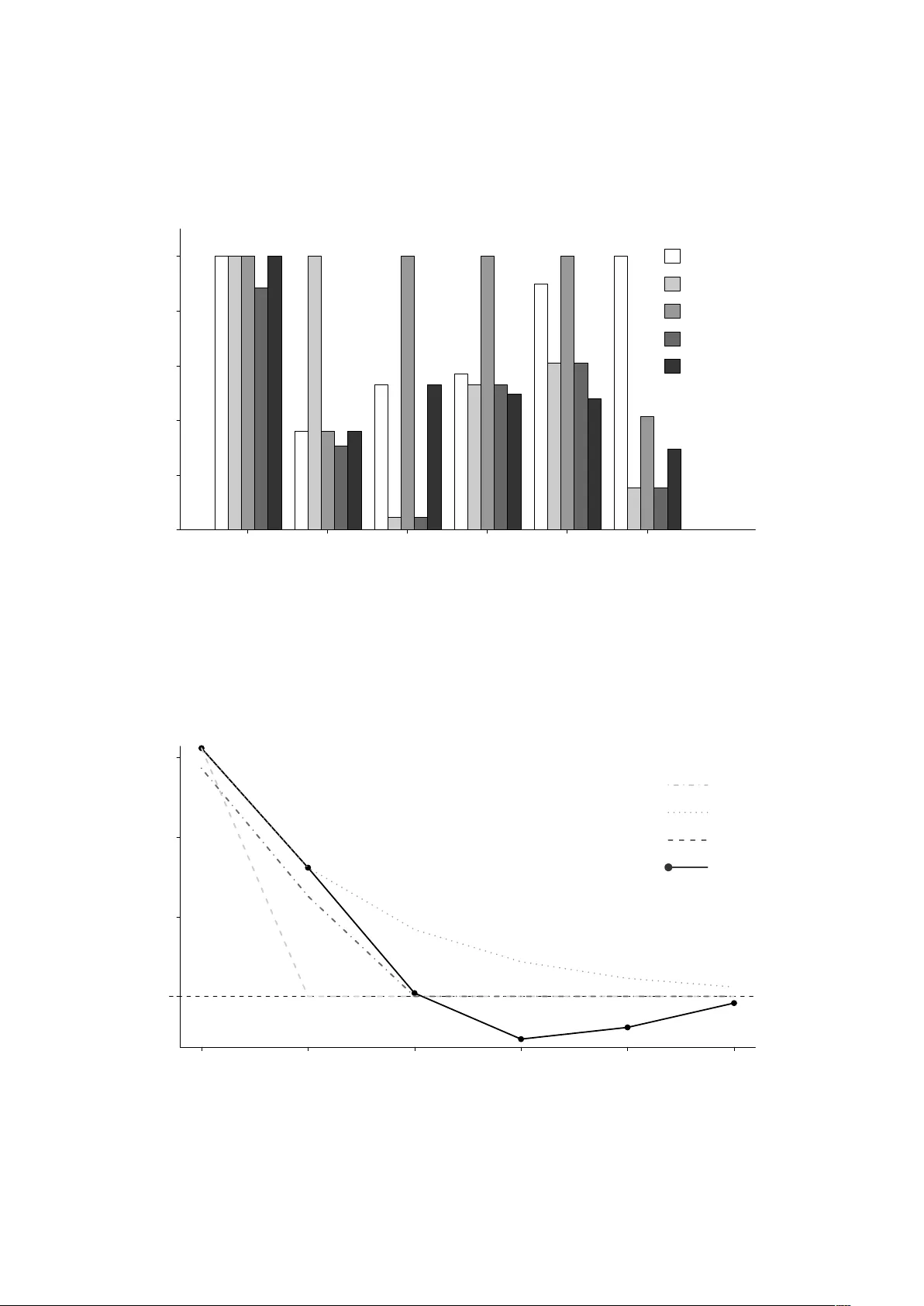
P ARAMETRIC OR NONP ARAMETRIC: THE FIC APPR O A CH F OR ST A TIONAR Y TIME SERIES Gudm und Hermansen, Nils Lid Hjort, Martin Jullum Departmen t of Mathematics, Univ ersit y of Oslo Decem ber 2015 Abstract . W e seek to narrow the gap b et w een parametric and nonparametric mo d- elling of stationary t ime series processes. The approac h is inspired b y recen t adv ances in focused inference and mo del selection tec hniques. The pap er generalises and extends recen t work by developing a new version of the focused information criterion (FIC), di- rectly comparing the performance of parametri c time series models with a nonparametric alternativ e. F or a pre-specified focused parameter, for whic h scrutiny is considered v alu- able, this is ac hiev ed b y comp aring the mean squared error of t he model-based estimators of this quan tit y . In particular, this yields FIC form ulae for co v ariances or correlations at sp ecified lags, for the probability of reaching a threshold, etc. Suitable w eighted av erage v ersions, the AFIC, also lead to model selection strategies for finding the b est model for the purp ose of estimating e.g. a sequence of correlations. Key wor ds: fo cused inference, mo del selection, time series mo delling, risk estimation 1. Intr oduction and summar y The fo cused information criterion (FIC) was introduced in Claesken s & Hjort (2003) and is based on estimating and comparing the accuracy of mo del-based estimators for a c hosen fo cus parameter. This fo cus, say µ , ought to ha v e a clear statistical in terpretation across candidate mo dels. F or a giv en candidate mo del, µ is traditionally expressed as a function of this mo del’s parameters. In general, the fo cus parameter can b e an y sufficien tly smo oth and regular function of the underlying mo del parameters, or more generally its sp ectral distribution. This includes quan tiles, regression co efficien ts, a sp ecified lagged correlation, but also v arious t yp es of predictions and data dep enden t functions, to name some; see Hermansen & Hjort (2015) for a more comp lete list and discussi on of v alid fo cus parameters for time series mo dels. Supp ose there are candidate mo dels M 1 , . . . , M k , leading t o focus parameter estimat es b µ 1 , . . . , b µ k , resp ectiv ely . The underlying idea leading to the FIC is to estimate the mean squared error (mse) of b µ j for each candidate m o del and then select the mo del that ac hiev es Date : December 2015. 1 FIC FOR ST A TIONAR Y TIME SERIES 2 the smallest v alue. The mse in question is mse j = E ( b µ j − µ true ) 2 = bias( b µ j ) 2 + V ar b µ j , comprising the v ariance and the squared bias in relation to the t rue parameter v alue µ true . Th us the FIC consists of finding w ays of assessing, appro ximating and then estimating the mse j for eac h candidate mo del. The winning mo del is the one with smallest d mse j . How this may b e done dep ends on b oth the candidate mo dels and the fo cus parameter, as w ell as on other character istics of the underlying situation. The FIC apparatus hence leads to differen t t yp es of form ulae in different setups; see Claesk ens & Hjort (2008, Ch. 5 & 6) for a fuller discussion and illustrations of suc h criteria for selection among parametric mo dels. Most FIC constructions ha ve b een derived by relying on a suitably defined lo cal missp ecification framework, see again Claesk ens & Hjort (2008, Ch. 5 & 6). In suc h a framew ork the true mo del is assumed to gradually shrink with the sample size, starting from the biggest ‘wide’ mo del and hitting the simplest ‘narro w’ mo del in the limit. In addition, and all candidate mo dels need to lie b etw een these tw o mo del extremes. In the v arious data settings, suc h frameworks t ypically result in squared biases and v ariances of the same asymptotic order, motiv ating certain approximation form ulae for the d mse j in question. In Herman sen & Hjort (2015) suc h a framework is used to derive FIC mac hinery for c ho osing b etw een parametric time series mo dels within broad classes of time series mo dels. See Section 7.5 for some further remarks. The aim of the pr esen t pap er is to deriv e FIC mac hinery whic h will justify comparison and selection among b oth parametric and nonparametric candidate mo dels. The deriv a- tion will b e somewhat different from that of Claesk ens & Hjort (2003) and Hermansen & Hjort (2015) in that w e do not rely on a certain local misspecification framework. W e rather take a more direct approac h follo wing reasoning similar to the developmen t of Jullum & Hjort (2015), where fo cused inference and mo del selection among paramet- ric and nonparametric mo dels are developed for indep enden t observ ations. By including a nonparametric candidate among the parametric mo dels, we will in particular b e able to detect whether our parametric mo dels are off-target. This FIC construction, with a nonparametric alternativ e, therefore has a built-in insurance mech anism against p o orly sp ecified parametric candidates. When one or more parametric models are adequate, suc h are selected as they typically hav e lo wer v ariance. Though our metho ds will b e extended to more general setups later, w e start our de- v elopments with the class of zero-mean stationary Gaussian time series pro cesses. Let { Y t } b e suc h a pro cess. Then the dep endency structure, whic h in such cases deter- mines the en tire mo del, is completely sp ecified by the corresp onding co v ariance function C ( k ) = co v( Y t , Y t + k ), defined for all lags k = 0 , 1 , 2 , . . . . Here w e will, for mathematical FIC FOR ST A TIONAR Y TIME SERIES 3 con venience, w ork with the frequency representation, where the cov ariance function C ( k ) can b e represented by a unique sp ectral distribution G suc h that C ( k ) = Z π − π e ikω d G ( ω ) = 2 Z π 0 cos( k ω ) g ( ω ) d ω , (1.1) pro vided the corresp onding sp ectral distribution G has a con tin uous and symmetric den- sit y g . See among others Brillinger (1975), Priestley (1981) or Dzhaparidze (1986) for a general introduction to time series mo delling in the frequency domain. When necessary , w e will write C g to indicate that this is the cov ariance indexed b y the sp ectral densit y g . Note also that we can obtain the sp ectral density as the F ourier transform of the co v ariance function. The types of parametric mo dels we will consider are typically the classical autore- gressiv e (AR), mo ving av erage (MA) and the mixture (ARMA), all of whic h ha ve clear and w ell defined corresponding sp ectral densities; see e.g. Bro c kwell & Da vis (1991) for an introduction to time series mo delling with such mo dels. Note that the theory dev el- op ed here is general, and that there is nothing other than con v enience that restricts us to these particular classes of parametric mo dels. F or an observ ed series y 1 , . . . , y n , the ra w p eriodogram I n ( ω ) = 1 2 π n     n X t =1 y t exp( iω t )     2 , for − π ≤ ω < π , (1.2) will b e our fav ourite nonparametric model for the underlying sp ectral densit y . The main reason for not considering v ariations of smoothed or tap ered p erio dogram estimators is that we are intere sted in fo cus parameters that inv olv es functions of the in tegrated sp ec- trum, which essentially is a type of smo othing, rendering the pre-smo othing of the raw p eriodogram less critical and often unnecessary . W e will start out considering a class of fo cus functions of the type µ ( G ; h 0 ) = Z π − π h 0 ( ω ) d G ( ω ) , (1.3) where h 0 is a piecewise con tinuous and b ounded function on [ − π , π ], with p oten tially a finite n um b er of jump discontin uities. This class includes e.g. the cov ariance function, whic h is easily seen from (1.1) ab o ve, and allows studying sp ecific parts of the spectral densit y b y using i ndicator functions; see also Gra y (2006) for further illustrations inv olving quan tities of type (1.3). Finding the b est mo del to estimate the in tegrated sp ectrum (or total p o wer/energy) o ver a sp ecific region, ma y b e an int eresting and imp ortan t applications in several areas of research; lik e pharmacology , astronom y , o ceanograph y and in the interpretation of seismic data. The reason is that in all of these situations the observ ed time series is con verted in to the asso ciated sp ectra, where the pro cessed sp ectral densit y and esp ecially FIC FOR ST A TIONAR Y TIME SERIES 4 0.0 0.5 1.0 1.5 2.0 2.5 3.0 0.0 0.5 1.0 1.5 2.0 2.5 ω spectral density true spectral density periodogram Figure 1.1. The true sp ectral density and the raw perio dogram from a simulated au- toregressiv e time series of order 4, with length n = 100 and parameters ρ = (0 . 2 , 0 . 2 , − 0 . 1 , − 0 . 2) and σ = 1 . 30. The shaded regions corresp onds to three differen t fo cus parameters, namely , the integrated spectrum (or total energy) ov er that particular region. the energy ov er certain regions of frequencies, hav e clear in terpretations. F or example, in pharmacology the sp ectrum of EEG/ERP signals may b e used to quan tify certain brain functions, indicating e.g. the effect of a p oten tial drug. In such applications, the differen t mo dels may not alw a ys ha v e clear in terpretations as time series, p er se. The FIC is nev ertheless able to rank the fitted mo dels in terms of estimated precision of estimates, for the fo cus parameter in question. This general idea and particular usage of the FIC is illustrated in Figures 1.1 and 1.2 using sim ulated data from an autoregressiv e mo del of order 4, for fo cus parameters µ j = Z π 0 I ( a j ≤ ω < b j ) g ( ω ) d ω = G ( b j ) − G ( a j ) , for j = 1 , 2 and 3, for the corresp onding in terv als ( a j , b j ) ⊂ [0 , π ); which are mark ed by the shaded regions in Figure 1.1. The candidate mo dels are the autoregressiv e mo dels of order 0–4 and a nonparametric alternative based on integrating the raw p eriodogram (1.2). The AR-mo del of order 0 corresp onds to the indep endence mo del. Here, the FIC w orks well: F or each fo cus parameter it prefers mo dels that all results in estimates that are reasonably close to the true v alue; which in terms if rmse (and absolute deviation from the truth) is not alw ays the nonparametric or true mo del of order 4. Moreo ver, this example also illustrates a second and important concept, namely , that one and the same mo del is not necessarily b est for all fo cus parameters. Note that the FIC prefers an AR(3), AR(4) and AR(1) for the resp ectiv e regions 1, 2, 3. FIC FOR ST A TIONAR Y TIME SERIES 5 0.05 0.10 0.15 0.20 0.25 0.30 0.35 0.05 0.10 0.15 0.20 0.25 0.30 0.35 FIC µ 1 , µ 2 and µ 3 n 0 1 2 3 4 n 0 1 2 3 4 n 0 1 2 3 4 Figure 1.2. The horizon tal lines indicate the true spectral densit y o v er the three shaded regions (of the same colour) shown in Figure 1.1; the three fo cus parameters µ 1 , µ 2 and µ 3 . The corresponding coloured dots sho w the p erformance, in terms of the root of the FIC score for the nonparam teric mo del based on the perio dogram (n) and the autoregressiv e mo dels of order 0–4, where 0 represen t the mo del with indep enden t. A class of fo cus parameters wider than that of (1.3) takes fo cus parameters of the form µ ( G ; h, H ) = H ( µ ( G ; h 1 ) , . . . , µ ( G ; h k )) = H  Z π − π h 1 ( ω ) d G ( ω ) , . . . , Z π − π h k ( ω ) d G ( ω )  , (1.4) for a k -dimensional vector function h ( ω ) = ( h 1 ( ω ) , . . . , h k ( ω )) t , where eac h of the h j is of the ab ov e type, and H ( x 1 , . . . , x k ) a contin uously differentiable function of the x j = µ ( G ; h j ) , j = 1 , . . . , k . The direct correlations corr( Y t , Y t + k ) = co v( Y t , Y t + k ) σ 2 = C ( k ) C (0) = R π 0 cos( k ω ) d G ( ω ) R π 0 d G ( ω ) , for example, are of type (1.4). Another class of estimands captured b y (1.4) are conditional threshold probabilities, sa y P { Y n +1 ≥ y | Y n = y n , . . . , Y n − k = y n − k } , as these are functions of the ( k + 1) × ( k + 1) co v ariance matrix for ( Y n − k , . . . , Y n , Y n +1 ). Later results will allo w us to reac h FIC formulae for this more general class. In Section 2 we pro vide a brief o verview of some standard results needed to obtain go od estimates for v arious mean squared error quant ities. Among other asp ects w e need prop erties of maxim um lik eliho od- or Whittle appro ximated estim ators outside the m o del, and some large-sample results regarding the p erio dogram. Then in Section 3 we motiv ate and dev elop suc h mean squared error estimators, leading to FIC form ulae. In Section 4 w e FIC FOR ST A TIONAR Y TIME SERIES 6 sho w that under certain conditions, a detrended time series ma y b e handled by our FIC sc heme as if it w as the original time series. In Section 5 we extend the FIC metho dology b y deriving an av erage weigh ted fo cused information criterion whic h aims at selecting the b est mo del for estimating a full set of fo cus parameters, p ossibly w eighted to reflect their relativ e imp ortance for the analysis. In Section 6 we discuss certain theoretical b eha vioural asp ects of the derived FIC sc heme, and present the results from a sim ulation study . Some concluding remarks, some of whic h p oin ting to future w ork, are finally pro vided in Secti on 7. 2. Estima tion and appr o xima tions W e start out inv estigating the b eha viour of the t w o most common parametric esti- mation procedures, those based on the maximum likelihoo d method and the asso ciated Whittle approx imation to the log-likeli ho od. W e also giv e some basics for nonparametric mo delling. 2.1. Maxim um likelihoo d estimation outside the mo del. Let y n = ( y 1 , . . . , y n ) t b e a collection of n realisations from a zero mean stationary Gaussian time series pro cess with sp ectral distribution function G and corresp onding sp ectral density g . F urthermore, let the sp ectral distribution function F θ and its corresponding sp ectral densit y f θ = f ( · ; θ ) index an arbitrary parametric candidate mo del, where θ b elongs to some parameter space Θ of dimension say p . The corresp onding full log-lik eliho o d is ℓ n ( θ ) = − n 2 log(2 π ) − 1 2 log | Σ n ( f θ ) | − 1 2 y t n Σ n ( f θ ) − 1 y n , (2.1) where Σ n ( f θ ) is the co v ariance matrix with elemen ts C f θ ( | s − t | ) = 2 Z π 0 cos( ω | s − t | ) f θ ( ω ) d ω for s, t = 1 , . . . , n . Since the class of parametric candidate mo dels is not assumed to necessarily include the true g , the maximum likelihoo d estimator do es not conv erge to a ‘true’ parameter v alue. Instead it con verges to the so-called least false parameter v alue, i.e. e θ n = argmax θ { ℓ n ( θ ) } → p argmin θ { d ( g , f θ ) } = θ 0 , where d ( g , f θ ) = 1 4 π Z π − π n g ( ω ) f θ ( ω ) − 1 − log g ( ω ) f θ ( ω ) o d ω = − 1 4 π Z π − π { log g ( ω ) + 1 } d ω − R ( G, θ ) , (2.2) and where R ( G, θ ) = − 1 4 π Z π − π n log f θ ( ω ) + g ( ω ) f θ ( ω ) o d ω FIC FOR ST A TIONAR Y TIME SERIES 7 ma y b e referred to as the mo del sp ecific part, see e.g. Dahlhaus & W efelmeyer (1996) for details. F urthermore, it can b e sho wn that √ n ( e θ n − θ 0 ) → d J − 1 0 U ∼ N p (0 , J − 1 0 K 0 J − 1 0 ) , where U ∼ N p (0 , K 0 ) , (2.3) with J 0 and K 0 defined b y J 0 = J ( g , f θ 0 ) = 1 4 π Z π − π h ∇ Ψ θ 0 ( ω ) ∇ Ψ θ 0 ( ω ) t g ( ω ) + ∇ 2 Ψ θ 0 ( ω ) { f θ 0 ( ω ) − g ( ω ) } i 1 f θ 0 ( ω ) d ω and K 0 = K ( g , f θ 0 ) = 1 4 π Z π − π ∇ Ψ θ 0 ( ω ) ∇ Ψ θ 0 ( ω ) t n g ( ω ) f θ 0 ( ω ) o 2 d ω , where Ψ θ ( ω ) = log f θ ( ω ). and ∇ Ψ θ ( ω ) and ∇ 2 Ψ θ ( ω ) are resp ectiv ely the vect or of partial deriv ativ es and matrix of second order partial deriv ativ es with resp ect to θ , see Dahlhaus & W efelmey er (1996, Theorem 3.3). Note that J 0 = K 0 under mo del conditions. 2.2. The Whittle appro ximation. The Whittle pseudo-log-lik eliho od is an appro ximation to the full Gaussian log-lik eliho o d ℓ n of (2.1). It was originally suggested b y P . Whittle in the 1950s (cf. Whittle (1953)), and is defined as b ℓ n ( θ ) = − 1 2 n h log(2 π ) + 1 2 π Z π − π log { 2 π f θ ( ω ) } d ω + 1 2 π Z π − π I n ( ω ) f θ ( ω ) d ω i , (2.4) where I n ( ω ) = (2 π n ) − 1 | P t ≤ n y t exp( iω t ) | 2 is the p eriodogram. This approximation is close to the full Gaussian log-likelihoo d in the sense that ℓ n ( θ ) = b ℓ n ( θ ) + O p (1) uni- formly in f , see Coursol & Dacunha-Castelle (1982). More imp ortan t here, ho wev er, is that (2.4) motiv ates an alternativ e estimation pro cedure, namely the Whittle estimator b θ n = argmax θ { b ℓ n ( f θ ) } . This estimator is easier to w ork with in practice (b oth an alytically and n umerically) and shares several prop erties with the maxim um lik eliho o d estimator. In particular √ n ( b θ n − θ 0 ) achiev es the same limit distribution as in (2.3), with the same least false parameter v alue θ 0 as defined in relation to (2.2); see Dahlhaus & W efelmey er (1996) for details. This means that in a large-sample p ersp ectiv e, the maxim um like- liho od estimator and the simpler Whittle estimator are equally efficient and essentia lly in terchangeable. 2.3. Nonparametric mo delling. As mentioned in the introduction, w e shall use the p eri- o dogram in (1.2) for nonparametric mo delling. Under appropriate short memory condi- tions, it follo ws from Brillinger (1975, Theorem 5.5.2) that E { I n ( ω ) } = g ( ω ) + O ( n − 1 ), i.e. that the p eriodogram is asymptotically un biased as an estimator of the sp ectral den- sit y . W e shall th us use b G n ( ω ) = Z ω − π I n ( u ) d u, (2.5) FIC FOR ST A TIONAR Y TIME SERIES 8 as a canonical estimator for the sp ectral distribution G ; for whic h √ n ( b G n ( ω ) − G ( ω )) → d N  0 , 4 π Z ω − π g ( u ) 2 d u  , see e.g. T aniguc hi (1980). 3. P arametric versus nonp arametric W e shall no w obtain large-sample appro ximations for the fo cus parameter estimators. These shall then b e used to construct approxi mate mse formulae for each mo del’s estimator of the fo cus parameter. When estimated these mses then giv e the FIC formula e. 3.1. Ho w to compare parametric and nonparametric mo dels? In completely general terms, let µ ( G ) b e a fo cus function, i.e. a functional mapping of the sp ectral distribu- tion G to a scalar v alue. This ma y b e estimated parametrically b y estimators of the form b µ pm = µ ( F b θ n ), or nonparametrically by b µ np = µ ( b G n ). Other estimators of θ and G may also b e used, ho wev er. T ypically , the collection of parametric candidate mo dels do es not include the true G . The question is then which mo del should w e use – parametric or nonparametric – for estimating the fo cus parameter. Assume for the nonparametric and eac h of the parametric candidate mo dels that √ n ( b µ np − µ true ) → d N(0 , v np ) and √ n ( b µ pm − µ 0 ) → d N(0 , v pm ) , where µ true = µ ( G ) is the true v alue of the fo cus parameter and µ 0 = µ ( F θ 0 ) is the fo cus function ev aluated under the least false parametric mo del F θ 0 as discussed in relation to (2.2). Then, without going into details, the large-sample results ab o ve motiv ate the follo wing first-order appro ximations for the mse of the estimated fo cus parameters: mse np = 0 2 + v np /n = v np /n and mse pm = b 2 + v pm /n, (3.1) where b = µ 0 − µ true . The remainder of this section will b e used to motiv ate and obtain go od estimators for the mean squared errors in (3.1) with the class of fo cus param ters of the form µ ( G ; h 0 ) defined in (1.3), and the more general µ ( G ; h, H ) in (1.4). 3.2. Deriving un biased risk estimates. In the deriv ation b elo w, the parametric candidates F θ will b e fitted using the Whittle estimator b θ n as defined in (2.4), while w e will use the canonical p erio dogoram based estimator in (2.5) for nonparametric estimation of the sp ectral distribution G . Using the Whittle estimator in collab oration with (2.5) results in a con v enien t sim plifi- cation of the deriv ations b elo w; extending the argumen ts to full ML estimation is relativel y straigh tforward, using techniques in Dahlhaus & W efelmeyer (1996). This motiv ates the FIC FOR ST A TIONAR Y TIME SERIES 9 follo wing nonparametric and parametric estimators for fo cus parameters µ ( G ; h 0 ) on the form of (1.3): b µ np = Z π − π h 0 ( ω ) I n ( ω ) d ω = 1 n y t n Σ n ( h 0 ) y n and b µ pm = Z π − π h 0 ( ω ) f b θ n ( ω ) d ω , where Σ n ( h 0 ) is a n × n -dimensional symmetric T o eplitz matrix, having elemen ts of the general form σ n,s,t ( h 0 ) = Z π − π cos( ω | s − t | ) h 0 ( ω ) d ω . for s, t = 1 , . . . , n . The following proposition establishes the join t limit distribution for the estimators ab o v e (suitably normalised), which in turn will b e used to obtain go o d appro ximations for their resp ectiv e mean squared errors. Prop osition 1. Let y 1 , . . . , y n b e realisations from a stationary Gaussian time series mo del with sp ectral densit y g assumed to b e uniformly b ounded a wa y from b oth zero and infinit y . Supp ose | h 0 | is b ounded in ω , that f θ is t wo t imes differen tiable with respect to θ , and that f θ and these deriv atives, ∇ f θ and ∇ 2 f θ , are con tinuous and uniformly b ounded in b oth ω and θ in a neighbourho o d of the least false parameter v alue θ 0 as defined in (2.2) ab o ve. Then √ n ( b µ np − µ true ) √ n ( b µ pm − µ 0 ) ! → d X 0 c t 0 J ( g , f θ 0 ) − 1 U ! ∼ N 2 0 0 ! , v np v c v c v pm !! , (3.2) where v np = 4 π Z π − π { h 0 ( ω ) g ( ω ) } 2 d ω and v pm = c t 0 J ( g , f θ 0 ) − 1 K ( g , f θ 0 ) J ( g , f θ 0 ) − 1 c 0 , with J and K as defined b elo w (2.3), and v c = c t 0 J ( g , f θ 0 ) − 1 d 0 , where the c 0 is the partial deriv ativ e of µ ( F θ 0 ; h ) with resp ect to θ , i.e. c 0 = ∇ µ ( F θ 0 ; h ) = R π − π h 0 ( ω ) ∇ f θ 0 ( ω ) d ω and d 0 = co v( X , U ) = Z π − π ∇ f θ 0 ( ω ) h 0 ( ω ) g ( ω ) 2 f θ 0 ( ω ) 2 d ω . Pr o of. It follo ws from the results in (Dzhaparidze, 1986, Ch. 2) that b θ n − θ 0 = J ( g , f θ 0 ) − 1 U n + o p (1 / √ n ), where U n = ∇ b ℓ n ( f θ 0 ) and U n = − 1 2 { T r(Σ n ( ∇ Ψ θ 0 )) − y t n Σ n ( ∇ Ψ θ 0 /f θ 0 ) y n } , where Ψ θ 0 = log f θ 0 and ∇ Ψ θ 0 is the v ector of its partial deriv ativ es. As a conse- quence, a T a ylor expansion motiv ated b y the standard delta metho d giv es b µ pm − µ 0 = c t 0 J ( g , f θ 0 ) − 1 U n + o p (1 / √ n ). Since √ nU n → d U b y the assumptions of the prop osition (Dzhaparidze, 1986), the parametric part of the result holds. In addition X n = ( b µ np − µ true ) = 1 n y t n Σ n ( h 0 ) y n − µ true , FIC FOR ST A TIONAR Y TIME SERIES 10 whic h can b e shown, by a mo dified v ersion of the argumen t leading to the limit distribution of U n , t o hav e the prop ert y that √ nX n → d X 0 ∼ N(0 , v np ). This pro v es the nonparametric part of the result. W e finally need to sho w that these conv ergence results hold joint ly . Since the tw o driv ers in the deriv ation of the limit distribution, y t n Σ n ( h 0 ) y n /n and U n , are quadratic forms, the join t limit distribution is readily obtainable by a Cram ´ er–W old t yp e of argumen t. T o see how, let a be a vector in R 2 to b e used in the Cram ´ er– W old argumen t, and define Λ n = a 1 √ nX n + a 2 √ nU n = 1 √ n y t n Σ n ( a 1 h 0 + a 2 ∇ Ψ θ 0 /f θ 0 ) y n + γ n where γ n = √ n { a 1 µ true − a 2 T r(Σ n ( ∇ Ψ θ 0 )) / 2 } . The γ n cancels out the mean, here, such that Λ n has mean zero. This is once again just a quadratic form, hence, Λ n is normal under the assumptions of the prop osition; see Dzhaparidze (1986) or Hermansen & Hjort (2014b) for deriv ations of a similar t yp e. The pro of is completed by observing that by Dahlhaus & W efelmey er (1996, Lemma A.5), the cov ariances take the relev an t form co v( X n , U n ) = 2 n T r { Σ n ( h 0 )Σ n ( g )Σ n ( ∇ Ψ θ /f θ )Σ n ( g ) } → Z π − π ∇ f θ 0 ( ω ) h 0 ( ω ) g ( ω ) 2 f θ 0 ( ω ) 2 d ω . □ W e next extend the ab ov e prop osition to the more general class of W e next extend the ab o v e proposition to the more general class of focus parameters µ ( G ; h, H ) in (1.4), b eing a contin uously differen tiable function of a finite num b er of the µ ( G ; h 0 ) functions. The nonparametric and parametric estimators for this class take the form b µ np = H  n − 1 y t n Σ n ( h 1 ) y n , . . . , n − 1 y t n Σ n ( h k ) y n  and b µ pm = H  Z π − π h 1 ( ω ) f ( ω ; b θ n ) d ω , . . . , Z π − π h k ( ω ) f ( ω ; b θ n ) d ω  . Prop osition 2. Under the conditions of Proposition 1 the fo cus parameters µ ( G ; h, H ) in (1.4), with estimators and estimands as ab o ve, fulfils √ n ( b µ np − µ true ) √ n ( b µ pm − µ 0 ) ! → d ∇ H np X ∇ H pm c t J ( g , f θ 0 ) − 1 U ! ∼ N 2 0 0 ! , v np v c v c v pm !! , (3.3) where v np = ∇ H np { 4 π Z π − π { h ( ω ) g ( ω ) } 2 d ω }∇ H t np and v pm = ∇ H pm c t J ( g , f θ 0 ) − 1 K ( g , f θ 0 ) J ( g , f θ 0 ) − 1 c ∇ H t pm , and v c = ∇ H pm c t J ( g , f θ 0 ) − 1 d ∇ H t np , where ∇ H np and ∇ H pm are the gradien ts of H ev aluated at resp ectiv ely ( µ ( G ; h 1 ) , . . . , µ ( G ; h k )) and ( µ ( F θ 0 ; h 1 ) , . . . , µ ( F θ 0 ; h k )) , c is the FIC FOR ST A TIONAR Y TIME SERIES 11 k × p -dimensional matrix with rows given by ∇ µ ( F θ 0 ; h j ) , j = 1 , . . . , k and d = cov( X , U ) = Z π − π ∇ f θ 0 ( ω ) h ( ω ) g ( ω ) 2 f θ 0 ( ω ) 2 d ω . Pr o of. By Prop ostion 1, we see that (3.2) holds for eac h µ ( G ; h j ). Let no w X n,j = 1 n y t n Σ n ( h j ) y n − µ true for j = 1 , . . . , k . By extending the Cram ´ er–W old argumen t in Pro- p ostion 1 to all of X n, 1 , . . . , X n,k , U n , w e see that there is joint conv ergence for all these. The standard (multiv ariate) delta metho d then completes the pro of. □ Remark 1. F rom the underlying structure of the pro of of Prop ositions 1 and 2, and the arguments (of e.g. Dahlhaus & W efelmey er (1996) or Dzhaparidze (1986)) used to sho w that the Whittle estimator has the same large-sample prop erties as the maximu m lik eliho o d estimator, it is clear that the conclusions of the t wo prop ositions sta ys true if w e replace Whittle with full maxim um lik eliho o d estimation. The nonparametric estimator is b y construction unbiased in the limit; an estimate for the risk is therefore easily obtained from the v ariance formula ab o ve. F or the parametric candidate, w e need in addition an un biased estimate for the squared bias. F ollo wing Jullum & Hjort (2015) w e start with b b = b µ pm − b µ np as an initial estimate for b = µ 0 − µ true . Since it follows from (3.2) that √ n ( b b − b ) → d c t J − 1 U − X ∼ N(0 , κ ), where κ = v pm + v np − 2 v c , w e hav e E b b 2 ≈ b 2 + κ/n + o (1 /n ). This leads to mse estimators of the form FIC np = d mse np = b v np /n, FIC pm = d mse pm = d bsq + b v pm /n = max(0 , b b 2 − b κ/n ) + b v pm /n. (3.4) F or the most general fo cus parameter form ulation in (1.4), the v ariance and co v ariance estimators take the form b v np = ∇ b H np { 2 π Z π − π h ( ω ) 2 I n ( ω ) 2 d ω }∇ b H t np , and b v pm = ∇ b H pm b c t J ( I n , f b θ n ) − 1 K ( I n / √ 2 , f b θ n ) J ( I n , f b θ n ) − 1 b c ∇ b H pm , where b c = ( ∇ µ ( F b θ n ; h k ) , . . . , ∇ µ ( F b θ n ; h k )) t , ∇ b H np and ∇ b H pm are the gradients of H ev alu- ated at resp ectiv ely ( µ ( b G n ; h 1 ) , . . . , µ ( b G n ; h k )) and ( µ ( F b θ n ; h 1 ) , . . . , µ ( F b θ n ; h k )), and J and K are as defined in relation to (2 . 3) – using I n ( w ) 2 / 2 as the canonical nonparametric un biased estimator for g ( w ) 2 . These are all consisten t according to T aniguchi (1980); Deo & Chen (2000). With FIC scores as ab o ve, represen ting clear-cut estimates of the risk of the nonpara- metric and parametric mo dels’ estimators of µ , our mo del selection strategy turns out as follo ws: Compute the FIC score for each candidate model, rank them accordingly , and select the mo del and estimator asso ciated with the smallest FIC score. The same FIC pm FIC FOR ST A TIONAR Y TIME SERIES 12 form ula (with different estimates and quantities) is used for all of the p ossibly m different parametric candidate mo dels for simul taneous selection among the m + 1 mo dels. This is p erfectly fine as the FIC pm form ula do es not dep end on the other parametric mo dels. Although w e ha v e concen trated on fo cus functions µ ( G ; h ) and µ ( G ; h, H ) given by (1.3-1.4), our fo cused mo del selection strategy applies also to more general fo cus parame- ters, as long as join t limit distributions lik e (3.2) and (3.3) ma y b e pro v en. In completely general terms, our results ma y b e generalised to fo cus parameters of the form µ = T ( G ) for well-beha v ed functionals T mapping the sp ectral distribution G to a scalar v alue. The t yp e of smo othness required for T is in fact that the functional is so-called Hadamard dif- feren tiable at G and F θ 0 , see e.g. v an der V aart (2000, Theorem 20.8) for further details. This allo ws us, for instance, to handle fo cus parameters in v olving quan tiles of the sp ectral distribution G . It is also p ossible to extend the arguments to other parametric estima- tion pro cedures, esp ecially if they are deriv ed as minimisers of the empirical analogue of argmin { R ( G, θ ) } for R the mo del sp ecific part of p ossibly differen t div ergence measure than in (2.2), see Dahlhaus & W efelmeye r (1996) and T aniguc hi (1980) for alternativ es. 4. Models with trends So far w e ha v e only considered stationary time series with mean zero. In real appli- cations, this is often an unrealistic assumption to make. Even if the series is stationary , the underlying mean is rarely exactly zero; the common solution in suc h cases is to de- trend the series. In time series mo delling, detrending usually refers to the act of removing an estimated or deterministic trend from the observ ed series b efore the main analysis. This may b e a complex function of time and cov ariates including seasonal effects, or b e as simple as subtracting the arithmetic mean. A common approac h is to work with the detrended series, which we will denote b y b y t , and then analyse this series using mo dels for stationary time series, without factoring in the extra estimation uncertain t y in v olved in the detrending. This is often unproblematic, but even the inno cen t action of subtract- ing the mean ma y hav e unforeseen consequences (t ypically for the so-called second order prop erties). Hermansen & Hjort (2014b) sho ws that such a simple op eration alter the underlying motiv ation and in terpretation of the AIC for stationary Gaussian time series. Th us, sp ecial care is required for suc h an op eration. Supp ose the observed series is generated b y the mo del Y t = m ( x t , β ) + ε t , (4.1) where the x t are p -dimensional co v ariates, the m is of known parametric structure, and { ε t } is a zero mean stationary Gaussian time series pro cess with sp ectral distribution function G and corresp onding density g . Assume further that w e are able to estimate β b y a suitable b β n with reasonable precision. The question is then whether the results of FIC FOR ST A TIONAR Y TIME SERIES 13 Section 3 are still v alid also with detrended data, suc h that w e ma y still use the same FIC form ulae. Prop osition 3. Supp ose the sp ectral densities g and f θ and function h satisfy the conditions of Prop osition 1, and that the assumed trend m and corresponding estimator b β for the unknown β are such that √ n ( b β n − β ) = O p (1) . Assume further that in a neigh b ourho o d of β we hav e m ( x, b β n ) = m ( x, β ) + ∇ m ( x, β ) t ( b β n − β ) + r n ( x ) , with max i | r n ( x i ) | = o p (1 / √ n ) and |∇ m ( x, β ) | b ounded in x . Then the conclusions of Prop osition 1 are still true if w e replace y t with the detrended b y t = y t − m ( x t , b β n ) . Pr o of. W e will sho w that the result follo ws as a corollary from certain general results regarding limit b eha viour of quadratic forms from Hermansen & Hjort (2014a, Section 3). The argumen t is structured similarly to that of Prop osition 1 and is built around a Cram ´ er–W old type of argumen t. Observe that if w e replace y t with the detrended b y t = y t − m ( x t , b β n ), w e now hav e b X n = ( b y t n Σ n ( h 0 ) b y n − µ true ) and similarly b U n = − 1 2 { T r(Σ n ( ∇ Ψ θ 0 )) − b y t n Σ n ( ∇ Ψ θ 0 /f θ 0 ) b y n } , where b y n = ( b y 1 , . . . , b y n ) t . Again, for an y a = ( a 1 , a 2 ) in R 2 , w e now hav e b Λ n = a 1 √ n b X n + a 2 √ n b U n = b y t n Σ n ( a 1 h 0 + a 2 ∇ Ψ θ 0 /f θ 0 ) b y n / √ n + γ n , with γ n as in the pro of of Proposition 1. Then, according to Proposition 3.1 of Herman sen & Hjort (2014a), b Λ n − Λ n = o p ( n − 1 / 2 ) where Λ n = ε t n Σ n ( a 1 h 0 + a 2 ∇ Ψ θ 0 /f θ 0 ) ε n / √ n + γ n , where ε n = ( ε 1 , . . . , ε n ) t has elements corresp onding to (4.1). Since the limit b eha viour of Λ n is what defines the limit distribu- tion in Proposition 1, the argumen t is essen tially complete. □ The ab o ve prop osition ma y also b e extended to the fo cus parameter in (1.4), as handled in Proposition 2. T raditionally , the least squares estimator has been the canonical metho d for estimating β in mo dels of the form of (4.1). As an illustration, consider the linear regression mo del with dep enden t errors where Y t = x t t β + ε t , for p -dimensional co v ariates x t , and where { ε t } is a zero mean stationary Gaussian time series pro cess with sp ectral density g . On matrix form this yields y n = X β + ε n , where X is the related n × p -dimensional design matrix. The ordinary least squares estimate for β is then giv en b y b β n = ( X t X ) − 1 X t y n . Then, in order for b β n to satisfy the conditions of Prop osition 3, it is sufficien t that n V ar( b β n ) = n ( X t X ) − 1 X t Σ n ( g ) X ( X t X ) − 1 = o (1), whic h is clearly satisfied if X t X/n → p Q 1 and X t Σ( g ) X/n → p Q 2 , as n approach es infinit y , where Q 1 and Q 2 are b oth finite p ositiv e definite matrices. These are the standard assumptions FIC FOR ST A TIONAR Y TIME SERIES 14 needed to ensure consistency of b oth standard and generalised least squares for mo dels with correlated errors. 5. A vera ge f ocused informa tion criterion W e ha ve so far concentr ated on inference for a single fo cus parameter µ . A natural generalisation of this is to consider several fo cus parameters joinly , say correlations of orders 1 to 5. The FIC mac hinery can easily b e lifted to such a situation, inv olving a w eigh ted a verage of FIC scores, the AFIC, with w eights reflecting imp ortance dictated b y the statistician. Supp ose in general terms that estimands µ ( u ) are under consideration, for u in some index set. F or eac h of th ese w e h a v e the nonparametric b µ np ( u ) and on e o r m ore parametric estimators b µ pm ( u ). These ty pically ha v e v ersions of Prop ositions 1 or 2, leading as p er (3.1) to mse np ( u ) = 0 2 + v np ( u ) and mse pm ( u ) = b ( u ) 2 + v pm ( u ) , with b ( u ) = µ 0 ( u ) − µ true ( u ). These mean squared errors can then b e com bined, via some suitable cumulativ e wei gh t function W ( u ), to risk np = Z v np ( u ) d W ( u ) and risk pm = Z { b ( u ) 2 + v pm ( u ) } d W ( u ) Here d W ( · ) is meant to reflect the relative imp ortance of the differen t µ ( u ), and should stem from the statistician’s judgemen t and the actual context. Based on the data we ma y no w form the following natural estimates of these risk quantities: AFIC np = Z b v pm ( u ) d W ( u ) , AFIC pm = Z  max { b b ( u ) 2 − b κ ( u ) /n } + b v pm ( u )  d W ( u ) . (5.1) This operation also needs the cov ariances v c ( u ), as b κ ( u ) is to b e con structed as the natural estimator of κ ( u ) = v pm ( u ) + v pm ( u ) − 2 v c ( u ). The AFIC scheme (5.1) can b e used in a v ariety of circumstances. A t ypical appli- cation may in v olve assessing mo dels for estimating a threshold probabilit y P { Y n +1 ≥ a } o ver a set of man y a , again with a w eigh t function w ( a ) indicating relativ e imp ortance. Another attractiv e application is for the task of estimating correlations corr( h ) for lags h = 1 , 2 , 3 , . . . , p erhaps with a decreasing w ( h ). The AFIC metho d ma y similarly b e applied for comparing the p opular autorcorrelation function, such as acf in the statisti- cal soft ware pack age R (R Core T eam, 2015), with p oten tially more accurate parametric alternativ es. FIC FOR ST A TIONAR Y TIME SERIES 15 6. Perf ormance In the presen t section we will discuss some b eha vioural asp ects of the deriv ed FIC metho dology . First we presen t some theoretical consequences of using our new FIC con- struction for mo del selection. Then we discuss some issues related to the more practical p erformance of this criterion, and illustrate some of these in a simulati on study . The goal is not to conduct a broad simulati on based in v estigation, but rather show the p otent ial of ha ving a criterion for selecting among parametric mo dels and a nonparam etric alternativ e in a simple pro of of concept t yp e of illustration. 6.1. FIC under mo del conditions. Although we hav e b een w orking outside sp ecific para- metric mo del c onditions when deriving the FIC (and AFIC) abov e, it is natural to ask ho w the criteria selects when a parametric mo del is indeed correct. Consider how ev er first the case where a sp ecific parametric candidate mo del is incorrect and hav e bias b  = 0. F rom the structur e of the FIC formulae in (3.4) and the consistency of the in volv ed v ariance and co v ariance estimators, w e see that FIC np = o p (1), while FIC pm = O p (1) + o p (1) = O p (1). I.e. the squared bias term dominates completely , and the probabilit y that the FIC will select this particular parametric mo del will tend to 0 as n → ∞ . If all the paramet- ric candidate mo dels are biased in this sense, then the FIC will even tually prefer the nonparametric mo del when the sample size increases. Going more in to detail, it is seen from the FIC formulae in (3.4) that the FIC prefers a sp ecific parametric mo del ov er the nonparametric whenev er max( b b 2 − b κ/n, 0) + n − 1 b v pm ≤ n − 1 b v np . Whenev er b v np ≥ b v pm , this is seen to b e equiv alen t to Z n ≤ 2 , where Z n = ( n b b 2 ) / ( b v np − b v c ). It turns out that under mo del conditions, w e ha v e v c = v pm . This is rather straigh tfor- w ard to see by in vestigating the forms of v c and v pm in volv ed in Prop osition 2, in addition to the forms of K 0 and J 0 . Inserting g = f θ 0 in these form ulae rev eals that K 0 = J 0 , ∇ H np = ∇ H pm and c = d and thereb y v c = v pm . No w, due to the consistency , w e hav e b v np − b v c → p v np − v pm . F urther, the limit distribution result of √ n ( b b − b ) giv en ab o v e (3.4) ensures that Z n → d χ 2 1 , with χ 2 1 a c hi-squared distributed v ariable with o ne degree of freedom. That is, the limiting probabilit y that the parametric mo del will b e selected ov er the nonparametric when it is indeed true is P { Z n ≤ 2 } → P { χ 2 1 ≤ 2 } ≈ 0 . 843. Thus, if one of the parametric candidate mo dels is correct, and the others hav e biases b  = 0, then, for sufficiently large samples, the first parametric mo del and estimator will b e selected FIC FOR ST A TIONAR Y TIME SERIES 16 with a probability tending to 84.3%, while the nonparametric will b e selected in the other 15.7% proportion. k relativ e root − mean − squared error 0.0 0.2 0.4 0.6 0.8 1.0 0 1 2 3 4 5 nonparametric AR(0) AR(1) MA(1) AR(2) Figure 6.1. Relative ro ot-mse for each candidate mo del fitted to the six fo cus parame- ters µ k = C ( k ), for k = 0 , . . . , 5. The ro ot-mse is computed based on 5000 sim ulated AR(2) series of length n = 100, with σ = 1 . 0 and ρ = (0 . 7 , − 0 . 6), F or ease of comparison we hav e scaled the ro ot-mse to the unit interv al. 0 1 2 3 4 5 0.0 0.5 1.0 1.5 least false cov ariance functions k C(k) AR(0) AR(1) MA(1) AR(2) Figure 6.2. The fiv e least false co v ariance functions under the assumption that the true mo del is an autoregressive mo del sp ecified by the parameters σ = 1 . 0 and ρ = (0 . 7 , − 0 . 6). FIC FOR ST A TIONAR Y TIME SERIES 17 6.2. FIC in practice. Figure 6.1 sho ws the relativ e ro ot-mse for estimating the fo cus parameter µ k = µ ( G ; h k ) = Z π − π cos( ω k ) g ( ω ) d ω = C g ( k ) , for k = 1 , . . . , 5 , (6.1) based on the following fiv e candidates mo dels: the indep endence mo del (autoregressiv e of order zero); the autoregressiv e of orders one and tw o; the mo ving a verage of order one; and finally the nonparametric one, where nothing more is assumed than saying that the series is stationary with a finite v ariance. The true mo del is an autoregressiv e mo del sp ecified b y the parameters ρ = (0 . 7 , − 0 . 6) and σ = 1 . 0. This means that all but t w o, the autoregressiv e mo del of order tw o and the nonparametric mo del, are missp ecified. The corresp onding least false cov ariance estimates are plotted in Figure 6.2. In the sim ulation study , w e hav e used B = 5000 rep etitions of length n = 100 to compute the actual relativ e ro ot-mse v alues for eac h candidate. Note that since w e hav e included the true mo del among our candidates, nonparametric estimation is never the optimal choice; it is ho wev er often close and it is the second b est choice for lags 1 and 3. F or lags 2 and 5, where the true v alues are close to zero, the simpler mo dels, like AR(0) and MA(1), are highly successful, achieving reasonably lo w bias and also low v ariance. Figure 6.3. The prop ortion for which the different criteria selects the model with the theoretical lo west ro ot-mean-squared error. The model-selectors ar e alw ays nonparametric, FIC, AIC and BIC. The results are based on 5000 simulated series. In Figure 6.3 and 6.4 w e further inv estigate the p erformance of the FIC. Here, w e compare our FIC mac hinery with three other mo del selection strategies, (i) to alwa ys use FIC FOR ST A TIONAR Y TIME SERIES 18 the nonparametric mo del, (ii) select the b est parametric mo del according to the AIC and (iii) the parametric mo del selected by the BIC. Note that the AIC and BIC to ols do not w ork for the nonparametric mo del, since there is no lik eliho o d function. In Figure 6.3 we ha ve counted ho w many times eac h criterion selects the mo del that obtains the smallest ro ot-mse v alue, for each fo cus parameter µ k as defined in (6.1). Figure 6.4 con tains the corresp onding attained ro ot-mse v alues. Note that for lag 1 the theoretical ro ot-mse for the autoregressiv e mo dels are, for all practical purp oses, equal to that obtained by the nonparametric mo del. In all other cases, the nonparametric mo del has a ro ot-mse larger than the optimal mo del. In this il lustration, the FIC behav es more or less as in tended, b y selecting (on a v erage) the mo dels that pro duces the smallest risk. The amount of evidence is b y no means conclusiv e, but it indicates that the FIC mac hinery has a real p oten tial. Figure 6.4. The relativ e ro ot-mean-squared (computed in the same sim ulations) for the mo dels selected by FIC, AIC and BIC, and b y alw ays using the non- parametric mo del. 7. Concluding remarks Here we offer a list of conclucing comments, some pointin g to further relev ant research. 7.1. Mo del a v eraging. The FIC scores ma y also b e used to combine the most promising estimators in to a mo del av eraged estimator, say b µ ∗ = P j c ( M j ) b µ j , with c ( M j ) given higher v alues for mo dels M j with higher FIC scores; as discussed in Hjort & Claeskens (2003). FIC FOR ST A TIONAR Y TIME SERIES 19 7.2. The conditional FIC. F or time series pro cesses, sev eral interesting and imp ortan t fo cus parameters are naturally related to predictions, are sample size dep enden t or other- wise form ulated conditional on past observ ations. The classical example is k -step ahead predictions. A class of such estimands could tak e the form µ ( α, γ , y 1 , . . . , y m ) = P { Y n +1 > α and Y n +2 > γ | y 1 , . . . , y m } for a suitable choice of α . The dep endency on previous data requires a new and ex- tended mo delling framew ork, whic h in Hermansen & Hjort (2015, Sections 5 & 6) led to generalisations and also motiv ated a conditional fo cused information criterion (cFIC). In completing the FIC-framew ork for selecting among parametric and nonparametric time series mo dels, such considerations should also b e tak en in to account. 7.3. Linear time series pro cesses. Building on W alk er (1964); Hannan (1973); Brillinger (1975), the main results of Section 3 can b e extended to more general t yp es of time series pro cesses, lik e the generalised linear pro cesses (cf. Priestley (1981)); also without the assumption of Gaussian innov ation terms. 7.4. T rends and cov ariates. In the presented wor k, our fo cus was on the dep endency structure only . Ho wev er, the metho ds and results of our pap er ma y b e generalised to select sim ultaneously among mo dels with different trends and dep endency structures, like Y t = m ( x t , β ) + ε t , with ε t a stationary Gaussian time pro cess. These issues, leading to a larger rep ertoire of FIC formulae, will b e returned to in later w ork. Since it is generally hard to estimate b oth the trend and dep endency structure using a full nonparametric framew ork, the tw o main c hallenges is to extend the existing w ork to handle the case with v arious parametric candidates for the trend m ( x t , β ) and b oth parametric mo dels and a nonparametric candidate for the dep endency , i.e. the sp ectral distribution (since w e are w orking under the Gaussian assumption). Alternativ ely , w e ma y assume that the ε t b elongs to an appropriate width family of parametric stationary time ser ies pro cesses, suc h as the autoregressive AR, the moving av erage MA or the mixture ARMA (cf. Bro c kw ell & Da vis (1991)) and instead compare a nonparametric metho d for estimating the trend part of the mo del, p erhaps extending this to functions of the t yp e m ( t, x i , β ), against a class of parametric alternatives. 7.5. The lo cal large-sample framework. As men tioned in the int ro duction, Hermansen & Hjort (2015) derives FIC for selecting among parametric time series mo dels using a lo cal asymptotics framework. The parametric candidate mo dels then hav e sp ectral densities b elonging to a parametric family f ( · ; θ , γ ), with a p -dimensional protected θ and a q - dimensional op en γ . This constitutes a set of 2 q p oten tial parametric candidate mo dels. The full (or wide) mo del is represented b y the sp ectral densit y f ( · ; θ , γ ). At the other end of the sp ectrum, the narrow mo del corresp onds to fixating γ = γ 0 , a known v alue, with the FIC FOR ST A TIONAR Y TIME SERIES 20 resulting f ( · ; θ ) = f ( · ; θ , γ 0 ). The lo cal missp ecification framew ork then assumes that the true spectral densit y tak es the form f ( · ; θ 0 , γ 0 + δ / √ n ), for some unkno wn q -dimensional δ describing the distance to the wide mo del. This framew ork causes v ariances and squared biases to b ecome of the same order of magnitude O (1 /n ). Those lead to approxim ation form ulae for the mean squared error and FIC formulae for nested parametric mo dels, whic h are different from those obtained in this pap er. The introduction of the ‘asymptotically correct’ nonparametric mo del of the present pap er allo wed us to deriv e FIC formulae ev en when sidestepping the ab o v e lo cal misspeci- fication assump tion. An alternativ e approac h is to retain the local asymptotics framew ork and work with sp ectral densities of the t ype f r ( ω ) = f θ 0 ( ω ) + r ( ω ) / √ n , where f θ 0 is a standard type of parametric mo del. Suc h structures ha v e already b een work ed with in Dzhaparidze (1986), making the extension p oten tially less cumbersome. This will not b e dealt with here, how ever. References Brillinger, D. (1975). Time Series: Data Analysis and The ory . Holt, Rinehart and Winston. Br ockwell, P. & Da vis, R. (1991). Time Series: The ory and Metho ds . Springer. Claeskens, G. & Hjor t, N. L. (2003). The fo cused information criterion [with dis- cussion and a rejoinder]. Journal of the Americ an Statistic al Asso ciation 98 , 900–916. Claeskens, G. & Hjor t, N. L. (2008). Mo del Sele ction and Mo del Aver aging . Cam- bridge: Cam bridge Universit y Press. Coursol, J. & Da cunha-Castelle, D. (1982). Remarks on the appro ximation of the lik eliho od function of a stationary Gaussian pro cess. The ory of Pr ob ability and its Applic ations 27 , 162–167. D ahlhaus, R. & Wefelmeyer, W. (1996). Asymptotically optimal estimation in missp ecified time series mo dels. Annals of Statistics 24 , 952–973. Deo, R. S. & Chen, W. W. (2000). On the integra l of the squared p erio dogram. Sto chastic pr o c esses and their applic ations 85 , 159–176. Dzhap aridze, K. (1986). Par ameter Estimation and Hyp othesis T esting in Sp e ctr al A nalysis of Stationary Time Series . Berlin: Springer. Gra y, R. (2006). T o eplitz and Cir culant Matric es: A R eview . No w publishers Inc. Hannan, E. J. (1973). The asymptotic theory of linear time-series mo dels. Journal of Applie d Pr ob ability 10 , 130–145. Hermansen, G. & Hjor t, N. L. (2014a). Limiting normality of quadratic forms with applications to time series analysis. T ec h. rep., Univ ersit y of Oslo and Norw egian Computing Centre. FIC FOR ST A TIONAR Y TIME SERIES 21 Hermansen, G. & Hjor t, N. L. (2014b). A new approach to Ak aike’s information criterion and mo del selection issues in stationary Gaussian time series. T ec h. rep., Univ ersity of Oslo and Norweg ian Computing Centre. Hermansen, G. & Hjor t, N. L. (2015). F o cused information criteria for time series. Submitte d for public ation . Hjor t, N. L. & Claeskens, G. (2003). F requen tist mo del av erage estimators [with discussion and rejoinder]. Journal of the Americ an Statistic al Asso ciation 98 , 879–899. Jullum, M. & Hjor t, N. L. (2015). Parametric or nonparametric: The FIC approac h. Submitte d for public ation . Priestley, M. (1981). Sp e ctr al Analysis and Time Series . Academic Press. R Core Team (2015). R: A L anguage and Envir onment for Statistic al Computing . R F oundation for Statistical Computing, Vienna, Austria. T aniguchi, M. (1980). On estimation of the in tegrals of certain functions of sp ectral densit y . Journal of Applie d Pr ob ability 17 , 73–80. v an der V aar t, A. (2000). Asymptotic Statistics . Cambridge Universit y Press. W alker, A. M. (1964). Asymptotic prop erties of least-squares estimates of parameters of the spectrum of a stationary non-deterministic time-series. Journal of the Austr alian Mathematic al So ciety 4 , 363–384. Whittle, P. (1953). The analysis of m ultiple stationary time series. Journal of the R oyal Statistic al So ciety Series B 15 , 125–139.